the mmm playbook - cartesian consulting · the mmm playbook. cartesianconsulting.com 1 introduction...

Cartesian Consulting

The MMM Playbook

1cartesianconsulting.com

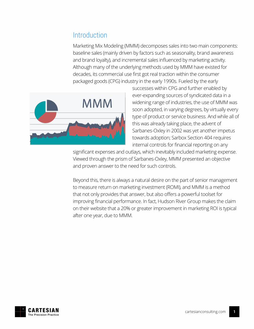
IntroductionMarketing Mix Modeling (MMM) decomposes sales into two main components: baseline sales (mainly driven by factors such as seasonality, brand awareness and brand loyalty), and incremental sales influenced by marketing activity. Although many of the underlying methods used by MMM have existed for decades, its commercial use first got real traction within the consumer packaged goods (CPG) industry in the early 1990s. Fueled by the early

successes within CPG and further enabled by ever-expanding sources of syndicated data in a widening range of industries, the use of MMM was soon adopted, in varying degrees, by virtually every type of product or service business. And while all of this was already taking place, the advent of Sarbanes-Oxley in 2002 was yet another impetus towards adoption; Sarbox Section 404 requires internal controls for financial reporting on any

significant expenses and outlays, which inevitably included marketing expense. Viewed through the prism of Sarbanes-Oxley, MMM presented an objective and proven answer to the need for such controls.

Beyond this, there is always a natural desire on the part of senior management to measure return on marketing investment (ROMI), and MMM is a method that not only provides that answer, but also offers a powerful toolset for improving financial performance. In fact, Hudson River Group makes the claim on their website that a 20% or greater improvement in marketing ROI is typical after one year, due to MMM.


BUILDING BLOCKS AND SCOPE

Dependent VariablesDetermine what dependent variable the MMM project will measure. Usually this will be sales or profit, but it in some cases it could also be a customer metric such as traffic, acquisitions, app downloads, or even brand response such as awareness or consideration.

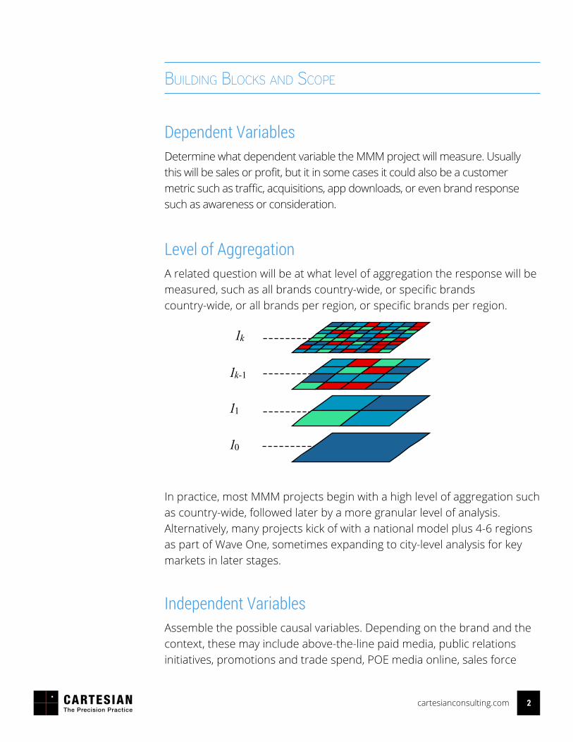
Level of AggregationA related question will be at what level of aggregation the response will be measured, such as all brands country-wide, or specific brands country-wide, or all brands per region, or specific brands per region.

In practice, most MMM projects begin with a high level of aggregation such as country-wide, followed later by a more granular level of analysis. Alternatively, many projects kick of with a national model plus 4-6 regions as part of Wave One, sometimes expanding to city-level analysis for key markets in later stages.

Independent VariablesAssemble the possible causal variables. Depending on the brand and the context, these may include above-the-line paid media, public relations initiatives, promotions and trade spend, POE media online, sales force

1k

1k-1

11

10


activity, and various social media metrics. Other explanatory variables are possible, including for example, number and distribution of stores or branches, and seasonality indicators.

Unit of Measure, Unit of TimeFor each independent variable, a unit of measure per unit of time is needed. Daily sales data generally has too much variation, leading to lower precision. Often the unit of time is a week. For the independent variables, the unit of measure might be dollars spent per week, and for the dependent variable, the unit might be sales per week. Another frequently-used causal measure is gross rating points (GRPs) per week, which reflects the percent of the target market reached, multiplied by the exposure frequency. For example, if a brand were to advertise to 20% of the target market and give them 5 exposures, they would have achieved 120 GRPs. In some cases, the working definition of GRP is simplified to just the sum of total rating points (TRPs) in a media schedule.

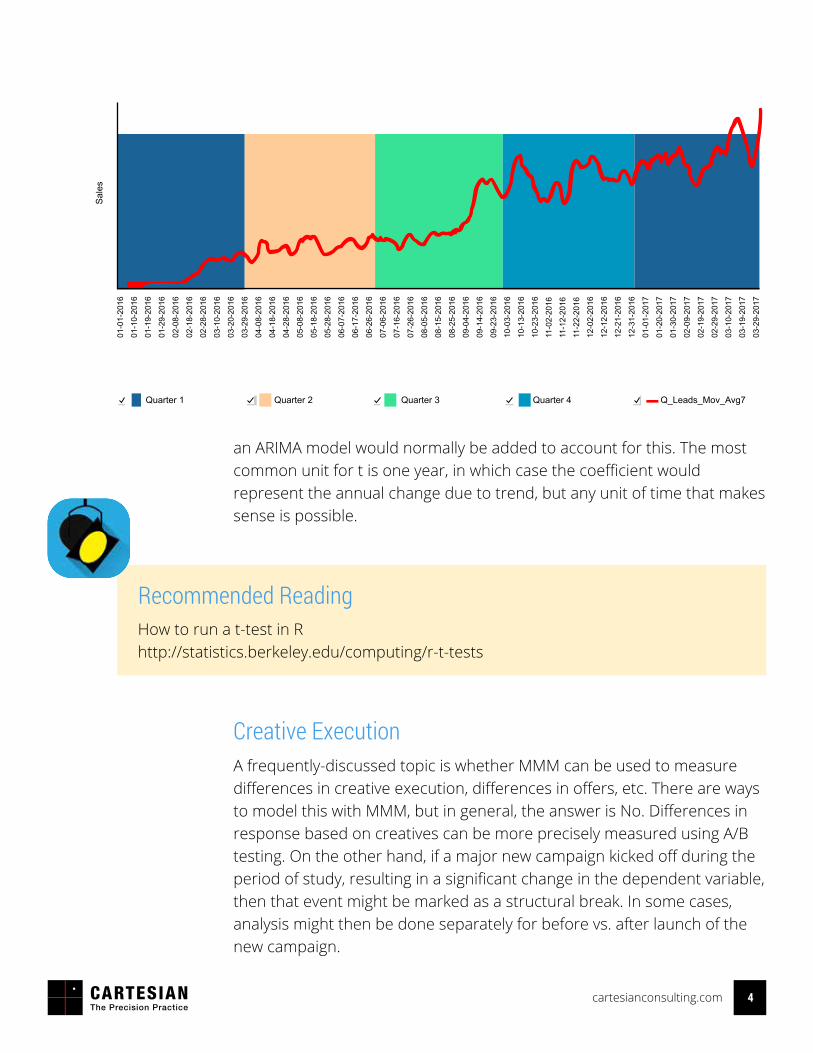
SeasonalityMost companies have seasonality in their business, so seasonality is another independent variable that generally is included in the model. For example, to capture month of the year, one might create 11 dummy variables, each coded as 0 or 1.

TrendA standard t-test can be used to indicate whether or not there is a significant trend in the data, or if the hypothesis is that there is a trend in one particular direction, then a one-tailed t-test can be used. Either way, if the data suggest that there is a trend, then a dummy variable (t or t2) or


an ARIMA model would normally be added to account for this. The most common unit for t is one year, in which case the coefficient would represent the annual change due to trend, but any unit of time that makes sense is possible.

Creative ExecutionA frequently-discussed topic is whether MMM can be used to measure differences in creative execution, differences in offers, etc. There are ways to model this with MMM, but in general, the answer is No. Differences in response based on creatives can be more precisely measured using A/B testing. On the other hand, if a major new campaign kicked off during the period of study, resulting in a significant change in the dependent variable, then that event might be marked as a structural break. In some cases, analysis might then be done separately for before vs. after launch of the new campaign.

01-0

1-20

16

01-1

0-20

16

01-1

9-20

16

01-2

9-20

16

02-0

8-20

16

02-1

8-20

16

02-2

8-20

16

03-1

0-20

16

03-2

0-20

16

03-2

9-20

16

04-0

8-20

16

04-1

8-20

16

04-2

8-20

16

05-0

8-20

16

05-1

8-20

16

05-2

8-20

16

06-0

7-20

16

06-1

7-20

16

06-2

6-20

16

07-0

6-20

16

07-1

6-20

16

07-2

6-20

16

08-0

5-20

16

08-1

5-20

16

08-2

5-20

16

09-0

4-20

16

09-1

4-20

16

09-2

3-20

16

10-0

3-20

16

10-1

3-20

16

10-2

3-20

16

11-0

2-20

16

11-1

2-20

16

11-2

2-20

16

12-0

2-20

16

12-1

2-20

16

12-2

1-20

16

12-3

1-20

16

01-0

1-20

17

01-2

0-20

17

01-3

0-20

17

02-0

9-20

17

02-1

9-20

17

02-2

9-20

17

03-1

0-20

17

03-1

9-20

17

03-2

9-20

17

Quarter 1 Quarter 2 Quarter 3 Quarter 4

Sal

es

Q_Leads_Mov_Avg7

How to run a t-test in Rhttp://statistics.berkeley.edu/computing/r-t-tests

Recommended Reading


DATA PREPARATION AND TRANSFORMATION

At least two years of data (104 weeks) for both the independent and dependent variables is desirable. Data that is not available in a weekly form generally needs to be transformed into such a form. For example, billboard advertising may be paid quarterly, but the spend can be subdivided as an amount invested per week.

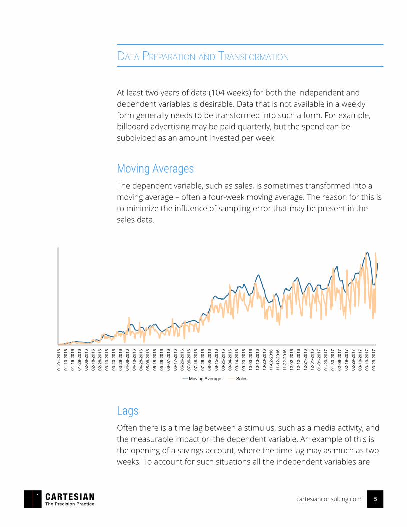
Moving AveragesThe dependent variable, such as sales, is sometimes transformed into a moving average – often a four-week moving average. The reason for this is to minimize the influence of sampling error that may be present in the sales data.

LagsOften there is a time lag between a stimulus, such as a media activity, and the measurable impact on the dependent variable. An example of this is the opening of a savings account, where the time lag may as much as two weeks. To account for such situations all the independent variables are

01-0

1-2

016

01-1

0-2

016

01-1

9-2

016

01-2

9-2

016

02-0

8-2

016

02-1

8-2

016

02-2

8-2

016

03-1

0-2

016

03-2

0-2

016

03-2

9-2

016

04-0

8-2

016

04-1

8-2

016

04-2

8-2

016

05-0

8-2

016

05-1

8-2

016

05-2

8-2

016

06-0

7-2

016

06-1

7-2

016

06-2

6-2

016

07-0

6-2

016

07-1

6-2

016

07-2

6-2

016

08-0

5-2

016

08-1

5-2

016

08-2

5-2

016

09-0

4-2

016

09-1

4-2

016

09-2

3-2

016

10-0

3-2

016

10-1

3-2

016

10-2

3-2

016

11-0

2-2

016

11-1

2-2

016

11-2

2-2

016

12-0

2-2

016

12-1

2-2

016

12-2

1-2

016

12-3

1-2

016

01-0

1-2

017

01-2

0-2

017

01-3

0-2

017

02-0

9-2

017

02-1

9-2

017

02-2

9-2

017

03-1

0-2

017

03-1

9-2

017

03-2

9-2

017

Moving Average Sales


lagged by the appropriate number of periods, as determined through business inputs and correlation study.

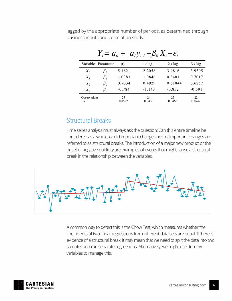
Structural BreaksTime series analysis must always ask the question: Can this entire timeline be considered as a whole, or did important changes occur? Important changes are referred to as structural breaks. The introduction of a major new product or the onset of negative publicity are examples of events that might cause a structural break in the relationship between the variables.

A common way to detect this is the Chow Test, which measures whether the coefficients of two linear regressions from different data sets are equal. If there is evidence of a structural break, it may mean that we need to split the data into two samples and run separate regressions. Alternatively, we might use dummy variables to manage this.

Y = a + a y +ß X +εVariable Parameter (t) 1- t lag 2-t lag 3-t lag

ObservationsR2

250.8522

240.8433

230.8463

220.8747

X0

X1

X2

X3

β0

β1

β2

β3

5.16211.03830.7034-0.784

2.20581.08460.4929-1.143

3.98160.84810.61844-0.852

3.93950.70170.6257-0.591

t 0 1 t-1 0 t t


BUILDING THE MMM MODEL

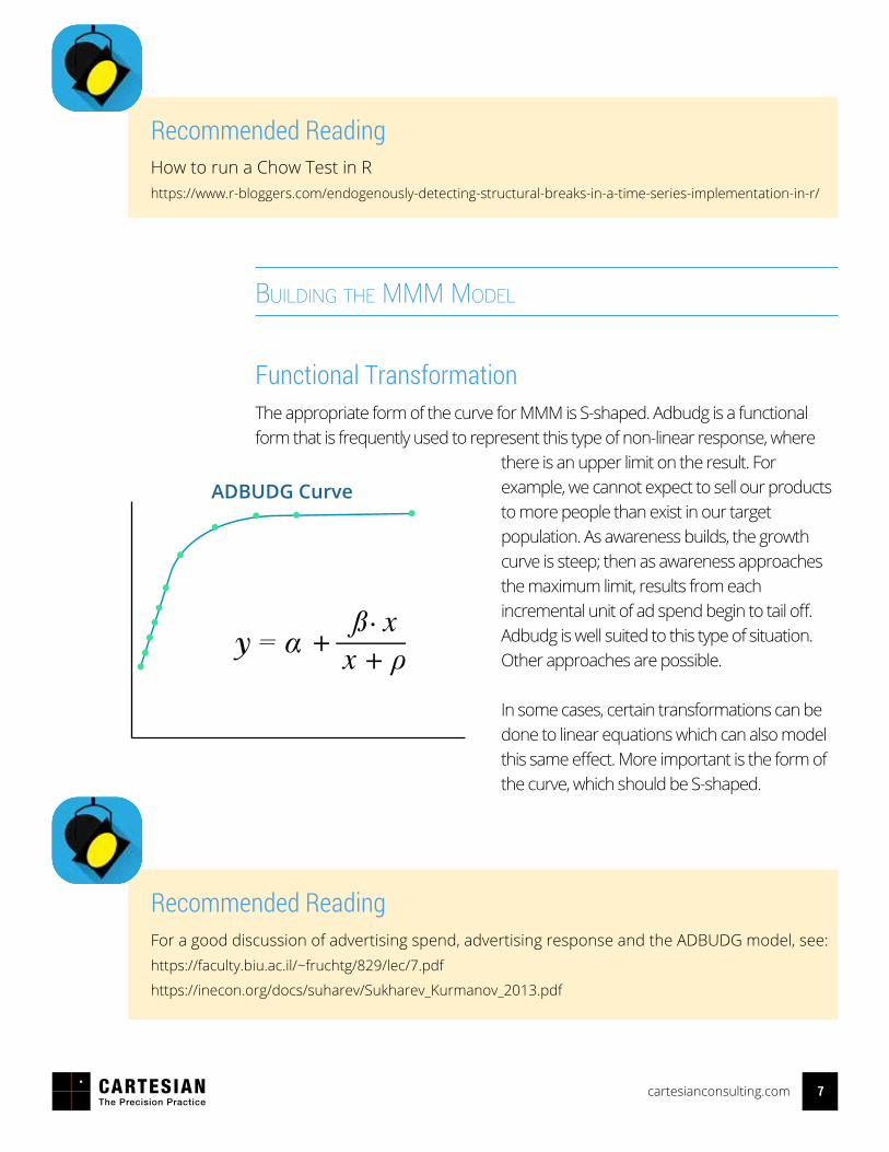
Functional TransformationThe appropriate form of the curve for MMM is S-shaped. Adbudg is a functional form that is frequently used to represent this type of non-linear response, where

there is an upper limit on the result. For example, we cannot expect to sell our products to more people than exist in our target population. As awareness builds, the growth curve is steep; then as awareness approaches the maximum limit, results from each incremental unit of ad spend begin to tail off. Adbudg is well suited to this type of situation. Other approaches are possible.

In some cases, certain transformations can be done to linear equations which can also model this same effect. More important is the form of the curve, which should be S-shaped.

For a good discussion of advertising spend, advertising response and the ADBUDG model, see:https://faculty.biu.ac.il/~fruchtg/829/lec/7.pdf

https://inecon.org/docs/suharev/Sukharev_Kurmanov_2013.pdf

Recommended Reading

How to run a Chow Test in Rhttps://www.r-bloggers.com/endogenously-detecting-structural-breaks-in-a-time-series-implementation-in-r/

Recommended Reading

ADBUDG Curve

ß. xx + ρ+α


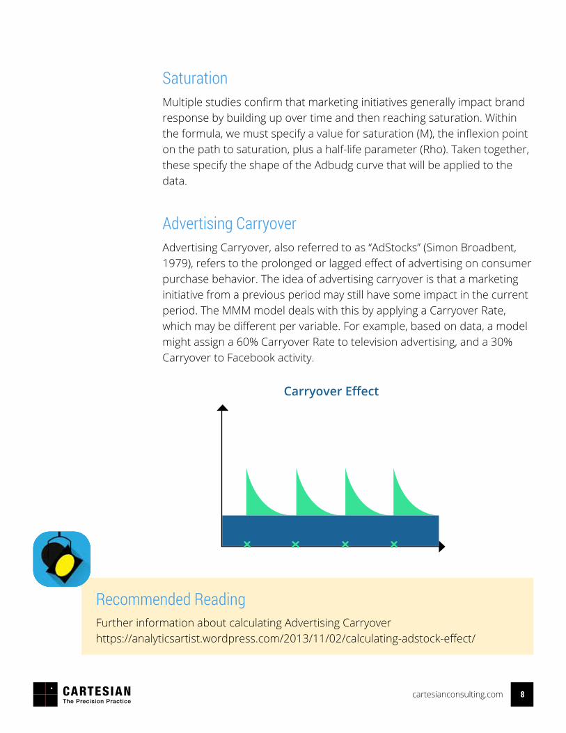
SaturationMultiple studies confirm that marketing initiatives generally impact brand response by building up over time and then reaching saturation. Within the formula, we must specify a value for saturation (M), the inflexion point on the path to saturation, plus a half-life parameter (Rho). Taken together, these specify the shape of the Adbudg curve that will be applied to the data.

Advertising CarryoverAdvertising Carryover, also referred to as “AdStocks” (Simon Broadbent, 1979), refers to the prolonged or lagged effect of advertising on consumer purchase behavior. The idea of advertising carryover is that a marketing initiative from a previous period may still have some impact in the current period. The MMM model deals with this by applying a Carryover Rate, which may be different per variable. For example, based on data, a model might assign a 60% Carryover Rate to television advertising, and a 30% Carryover to Facebook activity.

Carryover Effect

Further information about calculating Advertising Carryoverhttps://analyticsartist.wordpress.com/2013/11/02/calculating-adstock-effect/

Recommended Reading


VALIDATION

Once an initial model is built, it is checked in various ways. Some of the statistics and methods that are used for this purpose include R2, MAPE, F Tests, residual plots, VIF and machine learning.

R2

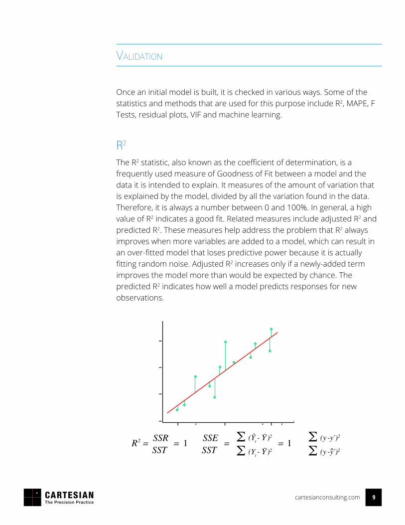
The R2 statistic, also known as the coefficient of determination, is a frequently used measure of Goodness of Fit between a model and the data it is intended to explain. It measures of the amount of variation that is explained by the model, divided by all the variation found in the data. Therefore, it is always a number between 0 and 100%. In general, a high value of R2 indicates a good fit. Related measures include adjusted R2 and predicted R2. These measures help address the problem that R2 always improves when more variables are added to a model, which can result in an over-fitted model that loses predictive power because it is actually fitting random noise. Adjusted R2 increases only if a newly-added term improves the model more than would be expected by chance. The predicted R2 indicates how well a model predicts responses for new observations.

R 1 1= = = =SSRSST

2 SSE (Ŷt - Ῡ)2

SSTΣ

(Yt - Ῡ)2ΣΣΣ


MAPEBesides predicted R2, another common measure of forecast accuracy is Mean Absolute Deviation (MAD), also called Mean Absolute Error (MAE). This is the average of the absolute deviation (error) between the values predicted by a model vs. the actual values. Mean Absolute Percentage Error (MAPE) builds upon this. It is a measure the absolute prediction error as a percentage of the actual values in the data.

F Test of Overall SignificanceThis is another frequently-used measure of Goodness of Fit of a model. It answers whether the relationship between the predictor variables and the dependent variable is statistically significant. Unlike t-tests that can assess only one regression coefficient at a time, the F-test can assess multiple coefficients simultaneously.

For a good introduction to evaluating model performance, see:https://www.otexts.org/fpp/4/4

Recommended Reading


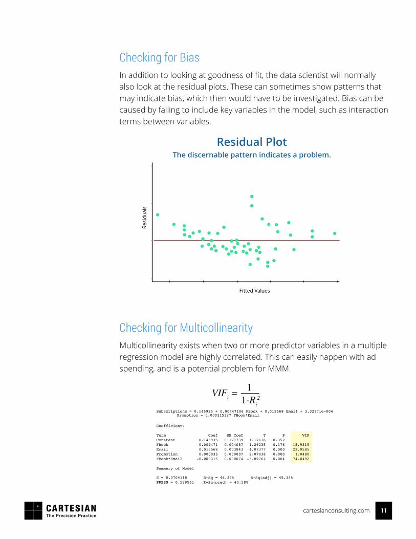
Checking for BiasIn addition to looking at goodness of fit, the data scientist will normally also look at the residual plots. These can sometimes show patterns that may indicate bias, which then would have to be investigated. Bias can be caused by failing to include key variables in the model, such as interaction terms between variables.

Checking for MulticollinearityMulticollinearity exists when two or more predictor variables in a multiple regression model are highly correlated. This can easily happen with ad spending, and is a potential problem for MMM.

Fitted Values

Resi

dual

sResidual Plot

The discernable pattern indicates a problem.

VIFi = 11-Ri

2

Subscriptions = 0.145925 + 0.00447106 FBook + 0.015568 Email + 3.32771e-004

Coefficients

Summary of Model

S = 0.0704118 R-Sq = 46.32% R-Sq(adj) = 45.33%PRESS = 0.589561 R-Sq(pred) = 40.58%

TermConstantFBookEmailPromotion FBook*Email

Coef0.1459350.0044710.0155680.000033-0.000315

SE Coef0.1217390.0040870.0038430.0000070.000074

T1.176161.262354.073772.07436-3.89762

P0.3520.1760.0000.0000.004

VIF

15.931522.95851.048074.0492

Promotion - 0.000315327 FBook*Email


The issue with multicollinearity is that it can result in unstable estimates that make it difficult to assess which of the individual types of media had how much effect on the dependent variable, such as sales.

Variance-inflation factor (VIF) is used to measures this. A VIF of ≥ 10 implies that the independent variables are 90% correlated, which means that there is a problem with multicollinearity in the data. In such a case, the model will usually need to be adjusted to account for this.

Model EvaluationTo evaluate the MMM model, the data scientist typically holds out a sample of data, and uses the proposed model to predict results from the holdout sample. Sometimes an additional holdout sample is reserved for a final validation test. The purpose of this is to avoid over-fitting the MMM model to the specific training data, thus failing to properly generalize the results. Trade-offs exist in this process. If too much data is held out for validation testing, then less data will be available for the initial model build. A hybrid approach, known as cross-validation, also exists to help manage these trade-offs.

How to calculate VIF in Rhttps://beckmw.wordpress.com/2013/02/05/collinearity-and-stepwise-vif-selection/

Recommended Reading


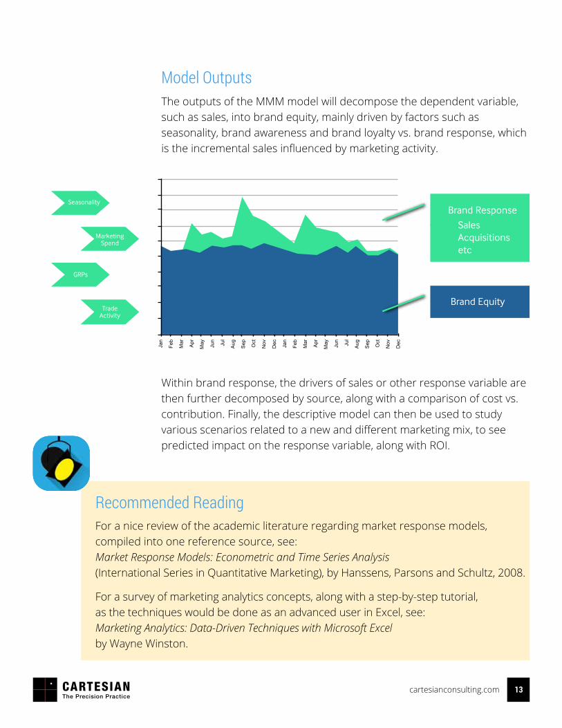
Model OutputsThe outputs of the MMM model will decompose the dependent variable, such as sales, into brand equity, mainly driven by factors such as seasonality, brand awareness and brand loyalty vs. brand response, which is the incremental sales influenced by marketing activity.

Within brand response, the drivers of sales or other response variable are then further decomposed by source, along with a comparison of cost vs. contribution. Finally, the descriptive model can then be used to study various scenarios related to a new and different marketing mix, to see predicted impact on the response variable, along with ROI.

Jan

Feb

Mar

Apr

May Jun

Jul

Aug

Sep Oct

Nov

Dec Jan

Feb

Mar

Apr

May Jun

Jul

Aug

Sep Oct

Nov

Dec

SalesAcquisitionsetc

Brand Response

Brand Equity

Seasonality

GRPs

MarketingSpend

TradeActivity

For a nice review of the academic literature regarding market response models, compiled into one reference source, see:Market Response Models: Econometric and Time Series Analysis (International Series in Quantitative Marketing), by Hanssens, Parsons and Schultz, 2008.

For a survey of marketing analytics concepts, along with a step-by-step tutorial, as the techniques would be done as an advanced user in Excel, see:Marketing Analytics: Data-Driven Techniques with Microsoft Excelby Wayne Winston.

Recommended Reading


SELECTING AND USING THE MODEL

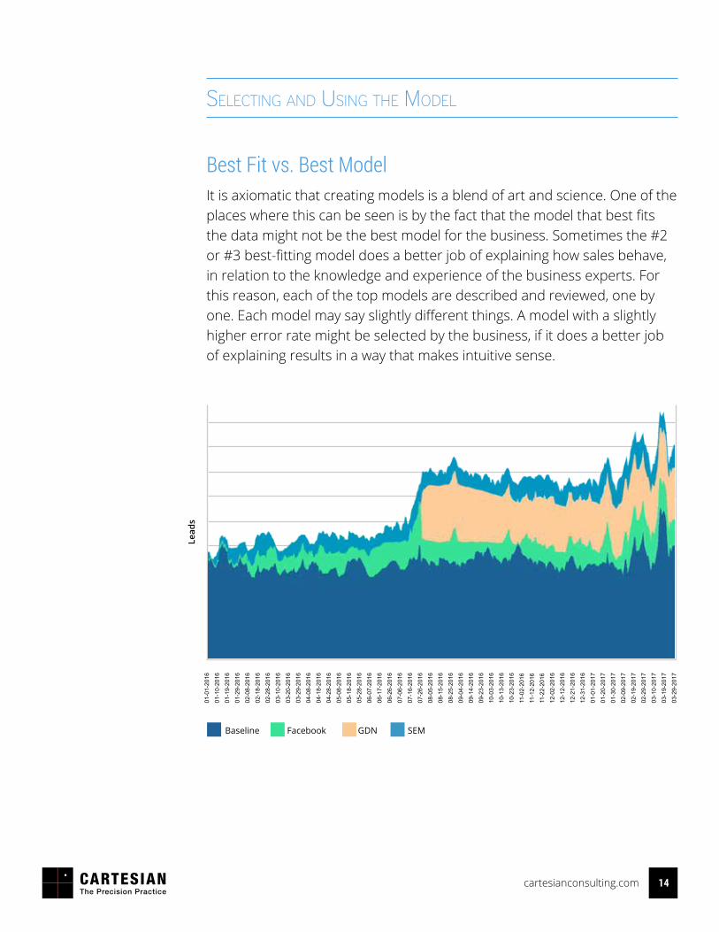
Best Fit vs. Best ModelIt is axiomatic that creating models is a blend of art and science. One of the places where this can be seen is by the fact that the model that best fits the data might not be the best model for the business. Sometimes the #2 or #3 best-fitting model does a better job of explaining how sales behave, in relation to the knowledge and experience of the business experts. For this reason, each of the top models are described and reviewed, one by one. Each model may say slightly different things. A model with a slightly higher error rate might be selected by the business, if it does a better job of explaining results in a way that makes intuitive sense.

Lead

s01

-01-

2016

01-1

0-20

16

01-1

9-20

16

01-2

9-20

16

02-0

8-20

16

02-1

8-20

16

02-2

8-20

16

03-1

0-20

16

03-2

0-20

16

03-2

9-20

16

04-0

8-20

16

04-1

8-20

16

04-2

8-20

16

05-0

8-20

16

05-1

8-20

16

05-2

8-20

16

06-0

7-20

16

06-1

7-20

16

06-2

6-20

16

07-0

6-20

16

07-1

6-20

16

07-2

6-20

16

08-0

5-20

16

08-1

5-20

16

08-2

5-20

16

09-0

4-20

16

09-1

4-20

16

09-2

3-20

16

10-0

3-20

16

10-1

3-20

16

10-2

3-20

16

11-0

2-20

16

11-1

2-20

16

11-2

2-20

16

12-0

2-20

16

12-1

2-20

16

12-2

1-20

16

12-3

1-20

16

01-0

1-20

17

01-2

0-20

17

01-3

0-20

17

02-0

9-20

17

02-1

9-20

17

02-2

9-20

17

03-1

0-20

17

03-1

9-20

17

03-2

9-20

17

Baseline Facebook GDN SEM


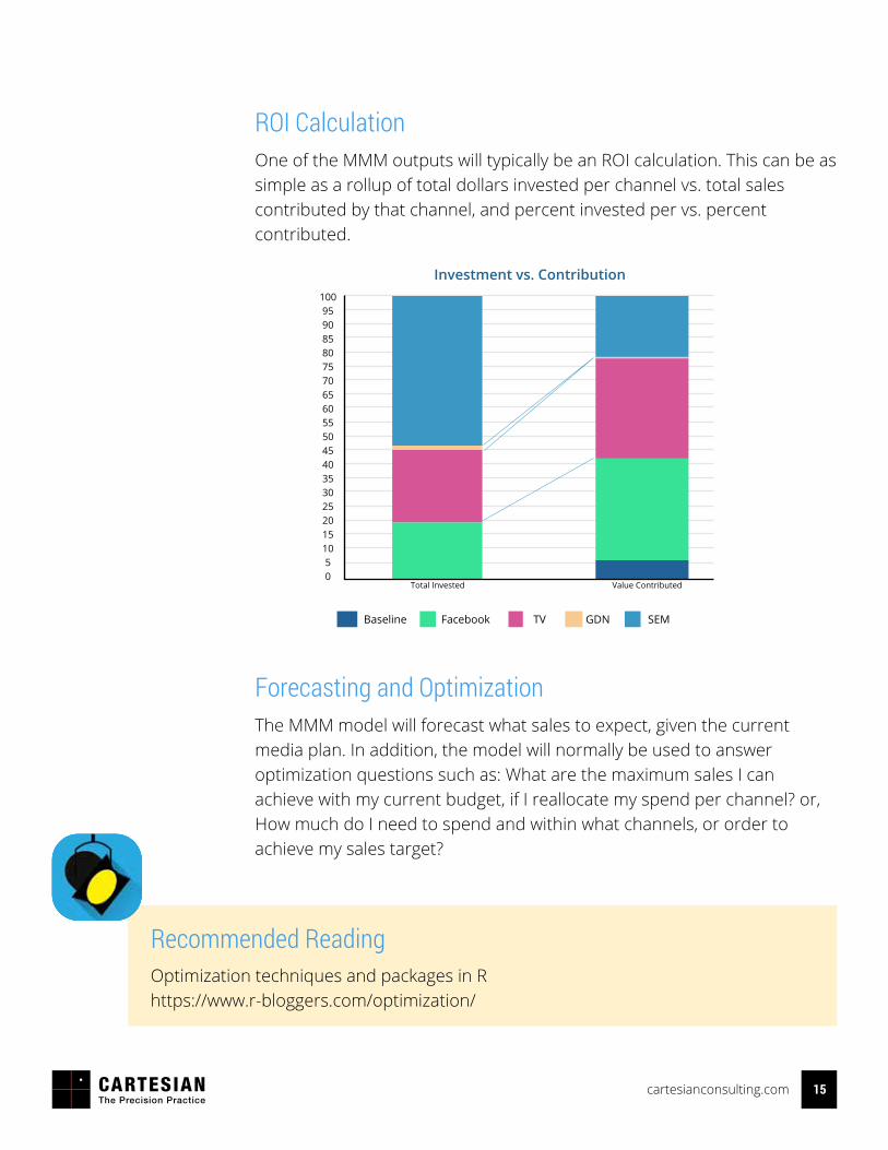
ROI CalculationOne of the MMM outputs will typically be an ROI calculation. This can be as simple as a rollup of total dollars invested per channel vs. total sales contributed by that channel, and percent invested per vs. percent contributed.

Forecasting and OptimizationThe MMM model will forecast what sales to expect, given the current media plan. In addition, the model will normally be used to answer optimization questions such as: What are the maximum sales I can achieve with my current budget, if I reallocate my spend per channel? or, How much do I need to spend and within what channels, or order to achieve my sales target?

Investment vs. Contribution10095908580757065605550454035302520151050

Total Invested Value Contributed

Baseline Facebook GDN SEMTV

Optimization techniques and packages in Rhttps://www.r-bloggers.com/optimization/

Recommended Reading


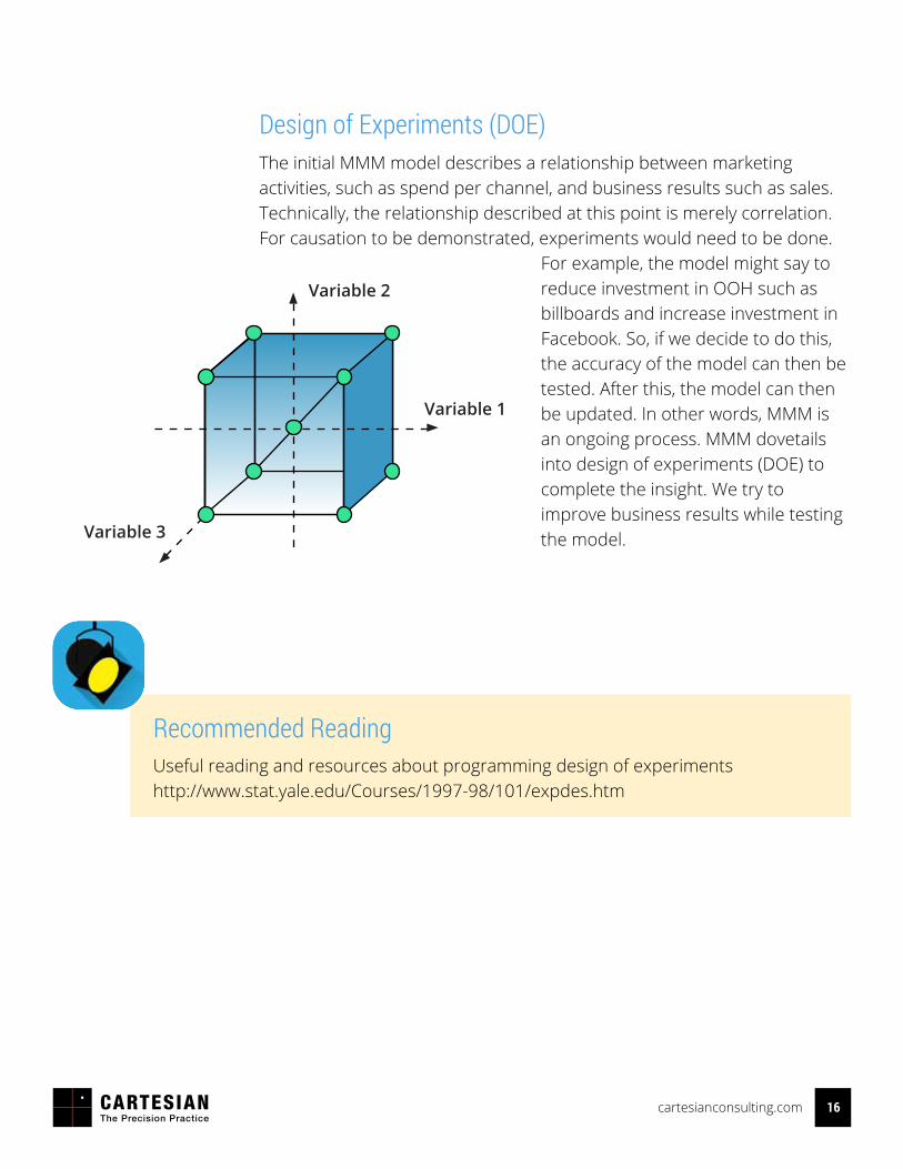
Design of Experiments (DOE)The initial MMM model describes a relationship between marketing activities, such as spend per channel, and business results such as sales. Technically, the relationship described at this point is merely correlation. For causation to be demonstrated, experiments would need to be done.

For example, the model might say to reduce investment in OOH such as billboards and increase investment in Facebook. So, if we decide to do this, the accuracy of the model can then be tested. After this, the model can then be updated. In other words, MMM is an ongoing process. MMM dovetails into design of experiments (DOE) to complete the insight. We try to improve business results while testing the model.

Variable 2

Variable 1

Variable 3

Useful reading and resources about programming design of experimentshttp://www.stat.yale.edu/Courses/1997-98/101/expdes.htm

Recommended Reading


LIMITATIONS AND CAVEATS

Like any tool, MMM should be used for the purpose it was created.

For example, one of the limitations of MMM is a bias against activities that build brand equity. This is a logical result of the fact that brand equity is reflected in the MMM baseline as an “unexplained response.” The truth is, this unexplained response was probably the result of many years of investments, including investments in brand building. MMM helps marketing leaders to maximize marketing efficiency (sales volume divided by cost), which is usually a short-term metric. Longer-term effects of marketing are reflected in brand equity and are usually not captured by MMM. What this means is the marketing leadership must still use common sense to balance investments across short-term and longer-term objectives. Alternatively, traditional MMM can be combined with longer-term brand-equity models, in order to get a more complete and balanced perspective on where to invest.

Another limitation of MMM stems from different levels of precision across media types. For example, exposure to television ads can be measured with a great deal of precision, whereas there is less precision in regard to exposure to magazine advertising. Consequently, MMM models are usually biased in favor of TV vs. magazines, due to the better precision for television, so this is something that needs to be considered when taking action based on such models.

In addition, some marketing initiatives may actually be quite effective in targeting specific demographics or other groups, but their impact might be lost when rolled up with aggregate data at the national or even at a regional level, so other evidence may be needed to supplement MMM in regard to certain types of highly-targeted campaigns.

Finally, MMM is best suited for use in cases where historical data is available, and is not as useful for evaluation of marketing investments in new products. Not only does relatively short history make marketing-mix results unstable, but also product launch generally involves a


higher-than-typical investment in brand building. This means that measures such as awareness and consideration are more important and useful at this stage than they would be for a mature product. Used too early during a product launch, traditional MMM would probably signal a need for more promotional activity, which might actually damage the long-term equity of the brand being launched.

About the Authors

Jim GriffinAmericas Director


Tapan KhopkarHead of Advanced Analytics


Jim Griffin has twenty years of analytics, CRM, and loyalty experience in multiple markets, including USA, Latin America and Asia. He holds an MBA from the University of Minnesota where he graduated with a 4.0 GPA. He did post-graduate study in statistics while living in Asia Pacific, and is Six Sigma Black Belt trained. Jim is also a faculty member with the International Institute of Digital Marketing (IIDM).

A PhD in Information from the University of Michigan, Tapan Khopkar joined Cartesian in 2008 and, since that time, has led some of the company’s most challenging and complex analytics assignments. He has extensive knowledge of statistical modelling, machine learning and AI and has been instrumental in developing Cartesian’s analytical frameworks and techniques. Tapan leads the Advanced Analytics practice, and the Marketing Mix Modelling efforts. He has several publications in international journals, and regularly participates in research and industry conferences.


Cartesian Consulting is a data analytics firm, specialized in customer and marketing analytics. We provide highly-customized analytics services to 70 clients worldwide. Our work includes attribution and marketing mix optimization, customer segmentation, customer lifetime value models, predictive models, cross-sell / up-sell models, market basket analysis, pricing and promo optimization, as well as analytics of web and digital data. In particular, our MMM models have been used by publishers such as Facebook.

The team consists of 150 people, highly skilled at statistics and machine learning. Tools and methods used in various projects have included regression, clustering, random forest, boosting, Markov chains, genetic algorithms, Pareto NBD, SVM, collaborative filtering, time series forecasting and linear programming. Cartesian was named the Boutique Analytics firm of the Year at Cypher 2016.

Contact UsIndiaShikha Lath: [email protected]

AmericasJim Griffin: [email protected]

ASEANDeepa Ghosh: [email protected]

the mmm playbook - cartesian consulting · the mmm playbook. cartesianconsulting.com 1 introduction...

Documents