the mm, me, ml, el, ef and gmm approaches to estimation… · journal of econometrics 107 (2002)...
TRANSCRIPT

Journal of Econometrics 107 (2002) 51–86www.elsevier.com/locate/econbase
The MM, ME, ML, EL, EF and GMMapproaches to estimation: a synthesis
Anil K. Beraa ;∗, Yannis Biliasb
aDepartment of Economics, University of Illinois, 1206 S. 6th Street, Champaign, IL 61820, USAbDepartment of Economics, University of Cyprus, P.O. Box 20537, 1678 Nicosia, Cyprus
Abstract
The 20th century began on an auspicious statistical note with the publication of Karl Pearson’s(Philos. Mag. Ser. 50 (1900) 157) goodness-of-4t test, which is regarded as one of the mostimportant scienti4c breakthroughs. The basic motivation behind this test was to see whether anassumed probability model adequately described the data at hand. Pearson (Philos. Trans. Roy.Soc. London Ser. A 185 (1894) 71) also introduced a formal approach to statistical estimationthrough his method of moments (MM) estimation. Ronald A. Fisher, while he was a third yearundergraduate at the Gonville and Caius College, Cambridge, suggested the maximum likeli-hood estimation (MLE) procedure as an alternative to Pearson’s MM approach. In 1922 Fisherpublished a monumental paper that introduced such basic concepts as consistency, e<ciency,su<ciency—and even the term “parameter” with its present meaning. Fisher (Philos. Trans. Roy.Soc. London Ser. A 222 (1922) 309) provided the analytical foundation of MLE and studied itse<ciency relative to the MM estimator. Fisher (J. Roy. Statist. Soc. 87 (1924a) 442) establishedthe asymptotic equivalence of minimum �2 and ML estimators and wrote in favor of usingminimum �2 method rather than Pearson’s MM approach. Recently, econometricians have foundworking under assumed likelihood functions restrictive, and have suggested using a generalizedversion of Pearson’s MM approach, commonly known as the GMM estimation procedure asadvocated in Hansen (Econometrica 50 (1982) 1029). Earlier, Godambe (Ann. Math. Statist. 31(1960) 1208) and Durbin (J. Roy. Statist. Soc. Ser. B 22 (1960) 139) developed the estimatingfunction (EF) approach to estimation that has been proven very useful for many statistical models.A fundamental result is that score is the optimum EF. Ferguson (Ann. Math. Statist. 29 (1958)1046) considered an approach very similar to GMM and showed that estimation based on thePearson �2 statistic is equivalent to e<cient GMM. Golan et al. (Maximum Entropy Economet-rics: Robust Estimation with Limited Data. Wiley, New York, 1996) developed entropy-basedformulation that allowed them to solve a wide range of estimation and inference problems ineconometrics. More recently, Imbens et al. (Econometrica 66 (1998) 333), Kitamura and Stutzer(Econometrica 65 (1997) 861) and Mittelhammer et al. (Econometric Foundations. CambridgeUniversity Press, Cambridge, 2000) put GMM within the framework of empirical likelihood
∗Corresponding author. Tel.: +1-217-333-4596; fax: +1-217-244-6678.E-mail address: [email protected] (A.K. Bera).
0304-4076/02/$ - see front matter c© 2002 Elsevier Science B.V. All rights reserved.PII: S 0304 -4076(01)00113 -0

52 A.K. Bera, Y. Bilias / Journal of Econometrics 107 (2002) 51–86
(EL) and maximum entropy (ME) estimation. It can be shown that many of these estimationtechniques can be obtained as special cases of minimizing Cressie and Read (J. Roy. Statist. Soc.Ser. B 46 (1984) 440) power divergence criterion that comes directly from the Pearson (1900)�2 statistic. In this way we are able to assimilate a number of seemingly unrelated estimationtechniques into a uni4ed framework. c© 2002 Elsevier Science B.V. All rights reserved.
JEL classi4cation: C13; C52
Keywords: Karl Pearson’s goodness-of-4t statistic; Entropy; Method of moment; Estimating function;Likelihood; Empirical likelihood; Generalized method of moments; Power divergence criterion; History ofestimation
1. Prologue: Karl Pearson’s method of moment estimation and �2 test, and entropy
In this paper we are going to discuss various methods of estimation, especially thosedeveloped in the 20th century, beginning with a review of some developments in statis-tics at the close of the 19th century. In 1892 W.F. Raphael Weldon, a zoologist turnedstatistician, requested Karl Pearson (1857–1936) to analyze a set of data on crabs. Aftersome investigation Pearson realized that he could not 4t the usual normal distributionto this data. By the early 1890s Pearson had developed a class of distributions thatlater came to be known as the Pearson system of curves, which is much broader thanthe normal distribution. However, for the crab data Pearson’s own system of curveswas not good enough. He dissected this “abnormal frequency curve” into two normalcurves as follows:
f(y) = �f1(y) + (1− �)f2(y); (1)
where
fj(y) =1√2��j
exp
[− 12�2j
(y − j)2]; j = 1; 2:
This model has 4ve parameters 1 (�; 1; �21 ; 2; �22). Previously, there had been no
method available to estimate such a model. Pearson quite unceremoniously suggesteda method that simply equated the 4rst 4ve population moments to the respective sam-ple counterparts. It was not easy to solve 4ve highly nonlinear equations. Therefore,Pearson took an analytical approach of eliminating one parameter in each step. Af-ter considerable algebra he found a ninth-degree polynomial equation in one unknown.Then, after solving this equation and by repeated back-substitutions, he found solutionsto the 4ve parameters in terms of the 4rst 4ve sample moments. It was around theautumn of 1893 he completed this work and it appeared in 1894. And this was thebeginning of the method of moment (MM) estimation. There is no general theory in
1 The term “parameter” was introduced by Fisher (1922, p. 311) [also see footnote 16]. Karl Pearson de-scribed the “parameters” as “constants” of the “curve”. Fisher (1912) also used “frequency curve”. However,in Fisher (1922) he used the term “distribution” throughout. “Probability density function” came much later,in Wilks (1943, p. 8) (see, David, 1995).
A.K. Bera, Y. Bilias / Journal of Econometrics 107 (2002) 51–86 53
Pearson (1894). The paper is basically a worked-out “example” (though a very di<cultone as the 4rst illustration of MM estimation) of a new estimation method. 2
After an experience of “some eight years” in applying the MM to a vast range ofphysical and social data, Pearson (1902) provided some “theoretical” justi4cation ofhis methodology. Suppose we want to estimate the parameter vector �=(�1; �2; : : : ; �p)′
of the probability density function f(y; �). By a Taylor series expansion of f(y) ≡f(y; �) around y = 0, we can write
f(y) = 0 + 1y + 2y2
2!+ 3
y3
3!+ · · ·+ p
yp
p!+ R; (2)
where 0; 1; 2; : : : ; p depends on �1; �2; : : : ; �p and R is the remainder term. LetQf(y) be the ordinate corresponding to y given by observations. Therefore, the prob-lem is to 4t a smooth curve f(y; �) to p histogram ordinates given by Qf(y). Thenf(y) − Qf(y) denotes the distance between the theoretical and observed curve at thepoint corresponding to y, and our objective would be to make this distance as smallas possible by a proper choice of 0; 1; 2; : : : ; p (see Pearson, 1902, p. 268). 3 Al-though Pearson discussed the 4t of f(y) to p histogram ordinates Qf(y), he proceededto 4nd a “theoretical” version of f(y) that minimizes (see Mensch, 1980)∫
[f(y)− Qf(y)]2 dy: (3)
Since f(:) is the variable, the resulting equation is∫[f(y)− Qf(y)]�f dy = 0; (4)
where, from (2), the diRerential �f can be written as
�f =p∑j=0
(� j
yj
j!+
@R@ j
� j
): (5)
Therefore, we can write Eq. (4) as∫[f(y)− Qf(y)]
p∑j=0
(� j
yj
j!+
@R@ j
� j
)dy
=p∑j=0
∫[f(y)− Qf(y)]
(yj
j!+
@R@ j
)dy� j = 0: (6)
2 Shortly after Karl Pearson’s death, his son Egon Pearson provided an account of life and work ofthe elder Pearson (see Pearson, 1936a). He summarized (pp. 219–220) the contribution of Pearson (1894)stating, “The paper is particularly noteworthy for its introduction of the method of moments as a means of4tting a theoretical curve to observed data. This method is not claimed to be the best but is advocated fromthe utilitarian standpoint on the grounds that it appears to give excellent 4ts and provides algebraic solutionsfor calculating the constants of the curve which are analytically possible”.
3 It is hard to trace the 4rst use of smooth non-parametric density estimation in the statistics literature.Koenker (2000, p. 349) mentioned Galton’s (1885) illustration of “regression to the mean” where Galtonaveraged the counts from the four adjacent squares to achieve smoothness. Karl Pearson’s minimization ofthe distance between f(y) and Qf(y) looks remarkably modern in terms of ideas and could be viewed as amodern-equivalent of smooth non-parametric density estimation (see also Mensch, 1980).

54 A.K. Bera, Y. Bilias / Journal of Econometrics 107 (2002) 51–86
Since the quantities 0; 1; 2; : : : ; p are at our choice, for (6) to hold, each componentshould be independently zero, i.e., we should have∫
[f(y)− Qf(y)](yj
j!+
@R@ j
)dy = 0; j = 0; 1; 2; : : : ; p; (7)
which is same as
j = mj − j!∫
[f(y)− Qf(y)](@R@ j
)dy; j = 0; 1; 2; : : : ; p: (8)
Here j and mj are, respectively, the jth moment corresponding to the theoretical curvef(y) and the observed curve Qf(y). 4 Pearson (1902) then ignored the integral termsarguing that they involve the small factor f(y) − Qf(y), and the remainder term R,which by “hypothesis” is small for large enough sample size. After neglecting theintegral terms in (8), Pearson obtained the equations
j = mj; j = 0; 1; : : : ; p: (9)
Then, he stated the principle of the MM as (see Pearson, 1902, p. 270): “To 4t agood theoretical curve f(y; �1; �2; : : : ; �p) to an observed curve, express the area andmoments of the curve for the given range of observations in terms of �1; �2; : : : ; �p,and equate these to the like quantities for the observations”. Arguing that, if the 4rstp moments of two curves are identical, the higher moments of the curves becomes“ipso facto more and more nearly identical” for larger sample size, he concludedthat the “equality of moments gives a good method of 4tting curves to observations”(Pearson, 1902, p. 271). We should add that much of his theoretical argument is notvery rigorous, but the 1902 paper did provide a reasonable theoretical basis for theMM and illustrated its usefulness. 5 For detailed discussion on the properties of theMM estimator see Shenton (1950, 1958, 1959).After developing his system of curves (Pearson, 1895), Pearson and his associates
were 4tting this system to a large number of data sets. Therefore, there was a need toformulate a test to check whether an assumed probability model adequately explainedthe data at hand. He succeeded in doing that and the result was Pearson’s celebrated(1900) �2 goodness-of-4t test. To describe the Pearson test let us consider a distribu-tion with k classes with the probability of jth class being qj(¿ 0); j = 1; 2; : : : ; k and
4 It should be stressed that mj =∫yj Qf(y) dy =
∑ni y
ji �i with �i denoting the area of the bin of the ith
observation; this is not necessarily equal to the sample moment n−1∑i y
ji that is used in today’s MM.
Rather, Pearson’s formulation of empirical moments uses the e<cient weighting �i under a multinomialprobability framework, an idea which is used in the literature of empirical likelihood and maximum entropyand to be described later in this paper.
5 One of the 4rst and possibly most important applications of MM idea is the derivation of t-distribution inStudent (1908) which was major breakthrough in introducing the concept of 4nite sample (exact) distributionin statistics. Student (1908) obtained the 4rst four moments of the sample variance S2, matched them withthose of the Pearson type III distribution, and concluded (p. 4) “a curve of Professor Pearson’s type III maybe expected to 4t the distribution of S2”. Student, however, was very cautious and quickly added (p. 5), “itis probable that the curve found represents the theoretical distribution of S2 so that although we have noactual proof we shall assume it to do so in what follows”. And this was the basis of his derivation of thet-distribution. The name t-distribution was given by Fisher (1924b).
A.K. Bera, Y. Bilias / Journal of Econometrics 107 (2002) 51–86 55
∑kj=1 qj=1: Suppose that according to the assumed probability model, qj=qj0; there-
fore, one would be interested in testing the hypothesis, H0: qj = qj0; j=1; 2; : : : ; k. Letnj denote the observed frequency of the jth class, with
∑kj=1 nj = N: Pearson (1900)
suggested the goodness-of-4t statistic 6
P =k∑
j=1
(nj − Nqj0)2
Nqj0=
k∑j=1
(Oj − Ej)2
Ej; (10)
where Oj and Ej denote, respectively, the observed and expected frequencies of thejth class. This is the 4rst constructive test in the statistics literature. Broadly speaking,P is essentially a distance measure between the observed and expected frequencies.It is quite natural to question the relevance of this test statistic in the context of
estimation. Let us note that P could be used to measure the distance between anytwo sets of probabilities, say, (pj; qj); j = 1; 2; : : : ; k by simply writing pj = nj=N andqj = qj0, i.e.,
P = Nk∑
j=1
(pj − qj)2
qj: (11)
As we will see shortly a simple transformation of P could generate a broad classof distance measures. And later, in Section 5, we will demonstrate that many of thecurrent estimation procedures in econometrics can be cast in terms of minimizing thedistance between two sets of probabilities subject to certain constraints. In this way,we can tie and assimilate many estimation techniques together using Pearson’s MMand �2-statistic as the unifying themes.We can write P as
P = Nk∑
j=1
pj(pj − qj)qj
= Nk∑
j=1
pj
(pj
qj− 1): (12)
Therefore, the essential quantity in measuring the divergence between two probabilitydistributions is the ratio (pj=qj). Using Steven’s (1975) idea on “visual perception”Cressie and Read (1984) suggested using the relative diRerence between the perceivedprobabilities as (pj=qj)� − 1 where � “typically lies in the range from 0.6 to 0.9” butcould theoretically be any real number (see also Read and Cressie, 1988, p. 17). By
6 This test is regarded as one of the 20 most important scienti4c breakthroughs of this century along withadvances and discoveries like the theory of relativity, the IQ test, hybrid corn, antibiotics, television, thetransistor and the computer (see Hacking, 1984). In his editorial in the inaugural issue of Sankhy8a, TheIndian Journal of Statistics, Mahalanobis (1933) wrote, “... the history of modern statistics may be said tohave begun from Karl Pearson’s work on the distribution of �2 in 1900. The �2 test supplied for the 4rst timea tool by which the signi4cance of the agreement or discrepancy between theoretical expectations and actualobservations could be judged with precision”. Even Pearson’s lifelong arch-rival Ronald A. Fisher (1922, p.314) conceded, “Nor is the introduction of the Pearsonian system of frequency curves the only contributionwhich their author has made to the solution of problems of speci4cation: of even greater importance is theintroduction of an objective criterion of goodness of 4t”. For more on this see Bera (2000) and Bera andBilias (2001).
56 A.K. Bera, Y. Bilias / Journal of Econometrics 107 (2002) 51–86
weighing this quantity proportional to pj and summing over all the classes, leads tothe following measure of divergence:
k∑j=1
pj
[(pj
qj
)�− 1
]: (13)
This is approximately proportional to the Cressie and Read (1984) power divergencefamily of statistics 7
I�(p; q) =2
�(�+ 1)
k∑j=1
pj
[(pj
qj
)�− 1
]
=2
�(�+ 1)
k∑j=1
qj
[{1 +
(pj
qj− 1)}�+1
− 1
]; (14)
where p = (p1; p2; : : : ; pn)′ and q = (q1; q2; : : : ; qn)′. Lindsay (1994, p. 1085) calls�j=(pj=qj)−1 the “Pearson” residual since we can express the Pearson statistic in (11)as P=N
∑kj=1 qj�
2j . From this, it is immediately seen that when �=1, I�(p; q) reduces
to P=N . In fact, a number of well-known test statistics can be obtained from I�(p; q).When � → 0, we have the likelihood (LR) test statistic, which, as an alternative to(10), can be written as
LR= 2k∑
j=1
nj ln(
njNqj0
)= 2
k∑j=1
Oj ln(Oj
Ej
): (15)
Similarly, � = −1=2 gives the Freeman and Tukey (1950) (FT) statistic, or Hellingerdistance,
FT = 4k∑
j=1
(√nj −√
nqj0)2 = 4k∑
j=1
(√Oj −
√Ej)2: (16)
All these test statistics are just diRerent measures of distance between the observedand expected frequencies. Therefore, I�(p; q) provides a very rich class of divergencemeasures.Any probability distribution pi; i = 1; 2; : : : ; n (say) of a random variable taking n
values provides a measure of uncertainty regarding that random variable. In the in-formation theory literature, this measure of uncertainty is called entropy. The originof the term “entropy” goes back to thermodynamics. The second law of thermody-namics states that there is an inherent tendency for disorder to increase. A probabilitydistribution gives us a measure of disorder. Entropy is generally taken as a measureof expected information, that is, how much information do we have in the probability
7 In the entropy literature this is known as RUenyi’s (1961) �-class generalized measures of entropy [seeMaasoumi (1993, p. 144), Ullah (1996, p. 142) and Mittelhammer et al. (2000, p. 328)]. Golan et al. (1996,p. 36) referred to SchVutzenberger (1954) as well. This formulation has also been used extensively as ageneral class of decomposable income inequality measures, for example, see Cowell (1980) and Shorrocks(1980), and in time-series analysis to distinguish chaotic data from random data (Pompe, 1994).

A.K. Bera, Y. Bilias / Journal of Econometrics 107 (2002) 51–86 57
distribution pi; i = 1; 2; : : : ; n: Intuitively, information should be a decreasing functionof pi; i.e., the more unlikely an event, the more interesting it is to know that it canhappen [see Shannon and Weaver (1949, p. 105) and Sen (1975, pp. 34–35)].A simple choice for such a function is −lnpi: Entropy H (p) is de4ned as a weighted
sum of the information −lnpi; i = 1; 2; : : : ; n with respective probabilities as weights,namely,
H (p) =−n∑i=1
pi lnpi: (17)
If pi=0 for some i, then pi lnpi is taken to be zero. When pi=1=n for all i; H (p)=ln nand then we have the maximum value of the entropy and consequently the leastinformation available from the probability distribution. The other extreme case occurswhen pi = 1 for one i, and =0 for the rest; then H (p) = 0: If we do not weigh each−lnpi by pi and simply take the sum, another measure of entropy would be
H ′(p) =−n∑i=1
lnpi: (18)
Following (17), the cross-entropy of one probability distribution p = (p1; p2; : : : ; pn)′
with respect to another distribution q= (q1; q2; : : : ; qn)′ can be de4ned as
C(p; q) =n∑i=1
pi ln(pi=qi) = E[lnp]− E[ln q]; (19)
which is yet another measure of distance between two distributions. It is easy to seethe link between C(p; q) and the Cressie and Read (1984) power divergence family.If we choose q = (1=n; 1=n; : : : ; 1=n)′ = i=n where i is a n × 1 vector of ones, C(p; q)reduces to
C(p; i=n) =n∑i=1
pi lnpi − ln n: (20)
Therefore, entropy maximization is a special case of cross-entropy minimization withrespect to the uniform distribution. For more on entropy, cross-entropy and their usesin econometrics see Maasoumi (1993), Ullah (1996), Golan et al. (1996, 1997, 1998),Zellner and High4eld (1988), Zellner (1991) and other papers in Grandy and Schick(1991), Zellner (1997) and Mittelhammer et al. (2000).If we try to 4nd a probability distribution that maximizes the entropy H (p) in (17),
the optimal solution is the uniform distribution, i.e., p∗= i=n: In the Bayesian literature,it is common to maximize an entropy measure to 4nd non-informative priors. Jaynes(1957) was the 4rst to consider the problem of 4nding a prior distribution that max-imizes H (p) subject to certain side conditions, which could be given in the form ofsome moment restrictions. Jaynes’ problem can be stated as follows. Suppose we wantto 4nd a least informative probability distribution pi = Pr (Y = yi); i= 1; 2; : : : ; n of arandom variable Y satisfying, say, m moment restrictions E[hj(Y )] = j with knownj’s, j = 1; 2; : : : ; m: Jaynes (1957, p. 623) found an explicit solution to the problemof maximizing H (p) subject to the above moment conditions and
∑ni=1 pi = 1 (for a
treatment of this problem under very general conditions, see, Haberman, 1984). We can

58 A.K. Bera, Y. Bilias / Journal of Econometrics 107 (2002) 51–86
always 4nd some (in fact, many) solutions just by satisfying the constraints; however,maximization of (17) makes the resulting probabilities pi (i = 1; 2; : : : ; n) as smoothas possible. Jaynes (1957) formulation has been extensively used in the Bayesian lit-erature to 4nd priors that are as non-informative as possible given some prior partialinformation (see Berger, 1985, pp. 90–94). In recent years econometricians have triedto estimate parameter(s) of interest say, �, utilizing only certain moment conditionssatis4ed by the underlying probability distribution, known as the generalized methodof moments (GMM) estimation. The GMM procedure is an extension of Pearson’s(1895; 1902) MM when we have more moment restrictions than the dimension ofthe unknown parameter vector. The GMM estimation technique can also be cast intothe information theoretic approach of maximization of entropy following the empiricallikelihood (EL) method of Owen (1988, 1990, 1991) and Qin and Lawless (1994).Back and Brown (1993), Kitamura and Stutzer (1997) and Imbens et al. (1998) devel-oped information theoretic approaches of entropy maximization estimation proceduresthat include GMM as a special case. Therefore, we observe how seemingly distinctideas of Pearson’s �2 test statistic and GMM estimation are tied to the common prin-ciple of measuring distance between two probability distributions through the entropymeasure. The modest aim of this review paper is essentially this idea of assimilatingdistinct estimation methods. In the following two sections we discuss Fisher’s (1912,1922) maximum likelihood estimation (MLE) approach and its relative e<ciency tothe MM estimation method. The MLE is the forerunner of the currently popular ELapproach. We also discuss the minimum �2 method of estimation, which is based onthe minimization of the Pearson �2 statistic. Section 4 proceeds with optimal estimationusing an estimating function (EF) approach. In Section 5, we discuss the instrumentalvariable (IV) and GMM estimation procedure along with their recent variants. BothEF and GMM approaches were devised in order to handle problems of method of mo-ments estimation where the number of moment restrictions is larger than the number ofparameters. The last section provides some concluding remarks. While doing the sur-vey, we also try to provide some personal perspectives on researchers who contributedto the amazing progress in statistical and econometrics estimation techniques that wehave witnessed in the last 100 years. We do this since in many instances the originalmotivation and philosophy of various statistical techniques have become clouded overtime. And to the best of our knowledge these materials have not found a place ineconometric textbooks.
2. Fisher’s (1912) maximum likelihood, and the minimum �2 methods of estimation
In 1912 when R.A. Fisher published his 4rst mathematical paper, he was a thirdand 4nal year undergraduate in mathematics and mathematical physics in Gonville andCaius College, Cambridge. It is now hard to envision exactly what prompted Fisherto write this paper. Possibly, his tutor the astronomer F.J.M. Stratton (1881–1960),who lectured on the theory of errors, was the instrumental factor. About Stratton’srole, Edwards (1997a, p. 36) wrote: “In the Easter Term 1911 he had lectured at theobservatory on Calculation of Orbits from Observations, and during the next academic

A.K. Bera, Y. Bilias / Journal of Econometrics 107 (2002) 51–86 59
year on Combination of Observations in the Michaelmas Term (1911), the 4rst termof Fisher’s third and 4nal undergraduate year. It is very likely that Fisher attendedStratton’s lectures and subsequently discussed statistical questions with him duringmathematics supervision in College, and he wrote the 1912 paper as a result”. 8
The paper started with a criticism of two known methods of curve 4tting, leastsquares and Pearson’s MM. In particular, regarding MM, Fisher (1912, p. 156) stated“a choice has been made without theoretical justi4cation in selecting r equations: : :”.Fisher was referring to the equations in (9), though Pearson (1902) defended his choiceon the ground that these lower-order moments have smallest relative variance (see Hald1998, p. 708).After disposing of these two methods, Fisher stated “we may solve the real problem
directly” and set out to discuss his absolute criterion for 4tting frequency curves. Hetook the probability density function (p.d.f) f(y; �) (using our notation) as an ordinateof the theoretical curve of unit area and, hence, interpreted f(y; �)�y as the chance ofan observation falling within the range �y. Then he de4ned (p. 156)
ln P′ =n∑i=1
lnf(yi; �)�yi (21)
and interpreted P′ to be “proportional to the chance of a given set of observations oc-curring”. Since the factors �yi are independent of f(y; �), he stated that the “probabilityof any particular set of �’s is proportional to P”, where
ln P =n∑i=1
lnf(yi; �) (22)
and “the most probable set of values for the �’s will make P a maximum” (p. 157). Thisis in essence Fisher’s idea regarding maximum likelihood estimation. 9 After outlining
8 Fisher (1912) ends with “In conclusion I should like to acknowledge the great kindness of Mr. F.J.M.Stratton, to whose criticism and encouragement the present form of this note is due”. It may not be outof place to add that in 1912 Stratton also prodded his young pupil to write directly to Student (WilliamS. Gosset, 1876–1937), and Fisher sent Gosset a rigorous proof of t-distribution. Gosset was su<cientlyimpressed to send the proof to Karl Pearson with a covering letter urging him to publish it in Biometrika asa note. Pearson, however, was not impressed and nothing more was heard of Fisher’s proof (see Box (1978,pp. 71–73) and Lehmann (1999, pp. 419–420)). This correspondence between Fisher and Gosset was thebeginning of a lifelong mutual respect and friendship until the death of Gosset.
9 We should note that nowhere in Fisher (1912) he uses the word “likelihood”. It came much later inFisher (1921, p. 24), and the phrase “method of maximum likelihood” was 4rst used in Fisher (1922, p.323) (also see Edwards, 1997a, p. 36). Fisher (1912) did not refer to the Edgeworth (1908, 1909) inverseprobability method which gives the same estimates, or for that matter to most of the early literature (thepaper contained only two references). As Aldrich (1997, p. 162) indicated “nobody” noticed Edgeworthwork until “Fisher had redone it”. Le Cam (1990, p. 153) settled the debate on who 4rst proposed themaximum likelihood method in the following way: “Opinions on who was the 4rst to propose the methoddiRer. However Fisher is usually credited with the invention of the name ‘maximum likelihood’, with amajor eRort intended to spread its use and with the derivation of the optimality properties of the resultingestimates”. We can safely say that although the method of maximum likelihood pre-4gured in earlier works,it was 4rst presented in its own right, and with a full view of its signi4cance by Fisher (1912) and later byFisher (1922).
60 A.K. Bera, Y. Bilias / Journal of Econometrics 107 (2002) 51–86
his method for 4tting curves, Fisher applied his criterion to estimate parameters of anormal density of the following form
f(y; ; h) =h√�exp[− h2(y − )2]; (23)
where h=1=�√2 in the standard notation of N (; �2). He obtained the “most probable
values” as 10
=1n
n∑i=1
yi (24)
and
h2=
n2∑n
i=1 (yi − Qy)2: (25)
Fisher’s probable value of h did not match the conventional value that used (n − 1)rather than n as in (25) (see Bennett, 1907–1908). By integrating out from (23),Fisher obtained the “variation of h”, and then maximizing the resulting marginal densitywith respect to h, he found the conventional estimator
ˆh2=
n− 12∑n
i=1 (yi − Qy)2: (26)
Fisher (p. 160) interpreted
P =n∏i=1
f(yi; �) (27)
as the “relative probability of the set of values” �1; �2; : : : ; �p. Implicitly, he was basinghis arguments on inverse probability (posterior distribution) with non-informative prior.But at the same time he criticized the process of obtaining (26) saying “integration”with respect to is “illegitimate and has no meaning with respect to inverse probabil-ity”. Here Fisher’s message is very confusing and hard to decipher. 11 In spite of thesemisgivings Fisher (1912) is a remarkable paper given that it was written when Fisherwas still an undergraduate. In fact, his idea of the likelihood function (27) playeda central role in introducing and crystallizing some of the fundamental concepts instatistics.The history of the minimum chi-squared (�2) method of estimation is even more
blurred. Karl Pearson and his associates routinely used the MM to estimate parametersand the �2 statistic (10) to test the adequacy of the 4tted model. This state of aRairsprompted Hald (1998, p. 712) to comment: “One may wonder why he [Karl Pearson]
10 In fact Fisher did not use notations and h. Like Karl Pearson he did not distinguish between theparameter and its estimator. That came much later in Fisher (1922, p. 313) when he introduced the conceptof “statistic”.11 In Fisher (1922, p. 326) he went further and confessed: “I must indeed plead guilty in my original
statement in the Method of Maximum Likelihood (Fisher, 1912) to having based my argument upon theprinciple of inverse probability; in the same paper, it is true, I emphasized the fact that such inverseprobabilities were relative only”. Aldrich (1997), Edwards (1997b) and Hald (1999) examined Fisher’sparadoxical views to “inverse probability” in detail.
A.K. Bera, Y. Bilias / Journal of Econometrics 107 (2002) 51–86 61
did not take further step to minimizing �2 for estimating the parameters”. In fact, for awhile, nobody took a concrete step in that direction. As discussed in Edwards (1997a)several early papers that advocated this method of estimation could be mentioned:Harris (1912), Engledow and Yule (1914), Smith (1916) and Haldane (1919a, b).Ironically, it was the Fisher (1928) book and its subsequent editions that broughtto prominence this estimation procedure. Smith (1916) was probably the 4rst to stateexplicitly how to obtain parameter estimates using the minimum �2 method. She startedwith a mild criticism of Pearson’s MM (p. 11): “It is an undoubtedly utile and accuratemethod; but the question of whether it gives the ‘best’ values of the constant has notbeen very fully studied”. 12 Then, without much fanfare she stated (p. 12): “Fromanother standpoint, however, the ‘best values’ of the frequency constants may be saidto be those for which” the quantity in (10) “is a minimum”. She argued that when�2 is a minimum, “the probability of occurrence of a result as divergent as or moredivergent than the observed, will be maximum”. In other words, using the minimum �2
method the “goodness-of-4t” might be better than that obtained from the MM. Usinga slightly diRerent notation let us express (10) as
�2(�) =k∑
j=1
[nj − Nqj(�)]2
Nqj(�); (28)
where Nqj(�) is the expected frequency of the jth class with � = (�1; �2; : : : ; �p)′ asthe unknown parameter vector. We can write
�2(�) =k∑
j=1
n2jNqj(�)
− N: (29)
Therefore, the minimum �2 estimates will be obtained by solving @�2(�)=@� = 0, i.e.,from
k∑j=1
n2j[Nqj(�)]2
@qj(�)@�l
= 0; l= 1; 2; : : : ; p: (30)
This is Smith’s (1916, p. 264) system of equations (1). Since “these equations willgenerally be far too involved to be directly solved” she approximated these around MMestimates. Without going in that direction let us connect these equations to those fromFisher’s (1912) ML equations. Since
∑kj=1 qj(�) = 1, we have
∑kj=1 @qj(�)=@�l = 0,
and hence from (30), the minimum �2 estimating equations are
k∑j=1
n2j − [Nqj(�)]2
[Nqj(�)]2@qj(�)@�l
= 0; l= 1; 2; : : : ; p: (31)
12 Kirstine Smith was a graduate student in Karl Pearson’s laboratory since 1915. In fact her paper endswith the following acknowledgement: “The present paper was worked out in the Biometric Laboratory andI have to thank Professor Pearson for his aid throughout the work”. It is quite understandable that she couldnot be too critical of Pearson’s MM.
62 A.K. Bera, Y. Bilias / Journal of Econometrics 107 (2002) 51–86
Under the multinomial framework, Fisher’s likelihood function (27), denoted as L(�)is
L(�) = N !k∏
j=1
[(nj)−1]k∏
j=1
[qj(�)]nj : (32)
Therefore, the log-likelihood function (22), denoted by ‘(�), can be written as
ln L(�) = ‘(�) = constant +k∑
j=1
nj ln qj(�): (33)
The corresponding ML estimating equations are @‘(�)=@�= 0, i.e.,k∑
j=1
njqj(�)
@qj(�)@�l
= 0; (34)
i.e.,k∑
j=1
[nj − Nqj(�)]Nqj(�)
· @qj(�)@�l
= 0; l= 1; 2; : : : ; p: (35)
Fisher (1924a) argued that the diRerence between (31) and (35) is of the factor [nj +Nqj(�)]=Nqj(�), which tends to value 2 for large values of N , and therefore, these twomethods are asymptotically equivalent. 13 Some of Smith’s (1916) numerical illustrationshowed improvement over MM in terms of goodness-of-4t values (in her notationP) when minimum �2 method was used. However, in her conclusion to the paperSmith (1916) provided a very lukewarm support for the minimum �2 method. 14 Itis, therefore, not surprising that this method remained dormant for a while even afterNeyman and Pearson (1928, pp. 265–267) provided further theoretical justi4cation.Neyman (1949) provided a comprehensive treatment of �2 method of estimation andtesting. Berkson (1980) revived the old debate, questioned the sovereignty of MLEand argued that minimum �2 is the primary principle of estimation. However, theMLE procedure still remains as one of the most important principles of estimation andFisher’s idea of the likelihood plays the fundamental role in it. It can be said that basedon his 1912 paper, Ronald Fisher was able to contemplate much broader problems laterin his research that eventually culminated in his monumental paper in 1922. Because
13 Note that to compare estimates from two diRerent methods Fisher (1924a) used the “estimating equations”rather than the estimates. Using the estimating equations (31) Fisher (1924a) also showed that �2(�) hask−p−1 degrees of freedom instead of k−1 when the p×1 parameter vector � is replaced by its estimator�. In Section 4 we will discuss the important role estimating equations play.
14 Part of her concluding remarks was “: : : the present numerical illustrations appear to indicate that butlittle practical advantage is gained by a great deal of additional labour, the values of P are only slightlyraised — probably always within their range of probable error. In other words the investigation justi4es themethod of moments as giving excellent values of the constants with nearly the maximum value of P or itjusti4es the use of the method of moments, if the de4nition of ‘best’ by which that method is reached mustat least be considered somewhat arbitrary”. Given that the time when MM was at its highest of popularityand Smith’s position under Pearson’s laboratory, it was di<cult for her to make a strong recommendationfor minimum �2 method (see also footnote 12).
A.K. Bera, Y. Bilias / Journal of Econometrics 107 (2002) 51–86 63
of the enormous importance of Fisher (1922) in the history of estimation, in the nextsection we provide a critical and detailed analysis of this paper.
3. Fisher’s (1922) mathematical foundations of theoretical statistics and furtheranalysis on MM and ML estimation
If we had to name the single most important paper on the theoretical foundation ofstatistical estimation theory, we could safely mention Fisher (1922). 15 The ideas ofthis paper are simply revolutionary. It introduced many of the fundamental conceptsin estimation, such as, consistency, e<ciency, su<ciency, information, likelihood andeven the term “parameter” with its present meaning (see Stephen Stigler’s commenton Savage, 1976). 16 Hald (1998, p. 713) succinctly summarized the paper by saying:“For the 4rst time in the history of statistics a framework for a frequency-based generaltheory of parametric statistical inference was clearly formulated”.In this paper (p. 313) Fisher divided the statistical problems into three clear types:
“(1) Problems of Speci4cation. These arise in the choice of the mathematical formof the population.
(2) Problems of Estimation. These involve the choice of methods of calculatingfrom a sample statistical derivates, or as we shall call them statistics, whichare designed to estimate the values of the parameters of the hypotheticalpopulation.
(3) Problems of Distribution. These include discussions of the distribution ofstatistics derived from samples, or in general any functions of quantitieswhose distribution is known”.
Formulation of the general statistical problems into these three broad categories wasnot really entirely new. Pearson (1902, p. 266) mentioned the problems of (a) “choiceof a suitable curve”, (b) “determination of the constants” of the curve, “when the formof the curve has been selected” and 4nally, (c) measuring the goodness-of-4t. Pearsonhad ready solutions for all three problems, namely, Pearson’s family of distributions,MM and the test statistic (10), for (a), (b) and (c), respectively. As Neyman (1967,p. 1457) indicated, UEmile Borel also mentioned these three categories in his book,El:ements de la Th:eorie des Probabiliti:es, 1909. Fisher (1922) did not dwell on the
15 The intervening period between Fisher’s 1912 and 1922 papers represented years in wilderness for RonaldFisher. He contemplated and tried many diRerent things, including joining the army and farming, but failed.However, by 1922, Fisher had attained the position of Chief Statistician at the Rothamsted ExperimentalStation. For more on this see Box (1978, Chapter 2) and Bera and Bilias (2000).16 Stigler (1976, p. 498) commented that, “The point is that it is to Fisher that we owe the introduction
of parametric statistical inference (and thus non-parametric inference). While there are other interpretationsunder which this statement can be defended, I mean it literally—Fisher was principally responsible for theintroduction of the word “parameter” into present statistical terminology!” Stigler (1976, p. 499) concludedhis comment by saying “: : : for a measure of Fisher’s inZuence on our 4eld we need look no further than thelatest issue of any statistical journal, and notice the ubiquitous “parameter”. Fisher’s concepts so permeatemodern statistics, that we tend to overlook one of the most fundamental”!
64 A.K. Bera, Y. Bilias / Journal of Econometrics 107 (2002) 51–86
problem of speci4cation and rather concentrated on the second and third problems,as he declared (p. 315): “The discussion of theoretical statistics may be regarded asalternating between problems of estimation and problems of distribution”.After some general remarks about the then-current state of theoretical statistics, Fisher
moved on to discuss some concrete criteria of estimation, such as, consistency, e<-ciency and su<ciency. Of these three, Fisher (1922) found the concept of “su<ciency”the most powerful to advance his ideas on the ML estimation. He de4ned “su<ciency”as (p. 310): “A statistic satis4es the criterion of su<ciency when no other statisticwhich can be calculated from the same sample provides any additional information asto the value of the parameter to be estimated”. Let t1 be su<cient for � and t2 be anyother statistic, then according to Fisher’s de4nition
f(t1; t2; �) = f(t1; �)f(t2|t1); (36)
where f(t2|t1) does not depend on �: Fisher further assumed that t1 and t2 asymptoti-cally follow bivariate normal (BN) distribution as(
t1t2
)∼ BN
[(�
�
);
(�21 (�1�2
(�1�2 �22
)]; (37)
where −1¡(¡ 1 is correlation coe<cient. Therefore,
E(t2|t1) = �+ (�2�1
(t1 − �) and V (t2|t1) = �22(1− (2): (38)
Since t1 is su<cient for �, the distribution of t2|t1 should be free of � and we shouldhave (�2=�1 = 1 i.e., �21 = (2�226 �22. In other words, the su<cient statistic t1 is“e<cient” [also see Geisser (1980, p. 61), and Hald (1998, p. 715)]. One of Fisher’saim was to establish that his MLE has minimum variance in large samples.To demonstrate that the MLE has minimum variance, Fisher relied on two main
steps. The 4rst, as stated earlier, is that a “su<cient statistic” has the smallest variance.And for the second, Fisher (1922, p. 330) showed that “the criterion of su<ciencyis generally satis4ed by the solution obtained by method of maximum likelihood...”.Without resorting to the central limit theorem, Fisher (1922, pp. 327–329) proved theasymptotic normality of the MLE. For details on Fisher’s proofs see Bera and Bilias(2000). However, Fisher’s proofs are not satisfactory. He himself realized that andconfessed (p. 323): “I am not satis4ed as to the mathematical rigour of any proofwhich I can put forward to that eRect. Readers of the ensuing pages are invited toform their own opinion as to the possibility of the method of the maximum likelihoodleading in any case to an insu<cient statistic. For my own part I should gladly havewithheld publication until a rigorously complete proof could have been formulated;but the number and variety of the new results which the method discloses press forpublication, and at the same time I am not insensible of the advantage which accruesto Applied Mathematics from the co-operation of the Pure Mathematician, and thisco-operation is not infrequently called forth by the very imperfections of writers onApplied Mathematics”.A substantial part of Fisher (1922) is devoted to the comparison of ML and MM
estimates and establishing the former’s superiority (pp. 321–322, 332–337, 342–356),

A.K. Bera, Y. Bilias / Journal of Econometrics 107 (2002) 51–86 65
which he did mainly through examples. One of his favorite examples is the Cauchydistribution with density function
f(h; �) =1�
1[1 + (y − �)2]
; −∞¡y¡∞: (39)
The problem is to estimate � given a sample y=(y1; y2; : : : ; yn)′. Fisher (1922, p. 322)stated: “By the method of moments, this should be given by the 4rst moment, that isby the mean of the observations: such would seem to be at least a good estimate.It is, however, entirely valueless. The distribution of the mean of such samples isin fact the same, identically, as that of a single observations”. However, this is anunfair comparison. Since no moments exist for the Cauchy distribution, Pearson’s MMprocedure is just not applicable here.Fisher (1922) performed an extensive analysis of the e<ciency of ML and MM
estimators for 4tting distributions belonging to the Pearson (1895) family. Fisher (1922,p. 355) concluded that the MM has an e<ciency exceeding 80 percent only in therestricted region for which the kurtosis coe<cient lies between 2.65 and 3.42 andthe skewness measure does not exceed 0.1. In other words, only in the immediateneighborhood of the normal distribution, the MM will have high e<ciency. 17 Fisher(1922, p. 356) characterized the class of distributions for which the MM and MLestimators will be approximately the same in a simple and elegant way. The twoestimators will be identical if the derivative of the log-likelihood function has thefollowing form:
@‘(�)@�
= a0 + a1n∑i=1
yi + a2n∑i=1
y2i + a3
n∑i=1
y3i + a4
n∑i=1
y4i + · · · : (40)
Therefore, we should be able to write the density of Y as 18
f(y) ≡ f(y; �) = C exp[b0 + b1y + b2y2 + b3y3 + b4y4] (41)
17 Karl Pearson responded to Fisher’s criticism of MM and other related issues in one of his very lastpapers, Pearson (1936b), that opened with the italicized and striking line: “Wasting your time 4tting curvesby moments, eh”? Fisher felt compelled to give a frank reply immediately but waited until Pearson diedin 1936. Fisher (1937, p. 303) wrote in the opening section of his paper “: : : The question he [Pearson]raised seems to me not at all premature, but rather overdue”. After his step by step rebutal to Pearson’s(1936b) arguments, Fisher (1937, p. 317) placed Pearson’s MM approach in statistical teaching as: “So longas ‘4tting curves by moments’ stands in the way of students’ obtaining proper experience of these otheractivities, all of which require time and practice, so long will it be judged with increasing con4dence to bewaste of time”. For more on this see Box (1978, pp. 329–331). Possibly this was the temporary death nailfor the MM. But after half a century, econometricians are 4nding that Pearson’s moment matching approachto estimation is more useful than Fisher’s ML method of estimation.18 Fisher (1922, p. 356) started with this density function without any fanfare. However, this density has
far-reaching implications. Note that (41) can be viewed as the continuous counterpart of entropy max-imization solution discussed at the end of Section 1. That is, f(y; �) in (41) maximizes the entropyH (f) =− ∫ f(y) lnf(y) dy subject to the moment conditions E(yj) = cj; j = 1; 2; 3; 4 and
∫f(y) dy = 1:
Therefore, this is a continuous version of the maximum entropy theorem of Jaynes (1957). A proof of thisresult can be found in Kagan et al. (1973, p. 409) (see Gokhale (1975) and Mardia (1975) for its multi-variate extension). UrzUua (1988, 1997) further characterized the maximum entropy multivariate distributionsand based on those devised omnibus tests for multivariate normality. Neyman (1937) used a density similarto (41) to develop his smooth goodness-of-4t test, and for more on this see Bera and Ghosh (2001).
66 A.K. Bera, Y. Bilias / Journal of Econometrics 107 (2002) 51–86
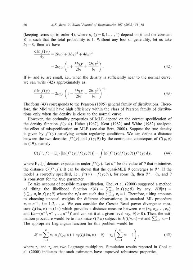
(keeping terms up to order 4), where bj (j=0; 1; : : : ; 4) depend on � and the constantC is such that the total probability is 1. Without any loss of generality, let us takeb1 = 0; then we have
d lnf(y)dy
= 2b2y + 3b3y2 + 4b4y3
= 2b2y(1 +
3b3y2b2
+2b4y2
b2
): (42)
If b3 and b4 are small, i.e., when the density is su<ciently near to the normal curve,we can write (42) approximately as
d lnf(y)dy
= 2b2y(1− 3b3y
2b2− 2b4y2
b2
)−1
: (43)
The form (43) corresponds to the Pearson (1895) general family of distributions. There-fore, the MM will have high e<ciency within the class of Pearson family of distribu-tions only when the density is close to the normal curve.However, the optimality properties of MLE depend on the correct speci4cation of
the density function f(y; �). Huber (1967), Kent (1982) and White (1982) analyzedthe eRect of misspeci4cation on MLE (see also Bera, 2000). Suppose the true densityis given by f∗(y) satisfying certain regularity conditions. We can de4ne a distancebetween the two densities f∗(y) and f(y; �) by the continuous counterpart of C(p; q)in (19), namely
C(f∗; f) = Ef∗ [ln(f∗(y)=f(y; �))] =∫
ln(f∗(y)=f(y; �))f∗(y) dy; (44)
where Ef∗ [·] denotes expectation under f∗(y). Let � ∗ be the value of � that minimizesthe distance C(f∗; f). It can be shown that the quasi-MLE � converges to � ∗. If themodel is correctly speci4ed, i.e., f∗(y) = f(y; �0), for some �0, then � ∗ = �0, and �is consistent for the true parameter.To take account of possible misspeci4cation, Choi et al. (2000) suggested a method
of tilting the likelihood function ‘(�) =∑n
i=1 lnf(yi; �) by say, ‘(�|�) =∑ni=1 �i lnf(yi; �) where the �i’s are such that
∑ni=1 �i=1. Therefore, tilting amounts
to choosing unequal weights for diRerent observations; in standard ML procedure�i = n−1; i = 1; 2; : : : ; n. We can consider the Cressie–Read power divergence mea-sure I�(i=n; �) in (14) which provides a distance measure between �= (�1; �2; : : : ; �n)′
and i=n=(n−1; n−1; : : : ; n−1)′ and can set it at a given level say, �(¿ 0). Then, the esti-mation procedure would be to maximize ‘(�|�) subject to I�(i=n; �)=� and
∑ni=1 �i=1.
The appropriate Lagrangian function for this problem would be
L=n∑i=1
�i lnf(yi; �) + /1(I�(i=n; �)− �) + /2
(n∑i=1
�i − 1
); (45)
where /1 and /2 are two Lagrange multipliers. Simulation results reported in Choi etal. (2000) indicates that such estimators have improved robustness properties.

A.K. Bera, Y. Bilias / Journal of Econometrics 107 (2002) 51–86 67
The optimality of MLE rests on the assumption that we know the true underlyingdensity function. Of course, in econometrics that is rarely the case. Therefore, it isnot surprising that recently econometricians are 4nding the generalized MM (GMM)procedure, which is an extension of Pearson’s MM approach, more attractive. A similarvenue was initiated around 1960s in the statistics literature with the estimating functions(EF) approach to optimal estimation. In some sense, the developments in statistics andeconometrics has come full circle—after discarding the moment approach in favor ofFisher’s maximum likelihood for more than a half century, Karl Pearson’s century-oldtechniques are now found to be more useful in a world with limited information. Whenwe discuss the GMM approach we also present its relation to minimum �2-method.
4. Estimating functions
Durbin (1960) appears to be the 4rst instance of the modern use of “estimatingequations” in econometrics. Durbin’s treatment was amazingly complete. At that timenothing was known, not even asymptotically, about the sampling distributions of theleast squares estimators in the presence of lagged dependent variables among the pre-dictors; a case where the 4nite sample Gauss–Markov theorem is inapplicable. Durbinobserved that the equations from which we obtain the estimators as their roots, eval-uated at the true parameters, preserve their unbiasedness. Thus, it is natural to expectsome sort of optimality properties to be associated with the least squares estimators inthis case as well!To illustrate, let us consider the AR(1) model for yt
yt = �yt−1 + ut ; ut ∼ iid(0; �2); t = 1; : : : ; n:
The least squares estimator of �, �=∑
ytyt−1=∑
y2t−1 is the root of the equation
g(y; �) =∑
ytyt−1 − �∑
y2t−1 = 0; (46)
where y denotes the sample data. The function g(y; �) in (46) is linear in the parameter� and E[g(y; �)] = 0. Durbin (1960) termed g(y; �) = 0 an unbiased linear estimatingequation. Such a class of estimating functions can be denoted by
g(y; �) = T1(y) + �T2(y); (47)
where T1(y) and T2(y) are functions of the data only. Then, Durbin proceeded tode4ne a minimum variance requirement for the unbiased linear estimating functionreminiscent of the Gauss–Markov theorem. As it is possible to change its variance bymultiplying with an arbitrary constant without aRecting the estimator, it seems properto standardize the estimating function by dividing through by E(T2(y)), which is notbut E(@g=@�).Durbin (1960) turned into the study of estimating functions as a means of studying
the least squares estimator itself. In Durbin’s context, let t1 = T1(y)=E(T2(y)), t2 =T2(y)=E(T2(y)), and write
gs(y; �) = t1 + �t2

68 A.K. Bera, Y. Bilias / Journal of Econometrics 107 (2002) 51–86
for the standardized linear estimating function. For the root of the equation t1+ �t2=0,we can write:
t2(�− �) =−(t1 + �t2) (48)
which indicates that the sampling error of the estimator depends on the properties of theestimating function. Clearly, it is more convenient to study a linear function and thentransfer its properties to its non-linear root instead of studying directly the estimatoritself. Durbin used representation (48) to study the asymptotic properties of the leastsquares estimator when lagged dependent variables are included among the regressors.More generally, a 4rst-order Taylor series expansion of g(�) = 0 around �,
n1=2(�− �) ≈ −n−1=2g(�)×(n−1 @g
@�
)−1
≈ −n1=2g(�)×[E(@g@�
)]−1
;
indicates that in order to obtain an estimator with minimum limiting variance, theestimating function g has to be chosen with minimum variance of its standardizedform, g(�)× [E(@g(�)=@�)]−1.Let G denote a class of unbiased estimating functions. Let
gs =g
E[@g=@�](49)
be the standardized version of the estimating function g∈G. We will say that g∗ isthe best unbiased estimating function in the class G, if and only if, its standardizedversion has minimum variance Var(g∗s ) in the class; that is
Var(g∗s )6Var(gs) for all other g∈G: (50)
This optimality criterion was suggested by Godambe (1960) for general classes of esti-mating functions and, independently, by Durbin (1960) for linear classes of estimatingfunctions de4ned in (47). The motivation behind the Godambe–Durbin criterion (50)as a way of choosing from a class of unbiased estimating functions is intuitively sound:it is desirable that g is as close as possible to zero when it is evaluated at the truevalue � which suggests that we want Var(g) to be as small as possible. At the sametime we want any deviation from the true parameter to lead g as far away from zeroas possible, which suggests that [E(@g=@�)]2 be large. These two goals can be accom-plished simultaneously with the Godambe–Durbin optimality criterion that minimizesthe variance of gs in (49).These developments can be seen as an analog of the Gauss–Markov theory for
estimating equations. Moreover, let ‘(�) denote the loglikelihood function and diRer-entiate E[g(y; �)] = 0 to obtain E[@g=@�] =−Cov[g; @‘(�)=@�]. Squaring both sides ofthis equality and applying the Cauchy–Schwarz inequality yields the CramUer–Rao typeinequality
E(g2)
[E(@g=@�)]2¿
1E[(@‘(�)=@�)2]
; (51)
for estimating functions. Thus, a lower bound, given by the inverse of the informa-tion matrix of the true density f(y; �), can be obtained for Var(g). Based on (51),

A.K. Bera, Y. Bilias / Journal of Econometrics 107 (2002) 51–86 69
Godambe (1960) concluded that for every sample size, the score @‘(�)=@� is theoptimum estimating function. Concurrently, Durbin (1960) derived this result for theclass of linear estimating equations. It is worth stressing that it provides an exact or4nite sample justi4cation for the use of maximum likelihood estimation. Recall thatthe usual justi4cation of the likelihood-based methods, when the starting point is theproperties of the estimators, is asymptotic, as discussed in Section 3. A related resultis that the optimal estimating function within a class G has maximum correlation withthe true score function; cf. Heyde (1997). Since the true loglikelihood is rarely known,this result is more useful from practical point of view.Many other practical bene4ts can be achieved when working with the estimating
functions instead of the estimators. Estimating functions are much easier to combineand they are invariant under one-to-one transformations of the parameters. Finally, theapproach preserves the spirit of the method of moments estimation and it is well suitedfor semiparametric models by requiring only assumptions on a few moments.
Example 1. The estimating function (46) in the AR(1) model can be obtained in analternative way that sheds light to the distinctive nature of the theory of estimatingfunctions. Since E(ut) = 0; ut = yt − �yt−1; t = 1; 2; : : : ; n are n elementary estimatingfunctions. The issue is how we should combine the n available functions to solve for thescalar parameter �. To be more speci4c; let ht be an elementary estimating function ofy1; y2; : : : ; yt and �; with Et−1(ht) ≡ E(ht |y1; : : : ; yt−1)=0. Then; by the law of iteratedexpectations E(hsht) = 0 for s �= t. Consider the class of estimating functions g
g=n∑t=1
at−1ht
created by using diRerent weights at−1; which are dependent only on the conditioningevent (here; y1; : : : ; yt−1). It is clear that; due to the law of iterated expectations;E(g) = 0. In this class; Godambe (1985) showed that the quest for minimum varianceof the standardized version of g yields the formula for the optimal weights as
a∗t−1 =Et−1(@ht=@�)Et−1(h2t )
: (52)
Application of (52) in the AR(1) model gives a∗t−1 = −yt−1=�2; and so the optimalestimating equation for � is
g∗ =n∑t=1
yt−1(yt − �yt−1) = 0:
In summary; even if the errors are not normally distributed; the least squares estimatingfunction has some optimum quali4cations once we restrict our attention to a particularclass of estimating functions.Example 1 can be generalized further. Consider the scalar dependent variable yi with
expectation E(yi)=i(�) modeled as a function of a p×1 parameter vector �; the vectorof explanatory variables xi; i = 1; : : : ; n is omitted for convenience. Assume that theyi’s are independent with variances Var(yi) possibly dependent on �. Then, the optimal
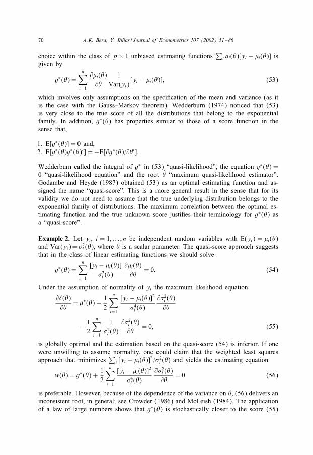
70 A.K. Bera, Y. Bilias / Journal of Econometrics 107 (2002) 51–86
choice within the class of p× 1 unbiased estimating functions∑
i ai(�)[yi − i(�)] isgiven by
g∗(�) =n∑i=1
@i(�)@�
1Var(yi)
[yi − i(�)]; (53)
which involves only assumptions on the speci4cation of the mean and variance (as itis the case with the Gauss–Markov theorem). Wedderburn (1974) noticed that (53)is very close to the true score of all the distributions that belong to the exponentialfamily. In addition, g∗(�) has properties similar to those of a score function in thesense that,
1. E[g∗(�)] = 0 and,2. E[g∗(�)g∗(�)′] =−E[@g∗(�)=@�′].
Wedderburn called the integral of g∗ in (53) “quasi-likelihood”, the equation g∗(�) =0 “quasi-likelihood equation” and the root � “maximum quasi-likelihood estimator”.Godambe and Heyde (1987) obtained (53) as an optimal estimating function and as-signed the name “quasi-score”. This is a more general result in the sense that for itsvalidity we do not need to assume that the true underlying distribution belongs to theexponential family of distributions. The maximum correlation between the optimal es-timating function and the true unknown score justi4es their terminology for g∗(�) asa “quasi-score”.
Example 2. Let yi; i = 1; : : : ; n be independent random variables with E(yi) = i(�)and Var(yi)=�2i (�); where � is a scalar parameter. The quasi-score approach suggeststhat in the class of linear estimating functions we should solve
g∗(�) =n∑i=1
[yi − i(�)]�2i (�)
@i(�)@�
= 0: (54)
Under the assumption of normality of yi the maximum likelihood equation
@‘(�)@�
= g∗(�) +12
n∑i=1
[yi − i(�)]2
�4i (�)@�2i (�)@�
− 12
n∑i=1
1�2i (�)
@�2i (�)@�
= 0; (55)
is globally optimal and the estimation based on the quasi-score (54) is inferior. If onewere unwilling to assume normality; one could claim that the weighted least squaresapproach that minimizes
∑i [yi − i(�)]2=�2i (�) and yields the estimating equation
w(�) = g∗(�) +12
n∑i=1
[yi − i(�)]2
�4i (�)@�2i (�)@�
= 0 (56)
is preferable. However; because of the dependence of the variance on �; (56) delivers aninconsistent root; in general; see Crowder (1986) and McLeish (1984). The applicationof a law of large numbers shows that g∗(�) is stochastically closer to the score (55)

A.K. Bera, Y. Bilias / Journal of Econometrics 107 (2002) 51–86 71
than is w(�). In a way; the second term in (56) creates a bias in w(�); and the thirdterm in (55) “corrects” for this bias in the score equation. Here; we have a case inwhich the extremum estimator (weighted least squares) is inconsistent; while the rootof the quasi-score estimating function is consistent and optimal within a certain classof estimating functions.The theory of estimating functions has been extended to numerous other directions.
For extensions to dependent responses and optimal combination of higher-order mo-ments, see Heyde (1997) and the citations therein. For various applications see thevolume edited by Godambe (1991) and Vinod (1998). Li and Turtle (2000) oRered anapplication of the EF approach in the ARCH models.
5. Modern approaches to estimation in econometrics
Pressured by the complicity of econometric models, econometricians looked for meth-ods of estimation that bypass the use of likelihood. This trend was also supported bythe nature of economic theories that do provide characterization of the stochastic lawsonly in terms of moment restrictions; see Hall (2001) for speci4c examples. In the fol-lowing we describe the instrumental variables (IV) estimator, the generalized methodof moments (GMM) estimator and some recent extensions of GMM based on em-pirical likelihood. Often, the 4rst instances of these methods appear in the statisticalliterature. However, econometricians, faced with the challenging task of estimating eco-nomic models, also oRered new and interesting twists. We start with Sargan’s (1958)IV estimation.The use of IV was 4rst proposed by ReiersHl (1941, 1945) as a method of consistent
estimation of linear relationships between variables that are characterized by measure-ment error. 19 Subsequent developments were made by Geary (1948, 1949) and Durbin(1954). A de4nite treatment of the estimation of linear economic relationships usinginstrumental variables was presented by Sargan (1958, 1959).In his seminal work, Sargan (1958) described the IV method as it is used currently
in econometrics, derived the asymptotic distribution of the estimator, solved the prob-lem of utilizing more instrumental variables than the regressors to be instrumentedand discussed the similarities of the method with other estimation methods availablein the statistical literature. This general theory was applied to time series data withautocorrelated residuals in Sargan (1959).In the following we will use x to denote a regressor that is possibly subjected to
measurement error and z to denote an instrumental variable. It is assumed that a linearrelationship holds,
yi = 71x1i + · · ·+ 7pxpi + ui; i = 1; : : : ; n; (57)
19 The history of IV estimation goes further back. In a series of work Wright (1920, 1921, 1925, 1928)advocated a graphical approach to estimate simultaneous equation systems what he referred to as “pathanalysis”. In his 1971 Schultz Lecture, Goldberger (1972, p. 938) noted: “Wright drew up a Zow chart,: : : and read oR the chart a set of equations in which zero covariances are exploited to express momentsamong observable variables in terms of structural parameters. In eRect, he read oR what we might now callinstrumental-variable estimating equations”. For other related references see Manski (1988, p. xii).

72 A.K. Bera, Y. Bilias / Journal of Econometrics 107 (2002) 51–86
where the residual u in (57) includes a linear combination of the measurement errorsin x’s. In this case, the method of least squares yields inconsistent estimates of theparameter vector. ReiersHl’s (1941; 1945) method of obtaining consistent estimates isequivalent to positing a zero sample covariance between the residual and each instru-mental variable. Then, we obtain p equations,
∑ni=1 zkiui = 0; k = 1; : : : ; p, on the p
parameters; the number of available instrumental variables is assumed to be equal tothe number of regressors.It is convenient to express ReiersHl’s methodology in matrix form. Let Z be a (n×q)
matrix of instrumental variables with kth column z′k=(zk1; zk2 : : : ; zkn)′, and for the timebeing we take q=p. Likewise X is the (n×p) matrix of regressors, u the n×1 vectorof residuals and y the n× 1 vector of responses. Then, the p estimating equations canbe written more compactly as
Z ′u= 0 or Z ′(y − X7) = 0; (58)
from which the simple IV estimator, 7 = (Z ′X )−1Z ′y, follows. Under the assump-tions that (i) plim n−1Z ′Z = :ZZ , (ii) plim n−1Z ′X = :ZX , and (iii) n−1=2Z ′u tends indistribution to a normal vector with mean zero and covariance matrix �2:ZZ , it canbe concluded that the simple IV estimator 7 has a normal limiting distribution withcovariance matrix Var(n1=27) = �2:−1
ZX :ZZ:−1XZ (see Hall, 1993).
ReiersHl’s method of obtaining consistent estimates can be classi4ed as an applicationof the Pearson’s MM procedure. 20 Each instrumental variable z induces the momentrestriction E(zu) = 0. In ReiersHl’s work, which Sargan (1958) developed rigorously,the number of these moment restrictions that the data satisfy are equal to the numberof unknown parameters. A major accomplishment of Sargan (1958) was the study ofthe case in which the number of available instrumental variables is greater than thenumber of regressors to be instrumented. Any subset of p instrumental variables canbe used to to form p equations for the consistent estimation of the p parameters.Sargan (1958, pp. 398–399) proposed that, p linear combinations of the instrumentalvariables are constructed with the weights chosen so as to minimize the covariancematrix of asymptotic distribution. More generally, if the available number of momentrestrictions exceeds that of the unknown parameters, p (optimal) linear combinations ofthe moments can be used for estimation. This idea pretty much paved the way for the
20 There is also a connection between the IV and the limited information maximum likelihood (LIML)procedures which generally is not mentioned in the literature. Interviewed in 1985 for the 4rst issue ofthe Econometric Theory, Dennis Sargan recorded this connection as his original motivation. Around 1950sSargan was trying to put together a simple Klein-type model for the UK, and his attempt to estimate thismacroeconomic model led him to propose the IV method of estimation as he stated (see Phillips, 1985,p. 123): “At that stage I also became interested in the elementary methods of estimation and stumbledupon the method of instrumental variables as a general approach. I did not become aware of the CowlesFoundation results, particularly the results of Anderson and Rubin on LIML estimation until their work waspublished in the late 1940s. I realized it was very close to instrumental variable estimation. The article whichstarted me up was the article by Geary which was in the JRSS in 1948. That took me back to the earlierwork by ReiersHl, and I pretty early realized that the Geary method was very close to LIML except he wasusing arbitrary functions of time as the instrumental variables, particularly polynomials in the time variable.One could easily generalize the idea to the case, for example, of using lagged endogenous variables togenerate the instrumental variables. That is really where my instrumental variable estimation started from”.

A.K. Bera, Y. Bilias / Journal of Econometrics 107 (2002) 51–86 73
more recent advances of the GMM approach in the history of econometric estimationand the testing of overidentifying restrictions. As we show earlier, the way that the EFapproach to optimal estimation proceeds is very similar.Speci4cally, suppose that there are q(¿p) instrumental variables from which we
construct a reduced set of p variables z∗ki,
z∗ki =q∑
j=1
�kjzji; i = 1; : : : ; n; k = 1; : : : ; p:
Let us, for ease of notation, illustrate the solution to this problem using matrices. Forany (q×p) weighting matrix �= [�kj] with rank[�] =p; Z∗ = Z� produces a new setof p instrumental variables. Using Z∗ in the formula of simple IV estimator we obtainan estimator of 7 with asymptotic distribution
√n(7 − 7) d→N (0; �2(�′:ZX )−1(�′:ZZ�)(:XZ�)−1): (59)
The next question is, which matrix � yields the minimum asymptotic variance–covariance matrix. It can be shown that the optimal linear combination of the q instru-mental variables is the one that maximizes the correlation of Z∗ with the regressorsX . Since the method of least squares maximizes the squared correlation between thedependent variable and its 4tted value, the optimal (q × p) matrix � = [�kj] is foundto be �0 = :−1
ZZ :ZX , for which it is checked that
06 [�(:XZ�)−1 − �0(:XZ�0)−1]′:ZZ [�(:XZ�)−1 − �0(:XZ�0)−1]
= (�′:ZX )−1�′:ZZ�(:XZ�)−1 − (�′0:ZX )−1�′0:ZZ�0(:XZ�0)−1: (60)
In practice, �0 is consistently estimated by �0=(Z ′Z)−1Z ′X and the proposed optimalinstrumental matrix is consistently estimated by the 4tted value from regressing X onZ ,
Z∗0 = Z�0 = Z(Z ′Z)−1Z ′X ≡ X : (61)
Then, the instrumental variables estimation methodology applies as before with Z∗0 ≡ X
as the set of instrumental variables. The set of estimating equations (58) is replacedby X
′u= 0 which in turn yields
7 = (X′X )−1X
′y (62)
with covariance matrix of the limiting distribution Var(n1=27)=�2(:XZ:−1ZZ :ZX )−1. This
estimator is termed generalized IV estimator as it uses the q(¿p) available momentsE(zju)=0; j=1; 2; : : : ; q for estimating the p-vector parameter 7. While Sargan (1958)combined the q instrumental variables to form a new composite instrumental variable,the same result can be obtained using the sample analogs of q moments themselves.This brings us back to the minimum �2 and the GMM approaches to estimation.
The minimum �2 method and diRerent variants are reviewed in Ferguson (1958). Hisarticle also includes a new method of generating best asymptotically normal (BAN)estimates. These methods are extremely close to what is known today in econometricsas the GMM. A recent account is provided by Ferguson (1996). To illustrate, let us
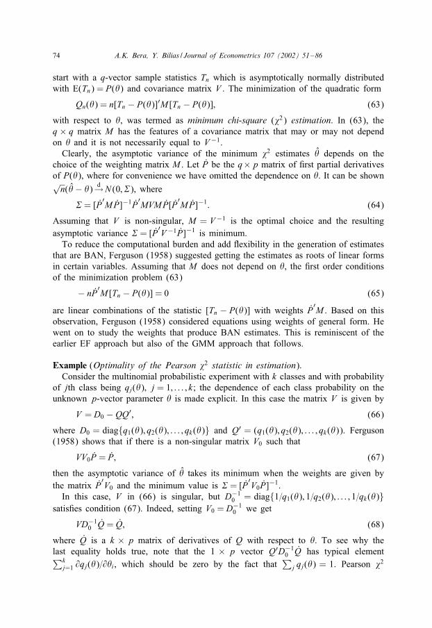
74 A.K. Bera, Y. Bilias / Journal of Econometrics 107 (2002) 51–86
start with a q-vector sample statistics Tn which is asymptotically normally distributedwith E(Tn) = P(�) and covariance matrix V . The minimization of the quadratic form
Qn(�) = n[Tn − P(�)]′M [Tn − P(�)]; (63)
with respect to �, was termed as minimum chi-square (�2) estimation. In (63), theq × q matrix M has the features of a covariance matrix that may or may not dependon � and it is not necessarily equal to V−1.Clearly, the asymptotic variance of the minimum �2 estimates � depends on the
choice of the weighting matrix M . Let P be the q×p matrix of 4rst partial derivativesof P(�), where for convenience we have omitted the dependence on �. It can be shown√n(�− �) d→N (0; :), where
:= [P′MP]−1P
′MVMP[P
′MP]−1: (64)
Assuming that V is non-singular, M = V−1 is the optimal choice and the resultingasymptotic variance := [P
′V−1P]−1 is minimum.
To reduce the computational burden and add Zexibility in the generation of estimatesthat are BAN, Ferguson (1958) suggested getting the estimates as roots of linear formsin certain variables. Assuming that M does not depend on �, the 4rst order conditionsof the minimization problem (63)
− nP′M [Tn − P(�)] = 0 (65)
are linear combinations of the statistic [Tn − P(�)] with weights P′M . Based on this
observation, Ferguson (1958) considered equations using weights of general form. Hewent on to study the weights that produce BAN estimates. This is reminiscent of theearlier EF approach but also of the GMM approach that follows.
Example (Optimality of the Pearson �2 statistic in estimation):Consider the multinomial probabilistic experiment with k classes and with probability
of jth class being qj(�); j = 1; : : : ; k; the dependence of each class probability on theunknown p-vector parameter � is made explicit. In this case the matrix V is given by
V = D0 − QQ′; (66)
where D0 = diag{q1(�); q2(�); : : : ; qk(�)} and Q′ = (q1(�); q2(�); : : : ; qk(�)). Ferguson(1958) shows that if there is a non-singular matrix V0 such that
VV0P = P; (67)
then the asymptotic variance of � takes its minimum when the weights are given bythe matrix P
′V0 and the minimum value is := [P
′V0P]−1.
In this case, V in (66) is singular, but D−10 = diag{1=q1(�); 1=q2(�); : : : ; 1=qk(�)}
satis4es condition (67). Indeed, setting V0 = D−10 we get
VD−10 Q = Q; (68)
where Q is a k × p matrix of derivatives of Q with respect to �. To see why thelast equality holds true, note that the 1 × p vector Q′D−1
0 Q has typical element∑kj=1 @qj(�)=@�i, which should be zero by the fact that
∑j qj(�) = 1. Pearson �2

A.K. Bera, Y. Bilias / Journal of Econometrics 107 (2002) 51–86 75
statistic uses precisely V0 =D−10 and therefore the resulting estimators are e<cient [see
Eq. (11)]. Pearson �2 statistic is an early example of the optimal GMM approach toestimation.
Ferguson (1958) reformulated the minimum �2 estimation problem in terms of esti-mating equations. By interpreting the 4rst order conditions of the problem as a linearcombination of elementary estimating functions, he realized that the scope of consistentestimation can be greatly enhanced. In econometrics, Goldberger (1968, p. 4) suggestedthe use of “analogy principle of estimation” as a way of forming the normal equationsin the regression problem. However, the use of this principle (or MM) instead of theleast squares was not greatly appreciated at that time. 21 It was only with GMM thateconometricians gave new force to the message delivered by Ferguson (1958) and real-ized that IV estimation can be considered as a special case of a more general approach.Hansen (1982) looked on the problem of consistent estimation from the MM point ofview. 22 For instance, assuming that the covariance of each instrumental variable withthe residual is zero provided that the parameter is at its true value, the sample analogof the covariance will be a consistent estimator of zero. Therefore, the root of theequation that equates sample covariance to zero should be close to the true parameter.On the contrary, in the case of regressors subjected to measurement errors, the normalequations X ′u = 0 will fail to produce consistent estimates because the correspondingpopulation moment condition is not zero.Let h(y; �) be a general (q× 1) function of data y and p-vector parameter �, with
the property that for �= �0
E[h(y; �0)] = 0: (69)
We say that the function h(y; �) satis4es a moment or an orthogonality conditionthat holds true only when � is at its true value �0. Alternatively, there are q momentconditions that can be used to determine an estimate of the p-vector �0. If q=p then
g(�) ≡ 1n
n∑i=1
h(yi; �) = 0
will yield roots � that are unique parameter estimates.
21 In reviewing Goldberger (1968), Katti (1970) commented on the analogy principle as: “This is cute andwill help one remember the normal equations a little better. There is no hint in the chapter—and I believeno hints exist—which would help locate such criteria in other situations, for example, in the problem ofestimating the parameters in the gamma distribution. Thus, this general looking method has not been shownto be capable of doing anything that is not already known. Ad hoc as this method is, it is of course di<cultto prove that the criteria so obtained are unique or optimal”. Manski (1988, p. ix) acknowledged that hebecame aware of Goldberger’s analogy principle only in 1984 when he started writing his book.22 From our conversation with Lars Hansen and Christopher Sims, we learned that a rudimentary form
of GMM estimator existed in Sims’ lecture notes. Hansen attended Sims’ lectures as a graduate studentat the University of Minnesota. Hansen formally wrote up the theories of GMM estimator and found itsclose connection to Sargan’s (1958) IV estimator. To diRerentiate his paper, Hansen used a very generalframework and established the properties of the estimator under mild assumptions. In the econometricsliterature, Hansen (1982) has been the most inZuential paper to popularize the moment type and minimum�2 estimation techniques.
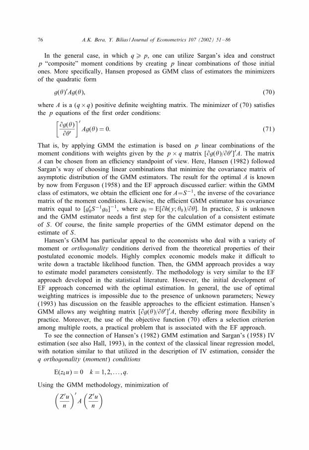
76 A.K. Bera, Y. Bilias / Journal of Econometrics 107 (2002) 51–86
In the general case, in which q¿p, one can utilize Sargan’s idea and constructp “composite” moment conditions by creating p linear combinations of those initialones. More speci4cally, Hansen proposed as GMM class of estimators the minimizersof the quadratic form
g(�)′Ag(�); (70)
where A is a (q×q) positive de4nite weighting matrix. The minimizer of (70) satis4esthe p equations of the 4rst order conditions:[
@g(�)@�′
]′Ag(�) = 0: (71)
That is, by applying GMM the estimation is based on p linear combinations of themoment conditions with weights given by the p× q matrix [@g(�)=@�′]′A. The matrixA can be chosen from an e<ciency standpoint of view. Here, Hansen (1982) followedSargan’s way of choosing linear combinations that minimize the covariance matrix ofasymptotic distribution of the GMM estimators. The result for the optimal A is knownby now from Ferguson (1958) and the EF approach discussed earlier: within the GMMclass of estimators, we obtain the e<cient one for A=S−1, the inverse of the covariancematrix of the moment conditions. Likewise, the e<cient GMM estimator has covariancematrix equal to [g′0S
−1g0]−1, where g0 = E[@h(y; �0)=@�]. In practice, S is unknownand the GMM estimator needs a 4rst step for the calculation of a consistent estimateof S. Of course, the 4nite sample properties of the GMM estimator depend on theestimate of S.Hansen’s GMM has particular appeal to the economists who deal with a variety of
moment or orthogonality conditions derived from the theoretical properties of theirpostulated economic models. Highly complex economic models make it di<cult towrite down a tractable likelihood function. Then, the GMM approach provides a wayto estimate model parameters consistently. The methodology is very similar to the EFapproach developed in the statistical literature. However, the initial development ofEF approach concerned with the optimal estimation. In general, the use of optimalweighting matrices is impossible due to the presence of unknown parameters; Newey(1993) has discussion on the feasible approaches to the e<cient estimation. Hansen’sGMM allows any weighting matrix [@g(�)=@�′]′A, thereby oRering more Zexibility inpractice. Moreover, the use of the objective function (70) oRers a selection criterionamong multiple roots, a practical problem that is associated with the EF approach.To see the connection of Hansen’s (1982) GMM estimation and Sargan’s (1958) IV
estimation (see also Hall, 1993), in the context of the classical linear regression model,with notation similar to that utilized in the description of IV estimation, consider theq orthogonality (moment) conditions
E(zku) = 0 k = 1; 2; : : : ; q:
Using the GMM methodology, minimization of(Z ′un
)′A(Z ′un
)
A.K. Bera, Y. Bilias / Journal of Econometrics 107 (2002) 51–86 77
with respect to 7, in view of u= y − X7, yields 4rst order conditions
− 2X ′ZAZ ′(y − X7) = 0: (72)
If q = p, then (72) reduces to (58) which yields the simple IV estimator. Clearly, incase the orthogonality conditions are equal to the number of unknown parameters, the7 is just identi4ed and the choice of the weighting matrix A is inconsequential.If q¿p, the p×q matrix X ′ZA in (72) transforms the q (sample) moments Z ′(y−
X 7) into p linear combinations that can be used to produce a unique solution for 7.Now, diRerent choices of A will yield consistent estimates with diRerent asymptoticvariances. The discussion earlier suggests that, in order to attain e<ciency with thegiven set of q orthogonality conditions, beyond a constant of proportionality, we shouldpick A = :−1
ZZ ; in practice the consistent estimate (n−1Z ′Z)−1 will be utilized. Withthat choice for A, the GMM estimator is identical to Sargan’s generalized IV estimator(62). Now we turn our discussion to empirical likelihood (EL)-based estimation thathas recently become popular in econometrics.In practice, inference based on the GMM as suggested by Hansen (1982) and its
asymptotically equivalent forms suRers from poor 4nite sample properties; see for in-stance, Hansen et al. (1996) and, Pagan and Robertson (1997). The EL method pro-posed by Owen (1988) has been fruitfully adapted to oRer an alternative approachto inference in econometric models: the empirical likelihood is maximized subject tothe moment restrictions that data satisfy in the population. ERectively, these methodsimpose the moment restrictions by appropriately reweighting the data. The resultingestimator of the unknown parameter is 4rst-order asymptotically equivalent to the e<-cient GMM estimator. Moreover, the sampling properties of the estimators are similarto those supported by bootstrap, thus oRering an increased chance of 4nite-sampleproperties that are in accordance with asymptotic theory.Let � be the unknown parameter of primary interest. The moment condition
E[h(y; �)] = 0 holds at �0, the true value of the parameter. Qin and Lawless (1994)proposed estimating the parameter � by solving the problem:
max�i;�
n∑i=1
ln �i s:t:n∑i=1
�i = 1;n∑i=1
�ih(yi; �) = 0; (73)
where each �i is restricted to be non-negative. This is equivalent to minimizing the en-tropy measure (18) satisfying given moment conditions. The restriction
∑i �ih(yi; �)=0
can be interpreted as the empirical analog of the moment condition with �i being theprobability of the random variable y to take the value yi. This empirical analog dif-fers from the one that is used in the classical MM (or Hansen’s GMM) in that inthe latter we assume �i = n−1 for every observation yi. In the absence of the momentrestriction
∑i �ih(yi; �)=0 the above optimization program is the non-parametric max-
imum log-likelihood that has the solution �i = n−1; each sample observation is equallyweighted. In the presence of the constraint the diRerentiation of the Lagrangian function
L=n∑i=1
ln �i +
(1−
n∑i=1
�i
)− n/′
n∑i=1
�ih(yi; �) (74)

78 A.K. Bera, Y. Bilias / Journal of Econometrics 107 (2002) 51–86
yields estimated probabilities
�el; i =1
n[1 + /′elh(yi; �el)]: (75)
The estimated probabilities (75) diRer from the uniform distribution, which assigns toeach observation equal weight n−1, to the degree that the Lagrange multiplier vector ofthe moment restriction /el, or tilting parameter, is away from zero or to the degree thatthe moment restriction hold true. The EL approach for parameter estimation works by4nding the multinomial distribution (or, alternatively, the empirical probability distribu-tion) �=(�1; �2; : : : ; �n) that accommodates the moment conditions. Now, the estimatedprobabilities are functions of �.Manipulation of the 4rst-order conditions from the Lagrangian (74) gives an al-
ternative characterization of the solution (�el; /el) that connects with the estimatingfunction approach. The estimators satisfy the equations
∑ni=1 (el(yi; �el; /el) = 0,
where
(el(y; �; /) =
/′
@h(y; �)@�′
[1 + /′h(y; �)]−1
h(y; �)[1 + /′h(y; �)]−1
: (76)
The dimension of the multiplier / is equal to the number of moment conditions givenby the dimension of the function h(y; �). It can be shown that, under regularity condi-tions and for the given set of moment conditions, �el is asymptotically equivalent to thee<cient estimator within the class of the GMM estimators. The e<cient GMM estima-tor usually necessitates a two-step procedure for the estimation of the best weightingmatrix. In contrast, the empirical likelihood approach requires only one-step, and thisis expected to result in improved 4nite-sample properties of estimators [see for ex-ample, Mittelhammer and Judge (2001)]. In other words, as it is also emphasized inMittelhammer et al. (2000, Chapter 12), the empirical likelihood approach oRers anoperational way to optimally combine estimating equations.Golan and Judge (1996), Imbens (1997), Imbens et al. (1998), and, Qin and Lawless
(1994) proposed a diRerent objective function motivated by entropy or the Kullback–Leibler information criterion (KLIC). This suggestion leads to the so-called exponentialtilting (ET) estimator �et of �, which is based on the optimization problem [see alsoEq. (20) and the discussion that follows]
min�i; �
n∑i=1
�i ln �i s:t:n∑i=1
�i = 1;n∑i=1
�ih(yi; �) = 0: (77)
We denote the estimated Lagrange multiplier for the moment restrictions by /et. Again,the solution yields estimated probabilities that are diRerent from n−1:
�et; i =exp{/′eth(yi; �et)}∑ni=1 exp{/′eth(yi; �et)}
: (78)
A.K. Bera, Y. Bilias / Journal of Econometrics 107 (2002) 51–86 79
The estimators in this problem satisfy the estimating equations∑n
i=1 (et(yi; �et ; /et)=0,where
(et(y; �; /) =
/′
@h(y; �)@�′
exp{/′h(yi; �)}h(y; �) exp{/′h(yi; �)}
: (79)
The ET estimator was also suggested by Kitamura and Stutzer (1997) who handlethe important case of weakly dependent data. Their proposal utilizes the frameworkof linear inverse problems and that allows them to propose convenient computationalprocedures. They show that the ET estimators for (�; /) can be characterized by theoptimization program
(�et ; /et) = argmax�
min/
n∑i=1
exp{/′h(yi; �)}: (80)
From (80), it is easy to obtain the estimating functions given by (79). Similar charac-terization can be made for the EL problem thereby yielding the set of just identi4edEq. (76).In the case of serially correlated observations Kitamura and Stutzer (1997) propose
to smooth the observations before the optimization and, in particular, to replace h(yi; �)in (80) by
Qhi(�) =K∑
k=−K
12K + 1
h(yi−k ; �);
where K2=n → 0, and K → ∞ as n → ∞.The limiting distributions of the EL estimator �el and the ET estimator �et are iden-
tical; see Imbens et al. (1998). They are both√n-consistent and asymptotically normal
N (0; :), where
:={E(@h(y; �0)
@�
)[E(h(y; �0)h(y; �0)′)]−1E
(@h(y; �0)
@�
)}−1
; (81)
where the expectations are evaluated at the true value of parameter �0. A consistentestimate of : can be constructed by using the empirical analogs of each expecta-tion involved. E<ciency dictates that each observation yi is weighted by the esti-mated probability �i. For instance, when working with the exponential tilting estimatorE(h(y; �0)h(y; �0)′) will be estimated by
∑i �et; ih(yi; �et)h(yi; �et)
′. However, consis-tency is not lost by using the uniform weights n−1.Imbens et al. (1998) also show that the two estimators can be nested in a class
of estimators that arise from the minimization of the Cressie–Read power-divergencecriterion (14) (Cressie and Read, 1984; Read and Cressie, 1988). Consider two discretedistributions with common support p = (p1; p2; : : : ; pn) and q = (q1; q2; : : : ; qn) andrewrite the Cressie–Read power-divergence criterion as
I�(p; q) =1
�(1 + �)
n∑i=1
pi
[(pi
qi
)�− 1
]; (82)
80 A.K. Bera, Y. Bilias / Journal of Econometrics 107 (2002) 51–86
where � is a given constant, and therefore, we can talk about a class of divergencecriteria. For given �, the estimators for � are de4ned so that the distance of the esti-mated probabilities �i from the empirical distribution n−1 is minimized subject to themoment restrictions. More speci4cally, let pi = n−1 and qi = �i. For 4xed constant �,we consider the minimization program
min�i;�
I�(i=n; �) s:t:n∑i=1
�i = 1;n∑i=1
�ih(yi; �) = 0: (83)
For � → 0, we obtain the empirical likelihood based estimators (�el; �el). When� → −1, the exponential tilting estimators (�et ; �et) arise. It would be an interest-ing problem to combine Choi et al. (2000) empirical tilting model method and theabove empirical likelihood method. A possible optimization problem would be to max-imize
∑ni=1 �i lnf(yi; �) subject to
∑ni=1 �i =1,
∑ni=1 �ih(yi; �)=0 and I�(i=n; �)= �
for given small value of �.An interesting special case of the minimization program (83) is the log Euclidean
likelihood estimator �lel, obtained when � = −2; see Owen (1991), Qin and Lawless(1994). Imbens et al. (1998) show that �lel, for given estimate of the multiplier /, ischaracterized by the estimating equation[
n∑i=1
@h(yi; �lel)@�′
(1 + /′h(yi; �lel))
]′[
n∑i=1
h(y; �lel)h(yi; �lel)′]−1 n∑
i=1
h(yi; �lel) = 0: (84)
When @h(y; �)=@� does not depend on data y, the term (1+ /′h(yi; �)) factors out andthe equation (84) is identical to the one that characterizes the iterated GMM estimator(see Hansen et al., 1996).The characterization of EL and ET by systems of just identi4ed estimating equations,
as well as the fact that GMM can be regarded as a special case of Cressie–Readcriterion, suggest the prevalence of the MM approach to estimation. Manski (1988)included many estimation approaches under the umbrella of analog estimation thatestimates a parameter by the sample analog. In the majority of applications, “sampleanalog” was obtained by equal weighting of each observation. Recent methods haveexpanded the class of analog estimation by stressing e<cient weighting schemes. In ourview it will also be interesting to see how the moment restrictions can be accommodatedin a likelihood framework that is less prone to misspeci4cation of the density function.
6. Epilogue
We have reviewed important phases in the development of parameter estimation, bothin the statistical and econometric literature. We tried to stress the historical continuityof the estimation methodology. In particular, our goal has been towards a synthesisof seemingly unrelated lines of thought. In the light of advancements in the course of
A.K. Bera, Y. Bilias / Journal of Econometrics 107 (2002) 51–86 81
the last century, estimation methods in current use in econometrics do not seem thatdistant from earlier developments in the statistical literature.We started with Pearson’s MM at 1894 and continued with Fisher’s parametric like-
lihood at 1912 and 1922. Based on Pearson’s �2 statistic a third competing methodof estimation was developed under the name “minimum chi-squared”. Subsequently,this statistic provided the basis for the development of a MM approach by Ferguson(1958), that was able to handle cases where the number of available moments ex-ceeds the number of unknown parameters. Parallel lines of research were followed byGodambe (1960) and Durbin (1960) with the estimating function approach. More re-cently, in econometrics Hansen (1982) advocated the GMM procedure that bears closeresemblance to the last two approaches by Ferguson and Godambe–Durbin.Nowadays, econometricians are moving away from the maximum likelihood estima-
tion. The nature of the conclusions derived from economic theorizing and the desire toavoid parametric assumptions push the applied researcher to variants of the method ofmoments. At the onset of the new century, after a long devotion to Fisher’s likelihood,the ideas of Pearson look more useful than ever. It is our view that this interplay be-tween Fisher’s concept of likelihood and Pearson’s method of moments has resulted inan amazing synthesis that provides e<cient estimation with minimal model assumptionsand very promising properties in 4nite samples.These ideas have been blended fruitfully by the non-parametric method of empirical
likelihood. By using the Kullback–Leibler information criterion as a measure of thedistance between two distributions, we can also tie the method of moments to theconcept of entropy. The current state of aRairs calls for more work on these estimationstrategies. Maybe this task also calls for a fresh reading of the old proposals; certainly,the close relationship between modern econometrics with the ideas of Pearson andFisher points to this direction.In this review of the development of estimation, we have occasionally separated
ourselves from the riveting narrative and digressed to some side stories in statistics. Inour view these stories are important. Sometimes seemingly unambiguous description ofdiRerent estimation methodologies in econometrics textbooks brings temporary clarityto our confusions and helps veil some of the parallel, and often-times much earlier,developments in the statistics literature. It is worthwhile to record the initial motiva-tion and historical progress in one place since the original lines of development andphilosophies become clouded by time. Although our overall aim was too ambitious,this paper is essentially our 4rst modest attempt, and some more research along theselines would be pro4table for students of econometrics.
Acknowledgements
We are grateful to Amos Golan and two anonymous referees for many helpful sug-gestions that have considerably improved the paper. An earlier version of this paperunder the title “A Brief History of Estimation” was presented at a conference in honorof George Judge held at the University of Illinois, May 1–2, 1999. We wish to ac-knowledge helpful comments from the participants, in particular, from George Judge
82 A.K. Bera, Y. Bilias / Journal of Econometrics 107 (2002) 51–86
and Arnold Zellner. Kostas Fokianos, Alastair Hall and Yuichi Kitamura kindly pro-vided some extra references and=or detailed comments. We would also like to thankTatyana Dubovyk for providing very competent research assistance and Naoko Miki forher help in preparing the manuscript. Special thanks are due to Amos Golan withoutwhose encouragement and kind prodding the paper would not have been completed.However, we retain the responsibility for any remaining errors. Financial support fromthe O<ce of Research, College of Commerce and Business Administration, Universityof Illinois of Urbana-Champaign (for Anil Bera) and from University of Cyprus (forYannis Bilias) is gratefully acknowledged. This paper is dedicated to George Judge forhis lifelong and continuing contribution to econometrics.
References
Aldrich, J., 1997. R.A. Fisher and the making of maximum likelihood 1912–1922. Statistical Science 12,162–176.
Back, K., Brown, D.P., 1993. Implied probabilities in GMM estimators. Econometrica 61, 971–975.Bennett, T.L., 1907–1908. Errors of observation. Technical Lecture, Number 4, Survey Department, Ministry
of Finance, National Printing Department, Cairo, Egypt.Bera, A.K., 2000. Hypothesis testing in the 20th Century with a special reference to testing with misspeci4ed
models. In: Rao, C.R., Szekely, G.J. (Eds.), Statistics for the 21st Century. Marcel Dekker, New York,pp. 33–92.
Bera, A.K., Bilias, Y., 2000. The MM, ME, ML, EL, EF and GMM approaches to estimation: a synthesis.Working Paper, Department of Economics, University of Illinois.
Bera, A.K., Bilias, Y., 2001. Rao’s score, Neyman’s C(�) and Silvey’s LM tests: an essay on historicaldevelopments and some new results. Journal of Statistical Planning and Inference 97, 9–44.
Bera, A.K., Ghosh, A., 2001. Neyman’s smooth test and its applications in econometrics. In: Ullah, A.,Wan, A., Chaturvedi, A.T. (Eds.), Handbook of Applied Econometrics and Statistical Inference. MarcelDekker, New York, pp. 177–230.
Berger, J.O., 1985. Statistical Decision Theory and Bayesian Analysis. Springer, New York.Berkson, J., 1980. Minimum chi-square, not maximum likelihood! Annals of Statistics 8, 457–487.Box, J.F., 1978. R.A. Fisher: The Life of a Scientist. Wiley, New York.Choi, E., Hall, P., Presnell, B., 2000. Rendering parametric procedures more robust by empirically tilting
the model. Biometrika 87, 453–465.Cressie, N., Read, T.R.C., 1984. Multinomial goodness-of-4t tests. Journal of the Royal Statistical Society.
Series B 46, 440–464.Cowell, F.A., 1980. On the structure of additive inequality measures. Review of Economic Studies 47,
521–531.Crowder, M., 1986. On consistency and inconsistency of estimating equations. Econometric Theory 2, 305–
330.David, H.A., 1995. First (?) occurrence of common terms in mathematical statistics. American Statistician
49, 121–133.Durbin, J., 1954. Errors in variables. Review of Institute of International Statistics 22, 23–54.Durbin, J., 1960. Estimation of parameters in time-series regression models. Journal of the Royal Statistical
Society. Series B 22, 139–153.Edgeworth, F.Y., 1908. On the probable errors of frequency-constants. Journal of the Royal Statistical Society
71, 381–397, 499–512, 651–678.Edgeworth, F.Y., 1909. Addendum on “Probable errors of frequency-constants”. Journal of the Royal
Statistical Society 72, 81–90.Edwards, A.W.F., 1997a. Three early papers on e<cient parametric estimation. Statistical Science 12, 35–47.Edwards, A.W.F., 1997b. What did Fisher mean by ‘inverse probability’ in 1912–1922? Statistical Science
12, 177–184.

A.K. Bera, Y. Bilias / Journal of Econometrics 107 (2002) 51–86 83
Engledow, F.L., Yule, G.U., 1914. The determination of the best value of the coupling-ratio from a givenset of data. Proceedings of the Cambridge Philosophical Society 17, 436–440.
Ferguson, T.S., 1958. A method of generating best asymptotically normal estimates with application toestimation of bacterial densities. Annals of Mathematical Statistics 29, 1046–1062.
Ferguson, T.S., 1996. A Course in Large Sample Theory. Chapman & Hall, London.Fisher, R.A., 1912. On an absolute criterion for 4tting frequency curves. Messenger of Mathematics 41,
155–160.Fisher, R.A., 1921. On the “probable error” of a coe<cient of correlation deduced from a small sample.
Metron 1, 3–32.Fisher, R.A., 1922. On the mathematical foundations of theoretical statistics. Philosophical Transactions of
the Royal Society of London. Series A 222, 309–368.Fisher, R.A., 1924a. The conditions under which �2 measures the discrepancy between observation and
hypothesis. Journal of the Royal Statistical Society 87, 442–450.Fisher, R.A., 1924b. On a distribution yielding the error functions of several well known statistics.
Proceedings of the International Congress of Mathematics (Toronto) 2, 805–813.Fisher, R.A., 1928. Statistical Methods for Research Workers. Oliver and Boyd, Edinburgh.Fisher, R.A., 1937. Professor Karl Pearson and the method of moments. Annals of Eugenics 7, 303–318.Freeman, M.F., Tukey, J.W., 1950. Transformations related to the angular and the square root. Annals of
Mathematical Statistics 21, 607–611.Galton, F., 1885. Regression towards mediocrity in hereditary stature. Journal of the Anthropological Institute
15, 246–263.Geary, R.C., 1948. Studies in the relations between economic time series. Journal of the Royal Statistical
Society. Series B 10, 140–158.Geary, R.C., 1949. Determination of linear relations between systematic parts of variables with errors of
observation the variances of which are unknown. Econometrica 17, 30–58.Geisser, S., 1980. Basic theory of the 1922 mathematical statistics paper. In: Fienberg, S.E., Hinkley, D.V.
(Eds.), R.A. Fisher: An Appreciation. Springer, New York, pp. 59–66.Godambe, V.P., 1960. An optimum property of regular maximum likelihood estimation. Annals of
Mathematical Statistics 31, 1208–1212.Godambe, V.P., 1985. The foundations of 4nite sample estimation in stochastic processes. Biometrika 72,
419–428.Godambe, V.P. (Ed.), 1991. Estimating Functions. Oxford Science Publications, Oxford.Godambe, V.P., Heyde, C.C., 1987. Quasi-likelihood and optimal estimation. International Statistical Review
55, 231–244.Gokhale, D.V., 1975. Maximum entropy characterizations of some distributions. In: Patil, G.P., Kotz, S., Ord,
J.K. (Eds.), Statistical Distributions in Scienti4c Work, Vol. 3 — Characterizations and Applications. D.Reidel Publishing Company, Dordrecht, pp. 299–304.
Golan, A., Judge, G., 1996. A maximum entropy approach to empirical likelihood estimation and inference.University of California ARE Working Paper.
Golan, A., Judge, G., Miller, D., 1996. Maximum Entropy Econometrics: Robust Estimation with LimitedData. Wiley, New York.
Golan, A., Judge, G., Miller, D., 1997. The maximum entropy approach to estimation and inference: anoverview. In: Fomby, T.B., Hill, R.C. (Eds.), Advances in Econometrics: Applying Maximum Entropy toEconometric Problems. JAI Press, Greenwich, pp. 3–24.
Golan, A., Judge, G., Miller, D., 1998. Information recovery in simultaneous-equations statistical models. In:Ullah, A., Giles, D.E.A. (Eds.), Handbook of Applied Economic Statistics. Marcel Dekker, New York,pp. 365–381.
Goldberger, A.S., 1968. Topics in Regression Analysis. The Macmillan Company, New York.Goldberger, A.S., 1972. Structural equation methods in the social sciences. Econometrica 40, 979–1001.Grandy, W.T., Schick, L.H. (Eds.), 1991. Maximum Entropy and Bayesian Methods. Kluwer Academic
Publishers, Dordrecht.Haberman, S.J., 1984. Adjustment by minimum discriminant information. Annals of Statistics 12, 971–988.Hacking, I., 1984. Trial by number. Science 84, 67–70.Hald, A., 1998. A History of Mathematical Statistics from 1750 to 1930. Wiley, New York.

84 A.K. Bera, Y. Bilias / Journal of Econometrics 107 (2002) 51–86
Hald, A., 1999. On the history of maximum likelihood in relation to inverse probability and least squares.Statistical Science 14, 214–222.
Haldane, J.B.S., 1919a. The probable errors of calculated linkage values, and the most accurate methods ofdetermining gametic from certain zygotic series. Journal of Genetics 8, 291–297.
Haldane, J.B.S., 1919b. The combination of linkage values, and the calculation of distances between the lociof linked factors. Journal of Genetics 8, 299–309.
Hall, A., 1993. Some aspects of generalized method of moments estimation. In: Maddala, G.S., Rao, C.R.,Vinod, H.D. (Eds.), Handbook of Statistics, Vol. 11. North-Holland, Amsterdam, pp. 393–417.
Hall, A., 2001. Generalized method of moments. In: Baltagi, B. (Ed.), A Companion to TheoreticalEconometrics. Blackwell Publishers, Oxford, pp. 230–250.
Hansen, L., 1982. Large sample properties of generalized method of moments estimators. Econometrica 50,1029–1054.
Hansen, L., Heaton, J., Yaron, A., 1996. Finite sample properties of some alternative GMM estimators.Journal of Business and Economic Statistics 14, 262–280.
Harris, J.A., 1912. A simple test of the goodness of 4t of Mandelian ratios. American Naturalist 46, 741–745.Heyde, C.C., 1997. Quasi-likelihood And Its Applications: A General Approach to Optimal Parameter
Estimation. Springer, New York.Huber, P.J., 1967. The behavior of maximum likelihood estimates under nonstandard conditions, In:
Proceedings of Fifth Berkeley Symposium on Mathematical Statistics and Probability, Vol. 1. Universityof California Press, Berkeley, pp. 221–233.
Imbens, G.W., 1997. One-step estimators for over-identi4ed generalized method of moments models. Reviewof Economic Studies 64, 359–383.
Imbens, G.W., Spady, R.H., Johnson, P., 1998. Information theoretic approaches to inference in momentcondition models. Econometrica 66, 333–357.
Jaynes, E.T., 1957. Information theory and statistical mechanics. Physical Review 106, 620–630.Kagan, A.M., Linnik, Y.V., Rao, C.R., 1973. Characterization problems. In: Mathematical Statistics. Wiley,
New York.Katti, S.K., 1970. Review of “Topics in Regression Analysis”. Econometrica 38, 945–946.Kent, J.T., 1982. Robust properties of likelihood ratio tests. Biometrika 69, 19–27.Kitamura, Y., Stutzer, M., 1997. An information theoretic alternate to generalized method of moments
estimation. Econometrica 65, 861–874.Koenker, R., 2000. Galton, Edgeworth, Frisch, and prospect for quantile regression in econometrics. Journal
of Econometrics 95, 347–374.Le Cam, L., 1990. Maximum likelihood: an introduction. International Statistical Review 58, 153–171.Lehmann, E.L., 1999. “Student” and small-sample theory. Statistical Science 14, 418–426.Li, D.X., Turtle, H.J., 2000. Semiparametric ARCH models: an estimating function approach. Journal of
Business and Economic Statistics 18, 174–186.Lindsay, B.G., 1994. E<ciency versus robustness: the case for minimum Hellinger distance and related
methods. Annals of Statistics 22, 1081–1114.Maasoumi, E., 1993. A compendium to information theory in economics and econometrics. Econometric
Reviews 12, 137–181.Manski, C., 1988. Analog Estimation Methods in Econometrics. Chapman & Hall, London.Mardia, K.V., 1975. Characterization of directional distributions. In: Patil, G.P., Kotz, S., Ord, J.K. (Eds.),
Statistical Distributions in Scienti4c Work, Vol. 3 — Characterizations and Applications. D. ReidelPublishing Company, Dordrecht, pp. 365–385.
McLeish, D.L., 1984. Estimation for aggregate models: the aggregate Markov chain. Canadian Journal ofStatistics 12, 265–282.
Mensch, R., 1980. Fisher and the method of moments. In: Fienberg, S.E., Hinkley, D.V. (Eds.), R.A. Fisher:An Appreciation. Springer, New York, pp. 67–74.
Mittelhammer, R.C., Judge, G.G., 2001. Finite sample performance of empirical likelihood under endogeneity.Discussion Paper, University of California, Berkeley.
Mittelhammer, R.C., Judge, G.G., Miller, D.J., 2000. Econometric Foundations. Cambridge University Press,Cambridge.
A.K. Bera, Y. Bilias / Journal of Econometrics 107 (2002) 51–86 85
Newey, W.K., 1993. E<cient estimation of models with conditional moment restrictions. In: Maddala, G.S.,Rao, C.R., Vinod, H.D. (Eds.), Handbook of Statistics, Vol. 11. North-Holland, Amsterdam, pp. 419–454.
Neyman, J., 1937. “Smooth test” for goodness of 4t. Skand. Akturarietidskr 20, 150–199.Neyman, J., 1949. Contribution to the theory of the �2 test. In: Proceedings of the Berkeley Symposium on
Mathematical Statistics and Probability. University of California Press, Berkeley, pp. 329–273.Neyman, J., 1967. R.A. Fisher (1890–1962): An appreciation. Science 156, 1456–1460.Neyman, J., Pearson, E.S., 1928. On the use and interpretation of certain test criteria for purpose of statistical
inference, Part II. Biometrika 20, 263–294.Owen, A., 1988. Empirical likelihood ratio con4dence intervals for a single functional. Biometrika 75, 237–
249.Owen, A., 1990. Empirical likelihood con4dence regions. Annals of Statistics 18, 90–120.Owen, A., 1991. Empirical likelihood for linear models. Annals of Statistics 19, 1725–1747.Pagan, A.R., Robertson, J., 1997. GMM and its problems. Manuscript. Australian National University.Pearson, E.S., 1936a. Karl Pearson: an appreciation of some aspects of his life and work. Biometrika 28,
193–257.Pearson, K., 1894. Contribution to the mathematical theory of evolution. Philosophical Transactions of the
Royal Society of London. Series A 185, 71–110.Pearson, K., 1895. Skew variation in homogeneous material. Philosophical Transactions of the Royal Society
of London. Series A 186, 343–414.Pearson, K., 1900. On the criterion that a given system of deviations from the probable in the case of a
correlated system of variables is such that it can be reasonably supposed to have arisen from randomsampling. Philosophical Magazine Series 50, 157–175.
Pearson, K., 1902. On the systematic 4tting of curves to observations and measurements, Parts I and II.Biometrika 1, 265–303; 2, 1–23.
Pearson, K., 1936b. Method of moments and method of maximum likelihood. Biometrika 28, 34–59.Phillips, P.C.B., 1985. ET interviews: Professor J.D. Sargan. Econometric Theory 1, 119–139.Pompe, B., 1994. On some entropy methods in data analysis. Chaos, Solitons and Fractals 4, 83–96.Qin, J., Lawless, J., 1994. Empirical likelihood and general estimating equations. Annals of Statistics 22,
300–325.Read, T.R.C., Cressie, N., 1988. Goodness-of-Fit Statistics for Discrete Multivariate Data. Springer, New
York.RUenyi, A., 1961. On measures of entropy and information. Proceedings of the Fourth Berkeley Symposium
on Mathematics, Statistics, and Probability, Vol. 1. University of California Press, Berkeley, pp. 547–561.ReiersHl, O., 1941. ConZuence analysis by means of lag moments and other methods of conZuence analysis.
Econometrica 9, 1–23.ReiersHl, O., 1945. ConZuence Analysis by Means of Sets of Instrumental Variables. Almquist & Wiksell,
Uppsala.Sargan, J.D., 1958. The estimation of economic relationships using instrumental variables. Econometrica 26,
393–415.Sargan, J.D., 1959. The estimation of relationships with auto-correlated residuals by the use of instrumental
variables. Journal of the Royal Statistical Society. Series B 21, 91–105.Savage, L.J., 1976. On rereading R.A. Fisher. Annals of Statistics 4, 441–483.SchVutzenberger, M.P., 1954. Contribution aux applications statistiques de la thUeorie de l’ information.
Publication of the Institute of Statistics, University of Paris.Sen, A.K., 1975. On Economic Inequality. Clarendon Press, Oxford.Shannon, C.E., Weaver, W., 1949. The Mathematical Theory of Communication. University of Illinois Press,
Urbana.Shenton, L.R., 1950. Maximum likelihood and the e<ciency of the method of moments. Biometrika 37,
111–116.Shenton, L.R., 1958. Moment estimators and maximum likelihood. Biometrika 45, 411–420.Shenton, L.R., 1959. The distribution of moment estimators. Biometrika 46, 296–305.Shorrocks, A.F., 1980. The class of additively decomposable inequality measures. Econometrica 48, 613–625.Smith, K., 1916. On the ‘best’ values of the constants in the frequency distributions. Biometrika 11, 262–276.Steven, S.S., 1975. Psychophysics. Wiley, New York.
86 A.K. Bera, Y. Bilias / Journal of Econometrics 107 (2002) 51–86
Stigler, S.M., 1976. Comment on “On rereading R.A. Fisher”. Annals of Statistics 4, 498–500.Student, 1908. The probable error of a mean. Biometrika 6, 1–25.Ullah, A., 1996. Entropy, divergence and distance measures with econometric applications. Journal of
Statistical Planning and Inference 49, 137–162.UrzUua, C.M., 1988. A class of maximum-entropy multivariate distributions. Communications in Statistics:
Theory and Method 17, 4039–4057.UrzUua, C.M., 1997. Omnibus tests for multivariate normality based on a class of maximum entropy
distributions. In: Fomby, T.B., Hill, R.C. (Eds.), Advances in Econometrics: Applying Maximum Entropyto Econometric Problems. JAI Press, Greenwich, pp. 341–358.
Vinod, H.D., 1998. Foundations of statistical inference based on numerical roots of robust pivot functions.Journal of Econometrics 86, 387–396.
Wedderburn, R.W.M., 1974. Quasi-likelihood functions, generalized linear models, and the Gauss–Newtonmethod. Biometrika 61, 439–447.
White, H., 1982. Maximum likelihood estimation of misspeci4ed models. Econometrica 50, 1–26.Wilks, S.S., 1943. Mathematical Statistics. Princeton University Press, Princeton.Wright, S., 1920. The relative importance of heredity and environment in determining the birth weight of
guinea pigs. Proceedings of the National Academy of Sciences 6, 320–332.Wright, S., 1921. Correlation and causation. Journal of Agricultural Research 20, 557–585.Wright, S., 1925. Corn and hog correlations. U.S. Department of Agriculture Bulletin 1300, Washington.Wright, S., 1928. Appendix to Wright, P. The Tra<c on Animal and Vegetable Oils. Macmillan, New York.Zellner, A., 1991. Bayesian methods and entropy in economics and econometrics. In: Grandy, W.T., Schick,
L.H. (Eds.), Maximum Entropy and Bayesian Methods. Kluwer Academic Publishers, Dordrecht, pp.17–31.
Zellner, A., 1997. Bayesian method of moments (BMOM): theory and applications. In: Fomby, T.B., Hill,R.C. (Eds.), Advances in Econometrics: Applying Maximum Entropy to Econometric Problems. JAI Press,Greenwich, pp. 85–105.
Zellner, A., High4eld, R., 1988. Calculation of maximum entropy distributions and approximation of marginalposterior distributions. Journal of Econometrics 37, 195–209.