arX

iv:1

511.

0842

5v1

[ast

ro-p

h.S

R]

26 N

ov 2

015

Mon. Not. R. Astron. Soc.000, 1–?? (2002) Printed 30 December 2015 (MN LATEX style file v2.2)

The MiMeS Survey of Magnetism in Massive Stars: Introductionand overview∗

G.A. Wade1, C. Neiner2, E. Alecian3,4,2, J.H. Grunhut5, V. Petit6, B. de Batz2,D.A. Bohlender7, D. H. Cohen8, H.F. Henrichs9, O. Kochukhov10, J.D. Landstreet11,12,N. Manset13, F. Martins14, S. Mathis15,2, M.E. Oksala2, S.P. Owocki16,Th. Rivinius17, M.E. Shultz18,17,1, J.O. Sundqvist19,16,42,43, R.H.D. Townsend20,A. ud-Doula21, J.-C. Bouret22, J. Braithwaite23, M. Briquet2,24†, A.C. Carciofi25,A. David-Uraz18,1, C.P. Folsom3, A. W. Fullerton26, B. Leroy2,W.L.F. Marcolino27,A.F.J. Moffat28, Y. Naze24‡, N. St Louis28, M. Auriere29,30, S. Bagnulo12, J.D. Bailey31,R.H. Barba32, A. Blazere2, T. Bohm29,30, C. Catala33, J.-F. Donati30, L. Ferrario34,D. Harrington35,36,37, I.D. Howarth38, R. Ignace39, L. Kaper9, T. Luftinger40,R. Prinja38, J.S. Vink12, W.W. Weiss40, I. Yakunin41

(All affiliations are located at the end of the paper.)

Accepted . Received , in original form

ABSTRACTThe MiMeS project is a large-scale, high resolution, sensitive spectropolarimetric investiga-tion of the magnetic properties of O and early B type stars. Initiated in 2008 and completedin 2013, the project was supported by 3 Large Program allocations, as well as various pro-grams initiated by independent PIs and archival resources.Ultimately, over 4800 circularlypolarized spectra of 560 O and B stars were collected with theinstruments ESPaDOnS at theCanada-France-Hawaii Telescope, Narval at the TelescopeBernard Lyot, and HARPSpol atthe European Southern Observatory La Silla 3.6m telescope,making MiMeS by far the largestsystematic investigation of massive star magnetism ever undertaken. In this paper, the first ina series reporting the general results of the survey, we introduce the scientific motivation andgoals, describe the sample of targets, review the instrumentation and observational techniquesused, explain the exposure time calculation designed to provide sensitivity to surface dipolefields above approximately 100 G, discuss the polarimetric performance, stability and uncer-tainty of the instrumentation, and summarize the previous and forthcoming publications.

Key words: Stars : rotation – Stars: massive – Instrumentation : spectropolarimetry – Stars:magnetic fields

∗Based on MiMeS Large Program and archival spectropolarimetric ob-servations obtained at the Canada-France-Hawaii Telescope (CFHT) whichis operated by the National Research Council of Canada, the Institut Na-tional des Sciences de l’Univers (INSU) of the Centre National de laRecherche Scientifique (CNRS) of France, and the Universityof Hawaii; onMiMeS Large Program and archival observations obtained using the Narvalspectropolarimeter at the Observatoire du Pic du Midi (France), which isoperated by CNRS/INSU and the University of Toulouse; and on MiMeSLarge Program observations acquired using HARPSpol on the ESO 3.6mtelescope at La Silla Observatory, Program ID 187.D-0917.†FRS-FNRS Postdoctoral Researcher, Belgium

1 INTRODUCTION

Magnetic fields are a natural consequence of the dynamic plas-mas that constitute a star. Their effects are most dramatically il-lustrated in the outer layers of the Sun and other cool stars,inwhich magnetic fields structure and heat the atmosphere, leadingto time-variable spots, prominences, flares and winds. Thisvig-orous and ubiquitous magnetic activity results from the conver-

‡FRS-FNRS Research Associate

2 MiMeS et al.

sion of convective and rotational mechanical energy into magneticenergy, generating and sustaining highly structured and variablemagnetic fields in their outer envelopes whose properties correlatestrongly with stellar mass, age and rotation rate. Althoughthe de-tailed physics of the complex dynamo mechanism that drives thisprocess is not fully understood, the basic principles are well es-tablished (e.g. Donati & Landstreet 2009; Fan 2009; Charbonneau2010).

Convection is clearly a major contributor to the physics of thedynamo. Classical observational tracers of dynamo activity fadeand disappear with increasing effective temperature amongst F-typestars (around 1.5 M⊙ on the main sequence), at roughly the condi-tions predicting the disappearance of energetically-important en-velope convection (e.g. Hall 2008). As an expected consequence,the magnetic fields of hotter, higher-mass stars differ significantlyfrom those of cool stars (Donati & Landstreet 2009): they arede-tected in only a small fraction of stars (e.g. Wolff 1968; Power et al.2007), with strong evidence for the existence of distinct popula-tions of magnetic and non-magnetic stars (e.g. Landstreet 1982;Shorlin et al. 2002; Auriere et al. 2007, 2010).

The known magnetic fields of hot stars are structurally muchsimpler, and frequently much stronger, than the fields of cool stars(Donati & Landstreet 2009). The large-scale strength and geome-try of the magnetic field are stable, in the rotating stellar refer-ence frame, on timescales of many decades (e.g. Wade et al. 2000;Silvester, Kochukhov & Wade 2014). Magnetic fields with analo-gous properties are sometimes observed in evolved intermediate-mass stars (e.g. red giants, Auriere et al. 2011), and they areobserved in pre-main sequence stars and young main sequencestars of similar masses/temperatures with similar frequencies(Alecian et al. 2013). Most remarkably, unlike cool stars their char-acteristics show no clear, systematic correlations with basic stel-lar properties such as mass (Landstreet et al. 2008) or rotation rate(e.g. Landstreet & Mathys 2000; Bagnulo et al. 2002).

The weight of opinion holds that these puzzling magneticcharacteristics reflect a fundamentally different field origin for hotstars than that of cool stars: that the observed fields are notcur-rently generated by dynamos, but rather that they arefossil fields;i.e. remnants of field accumulated or enhanced during earlierphases of stellar evolution (e.g. Borra, Landstreet & Mestel1982; Moss 2001; Donati & Landstreet 2009). In recentyears, semi-analytic models and numerical simulations (e.g.Braithwaite & Nordlund 2006; Braithwaite 2008; Duez & Mathis2010; Duez, Braithwaite & Mathis 2010) have demonstrated theexistence of quasi-static large-scale stable equilibriummagneticfield configurations in stellar radiative zones. These solutionsbear remarkable qualitative similarities to the observed fieldcharacteristics.

The detailed processes of field accumulation and enhancementneeded to explain the characteristics of magnetic fields observedat the surfaces of hot stars are a matter of intense discussion anddebate, and range from flux advection during star formation,toprotostellar mergers, to pre-main sequence dynamos. Whatever thedetailed pathways, due to the supposed relic nature of theirmag-netic fields, higher-mass stars potentially provide us witha pow-erful capability: to study how fields evolve throughout the variousstages of stellar evolution, and to explore how they influence, andare influenced by, the structural changes that occur during the pre-main sequence, main sequence, and post-main sequence evolution-ary phases.

The first discoveries of magnetic fields in B stars that are suf-ficiently hot to show evidence of the interaction of the field and

the stellar wind occurred in the late 1970s (Landstreet & Borra1978). This was followed by the discovery of a small popula-tion of magnetic and chemically peculiar mid- to early-B stars(Borra & Landstreet 1979; Borra, Landstreet & Thompson 1983),some of which exhibited similar wind-related phenomena in theiroptical and/or UV spectra (e.g. Shore, Brown & Sonneborn 1987;Shore & Brown 1990). The introduction of new efficient, high res-olution spectropolarimeters in the early to mid 2000s led todis-coveries of fields in hotter, and frequently chemically normal,B-type stars on the main sequence and pre-main sequence (e.g.Donati et al. 2001, 2006b; Neiner et al. 2003a,b; Petit et al.2008;Alecian et al. 2008a,b; Henrichs et al. 2013) and in both young andevolved O-type stars (Donati et al. 2002, 2006a). These discoveriesdemonstrated that detectable surface magnetism is presentin starsas massive as 40− 60 M⊙.

The Magnetism in Massive Stars (MiMeS) project is aimedat better understanding the magnetic properties of B- and O-typestars through observation, simulation, and theory. The purpose ofthis paper is to establish the motivation, strategy and goals of theproject, to review the instrumentation and observational techniquesused (§2), to describe the sample of targets that was observed andthe exposure time calculations (§3), to discuss the polarimetric per-formance, stability and uncertainty of the instrumentation (§4), andto summarize the previous and forthcoming publications (§5).

2 INSTRUMENTATION AND OBSERVATIONS

2.1 Overview

The central focus of the observational effort of the MiMeS projecthas been the acquisition of high resolution broadband circular po-larization (StokesI andV) spectroscopy. This method relies on thecircular polarization induced in magnetically-split spectral line σcomponents due to the longitudinal Zeeman effect (see, e.g. Mathys1989; Landi Degl’Innocenti & Landolfi 2004; Donati & Landstreet2009; Landstreet 2009a,b, for details concerning the physical basisof the method). Although some high resolution linear polarization(StokesQU) and unpolarized spectroscopy has been acquired, thedata described in this paper and those that follow in this series, willbe primarily StokesI + V spectra.

High spectral resolution (R∼> 65, 000) and demonstrated

polarimetric precision and stability were the principal charac-teristics governing the selection of instrumentation. As acon-sequence, the project exploited the entire global suite of suit-able open-access instruments: the ESPaDOnS spectropolarimeterat the Canada-France-Hawaii Telescope (CFHT), the Narval in-strument at the Telescope Bernard Lyot (TBL) at Pic du Midi ob-servatory, and the HARPSpol instrument at ESO’s La Silla 3.6mtelescope. As demonstrated in previous studies (e.g. Shultz et al.2012; David-Uraz et al. 2014; Donati et al. 2006b), these instru-ments provide the capability to achieve high magnetic precision,to distinguish the detailed contributions to the complex spectra ofhot stars, and to construct sophisticated models of the magnetic,chemical and brightness structures of stellar surfaces, aswell astheir circumstellar environments.

2.2 Observational strategy

To initiate the observational component of the MiMeS project, thecollaboration was awarded a 640 hour Large Program (LP) with

The MiMeS Survey: Introduction and Overview3

Figure 1. Left - A small region of a typical polarized spectrum acquired withthe ESPaDOnS instrument during the MiMeS project. This figure illustrates thespectrum of the B5Vp magnetic He weak star HD 175362 (Wolffs’ Star), a MiMeS Targeted Component target exhibiting a peak longitudinal magnetic fieldof over 5 kG. From bottom to top are shown the StokesI spectrum (in black), the diagnostic null (N) spectrum (in blue), and the StokesV spectrum (in red).Notice the strong polarization variations across spectrallines exhibited in the StokesV spectrum. Such variations represent signatures of the presence of astrong magnetic field in the line-forming region. The simultaneous absence of any structure in theN spectrum gives confidence that the StokesV detection isreal, and unaffected by significant systematic effects. TheV andN spectra have been scaled and shifted vertically for displaypurposes. The signal-to-noiseratio of this spectrum at 500 nm is 860 per pixel.Right -The Least-Squares Deconvolved (LSD) profiles of the full spectrum corresponding to the left panel.Again, theV andN spectra have been scaled and shifted vertically for displaypurposes. LSD profiles (described in Sect. 3) are the principal data product usedfor diagnosis and measurement of stellar magnetic fields in the MiMeS project. The disc averaged, line of sight (longitudinal) magnetic field measured fromthe StokesV profile (between the dashed integration bounds) is 4380± 55 G, while for theN profile it is−3± 16 G.

ESPaDOnS. This award was followed by LP allocations with Nar-val (137 nights, or 1213 hours), and with HARPSpol (30 nights, or280 hours).

Some of this observing time was directed to observing knownor suspected magnetic hot stars (the MiMeS Targeted Component,‘TC’), while the remainder was applied to carrying out a broad andsystematic survey of the magnetic properties of bright O andBstars (the Survey Component,‘SC’). This allowed us to obtain basicstatistical information about the magnetic properties of the overallpopulation of hot, massive stars, while also performing detailed in-vestigations of individual magnetic massive stars. An illustrationof a typical MiMeS spectrum of a magnetic TC star is provided inFig. 1.

Most observations were further processed using the Least-Squares Deconvolution (LSD) procedure (Donati et al. 1997;Kochukhov, Makaganiuk & Piskunov 2010). LSD is a cross-correlation multiline procedure that combines the signal frommany spectral lines, increasing the effective signal-to-noise ra-tio (SNR) of the magnetic field measurement and yielding thehighest sensitivity magnetic diagnosis available (Wade etal. 2000;Landstreet et al. 2008). The LSD procedure used in MiMeS dataanalysis is described in more detailed in Sect. 3.4.

Over 4800 spectropolarimetric observations of 560 stars werecollected through LP and archival observations to derive theMiMeS SC and TC. Approximately 50% of the observations wereobtained with Narval, 39% with ESPaDOnS and the remainder(11%) with HARPSpol. The distribution of observation acquisitionwith time is illustrated in Fig. 2.

2.3 ESPaDOnS

2.3.1 Instrument

ESPaDOnS - the Echelle SpectroPolarimetric Device for the Ob-servation of Stars (e.g. Donati 2003) - is CFHT’s optical, highresolution echelle spectrograph and spectropolarimeter.The instru-ment consists of a bench-mounted cross-dispersed echelle spectro-graph, fibre-fed from a Cassegrain-mounted polarimeter unit. Thepolarimeter unit contains all instrumentation required for guiding,correction of atmospheric dispersion, calibration exposures (flat-

Figure 2. Distribution of data acquisition with time, showing observationsacquired with individual instruments (in different colours).

field, arc and Fabry-Perot frames), and polarimetric analysis. Itemploys Fresnel rhombs as fixed quarter-wave and two rotatablehalf-wave retarders, and a Wollaston prism as a polarizing beam-splitter. The analyzed starlight is transported using two long opti-cal fibres to the spectrograph, located in the CFHT’s inner couderoom, and housed in a thermal enclosure to minimize temperatureand pressure fluctuations. A fibre agitator is located immediatelybefore the entrance to the spectrograph. The role of this device isto remove modal noise present in the light transmitted through theoptical fibers (Baudrand & Walker 2001).

A tunable Bowen-Walraven image slicer slices the twin 1.6”circular images of the fiber heads at a rate of 3 slices per fiber, pro-ducing images of a pseudo-slit∼12 pixels wide. The slit is tilted,resulting in sampling the pseudo-slit image in such a way that reso-lution is enhanced. As a consequence, the ultimate samplingof one“spectral bin” is 0.6923 “CCD bins”.

In polarimetry mode, forty spectral orders are captured in eachexposure containing both polarized beams. These curved orders aretraced using flat-field exposures. The images of the pseudo-slit arealso tilted with respect to the detector’s rows, and the tiltis mea-

4 MiMeS et al.

sured using Fabry-Perot exposures, which produce regularly spacedimages of the pseudo-slit along each order.

2.3.2 Observations

A typical spectropolarimetric observation with ESPaDOnS cap-tures a polarized spectrum in the StokesI andV parameters withmean resolving powerR = λ/∆λ ∼ 65 000, spanning the wave-length range of 369-1048 nm with 3 very small gaps: 922.4-923.4nm, 960.8-963.6 nm, 1002.6-1007.4 nm. Spectropolarimetric ob-servations of a target are constructed from a series of 4 individ-ual subexposures, between which the orientation of the half-waverhombs is changed, so as to switch the paths of the orthogonallypolarized beams. This allows the removal of spurious astrophys-ical, instrumental and atmospheric artefacts from the polarizationspectrum to first order (e.g. Donati et al. 1997). For furtherde-tails on the instrument characteristics and observing procedure, seeSilvester et al. (2012) and Appendix A of de la Chevrotiere et al.(2013).

LP observations of MiMeS targets with ESPaDOnS were ini-tiated in July 2008, and continued until January 2013. A total of640 hours were allocated to the LP (see Table 1). CFHT programidentifications associated with MiMeS were P13 (highest priority,about 1/3 of the time awarded) and P14 (lower priority, about 2/3 ofthe time awarded) prefixed by the semester ID (e.g. data acquiredduring semester 2010B have program ID 10BP13 and 10BP14).

CFHT observations were conducted under a Queued ServiceObserving (QSO) operations scheme. In this scheme, MiMeS ob-servations were scheduled on a nightly basis, according to observ-ability of targets, specified time constraints or monitoring frequen-cies, weather, and seeing conditions, in combination with observa-tions requested by other LPs and regular observing programs, in or-der to optimally satisfy the observing requirements and constraintsof the various programs.

Due to the particular characteristics of CFHT’s 3 primaryinstruments (ESPaDOnS; a wide-field, prime focus optical im-ager MegaCam; and a wide-field, prime focus infra-red imagerWIRCam), only one instrument can be used on the telescope at atime. As a consequence, ESPaDOnS’s fibers are periodically con-nected and disconnected from the polarimetric module mountedon the telescope. The polarimetric module is only removed fromthe Cassegrain focus environment when the Adaptive Optics Bon-nette is used, on average once a year, or during engineering shut-downs (e.g. for re-aluminization of the primary mirror, which oc-curred in Aug. 2011). During the 9 semesters of observation,ES-PaDOnS’s fibers were typically dis- and re-connected 2-4 times persemester. The instrument was operational for about 40 totalnightsper semester. A total of 726.8 LP hours were observed and 594.2hours werevalidatedon 1519 spectra of 221 targets, correspond-ing to a validated-to-allocated ratio of 93% (see Table 1). Obser-vations were considered to be validated when they met the speci-fied technical requirements of the observation, typically minimumSNR and any scheduling requirements (e.g. for TC targets). How-ever, unless unvalidated observations were patently unusable (e.g.incomplete exposure sequences, SNR too low for reduction),theywere usually analysed and included in the analysis. In the case ofSC targets, such observations were often one of several spectra ob-tained as part of a multi-observation sequence. In the case of TCtargets, such observations (if of lower SNR) might still usefullycontribute to sampling the phase variation of the target, or(if ob-tained at the wrong phase) might serve to confirm measurementsobtained at other phases.

While the large majority of these spectra represent StokesI +V observations, a small number (about 120) correspond to StokesI +Q or StokesI +U (linear polarization) observations of about 10stars.

Calibration of the instrument (bias, flat-field, wavelengthcal-ibration and Fabry-Perot exposures) uses a combination of tho-rium/argon and thorium/neon lamps, with all calibrations taken atthe beginning or end of the night. The arc spectra are used fortheprimary wavelength calibration; telluric lines are then later used tofine-tune the wavelength calibration during the reduction process.Filters are used to minimise blooming on the chip at the red endof the spectrum. Two tungsten lamps are utilised for the flat fieldframes, with one low intensity lamp being used with a red filterand the other lamp being higher intensity and used with a bluefil-ter. The Fabry-Perot exposure is used to fit the shape and tiltof thepseudo-slit created by the image slicer.

Approximately 85% of the ESPaDOnS data included in theSC derive from the Large Program. In addition to the LP obser-vations, suitable public data collected with ESPaDOnS wereob-tained from the CFHT archive and are included in our analysis.Archival data corresponded to over 350 polarimetric spectra ofabout 80 additional targets obtained during engineering and Direc-tor’s time [04BD51, 04BE37, 04BE80, 06BD01] and by PIs (Catala[05AF05, 06AF07, 06BF15, 07BF14], Dougados [07BF16], Land-street [05AC19, 07BC08], Petit [07AC10, 07BC17], Montmerle[07BF25], Wade [05AC11, 05BC17, 07AC01]). All good-qualityStokesV spectra of O and B stars acquired in archival ESPaDOnSprograms up to the end of semester 2012B were included.

About 50% of the included ESPaDOnS observations corre-spond to TC targets, and 50% to SC targets.

2.3.3 Reduction

ESPaDOnS observations are reduced by CFHT staff using theUpena pipeline feeding the Libre-ESpRIT reduction package(Donati et al. 1997), which yields calibratedI and V spectra (orQU linear polarization spectra) of each star observed. The Libre-ESpRIT package traces the curved spectral orders and optimallyextracts spectra from the tilted slit. Two diagnostic null spec-tra called theN spectra, computed by combining the four sub-exposures in such a way as to have real polarization cancel out,are also computed by Libre-ESpRIT (see Donati et al. (1997) orBagnulo et al. (2009) for the definition of the null spectrum). TheN spectra represent an important test of the system for spuriouspolarization signals that is applied during every ESPaDOnSspec-tropolarimetric observation.

The results of the reduction procedure are one-dimensionalspectra in the form ofascii tables reporting the wavelength, theStokesI , V, (Q/U), andN fluxes, as well as a formal uncertainty,for each spectral pixel. The standard reduction also subtracts thecontinuum polarization, as ESPaDOnS only accurately and reli-ably measures polarization in spectral lines1. CFHT distributes thereduced polarimetric data in the form offits tables containing 4versions of the reduced data: both normalized and unnormalized

1 Few of the MiMeS targets show significant linear continuum polarization(although WR stars, and to a lesser extent some Be stars, are exceptions).In the standard reduction employed for all non-WR stars, Libre-ESpRITautomatically removes any continuum offset from bothV and N using alow-degree order-by-order fit.

The MiMeS Survey: Introduction and Overview5

spectra, each with heliocentric radial velocity (RV) correction ap-plied both using and ignoring the RV content of telluric lines. Inthis work we employ only the CFHT unnormalized spectra. We co-added any successive observations of a target. Then, each reducedSC spectrum was normalized order-by-order using an interactiveidl tool specifically optimized to fit the continuum of these stars.The continuum normalisation is found to be very reliable in mostspectral orders. However, the normalization of those orders con-taining Balmer lines is usually not sufficiently accurate for detailedanalysis of e.g. Balmer line wings. While the quality of normaliza-tion is sufficient for the magnetic diagnosis, custom normalisationis required for more specialized analyses (e.g. Martins et al. 2015).

Archival observations were reduced and normalized in thesame manner as SC spectra.

In the case of TC targets, normalization was often customizedto the requirements of the investigation of each star. This is also thecase for stars or stellar classes with unusual spectra, suchas WRstars (e.g. de la Chevrotiere et al. 2014).

All CFHT ESPaDOnS data, including MiMeS data andarchival data discussed above, can be accessed in raw and reducedform through general queries of the CFHT Science Archive2 viathe Canadian Astronomy Data Centre (CADC)3. The PolarBasearchive4 also hosts an independent archive of most raw and reduceddata obtained with ESPaDOnS.

2.3.4 Issues

During the 4.5-year term of the LP, two activities have occurredat the observatory that are important in the context of the MiMeSobservations.

Identification and elimination of significant ESPaDOnS po-larimetric crosstalk:During the commissioning of ESPaDOnS in2004 it was found that the instrument exhibited crosstalk betweenlinear polarization and circular polarization (and vice versa). Sys-tematic investigation of this problem resulted in the replacement ofthe instrument’s atmospheric dispersion corrector (ADC) in the fallof 2009, reducing the crosstalk below 1%. Periodic monitoring ofthe crosstalk confirms that it has remained stable since 2009. How-ever, higher crosstalk levels were likely present (with levels as highas 5%) during the first 3 semesters of MiMeS LP observations. Theabsence of any significant impact of crosstalk on most MiMeS ob-servations is confirmed through long-term monitoring of TC targetsas standards, and is addressed in§4.25. The crosstalk evolution andmitigation is described in more detail by Barrick, Benedict& Sabin(2010) and Silvester et al. (2012).

Change of the ESPaDOnS CCD:Until semester 2011A, ES-PaDOnS employed a grade 1 EEV CCD42-90-1-941 detector with2K x 4.5K 0.0135 mm square pixels (known as EEV1 at CFHT).This was replaced in 2011A with a new deep-depletion E2VCCD42-90-1-B32 detector (named Olapa). Olapa has exquisitecosmetics and much less red fringing than EEV1. Another majordifference is that Olapa’s quantum efficiency in the red is abouttwice as high as with EEV1. Commissioning experiments by CFHT

2 www.cadc-ccda.hia-iha.nrc-cnrc.gc.ca/en/cfht3 www.cadc-ccda.hia-iha.nrc-cnrc.gc.ca4 polarbase.irap.omp.eu5 In this context, the WR stars represent a special case. Thesestars of-ten have strongly linearly polarized lines and continua, and as a conse-quence crosstalk significantly influenced their StokesV spectra. Specialanalysis procedures were required in order to analyze theirmagnetic prop-erties (de la Chevrotiere et al. 2013, 2014).

Table 1. ESPaDOnS observations 2008B-2012B. “Validated” observationsare deemed by the observatory to meet stated SNR, schedulingand othertechnical requirements. Sometimes, due to observatory QSOrequirements,more hours were observed than were actually allocated. Thispotentiallyproduced ratios of validated-to-allocated time (Val/Alloc) greater than100%.

ID Allocated Observed Validated Val/Alloc(h) (h) (h) (%)

08BP13 25.5 19.8 16.5 6508BP14 61.6 65.5 57 9309AP13 28 16.9 15.7 5609AP14 43 36.2 34.2 8009BP13 22 31.2 21.9 10009BP14 34.1 43.2 33.9 9910AP13 28 32.7 26.4 9410AP14 43 51.6 42.8 10010BP13 24 29.7 26.6 11110BP14 36 38.8 34.6 9611AP13 28 29.7 25.5 9111AP14 43.3 48.7 38.4 8911BP13 28 23.6 22.7 8111BP14 43.3 47.8 38.3 8812AP13 25 29.7 27.8 11112AP14 46.3 53.7 52.7 11412BP13 24.9 54.8 31.3 12612BP14 56 73.2 47.9 86

Total 640 726.8 594.2 93

staff, as well as within the MiMeS project, were used to confirm thatobservations acquired before and after the CCD replacementare inexcellent agreement. This is discussed further in§4.2.

2.4 Narval

2.4.1 Instrument

Narval6 is a near-twin of ESPaDOnS installed at the 2m TelescopeBernard Lyot (TBL) in the French Pyrenees. It is composed of aCassegrain polarimeter unit similar to that of ESPaDOnS, and asimilar spectrograph located in the TBL coude room.

Compared to ESPaDOnS, the instrument was only adaptedto the smaller telescope size. Small differences include the diam-eter of the entrance pinhole of the Cassegrain unit (2.8” forNar-val, versus 1.6” for ESPaDOnS) and the lack of a fibre agitator.However, the sampling of the (sliced) pinhole image is identical tothat of ESPaDOnS. The CCD used at TBL (a back illuminated e2vCCD42-90 with 13.5µm pixels) differs from that used at CFHT.However, each Narval spectrum also captures 40 spectral orderscovering a similar spectral range (370-1050 nm) with the same re-solving power of about 65 000.

All other technical characteristics of Narval are effectivelyidentical to those of ESPaDOnS described in Sect 2.3.1.

2.4.2 Observations

Observations of MiMeS targets with Narval were initiated inMarch2009, and continued until January 2013. A total of 1213 hourswere

6 spiptbl.bagn.obs-mip.fr/INSTRUMENTATION2

6 MiMeS et al.

allocated to the MiMeS program, first in the framework of 3 single-semester programs and then as an LP for 5 additional semesters(all of these observations are hereinafter considered to be’LP’ ob-servations). TBL program identifications associated with MiMeSwere prefixed by the letter ”L”, followed by the year (e.g. ”12”for 2012) and the semester (1 or 2 for semesters A and B, re-spectively), then ”N” for Narval, and the ID of the program itself(e.g. ”02” in the case of the LP). The MiMeS Narval runs are thusL091N02, L092N06, L101N11, L102N02, L111N02, L112N02,L121N02 and L122N02.

Just like at CFHT, TBL observations are conducted under aQSO operations scheme. The difference, however, is that Narval isthe only instrument available at TBL and thus stays mounted on thetelescope all of the time and Narval observations can occur on anynight (except during technical maintenance periods or closing pe-riods). Calibration spectra (bias, flat-field, wavelength calibration)are obtained at both the beginning and end of each observing night.

In total, 1213 hours were allocated and 564.5 hours were val-idated on approximately 890 polarimetric observations of about 35targets, corresponding to a validated-to-allocated ratioof 46.5%(see Table 2)7. Observations were only validated when they metthe requirements of the program: observations were generally notvalidated when taken under very poor sky conditions or when therequested observing phase was not met. While the large majorityof these spectra represent StokesI + V observations, a small num-ber (about 20) correspond to StokesI + Q or StokesI + U (linearpolarization) observations of one star (HD 37776).

In addition to the MiMeS observations, suitable public dataacquired with Narval were obtained from the TBL archive andare included in our analysis. Archival data corresponded toover1550 polarimetric spectra of about 60 additional targets (PIsAlecian [L071N03, L072N07, L081N02, L082N11, L091N01,L092N07], Bouret [L072N05, L081N09, L082N05, L091N13],Henrichs [L072N02], Neiner [L062N02, L062N05, L062N07,L071N07, L072N08, L072N09, L081N08]).

About 550 of the included Narval observations correspond toTC targets (i.e. about 22%), and the remainder to SC targets.

Approximately 35% of the Narval data included in the SC de-rive from the Large Program or the dedicated single-semester pro-grams summarized in Table 2.

All TBL Narval data, including MiMeS data and archival datadiscussed above, can be accessed in raw and reduced form throughgeneral queries of the TBL Narval Archive8. Most observations arealso available through PolarBase6.

2.4.3 Reduction

Similarly to the ESPaDOnS observations, Narval data were reducedat the observatory using the Libre-ESpRIT reduction package. TBLdistributes the reduced polarimetric data in the form ofascii tablescontaining either normalized or unnormalized spectra, with helio-centric radial velocity (RV) correction applied both usingand ig-noring the RV content of telluric lines. As with the ESPaDOnSdata,for SC (and PI) targets we used unnormalized spectra, co-added any

7 This low validation ratio results principally from very poor weather andan overly optimistic conversion rate of operational hours per night duringthe first 3 single-semester programs. The mean ratio for the continuing pro-gram is much higher, over 90%.8 tblegacy.bagn.obs-mip.fr/narval.html

Table 2. Narval observations 2009A-2012B. Observed and validated timesinclude CCD readout times. “Validated” observations are deemed by theobservatory to meet stated SNR, scheduling and other technical require-ments. Sometimes, due to observatory QSO requirements, more hours wereobserved than were actually allocated. This sometimes produced ratios ofvalidated-to-allocated time greater than 100%.The conversion from nightsto hours at TBL has changed with time: for summer nights it was9h/n in2009 and 2010 and then∼7h/n in 2011 and 2012; for winter nights it wentfrom 11h/n in 2009, to∼10h/n in 2010 and then 8h/n in 2011 and 2012.

ID Allocated Observed Validated Val/Alloc(n) (h) (h) (h) (%)

L091N02 24 216 27.2 27.2 12.6L092N06 24 264 54.0 49.9 18.9L101N11 24 216 27.7 27.7 12.8L102N02 13 129 112.0 100.8 78.1L111N02 13 90 100.1 94.5 105.0L112N02 13 104 101.3 87.2 83.9L121N02 13 90 97.3 95.5 106.1L122N02 13 104 86.7 82.6 79.5

Total 137 1213 605.3 564.5 46.5

successive observations of a target, and normalized them order-by-order using an interactiveidl tool specifically optimized to fit thecontinuum of hot stars.

2.4.4 Issues

During the 4-year term of the MiMeS Narval observations, twotechnical events occurred at TBL that are important in the contextof the project.

CCD controller issue:From September 23, 2011 to October 4,2011, abnormally high noise levels were measured in the data. Thiswas due to an issue with an electronic card in the CCD controller.The controller was replaced on October 4 and the noise returned tonormal.

Loss of reference of a Fresnel rhomb:In the summers of 2011and 2012, a loss of positional reference of Fresnel rhomb #2 ofNarval was diagnosed. This happened randomly but only at highairmass and high dome temperature. In 2011 the position was onlyslightly shifted and resulted in a small decrease in the amplitudeof StokesV signatures. In 2012 however, the error in position wassometimes larger and resulted in distorted StokesV signatures. Thistechnical problem certainly occurred in 2012 on July 12, 15 to 19,and September 4, 7, 11, and 14. It probably also occurred in 2011on August 17, 18, 20 to 22, and in 2012 on July 8 to 11, 22 to24, August 18 to 20, and September 5, 6 and 8. The rest of theMiMeS data collected in the summers of 2011 and 2012 appear tobe unaffected. Note that this technical problem cannot create spu-rious magnetic signatures, but could decrease our ability to detectweak signatures and does forbid the quantitative interpretation ofmagnetic signatures in terms of field strength and configuration.

Since both of these problems were discovered following dataacquisition, MiMeS observations obtained during periods affectedby these issues were generally validated, and appear as suchin Ta-ble 2.

The MiMeS Survey: Introduction and Overview7

Table 3. HARPSpol observations during the periods P87-P91. Columnsin-dicate the run ID, run dates, period ID, the number of allocated nights, theestimated number of equivalent operational hours, and the fraction of timeuseful for observations.

run ID Dates P Nights Hrs Obs(187.D-) (local time) time (%)

0917(A) 2011 May 21-27 87 7 70 670917(B) 2011 Dec 9-16 88 8 64 1000917(C) 2012 Jul 13- Aug 1 89 7 70 520917(D) 2013 Feb 13-20 90 8 64 930917(E) 2013 Jun 20 91 1 10 100

Total 31 278 80

2.5 HARPSpol

2.5.1 Instrument

We also used the HARPSpol (Piskunov et al. 2011) polarimetricmode of the HARPS spectrograph (Mayor et al. 2003) installedonthe 3.6m ESO telescope (La Silla Observatory, Chile). The polari-metric module has been integrated into the Cassegrain unit situ-ated below the primary mirror. As with ESPaDOnS and Narval,the Cassegrain unit provides guiding and calibration facilities, andfeeds both fibres of HARPS with light of orthogonal polarizationstates. The polarimeter comprises two sets of polarizationopticsthat can slide on a horizontal rail. Each set of polarimetricopticsconsists of a polarizing beamsplitter (a modified Glan-Thompsonprism) and a rotating super-achromatic half-wave (for linear polar-ization) or quarter-wave (for circular polarization) plate that con-verts the polarization of the incoming light into the reference polar-ization of the beamsplitter. The light beams are injected into fibresof diameter 1” on the sky, which produce images 3.4 pixels in diam-eter. They feed the spectrograph installed in a high stability vacuumchamber in the telescope’s coude room. The spectra are recorded ona mosaic of two 2k×4k EEV CCDs, and are divided into 71 orders(45 on the lower, blue, CCD, and 26 on the upper, red, CCD).

2.5.2 Observations

A typical polarimetric measurement provides simultaneousStokesI andV echelle spectra with a mean resolving power of 110 000,covering a wavelength range from 380 to 690 nm, with a gapbetween 526 and 534 nm (separating both CCDs). As with ES-PaDOnS and Narval, a single polarization measurement is con-structed using 4 successive subexposures between which thequarter-wave plate is rotated by 90◦ starting at 45◦ (for circularpolarization). The calibration spectra (bias, tungsten flat-field, andThAr wavelength calibration) are systematically obtainedat the be-ginning of each observing night, and in many cases at the end of thenight as well.

Unlike ESPaDOnS and Narval, HARPSpol is scheduled usinga classical scheduling model, in “visitor” mode. The HARPSpolobservations of the MiMeS project were obtained in the frameworkof Large Program 187.D-0917 over 5 semesters (Periods 87-91,March 2011-September 2013). A total of 30 nights were initiallyallocated. We obtained one additional night at the end of theprojectto compensate for bad weather conditions. The observationswereobtained during 5 runs, one per Period lasting 1, 7 or 8 nights(Ta-ble 3). In July 2012 we shared the nights allocated to our run with

Figure 3. Distribution of V band apparent magnitudes of all observed SCtargets.

two other programs, scheduled between July 13th and August 1st.This gave us the possibility to monitor objects with relatively longrotation periods, over more than 7 days, and up to 20 days, allow-ing us to sample the rotation cycles of TC targets. A total of 532individual polarized spectra, resulting in 266 coadded observationsof 173 stars, were obtained during this LP. All observationswereobtained in circular polarization (StokesV) mode.

All HARPSpol data, including MiMeS data discussed above,can be accessed in raw form through general queries of the ESOScience Archive9.

2.5.3 Reduction

The data were reduced using the standardreduce package(Piskunov & Valenti 2002) which performs an optimal extractionof the cross-dispersed echelle spectra after bias subtraction, flat-fielding correction (at which stage the echelle ripple is corrected),and cosmic ray removal. Additionally, we used a set of proprietaryidl routines developed by O. Kochukhov to perform continuumnormalisation, cosmic ray cleaning, and polarimetric demodulation(e.g. Alecian et al. 2011; Makaganiuk et al. 2011).

The optimally extracted spectra were normalized to the con-tinuum following two successive steps. First, the spectra were cor-rected for the global response function of the CCD using a heav-ily smoothed ratio of the solar spectrum measured with HARP-Spol, divided by Kurucz’s solar flux atlas (Kurucz et al. 1984). Theresponse function corrects the overall wavelength-dependent op-tical efficiency of the system, the CCD sensitivity (which variessmoothly with wavelength), and also the flux distribution oftheflat-field lamp. The latter is not smooth because the HARPS flat-field lamp uses filters to suppress the red part of the spectrum. Thenwe determined the continuum level by iterative fitting of a smooth,slowly varying function to the envelope of the entire spectrum. Be-fore this final step we carefully inspected each spectrum andre-moved the strongest and broadest lines (including all Balmer lines,and the strongest He lines), as well as the emission lines, from thefitting procedure.

The polarized spectra and diagnostic null were obtained bycombining the four continuum-normalized individual spectra takenat the four different angles of the wave-plate, using the ratio method

9 archive.eso.org

8 MiMeS et al.

Figure 4. Distribution of spectral types and luminosity classes of all ob-served SC targets, excluding the WR stars, which are discussed in detail byde la Chevrotiere et al. (2014).

(Donati et al. 1997). The spectra of both CCDs, up to this point re-duced independently, are then merged to provide a single full spec-trum. The heliocentric velocity corrections were computedfor thefour spectra, and the mean of the four values was applied to StokesI andV, as well as diagnostic null spectra. If successive polarimet-ric measurements of the same object were obtained, we combinedthem using a SNR-weighted mean. Each reduced observation wasthen converted into anascii file in the same format as Narval data.

All of the HARPSpol data included in the SC derive fromthe LP, since when the LP was completed no significant archivalHARPSpol data existed that were suitable to our purposes.

2.6 Complementary observations

In addition to the spectropolarimetric data described above, sig-nificant complementary data were also acquired, principally insupport of the TC. Some of these data were archival in nature(e.g. IUE spectroscopy, Hipparcos photometry, XMM-NewtonandChandra data). Some were acquired through other projects orsur-veys (e.g. the GOSSS, NoMaDs and OWN surveys, Sota et al.2011; Maız Apellaniz et al. 2012; Barba et al. 2010) and graciouslyshared with the MiMeS project through collaborative relation-ships (e.g. Wade et al. 2012b). Other data were obtained specifi-cally in support of the MiMeS project: additional StokesV spec-tropolarimetry obtained with FORS2, dimaPol and SemPol (e.g.Grunhut et al. 2012a; Henrichs et al. 2012), high resolutionopti-cal spectroscopy obtained with the FEROS and UVES spectro-graphs (e.g. Grunhut et al. 2012a; Wade et al. 2012b; Shultz et al.2015), ultraviolet spectroscopy obtained with the Hubble SpaceTelescope’s STIS spectrograph (e.g. Marcolino et al. 2013), X-rayspectroscopy obtained with the XMM-Newton and Chandra X-ray telescopes (e.g. Naze et al. 2014; Petit et al. 2015), high pre-cision optical photometry obtained with the MOST space telescope(Grunhut et al. 2012a), optical phase interferometry obtained withthe VLTI (Rivinius et al. 2012), optical broadband linear polariza-tion measurements obtained using the IAGPOL polarimeter onthe0.6m telescope of the Pico dos Dias Observatory (e.g. Carciofi et al.2013), and low frequency radio flux measurements (Chandra etal.2015).

The details of these observations are described in the respec-tive associated publications.

Figure 5. Completeness of the SC sample as a function of apparent magni-tude, toV = 8.0. This figure illustrates the number of stars observed in theMiMeS survey versus the total number of OB stars of apparent magnitudeV < 8.0, as catalogued bysimbad (Wenger et al. 2000).

3 TARGETS AND EXPOSURE TIMES

3.1 Targeted Component

The Targeted Component (TC) was developed to provide high-quality spectropolarimetric data to map the magnetic fieldsand in-vestigate related phenomena and physical characteristicsof a sam-ple of magnetic stars of great interest, at the highest levelof sophis-tication possible for each star. Thirty-two TC targets wereiden-tified to allow the investigation of a variety of physical phenom-ena. The TC sample (summarized in Table 4) consists of stars thatwere established or suspected to be magnetic at the beginning ofthe project. The majority of these stars are confirmed periodic vari-ables with periods ranging from approximately 1 d to 1.5 years,with the majority having a period of less than 10 days so that theyare suitable candidates for observational monitoring and mapping.They are established to have, or show evidence for, organized sur-face magnetic fields with measured longitudinal field strengths oftens to thousands of gauss. These targets were typically observedover many semesters, gradually building up phase coverage accord-ing to their periods and the operation schedule of the respectiveinstruments. The strict periodicity required for such an observingstrategy represents an assumption capable of being tested by thedata; this is described in more detail in§4. Depending on the levelof sophistication of the planned analysis (which itself is afunctionof the limiting quality of the data and individual stellar and mag-netic field properties) typically 10-25 observations were acquiredfor individual TC targets. For a small number of targets, linear po-larization StokesQ andU spectra were also acquired. While themonitoring of the majority of individual TC targets was carried outwith a single instrument, for some targets a significant number ofobservations was acquired with multiple instruments. For example,HD 37940 (ωOri; Neiner et al. 2012b) and HD 37776 (Landstreet’sstar; Shultz et al., in prep., Kochukhov et al., in prep.) were exten-sively observed using both ESPaDOnS and Narval. For some TCtargets, only a small number of observations was acquired, eitherbecause the target was found to be non-magnetic, non-variable orpoorly suited to detailed modelling.

Overall, somewhat less than half of the LP observing time wasdevoted to observations of the TC. It should be noted that TC targetsare the focus of dedicated papers, and are discussed here only forcompleteness and as a comparison sample.

The MiMeS Survey: Introduction and Overview9

Table 4. MiMeS Targeted Component (TC) sample (32 stars observed, 30with detected magnetic fields). In addition to HD # and secondary identifier, weprovide the spectral type (typically obtained from the Bright Star Catalogue (Hoffleit & Jaschek 1991), the # of observations acquired and the instrumentsused (Inst; E=ESPaDOnS, N=Narval, H=HARPSpol), the magnetic field detection status (Det?; T=True, F=False), a reference to completed MiMeS publi-cations, the approximate rotational period, and the peak measured longitudinal field strength. For some TC targets (indicated with a† beside their number ofobservations), observations include StokesQ/U spectra in addition to StokesV spectra.

HD Other ID Spectral # obs Inst Det? Reference Prot |〈Bz〉max|

Type (d) (G)

BD-13 4937 B1.5 V 31 EN T Alecian et al. (2008b) 1390± 3953360 ζ Cas B2 IV 97 N T Briquet et al. (to be submitted) 5.37 30± 534452 IQ Aur A0p 40 N T 2.47 1080± 31035502 B5 V+ A + A 21 EN T 0.85 2345± 24536485 δ Ori C B2 V 10 N T 1.48 2460± 8536982 LP Ori B0 V 15 EN T Petit et al. (2008) 2.17 220± 5037017 V1046 Ori B1.5 V 10 E T 0.90 2035± 107537022 θ1 Ori C O7 V p 30 E T 15.42 590± 11537061 NU Ori B4 17 E T Petit et al. (2008) 0.63 310± 5037479 σ Ori E B2 V p 18 NE T Oksala et al. (2012) 1.19 2345± 5537490 ω Ori B3 III e 121 NE F Neiner et al. (2012b) 1.37

∼< 90

37742 ζ Ori A O9.5 Ib 495 N T Blazere et al. (2015) 7.0 55± 1537776 V901 Ori B2 V 77† EN T 1.54 1310± 6547777 HD 47777 B0.7 IV-V 10 E T Fossati et al. (2014) 2.64 470± 8550896 EZ CMa WN4b 92† E F de la Chevrotiere et al. (2013) 3.77

∼< 50

64740 HD 64740 B1.5 V p 17 HE T 1.33 660± 6066522 HD 66522 B1.5 III n 4 H T 610± 1579158 36 Lyn B8 III pMn 29 N T 3.84 875± 7096446 V430 Car B2 IV/V 10 H T Neiner et al. (2012c) 0.85 2140± 270101412 V1052 Cen B0.5 V 7 H T 42.08 785± 55124224 CU Vir Bp Si 24 EN T Kochukhov et al. (2014) 0.52 940± 90125823 a Cen B7 III pv 26 EH T 8.82 470± 15133880 HR Lup B8IVp Si 4200 2 E T Bailey et al. (2012) 0.88 4440± 160149438 τ Sco B0 V 12 E T 41.03 90± 5163472 V2052 Oph B2 IV-V 44 N T Neiner et al. (2012a) 3.64 125± 20175362 V686 CrA B5 V p 64† E T 3.67 5230± 380184927 V1671 Cyg B0.5 IV nn 35† E T Yakunin et al. (2015) 9.53 1215± 20191612 O8 f?p var 21 EN T Wade et al. (2011) 537 585± 80200775 V380 Cep B9 63 NE T Alecian et al. (2008a) 4.33 405± 80205021 β Cep B1 IV 60 NE T 12.00 110± 5208057 16 Peg B3 V e 60 NE T 1.37 210± 50259135 BD+04 1299 HBe 8 EN T Alecian et al. (2008b) 550± 70

Figure 6. Completeness of the sample as a function of spectral type forstars withV < 8.0. This figure (which excludes the WR stars, which arediscussed in detail by de la Chevrotiere et al. 2014) illustrates the numberof stars observed in the MiMeS survey versus the total numberof stars of agiven spectral type with apparent magnitudes brighter thanV = 8.0.

3.2 Survey Component

The Survey Component (SC) was developed to provide criticalmissing information about field incidence and statistical field prop-erties for a much larger sample of massive stars, and to provide abroader physical context for interpretation of the resultsof the TC.Principal aims of the SC investigation are to measure the bulk in-cidence of magnetic massive stars, estimate the variation of fieldincidence with quantities such as spectral type and mass, estimatethe dependence of incidence on age, environment and binarity, sam-ple the distribution of field strengths and geometries, and derive thegeneral statistical relationships between magnetic field propertiesand spectral characteristics, X-ray emission, wind properties, rota-tion, variability and surface chemistry diagnostics.

The SC sample is best described as an incomplete, principallymagnitude-limited stellar sample. The sample is comprisedof twogroups of stars, selected in different ways. About 80% of the sam-ple correspond to stars that were observed in the context of the LPs.These stars were broadly selected for sensitivity to surface mag-netic fields, hence brighter stars with lower projected rotational ve-locities were prioritized. To identify this sample, we started fromthe list of all stars with spectral types earlier than B4 in the sim-

10 MiMeS et al.

bad database. Each target was assigned a priority score accordingto their apparent magnitude (higher score for brighter stars),vsini(higher score for stars withvsini below 150 km/s), special observa-tional or physical characteristics (e.g. Be stars, pulsating variables,stars in open clusters) and the existence of UV spectral data, e.g.from the International Ultraviolet Explorer (IUE) archive. Thesetargets were the subject of specific exposure time calculations ac-cording to the exposure time model described below. Spectraof theremaining 20% of the sample were retrieved from the ESPaDOnSand Narval archives. These spectra, corresponding to all stars ofspectral types O and B present in the archives at the end of theLPs,were acquired within the context of various programs (generally)unrelated to the MiMeS project (see Sects. 2.3.2 and 2.4.2).

3.3 Properties of observed sample

A total of 560 distinct stars or stellar systems were observed (somewith more than one instrument), of which 32 were TC targets. Ofthe 528 SC targets, 106 were O stars or WR stars, and 422 were Bstars. Roughly 50% of the targets were observed with ESPaDOnS,17% with Narval and the remaining 33% with HARPSpol.

We emphasize that our selection process was based on spectraltypes and motivated by our principal aim: to build a suitablesampleto study both the statistics of fossil fields in high-mass stars, and thevarious impacts of magnetic fields on stellar structure, environmentand evolution.

Within this sample, significant subsamples of O and B super-giants, Oe/Be stars and pulsating B stars exist. A systematic surveyof the O and B star members of 7 open clusters and OB associationsof various ages was also conducted, in order to investigate the tem-poral evolution of magnetic fields. The cluster sample was selectedto include clusters containing very young (∼ 5 Myr) to relativelyevolved (∼ 100 Myr) O and B type stars. These subsamples will bethe subjects of dedicated analyses (see§5).

Fig. 3 shows that the distribution of apparent magnitude of thesample peaks between 4.5 and 7.5 (the medianV magnitude of thesample is 6.2), with an extended tail to stars as faint as 13.6.

The distributions ofV magnitude, spectral type and luminosityclass of the SC sample are illustrated in Figs. 3 and 4, respectively.Approximately 6180 stars of spectral types O and B with apparentmagnitudesV brighter than 8.0 are included in thesimbad database(Wenger et al. 2000); the MiMeS project observed or collected ob-servations of 410 stars brighter than this threshold. Thus overall,we observed about 7% of the brightest O and B stars. Within thismagnitude range, the brightest stars were observed preferentially;for example, 50% of O and B stars brighter thanV = 4 are in-cluded in the sample, and a little more than 20% of O and B starsbrighter thanV = 6 are included. The completeness of the sampleas a function of apparent magnitude is illustrated in Fig. 5.

Although the initial survey excluded stars with spectral typeslater than B3, Fig. 4 shows that with the inclusion of archival dataand due to reclassification of some of our original targets, asig-nificant number of later B-type stars (about 140) form part oftheanalyzed sample. Including these cooler stars is valuable,since ithelps to bridge the gap with the statistics known at later spectraltypes (F5-B8; e.g. Wolff 1968; Power et al. 2008) and to under-stand the uncertainties on the spectral types, especially for chemi-cally peculiar stars, for which chemical peculiarities could lead toinaccurate inference of the effective temperature. The strong peakat spectral types B2-B3 reflects the natural frequency of this clas-sification (see, e.g. Hoffleit & Jaschek 1991). Spectral types up toO4, as well as a dozen WR stars, are included in the sample. The

large majority of SC targets (about 70%) are main sequence (i.e.luminosity class V and IV) stars. Of the evolved targets, 15%aregiants (class III), 5% are bright giants (class II) and 10% are super-giants (class I).

The MiMeS sample preferentially included stars with earlierspectral types. Numerically, the most prominent spectral type ob-served in the survey was B2 (see Fig. 4). However, as a fractionof all stars brighter thanV = 8, the most complete spectral typewas O4 (at 5/7 stars, for 71%) followed by O7 (at 16/33, for 49%).Between spectral types of B3 and O4, we observed just under one-quarter (23%) of all stars in the sky withV < 8. The completenessas a function of spectral type is illustrated in Fig. 6.

To characterize the spatial distribution of the SC targets,weuse their equatorial coordinates along with distances for those starswith good-quality parallax measurements. As could be expected,the SC sample is confined primarily to the Galactic plane, as illus-trated in Fig. 7 (left panel). All of the O-type stars are located in, orclose to, the Galactic plane. A majority (∼ 85%) of the B-type starsare located close to the Galactic plane. However, a fraction(about15%) of the B-type targets are located well away from the plane ofthe Galaxy.

We have computed distances to all stars with measured Hip-parcos parallaxes significant to 4σ. Amongst the 106 O-type SCstars, only 19 stars have parallaxes measured to this precision. TheB-type SC sample of 422 stars, on the other hand, contains 248starswith precise parallaxes. About 140 of the B stars (more than 1/2 ofthose with precisely-known parallaxes) are located within80 pc ofthe Sun. Approximately one-half of the SC targets have preciselydetermined parallax distances, and are located within about 250 pcof the Sun. The other half of the sample have poorly determinedparallax distances. Overall, it can be concluded that the B-type sam-ple is largely local, whereas the O-type sample is distributed overa larger (but poorly characterized) volume. The distributions of SCtarget distances are illustrated in Fig. 7 (right panel).

As a consequence of the various origins, complicated selectionprocess and diverse properties of the stars included in the SC, theMiMeS sample is statistically complex. An understanding oftheability of the SC to allow broader conclusions to be drawn aboutthe component subsamples will require a careful examination ofthe statistical properties. This will be the subject of forthcomingpapers.

The details of individual stars included in the MiMeS SC sam-ple are reported in Tables 5 and 6. JohnsonV magnitudes are fromthesimbad database (Wenger et al. 2000). Spectral types for all starsin Tables 5 and 6 were obtained from classifications published inthe literature or from secondary sources (e.g. estimated from effec-tive temperatures) when unavailable. All sources are citedin therespective tables.

Targets of the SC sample detected as magnetic were normallyscheduled for systematic monitoring, in the same manner as per-formed for the TC targets. Many such stars have been the subjectsof dedicated analyses published in the refereed literature(see§5).

3.4 Least-Squares Deconvolution

The basic data product employed to evaluate the presence or ab-sence of a magnetic field, and to characterize the field strengthor its upper limit, were StokesI , V and diagnostic nullN LSDprofiles. LSD was applied to all LP and archival spectra, exceptthose of the WR stars (see de la Chevrotiere et al. 2013, 2014, formore information concerning analysis of WR stars). LSD (seeDonati et al. 1997) is a multiline deconvolution method thatmod-

The MiMeS Survey: Introduction and Overview11

Figure 7. Left - Location of all O-type (red triangles) and B-type (black diamonds) SC targets as a function of right ascension and declination. Right -Histogram illustrating distances to the 267 SC stars havinghigh quality (π/σπ > 4) measured Hipparcos parallaxes.

Figure 9. Multiplicative gain in SNR versus spectral type assumed in theMiMeS exposure time model.

els the stellar StokesI and V spectra as the convolution of amean profile(often called the “LSD profile”) with aline maskdescribing the wavelengths, unbroadened depths and Landefac-tors of lines occurring in the star’s spectrum. The MiMeS LSDprocedure involved development of custom line masks optimizedfor each star, using spectral line data acquired usingextractstellar requests to the Vienna Atomic Line Database (VALD;Piskunov et al. 1995). The LSD codes of both Donati et al. (1997)and Kochukhov, Makaganiuk & Piskunov (2010) were normallyemployed to extract mean profiles. The principal advantage of LSDis that it provides a single set of pseudo line profiles characterizingeach spectrum, coherently combining the signal contained in manyspectral lines. This yields an easily interpreted, high precision di-agnosis of the stellar magnetic field.

The details of the LSD analysis as applied to particular sub-samples of the SC and TC are described in published and forthcom-ing papers.

3.5 Exposure durations and time budget

LP exposure times were estimated in several ways, as follows.For TC stars, exposure times typically were based on known

amplitudes of StokesV (or Q/U) signatures, or estimated based on

published field strengths and spectral characteristics. For those TCtargets identified as potentially suitable for modelling using indi-vidual spectral line StokesIV /IVQU profiles, SNRs per spectralpixel in the reduced spectrum greater than 500 were normallyde-sired.

The exposure times for SC targets observed within the contextof the LPs were computed so as to achieve SNRs correspondingto particular levels of magnetic sensitivity. For the purposes of thesurvey, “magnetic sensitivity” was defined in terms of the weakestsurface dipole field strength likely to be detected in a particular ob-servation. Such an estimate is rather challenging to make, since itis a function not only of the observational parameters of a star (ap-parent magnitude, spectral type, line width), but also of the geom-etry of the surface magnetic field, as well as the assumed rotationalphase at the time of observation (e.g. Petit & Wade 2012). Ourap-proach was based on the results of simulations in which Stokes VLSD profiles of a single representative spectral line (selected to berepresentative of an LSD profile) were synthesized (using the Zee-man code; Landstreet 1988; Wade et al. 2001) for a large grid ofline parameters (depth,vsini), field geometries and noise levels,with the ultimate aim of deriving an estimate of sensitivityas afunction of SNR andvsini. For some targets novsini was avail-able, and in these cases we assumed a nominalvsini of 150 km/s.Illustrative results of these calculations are shown in Fig. 8.

Because the number of spectral lines present in the stellarspectrum varies significantly with spectral type, the multiplex ad-vantage offered by LSD is also a strong function of this quantity.To quantify the improvement in magnetic precision resulting fromLSD, we employed existing spectra of magnetic and non-magneticstars to estimate the multiplicative gain in SNRG(ST) achieved byapplication of LSD as a function of spectral type (ST). The gainfactor is approximate, with significant variation at each spectraltype depending on individual stellar spectral properties.Typically,gain factors exhibit greatest uncertainty at earlier spectral types. Aquantitative evaluation of the estimated gain factors, andthe overallaccuracy of the exposure time model, will be presented in future pa-pers. The gain factors employed in the exposure time calculationsare illustrated in Fig. 9.

In order to detect the field strengths of interest (∼ 100 −1000 G), very high SNRs, of order 10000 per spectral pixel in theStokesV spectrum, were required. Such high SNRs are achievablein two ways: either by co-addition of a series of deep exposures,

12 MiMeS et al.

Figure 8. Illustration of exposure model predictions for dipolar magnetic fields.Left -Predictedlongitudinal magnetic fieldformal uncertainty versus projectedrotational velocity, for 4 different SNRs of the LSD profile (2500, 5000, 10000 and 20000). The model predicts a∼ 50 G error bar at 100 km/s for an LSDSNR of 10000.Right -Reducedχ2 of StokesV within the bounds of the line profile versusvsini, as a function ofsurface dipole polar field strengthfor anLSD profile SNR of 10000. The dashed line indicates the reduced χ2 corresponding to a detection at 99.999% confidence (i.e. a definite detection according tothe criteria of Donati et al. 1997). The weakest fields are detectable only in those stars with relatively sharp lines (e.g. vsini 6 40 km/s for 100 G, at this LSDSNR), whereas only stronger fields are detectable in rapidlyrotating stars (e.g. 1 kG fields are detectable in stars withvsini 6 120 km/s, at this LSD SNR).Different colours and linestyles are used to distinguish the various models.

or by line co-addition using LSD. Often, both of these approacheswere combined in order to reach the desired sensitivity.

Ultimately, surface dipole sensitivity bins ofBd = 100, 250,500 G and 1 kG were adopted for the LP survey targets, based prin-cipally on published reports of the magnetic strengths of known B-and O-type stars. We implicitly assumed that very strong magneticfields (withBd≫ 1 kG) would be quite rare, whereas weaker fieldscould be more numerous.

For each star in a given sensitivity bin, the exposure time wasadjusted to achieve a SNRLSD following application of LSD thatallowed the detection of that field strength. For practical purposes,targets were typically assigned to the most sensitive bin for whichthe required exposure time for that star was below about 2 hours.Consequently, for some targets nominally assigned to the 1 kGbin the required SNR was not achievable within this practical timelimit. As a result, about 25% of the LP observations (correspondingto about 90 targets) yield predicted dipole field strength sensitivitiesthat are larger than 1 kG (Fig. 10, left frame).

The approximate relations governing the spectrum SNR re-quired to reach a magnetic precisionB0.1 in units of 0.1 kG weredetermined through empirical fits to the model results:

SNRLSD = (120+ 170× vsini) B−10.1 [if vsini 6 40 km/s]; (1)

or

SNRLSD = (−18700+ 640× vsini) B−10.1 [if vsini > 40 km/s]. (2)

The accuracy of these empirical relations will be evaluatedinforthcoming papers.

The total exposure time (in seconds) required was then com-puted by first dividing the required LSD SNR by the inferred LSDgain factorG(ST) to obtain the required SNR in the reduced spec-trum, SNRspec. Finally, we applied the appropriate official exposure

time relation ETC(V,SNRspec) for each instrument to infer the ex-posure time1011.

In many cases, the required aggregate spectrum SNR was toohigh to be achieved in a single observation without saturation. Inthese cases, the observation was subdivided into several subse-quences. The total time required to obtain an observation ofmanyhot, bright and/or broad-lined stars was therefore often dominatedby overheads.

For example, for HD 87901 (Regulus, B8IVn,V = 1.4,vsini ≃ 300 km/s) the SNRLSD required for a magnetic sensitivityof 250 G (i.e.B0.1 = 2.5) was about 70,000. For a gain factor con-sistent with its spectral type (G(B8V) = 14), the required SNRspec

in the aggregate spectrum was computed to be about 5,000. Ob-servations were acquired with ESPaDOnS. The ESPaDOnS ETCpredicted a maximum exposure time (before saturation) per polari-metric subexposure of 10 s. Sixteen observations corresponding to4 subexposures of 10 s each were acquired. The total exposuretimewas 640 s, whereas the total observing time including official over-heads was 3200 s. Hence the overheads corresponded to 80% of thetotal observing time required.

For the actual observations of HD 87901, the combined SNRin the coadded StokesV spectrum was 5700, leading to an expectedmagnetic sensitivity (based on Eq. 2 and the observed SNR) ofabout 220 G.

In addition to the LP observations, a significant fraction ofthe SC observations were collected from the archives. Hencetheexposure times and sensitivities of these observations arediverse,and adopted by the original PIs according to their scientificgoals.

10 With the replacement of the ESPaDOnS EEV1 chip with Olapa in 2010,the ESPaDOnS exposure time calculator (ETC) was updated to reflect thenew detector characteristics. MiMeS exposure times were also updated tocompensate.11 During the first HARPSpol observing runs, it was identified that the ex-posure time predictions of the HARPSpol ETC strongly overestimated theactual SNRs achieved. Therefore, in subsequent runs, exposure times wereincreased by a factor of 2.25, leading to an increase of 50% inSNR.

The MiMeS Survey: Introduction and Overview13

Figure 10. Left - Cumulative histograms of the predicted dipole magnetic field strength sensitivity, according to the SNRs achieved during LP observations.Right - Achieved SNRs versus those predicted according to exposuretime for all SC LP observations, according to instrument (triangles for ESPaDOnS,squares for Narval and crossed for HARPSpol).

3.6 Quantitative magnetic diagnosis

The quantitative determination of the detection of a magnetic sig-nature (e.g. Fig. 1) in the LSD profile is obtained in two ways.First,we use the StokesV spectra to measure the mean longitudinal mag-netic field strength〈Bz〉 of each star at the time of observation. Wecan also examine spectral lines for the presence of circularpolari-sation signatures: Zeeman splitting combined with Dopplerbroad-ening of lines by rotation leads to non-zero values ofV withinspectral lines even when the value of〈Bz〉 is equal to zero. Thispossibility substantially increases the sensitivity of our measure-ments as a discriminant of whether a star is in fact a magneticstaror not, as discussed by Shorlin et al. (2002); Silvester et al. (2009)and Shultz et al. (2012).

The field〈Bz〉 is obtained by integrating theI/Ic andV/Ic pro-files (normalized to the continuumIc) about their centres-of-gravityv0 in velocity v, in the manner implemented by Rees & Semel(1979); Donati et al. (1997) and corrected by Wade et al. (2000):

〈Bz〉 = −2.14× 1011

∫(v− v0)V(v) dv

λzc∫

[1 − I (v)] dv. (3)

In Eq. (3),V(v) andI (v) are theV/Ic andI/Ic profiles, respec-tively. The wavelengthλ is expressed in nm and the longitudinalfield 〈Bz〉 is in gauss. The wavelength and Lande factorz corre-spond to those used to normalize the LSD profile at the time of ex-traction. Atomic data were obtained from the Vienna Atomic LineDatabase (VALD) where available. When experimental Landefac-tors were unavailable, they were calculated assuming L-S coupling.The limits of integration are usually chosen for each star tocoin-cide with the observed limits of the LSDI andV profiles ; using asmaller window would neglect some of the signal coming from thelimb of the star, while a window larger than the actual line wouldincrease the noise without adding any further signal, thus degradingthe SNR below the optimum value achievable (see e.g. Neiner et al.2012c).

In addition, the LSD StokesV profile is itself examined. Weevaluate the false alarm probability (FAP) ofV/Ic inside the lineaccording to:

FAP(χ2r , ν) = 1− P(

ν

2,νχ2

r

2), (4)

whereP is the incomplete gamma function,ν is the number of spec-tral points inside the line, andχ2

r is the reduced chi-square (χ2/ν)computed across theV profile (e.g. Donati, Semel & Rees 1992).The reference level required to computeχ2/ν, while in principleequal toV = 0, may be affected by small offsets related to in-strumentation and data reduction. In this work, to avoid potentialsystematics related to such offsets, we employ the mean ofV, mea-sured outside of the spectral line, as the reference for calculationof χ2/ν. The FAP value gives the probability that the observedVsignal inside the spectral line could be produced by chance if thereis actually no field present. Thus a very small value of the FAPimplies that a field is actually present. We evaluate FAP using thedetection thresholds of Donati et al. (1997). We consider that an ob-servation displays a “definite detection” (DD) of StokesV Zeemansignature if the FAP is lower than 0.00001, a “marginal detection”(MD) if it falls between 0.001 and 0.00001, and a “null detection”(ND) otherwise. As mentioned above a significant signal (i.e. witha MD or DD) may occur even if〈Bz〉 is not significantly differentfrom zero. Normally, a star was considered to have been detectedif a significant signal (i.e. with a MD or DD) was detected withinthe line, while always remaining insignificant in the neighbouringcontinuum and in theN profile.

4 POLARIMETRIC PERFORMANCE AND QUALITYCONTROL

4.1 Overview of data quality

Data quality was quantified and monitored in several ways duringacquisition and analysis.

We adopt SNR per spectral pixel in the reduced, 1-dimensional polarimetric spectra as our principal indicator of dataquality. For ESPaDOnS and Narval spectra, this correspondsto a1.8 km/s pixel measured in the null spectrum, whereas for HARP-Spol spectra, the spectral bin is 0.8 km/s. SNR is defined as theinverse of the formal uncertainty of each pixel normalized to thecontinuum, and is determined from counting statistics by trackingphotons through the entire spectral reduction process. As aconse-quence, each reduced spectrum is accompanied by error bars (i.e.1/SNR) associated with each pixel. The accuracy of the SNR calcu-

14 MiMeS et al.

Figure 11. Distributions of SNRs per spectral pixel at 500 nm. For compar-ison, the spectrum shown in Fig. 1 has a SNR of 860. Different colours andlinestyles are used to distinguish between all, LP, and archival (PI) observa-tions.

lation is verified using measurements of the RMS deviation inthediagnostic null.

The distribution of SNRs of the TC and SC spectra is illus-trated in Fig. 11. The distribution is very broad, extendingfrom val-ues of a few tens, and with a tail extending to> 2000. The medianSNR is 800. The breadth and structure of the distribution canbe as-cribed to three factors. First, recall that the desired SNR of each SCtarget was computed in order to achieve a particular magnetic sensi-tivity, and that such a calculation is a function of the stellar spectralcharacteristics (spectral type,vsini; see Fig. 8). Hence stars withdifferent spectral characteristics can require significantly differentSNRs to achieve the same magnetic sensitivity. Moreover, asde-scribed in§3.5, a range of magnetic sensitivity targets was adoptedin this study. Secondly, recall that TC targets were observed repeat-edly, and that the observations of a particular TC target typicallyhave roughly the same SNR. Finally, archival data included in theSC have diverse SNR characteristics that were presumably deter-mined by the scientific requirements of the associated programs.The form and structure of the SNR distribution are mainly a conse-quence of these effects, in addition to poor weather.

Fig. 10 (left panel) shows the cumulative histograms of thepredicted surface dipole field strength sensitivities, based on theSNRs achieved during the LPs. For the combined sample, 50% ofobservations are estimated to be sensitive to surface dipole mag-netic fields equal to or stronger than 375 G. Note that, in particular,for 75% of the observed sample we predict sensitivity to dipolefields of 1 kG or weaker. These predicted sensitivities will be eval-uated in greater detail in future papers. The right panel summarizesthe achieved SNRs per spectral pixel as compared to the desiredSNRs computed using the exposure time model, for the LP SC ob-servations. The results are in reasonable agreement with the 1:1 re-lationship, indicating that the dataset fulfils the initialrequirements.

As is discussed by Silvester et al. (2012), the ESPaDOnS andNarval instruments exhibit small differences in resolving power (2-3%) relative to each other, and small variations of resolving powerwith time. Such small differences and variations should have no sig-nificant impact on the quality of the magnetic measurements.Ourdata are consistent with these conclusions. Silvester et al. (2012)also demonstrate the good agreement between magnetic analysesperformed using ESPaDOnS and Narval.

The HARPSpol instrument differs from ESPaDOnS and Nar-

val in terms of its general design and optical strategy, ultimatelyleading to polarized spectra covering a smaller wavelengthwindowbut with significantly higher resolution. Due to the locations of theinstruments in different hemispheres, there are as yet few examplesof magnetic stars that have been monitored by both HARPSpol andthe northern instruments in order to verify their spectral and po-larimetric agreement in detail. However, Piskunov et al. (2011) (intheir figure 5) illustrate the agreement of the StokesI andV spectraof the sharp-lined Ap starγ Equ, and Bailey, Grunhut & Landstreet(2015) demonstrate (in their figure 1) that the longitudinalfield ofHD 94660 as measured by ESPaDOnS agrees with the variationinferred form HARPSpol measurements.

4.2 TC targets as magnetic and spectral standards

The principal method of monitoring the accuracy and precision ofthe polarimetric analysis of all 3 instruments was through the ex-amination of the recurrent observations of magnetic stars (typicallyTC targets).

Repeated observations of many TC targets confirm their strictperiodicity on the timescale of the MiMeS observations (e.g.Wade et al. 2011; Grunhut et al. 2012b; Yakunin et al. 2015). Thisperiodic variability, on timescales ranging from less than1 day tomore than 1 year, provides a powerful method to verify the long-term stability of the polarimetric performance of the instruments, aswell as the compatibility of their magnetic analyses. Figures 12 and13 illustrate the longitudinal magnetic field variations, from boththe StokesV and diagnosticN profiles (shown at the same displayscale asV), for two MiMeS TC targets: HD 184927, a strong-fieldearly Bp star studied by Yakunin et al. (2015), and V2052 Oph,aweak-fieldβ Cep star studied by Neiner et al. (2012a).

For HD 184927, 28 good-quality StokesV measurementswere obtained with ESPaDOnS between HJD 2454667 (July 202008) and 2456105 (June 27 2012), corresponding to 1438 daysor approximately 4 years of observation. The rotational period ofHD 184927 is 9.53 days, and the time over which the data were ac-quired corresponds to more than 150 stellar rotations. The medianerror bar of the longitudinal field measurements from LSD profilesis 15 G, and the reducedχ2 of a sinusoidal fit with fixed period is0.6. Clearly all of the measurements of HD 184927 agree very wellwith a sinusoidal variation stable within∼ 15 G during the period2008-2012.

For V2052 Oph, 44 good-quality StokesV measurementswere obtained with Narval between HJD 2454286 (July 4 2007)and HJD 2455421 (August 12 2010), corresponding to 1135 daysor approximately 3.1 years of observation. The rotational period ofV2052 Oph is 3.64 days, and the time over which the data wereacquired corresponds to more than 300 stellar rotations. The me-dian error bar of the longitudinal field measurements from LSDprofiles is 21 G. A purely sinusoidal fit provides a good reproduc-tion of the phase variation of the observations, resulting in a re-ducedχ2 of 1.2. These results are consistent with those reported byNeiner et al. (2012a), and demonstrate the long-term repeatabilityof measurements of even a relatively weak magnetic field. Allofthe measurements of V2052 Oph agree well with this unique har-monic variation stable within∼ 20 G during the period 2007-2010.

The long-term agreement of these measurements providesconfidence that no unidentified instrumental changes (e.g. asso-ciated with instrument mounting/dismounting, change of the ES-PaDOnS CCD, short-term and long-term drifts, etc.) have occurredduring the MiMeS project. It also demonstrates that the measure-ments are insensitive to the ESPaDOnS instrumental crosstalk,

The MiMeS Survey: Introduction and Overview15

(a) Longitudinal field versus HJD

(b) Longitudinal field versus phase

(c) Null field versus phase

Figure 12. Longitudinal field measurements of the strong-field ESPaDOnSTC target HD 184927 (Prot = 9.53 d). Adapted from Yakunin et al. (2015).

which was systematically reduced from∼ 5% to below 1% dur-ing the course of the project.

In the context of the recent examinations of magnetom-etry obtained with the low-resolution FORS spectropolarime-ters (Bagnulo et al. 2012; Landstreet, Bagnulo & Fossati 2014),Figs. 12 and 13 are of great interest. In contrast to FORS1, theredoes not, except for the short period of malfunction of the Narvalrhomb #2, discussed in§2.4), seem to be any problem of occasional

(a) Longitudinal field versus HJD

(b) Longitudinal field versus phase

(c) Null field versus phase

Figure 13. Longitudinal field measurements of the weak-field Narval TCtarget V2052 Oph (Prot = 3.64 d). Adapted from Neiner et al. (2012a).

statistically significant outliers. As a result, small datasets can besafely used to estimate periods, for example, without fear that theperiod obtained is badly polluted by one 4-5σ outlier.

Secondly, another problem identified clearly with FORSdata is the need to ensure that all measurements are on thesame instrumental system. This is especially important whenconstructing magnetic curves and using them to determinenew or improved periods. It has been established for FORS1

16 MiMeS et al.

(Landstreet, Bagnulo & Fossati 2014) that each choice of grismand wavelength window constitutes a distinct instrumentalmea-suring system, and that simultaneous field measurements in differ-ent instrumental systems may result in significantly different fieldstrengths. Fig. 14 shows spectra and LSD profiles of the magneticTC target HD 37776 acquired using two different instruments (ES-PaDOnS and Narval), at the same rotational phase on dates sepa-rated by about 21 days. The StokesI andV profiles are identical towithin the uncertainties. The right panel shows phased longitudi-nal field measurements obtained with both ESPaDOnS and Narvalfor the same star, demonstrating that the two instrumental systemsare essentially identical and data from the two instrumentsmay beconfidently combined. This includes〈Bz〉 measurements and LSDprofiles (e.g. Fig. 14), as long as they are extracted using the sameline mask applied to the same spectral regions (which was thecasefor all MiMeS observations).

Examples of MiMeS observations of TC targets acquired withthe HARPSpol instrument are reported by Alecian et al. (2011,2014). These observations span a shorter time than those de-scribed above. Other monitoring observations (such as those ofRusomarov et al. 2013) better demonstrate the long-term stabilityof the HARPSpol instrument.

These examples, published and proprietary observations ofother MiMeS TC targets (see Table 4), and complementary pub-lished results (e.g. Silvester et al. 2012) provide a strongverifica-tion of the long term stability of the sensitivity, zero point, and scaleof magnetic measurements acquired with ESPaDOnS and Narval.HARPSpol was commissioned only in 2011, so more limited dataexist with which to evaluate its long-term stability and compatibil-ity of its measurements with those obtained with other spectropo-larimeters. However, the existing data suggest very good agreementand stability.

5 SUMMARY AND CONCLUSIONS

The MiMeS survey of Magnetism in Massive Stars is by far thelargest systematic survey of massive star magnetism ever under-taken. The goal of this project is to unravel the origin of magneticfields in massive stars, and to understand the impact of magneticfields on stellar mass loss and environment, rotational evolution,and ultimately stellar evolution.

This paper has described the methodology of the project.Many papers reporting analyses of TC targets have alreadybeen published in conference proceedings and refereed journals(e.g. Oksala et al. 2010; Wade et al. 2011; Neiner et al. 2012a;Bailey et al. 2012; Kochukhov et al. 2014; Yakunin et al. 2015). Inaddition, many of the magnetic stars that were newly-detected orconfirmed during the SC have been followed up and are discussedin refereed papers. For the O stars, these include Grunhut etal.(2009, 2012b, 2013); Martins et al. (2010); Wade et al. (2012a,b,2015) and Sundqvist et al. (2013). For B stars, these includePetit et al. (2011); Alecian et al. (2011); Grunhut et al. (2012a);Briquet et al. (2013); Neiner, Tkachenko & MiMeS Collaboration(2014); Alecian et al. (2014), and Shultz et al. (2015).

Similarly, some TC and SC null results of particular signifi-cance have already been published. These include measurements ofWolf-Rayet stars (de la Chevrotiere et al. 2013, 2014), bright O andB stars exhibiting DACs (David-Uraz et al. 2014), BA supergiants(Shultz et al. 2014), and a number of B stars in which detectionsof magnetic fields were previously claimed but that were not con-firmed by independent MiMeS observations (Shultz et al. 2012).

The present paper has concentrated on the SC. The surveycomprises over 4800 circularly polarized spectra of 106 O andWR stars, and 422 B stars, ranging from spectral type O4 to B9.5V ∼ 0 to 13.6. We have acquired data of these 528 stars thanks tolarge programs of observations with the three high resolution spec-tropolarimeters available in the world: ESPaDOnS@CFHT, Nar-val@TBL, and HARPSpol@ESO. We have established the relia-bility of the observational tools by comparing the data obtainedfrom the three instruments, as well as the obtained versus initiallyexpected quality of the data. We have shown that the data are mu-tually consistent and perfectly suitable for our science goals.

In particular, these high resolution, high SNR spectropolari-metric data allow us to determine the fundamental parameters ofeach target (see Martins et al. 2015, for the O stars), as wellasthe magnetic field and magnetospheric properties (e.g. Petit et al.2013). While this paper introduces the MiMeS survey, a series offorthcoming papers will present the magnetic analysis of severalsubsamples of stars: the O, B, classical Be, pulsating OB, OBsu-pergiants, and cluster stars. Interpretation of the null results for allO and B stars in terms of upper field limits will also be published, aswell as the fundamental parameters of the B stars (for the O stars,see Martins et al. 2015). Ultimately, the survey results will allowus to quantify the occurence of magnetic fields in massive stars andsearch for correlation between the properties of magnetic fields andstellar properties.

This article represents the introduction to the MiMeS survey.Nine additional papers related to the SC are currently planned or inpreparation:

• Magnetic analysis of the O-stars sample (Grunhut et al., inprep)• Interpretation of the O-stars null results (Petit et al., inprep)• Magnetic analysis of the classical Be stars sample (Neiner et

al., in prep)• Magnetic analysis of the O and B supergiants sample (Oksala

et al., in prep)• Magnetic analysis of the open clusters sample (Alecian et al.,

in prep)• Magnetic analysis of the pulsating OB stars (Neiner et al., in

prep)• Magnetic analysis of the B-stars sample (Grunhut et al., in

prep)• Interpretation of the B-stars null results (Petit et al., inprep)• Physical parameters of the B-stars sample (Landstreet et al.,

in prep)

ACKNOWLEDGMENTS

CFHT, TBL and HARPSpol observations were acquired thanksto generous allocations of observing time within the context ofthe MiMeS Large Programs. EA, CN, and the MiMeS collab-oration acknowledge financial support from the Programme Na-tional de Physique Stellaire (PNPS) of INSU/CNRS. This researchhas made extensive use of thesimbad database, operated at CDS,Strasbourg, France. We acknowledge the Canadian AstronomyData Centre (CADC). GAW, AFJM and JDL acknowledge sup-port from the Natural Science and Engineering Research Councilof Canada (NSERC). AFJM acknowledges support from the Fondsde Recherche de Quebec - Nature et Technologies (FRQNT). YNacknowledges support from the Fonds National de la RechercheScientifique (Belgium), the PRODEX XMM contracts, and the

The MiMeS Survey: Introduction and Overview17

Figure 14. Comparison of ESPaDOnS and Narval observations of HD 37776 (rotational periodProt = 1.54 d).Left - Comparison of ESPaDOnS (black) andNarval (red) StokesI andV spectra of the TC target HD 37776 at phase 0.34, obtained 21 days apart. A small part of the red region of the spectrum showing theHα line. Middle -Comparison of LSD profiles extracted from the full ESPaDOnS and Narval spectra at the same phase.Right -Comparison of all longitudinalfield measurements of HD 37776 obtained with ESPaDOnS and Narval, phased according to the ephemeris of Mikulasek et al.(2008). The solid curve is a3rd-order harmonic fit to the combined data. Observations were obtained between JDs 2454845 and 2455967, i.e. over a period of more than 3 years. Theinternal and external agreement of the datasets is excellent. Adapted from Shultz et al., in prep.

ARC (Concerted Research Action) grant financed by the Federa-tion Wallonia-Brussels. OK is a Royal Swedish Academy of Sci-ences Research Fellow, supported by the grants from the Knutand Alice Wallenberg Foundation, the Swedish Research Coun-cil, and the Goran Gustafsson Foundation. SPO acknowledgespartial support from NASA Astrophysics Theory Program grantNNX11AC40G to the University of Delaware. RHDT, AuD andSPO acknowledge support from NASA grant NNX12AC72G. JOSacknowledges funding from the European Union’s Horizon 2020research and innovation programme under the Marie Sklodowska-Curie grant agreement No 656725. CPF acknowledges supportfrom the French ANR grantToupies: Towards understanding thespin evolution of stars.TL acknowledges funding of the AustrianFFG within ASAP11 and the FWF NFN project S116601-N16.AuD and DHC acknowledge support by NASA through ChandraAward numbers TM4-15001A, TM4-15001B issued by the Chan-dra X-ray Observatory Center which is operated by the Smithso-nian Astrophysical Observatory for and behalf of NASA undercon-tract NAS8-03060. RHB acknowledges support from FONDECYTProject No 1140076. WWW was supported by the Austrian ScienceFund (FWF P22691-N16). IY acknowledges support from RussianScientific Foundation (RSF grant number 14-50-0043).We thankGreg Barrick and Pascal Petit for their assistance with technical de-tails of the instrumentation. The construction of ESPaDOnSwassupported in part by a Major Installation grant from NSERC. Theauthors extend their warm thanks to the staff of the CFHT and TBLfor their efforts in support of the MiMeS project.

REFERENCES

Abt H. A., 1985, ApJS, 59, 95Abt H. A., 1986, ApJ, 304, 688Abt H. A., Levato H., 1977, PASP, 89, 797Abt H. A., Morgan W. W., 1972, ApJL, 174, L131Alecian E. et al., 2008a, MNRAS, 385, 391Alecian E. et al., 2011, A&A, 536, L6Alecian E. et al., 2014, A&A, 567, A28Alecian E. et al., 2008b, A&A, 481, L99Alecian E. et al., 2013, MNRAS, 429, 1001Auriere M. et al., 2011, A&A, 534, A139Auriere M. et al., 2010, A&A, 523, A40Auriere M. et al., 2007, A&A, 475, 1053

Bagnulo S., Landi Degl’Innocenti M., Landolfi M., Mathys G.,2002, A&A, 394, 1023

Bagnulo S., Landolfi M., Landstreet J. D., Landi Degl’InnocentiE., Fossati L., Sterzik M., 2009, PASP, 121, 993

Bagnulo S., Landstreet J. D., Fossati L., Kochukhov O., 2012,A&A, 538, A129

Bailey J. D., Grunhut J., Landstreet J. D., 2015, A&A, 575, A115Bailey J. D. et al., 2012, MNRAS, 423, 328Barba R. H., Gamen R., Arias J. I., Morrell N., Maız ApellanizJ., Alfaro E., Walborn N., Sota A., 2010, in Revista MexicanadeAstronomia y Astrofisica, vol. 27, Vol. 38, Revista MexicanadeAstronomia y Astrofisica Conference Series, pp. 30–32

Barrick G., Benedict T., Sabin D., 2010, in Society of Photo-Optical Instrumentation Engineers (SPIE) Conference Series,Vol. 7735, Society of Photo-Optical Instrumentation Engineers(SPIE) Conference Series

Baudrand J., Walker G. A. H., 2001, PASP, 113, 851Blazere A., Neiner C., Tkachenko A., Bouret J.-C., Rivinius T.,the MiMeS collaboration, 2015, ArXiv e-prints

Borra E. F., Landstreet J. D., 1979, ApJ, 228, 809Borra E. F., Landstreet J. D., Mestel L., 1982, ARAA, 20, 191Borra E. F., Landstreet J. D., Thompson I., 1983, ApJS, 53, 151Braithwaite J., 2008, MNRAS, 386, 1947Braithwaite J., Nordlund Å., 2006, A&A, 450, 1077Briquet M., Neiner C., Leroy B., Papics P. I., 2013, A&A, 557,L16

Buscombe W., 1969, MNRAS, 144, 31Caballero J. A., Albacete-Colombo J. F., Lopez-Santiago J., 2010,A&A, 521, A45

Carciofi A. C., Faes D. M., Townsend R. H. D., Bjorkman J. E.,2013, ApJL, 766, L9

Chandra P. et al., 2015, MNRAS, 452, 1245Charbonneau P., 2010, Living Reviews in Solar Physics, 7, 3Crampton D., Byl J., 1971, Publications of the Dominion Astro-physical Observatory Victoria, 13, 427

Crowther P., 2014,Catalogue of Galactic Wolf-Rayet Stars.http://pacrowther.staff.shef.ac.uk/WRcat , accessed:2014-10-09

David-Uraz A. et al., 2014, MNRAS, 444, 429de la Chevrotiere A., St-Louis N., Moffat A. F. J., MiMeS Collab-oration, 2013, ApJ, 764, 171

de la Chevrotiere A., St-Louis N., Moffat A. F. J., MiMeS Collab-oration, 2014, ApJ, 781, 73

18 MiMeS et al.

Donati J.-F., 2003, in Astronomical Society of the Pacific Con-ference Series, Vol. 307, Solar Polarization, Trujillo-Bueno J.,Sanchez Almeida J., eds., p. 41

Donati J.-F., Babel J., Harries T. J., Howarth I. D., Petit P., SemelM., 2002, MNRAS, 333, 55

Donati J.-F., Howarth I. D., Bouret J.-C., Petit P., Catala C., Land-street J., 2006a, MNRAS, 365, L6

Donati J.-F. et al., 2006b, MNRAS, 370, 629Donati J.-F., Landstreet J. D., 2009, ARAA, 47, 333Donati J.-F., Semel M., Carter B. D., Rees D. E., Collier CameronA., 1997, MNRAS, 291, 658

Donati J.-F., Semel M., Rees D. E., 1992, A&A, 265, 669Donati J.-F., Wade G. A., Babel J., Henrichs H. F., de Jong J. A.,Harries T. J., 2001, MNRAS, 326, 1265

Duez V., Braithwaite J., Mathis S., 2010, ApJL, 724, L34Duez V., Mathis S., 2010, A&A, 517, A58Dufton P. L. et al., 2006, A&A, 457, 265Dworetsky M. M., Whitelock P. A., Carnochan D. J., 1982, MN-RAS, 200, 445

Evans C. J. et al., 2005, A&A, 437, 467Fan Y., 2009, Living Reviews in Solar Physics, 6, 4Finkenzeller U., 1985, A&A, 151, 340Fitzgerald M. P., Luiken M., Maitzen H. M., Moffat A. F. J., 1979,A&AS, 37, 345

Fossati L. et al., 2014, A&A, 562, A143Fremat Y., Neiner C., Hubert A.-M., Floquet M., Zorec J., Janot-Pacheco E., Renan de Medeiros J., 2006, A&A, 451, 1053

Garrison R. F., 1970, AJ, 75, 1001Garrison R. F., Hiltner W. A., Schild R. E., 1977, ApJS, 35, 111Garrison R. F., Kormendy J., 1976, PASP, 88, 865Grenier S. et al., 1999, A&AS, 137, 451Grunhut J. H. et al., 2012a, MNRAS, 419, 1610Grunhut J. H. et al., 2013, MNRAS, 428, 1686Grunhut J. H. et al., 2009, MNRAS, 400, L94Grunhut J. H. et al., 2012b, MNRAS, 426, 2208Guetter H. H., 1968, PASP, 80, 197Hall J. C., 2008, Living Reviews in Solar Physics, 5, 2Henrichs H. F. et al., 2013, A&A, 555, A46Henrichs H. F. et al., 2012, A&A, 545, A119Hernandez J., Calvet N., Briceno C., Hartmann L., BerlindP.,2004, AJ, 127, 1682

Hill P. W., 1970, MNRAS, 150, 23Hillenbrand L. A., Massey P., Strom S. E., Merrill K. M., 1993,AJ, 106, 1906

Hiltner W. A., Morgan W. W., Neff J. S., 1965, ApJ, 141, 183Hoffleit D., Jaschek C. ., 1991, The Bright star CatalogueHouk N., 1978, Michigan catalogue of two-dimensional spectraltypes for the HD stars

Houk N., 1982, Michigan Catalogue of Two-dimensional SpectralTypes for the HD stars. Volume3. Declinations -40deg to -26deg

Houk N., Cowley A. P., 1975, University of Michigan Catalogueof two-dimensional spectral types for the HD stars. Volume I.Declinations -90deg to -53deg

Houk N., Smith-Moore M., 1988, Michigan Catalogue of Two-dimensional Spectral Types for the HD Stars. Volume 4, Decli-nations -26 deg.0 to -12 deg.0.

Jaschek M., Jaschek C., Hubert-Delplace A.-M., Hubert H., 1980,A&AS, 42, 103

Johnson H. L., 1962, ApJ, 136, 1135Johnson H. M., 1965, ApJ, 142, 964Kochukhov O., Luftinger T., Neiner C., Alecian E., MiMeS Col-laboration, 2014, A&A, 565, A83

Kochukhov O., Makaganiuk V., Piskunov N., 2010, A&A, 524,A5

Kurucz R. L., Furenlid I., Brault J., Testerman L., 1984, Solar fluxatlas from 296 to 1300 nm

Landi Degl’Innocenti E., Landolfi M., eds., 2004, Astrophysicsand Space Science Library, Vol. 307, Polarization in SpectralLines

Landstreet J. D., 1982, ApJ, 258, 639Landstreet J. D., 1988, ApJ, 326, 967Landstreet J. D., 2009a, in EAS Publications Series, Vol. 39, EASPublications Series, Neiner C., Zahn J.-P., eds., pp. 1–20

Landstreet J. D., 2009b, in EAS Publications Series, Vol. 39, EASPublications Series, Neiner C., Zahn J.-P., eds., pp. 21–37

Landstreet J. D., Bagnulo S., Fossati L., 2014, A&A, 572, A113Landstreet J. D., Borra E. F., 1978, ApJL, 224, L5Landstreet J. D., Mathys G., 2000, A&A, 359, 213Landstreet J. D. et al., 2008, A&A, 481, 465Levato H., Malaroda S., 1975, PASP, 87, 173Li J. Z., Wu C. H., Chen W. P., Rector T., Chu Y. H., Ip W. H.,2002, AJ, 123, 2590

Maız Apellaniz J. et al., 2012, in Astronomical Society ofthe Pa-cific Conference Series, Vol. 465, Proceedings of a ScientificMeeting in Honor of Anthony F. J. Moffat, Drissen L., RobertC., St-Louis N., Moffat A. F. J., eds., p. 484

Makaganiuk V. et al., 2011, A&A, 525, A97Manoj P., Bhatt H. C., Maheswar G., Muneer S., 2006, ApJ, 653,657

Marcolino W. L. F., Bouret J.-C., Sundqvist J. O., Walborn N.R.,Fullerton A. W., Howarth I. D., Wade G. A., ud-Doula A., 2013,MNRAS, 431, 2253

Martins F., Donati J.-F., Marcolino W. L. F., Bouret J.-C., WadeG. A., Escolano C., Howarth I. D., Mimes Collaboration, 2010,MNRAS, 407, 1423

Martins F. et al., 2015, A&A, 575, A34Massey P., Johnson K. E., Degioia-Eastwood K., 1995, ApJ, 454,151

Mathys G., 1989, Fund. Cosmic Physics, 13, 143Mayor M. et al., 2003, The Messenger, 114, 20Meyer M. R., Wilking B. A., 2009, PASP, 121, 350Mikulasek Z. et al., 2008, A&A, 485, 585Morgan W. W., Code A. D., Whitford A. E., 1955, ApJS, 2, 41Morgan W. W., Hiltner W. A., Neff J. S., Garrison R., OsterbrockD. E., 1965, ApJ, 142, 974

Moss D., 2001, in Astronomical Society of the Pacific Confer-ence Series, Vol. 248, Magnetic Fields Across the Hertzsprung-Russell Diagram, Mathys G., Solanki S. K., WickramasingheD. T., eds., p. 305

Naze Y., Petit V., Rinbrand M., Cohen D., Owocki S., ud-DoulaA., Wade G. A., 2014, ApJS, 215, 10

Neiner C., Alecian E., Briquet M., Floquet M., Fremat Y., Mar-tayan C., Thizy O., Mimes Collaboration, 2012a, A&A, 537,A148

Neiner C., Geers V. C., Henrichs H. F., Floquet M., Fremat Y.,Hubert A.-M., Preuss O., Wiersema K., 2003a, A&A, 406, 1019

Neiner C. et al., 2012b, MNRAS, 426, 2738Neiner C. et al., 2003b, A&A, 411, 565Neiner C., Landstreet J. D., Alecian E., Owocki S., Kochukhov O.,Bohlender D., MiMeS Collaboration, 2012c, A&A, 546, A44

Neiner C., Tkachenko A., MiMeS Collaboration, 2014, A&A,563, L7

Neubauer F. J., 1943, ApJ, 97, 300Nieva M.-F., 2013, A&A, 550, A26

The MiMeS Survey: Introduction and Overview19

Oksala M. E., Wade G. A., Marcolino W. L. F., Grunhut J.,Bohlender D., Manset N., Townsend R. H. D., Mimes Collab-oration, 2010, MNRAS, 405, L51

Oksala M. E., Wade G. A., Townsend R. H. D., Owocki S. P.,Kochukhov O., Neiner C., Alecian E., Grunhut J., 2012, MN-RAS, 419, 959

Paunzen E., Duffee B., Heiter U., Kuschnig R., Weiss W. W.,2001, A&A, 373, 625

Perez M. R., The P. S., Westerlund B. E., 1987, PASP, 99, 1050Petit V. et al., 2015, ArXiv e-printsPetit V., Massa D. L., Marcolino W. L. F., Wade G. A., Ignace R.,Mimes Collaboration, 2011, MNRAS, 412, L45

Petit V. et al., 2013, MNRAS, 429, 398Petit V., Wade G. A., 2012, MNRAS, 420, 773Petit V., Wade G. A., Drissen L., Montmerle T., Alecian E., 2008,MNRAS, 387, L23

Piskunov N. et al., 2011, The Messenger, 143, 7Piskunov N. E., Kupka F., Ryabchikova T. A., Weiss W. W., Jef-fery C. S., 1995, A&AS, 112, 525

Piskunov N. E., Valenti J. A., 2002, A&A, 385, 1095Power J., Wade G. A., Auriere M., Silvester J., Hanes D., 2008,Contributions of the Astronomical Observatory Skalnate Pleso,38, 443

Power J., Wade G. A., Hanes D. A., Aurier M., Silvester J., 2007,in Physics of Magnetic Stars, Romanyuk I. I., Kudryavtsev D.O.,Neizvestnaya O. M., Shapoval V. M., eds., pp. 89–97

Reed B. C., 2003, AJ, 125, 2531Rees D. E., Semel M. D., 1979, A&A, 74, 1Renson P., Manfroid J., 2009, A&A, 498, 961Rivinius T., Carciofi A. C., Grunhut J., Wade G., Baade D.,SteflS., Faes D. M., 2012, in American Institute of Physics Confer-ence Series, Vol. 1429, American Institute of Physics Confer-ence Series, Hoffman J. L., Bjorkman J., Whitney B., eds., pp.102–105

Robert C., Pellerin A., Aloisi A., Leitherer C., Hoopes C., Heck-man T. M., 2003, ApJS, 144, 21

Roslund C., 1966, Arkiv for Astronomi, 4, 73Rusomarov N. et al., 2013, A&A, 558, A8Shore S. N., Brown D. N., 1990, ApJ, 365, 665Shore S. N., Brown D. N., Sonneborn G., 1987, AJ, 94, 737Shorlin S. L. S., Wade G. A., Donati J.-F., Landstreet J. D., PetitP., Sigut T. A. A., Strasser S., 2002, A&A, 392, 637

Shultz M. et al., 2015, MNRAS, 449, 3945Shultz M. et al., 2012, ApJ, 750, 2Shultz M., Wade G. A., Petit V., Grunhut J., Neiner C., Hanes D.,MiMeS Collaboration, 2014, MNRAS, 438, 1114

Silvester J., Kochukhov O., Wade G. A., 2014, MNRAS, 440, 182Silvester J. et al., 2009, MNRAS, 398, 1505Silvester J., Wade G. A., Kochukhov O., Bagnulo S., Folsom C.P.,Hanes D., 2012, MNRAS, 426, 1003

Slawson R. W., Reed B. C., 1988, AJ, 96, 988Slettebak A., Wagner R. M., Bertram R., 1997, PASP, 109, 1Sota A. et al., 2013, in Massive Stars: From alpha to OmegaSota A., Maız Apellaniz J., Walborn N. R., Alfaro E. J., BarbaR. H., Morrell N. I., Gamen R. C., Arias J. I., 2011, ApJS, 193,24

Sundqvist J. O., Petit V., Owocki S. P., Wade G. A., Puls J.,MiMeS Collaboration, 2013, MNRAS, 433, 2497

Torres C. A. O., Quast G. R., da Silva L., de La Reza R., MeloC. H. F., Sterzik M., 2006, A&A, 460, 695

Turner D. G., 1976, ApJ, 210, 65Vieira S. L. A., Corradi W. J. B., Alencar S. H. P., Mendes L. T.S.,

Torres C. A. O., Quast G. R., Guimaraes M. M., da Silva L.,2003, AJ, 126, 2971

Wade G. A., Bagnulo S., Kochukhov O., Landstreet J. D.,Piskunov N., Stift M. J., 2001, A&A, 374, 265

Wade G. A. et al., 2015, MNRAS, 447, 2551Wade G. A., Donati J.-F., Landstreet J. D., Shorlin S. L. S., 2000,MNRAS, 313, 851

Wade G. A. et al., 2012a, MNRAS, 419, 2459Wade G. A. et al., 2011, MNRAS, 416, 3160Wade G. A. et al., 2012b, MNRAS, 425, 1278Walborn N. R., 1971, ApJS, 23, 257Wang J., Townsley L. K., Feigelson E. D., Broos P. S., GetmanK. V., Roman-Zuniga C. G., Lada E., 2008, ApJ, 675, 464

Wenger M. et al., 2000, A&AS, 143, 9Wolff S. C., 1968, PASP, 80, 281Wolff S. C., Strom S. E., Dror D., Venn K., 2007, AJ, 133, 1092Yakunin I. et al., 2015, MNRAS, 447, 1418

20 MiMeS et al.

Table 5. MiMeS O-type and WR SC targets. Columns report common identifier and HD #,V band magnitude, the number of ESPaDOnS (E), Narval (N) andHARPSpol (H) spectra acquired, and the total number of spectra, the spectral type, luminosity class (LC) and any spectral peculiarity (pec), and the referenceto the spectral type, luminosity class and peculiarity.

# of observationsName HD V E N H Tot Spectral type LC pec Reference

HD 108 108 7.38 23 87 0 110 O8 f?p var Sota et al. (2011)AO Cas 1337 6.1 1 0 0 1 O9.5 II (n) Sota et al. (2011)WR 1 4004 10.14 4 0 0 4 WN4b Crowther (2014)V354 Per 13745 7.9 0 3 0 3 O9.7 II (n) Sota et al. (2011)HD 14633 14633 7.47 1 0 0 1 ON8.5 V Sota et al. (2011)HD 17505 17505 7.1 1 0 0 1 O6.5 III n((f)) Sota et al. (2011)HD 24431 24431 6.8 2 0 0 2 O9 III Sota et al. (2011)X Per 24534 6.72 2 0 0 2 O9.5: npe Sota et al. (2011)ξ Per 24912 4.06 5 39 0 44 O7.5 III (n)((f)) Sota et al. (2011)α Cam 30614 4.3 10 1 0 11 O9 Ia Sota et al. (2011)AE Aur 34078 6 1 11 0 12 O9.5 V Sota et al. (2011)HD 34656 34656 6.8 1 0 0 1 O7.5 II (f) Sota et al. (2011)HD 35619 35619 8.66 1 0 0 1 O7.5 V ((f)) Sota et al. (2011)LY Aur 35921 6.85 1 0 0 1 O9.5 II Sota et al. (2011)δ Ori A 36486 2.41 0 11 0 11 O9.5 II Nwk Sota et al. (2011)υ Ori 36512 4.62 0 1 0 1 O9.7 V Sota et al. (2011)λ Ori A 36861 3.3 9 11 0 20 O8 III ((f)) Sota et al. (2011)HD 36879 36879 7.58 3 0 0 3 O7 V (n)((f)) Sota et al. (2011)43 Ori 37041 5.08 11 0 0 11 O9.5 IV p Sota et al. (2011)ι Ori 37043 2.77 12 0 0 12 O9 III var Sota et al. (2011)HD 37366 37366 7.64 1 0 0 1 O9.5 IV Sota et al. (2011)σ Ori 37468 3.8 5 0 0 5 O9.7 III Sota et al. (2011)µ Col 38666 5.15 2 0 0 2 O9.5 V Sota et al. (2013)HD 42088 42088 7.56 1 0 0 1 O6 V ((f))z Sota et al. (2011)HD 46056 46056 8.16 2 0 0 2 O8 V n Sota et al. (2011)HD 46106 46106 7.948 1 0 0 1 O9.7 II-III Sota et al. (2011)HD 46149 46149 7.59 6 0 0 6 O8.5 V Sota et al. (2011)HD 46150 46150 6.75 8 0 0 8 O5 V ((f))z Sota et al. (2011)HD 46202 46202 8.2 3 0 0 3 O9.5 V Sota et al. (2011)HD 46223 46223 7.32 5 0 0 5 O4 V ((f)) Sota et al. (2011)HD 46485 46485 8.2 5 0 0 5 O7 V n Sota et al. (2011)HD 46966 46966 6.87 1 0 0 1 O8.5 IV Sota et al. (2011)V640 Mon 47129 6.06 38 4 0 42 O8 fp var Sota et al. (2011)V689 Mon 47432 6.24 1 0 0 1 O9.7 Ib Sota et al. (2011)15 Mon 47839 4.64 3 13 0 16 O7 V ((f)) var Sota et al. (2011)HD 48099 48099 6.37 2 1 0 3 O6.5 V (n)((f)) Sota et al. (2011)HD 54662 54662 6.23 2 0 0 2 O7 V ((f))z var? Sota et al. (2011)HD 55879 55879 6.0 1 0 0 1 O9.7 III Sota et al. (2011)HD 57682 57682 6.4 37 0 0 37 O9.5 IV Sota et al. (2011)HD 66788 66788 9.43 2 0 0 2 O8 V Robert et al. (2003)ζ Pup 66811 2.25 30 0 5 35 O4 I f Sota et al. (2013)WR 11 68273 1.83 12 0 0 12 WC8+O7.5III-V Crowther (2014)HD 69106 69106 7.13 1 0 0 1 O9.7 In Sota et al. (2013)HD 93028 93028 8.36 0 0 2 2 O9 IV Sota et al. (2011)HD 93250 93250 7.5 0 0 2 2 O4 III fc: Sota et al. (2011)HD 148937 148937 6.77 32 0 0 32 O6 f?p Sota et al. (2013)µ Nor 149038 4.914 3 0 0 3 O9.7 Iab Sota et al. (2011)ζ Oph 149757 2.58 20 46 0 66 O9.5 IV nn Sota et al. (2011)V973 Sco 151804 5.249 0 0 2 2 O8 Ia Sota et al. (2011)HD 152233 152233 6.59 1 0 0 1 O6 Ib (f) Sota et al. (2013)HD 152247 152247 7.2 1 0 0 1 O9.5 III Sota et al. (2013)HD 152249 152249 6.47 1 0 0 1 OC9 Iab Sota et al. (2011)HD 152408 152408 5.77 3 0 0 1 O9 II-III Sota et al. (2013)HD 153426 153426 7.49 2 0 0 2 O9 II-III Sota et al. (2013)V884 Sco 153919 6.53 1 0 0 1 O6 Ia f Sota et al. (2013)V1074 Sco 154368 6.18 1 0 0 1 O9.5 Iab Sota et al. (2011)HD 154643 154643 7.15 1 0 0 1 O9.5 III Sota et al. (2011)

The MiMeS Survey: Introduction and Overview21

Table 5 – continuedMiMeS O-type and WR SC targets.

# of observationsName HD V E N H Tot Spectral type LC pec Reference

HD 155806 155806 5.612 25 0 0 25 O7.5 V Sota et al. (2013)HD 155889 155889 6.565 0 0 1 1 O9.5 IV Sota et al. (2011)HD 156154 156154 8.04 1 0 0 1 O7.5 Ib Sota et al. (2011)63 Oph 162978 6.2 5 0 0 5 O8 II ((f)) Sota et al. (2011)HD 164492 164492 7.53 1 0 0 1 O7.5 V z Sota et al. (2013)9 Sgr 164794 5.93 14 3 0 17 O4 V ((fc)) Sota et al. (2013)HD 165052 165052 6.84 1 0 0 1 O5.5:+O8: Vz+V Sota et al. (2011)WR 111 165763 7.82 16 0 0 16 WC5 Crowther (2014)16 Sgr 167263 5.97 1 0 0 1 O9.5 II-III n Sota et al. (2013)15 Sgr 167264 5.347 5 7 0 12 O9.7 Iab Sota et al. (2013)HD 167771 167771 6.54 2 0 0 2 O7 III (f) Sota et al. (2011)HD 186980 186980 7.48 1 0 0 1 O7.5 III ((f)) Sota et al. (2013)9 Sge 188001 6.24 1 0 0 1 O7.5 Iab f Sota et al. (2011)HD 188209 188209 5.63 1 27 0 28 O9.5 Iab Sota et al. (2011)HD 189957 189957 7.82 1 0 0 1 O9.7 III Sota et al. (2013)WR 133 190918 6.75 3 0 0 3 WN5o+O9I Crowther (2014)HD 191201 191201 7.34 1 0 0 1 O9.5+B0 III+IV ((n)) Sota et al. (2011)WR 134 191765 8.08 38 0 0 38 WN6b Crowther (2014)WR 135 192103 8.11 13 0 0 13 WC8 Crowther (2014)WR 136 192163 7.5 9 0 0 9 WN6b (h) Crowther (2014)V2011 Cyg 192281 7.55 0 2 0 2 O4.5 V n(f) Sota et al. (2011)HD 192639 192639 7.11 0 1 0 1 O7.5 Iab f Sota et al. (2011)WR 137 192641 7.91 27 0 0 27 WC7pd+O9 Crowther (2014)WR 138 193077 8.01 6 0 0 6 WN6o Crowther (2014)HD 193322 193322 5.82 2 0 0 2 O9 IV (n) Sota et al. (2011)HD 193443 193443 7.24 1 0 0 1 O9 III Sota et al. (2011)WR 139 193576 8.00 9 0 0 9 WN5o+O6III-V Crowther (2014)WR 140 193793 6.85 19 0 0 19 WC7pd+O4-5 Crowther (2014)HD 199579 199579 5.97 4 0 0 4 O6.5 V ((f))z Sota et al. (2011)HD 201345 201345 7.75 1 0 0 1 ON9.5 IV Sota et al. (2011)68 Cyg 203064 5.04 5 3 0 8 O7.5 III n((f)) Sota et al. (2011)HD 204827 204827 8.00 1 0 0 1 O9.7 III Sota et al. (2011)HD 206183 206183 7.41 1 0 0 1 O9.5 IV-V Sota et al. (2011)HD 206267 206267 5.62 6 0 0 6 O6.5 V ((f)) Sota et al. (2011)HD 207198 207198 5.96 1 15 0 16 O9 II Sota et al. (2011)HD 207538 207538 7.3 1 0 0 1 O9.7 IV Sota et al. (2011)14 Cep 209481 5.55 3 11 0 14 O9 IV (n) var Sota et al. (2011)19 Cep 209975 5.11 7 26 0 33 O9 Ib Sota et al. (2011)HD 210809 210809 7.56 1 0 0 1 O9 Iab Sota et al. (2011)λ Cep 210839 5.08 0 26 0 26 O6.5 I (n)fp Sota et al. (2011)10 Lac 214680 4.88 1 35 0 36 O9 V Sota et al. (2011)HD 218195 218195 8.44 1 0 0 1 O8.5 III Sota et al. (2011)HD 218915 218915 7.2 1 0 0 1 O9.5 Iab Sota et al. (2011)HD 227757 227757 9.27 2 0 0 2 O9.5 V Maiz Apellaniz (priv. comm.)HD 258691 258691 9.7 3 0 0 3 O9.5 IV Maiz Apellaniz (priv. comm.)HD 328856 328856 8.5 1 0 0 1 O9.7 Ib Sota et al. (2013)BD+60 499 10.27 1 0 0 1 O9.5 V Sota et al. (2011)CD-28 5104 10.09 44 0 2 46 O6.5 f?p Sota et al. (2013)BD-13 4930 9.37 1 0 0 1 O9.7 V Maiz Apellaniz (priv. comm.)NGC 1624 2 11.77 17 1 0 18 O7 f?p Sota et al. (2011)

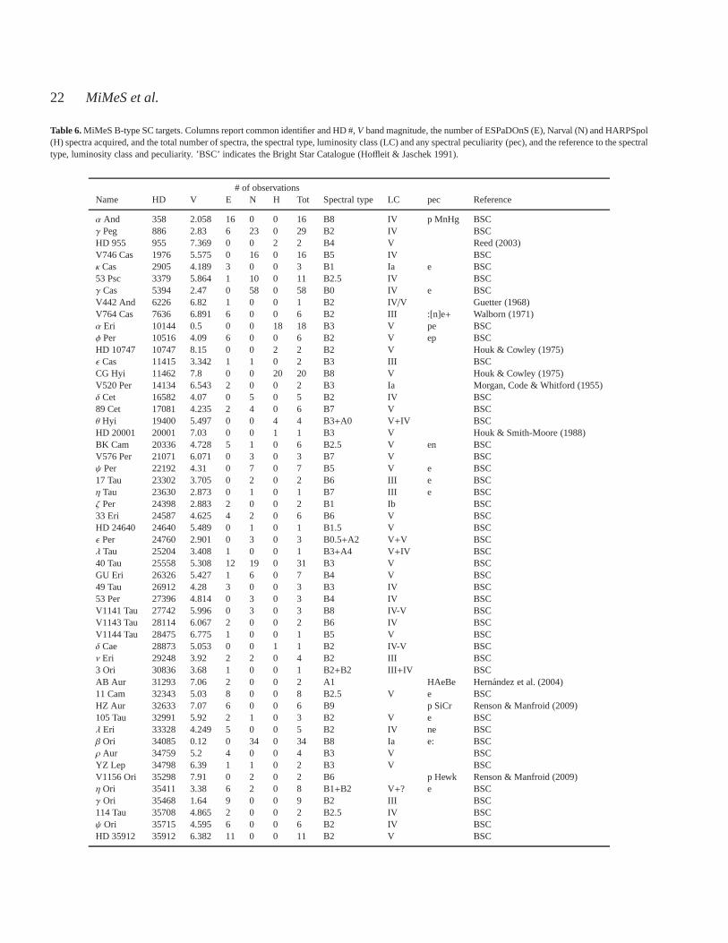
22 MiMeS et al.

Table 6. MiMeS B-type SC targets. Columns report common identifier and HD #,V band magnitude, the number of ESPaDOnS (E), Narval (N) and HARPSpol(H) spectra acquired, and the total number of spectra, the spectral type, luminosity class (LC) and any spectral peculiarity (pec), and the reference to the spectraltype, luminosity class and peculiarity. ’BSC’ indicates the Bright Star Catalogue (Hoffleit & Jaschek 1991).

# of observationsName HD V E N H Tot Spectral type LC pec Reference

α And 358 2.058 16 0 0 16 B8 IV p MnHg BSCγ Peg 886 2.83 6 23 0 29 B2 IV BSCHD 955 955 7.369 0 0 2 2 B4 V Reed (2003)V746 Cas 1976 5.575 0 16 0 16 B5 IV BSCκ Cas 2905 4.189 3 0 0 3 B1 Ia e BSC53 Psc 3379 5.864 1 10 0 11 B2.5 IV BSCγ Cas 5394 2.47 0 58 0 58 B0 IV e BSCV442 And 6226 6.82 1 0 0 1 B2 IV/V Guetter (1968)V764 Cas 7636 6.891 6 0 0 6 B2 III :[n]e+ Walborn (1971)α Eri 10144 0.5 0 0 18 18 B3 V pe BSCφ Per 10516 4.09 6 0 0 6 B2 V ep BSCHD 10747 10747 8.15 0 0 2 2 B2 V Houk & Cowley (1975)ǫ Cas 11415 3.342 1 1 0 2 B3 III BSCCG Hyi 11462 7.8 0 0 20 20 B8 V Houk & Cowley (1975)V520 Per 14134 6.543 2 0 0 2 B3 Ia Morgan, Code & Whitford (1955)δ Cet 16582 4.07 0 5 0 5 B2 IV BSC89 Cet 17081 4.235 2 4 0 6 B7 V BSCθ Hyi 19400 5.497 0 0 4 4 B3+A0 V+IV BSCHD 20001 20001 7.03 0 0 1 1 B3 V Houk & Smith-Moore (1988)BK Cam 20336 4.728 5 1 0 6 B2.5 V en BSCV576 Per 21071 6.071 0 3 0 3 B7 V BSCψ Per 22192 4.31 0 7 0 7 B5 V e BSC17 Tau 23302 3.705 0 2 0 2 B6 III e BSCη Tau 23630 2.873 0 1 0 1 B7 III e BSCζ Per 24398 2.883 2 0 0 2 B1 Ib BSC33 Eri 24587 4.625 4 2 0 6 B6 V BSCHD 24640 24640 5.489 0 1 0 1 B1.5 V BSCǫ Per 24760 2.901 0 3 0 3 B0.5+A2 V+V BSCλ Tau 25204 3.408 1 0 0 1 B3+A4 V+IV BSC40 Tau 25558 5.308 12 19 0 31 B3 V BSCGU Eri 26326 5.427 1 6 0 7 B4 V BSC49 Tau 26912 4.28 3 0 0 3 B3 IV BSC53 Per 27396 4.814 0 3 0 3 B4 IV BSCV1141 Tau 27742 5.996 0 3 0 3 B8 IV-V BSCV1143 Tau 28114 6.067 2 0 0 2 B6 IV BSCV1144 Tau 28475 6.775 1 0 0 1 B5 V BSCδ Cae 28873 5.053 0 0 1 1 B2 IV-V BSCν Eri 29248 3.92 2 2 0 4 B2 III BSC3 Ori 30836 3.68 1 0 0 1 B2+B2 III+IV BSCAB Aur 31293 7.06 2 0 0 2 A1 HAeBe Hernandez et al. (2004)11 Cam 32343 5.03 8 0 0 8 B2.5 V e BSCHZ Aur 32633 7.07 6 0 0 6 B9 p SiCr Renson & Manfroid (2009)105 Tau 32991 5.92 2 1 0 3 B2 V e BSCλ Eri 33328 4.249 5 0 0 5 B2 IV ne BSCβ Ori 34085 0.12 0 34 0 34 B8 Ia e: BSCρ Aur 34759 5.2 4 0 0 4 B3 V BSCYZ Lep 34798 6.39 1 1 0 2 B3 V BSCV1156 Ori 35298 7.91 0 2 0 2 B6 p Hewk Renson & Manfroid (2009)η Ori 35411 3.38 6 2 0 8 B1+B2 V+? e BSCγ Ori 35468 1.64 9 0 0 9 B2 III BSC114 Tau 35708 4.865 2 0 0 2 B2.5 IV BSCψ Ori 35715 4.595 6 0 0 6 B2 IV BSCHD 35912 35912 6.382 11 0 0 11 B2 V BSC

The MiMeS Survey: Introduction and Overview23

Table 6 – continuedMiMeS B-type SC targets.

# of observationsName HD V E N H Tot Spectral type LC pec Reference

HD 36629 36629 7.64 1 0 1 B2.5 IV Abt & Levato (1977)37 Ori 36822 4.398 1 0 0 1 B0 III BSCHD 36959 36959 5.67 1 0 0 1 B1 V v BSCHD 36960 36960 4.78 1 0 0 1 B0.5 V BSCV1046 Ori 37017 6.553 10 0 0 10 B1.5 V BSC41 Ori A 37020 6.73 3 0 0 3 B0.2 V Maiz Apellaniz (priv. comm.)41 Ori D 37023 6.71 4 0 0 4 B0.5 V p BSCHD 37042 37042 6.02 1 0 0 1 B0.5 V Nieva (2013)ǫ Ori A 37128 1.7 9 61 0 70 B0 Ia e BSCζ Tau 37202 3.03 0 3 0 3 B4 III pe BSCHD 37525Ab 37525 8.06 2 0 0 2 B5 Caballero, Albacete-Colombo &Lopez-Santiago (2010)α Col 37795 2.6 6 0 0 6 B7 IV e BSCHD 38120 38120 9.08 0 1 0 1 B9 e Vieira et al. (2003)κ Ori 38771 2.049 36 0 0 36 B0.5 Ia v BSCγ Col 40494 4.35 1 0 0 1 B2.5 IV BSC62 Ori 41117 4.646 1 0 0 1 B2 Ia ve BSCHD 43317 43317 6.611 0 19 0 19 B3 IV BSC7 Mon 44112 5.246 0 1 0 1 B2.5 V BSCζ CMa 44402 3 0 0 2 2 B2.5 V BSCHD 44506 44506 5.525 0 0 1 1 B1.5 V e BSCβ CMa 44743 2 1 0 0 1 B1 II-III BSCHD 45284 45284 7.37 1 0 0 1 B6 V Dworetsky, Whitelock & Carnochan (1982)10 Mon 45546 5.035 0 1 0 1 B2 V BSCβ1 Mon A 45725 4.62 2 0 0 2 B3 V e BSCV727 Mon 46005 8 1 0 0 1 B3 IV Wang et al. (2008)4 CMa 46328 4.33 25 0 0 25 B0.5 IV BSCHD 46769 46769 5.791 0 2 0 2 B8 Ib BSCV684 Mon 47755 8.43 2 0 0 2 B4 V Wang et al. (2008)HD 47934 47934 8.88 3 1 0 4 B7 V Perez, The & Westerlund (1987)HD 47961 47961 7.51 1 0 0 1 B2 V Perez, The & Westerlund (1987)HD 48055 48055 9 2 0 0 2 B3 V Turner (1976)10 CMa 48917 5.222 0 0 1 1 B2 III e BSC16 Mon 48977 5.92 1 1 0 2 B2.5 V BSCV739 Mon 49330 8.95 0 44 0 44 B1 IV nep Perez, The & Westerlund (1987)V715 Mon 49567 6.146 2 3 0 5 B3 II-III BSCκ CMa 50013 3.515 0 0 3 3 B1.5 IV ne BSCV742 Mon 50083 6.92 0 2 0 2 B2 :V :nne Morgan, Code & Whitford (1955)HD 50209 50209 8.36 0 15 0 15 B8 IV e Fremat et al. (2006)15 CMa 50707 4.806 5 0 0 5 B1 IV BSCHD 50820 50820 6.27 1 0 0 1 B3+K2 IV+II e BSCHD 51756 51756 7.18 0 1 0 1 B V Wang et al. (2008)ǫ CMa 52089 1.513 2 0 0 2 B2 II BSCGU CMa 52721 6.58 0 2 0 2 B3 V ne? Wang et al. (2008)19 Mon 52918 4.99 0 8 0 8 B1 V BSCV750 Mon 53367 7.04 2 5 0 7 B0 IV :e Morgan, Code & Whitford (1955)FN CMa 53974 5.39 2 4 0 6 B0.5 IV BSCFV CMa 54309 5.71 1 0 0 1 B2I V e BSC26 CMa 55522 5.895 1 0 0 1 B2 V BSCGY CMa 55857 6.096 0 0 2 2 B0.5 V BSCω CMa 56139 4.028 4 0 0 4 B2 IV-V e BSCOT Gem 58050 6.448 1 3 0 4 B2 V e BSCHD 58260 58260 6.734 1 0 0 1 B2 V p Garrison, Hiltner & Schild (1977)FW CMa 58343 5.2 2 0 0 2 B2.5 IV e BSCHD 58509 58509 8.57 2 0 0 2 B0 V Fitzgerald et al. (1979)

24 MiMeS et al.

Table 6 – continuedMiMeS B-type SC targets.

# of observationsName HD V E N H Tot Spectral type LC pec Reference

HD 58647 58647 6.85 0 0 1 1 B9 IV e Houk & Smith-Moore (1988)β CMi 58715 2.886 20 14 0 34 B8 V e BSCFY CMa 58978 5.56 3 0 0 3 B0 IV :pe BSCV343 Pup 60431 8.57 1 0 0 1 B4 p SiMg Renson & Manfroid (2009)PT Pup 61068 5.693 1 0 0 1 B2 III BSCHD 61555 61555 4.635 3 0 0 3 B6 V BSCHD 61556 61556 4.429 17 0 0 17 B5 IV n BSCHD 62367 62367 7.13 1 0 0 1 B6 III Jaschek et al. (1980)HD 63425 63425 6.909 8 0 0 8 B0.5 V Garrison, Hiltner & Schild (1977)b Pup 64503 4.48 0 0 1 1 B2.5 V BSCJ Pup 64760 4.234 13 0 0 13 B0.5 Ib BSCχ Car 65575 3.444 0 0 1 1 B3 IV p BSC5 Cnc 65873 5.983 1 0 0 1 B9.5 V n BSCV695 Mon 65875 6.51 2 2 0 4 B2.5 V e BSCHD 66665 66665 7.81 5 16 0 21 B0.7 IV-V Walborn (1971)HD 66765 66765 6.622 0 0 10 10 B2 V Garrison, Hiltner & Schild (1977)HD 67041 67041 7.41 0 0 1 1 B3 III/IV Houk (1978)MX Vel 67341 6.163 0 0 2 2 B3 V np BSCHD 67621 67621 6.316 0 0 8 8 B2.5 III Garrison, Hiltner & Schild(1977)V420 Pup 67698 6.53 1 0 0 1 B5 IV Abt (1985)HD 68092 68092 7.2 0 0 2 2 B3 V Garrison, Hiltner & Schild (1977)HD 68243 68243 4.2 0 0 1 1 B1 IV BSCIS Vel 68324 5.217 0 0 2 2 B1 IV e BSCHD 68395 68395 8.1 0 0 3 3 B4 V Houk (1978)HD 68451 68451 7.32 0 0 4 4 B5 II Houk (1978)HD 68657 68657 5.805 0 0 1 1 B3 V BSCHD 71072 71072 6.89 0 2 0 2 B7 IV e Buscombe (1969)HD 72067 72067 5.81 0 0 1 1 B2 V en BSCHD 74273 74273 5.878 0 0 5 5 B1.5 V BSCη Hya 74280 4.3 5 2 0 7 B3 V BSCHY Vel 74560 4.817 3 0 0 3 B3 IV BSCα Pyx 74575 3.675 3 0 0 3 B1.5 III BSCHD 75126 75126 7.08 0 0 1 1 B4 V Levato & Malaroda (1975)HD 75290 75290 8.09 0 0 2 2 B9 V Levato & Malaroda (1975)HD 75324 75324 7.12 0 0 2 2 B5 V Levato & Malaroda (1975)HD 75387 75387 6.42 0 0 1 1 B2 IV-V BSCHD 75446 75446 7.38 0 0 1 1 B6 V Levato & Malaroda (1975)HD 75657 75657 7.48 0 0 2 2 B6 III Houk (1978)HD 75724 75724 7.69 0 0 1 1 B2 IV Garrison, Hiltner & Schild (1977)HD 75758 75758 8.95 0 0 2 2 B3-5 V Houk (1978)f Vel 75821 5.094 2 0 0 2 B0 III BSCOU Vel 76534 8.02 2 0 0 2 B2/B3 Vieira et al. (2003)HD 76838 76838 7.31 0 0 1 1 B2.5 V Garrison, Hiltner & Schild (1977)HD 76868 76868 8.04 2 0 0 2 B6 e Slettebak, Wagner & Bertram (1997)IU Vel 77320 6.05 0 0 1 1 B2.5 V ne BSCIZ Vel 77475 5.541 0 0 1 1 B5 V BSCKK Vel 78616 6.786 0 0 1 1 B2 III Garrison, Hiltner & Schild (1977)E Car 78764 4.654 0 0 1 1 B2I V e BSCHD 79694 79694 5.839 0 0 1 1 B6 IV BSCHD 79791 79791 9.4 0 0 2 2 B9 V Slawson & Reed (1988)HD 80279 80279 9.45 0 0 2 2 B3 II/III Houk (1978)HD 80761 80761 7.256 0 0 2 2 B5 III Houk (1978)V335 Vel 85953 5.932 1 0 0 1 B2 III BSCEO Leo 87015 5.657 0 5 0 5 B2.5 IV BSCα Leo 87901 1.4 66 10 0 76 B7 V BSC23 Sex 89688 6.635 4 4 0 8 B2.5 IV BSCHD 89884 89884 7.131 0 2 0 2 B6 V Hill (1970)

The MiMeS Survey: Introduction and Overview25

Table 6 – continuedMiMeS B-type SC targets.

# of observationsName HD V E N H Tot Spectral type LC pec Reference

V507 Car 90966 6.429 0 0 2 2 B2/B3 III :ne Houk (1978)HD 91120 91120 5.592 0 4 0 4 B9 V ne BSCρ Leo 91316 3.87 2 5 0 7 B1 Ib BSCHD 91969 91969 6.51 0 0 1 1 B0 Iab e Evans et al. (2005)V518 Car 92938 4.82 0 0 1 1 B4 V BSCθ Car 93030 2.78 0 0 3 3 B0 V p BSCHD 93194 93194 4.786 0 0 1 1 B5 V n BSCHD 93607 93607 4.85 0 0 1 1 B3 IV BSCHD 93714 93714 6.545 0 0 1 1 B2 IV/V n Abt & Morgan (1972)HD 94097 94097 7.2 0 0 1 1 B3 V Houk & Cowley (1975)π Cen 98718 3.9 0 0 4 4 B5 V n BSCHD 98922 98922 6.76 1 0 1 2 B9 e Vieira et al. (2003)KR Mus 100546 6.7 0 0 1 1 B9 V ne Houk & Cowley (1975)90 Leo 100600 5.94 4 0 0 4 B4 V BSCHD 101391 101391 6.334 0 4 0 4 B9 p HgMn: BSCHD 103079 103079 4.929 0 0 1 1 B4 V BSC31 Crt 104337 5.263 6 3 0 9 B1.5 V BSCθ2 Cru 104841 4.718 0 0 1 1 B2 IV BSCV863 Cen 105382 4.448 0 0 3 3 B6 III e BSCδ Cen 105435 2.561 0 0 3 3 B2 IV ne BSCρ Cen 105937 3.951 0 0 1 1 B3 V BSCδ Cru 106490 2.775 0 0 3 3 B2 IV BSCζ Cru 106983 4.05 0 0 2 2 B2.5 V BSCα1 Cru 108248 1.4 0 0 4 4 B0.5 IV BSCG Cen 108257 4.805 0 0 2 2 B3 V n BSCσ Cen 108483 3.897 0 0 1 1 B2 V BSCγ Mus 109026 3.83 0 0 9 9 B5 V BSCκ Dra 109387 3.881 9 18 0 27 B6 III pe BSCα Mus 109668 2.677 0 0 1 1 B2 IV-V BSC39 Cru 110335 4.94 0 0 1 1 B6 IV e BSCBZ Cru 110432 5.316 0 0 2 2 B2 pe BSCβ Mus 110879 3.07 0 0 4 4 B2.5 V BSCHD 110956 110956 4.612 0 0 1 1 B3 V BSCβ Cru 111123 1.297 0 0 6 6 B0.5 III BSCµ2 Cru 112091 5.113 0 0 1 1 B5 V ne BSCHD 112092 112092 3.988 0 0 1 1 B2 IV-V BSCf Cen 113703 4.694 0 0 2 2 B5 V BSCHD 113791 113791 4.264 0 0 12 12 B1.5 V BSC15 CVn 114376 6.28 0 2 0 2 B7 III BSCV958 Cen 114981 7.12 1 0 0 1 B5 V e Vieira et al. (2003)HD 115846 115846 7.023 0 0 2 2 B3 IV Houk & Cowley (1975)V790 Cen 116072 6.198 0 0 2 2 B2.5 V n BSCJ Cen 116087 4.505 0 0 2 2 B3 V BSCα Vir 116658 1.04 0 8 0 8 B1+B2 III-IV +V BSCǫ Cen 118716 2.265 0 0 8 8 B1 III BSCν Cen 120307 3.39 0 0 2 2 B2I V BSCη UMa 120315 1.852 0 8 0 8 B3 V BSCµ Cen 120324 3.456 6 0 0 6 B2 IV-V e BSCHD 120640 120640 5.75 0 0 1 1 B2 V p BSCφ Cen 121743 3.806 0 0 2 2 B2I V BSCHD 121790 121790 3.842 0 0 1 1 B2 IV-V BSCβ Cen 122451 0.6 0 0 63 63 B1 III BSCχ Cen 122980 4.343 0 0 1 1 B2 V BSCτ1 Lup 126341 4.546 0 0 1 1 B2 IV BSCσ Lup 127381 4.416 17 0 0 17 B2 III BSCρ Lup 128345 4.034 0 0 2 2 B5 V BSC

26 MiMeS et al.

Table 6 – continuedMiMeS B-type SC targets.

# of observationsName HD V E N H Tot Spectral type LC pec Reference

α Lup 129056 2.276 0 0 1 1 B1.5 III BSCV836 Cen 129929 8.05 1 0 0 1 B3 V Hill (1970)o Lup 130807 4.313 0 0 12 12 B5 IV BSCβ Lup 132058 2.665 0 0 6 6 B2 III BSCκ Cen 132200 3.13 0 0 2 2 B2 IV BSCHD 132955 132955 5.427 0 0 1 1 B3 V BSCπ Lup A 133242 4.59 0 0 2 2 B5 V BSCHD 133518 133518 6.396 0 0 3 3 B2 V p HeStr Garrison, Hiltner & Schild (1977)λ Lup 133955 4.07 0 0 2 2 B3 V BSCe Lup 134687 4.807 0 0 1 1 B3 IV BSCδ Lup 136298 3.203 0 0 6 6 B1.5I V BSCǫ Lup 136504 3.367 22 0 0 22 B2 IV-V BSCHD 137432 137432 5.442 0 0 1 1 B4 V p BSCFK Boo 138003 7.84 0 3 0 3 B8 p Si Grenier et al. (1999)θ CrB 138749 4.153 0 6 0 6 B6 V nne BSCIU Lib 138764 5.147 1 0 0 1 B6 IV BSCτ Lib 139365 3.644 0 0 1 1 B2.5 V BSC4 Lup 140008 4.717 0 0 1 1 B5 V BSC25 Ser 140873 5.39 1 8 0 9 B8 III BSCV1040 Sco 142184 5.4 27 0 0 27 B2.5 V ne BSCρ Sco 142669 3.864 0 0 1 1 B2 IV-V BSCHD 142883 142883 5.841 0 0 1 1 B3 V BSCV913 Sco 142990 5.44 2 0 0 2 B5 IV BSCπ Sco 143018 2.89 0 0 1 1 B1+B2 V BSCδ Sco 143275 2.291 11 0 0 11 B0.3 IV BSCβ Sco A 144217 2.62 11 0 0 11 B1 V BSCβ Sco C 144218 4.89 0 0 1 1 B2 V BSCω Sco 144470 3.946 0 0 1 1 B1 V BSCφ Her 145389 4.232 0 5 0 5 B9 p:Mn: BSCσ Sco 147165 2.912 3 0 0 3 B2+O9.5 III+V BSCτ Her 147394 3.9 0 4 0 4 B5 IV BSCρ Oph D 147888 6.779 0 0 2 2 B3 V Abt (1986)ρ Oph C 147932 7.27 0 0 4 4 B7 V Abt (1986)χ Oph 148184 4.42 0 4 0 4 B2 IV :pe BSCHD 149277 149277 8.41 1 0 0 1 B2 IV n Garrison, Hiltner & Schild (1977)HD 150898 150898 5.572 0 0 1 1 B0.5 Ia BSCHD 151985 151985 3.544 0 0 1 1 B2 IV BSCHD 152234 152234 5.43 1 0 0 1 B0.5 Ia BSCV1070 Sco 152635 7.66 1 0 0 1 B7 II Houk (1982)HD 153716 153716 5.727 0 0 1 1 B5 IV BSCk Sco 154090 4.861 0 0 1 1 B1 Ia e BSCHD 154664 154664 8.73 0 0 2 2 B1 IV Garrison, Hiltner & Schild (1977)HD 155217 155217 8.66 0 0 2 2 B1.5 III n Garrison, Hiltner & Schild (1977)HD 155273 155273 8.92 0 0 2 2 B3 IV Houk (1982)HD 155320 155320 8.37 0 0 2 2 B1 III Garrison, Hiltner & Schild (1977)HD 155450 155450 6.001 0 0 1 1 B 1II BSCHD 155506 155506 7.75 0 0 1 1 B1.5 V Garrison, Hiltner & Schild (1977)HD 155754 155754 7.96 0 0 1 1 B1 IV Garrison, Hiltner & Schild (1977)HD 155888 155888 8.68 0 0 2 2 B4 V Houk (1982)HD 156004 156004 7.82 0 0 2 2 B1 IV Garrison, Hiltner & Schild (1977)HD 156256 156256 8.28 0 0 2 2 B2 V n Garrison, Hiltner & Schild (1977)HD 156321 156321 8.16 0 0 2 2 B1.5 III Garrison, Hiltner & Schild (1977)HD 156324 156324 8.76 0 0 3 3 B2 V Roslund (1966)HD 156424 156424 8.9 0 0 3 3 B2 V Roslund (1966)68 Her 156633 4.8 9 0 0 9 B1.5+B5 V+III p BSCλ Sco 158926 1.62 0 0 19 19 B2 IV BSCV994 Sco 160124 7.16 1 0 0 1 B3 IV-V Houk (1982)

The MiMeS Survey: Introduction and Overview27

Table 6 – continuedMiMeS B-type SC targets.

# of observationsName HD V E N H Tot Spectral type LC pec Reference

κ Sco 160578 2.375 0 0 2 2 B1.5 III BSCι Her 160762 3.8 0 3 0 3 B3 IV BSCV1092 Sco 163254 6.74 3 0 0 3 B2 V SB2 Garrison, Hiltner & Schild(1977)66 Oph 164284 4.784 24 32 0 56 B2 V e BSCHD 164402 164402 5.749 2 0 0 2 B0 Ib BSCHD 164865 164865 7.74 0 0 2 2 B9 Ia Garrison, Hiltner & Schild (1977)HD 164906 164906 7.45 0 0 1 1 B1 IV :pe Morgan, Code & Whitford (1955)HD 164933 164933 8.7 0 0 2 2 B0.5 V Garrison, Hiltner & Schild (1977)HD 167756 167756 6.286 1 0 0 1 B0.5 Ia BSCHD 168957 168957 6.983 1 0 0 1 B3 V Guetter (1968)HD 169142 169142 8.16 3 0 0 3 A9 HAeBe Vieira et al. (2003)α Tel 169467 3.477 1 0 8 9 B3 IV BSCHD 169820 169820 6.365 1 4 0 5 B9 V BSCQT Ser 170783 7.73 0 10 0 10 B5 HAeBe Neubauer (1943)λ Pav 173948 4.207 0 0 2 2 B2 II-III e BSCCX Dra 174237 5.9 1 0 0 1 B2.5 V e BSCHD 174571 174571 8.89 0 2 0 2 B2.5 V :[n]e Walborn (1971)σ Sgr 175191 2.058 0 0 8 8 B2.5 V BSC64 Ser 175869 5.563 0 18 0 18 B9 III ep:Hg: BSCHD 176386 176386 7.3 3 0 0 3 B9 V Torres et al. (2006)V545 Lyr 176582 6.404 0 44 0 44 B5 IV BSCV4024 Sgr 178175 5.57 1 0 0 1 B2 V e BSCV338 Sge 179588 6.69 1 0 0 1 B9 IV BSCV1449 Aql 180642 8.29 11 6 0 17 B1.5 II-III Walborn (1971)2 Vul 180968 5.477 0 5 0 5 B0.5 IV BSCHD 181231 181231 8.58 0 18 0 18 B5 IV eV4199 Sgr 181558 6.244 0 2 0 2 B5 V BSCHD 182180 182180 6.023 4 0 0 4 B2 V n BSC3 Vul 182255 5.19 1 4 0 5 B6 III BSC2 Cyg 182568 4.976 1 0 0 1 B3 IV BSCV4372 Sgr 183133 6.777 1 0 0 1 B4 V Buscombe (1969)HD 186205 186205 8.54 1 0 0 1 B2 V p HeStr Levato & Malaroda (1975)V1339 Aql 187567 6.484 1 0 0 1 B2.5 IV e BSC12 Vul 187811 4.893 3 0 0 3 B2.5 V e BSC25 Cyg 189687 5.139 3 0 0 3 B3I V e BSCV2100 Cyg 189775 6.114 2 0 0 2 B5 III BSCV1473 Aql 191295 7.16 0 3 0 3 B7 III Crampton & Byl (1971)28 Cyg 191610 4.929 6 0 0 6 B2.5 V e BSCQR Vul 192685 4.759 2 12 0 14 B3 V BSC34 Cyg 193237 4.795 0 3 0 3 B2 pe BSCλ Cyg 198183 4.75 0 5 0 5 B5 V e BSC55 Cyg 198478 4.858 1 0 0 1 B3 Ia e BSCBW Vul 199140 6.54 1 0 0 1 B2 III v BSCυ Cyg 202904 4.43 0 28 0 28 B2 V ne BSC6 Cep 203467 5.185 5 2 0 7 B3 IV e BSCHD 203532 203532 6.358 0 0 2 2 B3 IV BSCSY Equ 203664 8.53 0 3 0 3 B0.5 III (n) Walborn (1971)V429 Cep 205196 7.439 1 0 0 1 B0 Ib Garrison & Kormendy (1976)HD 205329 205329 8.07 1 0 0 1 B1.5 V Garrison & Kormendy (1976)ǫ Cap 205637 4.5 5 0 2 7 B2.5 V pe BSCHD 205794 205794 8.43 1 0 0 1 B0.5 V Garrison & Kormendy (1976)DK Oct 205879 7.62 0 0 4 4 B8 V Houk & Cowley (1975)HD 205948 205948 8.6 1 0 0 1 B2 IV Garrison & Kormendy (1976)HD 206081 206081 8.24 1 0 0 1 B1: V n SB2 Garrison & Kormendy (1976)9 Cep 206165 4.788 7 0 0 7 B2 Ib BSC

28 MiMeS et al.

Table 6 – continuedMiMeS B-type SC targets.

# of observationsName HD V E N H Tot Spectral type LC pec Reference

HD 206540 206540 6.052 1 2 0 3 B5 IV BSC81 Cyg 207330 4.18 0 2 0 2 B3 III BSCHD 208213 208213 8.54 0 0 2 2 B3 IV Houk (1982)o Aqr 209409 4.7 0 2 0 2 B7 IV e BSC35 Aqr 210191 5.791 0 0 1 1 B2.5 IV BSC31 Peg 212076 4.81 24 0 0 24 B2 IV-V e BSCπ Aqr 212571 4.794 8 0 0 8 B1 V e BSC4 Lac 212593 4.599 11 0 0 11 B9 Iab BSC6 Lac 213420 4.518 0 3 0 3 B2 IV BSCǫ PsA 214748 4.18 0 0 3 3 B8 V e BSC12 Lac 214993 5.228 0 3 0 3 B2 III BSC14 Lac 216200 5.928 0 3 0 3 B3 IV :e BSCIL Cep 216629 9.31 1 1 0 2 B2 IV-V ne Garrison (1970)16 Lac 216916 5.584 1 3 0 4 B2 IV BSCKZ Cep 217035 7.74 0 3 0 3 B0 IV :(n) Walborn (1971)EW Lac 217050 5.42 2 1 0 3 B4 III ep BSCo And 217675 3.633 0 1 0 1 B6+A2 III pe+p BSCβ Psc 217891 4.486 21 0 0 21 B6 V e BSC1 Cas 218376 4.84 5 25 0 30 B0.5 IV BSCHD 220787 220787 8.29 0 0 1 1 B3 III Hill (1970)V352 Peg 221218 7.12 1 0 0 1 B8-9 III Grenier et al. (1999)β Scl 221507 4.37 0 0 2 2 B9.5 IV pHgMnEu BSCV394 And 222555 7.42 0 3 0 3 B9σ Phe 223145 5.161 0 0 2 2 B3 V BSCV373 Cas 224151 6.045 4 0 0 4 B0.5 II v BSCǫ Tuc 224686 4.49 0 0 3 3 B9 IV BSCζ Scl 224990 5.023 0 0 3 3 B4 III BSCV432 Cep 239712 8.53 1 0 0 1 B3: IV nep Garrison & Kormendy (1976)HD 239729 239729 8.36 1 0 0 1 B0 V Walborn (1971)HD 249879 249879 10.62 0 1 0 1 B8? e HAeBe Vieira et al. (2003)V1307 Ori 250550 9.593 0 1 0 1 B9 e Hernandez et al. (2004)HD 259012 259012 9.27 3 0 0 3 B1 V n Morgan et al. (1965)HD 259105 259105 9.419 1 0 0 1 B1.5 V Morgan et al. (1965)BD+04 1299 259135 8.542 6 2 0 8 B0.5 V Morgan et al. (1965)HD 259172 259172 10.712 1 0 0 1 B2 V Massey, Johnson & Degioia-Eastwood (1995)V700 Mon 259431 8.81 0 3 0 3 B6 e Hernandez et al. (2004)HD 261657 261657 10.88 1 0 0 1 B9 V HAeBe Perez, The & Westerlund(1987)HD 261902 261902 10.2 1 0 0 1 B8 HAeBe Perez, The & Westerlund (1987)HD 261937 261937 10.36 1 0 0 1 B8 HAeBeHD 261939 261939 10.96 1 0 0 1 B9 V Paunzen et al. (2001)HD 261940 261940 10 1 0 0 1 B8 V HAeBe Paunzen et al. (2001)HD 261969 261969 9.95 1 0 0 1 B9 IV HAeBe Paunzen et al. (2001)HD 262013 262013 9.34 1 0 0 1 B8 HAeBe Perez, The & Westerlund (1987)HD 290409 290409 9.96 0 1 0 1 B9 e, HAeBe Vieira et al. (2003)HD 290500 290500 11.04 0 2 0 2 B8 HAeBe Vieira et al. (2003)HD 290770 290770 9.3 0 1 0 1 B9 e, HAeBe Vieira et al. (2003)HD 308096 308096 9.53 0 0 2 2 B1 II: SB2? Garrison, Hiltner & Schild (1977)HD 315021 315021 8.59 0 0 2 2 B2 IV n Hiltner, Morgan & Neff (1965)HD 315031 315031 8.3 0 0 1 1 B2 IV n Hiltner, Morgan & Neff (1965)HD 315033 315033 8.9 0 0 2 2 B2 V p Hiltner, Morgan & Neff (1965)BD-13 4912 10.02 1 0 0 1 B2.5 I Hillenbrand et al. (1993)BD-13 4933 10.628 1 0 0 1 B0.5 V e Hillenbrand et al. (1993)BD-13 4935 10.99 1 0 0 1 B3 V Hillenbrand et al. (1993)BD-13 4937 10.78 26 5 0 31 B1.5 V Hillenbrand et al. (1993)BD+04 1295p 10.641 3 0 0 3 B2.5 V Massey, Johnson & Degioia-Eastwood (1995)

The MiMeS Survey: Introduction and Overview29

Table 6 – continuedMiMeS B-type SC targets.

# of observationsName HD V E N H Tot Spectral type LC pec Reference

BD+04 1299s 9.735 0 1 0 1 B1 III Massey, Johnson & Degioia-Eastwood (1995)BD+05 1281B 10.73 1 0 0 1 B1.5 V Massey, Johnson & Degioia-Eastwood (1995)BD+05 1283E 11.813 1 0 0 1 B5 Iab Morgan et al. (1965)BD+09 1331B 10.79 1 0 0 1 B1 V Paunzen et al. (2001)BD+10 1222 9.88 1 0 0 1 B8 V Perez, The & Westerlund (1987)BD+41 3731 9.84 1 1 0 2 B2 Finkenzeller (1985)EU Ser 13.0 1 0 0 1 B9 III HAeBe Evans et al. (2005)NGC 2244 119 12.353 1 0 0 1 B6 VNGC 2244 125 12.032 1 0 0 1 B4 VNGC 2244 130 11.662 1 0 0 1 B2.5 V Wang et al. (2008)NGC 2244 172 11.222 1 0 0 1 B2.5 V Morgan et al. (1965)NGC 2244 190 11.255 1 0 0 1 B2.5 V n Morgan et al. (1965)NGC 2244 194 12.006 1 0 0 1 B6 V ne Morgan et al. (1965)NGC 2244 195 12.151 1 0 0 1 B7 VNGC 2244 274 11.43 1 0 0 1 B2.5 V Massey, Johnson & Degioia-Eastwood (1995)NGC 2244 74 11.41 1 0 0 1 B7 V e Li et al. (2002)NGC 2244 80 9.39 1 0 0 1 B0.5 V Johnson (1962)NGC 2264 181 10.03 1 0 0 1 B8 V n Paunzen et al. (2001)NGC 6611 080 13.593 8 0 0 8 B2 V HAeBe Hillenbrand et al. (1993)NGC 6611 090 11.73 1 0 0 1 B5 V Dufton et al. (2006)NGC 6611 207 12.05 1 0 0 1 B1 V e Wolff et al. (2007)NGC 6611 235 11.127 3 0 0 3 B e Dufton et al. (2006)NGC 6611 254 10.8 1 0 0 1 B1 V Wolff et al. (2007)NGC 6611 289 12.57 1 0 0 1 B3 V Dufton et al. (2006)NGC 6611 306 12.72 4 0 0 4 B1.5 V e Hillenbrand et al. (1993)NGC 6611 489 11.42 1 0 0 1 B8 III Dufton et al. (2006)NGC 6611 500 11.23 1 0 0 1 B5 e Evans et al. (2005)NGC 6611 520 11.63 1 0 0 1 B5 III n Dufton et al. (2006)NGC 6611 536 11.42 1 0 0 1 B1.5 V Wolff et al. (2007)TY CrA 9.42 2 0 0 2 B9 e Meyer & Wilking (2009)V1578 Cyg 10.16 1 0 0 1 B9 e Hernandez et al. (2004)V361 Cep 10.17 1 1 0 2 B4 e Hernandez et al. (2004)V594 Cas 10.64 2 0 0 2 B8 eq Finkenzeller (1985)V628 Cas 11.582 1 0 0 1 B0 eq Manoj et al. (2006)V699 Mon 10.7 0 2 0 2 B6 e Hernandez et al. (2004)VV Ser 11.82 1 0 0 1 B6 e Hernandez et al. (2004)V1230 Ori 9.736 9 0 0 9 B0 V p Johnson (1965)

30 MiMeS et al.

Affiliations1Department of Physics, Royal Military College of Canada, POBox 17000, Stn Forces, Kingston, Ontario K7K 7B4, Canada2LESIA, Observatoire de Paris, PSL Research University, CNRS, Sorbonne Universites, UPMC, Univ. Paris 6, Univ. Paris Diderot, Sorbonne Paris Cite, 5place Jules Janssen, 92195, Meudon, France3UJF-Grenoble 1/CNRS-INSU, Institut de Planetologie et d’Astrophysique de Grenoble (IPAG) UMR 5274, 38041, Grenoble, France4CNRS-IPAG, F-38000, Grenoble, France5European Organisation for Astronomical Research in the Southern Hemisphere, Karl-Schwarzschild-Str. 2, D-85748 Garching, Germany6Dept. of Physics & Space Sciences, Florida Institute of Technology, Melbourne, FL, USA7Herzberg Astronomy and Astrophysics Program, National Research Council of Canada, 5071 West Saanich Road, Victoria, BC V9E 2E7, Canada8Swarthmore College, Department of Physics and Astronomy, Swarthmore, PA 19081, USA9Anton Pannekoek Institute for Astronomy, University of Amsterdam, Science Park 904, 1098 XH Amsterdam, The Netherlands10Department of Physics and Astronomy, Uppsala University, Box 516, 75120, Uppsala, Sweden11Physics & Astronomy Department, The University of Western Ontario, London, Ontario, N6A 3K7, Canada12Armagh Observatory, College Hill, Armagh BT61 9DG, UK13Canada-France-Hawaii Telescope Corporation, 65-1238 Mamalahoa Hwy Kamuela HI 96743, USA14LUPM, CNRS & Universite de Montpellier, Place EugEne Bataillon, F-34095, Montpellier Cedex 05, France15Laboratoire AIM Paris-Saclay, CEA/DSM, CNRS, Universite Paris Diderot, IRFU/SAp Centre de Saclay, F-91191 Gif-sur-Yvette, France16University of Delaware, Bartol Research Institute, Newark, DE 19716, USA17European Organisation for Astronomical Research in the Southern Hemisphere, Casilla 19001, Santiago, Chile18Department of Physics, Engineering Physics and Astronomy,Queen’s University, 99 University Avenue, Kingston, ON K7L3N6, Canada19Institut fur Astronomie und Astrophysik der UniversitatMunchen, Scheinerstr. 1, D-81679 Munchen, Germany20Department of Astronomy, University of Wisconsin Madison,2535 Sterling Hall, 475 North Charter St, Madison, WI 53706,USA21Department of Physics, Penn State Worthington Scranton, 120 Ridge View Drive, Dunmore, PA 18512, USA22Aix Marseille Universite, CNRS, LAM (Laboratoire d’Astrophysique de Marseille) UMR 7326, 13388, Marseille, France23Argelander Institut fur Astronomie, Auf dem Hugel 71, 53121 Bonn, Germany24Institut d?Astrophysique et de Geophysique, Universitede Liege, Quartier Agora, 19c, Allee du 6 Aout, B5c, B-4000 Sart Tilman, Belgium25Instituto de Astronomia, Geofısica e Ciencias Atmosfericas, Universidade de Sao Paulo, Rua do Matao 1226, CidadeUniversitaria, Sao Paulo, SP05508-900, Brazil26Space Telescope Science Institute, 3700 San Martin Drive, Baltimore, MD 21218, USA27Universidade Federal do Rio de Janeiro, Observatorio do Valongo, Ladeira Pedro AntUnio, 43, CEP 20.080-090, Rio de Janeiro, Brazil28Departement de Physique and Centre de Recherche en Astrophysique du QuEbec, Universite de Montreal, C.P. 6128, Succ. C-V, Montreal, QC, H3C 3J7,Canada29Universite de Toulouse; UPS-OMP; IRAP; Toulouse, France30CNRS-IRAP; 14, avenue Edouard Belin, 31400 Toulouse, France31Max Planck Insitut fur Extraterrestrische Physik, Giessenbachstrasse 1, 85748 Garching, Germany32Departamento de Fısica, Universidad de La Serena, Av. JuanCisternas 1200 Norte, La Serena, Chile33Observatoire de Paris, PSL Research University, 61 avenue de l’Observatoire, 75014 Paris, France34Department of Mathematics, Mathematical Sciences Institute, The Australian National University, ACT 0200 Australia35Kiepenheuer-Institut fur Sonnenphysik, Schoneckstr. 6, D-79104 Freiburg, Germany36Institute for Astronomy, University of Hawaii, 2680 Woodlawn Drive, Honolulu, HI, 96822, USA37Applied Research Labs, University of Hawaii, 2800 WoodlawnDrive, Honolulu, HI, 96822, USA38Department of Physics & Astronomy, University College London, Gower St, London WC1E 6BT, UK39Department of Physics and Astronomy, East Tennessee State University, Johnson City, TN 37614, USA40Department of Astrophysics, University of Vienna, Tuerkenschanzstrasse 17, 1180 Vienna, Austria41Special Astrophysical Observatory, Russian Academy of Sciences, Nizhny Arkhyz, Russia 36916742Centro de Astrobiologıa, CSIC-INTA, Ctra. Torrejon a Ajalvir km.4, 28850 Madrid, Spain43Instituut voor Sterrenkunde, KU Leuven, Celestijnenlaan 200D, 3001 Leuven, Belgium