the mexican livestock, meat, and …afcerc.tamu.edu/publications/publication-pdfs/im 3 96...
TRANSCRIPT
THE MEXICAN LIVESTOCK, MEAT, AND FEEDGRAIN INDUSTRIES: A DYNAMIC
ANALYSIS OF U.S.-MEXICO ECONOMIC INTEGRATION
José García-Vega and Gary W. Williams*
TAMRC International MarketResearch Report No. IM-3-96
August 1996
*Assistant Professor, Texas A&M University - Kingsville and Professor and TAMRC Director,Department of Agricultural Economics, Texas A&M University, respectively.

The Mexican Livestock, Meat, and Feed Grain Industries: A Dynamic Analysis of U.S. -Mexico Economic Integration
Texas Agricultural Market Research Center (TAMRC) International Market Research ReportNo. IM-3-96, August 1996 by José García-Vega and Gary W. Williams.
ABSTRACT: This study provides a comprehensive, consistent assessment of the potential impactsof freer U.S.-Mexico agricultural trade on the Mexican livestock, meat, and feedgrain industries.Background information of the Mexican livestock, meat, and feedgrain industries is provided. Atheoretical model of U.S.-Mexico trade in livestock, meat, and feedgrains is developed which isvalidated through historical simulation and sensitivity analysis. The model is used to simulate themarket effects of the unilateral liberalization of Mexican livestock, meat, and feedgrain trade over10-year period prior to the implementation of NAFTA. In general, the analysis indicated that theMexican policy shift to more open markets substantially impacted Mexican livestock, meat, andfeedgrain trade. The results also clearly indicated that the effects of liberalizing Mexican livestock,meat, and feedgrain trade were highly dependent on the level and direction of change in per capitaincome during the period of liberalization.
The Texas Agricultural Market Research Center (TAMRC) has been providing timely, unique,and professional research on a wide range of issues relating to agricultural markets andcommodities of importance to Texas and the nation for more than twenty-five years. TAMRC isa market research service of the Texas Agricultural Experiment Station and the Texas AgriculturalExtension Service. The main TAMRC objective is to conduct research leading to expanded andmore efficient markets for Texas and U.S. agricultural products. Major TAMRC research divisionsinclude International Market Research, Consumer and Product Market Research, CommodityMarket Research, and Contemporary Market Issues Research.
The Mexican Livestock, Meat, Feed Grain Industries: A Dynamic Analysis of U.S. - MexicoEconomic Integration
Executive Summary
This study provides a comprehensive, consistent assessment of the potential impacts of freer U.S.-Mexicoagricultural trade on the Mexican livestock, meat, and feedgrain industries. As background to thedevelopment of a theoretical model to analyze that trade, the characteristics of the Mexican livestock, meat,and feedgrain industries are first considered. After presenting the underlying assumptions of the model, theMexican livestock, meat, and feedgrain supply and demand relationships are discussed.
Three demand model formulations (LA/AIDS, ROTTERDAM, and single equation) are discussed for theMexican meat sector. Gross complementarity among meats is found in the LA/AIDS and the ROTTERDAMwhich prevents the use of these demand specifications. The single equation meat demand formulation isintegrated to the supply system and the parameters of the Mexican livestock, meat, and feedgrain model areestimated. The model is then validated through historical simulation and sensitivity analysis. Summarystatistics show good performance and high stability of the estimated model.
The fully integrated supply and demand model is used to simulate the effects of Mexico's trade liberalizationon the Mexican livestock, meat, and feedgrain sectors under several scenarios. Liberalization of Mexicanmarkets benefits both the livestock and feedgrain sectors in Mexico because the resulting increased demandfor livestock generated an increase in demand for feed that more than offset the negative effects generatedby increasing feed imports.
The Mexican meat processing industry also benefits from Mexican market liberalization. Even though thesimulation results indicate that meat production is lower on average after the liberalization of trade, totalrevenues actually increase because the inelastic nature of meat demand in Mexico results in a much largerpercentage increase in retail prices of meat.
Changes in real per capita income in Mexico are an important factor in determining the likely consequencesof trade liberalization on Mexican meat imports. If real per capita income in Mexico had been only onestandard deviation lower than was actually the case during the 1986 to 1991 period of unilateral liberalization,the model simulation results indicate that Mexican meat demand would have dropped enough to eliminatemeat imports altogether, possibly even creating excess Mexican supplies of meat for export.

iv
TABLE OF CONTENTS
Page
THE MEXICAN LIVESTOCK, MEAT, AND FEEDGRAIN INDUSTRIES: A DYNAMICANALYSIS OF U.S.-MEXICO ECONOMIC INTEGRATION . . . . . . . . . . . . . . . . . . . . . . . . . . . . . . . . . . . . . . . . 1
Literature Review . . . . . . . . . . . . . . . . . . . . . . . . . . . . . . . . . . . . . . . . . . . . . . . . . . . . . . . . . . . . . . . . . . . . . 2Studies of the Effects of a NAFTA on Agricultural Markets . . . . . . . . . . . . . . . . . . . . . . . . . . . . . 2Studies of the Mexican Livestock, Meat, and Feedgrain Industries . . . . . . . . . . . . . . . . . . . . . . . 2Studies That Model Livestock and Feed Markets . . . . . . . . . . . . . . . . . . . . . . . . . . . . . . . . . . . . . 3
Objectives . . . . . . . . . . . . . . . . . . . . . . . . . . . . . . . . . . . . . . . . . . . . . . . . . . . . . . . . . . . . . . . . . . . . . . . . . . 4
THE MEXICAN LIVESTOCK, MEAT, AND FEED SECTORS . . . . . . . . . . . . . . . . . . . . . . . . . . . . . . . . . . . . . . . 6The Mexican Livestock and Meat Industry . . . . . . . . . . . . . . . . . . . . . . . . . . . . . . . . . . . . . . . . . . . . . . . . . 6The Mexican Cattle and Beef Industry . . . . . . . . . . . . . . . . . . . . . . . . . . . . . . . . . . . . . . . . . . . . . . . . . . . . 7The Mexican Hog and Pork Industry . . . . . . . . . . . . . . . . . . . . . . . . . . . . . . . . . . . . . . . . . . . . . . . . . . . . . . 8The Mexican Chicken Industry . . . . . . . . . . . . . . . . . . . . . . . . . . . . . . . . . . . . . . . . . . . . . . . . . . . . . . . . . . 8The Mexican Feed Industry . . . . . . . . . . . . . . . . . . . . . . . . . . . . . . . . . . . . . . . . . . . . . . . . . . . . . . . . . . . . . 9
Mexican Sorghum Supply and Demand . . . . . . . . . . . . . . . . . . . . . . . . . . . . . . . . . . . . . . . . . . . . 9Mexican Soybeans and Soymeal Supply and Demand . . . . . . . . . . . . . . . . . . . . . . . . . . . . . . . . . 9Mexican Corn Supply and Demand . . . . . . . . . . . . . . . . . . . . . . . . . . . . . . . . . . . . . . . . . . . . . . . . 9
Mexican Agricultural Policy . . . . . . . . . . . . . . . . . . . . . . . . . . . . . . . . . . . . . . . . . . . . . . . . . . . . . . . . . . . . 9NAFTA . . . . . . . . . . . . . . . . . . . . . . . . . . . . . . . . . . . . . . . . . . . . . . . . . . . . . . . . . . . . . . . . . . . . 11
Summary . . . . . . . . . . . . . . . . . . . . . . . . . . . . . . . . . . . . . . . . . . . . . . . . . . . . . . . . . . . . . . . . . . . . . . . . . . 11
CONCEPTUAL MODEL OF THE MEXICAN LIVESTOCK, MEAT, AND FEEDGRAIN SECTORS . . . . . . . 26Underlying Assumptions of the Mexican Livestock, Meat, and Feedgrain Model . . . . . . . . . . . . . . . . . . 26Conceptual Framework for Livestock . . . . . . . . . . . . . . . . . . . . . . . . . . . . . . . . . . . . . . . . . . . . . . . . . . . . 26Conceptual Framework for Meat . . . . . . . . . . . . . . . . . . . . . . . . . . . . . . . . . . . . . . . . . . . . . . . . . . . . . . . . 28Conceptual Framework for Feedgrains . . . . . . . . . . . . . . . . . . . . . . . . . . . . . . . . . . . . . . . . . . . . . . . . . . . 28The Mexican Livestock and Meat Supply Model . . . . . . . . . . . . . . . . . . . . . . . . . . . . . . . . . . . . . . . . . . . 29The Mexican Feed Supply and Demand Model . . . . . . . . . . . . . . . . . . . . . . . . . . . . . . . . . . . . . . . . . . . . . 31The Mexican Meat Demand Model . . . . . . . . . . . . . . . . . . . . . . . . . . . . . . . . . . . . . . . . . . . . . . . . . . . . . . 32
The Almost Ideal Demand System (AIDS) . . . . . . . . . . . . . . . . . . . . . . . . . . . . . . . . . . . . . . . . . 32The Rotterdam Model . . . . . . . . . . . . . . . . . . . . . . . . . . . . . . . . . . . . . . . . . . . . . . . . . . . . . . . . . 33The Single Equation Model . . . . . . . . . . . . . . . . . . . . . . . . . . . . . . . . . . . . . . . . . . . . . . . . . . . . . 34
Linkages Between Supply and Demand . . . . . . . . . . . . . . . . . . . . . . . . . . . . . . . . . . . . . . . . . . . . . . . . . . . 34Summary . . . . . . . . . . . . . . . . . . . . . . . . . . . . . . . . . . . . . . . . . . . . . . . . . . . . . . . . . . . . . . . . . . . . . . . . . . 35
EMPIRICAL ANALYSIS . . . . . . . . . . . . . . . . . . . . . . . . . . . . . . . . . . . . . . . . . . . . . . . . . . . . . . . . . . . . . . . . . . . . 50Data Sources and Considerations . . . . . . . . . . . . . . . . . . . . . . . . . . . . . . . . . . . . . . . . . . . . . . . . . . . . . . . . 50Estimation Procedures . . . . . . . . . . . . . . . . . . . . . . . . . . . . . . . . . . . . . . . . . . . . . . . . . . . . . . . . . . . . . . . . 50Econometric Considerations . . . . . . . . . . . . . . . . . . . . . . . . . . . . . . . . . . . . . . . . . . . . . . . . . . . . . . . . . . . 51Structural Change in Mexican Meat Consumption Behavior . . . . . . . . . . . . . . . . . . . . . . . . . . . . . . . . . . . 52Parameter Estimation for the Demand Model and Endogeneity Results . . . . . . . . . . . . . . . . . . . . . . . . . . 53Mexican Meat Demand Simulation . . . . . . . . . . . . . . . . . . . . . . . . . . . . . . . . . . . . . . . . . . . . . . . . . . . . . . 54The Fully Integrated Mexican Livestock, Meat, and Feedgrain Model . . . . . . . . . . . . . . . . . . . . . . . . . . . 55Model Validation . . . . . . . . . . . . . . . . . . . . . . . . . . . . . . . . . . . . . . . . . . . . . . . . . . . . . . . . . . . . . . . . . . . . 57Summary . . . . . . . . . . . . . . . . . . . . . . . . . . . . . . . . . . . . . . . . . . . . . . . . . . . . . . . . . . . . . . . . . . . . . . . . . . 58
v
SIMULATION ANALYSIS . . . . . . . . . . . . . . . . . . . . . . . . . . . . . . . . . . . . . . . . . . . . . . . . . . . . . . . . . . . . . . . . . . 81Mexican Unilateral Trade Liberalization Simulations . . . . . . . . . . . . . . . . . . . . . . . . . . . . . . . . . . . . . . . . 81Simulation of Mexican Cattle Export Liberalization . . . . . . . . . . . . . . . . . . . . . . . . . . . . . . . . . . . . . . . . . 82Simulation of Mexican Cattle Import Liberalization . . . . . . . . . . . . . . . . . . . . . . . . . . . . . . . . . . . . . . . . . 82Simulation of Mexican Beef, Pork, and Chicken Meat Import Liberalization . . . . . . . . . . . . . . . . . . . . . . 83Simulation of Mexican Feedgrain Import Liberalization . . . . . . . . . . . . . . . . . . . . . . . . . . . . . . . . . . . . . . 83Simulation of Total Liberalization . . . . . . . . . . . . . . . . . . . . . . . . . . . . . . . . . . . . . . . . . . . . . . . . . . . . . . . 84Simulated Effects of Changes in Real Per Capita Income . . . . . . . . . . . . . . . . . . . . . . . . . . . . . . . . . . . . . 85Conclusions and Implications for Policy . . . . . . . . . . . . . . . . . . . . . . . . . . . . . . . . . . . . . . . . . . . . . . . . . . 86
SUMMARY AND CONCLUSIONS . . . . . . . . . . . . . . . . . . . . . . . . . . . . . . . . . . . . . . . . . . . . . . . . . . . . . . . . . . . 112Limitations of the Study . . . . . . . . . . . . . . . . . . . . . . . . . . . . . . . . . . . . . . . . . . . . . . . . . . . . . . . . . . . . . . 114Suggestions for Further Research . . . . . . . . . . . . . . . . . . . . . . . . . . . . . . . . . . . . . . . . . . . . . . . . . . . . . . 116
REFERENCES . . . . . . . . . . . . . . . . . . . . . . . . . . . . . . . . . . . . . . . . . . . . . . . . . . . . . . . . . . . . . . . . . . . . . . . . . . . . 117

vi
LIST OF FIGURES
FIGURE Page
3.1 The Mexican Cattle and Beef Sector . . . . . . . . . . . . . . . . . . . . . . . . . . . . . . . . . . . . . . . . . . . . . . . . . . . . . 363.2 The Mexican Hogs and Pork Sector . . . . . . . . . . . . . . . . . . . . . . . . . . . . . . . . . . . . . . . . . . . . . . . . . . . . . . 373.3 The Mexican Chicken and Chicken Meat Sector . . . . . . . . . . . . . . . . . . . . . . . . . . . . . . . . . . . . . . . . . . . . 383.4 The Mexican Feed Sector . . . . . . . . . . . . . . . . . . . . . . . . . . . . . . . . . . . . . . . . . . . . . . . . . . . . . . . . . . . . . 394.1 Mexico: Total Per Capita Expenditures on Meat, 1972-91 . . . . . . . . . . . . . . . . . . . . . . . . . . . . . . . . . . . . 604.2 Mexico: Meat Per Capita Consumption, 1972-91 . . . . . . . . . . . . . . . . . . . . . . . . . . . . . . . . . . . . . . . . . . . 605.1 Mexico: Exports of Cattle, 1971 to 1991 . . . . . . . . . . . . . . . . . . . . . . . . . . . . . . . . . . . . . . . . . . . . . . . . . . 885.2 Mexico: Imports of Cattle, 1971 to 1991 . . . . . . . . . . . . . . . . . . . . . . . . . . . . . . . . . . . . . . . . . . . . . . . . . . 885.3 Mexico: Imports of Beef, 1971 to 1991 . . . . . . . . . . . . . . . . . . . . . . . . . . . . . . . . . . . . . . . . . . . . . . . . . . . 885.4 Mexico: Imports of Pork, 1971 to 1991 . . . . . . . . . . . . . . . . . . . . . . . . . . . . . . . . . . . . . . . . . . . . . . . . . . . 895.5 Mexico: Imports of Chicken Meat, 1971 to 1991 . . . . . . . . . . . . . . . . . . . . . . . . . . . . . . . . . . . . . . . . . . . 895.6 Mexico: Imports of Sorghum, 1971 to 1991 . . . . . . . . . . . . . . . . . . . . . . . . . . . . . . . . . . . . . . . . . . . . . . . 895.7 Mexico: Imports of Soybeans, 1971 to 1991 . . . . . . . . . . . . . . . . . . . . . . . . . . . . . . . . . . . . . . . . . . . . . . . 905.8 Mexico: Imports of Soymeal, 1971 to 1991 . . . . . . . . . . . . . . . . . . . . . . . . . . . . . . . . . . . . . . . . . . . . . . . . 905.9 Mexico: Imports of Corn, 1971 to 1991 . . . . . . . . . . . . . . . . . . . . . . . . . . . . . . . . . . . . . . . . . . . . . . . . . . . 905.10 Mexico: Simulated Effects of Liberalizing Cattle Exports . . . . . . . . . . . . . . . . . . . . . . . . . . . . . . . . . . . . . 915.11 Mexico: Simulated Effects of Liberalizing Cattle Imports . . . . . . . . . . . . . . . . . . . . . . . . . . . . . . . . . . . . . 935.12 Mexico: Simulated Effects of Liberalizing Meat Imports . . . . . . . . . . . . . . . . . . . . . . . . . . . . . . . . . . . . . 955.13 Mexico: Simulated Effects of Liberalizing Feed Imports . . . . . . . . . . . . . . . . . . . . . . . . . . . . . . . . . . . . . 975.14 Mexico: Simulated Effects of Liberalizing All Markets . . . . . . . . . . . . . . . . . . . . . . . . . . . . . . . . . . . . . . 995.15 Mexico: Real Per Capita Income, 1972 to 1991 . . . . . . . . . . . . . . . . . . . . . . . . . . . . . . . . . . . . . . . . . . . 1015.16 Mexico: % Changes in Real Per Capita Income, 1972 to 1991 . . . . . . . . . . . . . . . . . . . . . . . . . . . . . . . . 1015.17 Mexico: Simulated High and Low Levels of Real Per Capita Income105
After the 1986 Trade Liberalization . . . . . . . . . . . . . . . . . . . . . . . . . . . . . . . . . . . . . . . . . . . . . 1015.18 Mexico: Simulated Impact of Changes in Real Per Capita Income on
Imports of Meat . . . . . . . . . . . . . . . . . . . . . . . . . . . . . . . . . . . . . . . . . . . . . . . . . . . . . . . . . . . . . 1025.19 Mexico: Simulated Impact of Changes in Real Per Capita Income on
Exports of Cattle . . . . . . . . . . . . . . . . . . . . . . . . . . . . . . . . . . . . . . . . . . . . . . . . . . . . . . . . . . . . 1025.20 Mexico: Simulated Impact of Changes in Real Per Capita Income on
Imports of Cattle . . . . . . . . . . . . . . . . . . . . . . . . . . . . . . . . . . . . . . . . . . . . . . . . . . . . . . . . . . . . 1035.21 Mexico: Simulated Impact of Changes in Real Per Capita Income on
Imports of Feed . . . . . . . . . . . . . . . . . . . . . . . . . . . . . . . . . . . . . . . . . . . . . . . . . . . . . . . . . . . . . 103
vii
LIST OF TABLES
TABLE Page
2.1 Mexico: Agriculture and Livestock Production as Percentage of PrimarySector and Total GNP . . . . . . . . . . . . . . . . . . . . . . . . . . . . . . . . . . . . . . . . . . . . . . . . . . . . . . . . . 12
2.2 Mexico: Meat Production. Mexican Data . . . . . . . . . . . . . . . . . . . . . . . . . . . . . . . . . . . . . . . . . . . . . . . . . 132.3 Mexico: Meat Production. USDA Data . . . . . . . . . . . . . . . . . . . . . . . . . . . . . . . . . . . . . . . . . . . . . . . . . . . 142.4 Mexico: Per Capita Meat Consumption . . . . . . . . . . . . . . . . . . . . . . . . . . . . . . . . . . . . . . . . . . . . . . . . . . . 152.5 Mexico: Shares of Meat Consumption . . . . . . . . . . . . . . . . . . . . . . . . . . . . . . . . . . . . . . . . . . . . . . . . . . . . 162.6 Mexico: Livestock and Meat Prices . . . . . . . . . . . . . . . . . . . . . . . . . . . . . . . . . . . . . . . . . . . . . . . . . . . . . . 172.7 Mexico: Livestock Inventories . . . . . . . . . . . . . . . . . . . . . . . . . . . . . . . . . . . . . . . . . . . . . . . . . . . . . . . . . . 182.8 Mexico: Cattle and Beef Supply, Demand, and Trade . . . . . . . . . . . . . . . . . . . . . . . . . . . . . . . . . . . . . . . . 192.9 Mexico: Hogs and Pork Supply, Demand, and Trade . . . . . . . . . . . . . . . . . . . . . . . . . . . . . . . . . . . . . . . . 202.10 Mexico: Chicken Supply, Demand, and Trade . . . . . . . . . . . . . . . . . . . . . . . . . . . . . . . . . . . . . . . . . . . . . 212.11 Mexico: Sorghum Production, Consumption, Trade, and Prices . . . . . . . . . . . . . . . . . . . . . . . . . . . . . . . . 222.12 Mexico: Soybeans Production, Consumption, Trade, and Prices . . . . . . . . . . . . . . . . . . . . . . . . . . . . . . . . 232.13 Mexico: Soymeal Production, Consumption, Trade, and Prices . . . . . . . . . . . . . . . . . . . . . . . . . . . . . . . . 242.14 Mexico: Corn Production, Consumption, Trade, and Prices . . . . . . . . . . . . . . . . . . . . . . . . . . . . . . . . . . . 253.1 The Mexican Livestock and Meat Supply Model . . . . . . . . . . . . . . . . . . . . . . . . . . . . . . . . . . . . . . . . . . . 403.2 The Mexican Feed Supply and Demand Model . . . . . . . . . . . . . . . . . . . . . . . . . . . . . . . . . . . . . . . . . . . . . 413.3 Mexican Meat Demand Models . . . . . . . . . . . . . . . . . . . . . . . . . . . . . . . . . . . . . . . . . . . . . . . . . . . . . . . . . 423.4 Integration of the Livestock and Meat Supply and Demand: LA/AIDS . . . . . . . . . . . . . . . . . . . . . . . . . . 433.5 Integration of the Livestock and Meat Supply and Demand: ROTTERDAM . . . . . . . . . . . . . . . . . . . . . . 443.6 Integration of the Livestock and Meat Supply and Demand: Single Equation . . . . . . . . . . . . . . . . . . . . . . 463.7 Definition of Variables for Model Section . . . . . . . . . . . . . . . . . . . . . . . . . . . . . . . . . . . . . . . . . . . . . . . . . 474.1 Mexico: Structural Change Analysis for Meat Demand (Period 1983-91) . . . . . . . . . . . . . . . . . . . . . . . . 614.2 Mexico: Structural Change Analysis for Meat Demand (Period 1986-91) . . . . . . . . . . . . . . . . . . . . . . . . 624.3 Mexico: 3SLS and SUR Meat Demand Parameter Estimates: LA/AIDS Model . . . . . . . . . . . . . . . . . . . . 634.4 Mexico: 3SLS Meat Demand Elasticities: LA/AIDS Model . . . . . . . . . . . . . . . . . . . . . . . . . . . . . . . . . . . 644.5 Mexico: SUR Meat Demand Elasticities: LA/AIDS Model . . . . . . . . . . . . . . . . . . . . . . . . . . . . . . . . . . . 654.6 Mexico: 3SLS and SUR Meat Demand Parameter Estimates: ROTTERDAM Model . . . . . . . . . . . . . . . 664.7 Mexico: 3SLS Meat Demand Elasticities: ROTTERDAM Model . . . . . . . . . . . . . . . . . . . . . . . . . . . . . . 674.8 Mexico: SUR Meat Demand Elasticities: ROTTERDAM Model . . . . . . . . . . . . . . . . . . . . . . . . . . . . . . . 684.9 Mexico: 3SLS and SUR Meat Demand Parameter Estimates: LINEAR Model . . . . . . . . . . . . . . . . . . . . 694.10 Mexico: 3SLS Meat Demand Elasticities: LINEAR Model . . . . . . . . . . . . . . . . . . . . . . . . . . . . . . . . . . . . 704.11 Mexico: SUR Meat Demand Elasticities: LINEAR Model . . . . . . . . . . . . . . . . . . . . . . . . . . . . . . . . . . . . 714.12 Structural Equations of the Mexican Livestock, Meat, and Feedgrain Model . . . . . . . . . . . . . . . . . . . . . . 724.13 Definition of Variables for Empirical Analysis Section . . . . . . . . . . . . . . . . . . . . . . . . . . . . . . . . . . . . . . . 754.14 Model Simulation Validation Statistics . . . . . . . . . . . . . . . . . . . . . . . . . . . . . . . . . . . . . . . . . . . . . . . . . . . 784.15 Dynamic Multipliers and Dynamic Elasticities for Selected Variables From a 20%
Increase in Mexican Cattle Exports . . . . . . . . . . . . . . . . . . . . . . . . . . . . . . . . . . . . . . . . . . . . . . . 805.1 Mexico: Effects of Cattle Exports Liberalization on Selected Variables, 1986-1991 . . . . . . . . . . . . . . . 1045.2 Mexico: Effects of Cattle Imports Liberalization on Selected Variables, 1986-1991 . . . . . . . . . . . . . . . 1055.3 Mexico: Effects of Meat Imports Liberalization on Selected Variables, 1986-1991 . . . . . . . . . . . . . . . . 1065.4 Mexico: Effects of Feed Imports Liberalization on Selected Variables, 1986-1917 . . . . . . . . . . . . . . . . 1075.5 Mexico: Effects of Total Liberalization on Selected Variables, 1986-1991 . . . . . . . . . . . . . . . . . . . . . . 1085.6 Mexico: Effects of a 3.6% Increase in Real Per Capita Income on Selected Variables. . . . . . . . . . . . . . 1095.7 Mexico: Impact of Changes in Real Per Capita Income on Meat Imports . . . . . . . . . . . . . . . . . . . . . . . . 1105.8 Mexico: Impact of Changes in Real Per Capita Income on Cattle Exports . . . . . . . . . . . . . . . . . . . . . . . 1105.9 Mexico: Impact of Changes in Real Per Capita Income on Cattle Imports . . . . . . . . . . . . . . . . . . . . . . . 1115.10 Mexico: Impact of Changes in Real Per Capita Income on Feed Imports . . . . . . . . . . . . . . . . . . . . . . . . 111

THE MEXICAN LIVESTOCK, MEAT, AND FEEDGRAIN INDUSTRIES: A DYNAMIC ANALYSIS OFU.S.-MEXICO ECONOMIC INTEGRATION
Trade liberalization has been a recurrent theme in recent economic literature. A number of countries have formed or arenegotiating the terms for trade associations of various types to stimulate their economies. Trade associations oragreements that reduce tariff and non-tariff barriers among countries allow freer trade and increase the size of the marketfor goods and services of the participant countries. The recently concluded GATT talks were a multilateral effort toreduce world trade barriers and eliminate the market distortions from years of world-wide government trade intervention.The European Union (EU), formerly known as the European Community (EC) is the best known example of the trendtowards economic integration through trade barrier reduction. More recently, the countries of Argentina, Brazil,Paraguay, and Uruguay in South America signed a commercial treaty in 1991 referred to as MERCOSUR.
In North America, the U.S. and Canada signed a free trade agreement in 1988 which was expanded to include Mexicoto create the North American Free Trade Agreement (NAFTA). Because of the pre-existing agreement a free tradeagreement between the U.S. and Canada and because Canada-Mexico trade is relatively low, a main focus of the NAFTAnegotiations was the discussions between the U.S. and Mexico. Given the relative size of the Mexican economy andthe fact that trade with the U.S. accounts for about two thirds of total Mexican exports, NAFTA could have a potentiallylarge impact on U.S.-Mexico trade and on the Mexican economy in particular. All sectors of the U.S. and Mexican economies are not likely to be impacted equally by freer trade between the twocountries. Several sectors, including agriculture, however, are likely to be impacted significantly. Within the agriculturesectors of both countries, the livestock, meat, and feedgrain industries are likely to be among the most directly impacted.U.S. livestock and products exports to Mexico more than doubled over the last decade. In the last half of the 1980s,livestock products accounted for 85% of the total.
Meat plays an important role in Mexican diets from both a cultural and nutritional point of view. Meat products accountfor a substantial share of consumer food expenditures in Mexico. According to the 1984 Mexican Expenditure Survey(INEGI), meat represents 26% of total food consumption in Mexico. Mexicans devote almost 45% of their expendituresto food with meat representing nearly 12% of those expenditures.
The U.S. also imports livestock and products from Mexico. Those imports are growing and are dominated by liveanimals, primarily feeder cattle. Mexico also began importing more grains to satisfy a growing demand for livestockfeed in the early 1970s and has become an increasingly important export market for U.S. feedgrains in particular.
What the specific impacts of the NAFTA might be on the U.S. and Mexican livestock, meat, and feedgrain industries,however, are not clear. Relatively little research has been done to evaluate the likely effects of NAFTA on theagricultural sectors of either country. Most of what has been done is qualitative in nature, providing information for thedevelopment of hypotheses regarding the likely effects of NAFTA but providing little insight on the likely specificbehavioral response of various market agents to freer U.S.-Mexico agricultural trade.
The empirical research that has been done, however, either treats agriculture at a much too aggregate level or considersonly a few selected commodities. A comprehensive study of the likely effects of NAFTA on key agricultural sectorslike livestock, meat, and feedgrains using a consistent methodology and database across commodities and products hasnot been attempted. Such a study is needed to provide U.S. agricultural producers, agribusiness firms, and policy makerswith reasonable, internally consistent estimates of not only the likely effects of NAFTA but also the potential marketin Mexico for U.S. agricultural commodities and products and the possible competitive threat posed by Mexico.
Before outlining the particular objectives of this proposed study, existing studies relating to freer U.S.-Mexicoagricultural trade and livestock, meat, and feedgrain markets are briefly reviewed to identify those specific areas in which

2
research is needed and the empirical methodologies that may be used to investigate the likely effects of freer U.S.-Mexico trade on the Mexican livestock, meat, and feedgrain markets.
Literature Review
The studies relevant to this proposed study are divided into three groups: (1) qualitative and quantitative assessmentsof the effects of a NAFTA on U.S./Mexico agricultural trade, (2) studies of the Mexican livestock, meat, and feedgrainsectors, and (3) studies that have attempted to empirically model and measure behavioral parameters in livestock andmeat industries.
Studies of the Effects of a NAFTA on Agricultural Markets
The most recent and comprehensive qualitative work in this area has been done by the Texas Agricultural MarketResearch Center (TAMRC) at Texas A&M University. The TAMRC U.S.-Mexico Free Trade Issues for AgricultureSeries is a collection of studies analyzing the likely implications of a U.S./Mexico FTA for specific U.S. agriculturalcommodity sectors and non-commodity issues, including general agricultural issues (Williams and Rosson); freshvegetables and melons (Fuller and Hall); grains and feeds (Waller, Williams, and White); livestock and meat (Rosson,Schulthies, and White); cotton (Taylor); agricultural transportation (Fuller); natural resources and the environment(Ozuna and Guajardo); agricultural law (Boadu); dairy products (Schulthies and Schwart); agricultural labor (Goodwin);and the general Mexican economy (Rosson and Angel).
One of the earliest qualitative assessments of U.S./Mexico agricultural trade and trade barriers motivated by thepossibility of a U.S./Mexico FTA was a report by the U.S. General Accounting Office to the U.S. House Committee onAgriculture in 1990 (USGAO). This was followed by a series of reports by the U.S. International Trade Commissionon the likely effects of a U.S./Mexico FTA in which agriculture was treated to some extent (USITC, April 1990a;USITC, April 1990b; USITC, October 1990; and USITC, February 1991). Numerous other qualitative studies have alsoconsidered various agricultural implications of a U.S./Mexico FTA (e.g., Thompson and Martin; Sek; USDA, April 1991;Polyconomics; Lich and McKinney; and Weintraub et al.).
In comparison, few studies have attempted to quantify the likely impacts of NAFTA on agriculture. Most have focusedon the general economic effects of liberalized trade between the U.S. and Mexico with only limited, disaggregatedconsideration of agriculture sector effects. Robinson et al., for example, consider the agricultural impacts of aU.S./Mexico FTA in some detail using a computable general equilibrium (CGE) model. Although they disaggregate theagricultural sector into broad subgroups (food corn, program crops, fruits/vegetables, other agriculture, food processing),their treatment of agriculture is much too general to provide any meaningful assessment of likely impacts of a NAFTAfor specific commodities like livestock, meat, and feedgrains. Also, their study considers only the long-run impacts ofa U.S./Mexico FTA and, therefore, does not provide any indication of the time path of likely changes in exportopportunities from the implementation of NAFTA. Because NAFTA will be phased in slowly over time, the likely short-run, intermediate, and/or long-run effects are of interest to producers, policymakers, and others for strategic planningpurposes. Finally, CGE models of the type used by Robinson et al. cannot provide forecasts that can be comparedagainst actual data (Stern). A few studies have attempted to quantitatively measure the effects of NAFTA onU.S./Mexico trade in specific agricultural commodities (e.g., Krissoff et al. and Lyford). Although moving in the rightdirection, these studies have used quite different methodologies and have considered only few commodities.
Studies of the Mexican Livestock, Meat, and Feedgrain Industries
Existing studies of the Mexican livestock, meat, and feedgrain industries are mainly descriptive with little or noquantitative analysis attempted. Engels and Segarra, for example, provide a description of government intervention inthe Mexican livestock sector and measure the extent of government subsidization to agricultural producers andconsumers. They do not, however, quantitatively assess government policy impacts on Mexican livestock, feedgrain,and meat markets.
Bredahl, Burst, and Warnken focus on Mexican cattle production systems and policies to explain the growth andstructure of the Mexican cattle industry. They link production systems and land requirements to geographical areas,

3
pointing out the differences that exist among areas. They identify two essential goals of government policy: (1)redistribution of the land and (2) inexpensive food for the urban poor. No empirical work is attempted in this studyeither, however.
Another approach to the study of the Mexican livestock sector is presented by Perez-Espejo. She identifies theimportance of livestock and meat in the Mexican economy in terms of GNP participation, land usage, contribution tonutritional needs, and foreign exchange earnings. She describes the structure of the sector and analyzes thecharacteristics of the cattle, hog, and poultry subsectors. Finally, she argues that Mexican agriculture was oriented toproduce grains to feed animals instead of humans during the 1970s but that the situation is changing. She concludes thatafter flourishing in the 1970s, the Mexican livestock sector is now in decline. Although providing an in-depth analysisof the Mexican livestock sector, she does not attempt an empirical analysis.
Chauvet-Sanchez agrees with Perez-Espejo in concluding that the Mexican livestock industry is experiencing a seriouscrisis in both production and consumption. Her analysis, however, implies that the problems in the Mexican livestockindustry is the result of more open world markets which puts less developed countries at a serious disadvantage. As moststudies on the Mexican livestock industry, this one falls in the descriptive category with no empirical work.
Probably the most detailed description of the Mexican livestock sector and its history is provided in a paper publishedby the Universidad Autonoma de Chapingo in Mexico in 1989. This study maintains the thesis that the Mexicanlivestock sector lived its golden age in the 1970s only to decline drastically in the 1980s. The study analyzes thedevelopment of the livestock sector from the early 1900s to the 1980s and provides an excellent description of what hashappened to the livestock sector in Mexico over the last 80 years. Again, however, no empirical work is done.
Studies That Model Livestock and Feed Markets
The estimation of own-, cross-price, and income elasticities of meat demand has been the focus of many studies. Amongthe 21 papers presented at a recent conference on the economics of meat demand, only one included the supply side ofthe sector, however (Brandt et al.). The variables included in that model are beef, pork, chicken, eggs, turkey, and dairyproducts. Although the model is used to project the likely impact of foreign trade on the U.S. livestock market over thesubsequent decade, no attempt was made to analyze the likely effects of freer U.S.-Mexico agricultural trade.
Other studies have focused primarily on modeling the livestock-feed sector. Egbert and Reutlinger, for example, usea dynamic recursive model of the U.S. livestock-feed sector for the purpose of making long-run projections. The modelconsists of a recursive system of supply and demand equations. They make projections by setting three alternative pricesfor corn and relative price levels for other feeds. They conclude that meat production falls as feed prices increase butmeat product prices increase by relatively more.
Kulshreshtha and Wilson developed a model of the Canadian beef cattle sector to estimate the simultaneous relationshipsexisting among demand, supply, price, and export variables using a two-stage, least-squares procedure. They concludethat the magnitude of the demand elasticities found are greater than those found in other studies of the Canadian beefsector.
Freebairn and Rausser analyze the U.S. livestock industry using a model of the production, consumption, trade, and farmprices of fed beef, other beef, pork, poultry, and inventories of livestock. They derive a set of reduced-form equationsfrom a simultaneous equation model. A set of multipliers is calculated to evaluate the effects of changes in annual beefimports. They do not include, however, appropriate linkages for analyzing U.S.-Mexico livestock and meat trade.
Arzac and Wilkinson developed a quarterly econometric model of U.S. livestock and feedgrain markets and draw someimplications for policy. They design an econometric model to provide quarterly forecasts for livestock and grainproduction and prices, farm-to-retail spreads for meat products, and consumer demand for meat. The model consists of42 equations that explain the demand and supply of fed and non-fed beef, pork, chicken, and corn. They estimatedynamic multipliers for corn exports, non-fed beef imports, government inventories of corn, corn yield, disposablepersonal income, and corn support price. Again, however, U.S.-Mexico trade was not considered in the study.

4
Martin and Heady also developed a quarterly model of the U.S. livestock-feed industry which shares many of the featuresof earlier models of that subsector. Nevertheless, the model contains a number of advances not included in earlier efforts.They use a block recursive model in which the equations of the simultaneous block are primarily estimated by atruncated, two-stage least squares estimator. Some multipliers are derived to evaluate the effect of an increase in thelevel of beef imports on U.S. markets. As with other studies, Mexican markets are not considered.
Leuck analyzes the EC feed-livestock sector. Although the study does not consider the demand side of the livestocksector, it does include detailed supply interrelationships in the EC feed and livestock sectors. Leuck analyzes the effectsof the EC Common Agricultural Policy on the production and prices of feedgrains, oilseed meal, and livestock products.
An interesting approach to link the livestock-feed sectors in Nebraska to the "Rest of the U.S." (ROUS) is provided byAzzam, Yanagida, and Linsenmeyer. They contend that if a state is a large producer and consumer of livestock and feedproducts, a feedback linkage between state and national variables is a necessary component of state-level livestockmodels. They build an econometric model consisting of five submodels: (1) corn, (2) beef, (3) hog, (4) market clearingequations and identities, and (5) government policy variables. They conclude that the Nebraska cattle sector adjustsrelatively quicker to market shocks than the ROUS because Nebraska is a dominant cattle feeding state with inherentcomparative advantages in feed and water resources and geographic proximity to major marketing centers. Althoughthis study was obviously not intended to study U.S.-Mexico trade, some of the feedback linkage concepts may be usefulin efforts to model U.S.-Mexico trade.
Wahl analyzes the dynamic adjustments in Japanese livestock markets under trade liberalization. For the analysis, hedevelops a model of the Japanese livestock industry which integrates an Almost Ideal Demand System (AIDS) modelfor meat demand in Japan with a dynamic livestock supply model. The model is used to analyze the effects of theU.S./Japan Beef Market Access Agreement. His supply system does not include feedgrains and oilseeds as inputs oflivestock production. The whole system, however, is a useful example of meat and livestock supply and demandmodeling. He concludes that the opening of Japanese beef markets to imports will have relatively little impact on thedomestic Wagyu cattle industry in Japan even though imports are likely to increase significantly.
Tsai examines the economic structure and policy environment of the Taiwanese livestock, meat, and feedgrain markets.This study integrates the livestock and feedgrain models with a meat demand system to simulate the impacts of tradeliberalization on those markets. The meat demand system is tested for structural change and price endogeneity and threedifferent specifications are examined because of the complementarity problem found. He concludes that there is evidenceof a structural change on the Taiwanese meat demand sector, that prices may be treated as exogenous, and that theLA/AIDS model with no cross-price elasticity restriction imposed performs better for simulation purposes. His analysisprovides a good example of how to integrate meat, livestock, and feedgrain sectors for simulation purposes.
Objectives
The general goal of this proposed study is a comprehensive, consistent assessment of the potential impacts of freer U.S.-Mexico agricultural trade on the Mexican livestock, meat, and feedgrain industries. The specific objectives are to:
1. Qualitatively assess the economic structure and government policy intervention in the Mexican livestock, meat, andfeedgrain industry to provide the basis for refining hypotheses and conducting the necessary empirical tests andanalyses;
2. Develop econometric techniques to measure and analyze the key parameters affecting the behavior of the supply,demand, price, trade, and other relevant variables in Mexican livestock, meat, and feedgrain markets;
3. Develop and validate econometric simulation models of Mexican markets for livestock, meat, and feedgrains usingthe econometric results obtained;
4. Analyze the likely impact of freer U.S.-Mexico trade on U.S. exports of livestock, meat, and feedgrain to Mexicoand the likely competitive threat from Mexican imports over the trade liberalization period through model simulationanalyses under various possible scenarios, including:

5
a. the elimination of tariffs and quantitative trade barriers affecting the trade in only livestock and livestockproducts between the U.S. and Mexico;
b. the same scenario, except for only feedgrains;c. the same scenario but including both livestock and products and feedgrains;d. economic events like alternative rates of real economic growth of the Mexican economy.

6
THE MEXICAN LIVESTOCK, MEAT, AND FEED SECTORS
This section analyzes the characteristics of the Mexican livestock, meat, and feed sectors. Government policies that haveinfluenced the development of these sectors in Mexico are also discussed. First, the general characteristics of theMexican livestock and meat sectors are presented. Then, the conditions of market supply, demand prices, and trade foreach livestock and meat subsector are discussed. The feed sector is then described. Finally, the Mexican policiesaffecting livestock, meat and feedgrains including PROCAMPO and NAFTA are analyzed.
The Mexican Livestock and Meat Industry
The word "agriculture" has a particular meaning in Mexico. Generally, livestock and crops are considered to be part ofthe agriculture sector. In Mexico, however, agriculture refers only to crops. Agriculture and livestock are included inwhat is called the primary sector. Following this convention, the word agriculture will be used to refer only to the cropssubsector in this section.
The Mexican livestock industry flourished more than the agriculture industry in the decade of the seventies. This factgave rise to the phrase "ganaderización de la agricultura" (the livestocking of agriculture), meaning that agriculturalresources were being diverted to promote the livestock industry. This shift to livestock was accompanied by a changein land usage and in cropping patterns. The land devoted to livestock grew from 55.5% in 1960 to 78% in 1980. In crops,sorghum and other forage crops accounted for 2.8% of the total harvested area in 1960 but had grown to 11.2% by 1980.The "livestocking" process began to reverse itself in the 1980s, however. The livestock share of the GNP of the primarysector dropped from 36.5% in the 1970s to 32.6% in the 1980s, while the agriculture subsector remained somewhat stable(Table 2.1). By 1991, the share of livestock and agriculture in the total GNP was still high compared to that in the U.S.(6.89% in Mexico vs less than 2% in the U.S.) Nevertheless, shares of total GNP accounted for by agriculture and bylivestock have been falling steadily as expected for a developing country.
The meat consumed by Mexicans comes mainly from cattle, swine, and chicken. Other types of meat consumed includelamb, goat meat, fish, and turkey. Fish, however, is not considered to be part of the Mexican consumer meat budgetbecause its consumption is rather seasonal, especially during the Lent season. Lamb and goat meat are mainly regionalcommodities and turkey is consumed mainly during the Christmas season.
Mexican data are not readily available nor reliable. Lack of consistency is a particular problem for livestock andagriculture data, especially when they come from different sources. For example, Tables 2.2 and 2.3 show meatproduction in Mexico from two different sources: the Mexican President's report to Congress and the U.S. Departmentof Agriculture (USDA). A comparison of the means and standard deviations of the corresponding data series indicateclearly that they differ quite substantially. Chapter IV describes the problems encountered in developing the data for thisstudy.
Total per capita consumption of meat in Mexico grew steadily from 1970 until 1982 reaching a high of 41.65 kilogramsper capita, three times the consumption of 1970 (Table 2.4). This trend, however, was reversed by the financial crisisthat began in 1982. Meat consumption declined drastically until the late 1980s when it stabilized somewhat. By 1991,per capita consumption of meat was still at mid-1970s level.
Beef comprised over 50% of the meat consumed in Mexico in the early 1970s (Table 2.5). Strong growth of pork andchicken consumption significantly reduced the beef share by the late 1970s. By 1975, per capita pork consumptionsurpassed that of beef. Pork consumption, however, suffered a setback in 1986 and beef became again the mostconsumed meat for the rest of the decade.
At the same time, chicken emerged as a cheap alternative to both beef and pork, particularly after the 1982 financialcrisis. After remaining near 15% during the 1970s and early 1980s, the chicken share of meat consumption jumped to30% by the early 1990s. Consumption of beef, pork, and chicken in Mexico appear more balanced in the 1990s than inthe 1970s.
7
Meat prices in Mexico have not always been determined by market forces. Beef prices have normally been subject tostrict government controls in Mexico over the years. Because beef prices serve as an indicator for other meat prices, theMexican Government has tended to regulate them. Still, a very large proportion of the population has not been able toconsume beef because of the cost.
Both cattle and beef prices have followed cyclical patterns in Mexico in real terms (Table 2.6). The real prices for cattleand beef increased in the early 1980s but declined for the rest of the decade until they once again reached the level ofthe early 1970s. Real cattle farm prices reached their highest level in 1983 but dropped an average of 3.7% annuallyduring the remainder of the decade. Real retail beef prices rose almost 50% from 1980 to 1986 only to fall almost 40%over the following four years. Real hog farm prices grew during the 1970s although real pork prices suffered a declineduring the same period. In the early eighties, both hog and pork prices maintained their levels in real terms until 1984after which they began falling again, especially hog prices. The real retail price of chicken has been falling since 1970,dropping more than 40% by 1991.
The Mexican Cattle and Beef Industry
In Mexico, cattle are often divided into three groups: (1) dairy, (2) beef, and (3) dual purpose. The production processin the cattle industry in Mexico is quite different from that in the U.S. In Mexico, cattle are mainly grass fattened andfeedlots are not common (Bredahl et al.). Most Mexicans consume grass-fed beef because it is generally leaner and lesscostly. There is, however, a higher income sector in Mexico that can afford grain-fed beef which is supplied either bythe Mexican beef packing industry or by imports, mainly from the U.S. Lower prices of grain-fed beef might mean moreconsumption of this type of meat.
Three ecological regions of Mexico define the cattle industry: (1) the arid-semi-arid north region, which compiled for27% of the Mexican cattle inventory, (2) the southern tropical region, which accounts for 42% of the herd, and (3) thetemperate central region, which had 31% of Mexican cattle inventories in 1988.
The northern region is the most important livestock region in the country. Twenty years ago accounted for 75% of thearea devoted to livestock. Conditions in that zone are more suitable for extensive, low yield type of livestock production.Low rainfall and poor soils are most common in that region. Production of feeder cattle is more common than productionof cattle for slaughter in the northern region. Consequently, this region provides a large percentage of the feeder cattleexports to the U.S. Two northern Mexican states (Chihuahua and Sonora) account for more than 60% of national feederexports with only 13% of the national herd (Bredahl et al.) Some grass-fed cattle produced in this region are slaughteredfor local consumption or are sent to the interior of the country for slaughter where demand for meat is growing rapidly.Although feedlots for beef cattle are not yet common, there are possibilities for such development, especially if low-priced imported feedgrains from the U.S. can profitably be used for feeding.
The tropical region is the zone that has experienced the most growth in livestock production over the last 20 years.Production systems are more complex and heterogeneous in this region than in the north. Cattle production is moreintensive and frequently involves dual purpose livestock operations (i.e., milk and meat production). Cattle are mainlygrass-fed in this region, although some feed concentrates and forages are used as supplements. A high percentage of theconsumption of beef in Mexico City and surroundings areas is supplied by this region.
The central temperate region is more oriented to crop rather than to livestock production but competition for land usagebetween livestock and crop production has been intense. A main characteristic of this region is that milk production ismore important than meat production so that beef is produced primarily as a by-product. Cattle enterprises in thetemperate region, both cattle and dairy, depend upon crop production. Cattle are grazed on fall-seeded grains during thewinter months and on crop residue following harvest. The remainder of the year, various amounts of feed may besupplemented (Bredahl et al.)
An example of the inconsistency in Mexican livestock data can be seen by examining cattle and hog inventories in Table2.7. Sources (1) and (3) indicate that cattle inventories increased until the early 1980s and then dropped to mid-1970levels by 1991. Source (2), which is a more recent official data set, show a steadily increasing but substantially smallerinventory of cattle. As stated before, chapter IV deals with data issues and the criteria used to choose data sources.
8
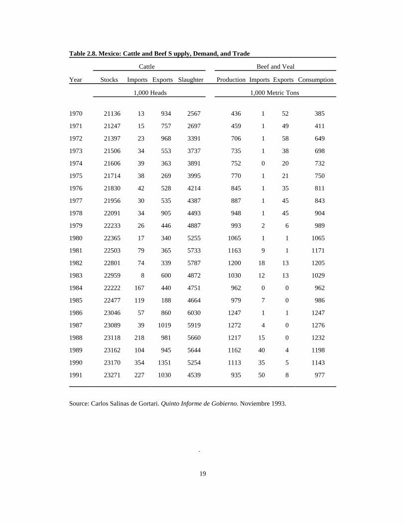
Mexican cattle trade has mainly consisted of feeder cattle exports and slaughter cattle imports. Mexican beef data reflectsthe good livestock production years of the 1970s and the bad years of the 1980s (Table 2.8). Production exceededconsumption until 1979 giving Mexico an opportunity to export beef. In the 1980s, however, Mexico became a netimporter of beef. Beef imports represented more than 3% of Mexican beef consumption between 1989 and 1991.Mexican beef production increased until 1982 only to fall during the following three years. In 1986, the Mexican beefindustry benefited from the decline of the domestic pork industry. Mexican beef production reached record levels in1986, 1987, and 1988 but has subsequently declined.
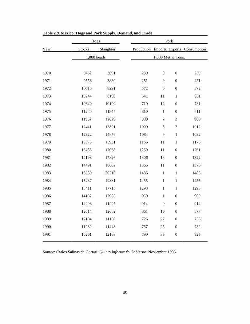
The Mexican Hog and Pork Industry
In contrast to the cattle industry where extensive production is most common, the Mexican hog and pork industry hasbecome more developed due to both national and foreign investment and the adoption of new technologies.Consequently, the hog industry has developed a solid structure independent of weather conditions. By late 1960s andearly 1970s, modern production techniques began to appear in the Mexican hog sector, mainly in the states of Sonoraand Sinaloa. Technological developments permitted the industry to reduce the amount of feed per kilogram (kg) ofweight gain from 5.5 kg in 1970 to 3.5 kg in 1980. Between 1960 and 1970, hog carcass weights increased from 62 kgto 70 kg per head (Gomez Cruz et al.)
The Mexican hog industry is composed of three types of production processes. The intensive or technified sectoraccounts for only 17% of the inventory but generates 35% of pork production in Mexico. The semi-technified sectoraccounts for 30% of the inventory and produces 35% of the meat. Finally, the rural or low technified sector accountsfor 53% of the inventory but contributes only 30% of the pork production (Gomez Cruz et al.)
From 1971 to 1983, hog slaughter grew more than 420% (Table 2.9). Pork production followed the same trend as wellas pork consumption. The following seven years, however, the industry experienced a decline due mainly to increasingcosts and a drop in prices. With the cancellation of the sorghum subsidy, by which livestock producers could obtain low-priced sorghum in Mexico, the cost of feeding hogs rose considerably driving a number of small and medium-sized hogfarms out of the industry. Hog inventories dropped more than 33% from 1983 to 1991, while pork production andconsumption fell 47% and 45%, respectively in over that period. Pork imports began to increase at the end of the 1980s.Imports accounted for 3% of pork consumption in 1989 and 1990 and about 4% in 1991.
The Mexican Chicken Industry
The poultry industry also experienced a rapid technological change that started in the 1950s. Feeding cycles werereduced and productivity increased as a result of imported management and breeding and feeding technologies. Also feedrequirements were reduced as in the case of hogs. In 1950, 4.5 kg of feed were required per kg of weight gain for poultryin Mexico. By 1988, only 2.1 kg were necessary per kg of weight gain, a drop of almost 55%. The feeding cycle of 91days in 1950 dropped to 56 days by 1985. The structure of the industry is defined by four kinds of producers: (1) smallindividual producers with 2,000 to 10,000 birds that do not produce their own feed and that have little or no access tothe main marketing channels; (2) associated producers, owners of 10,000 to 50,000 birds that mix their own feeds andthat have access to genetic material; (3) semi-integrated producers with 50,000 to 100,000 birds; and (4) large integratedenterprises with more than 100,000 birds (Gomez Cruz et al.)
Sorghum is one of the main components of the balanced feed used in the poultry and the hog industries in Mexico. Whenthe sorghum subsidy was eliminated in 1984, the poultry industry suffered a setback in the growth trend experiencedduring the 1970s and early 1980s. From 1970 to 1984, poultry meat production rose almost fourfold at an average annualrate of 11% (Table 2.10). The relative low cost of chicken helped to rise its consumption steadily over the last 30 years.Although chicken production did not drop as did pork production after 1984, consumption has outfaced production inMexico leading to an increase in imports. Imports represented more than 7% of total poultry consumption in 1988.
The Mexican Feed Industry
The dynamic development of the hog and poultry sectors made the development of the animal feed industry in Mexiconecessary. The Mexican animal feed industry first began to develop in about 1945. Over the period of 1960 to 1975, the
9
industry expanded at an annual rate of 14.1% while GDP grew at only 6.6% (Burst et al.). From 1970 to 1987, Mexicananimal feed production grew more than 57%. The main inputs of the Mexican feed industry are sorghum and soybeanmeal (soymeal). Sorghum represents 60% to 80% of mixed feeds while soymeal represents 15% to 20% (Gomez Cruzet al.). Although corn is considered a better input than sorghum from an animal nutrition standpoint, high governmentguaranteed corn prices and restrictions on the use of corn for feeding animals have limited its use as a feed ingredientin Mexico.
Mexican Sorghum Supply and Demand
Changes in the production of sorghum provide perhaps the best example of the Mexican orientation towards theproduction of livestock during the 1970s. Sorghum was produced on only 116,000 hectares (ha) in 1960 and accountedfor only 1.6% of the total harvested area in Mexico. However, by 1980 sorghum area reached 1.5 million ha and 10%of the total national area in 1979, second only to corn. The increase in production during that period, however, fell shortof consumption, leading to increases in imports of grain sorghum, especially in the late 1970s and early 1980s (Table2.11). In 1982, for example, imports accounted for almost 44% of total sorghum consumption in Mexico. With growingproduction and increasing imports, sorghum use almost tripled from 1970 to 1985. However, after the elimination of thesorghum subsidy in 1984, use fell almost 40% in 1986. By 1990, pressure from the growing livestock industry pushedsorghum consumption back to 1985 levels.
Mexican Soybeans and Soymeal Supply and Demand
Soybean meal is important to the Mexican mixed feed industry for use in balancing livestock rations. Sorghum andsoymeal rations provide a balanced ration of protein and energy for livestock. Harvested area of soybeans grew morethan 300% from 1970 to 1985 with a 285% increase in production during that period (Table 2.12). As in the case ofsorghum, the rate of growth of soybean consumption outfaced that of production, generating a need for imports. In thecase of soybeans, however, the gap between production and consumption was much larger. Imports represented almost60% of total soybean use during the 1980s. The use of soymeal has followed the same trend (Table 2.13). In 1984,soymeal consumption was more than six times that in 1970. Although increasing, imports have not been as importantfor soymeal as for sorghum or soybeans.
Mexican Corn Supply and Demand
Corn has been the main crop in Mexico for centuries. Most small farmers plant corn but much is consumed on-farm.Corn has been the most protected crop in Mexico. As a consequence, guaranteed prices have been normally higher forcorn than for any other crop, limiting its use as an animal feed. Imports have not accounted for a large proportion of totalcorn consumption. Corn prices averaged almost 60% more per MT than sorghum prices between 1970 and 1991 (Table2.14). NAFTA will likely boost Mexican corn imports which will increase corn supply and lower corn prices. This factwill make the use of corn as animal feed more attractive.
Mexican Agricultural Policy
Mexican agricultural policy has attempted to achieve two conflicting goals: (1) to increase agricultural output and theincomes of small farmers and (2) to provide low-priced food for poor, largely urban, consumers (Burst et al.). Mexicanland tenure laws have worked to prevent the attainment of those goals and have had a largely negative impact onagricultural production levels by limiting land per individual to only 500 ha (Bredahl et al.). Government interventionhas been manifest in several ways including public investment, price controls, subsidies, trade measures, etc. Engels andSegarra present a detailed description of the Mexican Government intervention in the livestock sector. Some of thefollowing discussion of Mexican agricultural policy implications for livestock and meat are based on their work. TheNorth American Free Trade Agreement (NAFTA) and the latest Mexican agricultural program (PROCAMPO) are alsodiscussed.
A much criticized regulation in the Mexican Constitution limited land holdings and improvements done on the landdevoted to livestock. This regulation impeded the vertical integration of livestock operations in Mexico in the past.

10
However, in November of 1991, a proposal was approved to reform several articles of the Constitution and modifies landtenure and improvement regulations as well as the structure and functioning of small land holdings (ejidos). This long-awaited measure had been delayed because of the potential political implications but was deemed to be an essential partof the Mexican government's economic reform program.
Public investment in the agricultural sector has been focused largely on irrigation development and technical assistance.Through the Comisión Nacional de Irrigación (National Irrigation Commission) and later the Secretaría de RecursosHidráulicos (Secretariat of Water Resources), the Mexican Government developed 827,000 ha of irrigated land duringthe period from 1926 to 1946. Irrigated area increased at an average annual rate of 7.2% during the 1940s and 1950s orslightly over 100,000 ha annually. This tendency slowed somewhat during the 1960s when the development of irrigatedland was about 65,000 ha per year. Irrigated area grew at an annual average of 80,000 ha in the 1970s. Technicalassistance has been provided free through extension services, although it is mainly available to small land holders(ejidatarios).
The policies that have most affected the livestock sector are price controls and supply management. Cattle and beefceiling prices have been set by the government at all levels in the market. Although pork and chicken meat prices arenot controlled, the substitutability between pork and chicken meat with beef has meant that price controls on beef haveaffected those prices as well (Engels and Segarra). Although beef is too expensive for low income groups despite pricecontrols, beef prices are the main indicator for pricing other meats and animal proteins. Because a maximum price forbeef is set to benefit consumers, the government has often had to allow imports to rise or restrict exports to relieveupward pressure on prices.
Mexican livestock trade policy has been neither very clear nor consistent over time. Allowing imports of cheap beef fromoverseas helps to keep prices low in Mexico. However, Mexican authorities often restrict beef imports to respond toproducer demands. At the same time, a quota on cattle exports (mainly feeder cattle) to the U.S. has existed but has oftenbeen modified according to domestic supplies. For example, in response to limited domestic supply and increased pricesin 1979, live cattle and beef exports to the U.S. were temporarily suspended (Bredahl et al.)
One of the most important agricultural policy instrument over the years has been the guaranteed price for the principalcrops produced in Mexico. This measure has allowed the government to increase or reduce the level of income ofagricultural producers and to change the product mix of agricultural output as needed. On several occasions, the state-runagricultural marketing board (CONASUPO) has subsidized feed and livestock producers selling crops at prices belowthe purchase price. Imports of feed inputs and of animal proteins have also been controlled by the government.Historically, government agencies like Conasupo have been responsible for grain imports and they could store or sellthe grain in order to enforce the guaranteed price policy (Burst et al.)
Credit has been subsidized through several official institutions especially to low and middle income producers. Officialbanks used to lend money sometimes below the average of costs paid by banks in Mexico. Undervaluation of the pesohas also been used as a trade policy to stimulate exports and reduce imports. Insurance, rail transportation, fuel (diesel),and genetic inputs like breeding stocks, are forms of subsidy given to Mexican producers, especially ejidatarios.
PROCAMPO is the latest of a series of measures intended to bring support to the Mexican agriculture. This innovativeprogram, however, includes direct support for farmers for the first time in Mexican agricultural policy. With this support,the Mexican Government intends to gradually eliminate the implicit subsidy that was in effect through guaranteed prices.This kind of support will be assigned on a hectare basis, thus reaching even those farmers that produce for self-consumption. Prices will likely decrease gradually until they reach the international level (Salinas, 1993). In this way,prices reflecting international levels will benefit consumers with low prices. Producers will receive a transfer from thegovernment regardless of prices or production levels.
Non-tariff border measures have played an important role in economic policy in Mexico. For example, 60% of the totalvalue of imports required import permits in 1980. However, although traditionally a protectionist country, Mexico starteda trade liberalization process in the mid-1980s. Mexico became the 92nd member of the General Agreement of Tariffsand Trade (GATT) in 1986. Searching for an economic realism that was absent in the 1970s and the early 1980s, Mexicoaccelerated its trade liberalization process in the late 1980s. By 1990, only a small number of products continued to have

an import permit requirement. Carlos Salinas de Gortari, who took office in December of 1988, continued the effortstoward freer trade. In April of 1990, a Mexican forum on the commercial relationships between Mexico and the worlddrew several important conclusions (Nacional Financiera). One of them was that commercial relationships with the U.S.and Canada should be strengthened, given the geographical proximity of those two countries. Given that a free tradeagreement (FTA) already existed between Canada and U.S., the possibility of signing an FTA between Mexico and U.S.seemed reasonable. Canada asked to be included in a three-way FTA. The North American Free Trade Agreement(NAFTA) was approved in 1993 by the three participant countries and entered in force on January 1, 1994.
NAFTA
The NAFTA intended to form a free trade zone of more than 360 million people with an estimated GNP of 6,000 billiondollars. This trade zone is now the largest free trade area in the world. NAFTA deals with a reduction of tariff and non-tariff barriers among these three countries without interfering in the commercial policies toward third countries. TheNAFTA is intended to gradually eliminate tariffs and non-tariff barriers and develop a just and rapid mechanism to solvecontroversies.
Several impacts are expected as a result of the NAFTA. Among the expected effects are an increase in the trade oflivestock and livestock products, with Mexican feeder cattle exports to the U.S. accounting for most of the expansion(Rosson et al.) Also, increased imports of processed meat by Mexico are expected, particularly if the expected increasein Mexican per capita incomes take place. If the U.S. has a comparative advantage in producing grains, as many say,Mexico could develop a grain-fed beef industry using cheaper grain from the U.S. and Mexican cheap labor. A phasedreduction of tariff barriers is expected. The section on simulation analysis provides an analysis of the likely implicationsof freer U.S.-Mexico trade for the Mexican livestock, meat, and feedgrain sectors.
Summary
This section has presented the characteristics of the Mexican livestock, meat and feedgrain sectors. Livestock and meatproduction flourished during the 1970s prompting the expansion of the feed sector. Beef has traditionally been the mainmeat consumed by Mexicans. However, during the mid-1970s to mid-1980s, pork had a bigger consumption share thanbeef. After the 1982 Mexican economic crisis, meat consumption decreased dramatically. Chicken emerged as a cheapalternative for beef and pork. Since the early 1980s, real meat and livestock prices have been declining consistently.Chicken prices, however, have dropping in real terms since the early 1970s. The Mexican government has influencedthe trade of livestock and meat as well as of the feedgrains. Sorghum and soymeal constitute the main components ofanimal feed in Mexico. Although corn is a close substitute for sorghum, price and Mexican regulations have limited itsuse as on animal feed. Cheap corn coming from the U.S. might mean more livestock consumption of corn.
PROCAMPO is the latest program of the Mexican government intervention in agriculture. This program, however,intends to gradually eliminate the guaranteed price scheme and to bring agricultural prices to a world level. Mexicangovernment has influenced the livestock and the feedgrain sectors mainly by imposing ceiling prices to beef and bycontrolling trade. However, Mexico started a trade liberalization in 1986 that resulted in the NAFTA.

12
Table 2.1. Mexico: Agriculture and Livestock Production as Percentage of Primary Sector andTotal GNP
Share of Primary GNP Share of Total GNP
Year Agriculture Livestock Agriculture Livestock Agr.+Liv.
% % % % %
1970 58.40 36.16 7.09 4.39 11.48
1971 59.42 35.43 7.17 4.28 11.45
1972 58.03 36.22 6.42 4.01 10.43
1973 57.89 36.49 6.71 4.23 10.94
1974 57.87 36.57 6.67 4.21 10.88
1975 57.21 37.35 6.37 4.16 10.53
1976 56.10 38.26 5.95 4.06 10.01
1977 57.30 36.61 6.02 3.85 9.87
1978 58.37 35.55 5.98 3.64 9.62
1979 56.12 37.06 5.14 3.40 8.54
1980 58.85 32.78 4.85 2.70 7.55
1981 59.77 31.90 4.80 2.56 7.36
1982 57.83 33.46 4.58 2.65 7.23
1983 58.45 33.34 4.73 2.70 7.43
1984 58.71 32.80 4.91 2.74 7.65
1985 59.73 31.92 5.05 2.70 7.75
1986 58.18 33.48 4.98 2.86 7.84
1987 58.97 32.09 5.04 2.74 7.78
1988 58.24 32.29 4.73 2.62 7.35
1989 58.52 31.89 4.48 2.44 6.92
1990 60.47 30.70 4.69 2.38 7.07
1991 60.00 31.25 4.53 2.36 6.89
Source: Carlos Salinas de Gortari. Quinto Informe de Gobierno. Noviembre 1993.

13
Table 2.2. Mexico: Meat Production. Mexican Data
Year Beef Pork Chicken Total
Thousands of Metric Tons
1970 436 239 74 749
1971 459 251 78 788
1972 706 572 215 1493
1973 735 641 229 1605
1974 752 719 248 1719
1975 770 810 269 1849
1976 845 909 288 2042
1977 887 1009 310 2206
1978 948 1084 335 2367
1979 993 1166 366 2525
1980 1065 1250 399 2714
1981 1163 1306 426 2895
1982 1200 1365 449 3014
1983 1030 1485 468 2983
1984 962 1455 489 2906
1985 979 1293 588 2860
1986 1247 959 672 2878
1987 1272 914 672 2858
1988 1217 861 627 2705
1989 1162 726 611 2499
1990 1113 757 750 2620
1991 1188 811 857 2856
Mean 960 935 428 2324
St. Dev. 241 347 213 688
Source: Carlos Salinas de Gortari. Quinto Informe de Gobierno. Noviembre 1993.

14
Table 2.3. Mexico: Meat Production. USDA Data
Year Beef Pork Chicken Total
Thousands of Metric Tons
1970 590 317 79 986
1971 581 351 84 1016
1972 625 573 241 1439
1973 664 651 245 1560
1974 700 731 285 1716
1975 1038 811 244 2093
1976 1079 735 271 2085
1977 990 653 280 1923
1978 1038 781 296 2115
1979 1116 838 328 2282
1980 1209 921 411 2541
1981 1271 852 446 2569
1982 1381 1009 467 2857
1983 1229 1136 435 2800
1984 1323 942 474 2739
1985 1339 865 502 2706
1986 1200 911 472 2583
1987 1205 950 409 2564
1988 1754 980 540 3274
1989 2140 937 633 3710
1990 1790 817 694 3301
1991 1670 855 781 3306
Mean 1179 801 392 2371
St Dev. 412 199 179 733
Source: Mexico: Livestock Data, PS&D View USDA/ERS 1992.

15
Table 2.4. Mexico: Per Capita Meat Consumption
Year Beef Pork Chicken Total
Thousands of Metric Tons
1970 7.60 4.71 1.46 13.77
1971 7.84 4.79 1.49 14.12
1972 11.96 10.54 3.96 26.46
1973 12.43 11.59 4.11 28.13
1974 12.59 12.58 4.30 29.47
1975 12.47 13.48 4.54 30.49
1976 13.08 14.67 4.73 32.48
1977 13.21 15.86 4.94 34.01
1978 13.77 16.63 5.19 35.59
1979 14.65 17.42 5.57 37.64
1980 15.29 18.10 5.90 39.29
1981 16.41 18.53 6.25 41.19
1982 16.50 18.84 6.31 41.65
1983 13.78 19.89 6.33 40.00
1984 12.61 19.07 6.53 38.21
1985 12.65 16.59 7.70 36.94
1986 15.67 12.06 8.62 36.35
1987 15.71 11.26 8.45 35.42
1988 14.87 10.59 8.17 33.63
1989 14.18 8.91 7.74 30.83
1990 13.27 9.08 9.10 31.45
1991 14.00 9.63 10.11 33.74
Source: Carlos Salinas de Gortari. Quinto Informe de Gobierno. Noviembre 1993.

16
Table 2.5. Mexico: Shares of Meat Consumption
Year Beef Pork Chicken
% % %
1970 55.19 34.20 10.61
1971 55.52 33.92 10.56
1972 45.20 39.83 14.97
1973 44.19 41.20 14.61
1974 42.72 42.69 14.59
1975 40.90 44.21 14.89
1976 40.27 45.16 14.57
1977 38.84 46.63 14.53
1978 38.69 46.73 14.58
1979 38.92 46.28 14.80
1980 38.92 46.07 15.01
1981 39.84 44.99 15.17
1982 39.62 45.23 15.15
1983 34.45 49.73 15.82
1984 33.00 49.91 17.09
1985 34.24 44.91 20.85
1986 43.11 33.18 23.71
1987 44.35 31.79 23.86
1988 44.22 31.49 24.29
1989 45.99 28.90 25.11
1990 42.19 28.87 28.94
1991 41.49 28.54 29.97
Source: Carlos Salinas de Gortari. Quinto Informe de Gobierno. Noviembre 1993.

17
Table 2.6. Mexico: Livestock and Meat Prices
Year FPC RPB FPH RPP RPCH
1978 Mexican Pesos
1970
16.04 56.10 28.40 54.10 36.04
1971 17.68 59.91 31.50 47.00 34.41
1972 17.29 61.04 31.90 52.10 36.26
1973 18.87 69.70 32.80 50.20 33.16
1974 21.70 63.66 33.20 46.70 33.12
1975 18.48 60.54 31.70 44.20 31.98
1976 19.64 52.38 29.50 40.50 31.77
1977 20.23 57.67 31.90 38.30 30.07
1978 19.74 62.95 35.50 39.20 30.14
1979 22.18 72.32 34.60 40.90 31.85
1980 22.13 65.83 37.00 46.30 32.38
1981 25.23 63.00 37.50 44.90 32.36
1982 24.78 70.17 40.00 48.60 24.79
1983 26.38 61.86 36.10 43.40 23.83
1984 20.21 73.90 38.60 45.20 21.60
1985 21.14 71.34 37.00 42.80 22.77
1986 24.87 91.31 36.92 37.63 22.57
1987 24.46 54.39 30.50 33.61 20.83
1988 22.47 57.18 25.53 34.28 22.02
1989 23.69 65.94 22.68 42.00 22.24
1990 17.59 57.39 21.75 36.62 23.56
1991 19.32 53.99 21.77 38.57 21.12
Note: FPC = Farm Price of Cattle.
RPB = Retail Price of Beef.
FPH = Farm Price of Hogs.
RPP = Retail Price of Pork.
RPCH = Retail Price of Chicken.
Source: Roberto Garcia Mata.

18
Table 2.7. Mexico: Livestock Inventories
Cattle Inventories Hog Inventories
Year (1) (2) (3) (1) (2) (3)
1,000 Heads
1970 25499 21136 24876 10541 9462 10297
1971 26265 21247 26053 10747 9555 9970
1972 27335 21397 27335 11372 10015 11372
1973 28103 21506 28105 11743 10244 11743
1974 28816 21606 28816 12313 10639 12313
1975 29602 21714 29200 13179 11280 13179
1976 30461 21830 29900 14097 11951 14100
1977 31410 21956 30410 14814 12440 14200
1978 32439 22091 31300 15534 12921 15534
1979 33545 22233 32150 16233 13375 16200
1980 34590 22365 33000 16890 13784 16680
1981 35689 22503 34000 17562 14197 16480
1982 37191 22801 34700 18096 14490 17150
1983 37522 22959 33873 19364 15359 16460
1984 30374 22222 33917 19393 15236 13137
1985 31489 22477 33853 17233 13411 12320
1986 35237 23046 32167 18397 14181 13115
1987 34565 23089 33603 18722 14295 12357
1988 33756 23118 35378 15884 12013 10879
1989 33068 23162 34999 16157 12104 9003
1990 32054 23170 31747 15203 11281 8563
1991 31822 23271 30005 15902 10260 8593
Mean 1856 22314 31336 15426 12386 31336
St. Dev. 3344 696 2998 2781 1865 2722
Sources: (1) Carlos Salinas. Cuarto Informe de Gobierno. Noviembre 1992.
(2) Carlos Salinas. Quinto Informe de Gobierno. Noviembre 1993.
(3) USDA. PS&D View.
19
Table 2.8. Mexico: Cattle and Beef S upply, Demand, and Trade
Cattle Beef and Veal
Year Stocks Imports Exports Slaughter Production Imports Exports Consumption
1,000 Heads 1,000 Metric Tons
1970 21136
13 934
2567 436
1 52
385
1971 21247 15 757 2697 459 1 49 411
1972 21397 23 968 3391 706 1 58 649
1973 21506 34 553 3737 735 1 38 698
1974 21606 39 363 3891 752 0 20 732
1975 21714 38 269 3995 770 1 21 750
1976 21830 42 528 4214 845 1 35 811
1977 21956 30 535 4387 887 1 45 843
1978 22091 34 905 4493 948 1 45 904
1979 22233 26 446 4887 993 2 6 989
1980 22365 17 340 5255 1065 1 1 1065
1981 22503 79 365 5733 1163 9 1 1171
1982 22801 74 339 5787 1200 18 13 1205
1983 22959 8 600 4872 1030 12 13 1029
1984 22222 167 440 4751 962 0 0 962
1985 22477 119 188 4664 979 7 0 986
1986 23046 57 860 6030 1247 1 1 1247
1987 23089 39 1019 5919 1272 4 0 1276
1988 23118 218 981 5660 1217 15 0 1232
1989 23162 104 945 5644 1162 40 4 1198
1990 23170 354 1351 5254 1113 35 5 1143
1991 23271 227 1030 4539 935 50 8 977
Source: Carlos Salinas de Gortari. Quinto Informe de Gobierno. Noviembre 1993.
.
20
Table 2.9. Mexico: Hogs and Pork Supply, Demand, and Trade
Hogs Pork
Year Stocks Slaughter Production Imports Exports Consumption
1,000 heads 1,000 Metric Tons.
1970 9462 3691 239 0 0 239
1971 9556 3880 251 0 0 251
1972 10015 8291 572 0 0 572
1973 10244 8190 641 11 1 651
1974 10640 10199 719 12 0 731
1975 11280 11345 810 1 0 811
1976 11952 12629 909 2 2 909
1977 12441 13891 1009 5 2 1012
1978 12922 14876 1084 9 1 1092
1979 13375 15931 1166 11 1 1176
1980 13785 17058 1250 11 0 1261
1981 14198 17826 1306 16 0 1322
1982 14491 18602 1365 11 0 1376
1983 15359 20216 1485 1 1 1485
1984 15237 19881 1455 1 1 1455
1985 13411 17715 1293 1 1 1293
1986 14182 12963 959 1 0 960
1987 14296 11997 914 0 0 914
1988 12014 12662 861 16 0 877
1989 12104 11180 726 27 0 753
1990 11282 11443 757 25 0 782
1991 10261 12163 790 35 0 825
Source: Carlos Salinas de Gortari. Quinto Informe de Gobierno. Noviembre 1993.

21
Table 2.10. Mexico: Chicken Supply, Demand, and Trade
Year Production Imports Consumption
1,000 Metric Tons
1970 74 0 74
1971 78 0 78
1972 215 0 215
1973 229 2 231
1974 248 2 250
1975 269 4 273
1976 288 5 293
1977 310 5 315
1978 335 6 341
1979 366 10 376
1980 399 12 411
1981 426 20 446
1982 449 12 461
1983 468 5 473
1984 489 9 498
1985 588 12 600
1986 672 14 686
1987 672 14 686
1988 627 50 677
1989 611 45 656
1990 750 39 789
1991 857 37 894
Source: Carlos Salinas de Gortari. Quinto Informe de Gobierno. Noviembre 1993.

22
Table 2.11. Mexico: Sorghum Production, Consumption, Trade, and Prices
Year Harv. Area Production Imp. (Exp.) Consumption Price
1,000 Has. 1,000 Metric Tons 1978 Pesos
1970 971 2747 (18) 2729 34000
1971 937 2565 (21) 2544 34050
1972 1109 2612 246 2858 35048
1973 1185 3270 13 3283 35333
1974 1156 3459 466 3925 43724
1975 1445 4126 835 4961 49188
1976 1251 4027 44 4071 42564
1977 1413 4325 715 5040 35679
1978 1399 4193 752 4945 35094
1979 1164 3958 1293 5251 32908
1980 1543 4689 2252 6941 36684
1981 1684 5086 3631 8717 33551
1982 1434 4712 3646 8358 33962
1983 1528 4867 3330 8197 32097
1984 1636 5038 2311 7349 37255
1985 1862 6597 2222 8819 34160
1986 1533 4833 782 5615 43413
1987 1853 6298 766 7064 34522
1988 1800 5835 1207 7042 35839
1989 1620 5002 2665 7667 33236
1990 1820 5978 2856 8834 29760
1991 1340 4308 3200 7508 32312
Source: Carlos Salinas de Gortari. Quinto Informe de Gobierno. Noviembre 1993. Canacintra.

23
Table 2.12. Mexico: Soybeans Production, Consumption, Trade, and Prices
Year Harv. Area Production Imp. (Exp.) Consumption Price
1,000 Has. 1,000 Metric Tons 1978 Pesos
1970 112 215 102 317 86053
1971 128 255 68 323 82900
1972 222 377 11 388 85381
1973 312 565 62 627 126250
1974 300 491 435 926 113690
1975 344 599 22 621 104688
1976 172 302 348 650 106436
1977 314 515 526 1041 93071
1978 217 334 681 1015 89484
1979 379 707 589 1296 85434
1980 154 322 522 844 80958
1981 362 707 1110 1817 91415
1982 383 645 485 1130 83076
1983 391 688 883 1571 85793
1984 389 685 1308 1993 89754
1985 476 829 1319 2148 86064
1986 381 709 827 1536 86825
1987 470 828 1062 1890 104528
1988 139 225 1099 1324 84123
1989 490 932 1170 2102 91751
1990 286 575 897 1472 64443
1991 326 725 1489 2214 63076
Source: Carlos Salinas de Gortari. Quinto Informe de Gobierno. Noviembre 1993. Canacintra.
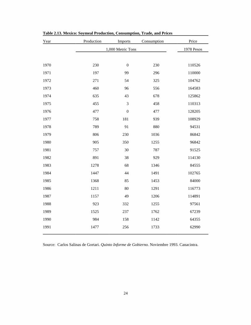
24
Table 2.13. Mexico: Soymeal Production, Consumption, Trade, and Prices
Year Production Imports Consumption Price
1,000 Metric Tons 1978 Pesos
1970 230 0 230 110526
1971 197 99 296 110000
1972 271 54 325 104762
1973 460 96 556 164583
1974 635 43 678 125862
1975 455 3 458 110313
1976 477 0 477 128205
1977 758 181 939 108929
1978 789 91 880 94531
1979 806 230 1036 86842
1980 905 350 1255 96842
1981 757 30 787 91525
1982 891 38 929 114130
1983 1278 68 1346 84555
1984 1447 44 1491 102765
1985 1368 85 1453 84000
1986 1211 80 1291 116773
1987 1157 49 1206 114891
1988 923 332 1255 97561
1989 1525 237 1762 67239
1990 984 158 1142 64355
1991 1477 256 1733 62990
Source: Carlos Salinas de Gortari. Quinto Informe de Gobierno. Noviembre 1993. Canacintra.
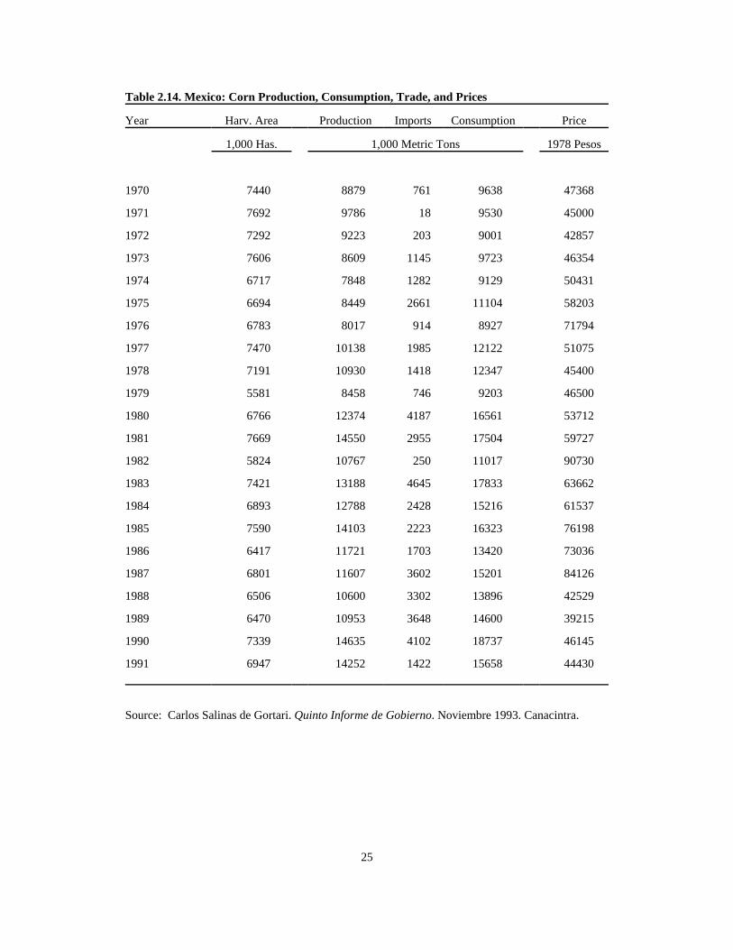
25
Table 2.14. Mexico: Corn Production, Consumption, Trade, and Prices
Year Harv. Area Production Imports Consumption Price
1,000 Has. 1,000 Metric Tons 1978 Pesos
1970 7440 8879 761 9638 47368
1971 7692 9786 18 9530 45000
1972 7292 9223 203 9001 42857
1973 7606 8609 1145 9723 46354
1974 6717 7848 1282 9129 50431
1975 6694 8449 2661 11104 58203
1976 6783 8017 914 8927 71794
1977 7470 10138 1985 12122 51075
1978 7191 10930 1418 12347 45400
1979 5581 8458 746 9203 46500
1980 6766 12374 4187 16561 53712
1981 7669 14550 2955 17504 59727
1982 5824 10767 250 11017 90730
1983 7421 13188 4645 17833 63662
1984 6893 12788 2428 15216 61537
1985 7590 14103 2223 16323 76198
1986 6417 11721 1703 13420 73036
1987 6801 11607 3602 15201 84126
1988 6506 10600 3302 13896 42529
1989 6470 10953 3648 14600 39215
1990 7339 14635 4102 18737 46145
1991 6947 14252 1422 15658 44430
Source: Carlos Salinas de Gortari. Quinto Informe de Gobierno. Noviembre 1993. Canacintra.

26
CONCEPTUAL MODEL OF THE MEXICAN LIVESTOCK, MEAT, AND FEEDGRAIN SECTORS
This section lays out the conceptual model of the Mexican livestock, meat, and feed sectors. First, the underlyingassumptions and the conceptual framework used to construct the model are discussed. Then, the livestock and meatsupply model component is presented followed by the feed supply and demand component of the model. Threealternative specifications for the meat demand model component and their characteristics are discussed later. Finally,the full conceptual model which integrates the livestock and meat supply component with each of the alternative meatdemand model components is laid out and discussed in detail. The full conceptual model is the basis for the statisticalmodel estimated in the empirical analysis section and used in the simulation analysis section to analyze the likely effectsof the freer U.S.-Mexico trade on the Mexican livestock, meat, and feedgrain markets.
The complete Mexican livestock, meat, and feedgrain model includes ten commodities: three types of livestock (cattle,hogs, and chicken), three types of meat (beef, pork, and chicken meat), and four feeds (sorghum, soybean, soymeal, andcorn). For every commodity there is a set of equations depicting behavioral relationships of supply and demand and amarket clearing condition. The conceptual framework for each group of commodities (livestock, meat, and feeds) willfirst be discussed in general terms.
Underlying Assumptions of the Mexican Livestock, Meat, and Feedgrain Model
As discussed in the background section, the Mexican government has set quotas on imports and exports of beef and cattlein the past as a means of controlling beef prices. Whenever there was a threat of raising beef prices because of a decreasein the domestic beef supply, the Mexican government tended to restrict cattle exports and to open the border to beefimports. A similar situation occurs with feedgrains. Controls on imports of feed inputs and of animal proteins have beenused by the Mexican government to enforce the "guaranteed price" policy. Although the situation is changing underNAFTA, the import and export of most agricultural products have been controlled by the government via permits and/ortariffs. The practical implications of these policies for modeling purposes is that imports and exports can be assumedto have been exogenously determined over much of the historical period. Animal bearing rates and production yieldsdepend on technology developments which are also exogenous to this model. Input costs and credit availability, as wellas non-feed use of feeds are also assumed to be exogenous. Weights used in the calculation of grain consuming animalunits are also assumed to be determined by technology and, therefore, exogenous. Finally, economic and demographicvariables such as consumer price index, wholesale price index, total population, and real per capita income areconsidered to be exogenous to the Mexican livestock and feed sectors.
Conceptual Framework for Livestock
The livestock supply system includes cattle, hogs, and chicken. The well-known work of Jarvis provides a frameworkfor treating livestock inventories as capital goods and farmers as portfolio managers. Farmers are assumed to base theirdecisions about livestock breeding herd size on the expected profitability of raising animals. The breeding herd size isassumed to adjust slowly to the desired optimum long-run level. At the same time, profit expectations are assumed tobe updated each time period based on the current forecasting error. Under this set of assumptions and following someother studies (Wahl, Gong, Tsai), producer decisions may be represented by the following theoretical breeding herdinventory model:
(3.1) H*t = ƒ(Ae
t-1,Zt),
where H*t is the desired breeding herd size at the end of period t, Ae
t-1 represents the expected profitability of raisinglivestock in the following period, and Z represents other exogenous variables that occur at time period t that mayinfluence the level of desired inventory.
Assuming a partial adjustment framework and adaptive price expectations, equation (3.1) may be derive to:

27
(3.2a) Ht - Ht-1 = J(H*t - Ht-1) (0 # J #1) and
(3.2b) Aet-1 - Ae
t = L(At - Aet) (0 # L #1),
where J is the coefficient of adjustment and L is the coefficient of expectation. Equation (3.2a) suggests that the breedinginventory herd adjusts only partially each period due to biological restrictions and adjustment costs. Equation (3.2b)assumes that the change in expected profit in period t+1 is proportional to the current error in forecasting.
Assuming a linear form and combining (3.1), (3.2a), and (3.2b) the breeding herd equation is estimated as follows:(3.3) H = a0 + a1A + a2Ht-1 + a3Ht-2 + a4Z + a5Zt-1,where a0 = JL",
a1 = JL$,a2 = [(1-J) + (1-L)],a3 = (1-J)(1-L),a4 = J,,a5 = J(1-L),.
Also, " is the intercept and $ and , are the coefficients of the variables in the linear form of (3.1).
Feeder livestock inventories each year depend upon the offspring born in current and past periods. As a biological limit,cows generally have only one offspring per year while swine may bear more than one in the same period. Offspring,which are the supply of "new animals", are determined by the beginning breeding herd inventory and the bearing rate.Hence, the offspring born and the feeder inventory are modeled as:
(3.4) Off = H * BR(3.5) F = F(Off, Offt-1),
where Off represents the livestock offspring born, BR is the bearing rate, F is the ending feeder inventory, and H is stillbreeding inventory.
Farmers decide upon the usage of the available supply of livestock based on their profit expectations. Following Jarvis,livestock may be used for slaughter or can be held in inventory depending upon price behavior. If the farm price oflivestock is high, then farmers might follow an investment behavior, that is, farmers may hold animals in inventory inorder to profit from future greater inventories. On the other hand, if the retail price of meat is high, farmers will sendmore livestock to slaughter to take advantage of higher current output prices. In addition, the greater the supply ofanimals available (beginning feeder inventories), the more animals that can be slaughtered. Hence, slaughter livestockbehavior is specified as follows:
(3.6) Sl = Sl(RPM, FPL, Ft-1),
where Sl is the total number of animals slaughtered, RPM represents the retail price of the meat, FPL is the farm priceof the livestock, and all other variables are as defined before.
Market clearing conditions require total supply to be equal to total demand. Total supply of livestock in a given periodis composed of beginning inventories of both breeding and feeder livestock, the offspring born during the period, andlivestock imports. Total demand for livestock is the summation of livestock slaughter, total ending inventories, andlivestock exports. The residual of this identity is accounted for by livestock loss and statistical discrepancy. The marketclearing condition for livestock can be specified as:
(3.7) Ht-1 + Ft-1 + Off + Ml = Sl + H + F + Xl + LD,
where Ml and Xl are livestock imports and exports, respectively, LD is the loss and statistical discrepancy, and all othervariables as defined earlier.

28
Because the reproductive cycle for chicken is only five to six weeks, chicken inventory behavior cannot be consideredwithin an annual model. Slaughter of chicken, however, can be modeled to capture profit expectations of farmers. If chicken prices raise, farmers are encouraged send more chicken to slaughter. The opposite is true if the price of feed goesup. Hence, chicken slaughter behavior may be modeled as:
(3.8) Slch = Slch(RPch, PF, Z),
where Slch represents slaughter of chicken, RPch is the retail price of chicken, PF is the price of feed, and Z representother factors such as technological change.
Conceptual Framework for Meat
Meat production depends upon slaughter. The higher the slaughter of animals the greater the production of meat. Thetotal supply of meat includes both meat production and imports of meat. Per capita demand for meat is expected to beinfluenced by the own price of the respective meat, the prices of substitute meats, and the level of per capita income.Specification for meat demand is widely discussed later in this section. The supply, demand, and the market clearingcondition for each meat type is defined as follows:
(3.9) TPM = Sl * CW(3.10) PDM = TDM / Pop(3.11) PDM = PDM(RPM, RPS1, RPS2, PI)(3.12) TPM + MM = TDM + XM,
where TPM is total production of meat. CW represents the livestock average carcass weight. PDM denotes per capitademand of meat. TDM means total demand for meat. Pop indicates total population. RPS1 and RPS2 are the price ofsubstitutes one and two, respectively. PI represents per capita income. MM and XM are imports and exports of meat,respectively. All other variables as defined earlier.
Conceptual Framework for Feedgrains
As Gomez Cruz et al. state, sorghum and soymeal represent roughly 90% of livestock mixes in Mexico. Although officialregulations limit its use as animal feed input, corn is considered (and frequently used) as a substitute for sorghum. Thebehavior of the feed industry has been highly influenced by the livestock industry (see background section). For instance,feed demand behavior has been mainly determined by the behavior of livestock inventories. The price of the respectivefeed and the price of substitute feeds also affect quantities demanded. Feed supply is determined by area planted andyield of the respective crops. The area planted of each crop is determined mainly by farmer's profit expectations. Farmersare normally assumed to follow naive expectation pattern, i.e. the desired current planted area of a given feedgrain isa function of lagged profit from producing the feedgrain and other exogenous variables like expected weather and creditavailability. The area harvested is a function of the planted area. Crop production is determined by the area harvestedtimes a technologically determined crop yield. As mentioned before, this factor is considered to be exogenouslydetermined.
The supply model for sorghum, soybean, and corn can be, thus, specified as:
(3.13) AP = AP(APt-1, PFt-1, Z)(3.14) AH = AH(AP)(3.15) TPF = AH * CY,
where AP symbolizes area planted; PF means price of feed; Z represents some exogenous variables such as rain, inputcosts, or available credit; AH is area harvested; TPF is total production of feed; and CY is the crop yield per unit of area.
Production of soymeal follows a different behavior since it depends on the amount of soybean crushed. Hence, thespecification for soymeal production is:

29
(3.16) PSM = CDSB * SMY,
where PSM symbolizes production of soymeal, CDSB is the crush demand for soybeans explained later, and SMY isthe meal yield factor obtained from soybeans.
Feed demand for sorghum, soymeal, and corn is presented next. As discussed earlier, feed demand is affected by thenumber of grain consuming animal units, the price of the specific feed, and the prices of substitute feeds. Grainconsuming animal units is the number of livestock and poultry animals weighted by the roughage consumption factorsdeveloped for high-energy, low-fiber feeds (ERS-USDA S.B.#530). Feed demand is specified as:
(3.17) FD = FD(GCA, PF, Pfs),
where FD is feed demand; GCA represents grain consuming animal units; PF is feed price; and PFs is the price of asubstitute feed.
Soybean demand is structured differently due to its characteristic as an intermediate good. Crush demand for soybeansis affected by input and output prices. Also, availability of soybeans and installed capacity for crushing should have astrong influence on the volume of soybeans crushed. The crush demand for soybeans is specified as follows:
(3.18) CDSB = CDSB(PSB, PSM, SSB, CC),
where CDSB is as defined earlier; PSB is the input price (soybean price); PSM is the output price (soymeal price); SSBmeans supply of soybeans; and CC indicates crush capacity.
The market clearing conditions for each feed would be specified as:
(3.19) MF + TPF = FD + NFD + XF,
where MF and XF represent imports and exports of feed, respectively; NFD indicates non-feed demand; and the rest ofthe variables as defined earlier.
The Mexican Livestock and Meat Supply Model
Figure 3.1, 3.2, and 3.3 depict the flow of relationships for the cattle and beef, hog and pork, and chicken and chickenmeat industries, respectively. Circles are used to indicate the variables that are estimated within the model (endogenousvariables) while squares indicate those variables that are determined independently of the model estimation (exogenousvariables). Dashed lines indicate a lagged relationship among variables.
Total cattle supply is composed by lagged feeder and breeding inventories, the calves born, and the imports of cattle(Figure 3.1). The supply of cattle either remains on inventory or is slaughtered or exported. Cattle loss and statisticaldiscrepancy is shown as a residual. The number of calves born are determined by the inventory of breeding cattle andthe bearing rate. Cattle breeding inventories are affected by the farm price of cattle, the producer price of feed whichcomes from the feed model, and by other exogenous variables. Farm price of cattle and retail price of beef as well aslagged supply of total cattle determine the number of slaughtered cattle. The cattle slaughtered and the average carcassweight determine the total production of beef. Total supply of beef is composed by total production and imports of beef.Consumption of beef is affected by retail prices of beef, pork, and chicken and by per capita income as shown in Figure3.1.
Figure 3.2 depicts the behavioral relationships for the hog and pork sectors in a similar way to cattle and beef. Chickenand chicken meat sector behavior is described in Figure 3.3. Slaughter of chicken is influenced by the farm price of feed(determined in the feed model), the retail price of chicken and other exogenous factors. Chicken meat production dependsdirectly upon the number of slaughtered chickens and the technologically determined chicken average carcass weight.Chicken consumption, as in the case of beef and pork, is affected by the prices of chicken, beef, and pork and per capitaincome.

30
Table 3.1 contains the set of equations that illustrate the supply behavior of the Mexican livestock and meat sectors.Equation [3.1] follows the behavior of the general livestock equation (3.3). Ending inventory of breeding cattle is afunction of the expected profit of raising cattle as represented by the ratio of farm price of cattle (FPC) and the producerprice of feed (PPF). Lagged breeding inventories and some exogenous variables (Z) also affect the breeding herd sizedecision of farmers. Ending inventories of feeder cattle in a given year (EIFC) are modeled, following eq. (3.4), as afunction of the number of calves born during the present and past periods (equation [3.3]). Calves born are determinedby multiplying the beginning inventory of breeding cattle and the corresponding calving rate factor (CR), as shown ineq. [3.2] in Table 3.1.
Equation [3.4] in Table 3.1 specifies the slaughter behavior for cattle (SLTC). The retail price of beef (RPB), the farmprice of cattle (FPC), and the available supply of slaughter animals (EIFC) determine the level of cattle slaughter eachyear. This behavior was described in equation (3.6) in the previous section. The market clearing condition for cattle isgiven in equation [3.5] in Table 3.1.
Beef production is presented in equation [3.6] in Table 3.1 following the specification of text equation (3.9) in theprevious section. Total production of beef (TPB) is obtained by multiplying the amount of cattle slaughtered and theaverage carcass weight (CACW).
The demand for beef as shown on figure 3.1 is affected by beef, pork, and chicken prices and by per capita income. Asexplained earlier, demand specifications will be discussed in more detail later. The market clearing condition for beefis shown in equation [3.7].
The hog and pork sector behaves in a similar fashion to that of cattle and beef. Ending breeding inventories of sows(EIBS) (equation [3.8] in Table 3.1) and ending feeder pig inventories (EIFP) (equation[3.9] in Table 3.1) follow thesame specification as equations [3.1] and [3.2] for the cattle sector. The expected profit for raising hogs (FPH/PPF),lagged inventories, and exogenous variables (Z) influence farmers' decisions about hog breeding herd size (equation[3.8]in Table 3.1).
The number of piglets born (PB) is determined by the product of breeding inventories (EIBS) and the birth rate of pigs(PR) (equation [3.9] in Table 3.1). The slaughter of all hogs (SLHG) is a function of the farm price of hogs (FPH), theretail price of pork (RPP), and feeder pig inventories (EIFP) (equation [3.10] in Table 3.1).
Equation [3.12] is the hogs market clearing identity. Beginning inventories of feeder and breeding hogs plus piglets bornand the imports of hogs constitute the supply of animals in the hog industry. The demand for hogs includes hog slaughter,exports of hogs, and ending inventories of feeder and breeding inventories. Again, loss and statistical discrepancy (LD)constitute the residual in the market clearing condition.
Total production of pork (TPP) is the product of the number of hogs slaughtered and the average carcass weight of hogs(HACW)(equation [3.13] in Table 3.1). Equation [3.14] is the market clearing condition for pork.
The slaughter of chickens is specified to be a function of the retail price of chicken (RPCH), the producer price of feed(PPF), and some exogenous factor (Z) (equation [3.15] in Table 3.1). Total production of chicken meat (TPCH) is theproduct of the number of chickens slaughtered (SLCH) and their average carcass weight (CHCW) (equation [3.16] inTable 3.1). Finally, equation [3.19] is the market clearing condition for chicken meat.
The Mexican Feed Supply and Demand Model
Figure 3.4 presents a flow chart indicating the relationships within the feed sector and between the feed and the livestockmodel. Area planted of sorghum, soybean, and corn are affected by lagged farm prices and input costs. The area plantedof a crop determines the corresponding area harvested. Production of a particular feed is determined by the area harvestedand the production yield per hectare (Figure 3.4). Feed demand is affected by prices and by the number of grainconsuming animal units which is determined within the livestock sector. A weighted average of prices determine theproducer price of feed which feeds into the livestock sector as discussed before.
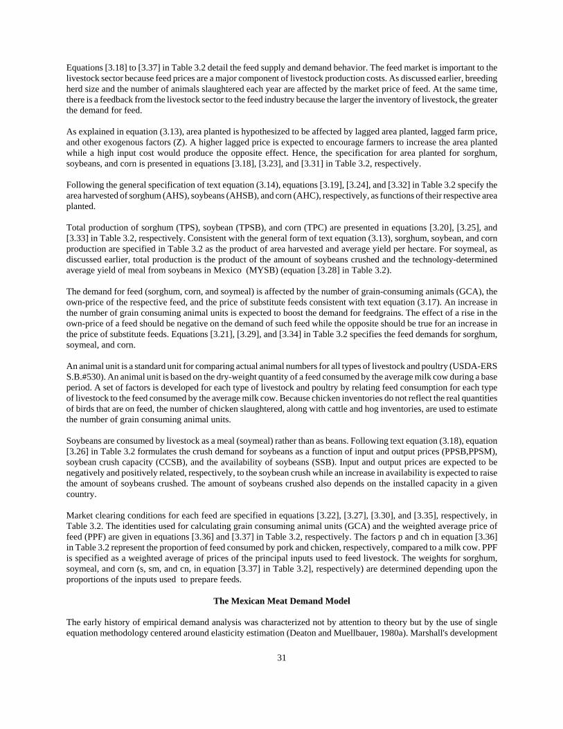
31
Equations [3.18] to [3.37] in Table 3.2 detail the feed supply and demand behavior. The feed market is important to thelivestock sector because feed prices are a major component of livestock production costs. As discussed earlier, breedingherd size and the number of animals slaughtered each year are affected by the market price of feed. At the same time,there is a feedback from the livestock sector to the feed industry because the larger the inventory of livestock, the greaterthe demand for feed.
As explained in equation (3.13), area planted is hypothesized to be affected by lagged area planted, lagged farm price,and other exogenous factors (Z). A higher lagged price is expected to encourage farmers to increase the area plantedwhile a high input cost would produce the opposite effect. Hence, the specification for area planted for sorghum,soybeans, and corn is presented in equations [3.18], [3.23], and [3.31] in Table 3.2, respectively.
Following the general specification of text equation (3.14), equations [3.19], [3.24], and [3.32] in Table 3.2 specify thearea harvested of sorghum (AHS), soybeans (AHSB), and corn (AHC), respectively, as functions of their respective areaplanted.
Total production of sorghum (TPS), soybean (TPSB), and corn (TPC) are presented in equations [3.20], [3.25], and[3.33] in Table 3.2, respectively. Consistent with the general form of text equation (3.13), sorghum, soybean, and cornproduction are specified in Table 3.2 as the product of area harvested and average yield per hectare. For soymeal, asdiscussed earlier, total production is the product of the amount of soybeans crushed and the technology-determinedaverage yield of meal from soybeans in Mexico (MYSB) (equation [3.28] in Table 3.2).
The demand for feed (sorghum, corn, and soymeal) is affected by the number of grain-consuming animals (GCA), theown-price of the respective feed, and the price of substitute feeds consistent with text equation (3.17). An increase inthe number of grain consuming animal units is expected to boost the demand for feedgrains. The effect of a rise in theown-price of a feed should be negative on the demand of such feed while the opposite should be true for an increase inthe price of substitute feeds. Equations [3.21], [3.29], and [3.34] in Table 3.2 specifies the feed demands for sorghum,soymeal, and corn.
An animal unit is a standard unit for comparing actual animal numbers for all types of livestock and poultry (USDA-ERSS.B.#530). An animal unit is based on the dry-weight quantity of a feed consumed by the average milk cow during a baseperiod. A set of factors is developed for each type of livestock and poultry by relating feed consumption for each typeof livestock to the feed consumed by the average milk cow. Because chicken inventories do not reflect the real quantitiesof birds that are on feed, the number of chicken slaughtered, along with cattle and hog inventories, are used to estimatethe number of grain consuming animal units.
Soybeans are consumed by livestock as a meal (soymeal) rather than as beans. Following text equation (3.18), equation[3.26] in Table 3.2 formulates the crush demand for soybeans as a function of input and output prices (PPSB,PPSM),soybean crush capacity (CCSB), and the availability of soybeans (SSB). Input and output prices are expected to benegatively and positively related, respectively, to the soybean crush while an increase in availability is expected to raisethe amount of soybeans crushed. The amount of soybeans crushed also depends on the installed capacity in a givencountry.
Market clearing conditions for each feed are specified in equations [3.22], [3.27], [3.30], and [3.35], respectively, inTable 3.2. The identities used for calculating grain consuming animal units (GCA) and the weighted average price offeed (PPF) are given in equations [3.36] and [3.37] in Table 3.2, respectively. The factors p and ch in equation [3.36]in Table 3.2 represent the proportion of feed consumed by pork and chicken, respectively, compared to a milk cow. PPFis specified as a weighted average of prices of the principal inputs used to feed livestock. The weights for sorghum,soymeal, and corn (s, sm, and cn, in equation [3.37] in Table 3.2], respectively) are determined depending upon theproportions of the inputs used to prepare feeds.
The Mexican Meat Demand Model
The early history of empirical demand analysis was characterized not by attention to theory but by the use of singleequation methodology centered around elasticity estimation (Deaton and Muellbauer, 1980a). Marshall's development
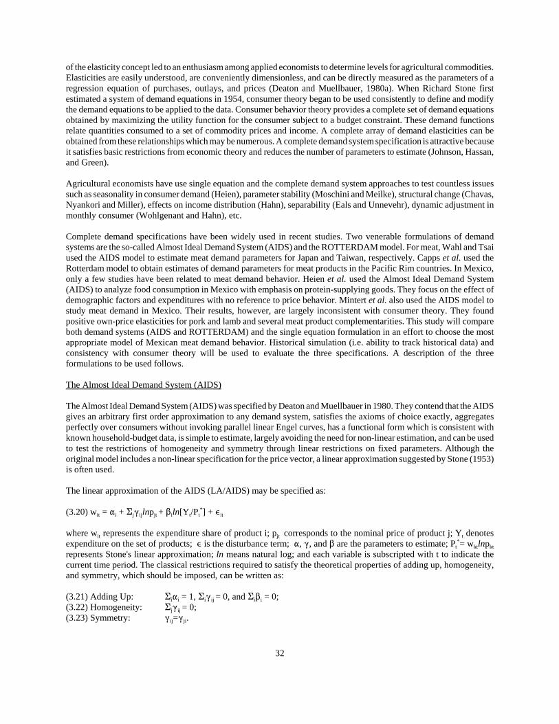
32
of the elasticity concept led to an enthusiasm among applied economists to determine levels for agricultural commodities.Elasticities are easily understood, are conveniently dimensionless, and can be directly measured as the parameters of aregression equation of purchases, outlays, and prices (Deaton and Muellbauer, 1980a). When Richard Stone firstestimated a system of demand equations in 1954, consumer theory began to be used consistently to define and modifythe demand equations to be applied to the data. Consumer behavior theory provides a complete set of demand equationsobtained by maximizing the utility function for the consumer subject to a budget constraint. These demand functionsrelate quantities consumed to a set of commodity prices and income. A complete array of demand elasticities can beobtained from these relationships which may be numerous. A complete demand system specification is attractive becauseit satisfies basic restrictions from economic theory and reduces the number of parameters to estimate (Johnson, Hassan,and Green).
Agricultural economists have use single equation and the complete demand system approaches to test countless issuessuch as seasonality in consumer demand (Heien), parameter stability (Moschini and Meilke), structural change (Chavas,Nyankori and Miller), effects on income distribution (Hahn), separability (Eals and Unnevehr), dynamic adjustment inmonthly consumer (Wohlgenant and Hahn), etc.
Complete demand specifications have been widely used in recent studies. Two venerable formulations of demandsystems are the so-called Almost Ideal Demand System (AIDS) and the ROTTERDAM model. For meat, Wahl and Tsaiused the AIDS model to estimate meat demand parameters for Japan and Taiwan, respectively. Capps et al. used theRotterdam model to obtain estimates of demand parameters for meat products in the Pacific Rim countries. In Mexico,only a few studies have been related to meat demand behavior. Heien et al. used the Almost Ideal Demand System(AIDS) to analyze food consumption in Mexico with emphasis on protein-supplying goods. They focus on the effect ofdemographic factors and expenditures with no reference to price behavior. Mintert et al. also used the AIDS model tostudy meat demand in Mexico. Their results, however, are largely inconsistent with consumer theory. They foundpositive own-price elasticities for pork and lamb and several meat product complementarities. This study will compareboth demand systems (AIDS and ROTTERDAM) and the single equation formulation in an effort to choose the mostappropriate model of Mexican meat demand behavior. Historical simulation (i.e. ability to track historical data) andconsistency with consumer theory will be used to evaluate the three specifications. A description of the threeformulations to be used follows.
The Almost Ideal Demand System (AIDS)
The Almost Ideal Demand System (AIDS) was specified by Deaton and Muellbauer in 1980. They contend that the AIDSgives an arbitrary first order approximation to any demand system, satisfies the axioms of choice exactly, aggregatesperfectly over consumers without invoking parallel linear Engel curves, has a functional form which is consistent withknown household-budget data, is simple to estimate, largely avoiding the need for non-linear estimation, and can be usedto test the restrictions of homogeneity and symmetry through linear restrictions on fixed parameters. Although theoriginal model includes a non-linear specification for the price vector, a linear approximation suggested by Stone (1953)is often used.
The linear approximation of the AIDS (LA/AIDS) may be specified as:
(3.20) wit = "i + Ej(ijlnpjt + $iln[Yt/Pt*] + ,it
where wit represents the expenditure share of product i; pjt corresponds to the nominal price of product j; Yt denotesexpenditure on the set of products; , is the disturbance term; ", (, and $ are the parameters to estimate; Pt
*= wktlnpktrepresents Stone's linear approximation; ln means natural log; and each variable is subscripted with t to indicate thecurrent time period. The classical restrictions required to satisfy the theoretical properties of adding up, homogeneity,and symmetry, which should be imposed, can be written as:
(3.21) Adding Up: Ei"i = 1, Ei(ij = 0, and Ei$i = 0;(3.22) Homogeneity: Ej(ij = 0;(3.23) Symmetry: (ij=(ji.

The adding up restriction means that the estimated demand functions must add up to the total expenditures. Thehomogeneity restriction means that the estimated demand functions are homogeneous of degree 0 in prices and incometaken together. The symmetry restriction implies that the estimated demand functions satisfy the Slutsky symmetry. Theuncompensated (Marshallian) and compensated (Hicksian) price elasticities and expenditure elasticities can be calculatedusing the LA/AIDS coefficient estimates as follows:
(3.24) Uncompensated Price Elasticity: -*ij + (ij/wi - $iwj/wi(3.25) Compensated Price Elasticity: -*ij + wj + (ij/wi(3.26) Expenditure Elasticity: 1 + $j/wi,
where * is the Kronecker delta equal to one if i=j and equal to zero otherwise.
Equations [3.45] to [3.48] in Table 3.3 are the demand system relationships for the LA/AIDS used to estimate theMexican meat demand parameters. Equation [3.45] is the Stone's linear approximation to the model. The log of the meatprice index (lnMPI) is calculated as the summation of the budget shares of beef, pork, and chicken (BEES, POES, andCHES, respectively) multiplied by the log of the retail prices for beef, pork, and chicken (RPB, RPP, and RPCH,respectively).
The next three equations ([3.46] through [3.48] in Table 3.3) describe the relationship between the budget shares of eachtype of meat product and meat prices and expenditures. The budget share of each particular type of meat is specified tobe a function of the log of its own price, the log of other meat prices, and the log of total meat expenditures deflated bythe meat price index. The beef expenditure share (BEES) is specified as a function of the log of the prices of beef(lnRPB), pork (lnRPP), and chicken (lnRPCH) and the log of total meat expenditures divided by the meat price index(ln(TPEM/MPI)) in equation [3.46] in Table 3.3. Pork and chicken expenditure shares (POES and CHES, respectively)follow the same specification in equations [3.47] and [3.48] in Table 3.3, respectively.
When estimating a demand system one equation must be omitted to avoid singularity of the variance-covariance matrixof disturbances. In this case chicken, will be omitted because it has the smallest budget share of the three types of meatconsidered. The parameters associated with chicken can be recovered through the classical restrictions mentioned earlier.
The Rotterdam Model
Theil and Barten proposed the Rotterdam model in the mid-sixties. The absolute price version of the Rotterdam modelmay be specified as:
(3.27) ëi dln (qi) = 2i dln (Q) + EjnBij dln (pj) + ,i
where dln (Q)= Eiëi dln (qi) is the Divisia volume index.
Unlike the AIDS, ëi does not correspond to the expenditure share of a product in time period t but to an average of thebudget share in the current and previous time periods. Equations [3.49] to [3.51] in Table 3.3 show the calculations forthis particular term for beef, pork, and chicken, respectively. Per capita consumption of product I in time t is representedby qi while pj corresponds to the price of product j in time period t. The parameters 2 and B are to be estimated and ,corresponds to the disturbance term. The expression dln represents log differentials which are approximated by logdifferences in empirical estimation.
Classical restrictions are also needed to conform to theory as in the case of the AIDS model. These restrictions aredepicted as follows:
(3.28) Adding Up Ej 2j = 1;(3.29) Homogeneity EjBij = 0;(3.30) Symmetry Bij=Bji.
The set of elasticities for the Rotterdam model may be estimated using the following calculations:
(3.31) Uncompensated Price Elasticity: 1/ëi(Bij-ëj2j);

34
(3.32) Compensated Price Elasticity: Bij/ëi;(3.33) Expenditure Elasticity: 2i/ëi.
As in the case of the AIDS model, chicken will be omitted to avoid singularity. The Rotterdam formulation used forMexico is presented in equations [3.58] to [3.61] in Table 3.3. The Rotterdam model requires several manipulations ofthe variables in order to be able to estimate the parameters. First, dln (Q), which is represented by Q in equation [3.58],is calculated as a summation of the product of ëi and dln (qi). The term dln (qi) is the log of the result of dividing thecurrent by the lagged consumption of meat "I". Equations [3.52] to [3.54] in Table 3.3 provide the calculations used toobtain the respective dln (q) (DQi) for beef, pork, and chicken, respectively. On the other hand, dln (pi) (DPi) is the logof the result of dividing the current by the lagged price of the ith meat. This is shown in equations [3.55] to [3.57] inTable 3.3 for beef, pork, and chicken, respectively. Equation [3.59] presents the relationship for beef. DQBEEF, whichis the corresponding ë dln (q) for beef, is specified as a function of Q and DPBEEF, DPPORK, and DPCHIC. Similarrelationships for DQPORK and DQCHIC are presented in equations [3.60] and [3.61], respectively, in Table 3.3.
The Single Equation Model
The single equation specification does not comply with all the classical restrictions imposed by economic theory becauseit is not derived using utility theory. A single equation formulation considers the demand for each product in the systemto be a unique relationship. Quantities consumed are modeled as a function of prices and income. Homogeneity is oftenemployed by deflating prices and income by a common general price index. Other classical restrictions are normallyignored. Equations [3.62] to [3.64] in Table 3.3 are the single equation meat demand specifications. The demand for eachof the three meat products follows a similar specification. In equation [3.62] per capita demand for beef (DPB) is afunction of the price of beef (RPB), the price of pork (RPP), the price of chicken (RPCH), and per capita disposableincome (RPI). Per capita demand for pork (DPP) and chicken (DPCH) (equations [3.63] and [3.64], respectively) havesimilar specifications. In this case, no equation has to be omitted because there is no risk of singularity nor can theparameters of any one equation be derived from those of the other estimated equations.
Linkages Between Supply and Demand
The type of demand formulation selected will affect the linkage between supply and demand in the model because thedependent variable utilized in every demand formulation is different. While the AIDS model uses the budget share asdependent variable (wj), the Rotterdam model uses the more complicated term ëidln (qi), and the single equation systemuses simply per capita consumption. Tables 3.4, 3.5, and 3.6 integrate the livestock and meat supply component withthe LA/AIDS, the ROTTERDAM, and the LINEAR specifications, respectively, for the meat demand component.Equations [3.1] to [3.17] in Tables 3.4, 3.5, and 3.6, taken from the livestock and meat supply component presented inTable 3.1, represent the livestock and meat supply component. Equations [3.38], [3.39], and [3.40] show the calculationof per capita consumption of beef, pork, and chicken, respectively, as presented in Table 3.3.
The integrated LA/AIDS specification for the meat demand is presented in Table 3.4. Equations [3.42], [3.43], and [3.44]in Table 3.4 calculate the budget shares for beef, pork, and chicken, respectively. Budget shares are specified to befunctions of the log of the prices of beef, pork, and chicken and the log of total meat expenditures divided by the meatprice index (equations [3.46] to [3.48] in Table 3.4).
Table 3.5 depicts the integrated model of livestock and meat supply and demand using the ROTTERDAM specification.Equations [3.38] to [3.44] and [3.49] to [3.61] in Table 3.5 show the calculations and the behavioral relationships forthe ROTTERDAM specification as explained in the previous section. Equations [3.62], [3.63], and [3.64] in Table 3.6are the behavioral relationships in the LINEAR meat demand specification. As discussed earlier, per capita demand ofbeef, pork, and chicken are specified as functions of the prices of beef, pork, and chicken and the per capita income.Finally, table 3.7 presents the definition of the variables used in this section.
Summary
This section has presented the conceptual model of the Mexican livestock, meat, and feedgrain sectors. First, theunderlying assumptions of the model were presented. Then, the livestock and meat supply relationships were discussed.

35
The feed sector model was then developed. Three different model formulations, (AIDS, ROTTERDAM, and singleequation) for meat demand and their description were presented. Finally, an integrated supply and demand model waspresented for each of the meat demand specifications. The next section will present the estimation results of the threeintegrated models. Based on their performance in tracking historical data, one specification will be selected to analyzethe simulation effects of trade liberalization in the Mexican livestock, meat, and feedgrain sectors.

40
Table 3.1. The Mexican Livestock and Meat Supply Model*
Cattle and Beef
[3.1] EIBC = ƒ1(FPC/PPF, EIBCt-1, EIBCt-2, Z, Zt-1)
[3.2] CB = EIBCt-1 * CR
[3.3] EIFC = ƒ2(CB, CBt-1)
[3.4] SLTC = ƒ3(RPB, FPC, EIFC)
[3.5] CB + EIBCt-1 + EIFCt-1 + MCAT = SLTC + EIBC + EIFC + XCAT + LD
[3.6] TPB = SLTC * CACW
[3.7] TPB + MB = DB + XB
Hogs and Pork
[3.8] EIBS = ƒ4(FPH/PPF, EIBSt-1, EIBSt-2, Z, Zt-1)
[3.9] PB = EIBS * PR
[3.10] EIFP = ƒ5(PB, PBt-1)
[3.11] SLHG = ƒ6(FPH, RPP, EIFP)
[3.12] EIBSt-1 + EIFPt-1 + PB + MHOG = SLHG + EIBS + EIFP + XHOG + LD
[3.13] TPP = SLHG * HACW
[3.14] TPP + MP = DP + XP
Chicken and Chicken Meat
[3.15] SLCH = ƒ7(RPCH, PPF, Z)
[3.16] TPCH = SLCH * CHCW
[3.17] TPCH + MCH = DCH + XCH
* Variable definitions are presented in the table on page 47.
Table 3.2. The Mexican Feed Supply and Demand Model
Sorghum

41
[3.18] APS = ƒ8(APSt-1, PPSt-1, Z)
[3.19] AHS = ƒ9(APS)
[3.20] TPS = AHS * SY
[3.21] FDS = ƒ10(GCA, PPS, PPC)
[3.22] MS + TPS = FDS + NFDS + XS
Soybean
[3.23] APSB = ƒ11(APSBt-1, PPSBt-1, Z)
[3.24] AHSB = ƒ12(APSB)
[3.25] TPSB = AHSB * SBY
[3.26] CDSB = ƒ13(PPSB, PPSM, CCSBt-1, SSB)
[3.27] MSB + TPSB = CDSB + NCDSB
Soymeal
[3.28] TPSM = MYSB * CDSB
[3.29] DSM = ƒ14(GCA, PPSM)
[3.30] MSM + TPSM = DSM
Corn
[3.31] APC = ƒ15(APCt-1, PPCt-1 Z)
[3.32] AHC = ƒ16(APC)
[3.33] TPC = AHC*CY
[3.34] FDC = ƒ17(GCA, PPC, PPS)
[3.35] MCORN + TPC = FDC + NFDC + XCORN
Additional Indices
[3.36] GCA = EITC+p*EITH+ch*SLCH
[3.37] PPF = s*PPS+sm*PPSM+cn*PPC
Table 3.3. Mexican Meat Demand Models

42
GENERAL TERMS
[3.38] DPB = DB/POP
[3.39] DPP = DP/POP
[3.40] DPCH = DCH/POP
[3.41] TPEM = DPB*RPB + DPP*RPP + DPCH*RPCH
[3.42] BEES = DPB*RPB/TPEM
[3.43] POES = DPP*RPP/TPEM
[3.44] CHES = DPCH*RPCH/TPEM
LA/AIDS
[3.45] lnMPI = BEES*ln(RPB) + POES*ln(RPP) + CHES*ln(RPCH)
[3.46] BEES = ƒ18(lnRPB, lnRPP, lnRPCH, ln(TPEM/MPI))
[3.47] POES = ƒ19(lnRPB, lnRPP, lnRPCH, ln(TPEM/MPI))
[3.48] CHES = ƒ20(lnRPB, lnRPP, lnRPCH, ln(TPEM/MPI))
Rotterdam
[3.49] WBEEF = (BEES + BEESt-1)/2
[3.50] WPORK = (POES + POESt-1)/2
[3.51] WCHIC = (CHES + CHESt-1)/2
[3.52] DQBEEF = WBEEF*ln(DPB/DPBt-1)
[3.53] DQPORK = WPORK*ln(DPP/DPPt-1)
[3.54] DQCHIC = WCHIC*ln(DPCH/DPCHt-1)
[3.55] DPBEEF = ln(RPB/RPBt-1)
[3.56] DPPORK = ln(RPP/RPPt-1)
[3.57] DPCHIC = ln(RPCH/RPCHt-1)
[3.58] Q = DQBEEF + DQPORK + DQCHIC
[3.59] DQBEEF = ƒ21(Q, DPBEEF, DPPORK, DPCHIC)
[3.60] DQPORK = ƒ22(Q, DPBEEF, DPPORK, DPCHIC)
[3.61] DQCHIC = ƒ23(Q, DPBEEF, DPPORK, DPCHIC)
Single Equation
[3.62] DPB = ƒ24(RPB, RPP, RPCH, RPI)
[3.63] DPP = ƒ25(RPB, RPP, RPCH, RPI)
[3.64] DPCH = ƒ26(RPB, RPP, RPCH, RPI)

43
Table 3.4. Integration of the Livestock and Meat Supply and Demand: LA/AIDS
Cattle and Beef
[3.1] EIBC = ƒ1(FPC, EIBCt-1, PPF,)
[3.2] EIFC = ƒ2(CB, CBt-1)
[3.3] CB = EIBCt-1 * CR
[3.4] SLTC = ƒ3(RPB, FPC, EIFC)
[3.5] CB + EITCt-1 + MCAT = SLTC + EITC + XCAT + CALD
[3.6] TPB = SLTC * CACW
[3.7] DB = TPB + MB - XB
[3.38] DPB = DB/POP
[3.42] BEES = DPB*RPB/TPEM
[3.46] BEES = ƒ18(lnRPB, lnRPP, lnRPCH, ln(TPEM/MPI))
Hogs and Pork
[3.8] EIBS = ƒ4(FPH, EIBSt-1, PPF,)
[3.9] EIFP = ƒ5(PB, PBt-1)
[3.10] PB = EIBS * PR
[3.11] SLHG = ƒ6(FPH, RPP, EIFP)
[3.12] EITHt-1 + PB + MHOGS = EITH + SLHG + HOLD
[3.13] TPP = SLHG * HACW
[3.14] DP = TPP + MP - XP
[3.39] DPP = DP/POP
[3.43] POES = DPP*RPP/TPEM
[3.47] POES = ƒ19(lnRPB, lnRPP, lnRPCH, ln(TPEM/MPI))
Chicken and Chicken Meat
[3.15] SLCH = ƒ7(RPCH, SLCHt-1, T, PPF)
[3.16] TPCH = SLCH * CHCW
[3.17] DCH = TPCH + MCH - XCH
[3.40] DPCH = DCH/POP
[3.44] CHES = DPCH*RPCH/TPEM
[3.48] CHES = ƒ20(lnRPB, lnRPP, lnRPCH, ln(TPEM/MPI))
Identities
[3.41] TPEM = DPB*RPB + DPP*RPP + DPCH*RPCH
[3.55] lnMPI = BEES*ln(RPB) + POES*ln(RPP) + CHES*ln(RPCH)
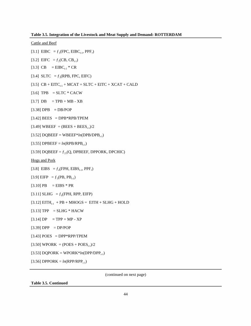
44
Table 3.5. Integration of the Livestock and Meat Supply and Demand: ROTTERDAM
Cattle and Beef
[3.1] EIBC = ƒ1(FPC, EIBCt-1, PPF,)
[3.2] EIFC = ƒ2(CB, CBt-1)
[3.3] CB = EIBCt-1 * CR
[3.4] SLTC = ƒ3(RPB, FPC, EIFC)
[3.5] CB + EITCt-1 + MCAT = SLTC + EITC + XCAT + CALD
[3.6] TPB = SLTC * CACW
[3.7] DB = TPB + MB - XB
[3.38] DPB = DB/POP
[3.42] BEES = DPB*RPB/TPEM
[3.49] WBEEF = (BEES + BEESt-1)/2
[3.52] DQBEEF = WBEEF*ln(DPB/DPBt-1)
[3.55] DPBEEF = ln(RPB/RPBt-1)
[3.59] DQBEEF = ƒ21(Q, DPBEEF, DPPORK, DPCHIC)
Hogs and Pork
[3.8] EIBS = ƒ4(FPH, EIBSt-1, PPF,)
[3.9] EIFP = ƒ5(PB, PBt-1)
[3.10] PB = EIBS * PR
[3.11] SLHG = ƒ6(FPH, RPP, EIFP)
[3.12] EITHt-1 + PB + MHOGS = EITH + SLHG + HOLD
[3.13] TPP = SLHG * HACW
[3.14] DP = TPP + MP - XP
[3.39] DPP = DP/POP
[3.43] POES = DPP*RPP/TPEM
[3.50] WPORK = (POES + POESt-1)/2
[3.53] DQPORK = WPORK*ln(DPP/DPPt-1)
[3.56] DPPORK = ln(RPP/RPPt-1)
(continued on next page)
Table 3.5. Continued

45
[3.60] DQPORK = ƒ22(Q, DPBEEF, DPPORK, DPCHIC)
Chicken and Chicken Meat
[3.15] SLCH = ƒ7(RPCH, SLCHt-1, T, PPF)
[3.16] TPCH = SLCH * CHCW
[3.17] DCH = TPCH + MCH - XCH
[3.40] DPCH = DCH/POP
[3.44] CHES = DPCH*RPCH/TPEM
[3.51] WCHIC = (CHES + CHESt-1)/2
[3.54] DQCHIC = WCHIC*ln(DPCH/DPCHt-1)
[3.57] DPCHIC = ln(RPCH/RPCHt-1)
[3.61] DQCHIC = ƒ23(Q, DPBEEF, DPPORK, DPCHIC)
Identities
[3.58] Q = DQBEEF + DQPORK + DQCHI
[3.41] TPEM = DPB*RPB + DPP*RPP + DPCH*RPCH

46
Table 3.6. Integration of the Livestock and Meat Supply and Demand: Single Equation
Cattle and Beef
[3.1] EIBC = ƒ1(FPC, EIBCt-1, PPF,)
[3.2] EIFC = ƒ2(CB, CBt-1)
[3.3] CB = EIBCt-1 * CR
[3.4] SLTC = ƒ3(RPB, FPC, EIFC)
[3.5] CB + EITCt-1 + MCAT = SLTC + EITC + XCAT + CALD
[3.6] TPB = SLTC * CACW
[3.38] DPB = DB/POP
[3.62] DPB = ƒ24(RPB, RPP, RPCH, RPI)
Hogs and Pork
[3.8] EIBS = ƒ4(FPH, EIBSt-1, PPF,)
[3.9] EIFP = ƒ5(PB, PBt-1)
[3.10] PB = EIBS * PR
[3.11] SLHG = ƒ6(FPH, RPP, EIFP)
[3.12] EITHt-1 + PB + MHOGS = EITH + SLHG + HOLD
[3.13] TPP = SLHG * HACW
[3.14] DP = TPP + MP - XP
[3.39] DPP = DP/POP
[3.63] DPP = ƒ25(RPB, RPP, RPCH, RPI)
Chicken and Chicken Meat
[3.15] SLCH = ƒ7(RPCH, SLCHt-1, T, PPF)
[3.16] TPCH = SLCH * CHCW
[3.17] DCH = TPCH + MCH - XCH
[3.40] DPCH = DCH/POP
[3.64] DPCH = ƒ26(RPB, RPP, RPCH, RPI)

47
Table 3.7. Definition of Variables for Model Section
Jointly Determined Variables
AHC = Area Harvested of Corn
AHS = Area Harvested of Sorghum
AHSB = Area Harvested of Soybean
APC = Area Planted of Corn
APS = Area Planted of Sorghum
APSB = Area Planted of Soybean
BEES = Beef Expenditure Share
CB = Calves Born
CDSB = Crush Demand for Soybean
CHES = Chicken Expenditure Share
DB = Demand for Beef
DCH = Demand for Chicken
DP = Demand for Pork
DPB = Demand Per-capita of Beef
DPCH = Demand Per-capita of Chicken
DPP = Demand Per-capita of Pork
DSM = Demand for Soymeal
EIBC = Ending Inv. of Breeding Cattle
EIBS = Ending Inventory of Breeding Sows
EIFC = Ending Inv. of Feeder Cattle
EIFP = Ending Inventory of Feeder Pigs
EITC = Ending Inv. of Total Cattle
EITH = Ending Inventory of Total Hogs
FDC = Feed Demand of Corn
FDS = Feed Demand for Sorghum
FPC = Farm Price of Cattle
FPH = Farm Price of Hogs
GCA = Grain Consuming Animals
MPI = Meat Price Index
PB = Piglets Born
(continued on next page)
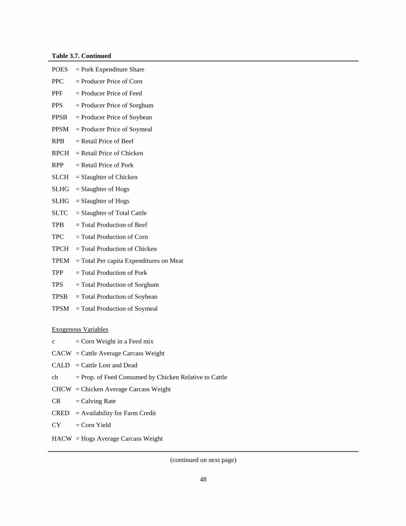
48
Table 3.7. Continued
POES = Pork Expenditure Share
PPC = Producer Price of Corn
PPF = Producer Price of Feed
PPS = Producer Price of Sorghum
PPSB = Producer Price of Soybean
PPSM = Producer Price of Soymeal
RPB = Retail Price of Beef
RPCH = Retail Price of Chicken
RPP = Retail Price of Pork
SLCH = Slaughter of Chicken
SLHG = Slaughter of Hogs
SLHG = Slaughter of Hogs
SLTC = Slaughter of Total Cattle
TPB = Total Production of Beef
TPC = Total Production of Corn
TPCH = Total Production of Chicken
TPEM = Total Per capita Expenditures on Meat
TPP = Total Production of Pork
TPS = Total Production of Sorghum
TPSB = Total Production of Soybean
TPSM = Total Production of Soymeal
Exogenous Variables
c = Corn Weight in a Feed mix
CACW = Cattle Average Carcass Weight
CALD = Cattle Lost and Dead
ch = Prop. of Feed Consumed by Chicken Relative to Cattle
CHCW = Chicken Average Carcass Weight
CR = Calving Rate
CRED = Availability for Farm Credit
CY = Corn Yield
HACW = Hogs Average Carcass Weight
(continued on next page)

49
Table 3.7. Continued
HOLD = Hogs Lost and Dead
MB = Imports of Beef
MC = Imports of Corn
MCAT = Imports of Total Cattle
MCH = Imports of Chicken
MHOGS= Imports of Total Hogs
MP = Imports of Pork
MS = Imports of Sorghum
MSB = Imports of Soybean
MSM = Imports of Soymeal
MYSB = Meal Yield of Soybean
NCDSB = Non-crush Demand for Soybean
NFDC = Non-feed Demand for Corn
NFDS = Non-feed Demand for Sorghum
p = Prop. of Feed Consumed by Hogs Relative to Cattle
Pop = Total Mexican Population
PR = Piglets Bearing Rate
RPI = Real Per capita Income
s = Sorghum Weight in a Feed mix
SBY = Soybean Yield
SEED = Input Costs in Farming
sm = Soymeal Weight in a Feed mix
SY = Sorghum Yield
T = Technological Change
XB = Exports of Beef
XCAT = Exports of Total Cattle
XCH = Exports of Chicken
XP = Exports of Pork
XS = Exports of Sorghum

50
EMPIRICAL ANALYSIS
This section presents the results of the empirical analysis performed using the model presented in the previous section.First, some data considerations are discussed. Then, the estimation procedures are reviewed and some econometricconsiderations are discussed. The meat demand model is tested for structural change and for price endogeneity. Theresults of the empirical estimation are presented and discussed. Historical simulation is then performed to evaluate andselect among the three alternative model specifications presented in the previous section. The best specification will thenbe selected for the simulation presented in the next section.
Data Sources and Considerations
As discussed earlier, reliability has been a problem for official Mexican data. Only recently, has the Mexican governmenttaken measures to develop a credible and consistent data base of the Mexican economy. The Instituto Nacional deEstadistica, Geografia e Informatica (INEGI) (National Institute of Statistics, Geography, and Information) was recentlycreated to coordinate the collection, organization, and dissemination of information in Mexico. In the past, severalagencies would collect and distribute data to only a select number of organizations. Two or more agencies wouldsometimes collect the same data with different methodologies with widely different results. Lack of consistency in theorganization of the Federal Administration has also been a problem. In the last three Federal periods (of six years each),several government ministries have been created and disappeared.
Data used for this study came mainly from the annual Mexican Presidential Report to the Congress. The report containsthe most complete data set available in Mexico. The report compiles information from all the different official Federalagencies. Data used for this analysis range from 1972 to 1991. Complete series for some variables in the conceptualmodel presented in the previous section were not available. Consequently, some modifications were made to the model.Data for information about macroeconomic variables, crop area harvested, crop prices, livestock inventories, meat andcrop production, imports and exports, production credit, and input costs were all taken from the Presidential Report. Datafor Mexican meat and livestock prices were provided by the Colegio de Posgraduados in Chapingo, Mexico. Data onsoymeal was obtained from the National Transformation Industry Association (CANACINTRA). The proportions usedto estimate the number of grain consuming animal units were taken also from several issues of Agricultural Statistics(USDA) since no equivalent information is available in Mexico. Weights used to estimate the average producer priceof feed were taken from the literature (Perez-Espejo).
Estimation Procedures
As mentioned in the background section, after the 1982 economic crisis, expenditures on meat consumption in Mexicosuffered a setback. As depicted in figure 4.1, total per capita expenditures on meat reached a high in 1982 and fell almost50% by 1991. Also, after the trade liberalization trend started in 1986 in Mexico, beef imports began to appear and percapita beef consumption jumped from 12.6 kg in 1985 to 15.7 kg in 1986. On the other hand, pork consumptiondecreased from 16.6 kg to 12.1 kg over the same period (Figure 4.2). This pattern indicates the possibility of structuralchange in meat consumption in Mexico. Several studies (Moschini and Meilke, Eales and Unnevehr, Chavas (83),Braschler, Nyankori and Miller, Garcia Vega, Tsai) test or discuss the issue of structural change in meat consumption.In most cases, parameter instability has been used to demonstrate the evidence of structural change. However, Chavas(89) affirms that the simple change in parameters over the years may not be enough to affirm that structural change hasoccurred. Chavas defines structural change as a change in the basic hypotheses used in the analysis of economicbehavior. He contends that model specification and period selection might influence the results obtained.
Given the changes in the Mexican economy that have occurred, particularly since 1982, a test for structural change inMexican meat consumption would be necessary. To avoid the problem of unique specification and period selectiondiscussed by Chavas, three specifications (AIDS, ROTTERDAM, and LINEAR) and two period selections will be usedto test for structural change in the Mexican meat consumption behavior. The selection of the two time periods was basedon the discussion in the background section. The first period (1983-91) represents the years after the 1982 economiccrisis in Mexico. The second period (1986-91) refers to the years since Mexico began the process of unilateral trade

51
liberalization. The results of the three specifications for each period will be compared to draw conclusions aboutstructural change in Mexican meat consumption patterns.
In demand systems estimation, supply is generally assumed to be perfectly elastic. In the AIDS model, prices areassumed to be fixed, this is, exogenously determined. Deaton and Muellbauer derived the AIDS model from anexpenditure function representing the PIGLOG (Price independent, generalized linearity) class of preferences. Thispermits perfect aggregation over consumers and results in representative demand functions that are correctly estimatedusing market level data. The demand functions maintain the fixed price assumption, however. Previous studies haveshown that endogeneity may be present with respect to the prices of a demand model (Wahl, Tsai). Also, when a meatdemand system is integrated into a larger supply and demand system, price endogeneity has been shown to lead toimproved demand parameter estimation results (Tsai). In this study, once the evidence of structural change has beenaccepted or rejected, a test for price endogeneity on the demand model will be performed. The test to be used (Hausmanspecification test) will be discussed later.
After endogeneity is accepted or rejected for each demand model, each demand specification will be integrated into thelivestock and feedgrain models. A sensitivity test will be performed to analyze the effects of a 20% increase in cattleexports. The magnitude and direction of the changes in the endogenous variables will then be compared. The modelspecification that tracks the historical data better and performs better in the sensitivity analysis according to standardsimulation statistics will then be used for the simulation of the effects of US-Mexico trade liberalization in the nextsection.
Econometric Considerations
In many cases, Ordinary Least Squares (OLS) is the most appropriate estimation procedure for single equation models(Pindyck and Rubinfeld). However, multiple equation models include several endogenous variables which aresimultaneously determined. Simultaneity can cause OLS parameters estimators to be inconsistent. In simultaneousequation models, endogenous variables in one equation are used as explanatory variables in other equations. Hence, theerror terms may be correlated with the endogenous variables. Consequently, OLS estimation would be both biased andinconsistent. Instrumental variables estimation is reasonable in the context of simultaneous equation models because theexogenous and predetermined variables in the model serve as excellent instrumental variables. Indirect least squares(ILS) can be used to obtain consistent parameter estimates. However, in some cases it is not possible to use ILS and, incases of overidentified equations, ILS leads to several distinct estimators.
Two Stage Least Squares (2SLS) provides a useful estimation procedure for obtaining the values of structural parametersin overidentified equations. The 2SLS estimator uses the information available from the specification of an equationsystem to obtain a unique estimate for each structural parameter.
Although 2SLS yields consistent parameter estimates when equation systems are simultaneous, as a general rule 2SLSestimates are inefficient because they apply only to a single equation within the system of equations (Pindyck andRubinfeld). The problem of lost of efficiency can be resolved by using a method of estimating system of equations inwhich parameters for all equations are determined in a single procedure. When there is no simultaneity in a system ofequations but the errors are correlated, then the Seemingly Unrelated Regression (SUR) technique may be employed.The SUR method involves generalized least-squares estimation and achieves an improvement in efficiency by takinginto explicit account the fact that cross-equation error correlation may not be zero. The natural extension of the SURestimation for a simultaneous equation model is the Three Stage Least Square technique (3SLS). The 3SLS procedureinvolves the application of generalized least-squares estimation to the system of equations, each of which has first beenestimated using 2SLS.
SUR estimation has been generally used to estimate demand systems like the AIDS and the ROTTERDAM because ofthe assumption of price exogeneity. In this study, SUR estimation will be used to test for structural change in Mexicanmeat demand. After the evidence of structural change has been accepted or rejected, the three alternative specificationswill be estimated using both SUR and 3SLS. As mentioned earlier, SUR accounts for the fact that cross-equation error

52
correlation might not be zero but does not consider simultaneity. 3SLS does consider simultaneity among equations butmay be inefficient if the prices are in fact exogenous.
The Hausman specification test (Hausman) will be performed to test for endogeneity of prices in the meat demandsystem. Consider the null hypothesis that the prices on the right-hand side of a demand system are exogenous. Underthe null hypothesis, SUR estimation is consistent and asymptotically efficient but inconsistent under the alternativehypothesis. 3SLS is consistent under both the null and the alternative hypotheses but inefficient under the nullhypothesis. This inefficiency may be relatively small, however, and the loss in efficiency may be offset by the gain insimulation performance. Accounting for endogeneity of some variables may bring more consistent parameter estimatesand may capture some information that could be lost by considering those variables as exogenous. As Tsai stated, whenthe meat demand model is combined with a livestock and feedgrain models, the parameter estimates may be improved.Both techniques SUR and 3SLS will be tested by the simulation performance once the model is fully integrated with themeat, livestock, and feedgrain sectors.
Using SUR and 3SLS, the Hausman specification test consists of determining how large the difference is between thetwo set of parameters in relation to its variance. Let b be a vector of coefficient estimates of a demand system using SUR.Let b* be a vector of coefficient estimates of the same demand system obtained using 3SLS. Let var (b) be the parametervariance-covariance matrix from the SUR estimation and var (b*) be the parameter variance-covariance matrix from the3SLS estimation. The test for misspecification is:
[4.1] m = q' M(q)-1 q,
where q=b-b*, M(q)=var(b)-var(b*), m has a chi-squared distribution with n degrees of freedom, and n is the number ofparameters in b that are directly affected by the correction for endogeneity. If m is greater than the chi-square value, thenthe null hypothesis of price exogeneity is rejected and the alternative hypothesis of endogeneity is accepted. The largerthe difference between the set of parameters (b-b*), the more likely that the alternative hypothesis of endogeneity isaccepted.
After the endogeneity hypothesis has been tested, the three demand specifications will be integrated to the livestock andfeedgrain components to simulate historical data. Simulation statistics like the root mean square and the Theil simulationstatistics will be used to evaluate which model performs better in tracking historical data.
Structural Change in Mexican Meat Consumption Behavior Table 4.1 shows the results obtained for the three demand specifications when an intercept shifter is added. A dummyvariable (equal to zero from 1972 to 1982, equal to one from 1982 to 1991) was included in every equation to captureany possible change in the behavior of meat consumption in Mexico between the two periods. Testing the hypothesisthat several coefficients are jointly equal to zero in the context of a multiple regression model can be performed by usingthe F distribution. However, when the hypothesis is that a single regression coefficient is equal to zero, the F test isreduced to a t test. Since only intercept shifters were included, the t test will be used to test for structural change in meatconsumption in Mexico.
R-Squares for the nine equations are over the 90% level except for the beef and chicken equations in the ROTTERDAMspecification (Table 4.1). Both the ROTTERDAM and the AIDS specifications showed evidence of serial correlationand were corrected for serial correlation. The resulting rho values are presented in table 4.1. The Durbin-Watson (D-W)statistic indicates the absence of serial correlation in all cases except possibly for beef on the linear specification, whichfalls into the inconclusive region. As the t-values show, out of nine estimated parameters for the 1982-91 dummy, onlyone (beef equation in the linear specification) was significant at the 10% level and none was at the 5% level.
Table 4.2 shows the results of the analysis for structural change when a different period (1986-91) is considered. Again,a dummy equal to zero from 1972 to 1985 and equal to one for the rest of the sample was included as an intercept shifter.R-Squares are similar to those from the period 1983-1991 except that they are lower for the three equations using theROTTERDAM specification. The D-W statistic values are also generally less conclusive. There is however, an

53
improvement in the number of significant parameters. Out of nine parameters estimated related to the structural changetest, five were significant at the 5% level.
The results of neither period, however, are conclusive. When the first period (1983-91) was considered, the AIDS andthe ROTTERDAM models resulted in a negative but insignificant coefficient for pork consumption and a positive butinsignificant coefficients for beef and chicken. The linear specification resulted in negative coefficients for all three typesof meats. Only the beef equation had a significant parameter at the 10% level. Using the second period (1986-91) toanalyze structural change, pork consumption in all three specifications resulted in negative and significant (5% level)coefficients. However, beef was affected negatively under the AIDS specification but positively under theROTTERDAM and the LINEAR specifications. Chicken was positively affected under the AIDS and the ROTTERDAMspecifications, but negatively under the LINEAR specification. The dummy parameter is significant for chicken in theAIDS model and for beef in the ROTTERDAM model. Hence, the results using the second period fail to demonstrateevidence of a structural change occurred in Mexican meat consumption behavior following trade liberalization. Becauselittle was found during any period or for any specification, the hypothesis of structural change in meat demand in Mexicois rejected.
Parameter Estimation for the Demand Model and Endogeneity Results
Tables 4.3, 4.4, and 4.5 show the results of model parameter estimation using 3SLS and SUR for the AIDS specification.Parameter values, the corresponding t values, and summary statistics for both 3SLS and SUR techniques are shown inTable 4.3. As discussed before, one equation (chicken) had to be dropped to avoid singularity of the variance-covariancematrix of disturbances. The parameters relative to this equation were recovered using the classical restrictions ofhomogeneity, symmetry, and adding-up.
Most of the estimated parameters are significant under both techniques (3SLS, and SUR) except for the chickenequations, where only half of the eight recovered parameters are significant. The magnitudes of those parameters underboth estimation techniques are very similar. Using the Hausman specification test, the m statistic for the AIDSspecification is -0.25. The corresponding Chi-square distribution 5% cut-off point with eight degrees of freedom is 15.51.Therefore, consistency of the SUR estimates cannot be rejected, implying that prices may be treated as exogenous whenusing the AIDS specification to estimate meat demand parameters in Mexico.
Table 4.4 provides the estimated elasticities for the AIDS model when using 3SLS estimation. The expenditure elasticityis quite large for pork while negative for chicken. Both the Marshallian and the Hicksian own price elasticities arenegative for the three types of meat. Some of the cross price effects are somewhat inconsistent with prior expectations,however. The Marshallian elasticities for pork and chicken indicate reciprocal complementarity with beef andsubstitutability between them. The Hicksian elasticities also indicate net complementarity between chicken and beef.Table 4.5 provides the resulting elasticities for the AIDS specification using the SUR estimation technique. Estimatedelasticities look very similar under the 3SLS and SUR estimation techniques. Complementarity is also present in thiscase.
Table 4.6 shows the parameters estimates obtained using the ROTTERDAM specification and the 3SLS and SURestimation techniques. R-squares and parameter significance are lower than in the AIDS specification. Of the twelveestimated and recovered parameters for each estimation technique, only two are significant at the 5% level. The similarityof the parameters under both techniques is still quite high. The m statistic of the Hausman test for the ROTTERDAMspecification is 0.71 which again implies rejection of the alternative hypothesis of inconsistency of the SUR estimates(the Chi-square distribution value at the 5% level of significance with six degrees of freedom is 12.59).
Tables 4.7 and 4.8 provide the estimated elasticities for both the 3SLS and the SUR techniques, respectively, using theROTTERDAM specification. Pork still has a large expenditure elasticity. The chicken expenditure elasticity is positive,however, in contrast to the AIDS model. Marshallian and Hicksian elasticities show complementarity problems as in theAIDS case and even beef and pork exhibit positive own-price elasticities in the Hicksian sense.

54
Table 4.9 shows the parameter estimates for the LINEAR specification using both the 3SLS and the SUR techniques.As mentioned earlier, no equation had to be dropped under this specification. R-square for the three equations in bothcases are above 90%. The D-W statistic results do not provide conclusive evidence of serial correlation in any case.Parameter significance under the LINEAR specification is better than the ROTTERDAM but not as good as the AIDSspecification. Again, the parameters are quite similar under both the 3SLS and SUR estimation. The m statistic for theHausman specification test is 1.53. The corresponding value of the Chi-square distribution at the 5% level with 15degrees of freedom is 25. Hence, the null hypothesis of consistency of the SUR estimation again cannot be rejected.
Elasticities for the LINEAR specification for both estimation techniques are provided in table 4.10 and 4.11, respectively.Pork shows again the largest income effect and chicken has a negative income effect as in the case of the AIDSspecification. Marshallian and Hicksian elasticities have the expected signs consistent with prior expectations in boththe 3SLS and SUR models except for the Hicksian elasticity for chicken on the beef equation, likely as a result of thenegative income effect for chicken. Magnitude of the elasticities for both techniques are quite similar as expected dueto the similarity of the estimated parameters.
In summary, six models were estimated: three different specifications and two estimation techniques. R-squares for theAIDS and the LINEAR specifications were over 95% in most cases. In the ROTTERDAM specification, the R-squareswere somewhat lower. The D-W statistics did not show conclusive evidence of serial correlation in any case. The bestparameter significance was found under the AIDS specification and the worst in the ROTTERDAM model. Theelasticities indicated many cases of complementarity in the AIDS and the ROTTERDAM specifications but not for theLINEAR model. Complementarity has been a common problem among researchers when estimating demand systems.The response has generally been to note the problem and to try to formulate a reasonable justification for the counter-intuitive results. In simulation, however, counter-intuitive complementarity can produce counter-intuitive results andinappropriate policy recommendations.
The chicken income elasticity was negative in the AIDS and the LINEAR specifications. A negative income elasticityfor chicken implies that Mexicans consume more chicken as income decreases. This appears to be consistent withhistorical behavior in Mexico. As discussed in the background section, as per capita income dropped following theeconomic crisis of 1982, chicken consumption increased steadily. Income elasticity for pork was shown to be larger thanthat of beef in all six models estimated. The main factors that contribute to this behavior may be prices and meatprocessing. As shown in table 2.6, pork prices have been consistently higher than those of beef. In addition, ham, bacon,and other pork derivatives are quite expensive in Mexico and only high income consumer are able to purchase themregularly.
The endogeneity test performed on the three specifications failed to reject the null hypothesis of SUR estimationconsistency. Prices for the demand system could be treated as exogenous using the SUR estimation technique whendemand estimation is performed independently. However, as discussed by Tsai, when simultaneity of meat and livestocksupply and demand is present, 3SLS has proven to provide a better performance. Therefore, 3SLS will be used toestimate the fully integrated Mexican meat, livestock, and feedgrain model.
Mexican Meat Demand Simulation
The three model specifications were integrated with the livestock supply and feedgrain supply and demand componentsto simulate historical data in Mexico. Unfortunately, the AIDS specification converged only for 3 observations and theROTTERDAM specification did not converge in simulation over the historical period. Complementarity among meatproducts within the AIDS and the ROTTERDAM specifications combined with a large expenditure elasticity for porkcould have caused the no-convergence.
The LINEAR specification was the only one to converge. Theil statistics indicate a small bias and a reasonably goodability to track historical data. The LINEAR specification for the Mexican meat demand model will then be used for asensitivity test in the next section.
The Fully Integrated Mexican Livestock, Meat, and Feedgrain Model

55
The livestock and meat supply and the feedgrain supply and demand models were integrated with the linear specificationto perform a sensitivity analysis. The original intention was to do the same with the AIDS and the ROTTERDAM modelsto compare the results. But since those models would not converge, only the linear specification was used. A change of20% in cattle exports was used to measure the magnitude and the direction of the impact on the endogenous variables.First, the resulting parameters of the fully integrated model are presented in Table 4.12. Definition of the variables isdescribed in Table 4.13.
Several modifications were made to the models as presented in Tables 3.1 and 3.2. First, data differentiating feeder frombreeding cattle inventories were not available for Mexico. Only data for cattle inventories were available. Second, theoriginal inventory equations included two lag periods for inventories and exogenous factors with one lag. However,inventory lagged two periods and lagged exogenous variables were not significant and dropped from the livestockinventory equations. The profit representation for the livestock equation, defined by farm price divided by the price offeed, was decomposed into farm prices of livestock and the producer price of feed, both deflated by the wholesale priceindex to separately capture the effect of those variables. In the feedgrain model, incomplete series were found for areaplanted. Consequently, area harvested was used to estimate supply behavior. Demand for feedgrains was estimated astotal demand because no separate data were available for feed and non-feed demand for grains. Due to the high ratesof inflation that have existed in Mexico during the last 20 years, all prices were deflated. Meat prices and per capitaincome were deflated by the consumer price index while feedgrain and livestock prices were deflated by the wholesaleprice index. Finally, lagged per capita consumption was added to each equation in the meat demand model.
Table 4.12 presents the results of the parameter estimation. Quantities in parentheses are the t-values while quantitiesin brackets represent the elasticities, ceteris paribus. Since the model is simultaneous, net effects can only be obtainedby using the analytical derived reduced form. In this section, the term elasticity will be used to indicate the gross effectbetween two variables multiplied by the ratio of their means.
Equations (4.1) to (4.8) in Table 4.12 are the equations for the cattle and beef supply and demand models. Equation (4.1)is the cattle inventory equation. The high estimated parameter for lagged ending inventory indicates that beginninginventories determine a big percentage of ending cattle inventories (eitc). The estimated results indicate that eitcincreases with an increase in farm price of cattle (fpc) and decreases if the price of feed (ppf) rises. The correspondingshort run elasticities are quite small, 0.02 for fpc and -0.01 for ppf. The long run elasticities are only slightly larger, 0.15and -0.08, respectively. This may be an indication that, because of beef price controls in Mexico, cattle producers havebeen quite unresponsive to changes in cattle prices. The low elasticity of the price of feed is not surprising because ofthe low percentage of cattle fed with feedgrains in Mexico.
The behavior of slaughter of cattle (sltc) is presented in equation (4.2) in Table 4.12. The availability of cattle representedby beginning inventories of cattle (eitct-1) has a large elasticity (7.08). That is for a one percent change in beginning cattleinventories slaughter is expected to change by seven percent. The cattle slaughter input price (fpc) has the expectednegative effect on slaughter and an elasticity equal to -0.68. The output price (retail price of beef (rpb)) has a lowelasticity of 0.10. Calves born (cb) are calculated as the product of beginning inventories of total cattle times the calvingrate (cr) (equation (4.3)). Equation (4.4) is the market clearing equation for live cattle as explained previously in chapterIII.
Total production of beef (tpb) is specified in equation (4.5) as the product of cattle slaughtered and the average cattlecarcass weight (cacw). Equation (4.6) is the market clearing equation for beef. Equation (4.7) estimates per capitaconsumption of beef (qb) by dividing total demand for beef (db) by population (pop). Finally, equation (4.8) shows theper capita beef demand relationship previously explained with only slight changes in parameters due to the inclusion oflagged per capita consumption. Long run elasticities for price of beef (rpb), price of pork (rpp), price of chicken (rpch),and per capita income (rpci) are estimated to be -0.42, 0.17, 0.16, and 0.75 respectively.
Hog and pork behavioral equations are presented in equations (4.9) to (4.15). Similar to cattle, ending inventories of totalhogs (eith) vary positively with respect to farm price of hogs (fph) and negatively with respect to price of feed (ppf).Also, lagged inventories are a strong determinant of ending inventories as shown by the estimated coefficient (0.83) and
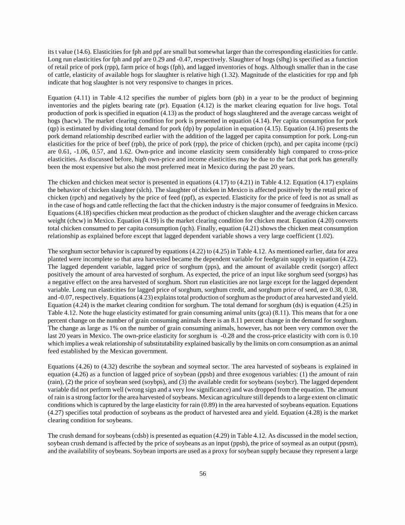
56
its t value (14.6). Elasticities for fph and ppf are small but somewhat larger than the corresponding elasticities for cattle.Long run elasticities for fph and ppf are 0.29 and -0.47, respectively. Slaughter of hogs (slhg) is specified as a functionof retail price of pork (rpp), farm price of hogs (fph), and lagged inventories of hogs. Although smaller than in the caseof cattle, elasticity of available hogs for slaughter is relative high (1.32). Magnitude of the elasticities for rpp and fphindicate that hog slaughter is not very responsive to changes in prices.
Equation (4.11) in Table 4.12 specifies the number of piglets born (pb) in a year to be the product of beginninginventories and the piglets bearing rate (pr). Equation (4.12) is the market clearing equation for live hogs. Totalproduction of pork is specified in equation (4.13) as the product of hogs slaughtered and the average carcass weight ofhogs (hacw). The market clearing condition for pork is presented in equation (4.14). Per capita consumption for pork(qp) is estimated by dividing total demand for pork (dp) by population in equation (4.15). Equation (4.16) presents thepork demand relationship described earlier with the addition of the lagged per capita consumption for pork. Long-runelasticities for the price of beef (rpb), the price of pork (rpp), the price of chicken (rpch), and per capita income (rpci)are 0.61, -1.06, 0.57, and 1.62. Own-price and income elasticity seem considerably high compared to cross-priceelasticities. As discussed before, high own-price and income elasticities may be due to the fact that pork has generallybeen the most expensive but also the most preferred meat in Mexico during the past 20 years.
The chicken and chicken meat sector is presented in equations (4.17) to (4.21) in Table 4.12. Equation (4.17) explainsthe behavior of chicken slaughter (slch). The slaughter of chicken in Mexico is affected positively by the retail price ofchicken (rpch) and negatively by the price of feed (ppf), as expected. Elasticity for the price of feed is not as small asin the case of hogs and cattle reflecting the fact that the chicken industry is the major consumer of feedgrains in Mexico.Equations (4.18) specifies chicken meat production as the product of chicken slaughter and the average chicken carcassweight (chcw) in Mexico. Equation (4.19) is the market clearing condition for chicken meat. Equation (4.20) convertstotal chicken consumed to per capita consumption (qch). Finally, equation (4.21) shows the chicken meat consumptionrelationship as explained before except that lagged dependent variable shows a very large coefficient (1.02).
The sorghum sector behavior is captured by equations (4.22) to (4.25) in Table 4.12. As mentioned earlier, data for areaplanted were incomplete so that area harvested became the dependent variable for feedgrain supply in equation (4.22).The lagged dependent variable, lagged price of sorghum (pps), and the amount of available credit (sorgcr) affectpositively the amount of area harvested of sorghum. As expected, the price of an input like sorghum seed (sorgps) hasa negative effect on the area harvested of sorghum. Short run elasticities are not large except for the lagged dependentvariable. Long run elasticities for lagged price of sorghum, sorghum credit, and sorghum price of seed, are 0.38, 0.38,and -0.07, respectively. Equations (4.23) explains total production of sorghum as the product of area harvested and yield.Equation (4.24) is the market clearing condition for sorghum. The total demand for sorghum (ds) is equation (4.25) inTable 4.12. Note the huge elasticity estimated for grain consuming animal units (gca) (8.11). This means that for a onepercent change on the number of grain consuming animals there is an 8.11 percent change in the demand for sorghum.The change as large as 1% on the number of grain consuming animals, however, has not been very common over thelast 20 years in Mexico. The own-price elasticity for sorghum is -0.28 and the cross-price elasticity with corn is 0.10which implies a weak relationship of substitutability explained basically by the limits on corn consumption as an animalfeed established by the Mexican government.
Equations (4.26) to (4.32) describe the soybean and soymeal sector. The area harvested of soybeans is explained inequation (4.26) as a function of lagged price of soybean (ppsb) and three exogenous variables: (1) the amount of rain(rain), (2) the price of soybean seed (soybps), and (3) the available credit for soybeans (soybcr). The lagged dependentvariable did not perform well (wrong sign and a very low significance) and was dropped from the equation. The amountof rain is a strong factor for the area harvested of soybeans. Mexican agriculture still depends to a large extent on climaticconditions which is captured by the large elasticity for rain (0.89) in the area harvested of soybeans equation. Equations(4.27) specifies total production of soybeans as the product of harvested area and yield. Equation (4.28) is the marketclearing condition for soybeans.
The crush demand for soybeans (cdsb) is presented as equation (4.29) in Table 4.12. As discussed in the model section,soybean crush demand is affected by the price of soybeans as an input (ppsb), the price of soymeal as an output (ppsm),and the availability of soybeans. Soybean imports are used as a proxy for soybean supply because they represent a large

57
part of the available supply of soybeans. Estimated parameters for price of soybeans and soymeal have the expected sign.The elasticity of soybean imports is larger than both price elasticities indicating that crush is more responsive to changesin available supply than to changes in prices. Total production of soymeal and the market clearing equation for soymealare specified in equations (4.30) and (4.31), respectively. The demand for soymeal is presented in equation (4.32). Theelasticity of soymeal demand with respect to grain consuming animals again is quite large (7.92). The own-price effectis not large nor significant.
The corn sector is described in equations (4.33) to (4.36) in Table 4.12. As explained in the previous section, the areaharvested of corn is specified as a function of the lagged price of corn (ppc), and some exogenous variables, includingthe price of seed corn (cornps) and available credit for corn (corncr). Although the signs are as expected, the magnitudeof the elasticities indicates that none of the variables affects the area harvested of corn strongly. Area harvested of cornhas not varied too much in the last 20 years, hence the difficulty finding significant explanatory variables. Governmentintervention via subsidies, production for subsistence, and cultural factors may be the reasons behind the stability in theamount of area harvested of corn. Total production of corn (tpc) and the market clearing condition for corn are specifiedin equations (4.34) and (4.35), respectively. In the total demand for corn (dc) (equation (4.36)) grain consuming animalunits also has a large elasticity (4.80). The price of corn and price of sorghum reflect expected signs although theirrespective elasticities are small as in the case of demand for sorghum.
Finally, equations (4.37) and (4.38) in Table 4.12 show the calculations used to obtain the number of grain consuminganimal units (gca) and the average producer price of feed (ppf). The number of grain consuming animals, as discussedin the previous section, is an aggregated of the inventories of cattle and hogs and the number of chickens slaughteredduring each period. The aggregation factors (mcow, pork, and chi) indicate the dry-weight quantity of a feed consumedby an animal during a base period and were obtained from several issues of the USDA agricultural statistical yearbook.Although corn is not consumed as an animal feed in the same proportion as sorghum, people interviewed stated that witha lower price, corn would substitute sorghum in any feed mix.
Model Validation
Validation of the structural model was conducted through historical simulation. Root mean squared percentage error(RMS% error), Theil forecast error statistics, and sensitive analysis were used to evaluate the performance of the model.These results are shown on Tables 4.14 and 4.15.
The RMS% error is a measure of the deviation of the simulated variable from its actual time path in percentage terms.Low RMS% errors are one desirable measure of simulation fit (Pindyck and Rubinfeld). Another useful simulationstatistic applied to the evaluation of historical simulations is Theil's inequality coefficient (U). Low values of U representa good performance of the model. When U=0, then the model has a perfect fit while if U=1 the performance of the modelis as bad as it possibly could be. Theil's inequality coefficient can be decomposed in three proportions: Um, Us, and Uc
called the bias, the variance, and the covariance proportions, respectively. Um is an indication of systematic error. Itmeasures the extent to which the average values of the simulated and actual series deviate from each other. The varianceproportion Us indicates the ability of the model to replicate the degree of variability in the variable of interest. A largeUs indicates that the actual series has fluctuated considerably while the simulated series show little fluctuation or viceversa. The last measure (Uc) indicates unsystematic error which is the remaining error after deviations from averagevalues have been accounted for. Theil's inequality coefficient can also be decomposed into three other components: Um,Ur, and Ud. The first term (Um) is as described before while the second and third are called the regression proportion anddisturbance proportion. These statistics are also presented in Table 4.14. The RMS% error looks relatively small exceptfor those variables representing prices. This is to be expected since the variation in prices in the model is the result ofthe variation over a number of supply and demand variables. None of the endogenous variables show a systematic error(bias) but the same tendency for prices to vary is shown in the corresponding variance and covariance proportions andthe regression and disturbance proportions.
Table 4.15 provides the dynamic multipliers and the dynamic elasticities for selected variables calculated after anincrease of 20% on cattle exports was simulated for the year 1972. The multipliers indicate that the model is stablebecause all the variables return to equilibrium and the direction of the changes is expected. Cattle slaughter, for example,
58
is reduced in the first period as expected due to the increase in cattle exports. The magnitude of the multipliers, however,is small which means that a 20% change in cattle exports does not impact substantially the endogenous variables of themodel.
Dynamic elasticities represent a relative measure of the impact of a change in an exogenous variable. Long run multiplierfor beef, for example, was not large but the elasticity for beef relative to a change of 20% in cattle exports (1.58) is thelargest among the variables analyzed.
Summary
This section has presented the results of the empirical estimation performed on the Mexican livestock, meat, andfeedgrain model developed in the previous section. Data issues were addressed first. Reliability has been a problem forofficial Mexican data. Estimation procedures were considered after. Structural change and endogeneity of the prices inthe demand model were discussed. Then, econometric considerations were presented. The differences among severalestimation techniques like the OLS, ILS, 2SLS, SUR, and 3SLS were discussed. Three alternative model specifications(AIDS, ROTTERDAM, and LINEAR) for the Mexican meat demand were used to test for structural change. The resultsobtained did not show strong evidence that a structural change has occurred in the Mexican meat demand behavior dueto the 1982 economic crisis or to the trade liberalization that started in 1986.
Parameters for the three model specifications were estimated using both SUR and 3SLS. Complementarity problemsamong meat products were found under the AIDS and the ROTTERDAM specifications. The income and expenditureelasticity for pork was found to be relatively large (over 1). Income elasticity in the LINEAR specification andexpenditure elasticity in the AIDS specification for chicken was negative. The Mexican meat demand model was alsotested for price endogeneity using the Hausman specification test. The results of the Hausman test indicate that theparameters obtained by using SUR estimation are consistent and prices in the Mexican meat demand model may treatedas exogenous when the demand model is estimated independently. However, when estimation of livestock and meatsupply and demand is required, 3SLS estimation technique is encouraged.
The three alternative model specifications for meat demand were then integrated to the livestock and feedgraincomponents of the model. A failed attempt was made to simulate the AIDS and the ROTTERDAM specifications.Unfortunately, neither of the two converged for simulation due possibly to the existence of complementarities amongmeat products and the large income elasticity for pork. The LINEAR specification was then used to estimate theparameters of the integrated Mexican livestock, meat, and feedgrain model.
Estimated parameters for the Mexican livestock, meat, and feedgrain model were presented. Summary statistics showeda good estimation performance of the model. Among the principal results drawn from the empirical estimation are thefollowing:
1. Cattle inventories response to changes in cattle and feed prices is very small which may indicate that, due to meatprice controls in Mexico, farmers are quite unresponsive to changes in cattle prices.
2. Slaughter of cattle is highly determined by cattle supply, although cattle and beef prices affect negatively andpositively, respectively, the amount of cattle slaughter.
3. Hog inventories responses to hog and feed prices are somewhat higher than the corresponding responses for cattle.Hog slaughter is not highly affected by hog and pork prices but by available hog supply.
4. Per capita consumption of beef and pork are directly affected by changes on per capita income while the effect onchicken per capita consumption is negative.
5. Changes on feed prices seem not to affect significantly the amount of area harvested of the feed crops. Guaranteedprices and the Mexican government trade policy have caused the low response of farmers to changes on feed prices.
59
After discussing every component of the model, the model was validated using historical simulation. Simulation statisticslike the RMS% error and the Theil's statistics showed an overall good performance for all the endogenous variables,except for prices. This variation was expected, however, because the variation in prices in the model is the result of thevariation over a number of supply and demand variables. Dynamic multipliers and dynamic elasticities were alsopresented. The multipliers and elasticities indicate that the model is stable because all the variables return to equilibriumafter a shock and the direction of the changes is as expected.
Table 4.1. Mexico: Structural Change Analysis for Meat Demand (Period 1983-91)
LA/AIDS MODEL
Beef Pork Chicken
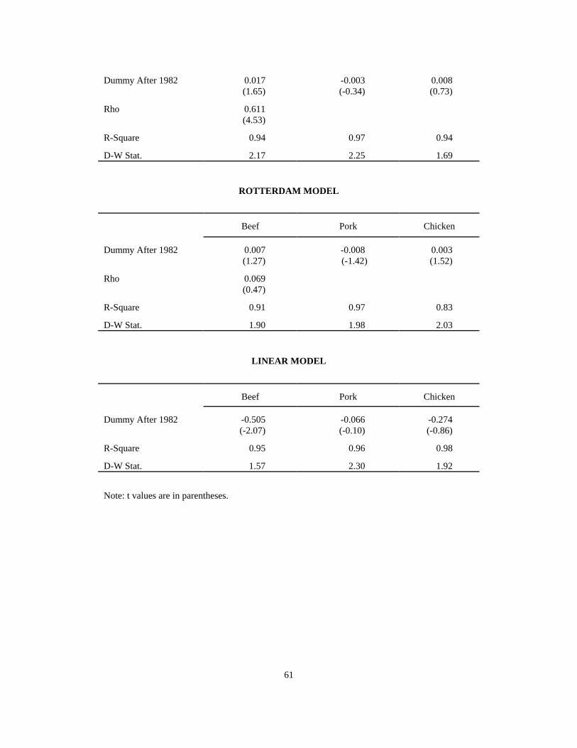
61
Dummy After 1982 0.017 (1.65)
-0.003 (-0.34)
0.008 (0.73)
Rho 0.611 (4.53)
R-Square 0.94 0.97 0.94
D-W Stat. 2.17 2.25 1.69
ROTTERDAM MODEL
Beef Pork Chicken
Dummy After 1982 0.007 (1.27)
-0.008 (-1.42)
0.003 (1.52)
Rho 0.069 (0.47)
R-Square 0.91 0.97 0.83
D-W Stat. 1.90 1.98 2.03
LINEAR MODEL
Beef Pork Chicken
Dummy After 1982 -0.505 (-2.07)
-0.066 (-0.10)
-0.274 (-0.86)
R-Square 0.95 0.96 0.98
D-W Stat. 1.57 2.30 1.92
Note: t values are in parentheses.

62
Table 4.2. Mexico: Structural Change Analysis for Meat Demand (Period 1986-91)
LA/AIDS MODEL
Beef Pork Chicken
Dummy for 1986 to1991
-0.003 (-0.27)
-0.076 (-3.72)
0.057 (6.13)
Rho 0.360 (2.39)
R-Square 0.96 0.98 0.88
D-W Stat. 2.46 1.74 1.47
ROTTERDAM MODEL
Beef Pork Chicken
Dummy for 1986 to1991
0.018 (2.57)
-0.018 (-2.41)
0.003 (1.60)
Rho 0.170 (0.94)
R-Square 0.81 0.93 0.82
D-W Stat. 1.91 1.87 1.47
LINEAR MODEL
Beef Pork Chicken
Dummy for 1986 to1991
0.076 (0.23)
-3.782 (-4.74)
-0.632 (-1.21)
R-Square 0.94 0.98 0.98
D-W Stat. 1.71 1.51 1.58
Note: t values are in parentheses.
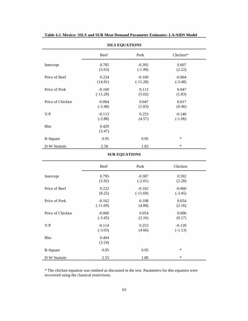
63
Table 4.3. Mexico: 3SLS and SUR Meat Demand Parameter Estimates: LA/AIDS Model
3SLS EQUATIONS
Beef Pork Chicken*
Intercept 0.785 (5.63)
-0.392 (-1.99)
0.607 (2.22)
Price of Beef 0.224 (14.81)
-0.160 (-11.28)
-0.064 (-3.48)
Price of Pork -0.160 (-11.28)
0.113 (5.02)
0.047 (1.83)
Price of Chicken -0.064 (-3.48)
0.047 (1.83)
0.017 (0.46)
Y/P -0.113 (-2.88)
0.253 (4.57)
-0.140 (-1.06)
Rho 0.429 (3.47)
R-Square 0.95 0.95 *
D-W Statistic 2.58 1.83 *
SUR EQUATIONS
Beef Pork Chicken
Intercept 0.795 (5.92)
-0.387 (-2.01)
0.592 (2.28)
Price of Beef 0.222 (8.25)
-0.162 (-11.69)
-0.060 (-3.45)
Price of Pork -0.162 (-11.69)
0.108 (4.88)
0.054 (2.16)
Price of Chicken -0.060 (-3.45)
0.054 (2.16)
0.006 (0.17)
Y/P -0.114 (-3.03)
0.253 (4.66)
-0.139 (-1.13)
Rho 0.404 (3.24)
R-Square 0.95 0.95 *
D-W Statistic 2.55 1.80 *
* The chicken equation was omitted as discussed in the text. Parameters for this equation wererecovered using the classical restrictions.

64
Table 4.4. Mexico: 3SLS Meat Demand Elasticities: LA/AIDS Model*
Expenditure Elasticities
Beef Pork Chicken
0.732(18.75)
1.546(27.91)
-0.190(-2.48)
Marshallian Elasticities
Beef Pork Chicken
Beef-0.353(-6.44)
-0.258(-6.70)
-0.121(-2.73)
Pork-0.574
(-14.92)-1.009
(-13.69)0.037(5.52)
Chicken-0.044(-0.27)
0.949(4.29)
-0.716(-2.21)
Hicksian Elasticities
Beef Pork Chicken
Beef -0.046(-1.21)
0.081(2.39)
-0.035(-0.79)
Pork 0.073(2.39)
-0.293(-6.04)
0.220(3.95)
Chicken -0.123(-0.79)
0.861(3.95)
-0.738(-2.35)
* t values are in parentheses.

65
Table 4.5. Mexico: SUR Meat Demand Elasticities: LA/AIDS Model*
Expenditure Elasticities
Beef Pork Chicken
0.728(19.31)
1.546(28.51)
-0.178(-2.41)
Marshallian Elasticities
Beef Pork Chicken
Beef -0.356(-6.64)
-0.261(-6.96)
-0.111(-2.66)
Pork -0.579(-15.38)
-1.020(-14.01)
0.052(7.94)
Chicken -0.015(-0.10)
1.003(4.68)
-0.810(-2.51)
Hicksian Elasticities
Beef Pork Chicken
Beef -0.051(-1.34)
0.076(2.30)
-0.025(-0.61)
Pork 0.069(2.30)
-0.304(-6.26)
0.235(4.35)
Chicken -0.089(-0.61)
0.921(4.35)
-0.831(-2.65)
* t values are in parentheses

66
Table 4.6. Mexico: 3SLS and SUR Meat Demand Parameter Estimates: ROTTERDAM Model
3SLS EQUATIONS
Beef Pork Chicken*
Price of Beef 0.003(0.11)
-0.022(-0.80)
0.019(1.16)
Price of Pork -0.22(-0.80)
0.035(1.03)
-0.013(-0.67)
Price of Chicken 0.019(1.16)
-0.013(-0.67)
-0.006(-0.32)
Q 0.289(3.28)
0.618(6.54)
0.093(1.48)
Rho 0.097(0.52)
R-Square 0.71 0.89 *
D-W Statistic 1.91 1.85 *
SUR EQUATIONS
Beef Pork Chicken
Price of Beef 0.004(0.15)
-0.026(-0.95)
0.021(1.40)
Price of Pork -0.026(-0.95)
0.042(1.31)
-0.016(-0.94)
Price of Chicken 0.021(1.40)
-0.016(-0.94)
-0.005(-0.30)
Q 0.302(3.36)
0.599(6.33)
0.099(1.59)
Rho 0.127(0.72)
R-Square 0.71 0.89 *
D-W Statistic 1.92 1.83 *
* The chicken equation was omitted as discussed in the text. Parameters for this equation wererecovered using the classical restrictions.

67
Table 4.7. Mexico: 3SLS Meat Demand Elasticities: ROTTERDAM Model*
Expenditure Elasticities
Beef Pork Chicken
0.690(3.27)
1.335(6.53)
0.690(0.54)
Marshallian Elasticities
Beef Pork Chicken
Beef-0.281(-4.38)
-0.735(-11.3)
0.018(0.47)
Pork-0.309(-4.38)
-0.543(-7.45)
-0.051(-1.24)
Chicken-0.869(-5.24)
-2.532(-15.7)
-0.143(-0.90)
Hicksian Elasticities
Beef Pork Chicken
Beef -0.008(-0.07)
-0.052(-0.42)
0.044(0.72)
Pork -0.047(-0.47)
0.075(0.62)
-0.027(-0.45)
Chicken 0.158(0.46)
-0.108(-0.26)
-0.050(-0.31)
* t values are in parentheses.

68
Table 4.8. Mexico: SUR Meat Demand Elasticities: ROTTERDAM Model*
Expenditure Elasticities
Beef Pork Chicken
0.720(3.36)
1.294(6.32)
0.842(0.57)
Marshallian Elasticities
Beef Pork Chicken
Beef -0.292(-4.51)
-0.723(-11.3)
0.023(0.63)
Pork -0.328(-5.67)
-0.509(-7.36)
-0.060(-1.61)
Chicken -0.890(-6.85)
-2.488(-16.9)
-0.143(-1.01)
Hicksian Elasticities
Beef Pork Chicken
Beef 0.010(0.09)
-0.061(-0.49)
0.051(0.83)
Pork -0.055(-0.55)
0.090(0.77)
-0.035(-0.60)
Chicken 0.181(0.52)
-0.137(-0.34)
-0.044(-0.31)
* t values are in parentheses.

69
Table 4.9. 3SLS and SUR Meat Demand Parameter Estimates: LINEAR Model
3SLS EQUATIONS
Beef Pork Chicken*
Intercept 4.297(1.62)
-5.345(-0.98)
2.876(1.86)
Price of Beef -0.063(-6.02)
0.019(1.80)
0.044(2.05)
Price of Pork 0.040(1.61)
-0.071(-3.83)
0.057(1.46)
Price of Chicken 0.005(0.50)
0.010(1.58)
-0.038(-3.07)
Per capita Income 0.164(3.26)
0.209(2.48)
-0.036(-1.56)
R-Square 0.94 0.96 0.98
D-W Statistic 1.82 2.44 1.68
SUR EQUATIONS
Beef Pork Chicken
Intercept 4.492(1.73)
-5.266(-0.97)
2.957(1.92)
Price of Beef -0.061(-6.02)
0.019(1.82)
0.042(1.99)
Price of Pork 0.038(1.57)
-0.071(-3.86)
0.057(1.47)
Price of Chicken 0.005(0.52)
0.010(1.57)
-0.039(-3.17)
Per capita Income 0.151(3.12)
0.211(2.53)
-0.038(-1.62)
R-Square 0.93 0.96 0.98
D-W Statistic 1.71 2.49 1.69
* The chicken equation was not omitted in this case.

70
Table 4.10. Mexico: 3SLS Meat Demand Elasticities: LINEAR Model*
Income Elasticities
Beef Pork Chicken
0.698(3.26)
0.879(2.48)
-0.334(-1.56)
Marshallian Elasticities
Beef Pork Chicken
Beef-0.418(-6.02)
0.145(1.80)
0.180(2.05)
Pork0.267(1.61)
-0.542(-3.83)
0.229(1.46)
Chicken0.072(0.50)
0.164(1.58)
-0.335(-3.07)
Hicksian Elasticities
Beef Pork Chicken
Beef -0.126(-1.10)
0.468(4.09)
-0.262(-1.53)
Pork 0.635(2.62)
-0.135(-0.65)
0.332(1.00)
Chicken -0.069(-0.54)
0.009(0.08)
-0.375(-2.65)
* t values are in parentheses.

71
Table 4.11. Mexico: SUR Meat Demand Elasticities: LINEAR Model*
Income Elasticities
Beef Pork Chicken
0.642(3.12)
0.888(2.53)
-0.346(-1.62)
Marshallian Elasticities
Beef Pork Chicken
Beef -0.411(-6.02)
0.147(1.82)
0.171(1.99)
Pork 0.253(1.57)
-0.542(-3.86)
0.230(1.47)
Chicken 0.073(0.52)
0.162(1.57)
-0.342(-3.17)
Hicksian Elasticities
Beef Pork Chicken
Beef -0.142(-1.29)
0.444(4.04)
0.247(1.49)
Pork 0.626(2.63)
-0.131(-0.64)
0.335(1.02)
Chicken -0.072(-0.57)
0.002(0.02)
-0.3.83(-2.72)
* t values are in parentheses.
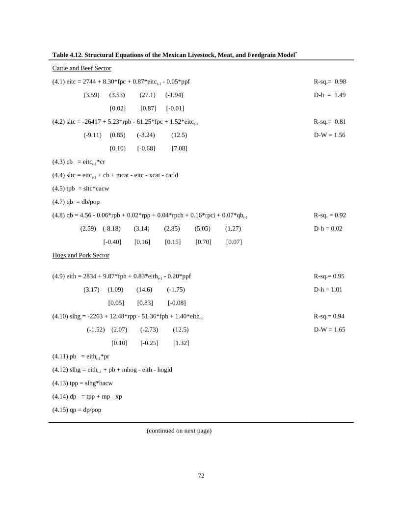
72
Table 4.12. Structural Equations of the Mexican Livestock, Meat, and Feedgrain Model*
Cattle and Beef Sector
(4.1) eitc = 2744 + 8.30*fpc + 0.87*eitct-1 - 0.05*ppf R-sq.= 0.98
(3.59) (3.53) (27.1) (-1.94) D-h = 1.49
[0.02] [0.87] [-0.01]
(4.2) sltc = -26417 + 5.23*rpb - 61.25*fpc + 1.52*eitct-1 R-sq.= 0.81
(-9.11) (0.85) (-3.24) (12.5) D-W = 1.56
[0.10] [-0.68] [7.08]
(4.3) cb = eitct-1*cr
(4.4) sltc = eitct-1 + cb + mcat - eitc - xcat - catld
(4.5) tpb = sltc*cacw
(4.7) qb = db/pop
(4.8) qb = 4.56 - 0.06*rpb + 0.02*rpp + 0.04*rpch + 0.16*rpci + 0.07*qbt-1 R-sq. = 0.92
(2.59) (-8.18) (3.14) (2.85) (5.05) (1.27) D-h = 0.02
[-0.40] [0.16] [0.15] [0.70] [0.07]
Hogs and Pork Sector
(4.9) eith = 2834 + 9.87*fph + 0.83*eitht-1 - 0.20*ppf R-sq.= 0.95
(3.17) (1.09) (14.6) (-1.75) D-h = 1.01
[0.05] [0.83] [-0.08]
(4.10) slhg = -2263 + 12.48*rpp - 51.36*fph + 1.40*eitht-1 R-sq.= 0.94
(-1.52) (2.07) (-2.73) (12.5) D-W = 1.65
[0.10] [-0.25] [1.32]
(4.11) pb = eitht-1*pr
(4.12) slhg = eitht-1 + pb + mhog - eith - hogld
(4.13) tpp = slhg*hacw
(4.14) dp = tpp + mp - xp
(4.15) qp = dp/pop
(continued on next page)

73
Table 4.12. Continued
(4.16) qp =-3.63 + 0.04*rpb - 0.06*rpp + 0.06*rpch + 0.16*rpci + 0.59*qpt-1 R-sq.= 0.95
(-1.03) (2.34) (-4.92) (2.43) (2.91) (10.9) D-h = 0.02
[0.25] [-0.43] [0.23] [0.66] [0.60]
Chicken and Chicken Meat Sector
(4.17) slch = 274 + 18.93*rpch + 0.98*slcht-1 - 0.21*ppf R-sq. = 0.97
(0.37) (2.64) (16.6) (-2.75) D-h = 0.92
[0.38] [0.94] [-0.38]
(4.18) tpch = slch*chcw
(4.19) dch = tpch + mch - xch
(4.20) qch = dch/pop
(4.21) qch =2.76 + .003*rpb + 0.01*rpp - 0.04*rpch - 0.03*rpci + 1.02*qcht-1 R-sq. = 0.98
(2.34) (0.37) (1.64) (-3.91) (-1.60) (17.1) D-h = 0.18
[0.04] [0.12] [-0.31] [-0.26] [0.99]
Sorghum Sector
(4.22) ahs = 167 + 0.71*ahst-1 + 0.05*(pps)t-1 - .001*sorgps + .0007*sorgcr R-sq. = 0.92
(1.12) (10.5) (1.43) (-0.52) (4.32) D-h = 0.63
[0.71] [0.11] [-0.02] [0.11]
(4.23) tps = ahs*sy
(4.24) ds = tps + ms - xs
(4.25) ds = -41904 + 2.08*gca - 0.54*(pps) + 0.14*(ppc) R-sq. = 0.96
(-14.5) (17.4) (-3.69) (0.96) D-W = 1.84
[8.11] [-0.28] [0.10]
Soybean and Soymeal Sector
(4.26) ahsb = -13.3 + .003*(ppsb)t-1+ + .0 1*rain - .004*soybps + .001*soybcr R-sq. = 0.96
(-0.35) (1.04) (10.3) (-3.36) (12.4) D-W = 1.92
[ -0.09] [0.89] [-0.43] [0.32]
(continued on next page)

74
Table 4.12. Continued
(4.27) tpsb = ahsb*sby
(4.28) cdsb = tpsb + msb
(4.29) cdsb = 627 + 0.04*(ppsm) - 0.07*(ppsb) + 1.26*msb R-sq. = 0.97
(4.96) (2.51) (-3.17) (27.7) D-W = 2.07
[0.20] [-0.41] [0.68]
(4.30) tpsm = cdsb*mysb
(4.31) dsm = tpsm + msm
(4.32) dsm = -7195 + 0.34*gca - .006*(ppsm) + 0.28*dsmt-1 R-sq. = 0.87
(-4.52) (5.08) (-0.43) (2.86) D-h = 0.77
[7.92] [-0.04] [0.27]
Corn Sector
(4.33) ahc = 7578 + 0.07*(ppc)t-1 - .026*sorgps + .0009*sorgcr R-sq. = 0.79
(15.2) (0.66) (-2.80) (4.37) D-W = 1.88
[0.05] [-0.09] [0.08]
(4.34) tpc = ahc*cy
(4.35) dc = tpc + mc - xc
(4.36) dc = -49086 + 2.68*gca - 0.61*(ppc) + 0.29*(pps) R-sq. = 0.93
(-6.60) (9.44) (-3.23) (0.96) D-W = 2.31
[4.80] [-0.19] [0.07]
Identities
(4.37) gca = eitc + eith*(hog/mcow) + slch*(chi/mcow)
(4.38) ppf = .4*(pps) + .4*(ppc) + .2*(ppsm)
* t values are in parentheses and gross effect elasticities are in brackets.
Table 4.13. Definition of Variables for Empirical Analysis Section

75
Jointly Determined Variables
ahc= Area Harvested of Corn
ahs = Area Harvested of Sorghum
ahs = Area Harvested of Soybean
cb = Calves Born
cdsb = Crush Demand for Soybean
db = Demand for Beef
dch = Demand for Chicken
dp = Demand for Pork
ds = Demand for Sorghum
dsm = Demand for Soymeal
eitc = Ending Inventories of Total Cattle
eith = Ending Inventory of Total Hogs
fpc = Farm Price of Cattle
fph = Farm Price of Hogs
gca = Grain Consuming Animal Units
pb = Piglets Born
ppc = Producer Price of Corn
ppf = Producer Price of Feed
pps = Producer Price of Sorghum
ppsb = Producer Price of Soybean
ppsm = Producer Price of Soymeal
qb = Per Capita Consumption of Beef
qch = Per Capita Consumption of Chicken
qp = Per Capita Consumption of Pork
rpb = Retail Price of Beef
rpch = Retail Price of Chicken
(continued on next page)
Table 4.13. Continued

76
rpp = Retail Price of Pork
slch = Slaughter of Chicken
slhg = Slaughter of Hogs
sltc = Slaughter of Cattle
tpb = Total Production of Beef
tpc = Total Production of Corn
tpch = Total Production of Chicken
tpp = Total Production of Pork
tps = Total Production of Sorghum
tpsb = Total Production of Soybean
tpsm = Total Production of Soymeal
Exogenous Variables
cacw = Cattle Average Carcass Weight
catld = Cattle Lost and Dead
chcw = Chicken Average Carcass Weight
chi = Average Feed Consumed by a Chicken in a Year
corncr = Credit Availability for Corn
cornps = Price of Corn Seed
cr = Calving Rate
cy = Corn Yield
hacw = Hogs Average Carcass Weight
hog = Average Feed Consumed by a Hog in a Year
hogld = Hogs Lost and Dead
mb = Imports of Beef
mc = Imports of Corn
mcat = Imports of Cattle
(continued on next page)
Table 4.13. Continued

77
mch = Imports of Chicken
mcow = Average Feed Consumed by a Milk Cow in a Year
mhog = Imports of Hogs
mp = Imports of Pork
ms = Imports of Sorghum
msb = Imports of Soybean
msm = Imports of Soymeal
mysb = Meal Yield of Soybean
pop = Total Mexican Population
pr = Piglets Bearing Rate
rain = Rainfall
rpci = Real Per capita Income
sby = Soybean Yield
sorgcr = Credit Availability for Sorghum
sorgps = Price of Sorghum Seed
soybcr = Credit Availability for Soybean
soybps = Price of Soybean Seed
sy = Sorghum Yield
xb = Exports of Beef
xc = Exports of Corn
xcat = Exports of Total Cattle
xch = Exports of Chicken
xp = Exports of Pork
xs = Exports of Sorghum
Table 4.14. Model Simulation Validation Statistics
MSE Decomposition Proportions

78
VariableBias(UM)
Reg(UR)
Dist(UD)
Var(US)
Covar(UC)
RMS%Error Theil's U
EITC 0.000 0.121 0.879 0.040 0.960 0.895 0.004
FPC 0.000 0.377 0.623 0.002 0.998 15.490 0.073
EITH 0.002 0.043 0.955 0.039 0.959 9.861 0.047
FPH 0.000 0.956 0.043 0.627 0.373 82.274 0.352
TPCH 0.126 0.493 0.380 0.398 0.475 15.506 0.065
AHS 0.042 0.002 0.956 0.018 0.940 5.585 0.027
PPS 0.036 0.616 0.348 0.471 0.493 35.989 0.202
AHSB 0.000 0.004 0.996 0.025 0.975 21.165 0.062
PPSB 0.042 0.699 0.259 0.134 0.824 128.95 0.672
PPSM 0.036 0.917 0.048 0.435 0.529 244.51 0.860
AHC 0.002 0.024 0.975 0.014 0.985 4.335 0.020
PPC 0.000 0.196 0.804 0.108 0.892 32.981 0.116
CB 0.015 0.000 0.985 0.001 0.984 0.819 0.004
PB 0.016 0.108 0.876 0.000 0.984 8.829 0.042
SLTC 0.006 0.142 0.852 0.034 0.960 7.126 0.033
TPB 0.006 0.127 0.867 0.034 0.961 7.126 0.033
SLHG 0.010 0.205 0.786 0.018 0.972 18.779 0.089
TPP 0.011 0.176 0.813 0.013 0.976 18.779 0.089
TPS 0.038 0.000 0.962 0.021 0.941 5.585 0.028
DS 0.038 0.146 0.817 0.196 0.767 4.472 0.021
TPSB 0.000 0.001 0.999 0.028 0.972 21.165 0.061
CDSB 0.000 0.006 0.994 0.021 0.979 7.410 0.026
TPSM 0.000 0.008 0.991 0.028 0.972 7.410 0.028
DSM 0.000 0.010 0.990 0.027 0.972 6.758 0.025
TPC 0.004 0.001 0.995 0.018 0.978 4.335 0.021
TDC 0.004 0.008 0.988 0.026 0.970 3.738 0.017
(continued on next page)
Table 4.14. Continued
MSE Decomposition Proportions

79
VariableBias(UM)
Reg(UR)
Dist(UD)
Var(US)
Covar(UC)
RMS%Error Theil's U
GCA 0.020 0.017 0.963 0.000 0.980 0.822 0.004
SLCH 0.111 0.512 0.377 0.404 0.485 15.506 0.067
PPF 0.006 0.974 0.021 0.768 0.226 85.343 0.365
RPB 0.000 0.945 0.054 0.602 0.398 48.010 0.225
RPP 0.000 0.952 0.048 0.621 0.379 88.349 0.358
RPCH 0.004 0.887 0.109 0.539 0.457 44.132 0.207
QBEEF 0.004 0.363 0.633 0.130 0.866 7.222 0.034
QPORK 0.009 0.237 0.754 0.031 0.960 18.570 0.090
QCHIC 0.088 0.537 0.375 0.402 0.509 15.176 0.066
DB 0.006 0.098 0.896 0.024 0.971 7.222 0.033
DP 0.011 0.181 0.808 0.014 0.975 18.570 0.088
DCH 0.126 0.486 0.388 0.396 0.478 15.176 0.063

80
Table 4.15. Dynamic Multipliers and Dynamic Elasticities for Selected Variables From a20% Increase in Mexican Cattle Exports
DYNAMIC MULTIPLIERS
Period EITC SLTC FPC RPB GCA PPF DS DSM
1 0.1123 -1.122 0.0301 0.1309 0.1531 2.5460 0.0000 0.0000
2 0.1105 0.0405 0.0025 0.0014 0.0764 0.3467 0.1158 0.0206
3 0.0673 0.0693 0.0019 0.0029 0.0527 0.8977 0.1123 0.0002
4 0.0785 0.0112 0.0021 0.0072 0.0225 -0.037 0.0833 0.0086
5 0.0536 0.0514 0.0010 -0.0005 0.0263 0.4770 0.0585 -0.001
6 0.0600 0.0120 0.0015 0.0039 0.0126 -0.014 0.0437 0.0043
7 0.0469 0.0341 0.0009 0.0003 0.0150 0.2699 0.0269 -0.0005
8 0.0495 0.0142 0.0011 0.0024 0.0088 0.0224 0.0266 0.0023
9 0.0388 0.0292 0.0008 0.0003 0.0131 0.2199 0.0154 -0.000
10 0.0380 0.0154 0.0008 0.0016 0.0083 0.0622 0.0203 0.0000
Long Run
Multiplier 0.62 -0.86 0.04 0.15 0.38 4.73 0.48 0.03
DYNAMIC ELASTICITIES
Period EITC SLTC FPC RPB GCA PPF DS DSM
1 0.0055 -0.3203 0.6695 1.3926 0.0066 0.4974 0.0000 0.0000
2 0.0049 0.0105 0.0521 0.0135 0.0033 0.0539 0.0341 0.0360
3 0.0030 0.0172 0.0336 0.0304 0.0022 0.1455 0.0310 0.0003
4 0.0035 0.0027 0.0432 0.0775 0.0009 -0.005 0.0195 0.0182
5 0.0023 0.0118 0.0210 -0.006 0.0011 0.0749 0.0140 -0.002
6 0.0026 0.0026 0.0277 0.0439 0.0005 -0.002 0.0097 0.0045
7 0.0021 0.0073 0.0187 0.0031 0.0006 0.0537 0.0062 -0.001
8 0.0021 0.0028 0.0201 0.0218 0.0003 0.0046 0.0064 0.0021
9 0.0016 0.0053 0.0137 0.0030 0.0005 0.0406 0.0031 -0.000
10 0.0016 0.0026 0.0131 0.0167 0.0003 0.0011 0.0032 0.0000
Long Run
Elasticity 0.03 -0.26 0.90 1.58 0.02 0.86 0.12 0.00
SIMULATION ANALYSIS
81
This section presents the results of using the Mexican livestock, meat, and feedgrain model and empirical estimates aspresented in the previous model and empirical analysis sections to analyze the effects of the unilateral liberalization ofMexican trade which began in the mid-1980s on the Mexican livestock, meat, and feedgrain sectors. Because a complete,consistent series of data for those sectors is not yet available for the period since NAFTA took effect in January of 1994,this analysis considers only the pre-NAFTA period of Mexican unilateral liberalization. The results, however, shouldprovide important insights into the effects of liberalization under NAFTA for the Mexican livestock, meat, and feedgrainsectors. In order to isolate the specific effects of liberalization of trade in each of those sectors as well as the aggregateoverall effects of liberalization on all sectors, the results of 5 different simulation scenarios will be considered:
! Liberalization of only cattle exports from Mexico;! Liberalization of only cattle imports by Mexico;! Liberalization of only meat imports by Mexico;! Liberalization of only feed imports by Mexico; and,! Liberalization of exports and imports of cattle, meat, and feed simultaneously.
Trade liberalization involves the elimination of tariffs and other trade barriers to facilitate trade. Whether tradesubsequently grows, however, depends on the pre-liberalization level of protection and changes in the economicconditions in the trading countries. That is, the lowering of tariffs will have little impact if the tariffs are low to begin withor if economic conditions in the trading countries change. Thus, while lower tariffs can boost trade, an economicdownturn in the importing country can reduce demand and offset the import effects of liberalization. In many ways, tradeliberalization largely opens the door of a country like Mexico to increased export and import opportunities. The rate ofeconomic growth in that country, however, will have a significant effect on the extent of the growth in trade as a resultof liberalization. Consequently, this section also reports the analysis of the effects of changes in Mexican per capitaincomes during the period of unilateral liberalization on Mexican exports and imports of livestock, meat, and feedgrains.
Mexican Unilateral Trade Liberalization Simulations
The Mexican government began the process of opening its markets to international trade in 1986 (see background sectionfor a detailed discussion). This process led to rapid growth in Mexican trade in livestock, meat, and grains. Cattle exportsgrew particularly rapidly (Fig. 5.1). Cattle imports also increased after 1987 although to considerably less extent thanwas the case for cattle exports (Fig. 5.2). Beef imports began growing consistently after 1987 (Fig. 5.3). Pork andchicken meat imports also experienced similar increases (Fig. 5.4 and 5.5). As discussed in the background section,CONASUPO used to subsidize feed and livestock producers by selling feedgrains at lower prices than those paid byCONASUPO. However, Mexican imports of grain generally declined after CONASUPO eliminated the sorghum subsidyin 1985. Feed and livestock producers faced world market prices for feedgrains and reduced the demand for feedgrains.However, following the 1986 Mexican trade liberalization, sorghum imports jumped to record levels by 1991(Fig. 5.6).Feed and livestock producers also face a soybean and soybean meal subsidy reduction in the late eighties which loweredsoybean and soybean meal imports. However, liberalization allowed soybean and soybean meal imports to increase from1987 to 1991 (Fig. 5.7 and 5.8). The strict Mexican corn import controls have never been lifted. Consequently, cornimports have not demonstrated a similar upward trend since the mid- 1980s (Fig. 5.9). Although NAFTA provides forthe elimination of Mexican corn import controls, liberalization is scheduled to take place slowly over 15 years withprotections against import surges.
To analyze the effects of the unilateral liberalization of Mexican trade that began in the mid-1980s, the Mexican livestock,meat, and feedgrain model presented in the previous section was simulated assuming that Mexican exports and importsof livestock, meat, and feedgrains continued under government control after 1986. For each of the 5 scenarios listedearlier, the model was simulated assuming the year to year change in the respective trade variable or variables over the1986 to 1991 period of unilateral liberalization was equal to the average annual percent change in those variables overthe pre-liberalization period of 1976 to 1985. Then, the changes in the model variables from their baseline levels weretaken as measures of the effects of liberalization.

82
For the simulation of the effects of changes in per capita income on the results of the unilateral liberalization, annualchanges in the level of per capita income during the 1986 to 1991 period were set one standard deviation above and belowthe historical levels. The results of simulating the model under these two assumptions were compared to the baseline tomeasure the extent to which the change in income during the period of unilateral liberalization affected the levels of tradein livestock, meat, and feedgrains that occurred during that period.
Simulation of Mexican Cattle Export Liberalization
For this simulation, only cattle exports were assumed to have remained under government control during the 1986 to 1991period. To that end, cattle exports were assumed to have changed by an annual average of only -1.1% between 1986 and1991 which was the average annual change experienced during the preceding 10 year period (Fig. 5.1). Thus,liberalization implied an average annual increase of 55% in Mexican cattle exports between 1986 and 1991. Changes inthe model variables under these assumptions were taken as measures of the effects of the liberalization of cattle exportsthat began in 1986.
The simulation results indicated that if Mexican exports of cattle had continued to increase over the 1986 to 1991 periodat the rate allowed by the government over the preceding years, Mexican cattle inventories would have been lower andslaughter higher than actually occurred as a result of the elimination of Mexican cattle export controls. The simulationresults suggested that liberalization of Mexican cattle exports over the 1986 to 1991 period led to a building of Mexicancattle inventories specifically for export. Because exports increased more rapidly than herds could be built, Mexican cattleslaughter and the domestic beef supply was also negatively affected by the liberalization of Mexican cattle exports. Thesimulation results indicated that the liberalization of Mexican cattle exports beginning in 1986 led to a 0.2% increase inMexican cattle inventories and a 6.6% decline in cattle slaughter in the first year and an average change of 0.9% and -9.3% in cattle inventories and slaughter over the 1986 to 1991 period (Table 5.1, Fig. 5.10d and Fig. 5.10a).
The lower cattle slaughter resulting from cattle export liberalization also led to a lower beef supply and higher beef andcattle prices (Table 5.1 and Fig 5.10i, Fig. 5.10b, and Fig. 5.10c, respectively). The retail price of beef and the farm priceof cattle averaged 61% and 45% higher, respectively, as a result of the liberalization of Mexican cattle exports thanotherwise would have been the case over the 1986 to 1991 period (Table 5.1, Fig. 5.10b, and Fig. 5.10c). This resultimplies a retail beef price flexibility in Mexico of about 6.5. The increase in cattle prices in each year motivated farmersto hold cattle in inventory to profit from higher cattle prices in subsequent years.
The increase in cattle inventories increased the number of grain consuming animal units by an average of 0.5% duringthe 1986 to 1991 period (Table 5.1 and Fig. 5.10e). As a result, the demand for feed increased by an average of 0.7% overthe same period (Table 5.1 and Fig. 5.10f). The small average increase in feed demand (0.7%) led to a large increasein feed prices by an average 26% over the 1986 to 1991 period implying a price flexibility of feed demand in Mexico ofabout 37. The increase in feed prices motivated farmers to produce more feed although the magnitude of the feedproduction effect was quite small (0.9% on average) (Table 5.1 and Fig. 5.10h).
Simulation of Mexican Cattle Import Liberalization
The effects of the liberalization of cattle imports on Mexican livestock, meat, and feedgrain markets were obviouslyopposite of those of the liberalization of cattle exports. Because the magnitude of cattle imports during the 1986-1991period was fairly modest compared to the level of cattle exports during the same period, the effects of liberalizing cattleimports were smaller than those of liberalizing cattle exports. For this simulation, only cattle imports were assumed tohave remained under government control during the 1987 to 1991 period. To that end, cattle imports were assumed tohave changed by an annual average of only 8% between 1987 and 1991 which was the average annual change experiencedduring the preceding 10 year period (Fig. 5.2). Thus, liberalization implied an average annual increase of 50% in Mexicancattle imports between 1987 and 1991. Changes in the model variables under these assumptions were taken as measuresof the effects of the liberalization of cattle imports that began in 1988.
The increase in cattle imports that occurred during 1987 to 1991 led to a 2% higher level of slaughter on average overthe period than otherwise would have been the case (Table 5.2 and Fig. 5.11a). The higher cattle slaughter increased the

83
domestic beef supply, pushing cattle and beef prices down by an average of 10% and 12%, respectively, over the period(Table 5.2 and Fig. 5.11b and 5.11c).
Despite the increase in cattle supplies from imports, the lower prices of cattle resulted in small net reductions in cattleinventories (0.1%), grain consuming animal units (0.1%), total feed consumption (0.1%), producer price of feed (5.3%),and total feed production (0.1%) (Table 5.2 and Fig. 5.11d to 5.11h). Finally, the increased slaughter of cattle resultedin increases in meat production by an average of 1.3% over the period (Table 5.2 and Fig. 5.11i).
Simulation of Mexican Beef, Pork, and Chicken Meat Import Liberalization
Mexican import restriction on various meat products began to be eliminated in 1988 (see Figures 5.3 to 5.5 and thediscussion in the background section). At the time, Mexican meat imports, as was the case for cattle imports, were notvery high. For this simulation, only meat imports were assumed to have remained under government control during the1988 to 1991 period. To that end, imports of beef, pork, and chicken meat were assumed to have changed by annualaverages of only 12%, 13%, and 20%, respectively, between 1988 and 1991 which were the average annual changesexperienced during the preceding 10 year period (Fig. 5.3 to 5.5). Thus, liberalization implied an average annual increaseof 55%, 51%, and 29%, respectively, in Mexican imports of beef, pork, and chicken meat between 1988 and 1991.Changes in the model variables under these assumptions were taken as measures of the effects of the liberalization of meatimports that began in 1988.
The easing of Mexican government controls on meat imports during the 1988 to 1991 period increased the domesticMexican supply of meat and pushed meat prices down. The average drop in the retail price of meat over the 1988 to 1991period due to the increase in meat imports was 12%, 6.5%, and 0.8%, for beef, pork, and chicken, respectively (Table 5.3and Fig. 5.12a to 5.12c). The change in the retail price of chicken meat was negative as expected in the first year (1988).In subsequent years, however, the negative effect of the price reduction on chicken meat production was about the sameas the increase in chicken meat imports resulting in little change in the chicken meat price. Adjustments in beef and porksupply were less rapid so that prices of both were lower on average over the period as a result of imports than otherwisewould have been the case.
Lower prices of meat led to decreases in livestock and chicken prices and only small declines in cattle and hog endinginventories (0.02% and 0.3% on average, respectively) (Table 5.3 and Fig. 5.12d and 5.12e). As a result, neither grainconsuming animal units nor the producer price of feed was much affected by the increase in meat imports. The averageeffect on grain consuming animal units and producer price of feed was -0.03% and -1.75%, respectively, over the 1988-1991 period (Table 5.3 and Fig. 5.12g and 5.12h). Finally, meat consumption was about 2% higher each year on averageas a result of the liberalization of meat imports than otherwise would have been the case (Table 5.3 and Fig 5.12i).
Simulation of Mexican Feedgrain Import Liberalization
Feedgrain import controls began to be eliminated in about 1987 (see Figures 5.6 to 5.8 and discussion in the backgroundsection). To simulate the effects of the feed import liberalization, imports of corn, sorghum, and soybeans and soybeanmeal were assumed to have remained under government control during the 1987 to 1991 period. To that end, imports ofsorghum, soybeans, and soybean meal were assumed to have changed by annual averages of only 21%, 9%, and 12%,respectively, between 1987 and 1991 which were the average annual changes experienced during the preceding 10 yearperiod (Fig. 5.6 to 5.8). Thus, liberalization implied average annual increases of 29%, 11%, and 48% in sorghum,soybean, and soybean meal imports, respectively, between 1987 and 1991. Corn exports were left at their historical levelssince corn import barriers were not eased during this period. Changes in the model variables under these assumptionswere taken as measures of the effects of the liberalization of feedgrain imports that began in 1987.
Mexican feed trade liberalization could have brought several different results to the Mexican feedgrain markets due tothe interrelationships among feedgrains. For example, while an increase in sorghum imports might decrease sorghumprices and discourage farmers to plant sorghum, low sorghum prices may boost corn production because of thesubstitutability between sorghum and corn. Hence, the net effect of an increase in sorghum imports on total grainproduction will depend on the weighted average effects on sorghum and corn. According to the simulation results, the
84
liberalization of Mexican feedgrain imports increased the supply of feed and held the average Mexican farm price of feedlower by an annual average of 23% during the 1987-1991 period while feed production experienced a small but positiveannual average change of 0.8% (Table 5.4 and Fig. 5.13a and 5.13b). Lower feed prices in the first year stimulated greaterMexican holdings of cattle and hogs (1% and 7.1%, respectively) and, consequently, a lower number of cattle and hogsavailable for slaughter in that year (-0.7% and -1.9%, respectively) (Table 5.4, Fig. 5.13c, and Fig 5.13d). In contrast,the lower cost of feed led to a net increase in chicken slaughter during that year (Table 5.4 and Fig. 5.13e). Over time,the increased number of cattle and hogs in inventory led to larger slaughter of both livestock types. The rather large dropin the farm price of feed in 1991, however, as a result of a large increase in feedgrain imports, stimulated additionalexpectations by Mexican livestock producers of increased profits and led to a large jump in inventories of both cattle andhogs and some reduction again in the number of each livestock type available for slaughter.
The average annual increase in ending inventories of cattle was less than 1% over the period while that of hogs andslaughter of chicken were 7.1% and 7%, respectively (Table 5.4 and Fig. 5.13c, Fig. 5.13d, and 5.13e). The larger effectof changes in feed prices on hog inventories and slaughter of chicken on average over the period compared to the effecton cattle inventories reflects the relatively lower incidence of feeding in the Mexican cattle industry (see discussion inthe background section).
Increases in livestock inventories and chicken slaughter increased the number of grain consuming animal units and theamount of feed consumed over time. Grain consuming animal units increased 1.3% annually on average over the 1986-1991 period while total feed consumption increased 5.4% on average over the same period (Table 5.4 and Fig. 5.13f and5.13g). The eventually larger supplies of livestock ready for slaughter as the result of lower feed prices generated averageincreases in Mexican farm price of cattle and meat production of 11% and 2.2%, respectively, over the period (Table 5.4and Fig. 5.13h and 5.13i).
Simulation of Total Liberalization
For this simulation, Mexican imports and exports of cattle, meat, and feedgrains together were assumed to have remainedunder government control during the 1986 to 1991 period. Consequently, Mexican cattle, meat, and feedgrain exportsand imports were simultaneously set at the levels assumed for each in their preceding individual simulations and the modelwas once again simulated over the 1986 to 1991 period. Simulated changes in the model variables under theseassumptions were taken as measures of the net effects of the simultaneous unilateral liberalization of Mexican cattle, meat,and feedgrain trade that began in 1986.
The simulation results clearly indicate that the Mexican unilateral liberalization benefited both the livestock and feedgrainsectors in Mexico. Even though increased imports of feedgrains had a negative effect on feed prices in Mexico, feedproduction experienced a positive change. Furthermore, the increased demand for livestock as the result of freer tradegenerated an increase in demand for feed that more than offset the negative effects for the feedgrain sector. Thus, eventhough feedgrain import liberalization alone would have reduced Mexican feedgrain prices over the 1986 to 1991 periodby an annual average of 23%, and the increase in feed production would have been only of 0.8% (see Table 5.4), increaseddemand for feed as the result of the liberalization of livestock and meat trade boosted both and resulted in net averageannual increases in total production (1.8%) and in the farm price of feed (0.3%).
The simulation results also indicated that the unilateral liberalization benefited the Mexican meat processing industry.Even though liberalization reduced meat production by an annual average of 2.6% over the period, the inelastic natureof beef demand in Mexico resulted in a much larger 33% increase in the real retail price of beef so that revenues to thebeef processing industry actually increased as a result of liberalization (Table 5.5 and Fig 5.14b and Fig. 5.14i).
Increased feed imports reduced the cost of feeding and stimulated livestock slaughter over the period as shown in Table5.4. Nevertheless, the strong increase in cattle exports over the same period reduced slaughter by more than enough tooffset the positive effects of the increased feed imports on slaughter (Table 5.5 and Fig. 5.14a). Even so, the net negativeeffect of liberalizing all markets on cattle slaughter (an average annual reduction of 7.7%) was not as large as in the caseof liberalizing only cattle exports (an average annual reduction of 9.3%). That is, liberalizing cattle exports and feedgrainimports in tandem resulted in a smaller reduction in slaughter than if only cattle exports had been liberalized.

85
The smaller production of meat as a result of liberalization pushed up meat prices and reduced meat consumption (Table5.5 and Fig. 5.14b). The simulated 33% annual average increase in the retail price of beef was about half the simulatedannual increase (61%) from liberalizing only cattle exports. The farm price of cattle also increased (42.5% average annualincrease) as larger cattle exports reduced the number of cattle available for slaughter (Table 5.5 and Fig. 5.14c).
Larger inventories of livestock generated a larger number of grain consuming animal units in Mexico (Table 5.5 and Fig.5.14c) which stimulated consumption of feed by an average of 5.2% over the period (Table 5.5 and Fig. 5.14f). Theincrease in feed consumption was facilitated primarily by the increased feedgrain imports along with a small increase indomestic feedgrain production (1.8% average annual increase) (Table 5.5 and Fig. 5.14h).
An increase in feed demand normally would be expected to push feed prices up. However, the positive price effects ofan increase in feed demand from increased cattle inventories were largely offset by the negative price effects of anincrease in feed imports as a result of the unilateral liberalization (Table 5.5 and Fig. 5.14g). Even though the averagenet change in the producer price of feed was only 0.26%, the annual year-to-year fluctuations in feed price were quitehigh. Given the rather low price elasticity of feed production (as discussed in empirical analysis section), however, theprice fluctuations generated only a small response in total feed production as mentioned earlier.
Simulated Effects of Changes in Real Per Capita Income
Real per capita income in Mexico varied widely around a generally upward trend during the 1970s and the 1980s (Fig.5.15). Mexican real per capita income increased annually by an average 3.7% between 1972 and 1981 only to fall byalmost 10% over the following two years as a result of a severe economic downturn. Following a slight increase in 1984and 1985, the second economic crisis of the decade again pushed Mexican real per capita income down by more than 6%in 1986. Although real GDP increased somewhat in 1987 and 1988, real per capita income decreased slightly becausepopulation growth out paced real GDP growth. Real per capita income increased by almost 1% annually on average from1988 through 1991 coinciding with the Mexican unilateral trade liberalization policy. In the foregoing simulations of tradeliberalization, the level of per capita income was assumed to be that actually achieved during the 1988 to 1991 period ofliberalization. Obviously, the final effects of liberalization are dependent to some extent on the level of income growthduring the period of liberalization. To determine the extent to which the simulated effects of the unilateral tradeliberalization were dependent on the level of income achieved during the period, the total liberalization simulationscenario (i.e., simulation of simultaneous liberalization of all livestock, meat, and feedgrain trade) was run again underdifferent per capita income assumptions.
Over the 1971 to 1991 period, the annual change in Mexican real per capita income was as high as 6.2% and as low as-6.7% (Fig. 5.16). The standard deviation in annual real per capita income over that period was 3.6%. Consequently, forthe analysis of the effects of per capita income on Mexican livestock, meat, and feedgrain trade, the total simulationscenario was re-run twice over the period 1986 to 1991 assuming first that per capita income was one standard deviationhigher than the level actually achieved (the "High Income" scenario) and then assuming per capita income was onestandard deviation lower than the level actually achieved during that period (the "Low Income" scenario). Figure 5.17shows the historical and the assumed high and low levels of real per capita income during the 1986 to 1991 period ofunilateral trade liberalization.
In general, a higher real per capita income in Mexico would be expected to increase meat consumption which wouldincrease meat prices and encourage meat imports (Table 5.6). On the other hand, the higher meat prices would also tendto encourage an increase in livestock inventories, livestock slaughter, and domestic meat production and discourage bothmeat imports and cattle exports. The larger livestock inventories and slaughter would tend to increase grain consuminganimal units, and boost feed consumption, production, and imports. The net effects will depend on the behavioralcharacteristics of the livestock, meat, and feedgrain markets as represented in the model developed for this study.
Figure 5.18 illustrates the simulated effects of different levels of real per capita income on meat imports over the 1986to 1991 period of Mexican unilateral trade liberalization. Under the "High Income" (HIGH) assumption, simulation ofthe model indicated that Mexican meat imports would have been 65,000 mt (411%) higher than actually achieved throughthe policy of trade liberalization (i.e., TL in Fig. 5.18) in the first year and 107,000 mt (233%) higher annually on average

86
over the six-year period of 1986 to 1991. On the other hand, under the "Low Income" (LOW) assumption, the simulationresults indicate that Mexican meat imports would likely not have been simply lower than actually occurred following theliberalization of trade but would likely have been negative. That is, if Mexican per capita income would have been only1 standard deviation lower than was actually the case during the 1986 to 1991 period of unilateral trade liberalization,Mexican meat demand would have dropped enough to eliminate meat imports altogether and created excess Mexicansupplies of meat for export (Fig. 5.18 and Table 5.7).
The higher beef consumption from a higher level of per capita income would have also led to a higher beef and cattleprices, stimulating an increase in cattle inventories and slaughter and a decrease in cattle available for export. Thisnegative effect of income on cattle exports, however, would have been rather small for 2 main reasons. First, since theeffect of an increase of real per capita income on meat demand is relatively low (0.3% on average, Table 5.6), meatimports fill a large part of the increased meat demand so that relatively few cattle would have needed to be diverted fromexports to meet the increased meat demand. Second, the higher prices of cattle and beef stimulate increased inventoriesand cattle available for slaughter, further easing the pressure to divert cattle from exports to meet the higher domesticdemand for meat. The simulated negative, net average annual impact of the assumed changes in real per capita incomeon Mexican cattle exports from the level that actually occurred under the trade liberalization policy was just over +_4%for the six-year period (Fig. 5.19 and Table 5.8).
Also, the simulation results indicated that imports of both Mexican cattle and feedgrains were positively associated withchanges in income in Mexico. Given the small assumed change (+_3.6%) in the level of Mexican real per capita incomeover the 1986 to 1991 period of Mexican unilateral trade liberalization, Mexican cattle imports would have changed byan average +_41,000 head (+_45.8%) in the same direction from the level actually achieved during that period (Table 5.9and Fig. 5.20). As with meat imports, cattle imports would likely have completely disappeared if real per capita incomehad declined despite the unilateral opening of Mexican markets between 1986 and 1991.
Because of a change in income would have affected the level of meat demand and livestock inventories and slaughter,the demand for feed would have also been higher leading to an increase in feedgrain imports. The model simulation resultssuggested that the assumed +_3.6% annual average change in real per capita income would have led to an annual average+_4% change in Mexican feed imports in the same direction (Table 5.10 and Fig. 5.21).
Conclusions and Implications for Policy
The trade liberalization simulation results presented in this section provide insight on the consequences of more openMexican markets for the Mexican livestock, meat, and feedgrain markets particularly during the 1986 to 1991 period ofunilateral trade liberalization by Mexico. In general, the analysis indicates that the Mexican policy shift to more openmarkets substantially impacted Mexican livestock, meat, and feedgrain trade. The results also clearly indicate that theeffects of liberalizing Mexican livestock, meat, and feedgrain trade are highly dependent on the level and direction ofchange in per capita income during the period of liberalization. These results lead to a number of key implications forpolicy.
First, the Mexican comparative advantage is in the production of feeder cattle for export rather than for domestic feedingand slaughter. In simulating the effects of the Mexican unilateral liberalization during the period of 1986 to 1991, theresulting changes in meat and feedgrain trade were completely overwhelmed by the effects of a relatively large increasein cattle exports.
Second, liberalization of Mexican markets benefits both the livestock and feedgrain sectors in Mexico. Even thoughincreased imports of feedgrains had a negative effect on feed prices in Mexico in the simulation of the liberalization ofMexican livestock, meat, and feedgrain markets over the 1986 to 1991 period, the resulting increased demand for livestockgenerated an increase in demand for feed that more than offset those negative effects for the feedgrain sector.
Third, liberalization of Mexican markets also benefits the Mexican meat processing industry. Even though the simulationof the simultaneous liberalization of Mexican livestock, meat, and feedgrains indicated that meat production was loweron average over the period than would have been the case, the inelastic nature of beef demand in Mexico resulted in a

87
much larger percentage increase in the real retail price of beef. Consequently, the simulation results indicated that theunilateral liberalization of the 1986 to 1991 period indicated that revenues to the Mexican beef processing industryactually increased during the period as a result.
Fourth, liberalization of Mexican livestock, meat, and feedgrain markets generates little effect on the Mexican feedgrainsector because the positive price effects of an increase in feed demand from increased cattle inventories are largely offsetby the negative price effects of an increase in feed imports.
Fifth, changes in real per capita income in Mexico are an important factor in determining the likely consequences of tradeliberalization on Mexican meat import imports. If Mexican per capita income had been only 1 standard deviation lowerthan was actually the case during the 1986 to 1991 period of unilateral trade liberalization, the model simulation resultsindicate that Mexican meat demand would have dropped enough to eliminate meat imports altogether possibly evencreating excess Mexican supplies of meat for export. On the other hand, the simulation results also indicate that a higherlevel of per capita income during the period of liberalization than actually occurred would have boosted Mexican meatconsumption and led to higher beef and cattle prices, stimulating an increase in cattle inventories and slaughter and arelatively small net decrease in cattle available for export.
Sixth, imports of both Mexican cattle and feedgrains are positively associated with changes in income in Mexico. Giventhe small assumed change (+_3.6%) in the level of Mexican per capita income over the 1986 to 1991 period of Mexicanunilateral trade liberalization, the model simulation results reveal that Mexican cattle imports would have changed by anaverage +_45.8% in the same direction from the level actually achieved during that period. Because a change in incomewould have affected the level of meat demand and livestock inventories and slaughter, the demand for feed would havealso been higher leading to a small annual average +_4% change in Mexican feed imports in the same direction.
Seventh, even though feed prices are positively affected by trade liberalization in the meat, livestock, and feedgrainmarkets, Mexican feed production responds little to those changes. Mexican farmers respond more to other variables suchas the cost and availability of credit, the cost of other inputs, and government farm policies.

104
Table 5.1. Mexico: Effects of Cattle Exports Liberalization on Selected Variables, 1986-1991
Slaughter of Cattle Retail Price of Beef Farm Price of Cattle
Year GCL1 Change GCL Change GCL Change
ThH ThH % MxP MxP % MxP MxP %
1986 6773 -451 -6.6 42 26 62 55 9 17
1987 6724 -603 -8.9 50 37 73 48 14 29
1988 6098 -523 -8.5 80 34 42 46 14 31
1989 6074 -464 -7.6 94 33 35 45 14 31
1990 5748 -920 -16.0 62 58 93 24 24 99
1991 6061 -506 -8.3 68 42 62 29 18 63
Cattle Inventories Grain Cons. An. Units Feed Consumption
Year GCL Change GCL Change GCL Change
ThH ThH % ThU ThU % TMT TMT %
1986 23128 53 0.2 24395 45 0.2 20277 0 0.0
1987 22962 117 0.5 24220 94 0.4 23659 83 0.3
1988 22853 160 0.7 23786 124 0.5 21653 165 0.7
1989 22799 192 0.8 23753 142 0.6 21774 221 1.0
1990 22778 276 1.2 23763 200 0.8 27198 288 1.0
1991 22660 300 1.3 23500 210 0.9 22698 391 1.7
Producer Price of Feed Feed Production Meat Consumption
Year GCL Change GCL Change GCL Change
MxP MxP % TMT TMT % TMT TMT %
1986 7606 493 6.4 17716 0 0.0 3143 -101 -3.2
1987 6804 886 13.0 19250 83 0.4 3038 -159 -5.2
1988 5868 1076 18.3 17376 165 0.9 2784 -167 -6.0
1989 4419 1171 26.5 16948 221 1.3 2538 -186 -7.3
1990 2703 1722 63.7 21683 288 1.3 2700 -313 -11
1991 5907 1647 27.8 19586 391 1.9 3009 -282 -9.3
1 GCL= Simulated level under continued government cattle exports control assumptionThH= Thousand heads MxP= 1980 Mexican pesos ThU= Thousand units TMT= Thousand metric tons
Table 5.2. Mexico: Effects of Cattle Imports Liberalization on Selected Variables, 1986-1991

105
Slaughter of Cattle Retail Price of Beef Farm Price of Cattle
Year GCL1 Change GCL Change GCL Change
ThH ThH % MxP MxP % MxP MxP %
1986 6773 9 0.1 42 -0.5 -1.2 55 -0.2 -0.3
1987 6724 6 0.1 50 -0.3 -0.7 48 -0.2 -0.3
1988 6098 198 3.2 80 -11.5 -14.4 46 -4.2 -9.3
1989 6074 49 0.8 94 -3.4 -3.6 45 -1.7 -3.7
1990 5748 328 5.7 62 -19.1 -30.4 24 -7.6 -30
1991 6061 157 2.6 68 -11.2 -16.5 29 -5.1 -17
Cattle Inventories Grain Cons. An. Units Feed Consumption
Year GCL Change GCL Change GCL Change
ThH ThH % ThU ThU % TMT TMT %
1986 23128 -1.1 -0.0 24395 -0.9 -0.0 20277 0.0 -0.0
1987 22962 -1.6 -0.0 24220 -1.2 -0.0 23659 -1.6 -0.0
1988 22853 -24 -0.1 23786 -21 -0.1 21653 -2.2 -0.0
1989 22799 -26 -0.1 23753 -20 -0.1 21774 -37 -0.2
1990 22778 -61 -0.2 23763 -48 -0.2 27198 -39 -0.1
1991 22660 -71 -0.3 23500 -53 -0.2 22698 -94 -0.4
Producer Price of Feed Feed Production Meat Consumption
Year GCL Change GCL Change GCL Change
MxP MxP % TMT TMT % TMT TMT %
1986 7606 -9.9 -0.1 17716 0.0 -0.0 3143 2.0 0.0
1987 6804 -11 -0.1 19250 -1.6 -0.0 3038 1.8 0.0
1988 5868 -224 -3.8 17376 -2.2 -0.0 2784 46 1.6
1989 4419 -158 -3.5 16948 -37 -0.2 2538 20 0.8
1990 2703 -461 -17 21683 -39 -0.2 2700 87 3.2
1991 5907 -418 -7.1 19586 -94 -0.4 3009 66 2.2
1 GCL= Simulated level under continued government cattle imports control assumptionThH= Thousand heads MxP= 1980 Mexican pesos ThU= Thousand units TMT= Thousand metric tons
Table 5.3. Mexico: Effects of Meat Imports Liberalization on Selected Variables, 1986-1991
Retail Price of Beef Retail Price of Pork Retail Price of Chicken

106
Year GCL1 Change GCL Change GCL Change
MxP MxP % MxP MxP % MxP MxP %
1986 42 0.0 -0.0 61 0.0 -0.0 58 0.0 0.0
1987 50 0.0 -0.0 117 0.0 -0.0 72 0.0 0.0
1988 80 -10 -13 139 -14 -9 76 -5 -6.2
1989 94 -9 -10 137 -8 -5 63 0.2 0.4
1990 62 -6 -9 91 -4 -4 44 0.7 1.5
1991 68 -11 -16 89 -9 -9 51 0.6 1.2
Cattle Inventories Hog Inventories Slaughter of Chicken
Year GCL Change GCL Change GCL Change
ThH ThH % ThH ThH % HTH HTH %
1986 23128 0.0 0.0 13857 0.0 0.0 35837 0.0 0.0
1987 22962 0.00 0.0 13614 0.0 0.0 3502 0.0 0.0
1988 22853 -3.6 -0.01 11172 -35 -0.3 3639 -79 -2.1
1989 22799 -5.9 -0.02 11401 -36 -0.3 3560 -58 -1.6
1990 22778 -6.3 -0.02 11083 -26 -0.2 4910 -31 -0.6
1991 22660 -8.6 -0.03 9493 -29 -0.3 5180 -1 -0.0
Grain Cons. An. Units Producer Price of Feed Meat Consumption
Year GCL Change GCL Change GCL Change
ThU ThU % MxP MxP % TMT TMT %
1986 24395 0.0 0.0 7606 0.0 0.0 3143 0.0 0.0
1987 24220 0.0 0.0 6804 0.0 0.0 3038 0.0 0.0
1988 23786 -6.5 -0.02 5868 -70 -1.2 2784 41 1.5
1989 23753 -9.0 -0.03 4419 -77 -1.7 2538 65 2.5
1990 23763 -8.6 -0.03 2703 -66 -2.4 2700 50 1.8
1991 23500 -11 -0.04 5907 -95 -1.6 3009 72 2.4
1 GCL= Simulated level under continued government meat imports control assumption HTH= Hund. thous. headsThH= Thousand heads MxP= 1980 Mexican pesos ThU= Thousand units TMT= Thousand metric tons
Table 5.4. Mexico: Effects of Feed Imports Liberalization on Selected Variables, 1986-1991
Producer Price of Feed Feed Production Cattle Inventories
Year GCL1 Change GCL Change GCL Change
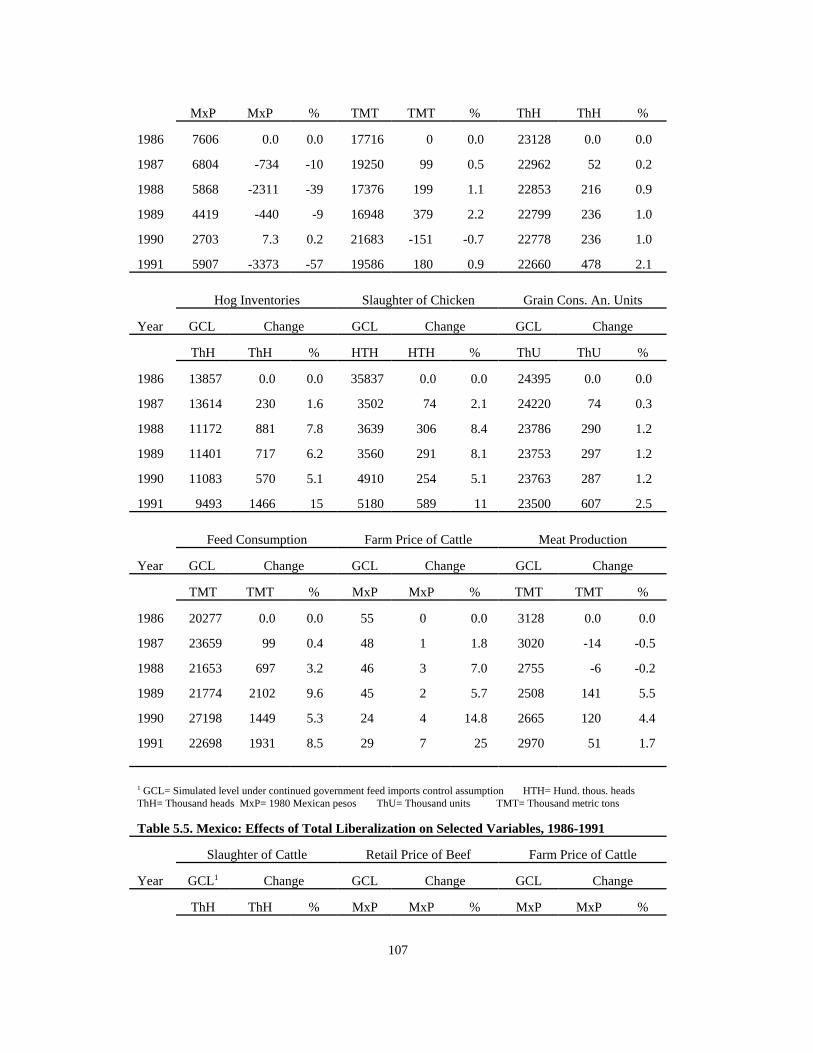
107
MxP MxP % TMT TMT % ThH ThH %
1986 7606 0.0 0.0 17716 0 0.0 23128 0.0 0.0
1987 6804 -734 -10 19250 99 0.5 22962 52 0.2
1988 5868 -2311 -39 17376 199 1.1 22853 216 0.9
1989 4419 -440 -9 16948 379 2.2 22799 236 1.0
1990 2703 7.3 0.2 21683 -151 -0.7 22778 236 1.0
1991 5907 -3373 -57 19586 180 0.9 22660 478 2.1
Hog Inventories Slaughter of Chicken Grain Cons. An. Units
Year GCL Change GCL Change GCL Change
ThH ThH % HTH HTH % ThU ThU %
1986 13857 0.0 0.0 35837 0.0 0.0 24395 0.0 0.0
1987 13614 230 1.6 3502 74 2.1 24220 74 0.3
1988 11172 881 7.8 3639 306 8.4 23786 290 1.2
1989 11401 717 6.2 3560 291 8.1 23753 297 1.2
1990 11083 570 5.1 4910 254 5.1 23763 287 1.2
1991 9493 1466 15 5180 589 11 23500 607 2.5
Feed Consumption Farm Price of Cattle Meat Production
Year GCL Change GCL Change GCL Change
TMT TMT % MxP MxP % TMT TMT %
1986 20277 0.0 0.0 55 0 0.0 3128 0.0 0.0
1987 23659 99 0.4 48 1 1.8 3020 -14 -0.5
1988 21653 697 3.2 46 3 7.0 2755 -6 -0.2
1989 21774 2102 9.6 45 2 5.7 2508 141 5.5
1990 27198 1449 5.3 24 4 14.8 2665 120 4.4
1991 22698 1931 8.5 29 7 25 2970 51 1.7
1 GCL= Simulated level under continued government feed imports control assumption HTH= Hund. thous. headsThH= Thousand heads MxP= 1980 Mexican pesos ThU= Thousand units TMT= Thousand metric tons
Table 5.5. Mexico: Effects of Total Liberalization on Selected Variables, 1986-1991
Slaughter of Cattle Retail Price of Beef Farm Price of Cattle
Year GCL1 Change GCL Change GCL Change
ThH ThH % MxP MxP % MxP MxP %

108
1986 6773 -451 -6.6 42 26 62 55 9 17
1987 6724 -656 -9.7 50 37 73 48 15 31
1988 6098 -461 -7.5 80 6 8 46 12 27
1989 6074 -344 -5.6 94 0.5 0.5 45 14 31
1990 5748 -500 -8.7 62 25 40 24 20 81
1991 6061 -493 -8.1 68 10 15 29 20 68
Cattle Inventories Grain Cons. An. Units Feed Consumption
Year GCL Change GCL Change GCL Change
ThH ThH % ThU ThU % TMT TMT %
1986 23128 53 0.2 24395 45 0.2 20277 0.0 0.0
1987 22962 170 0.7 24220 169 0.7 23659 183 0.7
1988 22853 349 1.5 23786 387 1.6 21653 862 3.9
1989 22799 397 1.7 23753 410 1.7 21774 2276 10
1990 22778 445 1.9 23763 431 1.8 27198 1683 6.1
1991 22660 699 3.1 23500 754 3.2 22698 2213 9.7
Producer Price of Feed Feed Production Meat Consumption
Year GCL Change GCL Change GCL Change
MxP MxP % TMT TMT % TMT TMT %
1986 7606 493 6.4 17716 0 0.0 3143 -101 -3.2
1987 6804 152 2.2 19250 183 0.9 3038 -174 -5.7
1988 5868 -1523 -25 17376 364 2.1 2784 -85 -3.1
1989 4419 498 11 16948 553 3.2 2538 40 1.6
1990 2703 1204 44 21683 82 0.3 2700 -55 -2.0
1991 5907 -2238 -37 19586 462 2.3 3009 -92 -3.1
1 GCL= Simulated level under continued government complete trade control assumptionThH= Thousand heads MxP= 1980 Mexican pesos ThU= Thousand units TMT= Thousand metric tons
Table 5.6. Mexico: Effects of a 3.6% Increase in Real Per Capita Income on SelectedVariables
Meat Consumption Retail Price of Beef Retail Price of Pork
Year TL1 Change TL Change TL Change
TMT TMT % MxP MxP % MxP MxP %

109
1986 2893 1 0.1 79 13.4 16 92 17.5 19
1987 2876 5 0.2 77 12.3 16 114 15.5 13
1988 2786 8 0.2 79 12.4 15 132 15.8 12
1989 2607 11 0.4 96 12.3 13 130 15.5 12
1990 2714 12 0.4 83 12.8 15 105 16.4 16
1991 2971 14 0.5 78 12.7 16 110 15.8 14
Retail Price of Chicken Cattle Inventories Slaughter of Cattle
Year TL Change TL Change TL Change
MxP MxP % ThH ThH % ThH ThH %
1986 50 1.7 3.3 23046 5 0.01 6030 -4.6 -0.07
1987 63 1.6 2.5 23089 7 0.03 5919 -0.4 -0.00
1988 69 1.7 2.4 23118 8 0.03 5660 1.5 0.02
1989 60 1.6 2.7 23162 9 0.04 5644 2.5 0.04
1990 49 1.8 3.6 23170 10 0.04 5254 3.0 0.05
1991 44 1.7 3.8 23271 10 0.04 5580 3.4 0.06
Grain Cons. An. Units Feed Consumption Feed Production
Year TL Change TL Change TL Change
ThU ThU % TMT TMT % TMT TMT %
1986 24342 8 0.03 20326 0 0.0 17765 0 0.0
1987 24409 13 0.05 23471 15 0.06 19062 15 0.07
1988 24120 15 0.06 22193 22 0.09 17418 22 0.12
1989 24174 16 0.06 24029 27 0.11 17480 27 0.15
1990 24172 18 0.07 28714 33 0.11 21598 33 0.15
1991 24178 18 0.07 24901 35 0.14 20038 35 0.17
1 TL= Historical level after 1986 trade liberalization ThH= Thousand heads MxP= 1980 Mexican pesos ThU= Thousand units TMT= Thousand metric tons
Table 5.7. Mexico: Impact of Changes in Real Per Capita Income on Meat Imports
Meat Imports Trade Lib. (High Income) Trade Lib. (Low Income)
Year GCL1 TL Change Change
Thous. Metric Tons TMT % TMT %
1986 16 16 65 411 -65 -411

110
1987 18 18 91 510 -91 -510
1988 29 81 107 132 -107 -132
1989 33 112 118 105 -118 -105
1990 40 99 127 128 -127 -127
1991 47 122 135 110 -135 -110
Table 5.8. Mexico: Impact of Changes in Real Per Capita Income on Cattle Exports
Cattle Exports Trade Lib. (High Income) Trade Lib. (Low Income)
Year GCL TL Change Change
Thousand Heads ThH % ThH %
1986 462 860 -47 -5.5 47 5.5
1987 457 1019 -42 -4.1 42 4.1
1988 451 981 -41 -4.2 41 4.2
1989 446 945 -39 -4.1 39 4.1
1990 440 1351 -40 -2.9 40 2.9
1991 435 1030 -37 -3.6 37 3.6
1 GCL= Assumed variable level under continued government control TL= Historical level after 1986 trade liberalization ThH= Thousand heads TMT= Thousand metric tons

111
Table 5.9. Mexico: Impact of Changes in Real Per Capita Income on Cattle Imports
Cattle Imports Trade Lib. (High Income) Trade Lib. (Low Income)
Year GCL1 TL Change Change
Thousand Heads ThH % ThH %
1986 57 57 47 83 -47 -83
1987 39 39 42 109 -42 -109
1988 42 218 41 19 -41 -19
1989 46 104 39 37 -39 -37
1990 50 354 40 11 -40 -11
1991 54 227 37 16 -37 -16
Table 5.10. Mexico: Impact of Changes in Real Per Capita Income on Feed Imports
Feed Imports Trade Lib. (High Income) Trade Lib. (Low Income)
Year GCL TL Change Change
Thous. Metric Tons TMT % TMT %
1986 3392 3392 88 2.6 -88 -2.6
1987 5317 5479 161 2.9 -161 -2.9
1988 5263 5879 226 3.8 -226 -3.8
1989 5895 7660 287 3.7 -287 -3.7
1990 6382 8017 361 4.5 -361 -4.5
1991 4067 6368 416 6.5 416 6.5
1 GCL= Assumed variable level under continued government control TL= Historical level after 1986 trade liberalization ThH= Thousand heads TMT= Thousand metric tons

112
SUMMARY AND CONCLUSIONS
A number of countries have formed or are negotiating the terms for trade associations of various types to stimulatetheir economies. Trade associations or agreements that reduce tariff and non-tariff barriers among countries allowfreer trade and increase the size of the market for goods and services of the participant countries. In North America,the U.S., Canada, and Mexico launched an experiment in regional free trade when the North American Free TradeAgreement (NAFTA) entered into force at the beginning of 1994.
This study provided a comprehensive, consistent assessment of the potential impacts of freer U.S.-Mexico agriculturaltrade on the Mexican livestock, meat, and feedgrain industries. Several research objectives were pursued in thisstudy, including the following: (1) a qualitative assessment of the economic structure and government policyintervention in the Mexican livestock, meat, and feedgrain industry; (2) the development of an econometric modelto measure and analyze the key parameters affecting the behavior of the demand, supply, prices, trade, and otherrelevant variables in the Mexican livestock, meat, and feedgrain markets; (3) validation of the econometric modelfor use in historical simulation analysis of Mexican markets for livestock, meat, and feedgrains; and (4) the analysisof the likely effects of freer U.S.-Mexico trade through model simulation analyses under several different scenarios.
The first objective was achieved in the background section by presenting the characteristics of the Mexican livestock,meat, and feedgrain sectors and by providing the basis for the hypothetical model subsequently defined. Among themain conclusions of the qualitative assessment of the Mexican livestock, meat, and feedgrain industries found in thebackground section are the following:
1. The growth and development of the Mexican meat and livestock industries prompted the development andexpansion of the Mexican feedgrain industry during the 1970s. This expansion was slowed by the 1982economic crisis in Mexico.
2. Although beef had been the meat traditionally consumed by Mexicans, pork became the most consumed meatduring the 1970s and 1980s fostered by the rapid development of the Mexican hog industry during the 1970sand 1980s. Following the 1982 economic crisis, however, chicken emerged as a cheap and increasingly popularmeat alternative in Mexico.
3. Mexican government domestic and trade policies prior to the unilateral opening of Mexican markets restrictedthe trade meat and livestock as well as of feedgrains in order to maintain low meat prices or to enforce the"guaranteed price" policy for feedgrains.
4. The main components of balanced animal feed rations in Mexico are sorghum and soymeal. Corn is the majorstaple food in Mexico so that corn is not commonly used in feed formulations.
5. PROCAMPO is the latest program of the Mexican government intervention in agriculture. This program intendsto gradually eliminate the guaranteed price scheme and to bring Mexican agricultural prices to a world level.
The model section achieved the second objective and presented a conceptual model of the Mexican livestock, meat,and feedgrain sectors. The underlying assumptions of the model were presented first and then the livestock and meatsupply relationships were discussed. The supply and demand model for the feedgrain sector was also presented. Theresults of three meat demand model formulations (LA/AIDS, ROTTERDAM, and single equation) for the Mexicanmeat sector were then presented and compared. Finally, an integrated supply and demand model for each of the meatdemand specifications was presented.
The empirical analysis section focused on the third objective of the study and presented the results of the empiricalestimation of the alternative conceptual models of the Mexican livestock, meat, and feedgrain industries presented

113
in the previous chapter. Data issues were addressed first focusing on the lack of reliability of official Mexican data.Issues and procedures for econometric estimation of the coefficients of the alternative models were then considered,especially the issues of structural change and endogeneity of the prices in the demand models. Econometricconsiderations, including the differences among several estimation techniques such as OLS, ILS, 2SLS, SUR, and3SLS, were discussed. The three alternative models for Mexican meat demand as formulated conceptually in theprevious chapter were used to test for structural change. The results failed to provide strong evidence of structuralchange in Mexican meat demand behavior due to the 1982 economic crisis or to the trade liberalization that beganin 1986.
Parameters for the three model specifications were estimated using both SUR and 3SLS. Problems of grosscomplementarity among the different types of meat plagued both the AIDS and the ROTTERDAM results. TheMexican meat demand model was also tested for price endogeneity using the Hausman specification test.The resultsof the Hausman test indicate that the parameters obtained by using SUR estimation are consistent and prices in theMexican meat demand model may treated as exogenous when the demand model is estimated independently.However, when estimation of livestock and meat supply and demand is required, 3SLS estimation technique isencouraged.
The three alternative model specifications for meat demand were then integrated into the livestock and meat supplyand feedgrain components of the model. The plan was to simulate all three models over the historical period andconduct sensitivity analyses as a means of selecting among the models for use in the subsequent simulation analysis.Unfortunately, both the model with the AIDS meat demand system formulation and the model with theROTTERDAM meat demand formulation failed to converge in simulation. The cause of the failure to converge wasprimarily the high degree of complementarities among meats in the demand systems which forced a number of theendogenous variables like meat prices away from rather than towards an equilibrium solution. Only the model withthe single equation LINEAR meat demand system specification converged and simulated over the entire period ofthe data and, thus, by default was selected for use in the subsequent simulation analysis.
Among the principal results drawn from the empirical estimation of the coefficients of the model with the singleequation meat demand system were the following:
1. Mexican cattle inventories have been highly unresponsive to changes in Mexican cattle and feed prices reflectingthe effects of Mexican meat price and trade controls.
2. The slaughter of cattle in Mexico is primarily determined by cattle supply although Mexican cattle and beefprices have had some affect on cattle slaughter in Mexico over time.
3. The response of Mexican hog inventories to Mexican hog and feed prices have been somewhat higher than thecorresponding response of cattle inventories. Mexican price and trade controls on hog and pork have been lessextensive than for cattle and beef. Also, the estimation results indicate that hog slaughter in Mexico has beendetermined primarily by the supply available for slaughter.
4. The per capita consumption of beef and pork in Mexico are positively affected by changes in per capita income.The gross income elasticity for beef is 0.7 while that of pork is 2.91. The higher income response of pork isexplained by the fact that higher pork prices, especially of those of bacon, ham, and other derivatives may bepurchased only by those high-income consumers.
5. Changes in feed prices have had little effect on the area harvested of the feedgrains in Mexico. Again, Mexicanpolicies, including guaranteed prices and import restrictions, have reduced the historical importance of pricechanges in acreage decision of farmers.
Simulation statistics, including the RMS% error and the Theil coefficients, indicated a good performance of the modelin tracking the historical data for prices. Sensitivity analysis indicated that the model is highly stable.

114
The fourth and final objective of the study was achieved in the simulation analysis section in which the results ofusing the Mexican livestock, meat, and feedgrain model to simulate the effects of trade liberalization in Mexico werepresented. Because a complete, consistent series of data for those sectors is not yet available for the period sinceNAFTA took effect in January of 1994, the analysis considered only the pre-NAFTA period of Mexican unilateralliberalization. The results, however, provided important insights into the effects of liberalization under NAFTA forthe Mexican livestock, meat, and feedgrain sectors. In order to isolate the specific effects of liberalization of tradein each of those sectors as well as the aggregate overall effects of liberalization on all sectors, the results of 5 differentsimulation scenarios were presented: (1) liberalization of only cattle exports from Mexico; (2) liberalization of onlycattle imports by Mexico; (3) liberalization of only meat imports by Mexico; (4) liberalization of only feed importsby Mexico; and, (5) liberalization of exports and imports of cattle, meat, and feed simultaneously.
In general, the analysis indicated that the Mexican policy shift to more open markets substantially impacted Mexicanlivestock, meat, and feedgrain trade. The results also clearly indicated that the effects of liberalizing Mexicanlivestock, meat, and feedgrain trade were highly dependent on the level and direction of change in per capita incomeduring the period of liberalization. More specifically, the simulation results indicated the following:
1. The Mexican comparative advantage is in the production of feeder cattle for export rather than for domesticfeeding and slaughter.
2. Liberalization of Mexican markets benefits both the livestock and feedgrain sectors in Mexico.
3. Liberalization of Mexican markets also benefits the Mexican meat processing industry.
4. Liberalization of Mexican livestock, meat, and feedgrain markets generates little effect on the Mexican feedgrainsector because the positive price effects of an increase in feed demand from increased cattle inventories arelargely offset by the negative price effects of an increase in feed imports.
5. Changes in real per capita income in Mexico are an important factor in determining the likely consequences oftrade liberalization on Mexican meat import imports. For example, if Mexican per capita income had been only1 standard deviation lower than was actually the case during the 1986 to 1991 period of unilateral tradeliberalization, the model simulation results indicate that Mexican meat demand would have dropped enough toeliminate meat imports altogether possibly even creating excess Mexican supplies of meat for export.
6. Imports of both Mexican cattle and feedgrains are positively associated with changes in income in Mexico.
7. Even though feed prices are positively affected by trade liberalization in the meat, livestock, and feedgrainmarkets, Mexican feed production responds more to variables such as the cost and availability of credit, the costof other inputs, and government farm policies than to prices.
Limitations of the Study
Modelling the livestock and agricultural sectors in Mexico is a difficult process. Lack of literature, lack of reliabledata, and the inability and unwillingness of Mexican government officials to cooperate makes such a study a nearlyimpossible task. Several limitations or shortcomings of this study should be noted.
First, Mexico suffered several economic crises between 1971 and 1991 which were accompanied by hugedevaluations of the Mexican peso and high rates of inflation. These two factors caused serious, although usuallytemporary, trade distortions. Trade policy changes in 1986 also brought changes in agricultural trade levels. The testconducted for structural change was intended to determine if those events affected Mexican meat consumptionbehavior. Although no evidence of structural change was found in the analysis, the test was limited to measuringparameter stability by using intercept and/or slope shifters due to the small number of observations (20). A largernumber of observations would have allowed the use of more sophisticated techniques to test for structural change.

115
Second, several modifications were made to the conceptual model presented in the model section for the empiricalestimation reported in the empirical analysis section as a result of the unavailability of needed data series. Forexample, breeding, feeder, and fed cattle inventories could not be separately identified. Consequently, only one"cattle inventory" behavioral equation was estimated. Also, data for area planted and feed and non-feed demand ofthe different crops were not available or incomplete. Although corn has been in animal feed rations in Mexico, nodata is available on the feeding of corn. Data for the number of grass-fed versus grain-fed cattle in Mexico are alsolargely unavailable or unreliable.
Third, price data were obtained from several sources causing a degree of inconsistency. Meat and livestock priceswere supplied by the Colegio de Posgraduados in Chapingo while most feed prices were estimated by dividing dataon crop value and crop production appeared in the Mexican Presidential Report. Also, due to the high rates ofinflation that existed in Mexico during the sample period (1971 to 1991), prices had to be deflated. Meat prices weredeflated using a general consumer price index while livestock and feed prices were deflated using a general wholesaleprice index.
Fourth, the empirical model used for the simulation analyses was selected by default since two of the three alternativemodels failed to converge in simulation. Consequently, a comparison of the simulation performance of models ofthe Mexican livestock, meat, and feedgrain industries that included complete meat demand systems against the modelincluding a single equation meat demand formulation was not possible.
Fifth, the low estimated price response of livestock inventories, livestock slaughter, and feedgrain area harvestedreflects the effects of government policies that existed during the period of the data. Given the recent changes ingovernment policy, including elimination of CONASUPO and production input subsidies, the implementation ofPROCAMPO, the privatization of agricultural institutions, and the further liberalization of trade under NAFTA,among other things, the responsiveness of market agents to price signals has likely changed since the late 1980s andearly 1990s. Unfortunately, data is available only with long lags in Mexico. When a reliable set of complete databecomes available for a more recent period, tests for such changes in behavioral parameters will need to be done.
Sixth, development of the livestock and the feed production models included the assumption of adaptive expectationsin livestock production and naive expectations in feedgrain production consistent with similar studies for othercountries. The performance of these expectations models against other possible models was not tested.
Seventh, for simplicity, the model developed assumed that several variables such as macroeconomic variables andtechnologically derived yields were exogenous. A more extensive model with an endogenous macroeconomiccomponent would have provided the ability to conduct more extensive tests of the relationship between the Mexicanmacroeconomy and Mexican livestock, meat, and feedgrain trade.
Eighth, weights developed by the U.S. Department of Agriculture to calculate the number of U.S. grain-consuminganimal units from data on U.S. livestock inventories were used to calculate Mexican grain-consuming animal units.The relevance of those weights for Mexico is not clear. Also, the weights used to calculate the producer price of feedwere considered to be fixed over the entire sample.
Ninth, the effects of trade liberalization were analyzed against assumptions regarding what the level of livestock,meat, and feedgrain trade would have been in the absence of the policy of unilateral trade liberalization during 1986through 1991. Although the assumptions were based on past performance of trade before liberalization, in the end,the simulated results are as arbitrary as the assumptions made. However, only the magnitudes and not the directionsof change are dependent on those assumptions.
Finally, a dearth of previous quantitative studies on the Mexican livestock, meat, and feedgrain industries preventeda comparison of the results found in this study. Consequently, this study might be considered a benchmark for futureanalyses of those industries and of the effects of freer trade.
Suggestions for Further Research

116
The qualitative and empirical analyses presented in this study provide a more complete understanding of the behaviorof the Mexican livestock, meat, and feedgrain markets. The research also presented an in depth analysis of thepossible consequences of trade liberalization and changes in per capita income on those markets. The limitations ofthe study provide a starting point for future research efforts. Some other areas, including the following, might alsoprove fruitful for future research.
First, a more complete and consistent data series is needed for the Mexican agricultural sector in general. Acombination of efforts by Mexican federal and state government agencies, crop producer associations, and livestockand meat federations is needed. Otherwise, poor data on Mexican agricultural markets will continue to hamperresearch efforts and limit confidence in analytical results using the available data.
Second, although agricultural trade is expected to intensify under NAFTA, the effects will be highly dependent onthe performance of the Mexican economy as suggested in this study. Given the severe economic conditions of 1995in Mexico, an updated study using more recent data will be needed to separate the trade effects of NAFTA and thoseof the Mexican economy.
Third, additional scenarios could be simulated to analyze the effects of specific tariff or trade barrier reductions,changes in the value of the peso, and other relevant issues affecting Mexican livestock, meat, and feedgrain trade.
Fourth, a more in depth analysis of the Mexican meat demand system in Mexico is needed. The use of other tests forstructural change, variations in the complete demand system specifications, and disaggregation of meat consumptionby geographical region, economic level, and demographic factors could provide a better explanation of the meatconsumption behavior in Mexico.
Finally, a natural extension of this research would be the application of similar techniques used in this study to otheragricultural products such as fruits and vegetables which are important part of U.S.-Mexico agricultural trade.

117
REFERENCES
Arzac, E.R. and M. Wilkinson, "A Quarterly Econometric Model of the United States Livestock and Feed GrainMarkets and Some of Its Policy Implications," Amer. J. Agr. Econ. 61(1979):297-308.
Azzam, A., J.F. Yanagida, and D. Linsenmeyer, "A Linked Econometric Model of the Livestock-Feed Sector inNebraska and the Rest of the United States," North Central J. Agr. Econ. 9(1987):247-258.
Boadu, F.O., The U.S.-Mexico Free Trade Agreement: Legal Issues for Agriculture, TAMRC Report No. IM-9-91,Texas Agricultural Market Research Center, Texas A&M University, April 1991.
Brandt, J.A., R.E. Young II, S. Alam, A.W. Womack, "Foreign Trade and Its Impact on the Domestic LivestockMarket," The Economics of Meat Demand, Reuben C. Buse, ed., Proceedings of the Conference on TheEconomics of Meat Demand. October 20-21, 1986. Charleston, South Carolina.
Braschler, C. "The Changing Demand Structure for Pork and Beef in the 1970s: Implications for the 1980s." South.J. of Agr. Econ. 15(1983):105-110.
Bredahl, M.E., A. Burst, and P.F. Warnken, Growth and Structure of the Mexican Cattle Industry. Special Report317, University of Missouri-Columbia. January, 1985.
Burst, A.C., M.E. Bredahl, and P.F. Warnken, Growth and Structure of the Mexican Feedstuffs industry. SpecialReport 315, University of Missouri-Columbia. November, 1984.
Canacintra, La Industria Alimenticia Animal en Mexico. Seccion de Fabricantes de Alimentos Balanceados paraAnimales, 1981-82 and 1991-92.
Capps, Jr., O., R. Tsai, R. Kirby, and G. Williams, "A Comparison of Demands for Meat Products in the Pacific RimRegion." J. of Agr. and Resource Econ. 1(1994):210-224.
Chauvet-Sanchez, Michelle. "¿La Ganadería Nacional en Vías de Extinción?." Comercio Exterior vol. 40, num. 9,Mexico, septiembre de 1990:868-875.
Chavas, J.P., "Structural Change in the Demand for Meat." Amer. J. Agr. Econ. 65(1983):148-153.
Chavas, J.P., "On the Structure of Demand for Meat" The Economics of Meat Demand, Reuben C. Buse, ed.,Proceedings of the Conference on The Economics of Meat Demand. October 20-21, 1986:125-135. Charleston,South Carolina.
Deaton, A.S. and Muellbauer. Economics and Consumer Behavior. Cambridge: Cambridge University Press, 1980.
Eales, J.S. and L.J. Unnevehr, "Demand for Beef and Chicken Products: Separability and Structural Change." Amer.J. Agr. Econ. August 70(1988):521-532.
Egbert, A.C. and S. Reutlinger, "A Dynamic Long-Run Model of the Livestock-Feed Sector," J. of Food Econ.47(1965):1288-1305.
Engels, C. and E. Segarra, "Government Intervention in the Mexican Livestock Sector," Final Report, Texas Tech,Lubbock, Texas. September 1989.
Freebairn, J.W. and G. Rausser, "Effects of Changes in the Level of U.S. Beef Imports," Amer. J. Agr. Econ.57(1975):676-688.

118
Fuller, S.W. and C.R. Hall, The U.S.-Mexico Free Trade Agreement: Issues and Implications for the U.S. and TexasFresh Vegetable/Melon Industry, TAMRC Report No. IM-2-91, Texas Agricultural Market Research Center,Texas A&M University, April 1991.
Fuller, S.W., The U.S.-Mexico Free Trade Agreement: Agricultural Transportation Issues, TAMRC Report No. IM-7-91, Texas Agricultural Market Research Center, Texas A&M University, April 1991.
Garcia Mata, R. and E. Lopez Lopez, Algunos Aspectos de la Ganaderia en Mexico. Colegio de Postgraduados.Centro de Economia. Chapingo, Mexico. 1991.
Garcia Vega, J.J., "Elasticidades, Flexibilidades y Cambio Estructural en la Industria de la Carne de los EstadosUnidos de America." IV Encuentro Internacional de Investigadores en Economia Agricola. UniversidadAutonoma de Tamaulipas, Mexico. 1993:125-137.
Gomez Cruz, M.A., J.J. Flores Verduzco, and R.S. Rindermann, "Tendencias y Opciones de la Produccion de Carnede Puerco, Pollo y Huevo en Mexico." Comercio Exterior, vol. 40, num. 9, Mexico, Sep. 1990: 876-885.
Gong, S.C., "The Taiwanese Livestock and Feedgrain Markets and Policies." Ph.D. thesis, Iowa State University,Ames, Iowa, 1988.
Goodwin, H.L., Jr., The U.S.-Mexico Free Trade Agreement: Agricultural Labor Issues, TAMRC Report No. IM-11-91, Texas Agricultural Market Research Center, Texas A&M University, April 1991.
Hahn, W.F., "Effects of Income Distribution on Meat Demand." J. of Agr. Econ. Research. 40(1988):19-24. Hausman, J.A., "Specification Tests in Econometrics." Econometrica 46(1978):1251-71.
Heien, D., "Seasonality in U.S. Consumer Demand." J. of Bus. and Econ. 1(1983):280-284.
Heien, D., L.S. Jarvis, and F. Perali, "Food Consumption in Mexico." Food Policy. 14(1989):167-179.
Instituto Nacional de Estadistica, Geografia e Informatica (INEGI), Encuesta Nacional de Ingresos y Gastos de losHogares, fourth quarter, Mexico City, Mexico, 1984.
Jarvis, L.S., "Cattle as Capital Goods and Ranchers as Portfolio Managers: An Application to the Argentine CattleSector." J. of Pol. Econ. 82(1974):489-520.
Johnson, S.R., A. Hassan, and R.D. Green, Demand Systems Estimation. Methods and Applications. Iowa StateUniversity, Ames, Iowa.1984.
Krissoff, B, P. Liapas, J. Link, and L. Neff, "Implications of a U.S.-Mexican Free Trade Pact: Some PreliminaryEvidence for Agriculture," Selected Paper Presented at the 1991 Southern Agricultural Economic AssociationMeetings, Fort Worth, Texas.
Kulshreshtha, S.N. and A.G. Wilson, "An Open Econometric Model of the Canadian Beef Cattle Sector," Amer. J.Agr. Econ. 54(1972):84-91.
Leuck, D.J., "Analysis of the Feed-Livestock Sector of the European Community," ERS Staff Report No.AGES840529, ERS, USDA, Jan. 1985.
Lich, G.E. and J.A. McKinney, eds., "Free Trade and the United States - Mexico Borderlands," Baylor University,Regional Report prepared for the Subcommittee on Economic Growth, Trade, and Taxes of the Joint EconomicCommittee, U.S. Congress, July 1, 1991.

119
Lyford, C.P., "Forecasting Mexican Imports of U.S. Corn, Sorghum, and Soybeans Under Free Trade and DebtReduction Scenarios," M.S. Thesis, Texas A&M University, College Station, Texas, 1991.
Martin, W.J. and E.O. Heady, "A Quarterly Model of the U.S. Livestock-Feed Subsector and Some of Its DynamicMultipliers," CARD Report No. 127T, Iowa State University, Ames, Iowa.1984.
Minert, J., C. Snyder, B. Goodwin, and Gary Brester, "Meat Demand in Mexico." Selected Paper Presented at the1994 Southern Agricultural Economics Association Meetings, Nashville, Tennessee.
Moschini, G. and K.D. Meilke, "Parameter Stability and the U.S. Demand for Beef." West. J. of Agr. Econ.9(1984):271-282.
Nacional Financiera. "Foro de Consulta sobre las Relaciones de México con el Mundo" El Mercado de Valores. Num9. Año L. May 1990:3-10.
Nyankori, J.C.O. and G.H. Miller, "Some Evidence and Implications of Structural Change in Retail Demand forMeats." South J. of Agr. Econ. 14(1982):65-70.
Ozuna, T. and R. Guajardo Q., The U.S.-Mexico Free Trade Agreement: Natural Resource and Environmental Issues,TAMRC Report No. IM-8-91, Texas Agricultural Market Research Center, Texas A&M University, April 1991.
Perez-Espejo, R., "El Sector Pecuario en México: Características y Perspectivas," Comercio Exterior Vol. 38, No.8, August 1988:686-693.
Pindyck, R.S. and D.L. Rubinfeld. Econometric Models and Economic Forecasts. Third Edition, New York: McGrawHill, Inc. 1991.
Polyconomics, Mexico 2000: A Classical Analysis of the Mexican Economy and the Case for Supply-Side EconomicReforms, Morristown, New Jersey, July 1990.
Robinson, S., M.E. Burfisher, Hinojosa-Ojeda, R., and K.E. Thierfelder, "Agricultural Policies and Migration in aU.S.-Mexico Free Trade Area: A Computable General Equilibrium Analysis," Working Paper No. 617,Department of Agricultural and Resource Economics, University of California at Berkeley, December 1991.
Rosson, C.P. III and A.L. Angel, The U.S.-Mexico Free Trade Agreement: General Economic Issues, TAMRCReport No. IM-12-91, Texas Agricultural Market Research Center, Texas A&M University, April 1991.
Rosson, C.P. III, B.K. Schulthies, and D. White, The U.S.-Mexico Free Trade Agreement: Issues and Implicationsfor the U.S. and Texas Livestock and Meat Industry, TAMRC Report No. IM-5-91, Texas Agricultural MarketResearch Center, Texas A&M University, April 1991.
Salinas de G., Carlos, Informe de Gobierno, Mexico. Presidencia de la Republica. 1993-94. Private Colection, J.Garcia Vega.
Schulthies, B.K. and R.B. Schwart, The U.S.-Mexico Free Trade Agreement: Issues and Implications for the U.S.and Texas Dairy Industry, TAMRC Report No. IM-10-91, Texas Agricultural Market Research Center, TexasA&M University, August 1991.
Sek, L., "Mexico-U.S. Free Trade Agreement?" Congressional Research Service, Library of Congress, Report 90-450E, IB90140, November 7, 1990.

120
Stern, R.M., "A North American Free Trade Agreement: Issues and Assessment," Paper presented at a meeting ofthe North American Institute, Winners and Losers: Readjustment Mechanisms in a North American Free TradeAgreement, Monterrey, Mexico, May 17-19, 1991.
Taylor, M.J., The U.S.-Mexico Free Trade Agreement: Issues and Implications for the U.S. and Texas CottonIndustry, TAMRC Report No. IM-6-91, Texas Agricultural Market Research Center, Texas A&M University,April 1991.
Thompson, G.D. and P.L. Martin, "The Potential Effects of Labor-Intensive Agriculture in Mexico on United States-Mexico Migration," Commission for the Study of International Migration and Cooperative EconomicDevelopment, Washington, D.C., Working Paper No. 11, December 1991.
Thompson, R.L., "A Survey of Recent U.S. Developments in International Agriculture Trade Models,"Bibliographies and Literature of Agriculture No. 21, ERS, USDA, September 1981.
Tsai, Reyfong, "Taiwanese Livestock and Feedgrain Markets: Economic Structure, Policy Intervention, and TradeLiberalization," PhD dissertation, Texas A&M University, College Station, Texas, 1994.
U.S. Department of Agriculture (USDA), Economic Research Service, PS&D View. Mexico: Livestock Data, 1994.
U.S. Department of Agriculture, "Livestock-Feed Relationships." Economic Research Service. Statistical Bulletin#530.1974.
U.S. Department of Agriculture, Agricultural Statistics. 1971-1992.
U.S. Department of Agriculture, "Agriculture in a North American Free Trade Agreement," An Interim Review,Washington, D.C., April 1991.
U.S. International Trade Commission (USITC). Review of Trade and Investment Liberalization Measures by Mexicoand Prospects for Future United States- Mexico Relations, Phase I: Summary of Views on Prospects for FutureU.S. Mexico Relations. USITC Publication 2326, April 1990a.
U.S. International Trade Commission (USITC). Review of Trade and Investment Liberalization Measures by Mexicoand Prospects for Future United States- Mexico Relations, Phase I: Recent Trade and Investment ReformsUndertaken by Mexico and Implications for the United States. USITC Publication 2275, April 1990b.
U.S. International Trade Commission (USITC). Review of Trade and Investment Liberalization Measures by Mexicoand Prospects for Future United States- Mexico Relations, Phase II: Summary of Views on Prospects for FutureU.S. Mexico Relations. USITC Publication 2326, October 1990.
U.S. International Trade Commission (USITC). The Likely Impact on the United States of a Free Trade Agreementwith Mexico. Investigation No. 332-297, USITC Publication 2353, February 1991.
U.S. General Accounting Office (USGAO). U.S.-Mexico Trade: Trends and Impediments in Agricultural Trade.GAO/NSIAD-90-85BR, January 1990.
Universidad Autonoma de Chapingo, Bonanza y Crisis de la Ganadería Nacional, Montecillo, Mexico. 1989.
Wahl, T.I., "Modeling Dynamic Adjustment in Japanese Livestock Markets under Trade Liberalization," PhDdissertation, Iowa State University, Ames, Iowa.1989.

121
Waller, M.L., G.W. Williams, and D. White, The U.S.-Mexico Free Trade Agreement: Issues and Implications forthe U.S. and Texas Grains and Feeds Industry, TAMRC Report No. IM-4-91, Texas Agricultural MarketResearch Center, Texas A&M University, April 1991.
Weintraub, S. ed., U.S.-Mexican Industrial Integration: The Road to Free Trade. Boulder, Colo.: Westview Press,1991.
Williams, G.W. and C.P. Rosson III, The U.S.-Mexico Free Trade Agreement: Issues and Implications for U.S. andTexas Agriculture, TAMRC Report No. IM-1-91, Texas Agricultural Market Research Center, Texas A&MUniversity, April 1991.
Wohlgenant, M.K. and W.F. Hahn, "Dynamic Adjustments in Monthly Consumer Demands for Meats." Amer. J. Agr.Econ. 64(1982):553-557.