the method of least squares - forside · minimize the sum of the square of the distances between...
TRANSCRIPT

The Method of Least Squares
Lectures INF2320 – p. 1/80

The method of least squares
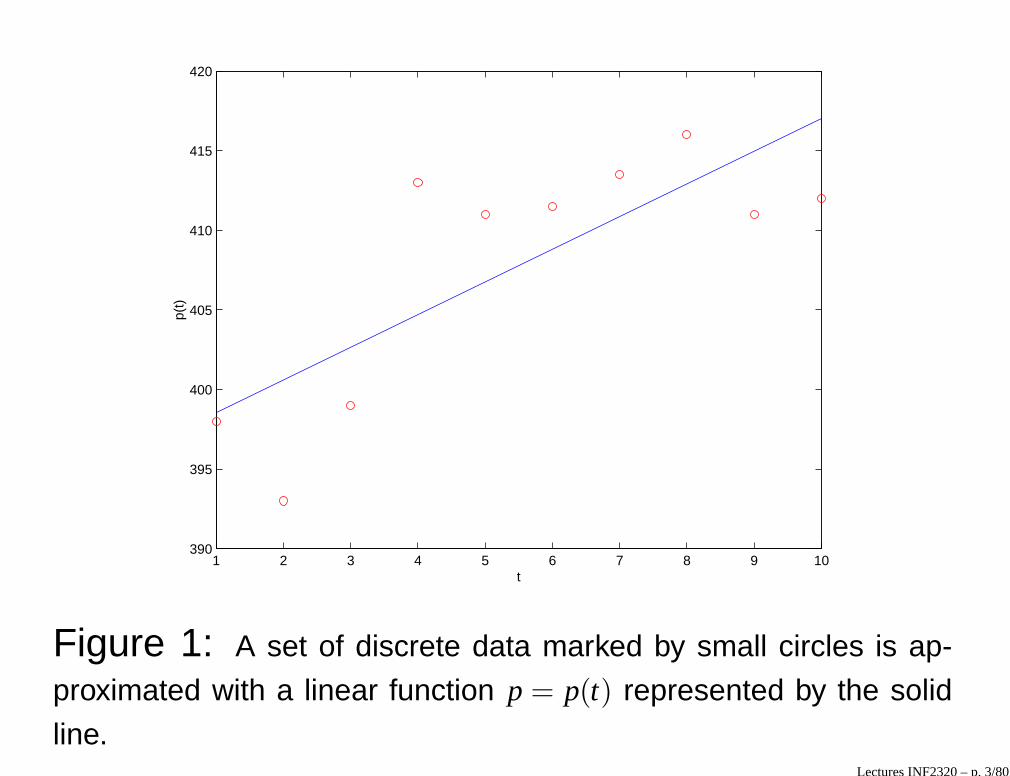
We study the following problem:Given n points (ti,yi) for i = 1, . . . ,n in the (t,y)-plane. Howcan we determine a function p(t) such that
p(ti) ≈ yi, for i = 1, . . . ,n? (1)
Lectures INF2320 – p. 2/80
1 2 3 4 5 6 7 8 9 10390
395
400
405
410
415
420
t
p(t)
Figure 1: A set of discrete data marked by small circles is ap-
proximated with a linear function p = p(t) represented by the solid
line.Lectures INF2320 – p. 3/80
1 2 3 4 5 6 7 8 9 10390
395
400
405
410
415
420
t
p(t)
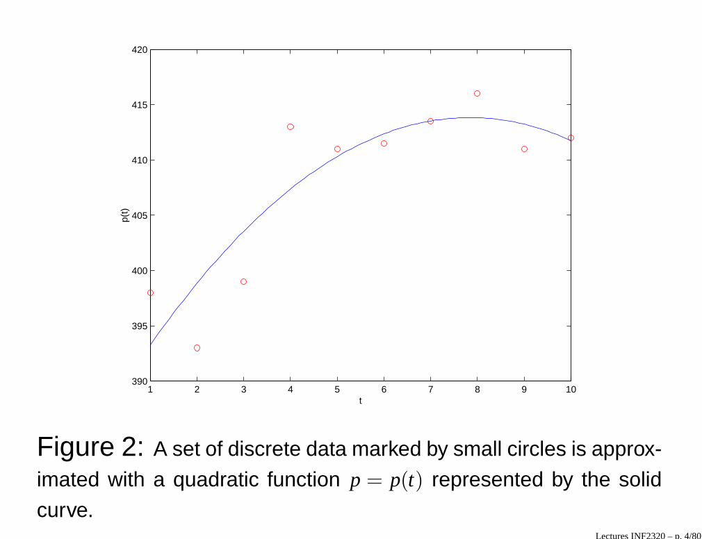
Figure 2: A set of discrete data marked by small circles is approx-
imated with a quadratic function p = p(t) represented by the solid
curve.Lectures INF2320 – p. 4/80

The method of least square
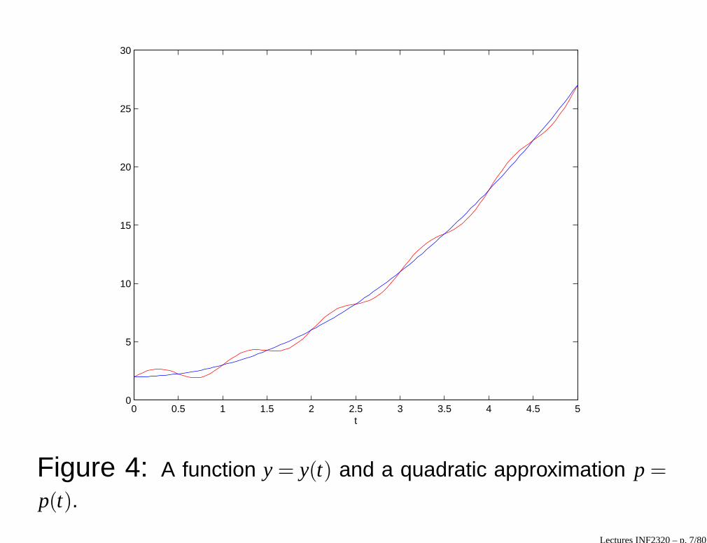
• Above we saw a discrete data set being approximatedby a continuous function
• We can also approximate continuous functions bysimpler functions, see Figure 3 and Figure 4
Lectures INF2320 – p. 5/80

0 0.5 1 1.5 2 2.5 3 3.5 4 4.5 50
1
2
3
4
5
6
7
8
t
Figure 3: A function y = y(t) and a linear approximation p = p(t).
Lectures INF2320 – p. 6/80
0 0.5 1 1.5 2 2.5 3 3.5 4 4.5 50
5
10
15
20
25
30
t
Figure 4: A function y = y(t) and a quadratic approximation p =
p(t).
Lectures INF2320 – p. 7/80

World mean temperature deviations
Calendar year Computational year Temperature deviation
ti yi
1991 1 0.29
1992 2 0.14
1993 3 0.19
1994 4 0.26
1995 5 0.28
1996 6 0.22
1997 7 0.43
1998 8 0.59
1999 9 0.33
2000 10 0.29
Table 1: The global annual mean temperature deviation measured
in ◦C for years 1991-2000.
Lectures INF2320 – p. 8/80

1991 1992 1993 1994 1995 1996 1997 1998 1999 20000
0.1
0.2
0.3
0.4
0.5
0.6
0.7
Figure 5: The global annual mean temperature deviation mea-
surements for the period 1991-2000.Lectures INF2320 – p. 9/80
Approximating by a constant
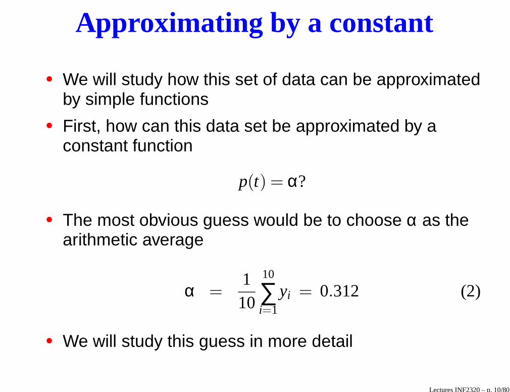
• We will study how this set of data can be approximatedby simple functions
• First, how can this data set be approximated by aconstant function
p(t) = α?
• The most obvious guess would be to choose α as thearithmetic average
α =110
10
∑i=1
yi = 0.312 (2)
• We will study this guess in more detail
Lectures INF2320 – p. 10/80

Approximating by a constant
• Assume that we want the solution to minimize thefunction
F(α) =10
∑i=1
(α− yi)2 (3)
• The function F measures a sort of deviation from α tothe set of data (ti,yi)
10i=1
• We want to find the α that minimizes F(α), i.e. we wantto find α such that F ′(α) = 0
• We have
F ′(α) = 210
∑i=1
(α− yi) (4)
Lectures INF2320 – p. 11/80
Approximating by a constant
• This leads to
210
∑i=1
α∗ = 210
∑i=1
yi, (5)
or
α∗ =110
10
∑i=1
yi, (6)
which is the arithmetic average
Lectures INF2320 – p. 12/80

0.1 0.2 0.3 0.4 0.5 0.60
0.1
0.2
0.3
0.4
0.5
0.6
0.7
0.8
0.9
1
α*=0.312
Figure 6: A graph of F = F(α) given by (3).
Lectures INF2320 – p. 13/80

Approximating by a constant
• Since
F ′′(α) = 210
∑i=1
1 = 20 > 0, (7)
it follows that the arithmetic average is the minimizerfor F
• We can say that the average value is the optimalconstant approximating the global temperature
• This way of defining an optimal constant, where weminimize the sum of the square of the distancesbetween the approximation and the data, is referred toas the method of least squares
• There are other ways to define an optimal constant
Lectures INF2320 – p. 14/80
Approximating by a constant
• Define
G(α) =10
∑i=1
(α− yi)4 (8)
• G(α) also measures a sort of deviation from α to thedata
• We have that
G′(α) = 410
∑i=1
(α− yi)3 (9)
• And in order to minimize G we need to solve G′(α) = 0,(and check that G′′(α) > 0)
Lectures INF2320 – p. 15/80
Approximating by a constant
• Solving G′(α) = 0 leads to a nonlinear equation thatcan be solved with the Newton iteration from theprevious lecture
• We use Newton’s method with• initial approximation: α0 = 0.312• tolerance specified by: ε = 10−8
This gives α∗ ≈ 0.345, in three iterations• α∗ is a minimum of G since
G′′(α∗) = 1210
∑i=1
(α∗− yi)
2 > 0
Lectures INF2320 – p. 16/80

0.1 0.2 0.3 0.4 0.5 0.60
0.05
0.1
0.15
α*=0.345
Figure 7: A graph of G = G(α) given by (8).
Lectures INF2320 – p. 17/80

1991 1992 1993 1994 1995 1996 1997 1998 1999 20000
0.1
0.2
0.3
0.4
0.5
0.6
0.7
Figure 8: Two constant approximations of the global annual mean
temperature deviation measurements from year 1991 to 2000.
Lectures INF2320 – p. 18/80

Approximating by a linear function
• Now we will study how we can approximate the worldmean temperature deviation with a linear function
• We want to determine two constants α and β such that
p(t) = α+βt (10)
fits the data as good as possible in the sense of leastsquares
Lectures INF2320 – p. 19/80
Approximating by a linear function
• Define
F(α,β) =10
∑i=1
(α+βti − yi)2 (11)
• In order to minimize F with respect to α and β, we cansolve
∂F∂α
=∂F∂β
= 0 (12)
Lectures INF2320 – p. 20/80

Approximating by a linear function
We have that
∂F∂α
= 210
∑i=1
(α+βti − yi), (13)
and therefore the condition ∂F∂α = 0 leads to
10α+
(
10
∑i=1
ti
)
β =10
∑i=1
yi. (14)
Lectures INF2320 – p. 21/80
Approximating by a linear function
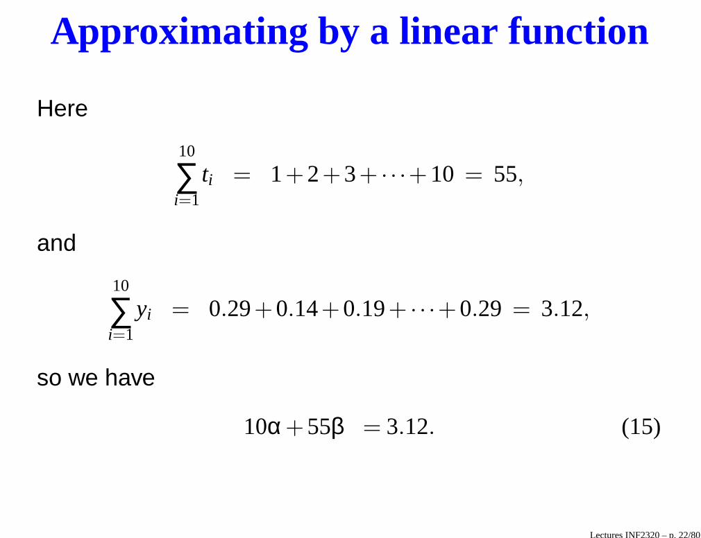
Here
10
∑i=1
ti = 1+2+3+ · · ·+10 = 55,
and
10
∑i=1
yi = 0.29+0.14+0.19+ · · ·+0.29 = 3.12,
so we have
10α+55β = 3.12. (15)
Lectures INF2320 – p. 22/80

Approximating by a linear function
Further, we have that
∂F∂β
= 210
∑i=1
(α+βti − yi)ti,
and therefore the condition ∂F∂β = 0 gives
(
10
∑i=1
ti
)
α+
(
10
∑i=1
t2i
)
β =10
∑i=1
yiti.
Lectures INF2320 – p. 23/80

Approximating by a linear function
We can calculate
10
∑i=1
t2i = 1+22 +32 + · · ·+102 = 385,
and
10
∑i=1
tiyi = 1 ·0.29+2 ·0.14+3 ·0.19+ · · ·+10·0.29 = 20,
so we arrive at the equation
55α+385β = 20. (16)
Lectures INF2320 – p. 24/80
Approximating by a linear function
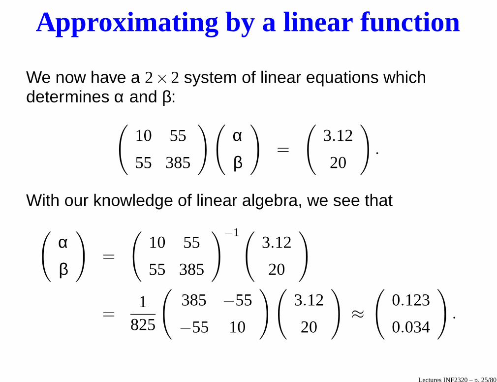
We now have a 2×2 system of linear equations whichdetermines α and β:
(
10 55
55 385
)(
αβ
)
=
(
3.12
20
)
.
With our knowledge of linear algebra, we see that
(
αβ
)
=
(
10 55
55 385
)−1(3.12
20
)
=1
825
(
385 −55
−55 10
)(
3.12
20
)
≈
(
0.123
0.034
)
.
Lectures INF2320 – p. 25/80
Approximating by a linear function
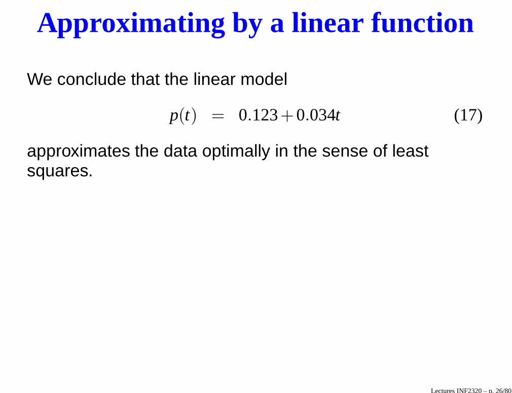
We conclude that the linear model
p(t) = 0.123+0.034t (17)
approximates the data optimally in the sense of leastsquares.
Lectures INF2320 – p. 26/80

1991 1992 1993 1994 1995 1996 1997 1998 1999 20000
0.1
0.2
0.3
0.4
0.5
0.6
0.7
Figure 9: Constant and linear least squares approximations of
the global annual mean temperature deviation measurements from
year 1991 to 2000.Lectures INF2320 – p. 27/80

Approx. by a quadratic function
• We now want to determine constants α, β and γ, suchthat the quadratic polynomial
p(t) = α+βt + γt2 (18)
fits the data optimally in the sense of least squares• Minimizing
F(α,β,γ) =10
∑i=1
(α+βti + γt2i − yi)
2 (19)
requires
∂F∂α
=∂F∂β
=∂F∂γ
= 0 (20)
Lectures INF2320 – p. 28/80
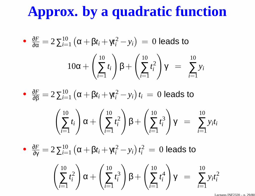
Approx. by a quadratic function
• ∂F∂α = 2∑10
i=1
(
α+βti + γt2i − yi
)
= 0 leads to
10α+
(
10
∑i=1
ti
)
β+
(
10
∑i=1
t2i
)
γ =10
∑i=1
yi
• ∂F∂β = 2∑10
i=1
(
α+βti + γt2i − yi
)
ti = 0 leads to(
10
∑i=1
ti
)
α+
(
10
∑i=1
t2i
)
β+
(
10
∑i=1
t3i
)
γ =10
∑i=1
yiti
• ∂F∂γ = 2∑10
i=1
(
α+βti + γt2i − yi
)
t2i = 0 leads to
(
10
∑i=1
t2i
)
α+
(
10
∑i=1
t3i
)
β+
(
10
∑i=1
t4i
)
γ =10
∑i=1
yit2i
Lectures INF2320 – p. 29/80
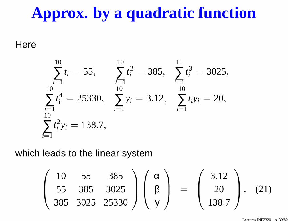
Approx. by a quadratic function
Here
10
∑i=1
ti = 55,10
∑i=1
t2i = 385,
10
∑i=1
t3i = 3025,
10
∑i=1
t4i = 25330,
10
∑i=1
yi = 3.12,10
∑i=1
tiyi = 20,
10
∑i=1
t2i yi = 138.7,
which leads to the linear system
10 55 38555 385 3025385 3025 25330
αβγ
=
3.1220
138.7
. (21)
Lectures INF2320 – p. 30/80
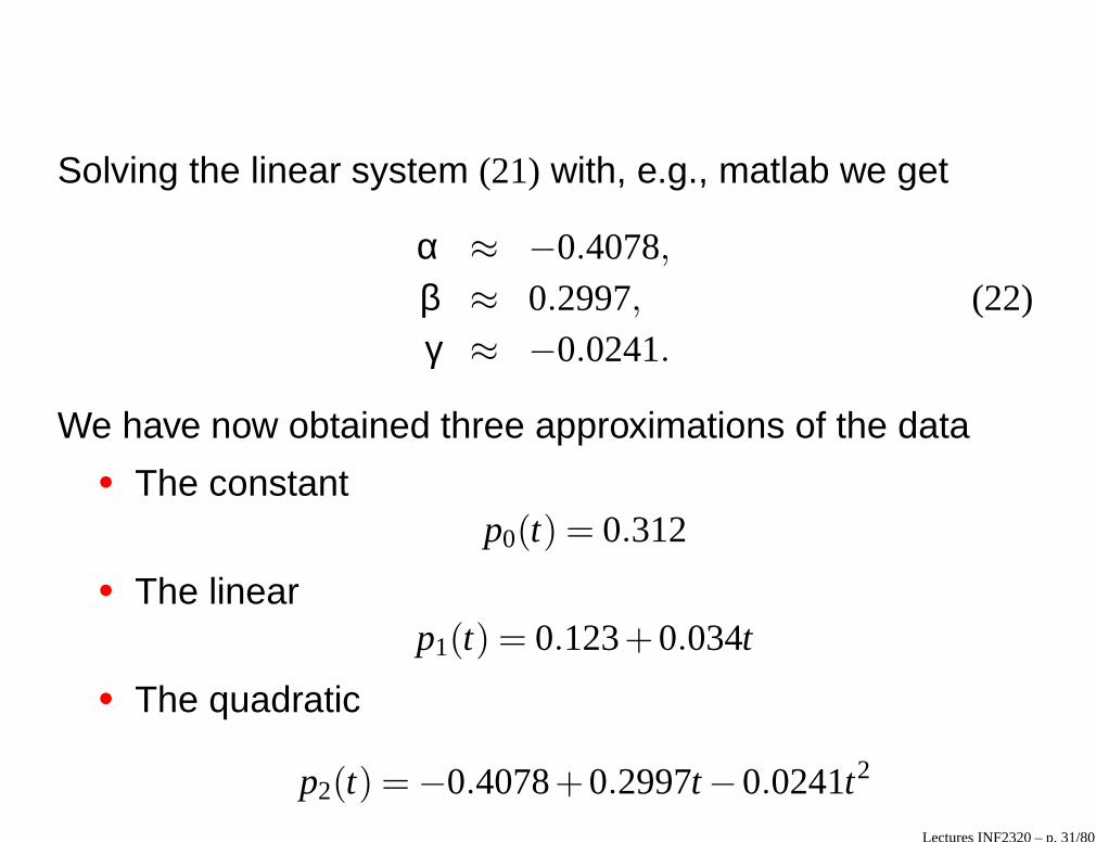
Solving the linear system (21) with, e.g., matlab we get
α ≈ −0.4078,β ≈ 0.2997, (22)γ ≈ −0.0241.
We have now obtained three approximations of the data• The constant
p0(t) = 0.312
• The linearp1(t) = 0.123+0.034t
• The quadratic
p2(t) = −0.4078+0.2997t −0.0241t2
Lectures INF2320 – p. 31/80
1991 1992 1993 1994 1995 1996 1997 1998 1999 20000
0.1
0.2
0.3
0.4
0.5
0.6
0.7
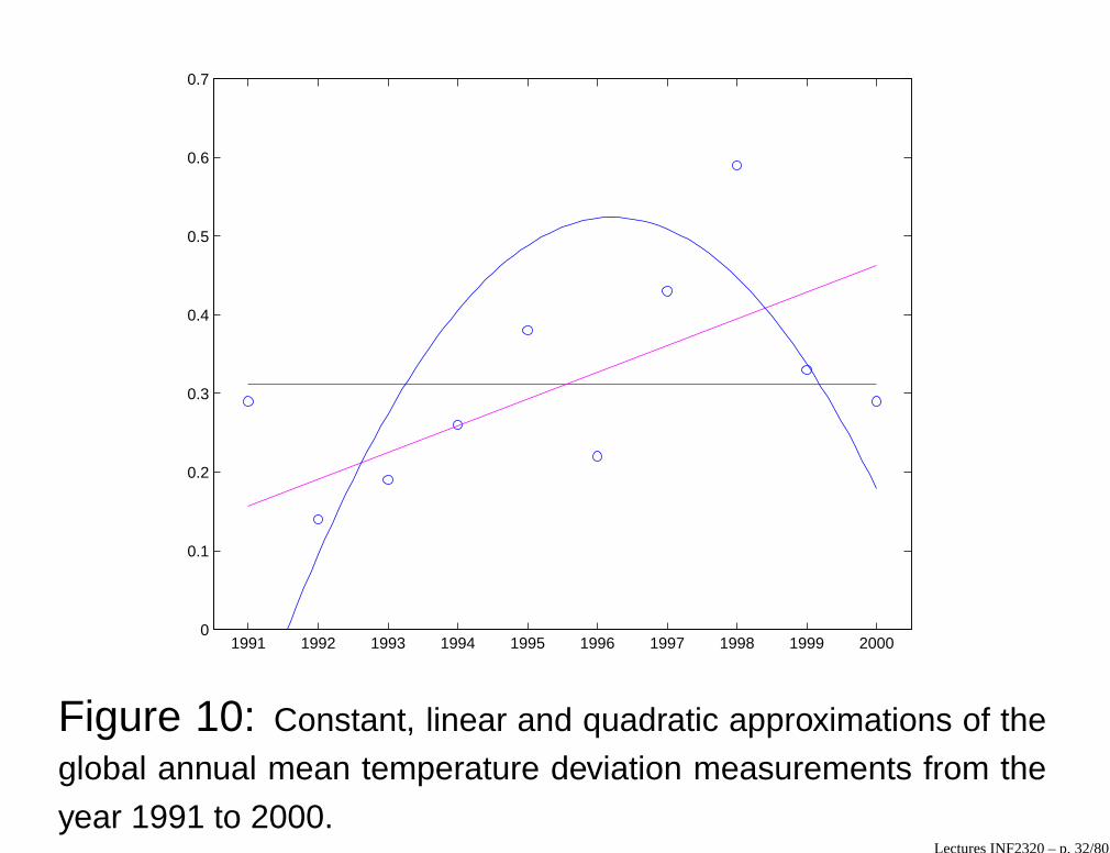
Figure 10: Constant, linear and quadratic approximations of the
global annual mean temperature deviation measurements from the
year 1991 to 2000.Lectures INF2320 – p. 32/80
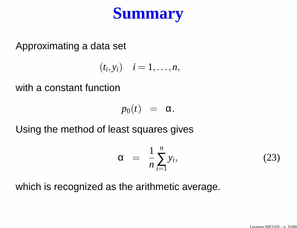
Summary
Approximating a data set
(ti,yi) i = 1, . . . ,n,
with a constant function
p0(t) = α.
Using the method of least squares gives
α =1n
n
∑i=1
yi, (23)
which is recognized as the arithmetic average.
Lectures INF2320 – p. 33/80

Summary
Approximating the data set with a linear function
p1(t) = α+βt
can be done by minimizing
minα,β
F(α,β) = minα,β
n
∑i=1
(p1(ti)− yi)2,
which leads to the following 2×2 linear system
nn
∑i=1
ti
n
∑i=1
tin
∑i=1
t2i
α
β
=
n
∑i=1
yi
n
∑i=1
tiyi
. (24)
Lectures INF2320 – p. 34/80

Summary
A quadratic approximation on the form
p2(t) = α+βt + γt2
can be done by minimizingminα,β,γ F(α,β,γ) = minα,β,γ ∑n
i=1(p2(ti)− yi)2, which leads to
the following 3×3 linear system
nn
∑i=1
tin
∑i=1
t2i
n
∑i=1
tin
∑i=1
t2i
n
∑i=1
t3i
n
∑i=1
t2i
n
∑i=1
t3i
n
∑i=1
t4i
αβγ
=
n
∑i=1
yi
n
∑i=1
yiti
n
∑i=1
yit2i
. (25)
Lectures INF2320 – p. 35/80

Large Data Sets
1850 1900 1950 2000−0.6
−0.4
−0.2
0
0.2
0.4
0.6
Figure 11: The global annual mean temperature deviation mea-
surements from the year 1856 to 2000.
Lectures INF2320 – p. 36/80
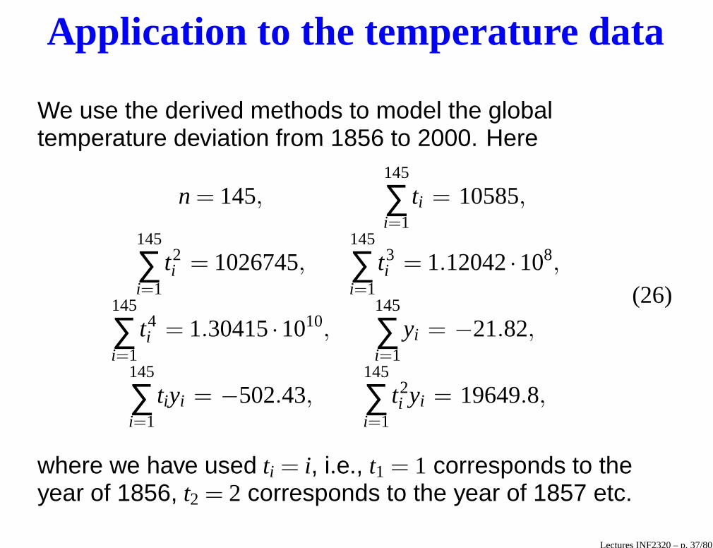
Application to the temperature data
We use the derived methods to model the globaltemperature deviation from 1856 to 2000. Here
n = 145,145
∑i=1
ti = 10585,
145
∑i=1
t2i = 1026745,
145
∑i=1
t3i = 1.12042·108,
145
∑i=1
t4i = 1.30415·1010,
145
∑i=1
yi = −21.82,
145
∑i=1
tiyi = −502.43,145
∑i=1
t2i yi = 19649.8,
(26)
where we have used ti = i, i.e., t1 = 1 corresponds to theyear of 1856, t2 = 2 corresponds to the year of 1857 etc.
Lectures INF2320 – p. 37/80

Application to the temperature data
First we get the constant model
p0(t) ≈ −0.1505. (27)
The coefficients α and β of the linear model are obtained bysolving the linear system (24), i.e.
(
145 1058510585 1026745
)(
αβ
)
=
(
−21.82−502.43
)
.
Consequently,
α ≈ −0.4638 and β ≈ 0.0043,
so the linear model is given by
p1(t) ≈ −0.4638+0.0043t. Lectures INF2320 – p. 38/80

Application to the temperature data
Similarly, the coefficients α, β and γ of the quadratic modelare obtained by solving the linear system (25), i.e.
145 10585 1026745·106
10585 1026745·106 1.12042·108
1026745·106 1.12042·108 1.30415·1010
αβγ
=
−21.82−502.4319649.8
.
The solution of this system is given by
α ≈ −0.3136, β ≈ −1.8404·10−3 and γ ≈ 4.2005·10−5,
so the quadratic model is given by
p2(t) ≈ −0.3136−1.8404·10−3t +4.2005·10−5t2. (28)
Lectures INF2320 – p. 39/80

1850 1900 1950 2000−0.6
−0.4
−0.2
0
0.2
0.4
0.6
Figure 12: Constant, linear and quadratic least squares approxi-
mations of the global annual mean temperature deviation measure-
ments; from 1856 to 2000.Lectures INF2320 – p. 40/80

Application to population models
We now consider the growth of the world population.
Year Population (billions)
1950 2.555
1951 2.593
1952 2.635
1953 2.680
1954 2.728
1955 2.780
Table 2: The total world population from 1950 to 1955.
Lectures INF2320 – p. 41/80

Exponential growth
First we model the data in Table 2 using the exponentialgrowth model
p′(t) = αp(t), p(0) = p0, (29)
with solution p(t) = p0eαt .• We have earlier mentioned that for this model α has to
be estimated• We shall now estimate α relative to this data, in the
sense of least squares
Lectures INF2320 – p. 42/80
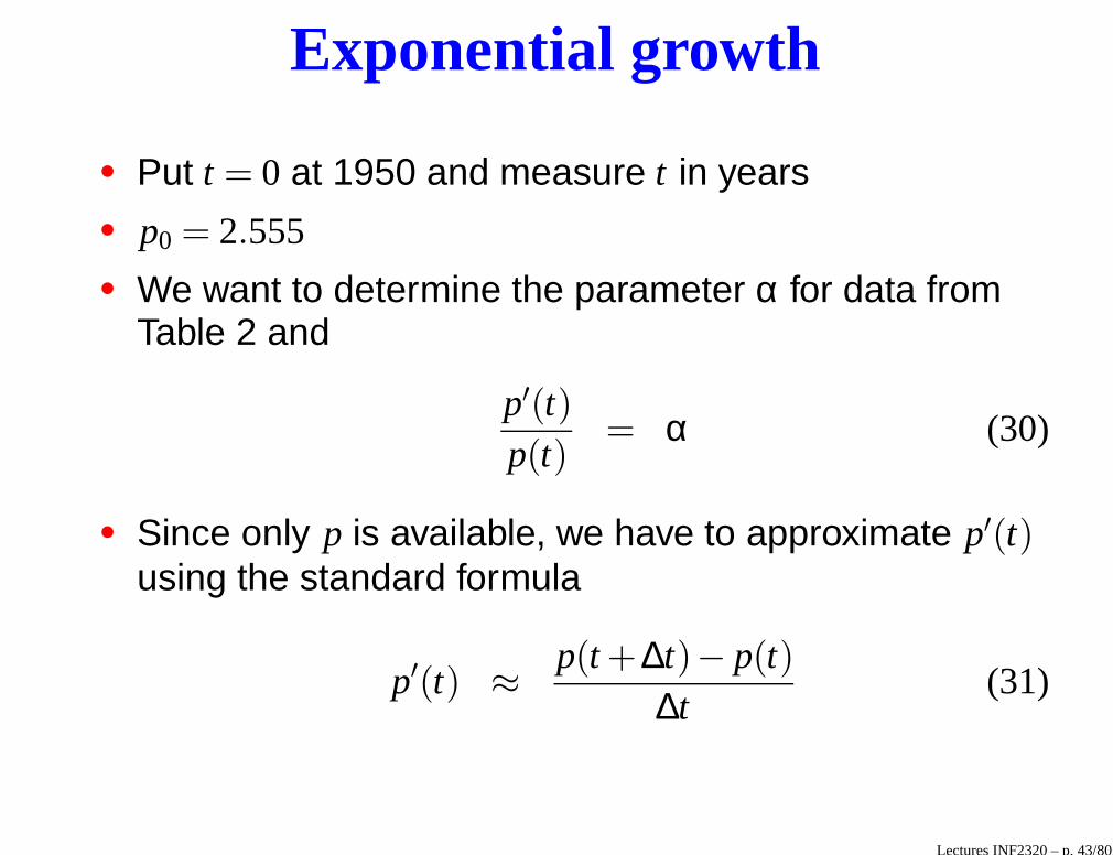
Exponential growth
• Put t = 0 at 1950 and measure t in years• p0 = 2.555
• We want to determine the parameter α for data fromTable 2 and
p′(t)p(t)
= α (30)
• Since only p is available, we have to approximate p′(t)using the standard formula
p′(t) ≈p(t +∆t)− p(t)
∆t(31)
Lectures INF2320 – p. 43/80
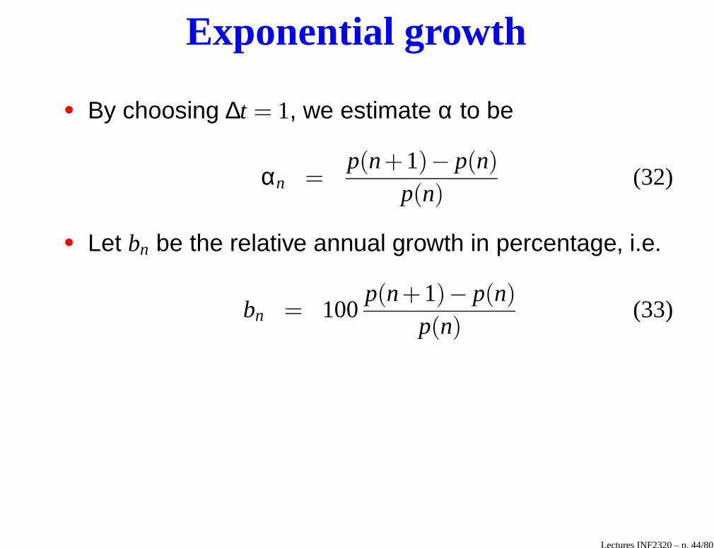
Exponential growth
• By choosing ∆t = 1, we estimate α to be
αn =p(n+1)− p(n)
p(n)(32)
• Let bn be the relative annual growth in percentage, i.e.
bn = 100p(n+1)− p(n)
p(n)(33)
Lectures INF2320 – p. 44/80
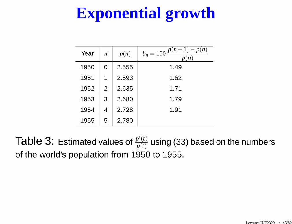
Exponential growth
Year n p(n) bn = 100p(n+1)− p(n)
p(n)
1950 0 2.555 1.49
1951 1 2.593 1.62
1952 2 2.635 1.71
1953 3 2.680 1.79
1954 4 2.728 1.91
1955 5 2.780
Table 3: Estimated values of p′(t)p(t) using (33) based on the numbers
of the world’s population from 1950 to 1955.
Lectures INF2320 – p. 45/80

Exponential growth
• We can to compute a constant approximation b, to thisdata set in the sense of least squares, i.e. the average
b =15
4
∑n=0
bn =15(1.49+1.62+1.71+1.79+1.91) = 1.704
• Since bn = 100αn we get
α =1
100b = 0.01704 (34)
• This gives us the model
p(t) = 2.555e0.01704t (35)
Lectures INF2320 – p. 46/80

Exponential growth
• In the year 2000 (t=50) this model gives
p(50) = 2.555e0.01704×50≈ 5.990 (36)
• The actual population in the 2000 was 6.080 billions• The relative error is
6.080−5.9906.080
·100% = 1.48%, (37)
which is remarkably small
Lectures INF2320 – p. 47/80

1950 1955 1960 1965 1970 1975 1980 1985 1990 1995 20002.5
3
3.5
4
4.5
5
5.5
6
6.5x 10
9
Figure 13: The figure shows the graph of an exponential popu-
lation model p(t) = 2.555e0.01704t together with the actual measure-
ments marked by ’o’.Lectures INF2320 – p. 48/80

Exponential growth
• Will this model fit in the future as well?• We try to use the development from 1990 to 2000 (see
Figure 13) to predict the world population in 2100
Lectures INF2320 – p. 49/80

Year n p(n) bn = 100 p(n+1)−p(n)p(n)
1990 0 5.284 1.57
1991 1 5.367 1.55
1992 2 5.450 1.49
1993 3 5.531 1.46
1994 4 5.611 1.43
1995 5 5.691 1.37
1996 6 5.769 1.35
1997 7 5.847 1.33
1998 8 5.925 1.32
1999 9 6.003 1.28
2000 10 6.080
Table 4: The calculated bn values associated with an exponential
population model for the world between 1990 and 2000.
Lectures INF2320 – p. 50/80

Exponential growth
• The average of the bn values is
b =110
9
∑n=0
bn = 1.42
• Therefore α = b100 = 0.0142
• Starting from t=0 in the year 2000, the model reads
p(t) = 6.080e0.0142t (38)
• This model predicts that there will be
p(100) = 6.080e1.42≈ 25.2 (39)
billion people living on the earth in the year of 2100
Lectures INF2320 – p. 51/80

Logistic growth of the world pop.
• We study how the world population can be modeled bythe logistic growth model
p′(t) = α p(t)(1− p(t)/β) (40)
• By defining γ = −α/β, we can rewrite (40)
p′(t)p(t)
= α+ γ p(t) (41)
• Hence, we can determine constants α and γ by fitting alinear function to the observations of
p′(t)p(t)
(42)
Lectures INF2320 – p. 52/80

Logistic growth
• As above we define
bn = 100p(n+1)− p(n)
p(n)(43)
• We now want to determine two constants A and B,such that the data are modeled as accurately aspossible by a linear function
bn ≈ A+Bp(n), (44)
in the sense of least squares
Lectures INF2320 – p. 53/80

Logistic growth
• A and B can be determined by the following 2×2 linearsystem,
109
∑n=0
p(n)
9
∑n=0
p(n)9
∑n=0
(p(n))2
A
B
=
9
∑n=0
bn
9
∑n=0
p(n)bn
(45)
• We have9
∑n=0
p(n) = 56.5,9
∑n=0
(p(n))2 = 319.5,
9
∑n=0
bn ≈ 14.1,9
∑n=0
p(n)bn ≈ 79.6
Lectures INF2320 – p. 54/80

Logistic growth
• By solving the (2×2) system(
10 56.556.5 319.5
)(
AB
)
=
(
14.179.6
)
we get
A = 2.7455 and B = −0.2364
• Inserting this in the logistic model we get
p′(t) ≈ 0.027p(t)(1− p(t)/11.44) (46)
• This indicates that the carrying capacity of the earth isabout 11.44 billions
Lectures INF2320 – p. 55/80

Logistic growth
• Let t = 0 correspond to the year 2000, which gives theinitial condition
p(0) ≈ 6.08
• The analytical solution to the differential equation is
p(t) ≈69.5
6.08+5.36e−0.027t(47)
• This model predicts that there will be
p(100) ≈ 10.79
billion people on the earth in the year of 2100
Lectures INF2320 – p. 56/80

2000 2010 2020 2030 2040 2050 2060 2070 2080 2090 21000.6
0.8
1
1.2
1.4
1.6
1.8
2
2.2
2.4
2.6x 10
10
Figure 14: Predictions of the population growth on the earth
based on an exponential model (solid curve) and a logistic model
(dashed curve).Lectures INF2320 – p. 57/80

Approximations of Functions
• Above we have studied continuous representation ofdiscrete data
• Next we will consider continuous approximation ofcontinuous functions
• Consider the function
y(t) = ln
(
110
sin(t)+ et
)
(48)
• In Figure 15 we see that y(x) seems to be close to thelinear function p(t) = t on the interval [0,1]
• In Figure 16 we see that y(x) seems to be even closerto the linear function plotted on t ∈ [0,10]
Lectures INF2320 – p. 58/80

0 0.1 0.2 0.3 0.4 0.5 0.6 0.7 0.8 0.9 10
0.2
0.4
0.6
0.8
1
1.2
Figure 15: The function y(t) = ln(
110 sin(t)+ et
)
(solid curve) and
a linear approximation (dashed line) on the interval t ∈ [0,1].
Lectures INF2320 – p. 59/80

0 1 2 3 4 5 6 7 8 9 100
1
2
3
4
5
6
7
8
9
10
Figure 16: The function y(t) = ln(
110 sin(t)+ et
)
(solid curve) and
a linear approximation (dashed line) on the interval t ∈ [0,10].
Lectures INF2320 – p. 60/80

Approximations by constants
• For a given function y(t), t ∈ [a,b], we want to computea constant approximation of it
p(t) = α (49)
for t ∈ [a,b], in the sense of least squares• That means that we want to minimize the integral
∫ b
a(p(t)− y(t))2 dt =
∫ b
a(α− y(t))2 dt
Lectures INF2320 – p. 61/80

Approximations by constants
• Define the function
F(α) =∫ b
a(α− y(t))2 dt (50)
• The derivative with respect to α is
F ′(α) = 2∫ b
a(α− y(t)) dt
• And solving F ′(α) = 0 gives
α =1
b−a
∫ b
ay(t)dt (51)
Lectures INF2320 – p. 62/80
Note that
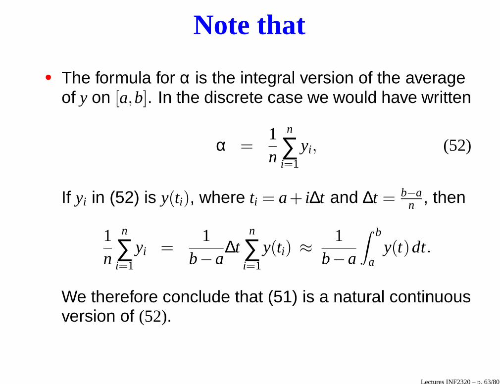
• The formula for α is the integral version of the averageof y on [a,b]. In the discrete case we would have written
α =1n
n
∑i=1
yi, (52)
If yi in (52) is y(ti), where ti = a+ i∆t and ∆t = b−an , then
1n
n
∑i=1
yi =1
b−a∆t
n
∑i=1
y(ti) ≈1
b−a
∫ b
ay(t)dt.
We therefore conclude that (51) is a natural continuousversion of (52).
Lectures INF2320 – p. 63/80

Note that
• We used
ddα
∫ b
a(α− y(t))2dt =
∫ b
a
∂∂α
(α− y(t))2dt
Is that a legal operation? This is discussed inExercise 5.
• The α given by (51) is a minimum, since
F ′′(α) = 2(b−a) > 0
Lectures INF2320 – p. 64/80
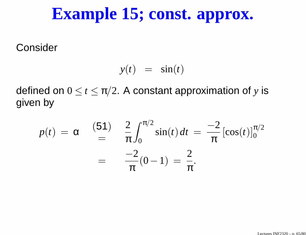
Example 15; const. approx.
Consider
y(t) = sin(t)
defined on 0≤ t ≤ π/2. A constant approximation of y isgiven by
p(t) = α (51)=
2π
∫ π/2
0sin(t)dt =
−2π
[cos(t)]π/20
=−2π
(0−1) =2π.
Lectures INF2320 – p. 65/80

Example 16; const. approx.
Consider
y(t) = t2 +110
cos(t)
defined on 0≤ t ≤ 1. A constant approximation of y is givenby
p(t) = α (51)=
∫ 1
0
(
t2 +110
cos(t)
)
dt =
[
13
t3 +110
sin(t)
]1
0
=13
+110
sin(1) ≈ 0.417.
Lectures INF2320 – p. 66/80
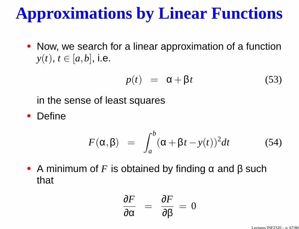
Approximations by Linear Functions
• Now, we search for a linear approximation of a functiony(t), t ∈ [a,b], i.e.
p(t) = α+β t (53)
in the sense of least squares• Define
F(α,β) =
∫ b
a(α+β t − y(t))2dt (54)
• A minimum of F is obtained by finding α and β suchthat
∂F∂α
=∂F∂β
= 0
Lectures INF2320 – p. 67/80
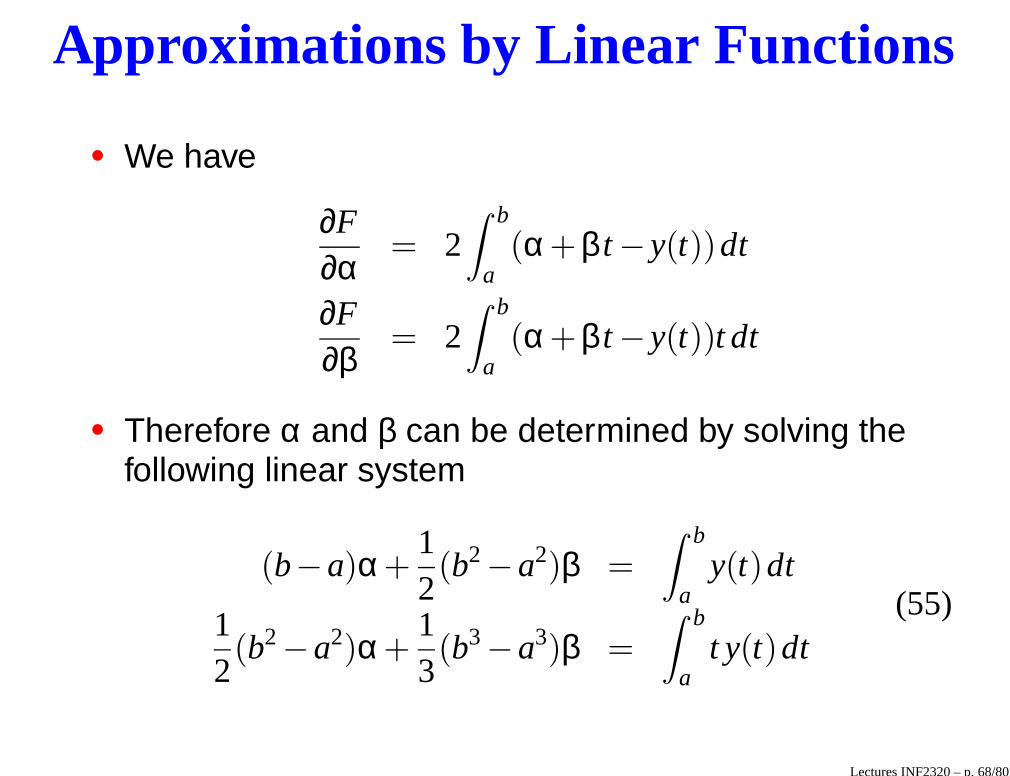
Approximations by Linear Functions
• We have
∂F∂α
= 2∫ b
a(α+β t − y(t))dt
∂F∂β
= 2∫ b
a(α+β t − y(t))t dt
• Therefore α and β can be determined by solving thefollowing linear system
(b−a)α+12(b2
−a2)β =∫ b
ay(t)dt
12(b2
−a2)α+13(b3
−a3)β =
∫ b
at y(t)dt
(55)
Lectures INF2320 – p. 68/80

Example 15; linear approx.
Consider
y(t) = sin(t)
defined on 0≤ t ≤ π/2.We have
∫ π/2
0sin(t)dt = 1
and∫ π/2
0t sin(t)dt = 1.
Lectures INF2320 – p. 69/80

Example 15; linear approx.
The linear system now reads(
π/2 π2/8π2/8 π3/24
)(
αβ
)
=
(
11
)
.
The solution is
(
αβ
)
=1π2
8π−2496π
−24
≈
(
0.1150.664
)
.
Therefore the linear approximation is given by
p(t) ≈ 0.115+0.664t.
Lectures INF2320 – p. 70/80
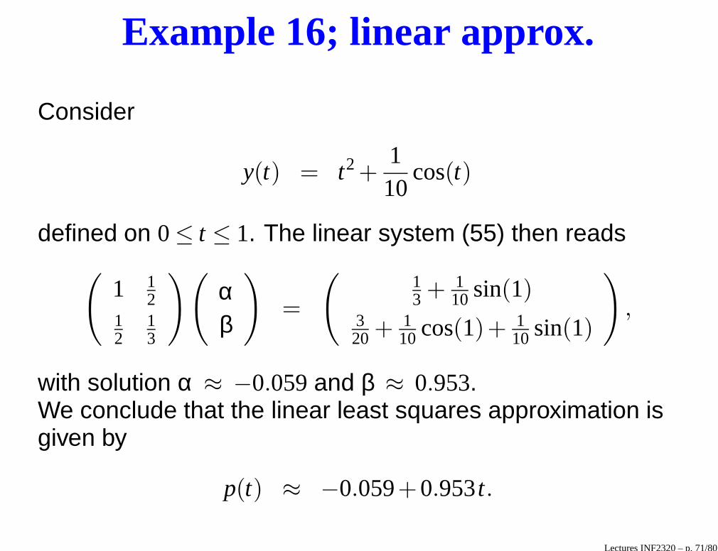
Example 16; linear approx.
Consider
y(t) = t2 +110
cos(t)
defined on 0≤ t ≤ 1. The linear system (55) then reads(
1 12
12
13
)(
αβ
)
=
(
13 + 1
10 sin(1)320 + 1
10 cos(1)+ 110 sin(1)
)
,
with solution α ≈ −0.059and β ≈ 0.953.We conclude that the linear least squares approximation isgiven by
p(t) ≈ −0.059+0.953t.
Lectures INF2320 – p. 71/80
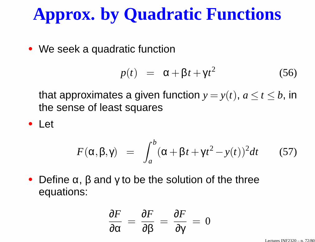
Approx. by Quadratic Functions
• We seek a quadratic function
p(t) = α+β t + γ t2 (56)
that approximates a given function y = y(t), a ≤ t ≤ b, inthe sense of least squares
• Let
F(α,β,γ) =
∫ b
a(α+β t + γ t2
− y(t))2dt (57)
• Define α, β and γ to be the solution of the threeequations:
∂F∂α
=∂F∂β
=∂F∂γ
= 0
Lectures INF2320 – p. 72/80

Approx. by Quadratic Functions
• By taking the derivatives, we have•
∂F∂α
= 2∫ b
a(α+β t + γ t2
− y(t))dt
•
∂F∂β
= 2∫ b
a(α+β t + γ t2
− y(t)) t dt
•
∂F∂γ
= 2∫ b
a(α+β t + γ t2
− y(t)) t2dt
Lectures INF2320 – p. 73/80
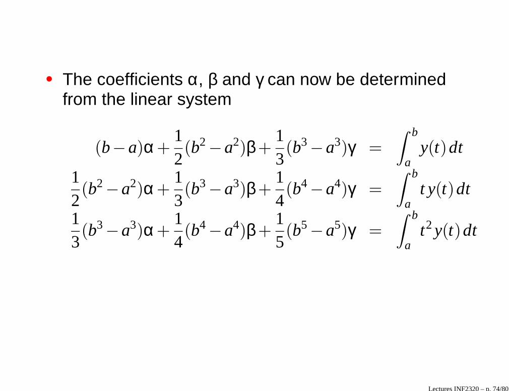
• The coefficients α, β and γ can now be determinedfrom the linear system
(b−a)α+12(b2
−a2)β+13(b3
−a3)γ =
∫ b
ay(t)dt
12(b2
−a2)α+13(b3
−a3)β+14(b4
−a4)γ =∫ b
at y(t)dt
13(b3
−a3)α+14(b4
−a4)β+15(b5
−a5)γ =
∫ b
at2y(t)dt
Lectures INF2320 – p. 74/80

Example 15; quad. approx.
For the function
y(t) = sin(t), 0≤ t ≤ π/2,
the linear system reads
π/2 π2/8 π3/24π2/8 π3/24 π4/64
π3/24 π4/64 π5/160
αβγ
=
11
π−2
,
and the solution is given by α ≈ −0.024, β ≈ 1.196andγ ≈ −0.338, which gives the quadratic approximation
p(t) = −0.024+1.196t −0.338t2.
Lectures INF2320 – p. 75/80

Example 16; quad. approx.
Let us consider
y(t) = t2 +110
cos(t)
for 0≤ t ≤ 1. The linear system takes the form
1 1/2 1/31/2 1/3 1/41/3 1/4 1/5
αβγ
=
13 + 1
10 sin(1)320 + 1
10 cos(1)+ 110 sin(1)
15 + 1
5 cos(1)− 110 sin(1)
and the solution is given by α ≈ 0.100, β ≈ −0.004andγ ≈ 0.957, and the quadratic approximation is
p(t) = 0.100−0.004t +0.957t2.
Lectures INF2320 – p. 76/80

0 0.5 1 1.5
0
0.2
0.4
0.6
0.8
1
Figure 17: The function y(t) = sin(t) (solid curve) and its least
squares approximations: constant (dashed line), linear (dotted line)
and quadratic (dashed-dotted curve).Lectures INF2320 – p. 77/80
0 0.1 0.2 0.3 0.4 0.5 0.6 0.7 0.8 0.9 1
0
0.1
0.2
0.3
0.4
0.5
0.6
0.7
0.8
0.9
1
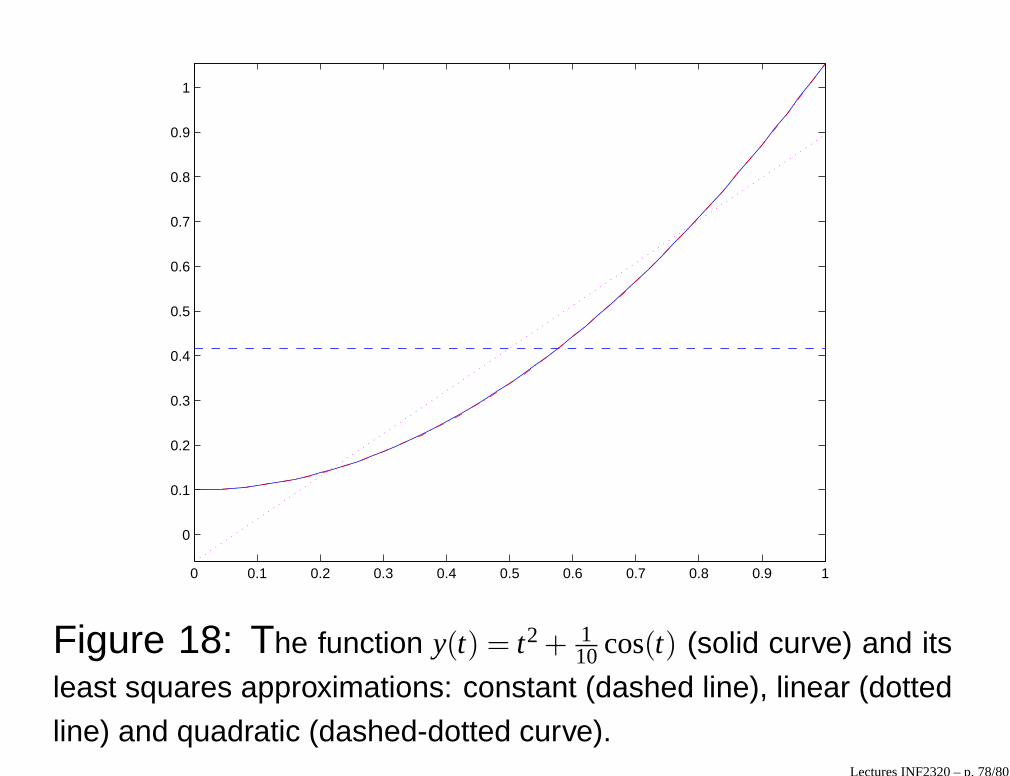
Figure 18: The function y(t) = t2 + 110 cos(t) (solid curve) and its
least squares approximations: constant (dashed line), linear (dotted
line) and quadratic (dashed-dotted curve).Lectures INF2320 – p. 78/80

Lectures INF2320 – p. 79/80

Lectures INF2320 – p. 80/80