THE MEASUREMENT OF AGGREGATE TOTAL FACTOR PRODUCTIVITY GROWTH*

(November 18, 2002)

W. Erwin Diewert Alice O. Nakamura Department of Economics Faculty of Business, University of Alberta University of British Columbia Edmonton, Alberta T6G 2R6 Vancouver, British Columbia V6T 1W5 e-mail: alice.nakamura@ualberta.ca e-mail: diewert@econ.ubc.ca 1. INTRODUCTION 1

2. ALTERNATIVE CONCEPTS AND PERSPECTIVES FOR PRODUCTIVITY MEASUREMENT 5 3. FOUR TFPG MEASURES FOR THE N-M CASE 10 4. THE AXIOMATIC (OR TEST) APPROACH TO CHOOSING AMONG ALTERNATIVE INDEX NUMBER FORMULAS 18 5. THE EXACT INDEX NUMBER APPROACH AND SUPERLATIVE INDEX NUMBERS 20 6. PRODUCTION FUNCTION BASED MEASURES OF TFPG 27 7. COST FUNCTION BASED MEASURES 38 8. THE DIEWERT-MORRISON PRODUCTIVITY MEASURE AND DECOMPOSITIONS 43 9. THE DIVISIA APPROACH 47 10. GROWTH ACCOUNTING 54 11. CONCLUSIONS 60 REFERENCES 65

*This research was funded by the grants from the Social Sciences and Humanities Research Council of Canada (SSHRC). Thanks are due to Jim Heckman, Rosa Matzkin, Amil Petrin, Arnold Zellner, Richard Blundell and other participants in the Handbook of Econometrics, Volume 6 Conference held at the University of Chicago, November 17, 2001; to the participants in a December, 2000 London Handbook of Econometrics Workshop; to Bo Honoré and other participants in a Princeton seminar; and to John Baldwin, Mel Fuss, David Laidler, Denis Lawrence, Richard Lipsey, Emi Nakamura, Masao Nakamura, Someshwar Rao, and Tom Wilson as well as other participants in a workshop held at Statistics Canada on October 25-26, 2001 with funding from our SSHRC grants. The authors also thank the participants in a June 15-17, 2000 Union College workshop for comments on the paper given there by Erwin Diewert that was the starting point for this chapter. All errors are the sole responsibility of the authors. The authors can be reached at the e-mail addresses <diewert@econ.ubc.ca> and <alice.nakamura@ualberta.ca>. Their mailing addresses are Professor W. Erwin Diewert, 1873 East Mall, Buchanan Tower, room 997, Department of Economics, University of British Columbia, Vancouver, Canada, V6T 1Z1 and Professor Alice O. Nakamura, Faculty of Business, University of Alberta, Edmonton, Canada, T6G 2R. This chapter is forthcoming in the Elsevier Science Handbook of Econometrics, Volume 6, edited by J. J. Heckman and E. E. Leamer.

ABSTRACT FOR THE CHAPTER JEL Classification Codes: O4 Economic growth and aggregate productivity O4.7 Measurement of economic growth; aggregate productivity This chapter surveys the theory and methods of the measurement of aggregate productivity as characterized by total factor productivity (TFP) and total factor productivity growth (TFPG). Index number methods are the mainstay methodology for estimating national productivity. Different conceptual meanings have been proposed for a TFPG index. The alternative concepts are easiest to understand for the case in which the index number problem is absent: a production process with one input and one output (a 1-1 process). We show that four common concepts of TFPG all lead to the same measure in this 1-1 case. However, with only 1 input and one output it is not possible to introduce aggregation issues. To do that, we move on to a production process with two inputs (a 2-1 process). After that we present several of the commonly used index number formulas for a general N input, M output production scenario. One result demonstrated is that a Paasche, Laspeyres or Fisher index number formula provides a measure for all of the four concepts of TFPG introduced for the 1-1 case. Nevertheless, with multiple inputs and outputs, different formula choices lead to different TFPG measures. This raises the issue of choice among alternative TFPG formulas. One approach to this problem is to use algebra and economic theory restrictions to establish that certain index number formulas correspond, by Diewert’s “exact” index number approach, to linearly homogeneous producer behavioral relationships that are “flexible” in the sense defined by Diewert that they provide a second order approximation to an arbitrary twice continuously differentiable linearly homogeneous function. Diewert coined the term “superlative” for an index number functional form that is exact for a behavioral relationship with a functional form that is flexible. When the exact index number approach and Diewert’s numerical analysis approximation results for superlative index numbers are applied, the a priori information requirements for choosing an index number formula are reduced to a list of general characteristics of the production scenario. Additional topics discussed in this chapter include an alternative family of theoretical productivity growth indexes proposed by Diewert and Morrison, the Divisia method, and growth accounting.

1

1. INTRODUCTION

“Implementing a strategy to achieve a higher standard of living for all Canadians always comes back to dealing squarely with the same deeply-rooted challenge: enhancing Canada’s long-term productivity.”

(The Honourable Jean Chrétien Prime Minister of Canada

Confederation Dinner, October 26, 1998) “The two main sources of economic growth in output are increases in the factors of production (the labour and capital devoted to production) and efficiency or productivity gains that enable an economy to produce more for the same amount of inputs.”

(Baldwin, Harchaoui, Hosein and Maynard, 2000 “Productivity: Concepts and Trends”

Statistics Canada) “Productivity is commonly defined as a ratio of a volume measure of output to a volume measure of input use. While there is no disagreement on this general notion, a look at the productivity literature and its various applications reveals very quickly that there is neither a unique purpose for nor a single measure of productivity.”

(Paul Schreyer OECD Statistics Directorate

OECD PRODUCTIVITY MANUAL, 2001)

Productivity is like love. Much is said about the benefits of having more of it, but disagreement reigns on how best to achieve this. One reason for this is a lack of consensus on what “it” really is. Many economists are also unfamiliar with the methods that are used for measuring aggregate productivity, by which we mean the productivity of unique entities such as nations or entire industries. National productivity estimates are of special importance because they are an input into many aspects of public policy making.1 At this level of aggregation, the data available are limited to fairly short time series, putting bounds on the scope for econometric estimation. As a consequence, index number methods (including growth accounting) are the mainstay methodology. This chapter surveys the index number theory and methods for the

1 For instance, the national monetary authorities for countries such as Canada routinely consider national TFPG estimates in making decisions about acceptable amounts of price inflation. National productivity estimates and inter-country comparisons of these are cited in debates concerning a wide range of public policy issues. The release of productivity figures by national statistical agencies is often front page news. National public policy issues are given as one motivation for many of the studies of productivity including Aschauer (1989), Baily (1981), Balk (1996), Basu and Fernald (1997), Bernard and Jones (1996), Berndt and Khaled (1979), Black and Lynch (1996), Boskin (1997), Bruno and Sachs (1982), Crawford (1993), Denison (1979), Diewert (2001), Diewert and Fox (1999), Diewert and Lawrence (1995), Griliches (1997), Hulten (1986, 2001), Jorgensen and Lee (2001), Maddison (1987), Muellbauer (1986), Nadiri (1980), Nordhaus (1982), Odagiri (1985), Power (1998), Prescott (1998), and Wolff (1985, 1996, 1997).

2

measurement of aggregate productivity as characterized by total factor productivity (TFP) and total factor productivity growth (TFPG). The traditional index number measures of TFPG are defined as ratios of output and input quantity indexes. A TFP growth estimate does not, by itself, tell us anything about what caused this growth just as the annual values for the nominal or the real revenue/cost ratio for a business do not, by themselves, tell us why profitability has been rising or falling. Nevertheless, just as many aspects of business planning are affected by information about whether revenues have been rising faster or more slowly than costs, likewise, estimates of national productivity growth affect national economic policies. It is important for these estimates to be accurate and understood. Also, in order to explore explanations for TFP growth, it is first necessary to measure it.2 For economists there are other reasons as well why it is important to have a good understanding of index numbers. The quantity and price index components of the traditional TFPG indexes are used for a wide range of purposes in applied econometric studies. For example, monetary variables in studies making use of observations over time are typically deflated using price indexes. In this chapter, we review the definitions of the Laspeyres, Paasche, Fisher, Törnqvist, and implicit Törnqvist quantity and price indexes and the corresponding TFPG indexes. Several different conceptual meanings have been proposed for a TFPG index. The alternative concepts are easiest to understand for a one period production process that uses a single input factor to make a single output good (what we refer to as a 1-1 process). In section 2 we show that four common concepts of TFPG all lead to the same measure in the 1-1 case. Of course, the aggregation challenges that must be confronted in the construction of index numbers cannot be introduced in a 1-1 case context because they do not arise. Thus, in section 2 we also use a hypothetical two input, one output production scenario (that is, a 2-1 process) as a context for briefly introducing and motivating some of the choices faced in forming quantity aggregates, quantity indexes and TFPG indexes when there are multiple inputs or outputs. For a general N input, M output production scenario, the inputs and the outputs must be aggregated. If price weights are used for this purpose, then issues of price change must be dealt with too. In section 3, we define aggregates and quantity and price indexes that are components of the TFPG indexes. One important result demonstrated in this section is that, for several of the commonly used functional forms, the resulting TFPG formula can be viewed as a measure for all 2 For gaining a causal understanding of the ups and downs of national productivity, data at lower levels of aggregation are of great value. While beyond the scope of this survey, studies based on micro level evidence that represent important advances in understanding productivity growth include Bartelsman and Doms (2000); Blundell, Griffith and Van Reenen (1999); Cockburn, Henderson and Stern (2000); Foster, Krizan and Haltiwanger (1998); Levinsohn and Petrin (1999); Olley and Pakes (1996); and Pavcnik (2001).

3

of the four distinct concepts of TFPG introduced in section 2. Nevertheless, with multiple inputs and outputs, different formula choices lead to different TFPG measures. This raises the issue of choice among alternative TFPG formulas. The two main approaches to choosing among the different index number functional forms are the axiomatic (or test) approach and the exact approach also referred to as an economic approach. The axiomatic approach is taken up in section 4. It was used extensively by the founding contributors to index number theory, including Fisher (1911, 1922). This approach makes use of lists of desired properties for price, quantity, or productivity indexes. These properties are referred to as axioms or tests. They are either formalizations of common sense properties of good index numbers or generalizations of properties that hold for virtually all proposed index number formulas in the simplistic 1-1 case. The axiomatic approach to index number choice focuses on properties of the index number formula itself. In contrast, the exact approach transforms the index number choice problem into a problem of choosing the correct functional form for a behavioral aggregator function of some sort. In order to use the exact approach to derive the functional form for a TFPG index, it is first necessary to decide on the perspective for the productivity analysis. When a producer perspective is adopted, as is usually the case, then the aggregator function for the economic approach can be the production function, or it can be the corresponding cost, profit, or other dual representation of the production process. Once the functional form of the designated producer behavioral aggregator has been determined, then Diewert’s exact index number method can be applied to determine the corresponding functional form for the TFPG index. Section 5 explains the basics of the exact index number method. The question of how the functional form can be determined for the designated producer behavioral equation is left unanswered by the exact index number approach. Econometric estimation and testing might seem to be the obvious solution to this problem. However, in section 5, we also note that for one of a kind productive entities like nations, the available degrees of freedom place severe limitations on the use of econometric methods. When algebra and economic theory restrictions allow us to establish that some particular index number formula corresponds, by Diewert’s “exact” index number approach, to a linearly homogeneous producer behavioral relationship that is “flexible” meaning that it provides a second order approximation to an arbitrary twice continuously differentiable linearly homogeneous function, then the index number is said to be “superlative.” Diewert established that all of the commonly used superlative index number formulas (including the Fisher, Törnqvist, and implicit Törnqvist formulas introduced in section 3) approximate each other to the second order when evaluated at an equal price and quantity point. Diewert established as well

4

that the two most commonly used index number formulas that are not superlative -- the Laspeyres and the Paasche indexes, also introduced in section 3 -- approximate the superlative indexes to the first order at an equal price and quantity point. The exact index number approach together with Diewert’s numerical analysis approximation results for superlative index numbers reduce the a priori information requirements for choosing an index number formula to a list of general characteristics of the production scenario. So long as there is agreement on those characteristics (some of which are problematical, as noted in the text), then any one of the superlative TFPG index number formulas should provide a reasonable estimate to the theoretical Malmquist TFPG index introduced in section 6. The exact and the axiomatic approaches single out some of the same index number formulas as especially desirable. The exact approach can be viewed as a methodology for exploring the meaning of the proposed measures of TFPG and also of the intuitions on which the axiomatic approach is based. This approach helps us interpret TFPG indexes in the language of neoclassical theory. That the index number formulas which have been in use since the early 1900’s have solid interpretations in the language of modern micro theory suggests that the intuitions which guided the axiomatic approach to index number theory and the axioms of microeconomic theory may have more in common than is readily apparent. An alternative family of theoretical productivity growth indexes proposed by Diewert and Morrison (1986) is the topic of section 8. The Divisia method reviewed in section 9 is yet another approach that has been used to link specific index number formulas to particular production functions, thereby providing a basis for attributing changes in TFPG to specific factors of production. Section 9 presents the Divisia method. On a conceptual level, the Divisia method treats time as continuous. Discrete approximations must be developed in order to implement this method empirically, and this raises the index number formula choice problem once again. The Divisia method has been used extensively in growth accounting studies for nations, the subject of section 10. Section 10 also raises additional TFPG conceptual issues of public policy as well as measurement importance. Section 11 concludes.

5

2. ALTERNATIVE CONCEPTS AND PERSPECTIVES FOR PRODUCTIVITY MEASUREMENT

“Productivity A ratio of output to input.”

(Atkinson, Banker, Kaplan and Young 1995, Management Accounting, p. 514)

“While, for example, we look at the cost of power as a number of ‘analysed’ items such as coal, water-rate, ash removal, drivers’ and stokers’ wages, etc., it will probably be a long time before it dawns upon us that all this expenditure can be reduced to a horse-power-hour rate, and that such a factor, once known, may turn out to be a standing reproach. The burning of 200 tons of coal per week may mean anything or nothing, but the cost of a horse-power hour can be compared at once with standard data . . . . the publication of figures based on them would reveal amazing inefficiencies that under present conditions are unsuspected and unknown because no means of comparison exists.”

(A. Hamilton Church 1909, p.190)

The basic definition of total factor productivity (TFP) is the rate of transformation of total input into total output. The output-over-input index approach to the measurement of total factor productivity (TFP) has early origins. In his Simon Kuznets Memorial Lecture, Griliches remarked that “the first mention of what might be called an output-over-input index that I can find appears in Copeland(1937).” However, in an endnote to the written version of the lecture Griliches(1997) writes:

“Nothing is really new. Kuznets(1930) used the ‘cost of capital and labor per pound of cotton yarn,’ the inverse of what would later become a total factor productivity index (if the cost is computed in constant prices) … as a ‘(reflection of) the economic effects of technical improvement’ and a few sentences later as a measure of ‘the effect of technical progress’ (p. 14). More thorough research is likely to unearth even earlier references.”

Indeed, the early engineering and cost accounting literature contains numerous references to unit costs used as efficiency measures (e.g., Church 1909). For a one output production process, the unit cost is the reciprocal of the TFP index.

All real production processes make use of multiple inputs and most yield multiple

outputs. Nevertheless, it is convenient to introduce basic concepts, terms and notation in the simplified context of a production process with a single homogeneous input factor and a single homogeneous output good. In a 1-1 context, the concepts of total factor productivity and total

6

factor productivity growth (TFPG) are easy to think about because the measures are not complicated by choices about how different types of inputs and different types of outputs should be aggregated. By the same token, of course, the aggregation difficulties that arise when there are multiple inputs or outputs cannot be introduced in a 1-1 case context because they do not arise. Thus we also briefly consider a two input, one output process, a 2-1 case, in the last part of section 2. 2.1 The 1-1 Case

For each time period ,T,,1,0t K= the quantity of the one input used in period t is given by t

1x , its unit price is t1w , the quantity of the one output produced in period t is t

1y , and its unit price is t

1p . TFP can be defined conceptually as the rate of transformation of total input into total output. Thus, for the 1-1 case, the ratio of output produced to input used in period t is our measure for TFP for period t; that is, we define:

(2.1-1) tt1

t1 a)x/y(TFP ≡≡ .

The parameter ta that is defined as well in (2.1-1) is a conventional output-input coefficient.3 Total factor productivity growth, or TFPG, can be defined in several ways, four of which

are considered in this chapter. Our first concept of TFPG is the rate of growth over time for TFP, defined for the 1-1 case in (2.1-1) above.4 This concept of TFPG, denoted here by TFPG(1), can be measured in the 1-1 case as: 5

(2.1-2) .a/ax

y/

x

y)1(TFPG st

s1

s1

t1

t1 =

≡

Three other concepts of total factor productivity growth are also in common use: • the ratio of the output and the input growth rates, denoted by TFPG(2); • the rate of growth in the real revenue/cost ratio; i.e., the rate of growth in the revenue/cost

ratio controlling for price change, denoted by TFPG(3); and • the rate of growth in the margin after controlling for price change, denoted by TFPG(4).

3 An output-input coefficient always involves just one output and one input. However, these coefficients can be defined and used in multiple input, multiple output situations too as is done in Diewert and Nakamura (1999). 4 Some authors also use TFP to refer to total factor productivity growth. In line with Bernstein (1999), we use TFPG rather than TFP for total factor productivity growth so as to avoid the inevitable confusion that otherwise results. 5 Here we refer to t and s as time periods. However, the ‘period s’ comparison situation could be for some other unit of production in the same time period.

7

For a 1-1 production process, the obvious measure for the second concept of TFPG is:

(2.1-3)

≡ s

1

t1

s1

t1

x

x/

y

y)2(TFPG .

The third and fourth concepts of TFPG are financial in nature. Expressions for actual revenue and cost are needed to form measures for these. For the 1-1 case, total revenue and total cost are given by

(2.1-4) t1

t1

t ypR ≡ and t1

t1

t xwC ≡ , .T,,1t K=

The third concept of TFPG can be measured by

(2.1-5)

=

≡

s1

t1

s1

t1

s1

t1

st

s1

t1

st

x

x/

y

y

w/w

C/C/

p/p

R/R)3(TFPG ,

where

(2.1-6) s1

t1

s1

t1

s1

s1

t1

t1

stst y/y)p/p/()yp/yp()p/p/()R/R( ==

and

(2.1-7) s1

t1

s1

t1

s1

s1

t1

t1

stst x/x)w/w/()xw/xw()w/w/()C/C( == .

Business managers are usually interested in ensuring that revenues exceed costs, and this leads to an interest in margins. The period t margin, tm , is defined by

(2.1-8) .T,,1,0t ,C/Rm1 ttt K=≡+

Using this definition, in the 1-1 case TFPG(4) can be measured by

(2.1-9) )].p/p/()w/w[( )]m1/()m1[()4(TFPG s1

t1

s1

t1

st ++≡

That is, TFPG(4) is equal to the rate of margin growth times the rate of growth of input prices divided by the rate of growth of output prices. If we interpret the margin as a reward for managerial or entrepreneurial input, then TFPG(4) can be interpreted as the rate of growth of input prices, broadly defined so as to include managerial and entrepreneurial input, divided by

8

the rate of growth of output prices. Note that if the margins are zero, then TFPG(4) reduces to )p/p/()w/w( s

1t1

s1

t1 .6

Using (2.1-8) to eliminate the margin growth rate on the right-hand side of (2.1-9), and comparing the resulting expression and those in (2.1-2), (2.1-3) and (2.1-5), it can readily be seen that the four concepts of total factor productivity growth introduced here all lead to the same pure quantity measure. That is, for the 1-1 case the measures for all four of the concepts for TFPG reduce to

(2.1-10)

≡

s1

t1

s1

t1

x

x/

y

yTFPG .

2.2 The 2-1 Case

We next use a slightly more complex production process as the context for introducing key choices that must be faced in order to specify multiple input, multiple output measures of TFP and TFPG. This hypothetical 2-1 production process uses the labour hours of one man and logs as inputs and yields firewood as the output. The man buys the loads of logs, splits them with an axe, and then sells the split logs as firewood. The axe was inherited and has no resale or rental value. The man’s time, measured in hours, is denoted by t

1x , and the number of truckloads of logs purchased is denoted by t

2x . The firewood output is measured in kilograms and denoted by t1y .

The labour productivity in each period is given by )x/y( t1

t1 , and the materials utilization

productivity is given by )x/y( t2

t1 . These are the two output-input coefficient measures that can

be defined for this production scenario, and their values tend to move in opposite directions from period to period. When the man splits logs at a faster pace, unless he pays extra attention, he uses the raw resource input more wastefully. The fact that the single factor productivity measures do not necessarily move together (or even in the same direction) is a key reason why TFP and TFPG measures are needed.

In order to measure TFP for our log splitting process, a measure for total input is needed. That is, we need a way of adding hours of labour and truckloads of logs. Different perspectives could be adopted for forming this aggregate. We might take a pure quantity measurement perspective, or a producer profit maximizing perspective, or a consumer or household utility

6 This formula was suggested by Jorgenson and Griliches (1967, p. 252). One set of conditions under which the margins will be zero is perfect competition and a constant returns to scale technology.

9

maximizing perspective.7 It is only the first two of these perspectives that have been widely adopted in the productivity measurement literature.

The pure quantity perspective is what those who view TFP as a rate of transformation of inputs into outputs usually have in mind.

From a pure quantity measurement perspective, an aggregate quantity measure should be uniquely determined by the quantities of the component quantities, and any changes in the index should be determined by changes in the magnitudes of the component quantities. These properties will be satisfied, for example, if a linear sum of the quantities with any sort of fixed weights is adopted as the quantity aggregate.

In the economic approach to index number theory, the goal of producer profit maximization provides a different basis for determining how the quantities of the inputs and outputs should be combined to form total input and total output aggregates. In this case, the unit costs or unit revenues of the producer are used as the weights for the quantities of the different inputs and outputs.

In our firewood production example, if the unit cost for an hour of labour is t1w and the

unit cost of a load of logs is t2w , then the input quantity aggregate could be defined as the

following price weighted sum:

(2.2-1) t2

t2

t1

t1 xwxw + .

If the total input is measured as in (2.2-1), then for this firewood production example total factor productivity, defined as the rate of transformation of total input into total output, can be measured as

(2.2-2) )xwxw/(yTFP t2

t2

t1

t1

t1 += .

Now, suppose we want to measure TFPG. That is, suppose we want to compare the ratio

of output to input in period t (the period t input to output transformation rate) with the ratio of

output to input for some comparison period s. Should period t price weights be used in forming

both the period t and period s aggregates? Or, should period s price weights be used in forming

both of the aggregates? Or, should some sort of combination of the period s and t prices be used

as weights? Also, are there other functional forms besides the linear one that might be preferable

for combining the quantities of the different inputs? These are the sorts of aggregation related

issues that are faced in the theory of index numbers.

7 This issue of perspective is taken up in the report of the Panel on Conceptual, Measurement, and Other Statistical Issues in Developing Cost-of-Living Indexes edited by Schultze and Mackie (2002).

10

3. FOUR TFPG MEASURES FOR THE N-M CASE

“But even if we confine our attention to what is ordinarily called a commodity, such as ‘wheat,’ we find ourselves dealing with a composite commodity made up of winter wheat, spring wheat, of varying grades.”

(Paul A. Samuelson, 1983 edition, Foundations of Economic Analysis, p. 130)

Multiple input, multiple output processes are the rule for real businesses even at the level of individual plants, divisions or production lines. How can we measure the four concepts of TFPG introduced in section 2 in general multiple input, multiple output production situations? This is the question explored in this section.

We begin by defining quantity aggregates that are components of the Paasche, Laspeyres, and Fisher Ideal quantity, price and TFPG indexes, and then give the formulas for these indexes. Törnqvist and implicit Törnqvist index numbers are also defined. 3.1 Price Weighted Quantity Aggregates For a general N-input, M-output production process, the period t input and output price vectors are denoted by ]w,,w[w t

Nt1

t K≡ and ]p,,p,p[p tM

t2

t1

t K≡ , while ]x,,x[x tN

t1

t K≡ and ]y,,y[y t

Mt1

t K≡ denote the period t input and output quantity vectors. Nominal total cost tC and revenue tR can be viewed as price weighted quantity aggregates of the micro level data for the individual transactions, and are defined as follows for periods t and s:

(3.1-1) tm

M1m

tm

ttn

N1n

tn

t ypR , xwC ∑∑ == ≡≡ ,

(3.1-2) sm

M1m

sm

ssn

N1n

sn

s yp R and xwC ∑∑ == ≡≡ .

We also define four hypothetical quantity aggregates.8 The first two result from evaluating period t quantities using period s price weights:

(3.1-3) tn

N1n

sn xw∑ = and t

mM

1msmyp∑ =

8 Formally, the first two of these can be shown to result from deflating the period t nominal cost and revenue by a Paasche price index. The second two result from deflating the period t nominal cost and revenue by a Laspeyres price index. See Horngren and Foster (1987, Chapter 24, Part One) or Kaplan and Atkinson (1989, Chapter 9) for examples of this accounting practice of controlling for price level change without explicit use of price indexes.

11

These aggregates are what the cost and revenue would have been if the period t inputs had been purchased and the period t outputs had been sold at period s prices. In contrast, the third and fourth aggregates are sums of period s quantities evaluated using period t prices:

(3.1-4) sn

N1n

tn xw∑ = and s

mM

1mtmyp∑ = .

These are what the cost and revenue would have been if the period s inputs had been purchased and the period s outputs had been sold at period t prices. The eight aggregates given in (3.1-1) through (3.1-4) are all that are needed to define the Paasche, Laspeyres and Fisher quantity, price, and TFPG indexes.9 3.2 The Paasche, Laspeyres and Fisher Quantity and Price Indexes The Paasche (1874), Laspeyres (1871), and Fisher (1922, p. 234) output quantity indexes can be defined as follows using the quantity aggregates given in (3.1-1)-(3.1-4):

(3.2-1) sj

M1j

tj

ti

M1i

tiP yp/ypQ ∑∑ ==≡ ,

(3.2-2) ,yp/ypQ sj

M1j

sj

ti

M1i

siL ∑∑ ==≡ and

(3.2-3) )2/1(LPF )QQ(Q ≡ .

Similarly, the Paasche, Laspeyres, and Fisher input quantity indexes can be defined as:

(3.2-4) sj

N1j

tj

ti

N1i

ti

*P xw/xwQ ∑∑ ==≡ ,

(3.2-5) sj

N1j

sj

ti

N1i

si

*L xw/xwQ ∑∑ ==≡ , and

(3.2-6) )2/1(*L

*P

*F )QQ(Q ≡ .

Output and input quantity indexes are all that are needed to define measures of the first

and second concepts of TFPG. However, in order to specify measures of the third and fourth

concepts for the multiple input, multiple output case, price indexes are needed too.

9 Traditionally these were defined as weighted averages of quantity and price relatives. A quantity (price) relative for a good is the ratio of the quantity (price) for that good in a specified period t to the quantity (price) for that good in some comparison period s. One advantage of defining a quantity (or price) index as a weighted average of quantity (price) relatives is that the relatives are unit free, making it clear that this is an acceptable way of incorporating even goods (prices) for which there is no generally accepted unit of measure. The equivalent definitions presented here are more convenient for establishing that each of these TFPG indexes is a measure of all four of the different concepts of TFPG introduced in section 2.

12

Price indexes can be constructed using any of the functional forms that can be used for

quantity indexes simply by reversing the roles of the prices and quantities in the quantity index.

Thus the Paasche, Laspeyres and Fisher output and input price indexes can be defined as:

(3.2-7) tj

M1j

sj

ti

M1i

tiP yp/ypP ∑∑ ==≡ ,

(3.2-8) tj

N1j

sj

ti

N1i

tiP xw/xw*P ∑∑ ==≡ ,

(3.2-9) sj

M1j

sj

si

M1i

tiL yp/ypP ∑∑ ==≡ ,

(3.2-10) sj

N1j

sj

si

N1i

tiL xw/xw*P ∑∑ ==≡ ,

(3.2-11) )2/1(LPF )PP(P ≡ , and

(3.2-12) )2/1(LPF )*P*P(*P ≡ .

A price index is the implicit counterpart of a quantity index if the product rule is satisfied. This rule requires that the product of the quantity and price indexes must equal the total cost ratio for input side indexes or the total revenue ratio for output side indexes.10 Usually the implicit price index will not have the same functional form as the quantity index it is associated with. For example, the Paasche price index is the implicit counterpart of a Laspeyres quantity index, and the Laspeyres price index is the implicit counterpart of a Paasche quantity index. The Fisher indexes are unusual in that the Fisher price index satisfies the product test rule when paired with a Fisher quantity index. In defining and proving equalities for the measures of the four concepts of TFPG for a general multiple input, multiple output production situation, we use the following implications of the product rule. In particular, for the Paasche, Laspeyres and Fisher indexes, on the input side we have

(3.2-13a) st*F

*F

*P

*L

*L

*P C/CPQPQPQ =×=×=× ,

and on the output side we have

(3.2-13b) .R/RPQPQPQ stFFPLLP =×=×=×

10 The implicit price (quantity) index corresponding to a given quantity (price) index can always be derived by imposing the product test and solving for the price (quantity) index that satisfies this rule. The product test is part of the axiomatic approach to the choice of an index number functional form that is reviewed in section 4.

13

3.3 TFPG Measures for the N-M Case The traditional definition of a total factor productivity growth index in the index number literature is as a ratio of output and input quantity indexes:

(3.3-1) .Q/QTFPG *≡

Thus the Paasche, Laspeyres, and Fisher TFPG indexes can be defined using the Paasche, Laspeyres, and Fisher quantity indexes. Given a choice of any one of these three functional forms, we will prove that the corresponding multiple input, multiple output case measures are all equal for the four concepts of TFPG introduced in section 1. To establish these equalities, we use the product rule results to define Paasche, Laspeyres and Fisher TFPG(3) measures. Then we use the definitions of the components of the TFPG(3) measures to define and establish equalities with the TFPG(2) and TFPG(1) measures. The definitions and equalities for these measures are as follows:

(3.3-2)

)1(TFPGxw/yp

xw/yp

10)-(3.2 and 9)-(3.2 also and 2)-(3.1 1),-(3.1 using

)2(TFPGxw/xw

yp/yp

13)-(3.2 and 1)-(3.3 using )3(TFPGP/)C/C(

P/)R/R(

Q

QTFPG

PN1n

sn

tn

M1m

sm

tm

M1m

N1n

tn

tn

tm

tm

PN1n

sn

tn

N1n

tn

tn

M1m

M1m

sm

tm

tm

tm

P*L

stL

st

*P

PP

≡=

≡=

≡==

∑∑∑ ∑

∑∑∑ ∑

==

= =

==

= =

14

(3.3-3)

LN1n

sn

sn

M1m

sm

sm

N1n

tn

sn

M1m

tm

sm

LN1n

sn

sn

N1n

tn

sn

M1m

sm

sm

M1m

tm

sm

L*P

stP

st

*L

LL

)1(TFPGxw/yp

xw/yp

8)-(3.2 and 7)-(3.2 also and 2)-(3.1 1),-(3.1 using

)2(TFPGxw/xw

yp/yp

13)-(3.2 and 1)-(3.3 using )3(TFPGP/)C/C(

P/)R/R(

Q

QTFPG

≡=

≡=

≡==

∑∑∑∑

∑∑∑∑

==

==

==

==

(3.2-4)

F2/1

N1n

sn

tn

M1m

sm

tm

2/1

N1n

sn

tn

M1m

sm

tm

2/1

N1n

tn

sn

M1m

tm

sm

2/1

N1n

tn

tn

M1m

tm

tm

F2/1

N1n

sn

sn

N1n

tn

sn

2/1

N1n

sn

tn

N1n

tn

tn

2/1

M1m

sm

sm

M1m

tm

sm

2/1

M1m

sm

tm

M1m

tm

tm

2/1*Ps

t2/1*Ls

t

2/1

Ps

t2/1

Ls

t

F*F

stF

st

*F

FF

)1(TFPG

xw

yp

xw

yp

xw

yp

xw

yp

10)-(3.2-7)-(3.2 and 2),-(3.1 1),-(3.1 13),-(3.2 3),-(3.2 using

)2(TFPG

xw

xw

xw

xw

yp

yp

yp

yp

PC

CP

C

C

PR

RP

R

R

13)-(3.2 and 1)-(3.3 using )3(TFPGP/)C/C(

P/)R/R(

Q

QTFPG

≡

=

≡

=

=

≡==

∑∑

∑∑

∑∑

∑∑

∑∑

∑∑

∑∑

∑∑

=

=

=

=

=

=

=

=

=

=

=

=

=

=

=

=

TFPG(4) is the rate of growth in the margin after controlling for price change. In the general N-M case, just as in the 1-1 one, the margin tm is given for T,,1,0t K= by

(3.3-5) ttt C/Rm1 ≡+ .

15

Depending on whether Laspeyres, Paasche or Fisher price indexes are used to deflate the cost and revenue components of the margin, the expressions for TFPG(3) given in (3.3-2), (3.3-3) and (3.3-4) can be rewritten as:

(3.3-6) ],P/P)][m1/()m1[()4(TFPG L*L

stP ++≡

(3.3-7) ]P/P)][m1/()m1[()4(TFPG P*P

stL ++≡ , and

(3.3-8) ].P/P)][m1/()m1[()4(TFPG F*F

stF ++≡

Notice that if the margins tm are zero, regardless of the reasons, then each of these expressions for TFPG(4) reduces to the ratio of the input price index to the output price index.11

3.4 Other Index Number Formulas Many other index number formulas have been proposed besides the Paasche, Laspeyres and Fisher.12 Here we will use GQ and GP and *

GQ and *GP to denote any given output and input

quantity and price indexes that satisfy the product rule so that )R/R(PQ stGG = and

)C/C(PQ st*G

*G = . From these product rule results and (3.3-5), it is easily seen that the

following measures of concepts 2, 3 and 4 of TFPG are equal:

(3.4-1)

.)4(TPFG]P/P)][m1/()m1[(

)2(TFPGQ/Q

)3(TFPGP/)C/C(

P/)R/R(

*stG

*GG

G*G

stG

st

≡++=

≡=

≡

But what about G)1(TFPG ? A measure of the growth in the rate of transformation of total input into total output ideally should be defined using measures of total output and total input that are comparable for periods s and t in the sense that the micro level quantities for both periods are aggregated using the same price weights.13 The quantity aggregates that are the components of the Paasche, Laspeyres and Fisher TFPG(1) measures defined in the first line of (3.3-2), (3.3-3) and (3.3-4) satisfy this comparability over time ideal.14 However, there are many

11 Jorgenson and Griliches (1967, p. 252) suggested this formula. One set of conditions under which the margins will be zero is perfect competition and a constant returns to scale technology. 12 See Diewert (1987, 1993c) and Fisher (1911, 1922). 13 This criterion is developed more fully in a different context by Emi Nakamura (2002). 14 The period t cost and revenue and the hypothetical aggregates of period s output and input quantities defined in expressions (3.1-1) and (3.1-4) are comparable in this sense because the quantities for periods s and t are evaluated using the same period t price vectors. Similarly, the period s cost and revenue and the hypothetical aggregates of period t output and input quantities defined in expressions (3.1-2) and (3.1-3) are comparable in this sense because the quantities of the output and input goods are evaluated using the

16

other index number formulas for which it is not possible to define this sort of an ideal TFPG(1) measure that also equals the corresponding measures for the other three concepts of TFPG. For any pair of quantity and price indexes satisfying the product test, from (3.4-1) and the product rule implications we see that the following expressions equal those defined in (3.4-1) for

G)2(TFPG , G)3(TFPG and G)4(TFPG :

(3.4-2) .xw/x)P/w(

yp/y)P/p(

P/)C/C(

P/)R/R(

Q

QN

1nN

1nsn

sn

tn

*G

tn

M1m

M1m

sm

sm

tmG

tm

*st

st

*G

G

∑ ∑

∑ ∑

= =

= ===

In the last of these expressions, the price vectors )P/p( Gt and )P/w( *

Gt appearing in the

period t output and input quantity aggregates are the period t prices expressed in period s dollars. If we choose this expression as the measure of G)1(TFPG , then for any index number formulas other than the Paasche, Laspeyres or Fisher, this measure will not be ideal in the sense of using the same price weights to compare the period t and period s quantities. However, there is an approximate solution to this problem for indexes that satisfy the product rule and are also what is termed “superlative.” This approximate solution makes use of the Fisher functional form: a functional form for which we have an ideal TFPG(1) measure, defined in (3.3-4). Diewert coined the term superlative for an index number functional form that is “exact” in that it can be derived algebraically from a producer or consumer behavioral equation that satisfies the Diewert flexibility criterion. According to this criterion, an equation is flexible if it can provide a second order approximation to an arbitrary twice continuously differentiable linearly homogeneous function. Diewert (1976, 1978) and Hill (2000) established that all of the commonly used superlative index number formulas (including the Fisher, and also the Törnqvist and implicit Törnqvist functional forms introduced below) approximate each other to the second order when evaluated at an equal price and quantity point. This is a numerical analysis approximation result that does not rely on any assumptions of economic theory. Because the Fisher quantity and price indexes also satisfy the product rule, we have

FFst

GG PQ)R/R(PQ == and *F

*F

st*G

*G PQ)C/C(PQ == , and dividing through by GP and

*GP , respectively, yields

(3.4-3)

=

*G

*F

GF*F

F*G

G

P/P

P/P

Q

Q

Q

Q.

From (3.4-3), (3.4-1) and (3.3-4) we see that if we define the measure for the first concept of TFPG as

same period s price vectors. These aggregates are what are used to define the Paasche, Laspeyres and Fisher measures given in (3.3-2), (3.3-3) and (3.3-4).

17

(3.4-4) ,P/P

P/P)1(TPFG)1(TPFG

*G

*F

GFFG

≡

this measure will equal G)2(TFPG , G)3(TFPG and G)4(TFPG as defined in (3.4-1). However, in this G)1(TFPG measure, the period t price vectors, tp and tw , of the F)1(TFPG component are replaced by ))P/P/(p( GF

t and ))P/P/(w( *G

*F

t . As a consequence, unless the given price indexes are Laspeyres or Paasche or Fisher ones, the period t and period s quantities compared by the measure will not be aggregated using the same price weights when there have been changes in relative prices. Nevertheless, from (3.4-4) and the approximation results of Diewert (1976, 1978) and Hill (2000) for superlative index numbers, it follows that when the chosen quantity and price indexes are any of the commonly used superlative indexes such as the Törnqvist or implicit Törnqvist, then we can use the result that all of the superlative indexes in common use approximate each other. Hence we have FG )1(TFPG)1(TFPG ≅ . 3.5 The Törnqvist (or Translog) Indexes 15 Törnqvist (1936) indexes are weighted geometric averages of growth rates for the microeconomic data (the quantity or price relatives). These indexes have been widely used by national statistical agencies and in the economics literature. It is the formula for the natural logarithm of a Törnqvist index that is usually shown. For the output quantity index, this is

(3.5-1) )y/y(n )]yp/yp()yp/yp[( )2/1(nQ sm

tm

M1j

tj

tj

tm

tm

M1i

si

si

sm

M1m

smT ll ∑∑∑ === += .

The Törnqvist input quantity index *TQ is defined analogously, with input quantities and prices

substituted for the output quantities and prices in (3.5-1). Reversing the role of the prices and quantities in the formula for the Törnqvist output

quantity index yields the Törnqvist output price index, TP , defined by

(3.5-2) )p/p(n)]yp/yp()yp/yp[()2/1(nP sm

tm

M1j

tj

tj

tm

tm

M1i

si

si

sm

M1m

smT ll ∑∑∑ === += .

The input price index *TP is defined in a similar manner.

The implicit Törnqvist output quantity index, denoted by T~Q , is defined implicitly by16

T~Tst QP/)R/R( ≡ , and the implicit Törnqvist input quantity index, *

T~Q , is defined analogously using the cost ratio and *

TP . The implicit Törnqvist output price index, T~P , is given

15 Törnqvist indexes are also known as translog indexes following Jorgenson and Nishimizu (1978) who

introduced this terminology because Diewert (1976, p. 120) related *TQ to a translog production function.

The exact index number approach used for relating specific quantity indexes to specific production functions is the topic of section 5. 16 See Diewert (1992a, p. 181).

18

by T~Tst PQ/)R/R( ≡ , and the implicit Törnqvist input price index, *

T~P , is defined analogously. Using the Törnqvist quantity and the implicit Törnqvist price indexes, or the implicit Törnqvist quantity and the Törnqvist price indexes, measurement formulas for concepts 2-4 of TFPG can be specified as in (3.4-1) above. As already noted, when Törnqvist or implicit Törnqvist indexes are used, it is not possible to define a TFPG(1) measure that is ideal in the sense discussed in section 2.4. However, these are superlative indexes for which the section 2.4 approximation result applies; that is, we have FT )1(TFPG)1(TFPG ≅ and

FT~ )1(TFPG)1(TFPG ≅ .

4. THE AXIOMATIC (OR TEST) APPROACH TO CHOOSING

AMONG ALTERNATIVE INDEX NUMBER FORMULAS

Multiple TFPG index number formulas can all be viewed as measures of total factor productivity growth. This was demonstrated in section 3 for the commonly used Laspeyres, Paasche, Fisher and Törnqvist indexes, and this result could be established for other proposed index number formulas as well. Since different formulas will yield different estimates for TFPG, which one should be used, and why? Historically, index number theorists have relied on what is called the axiomatic or test approach to address this functional form choice problem. An overview of this approach is provided here.

As before, Q denotes an output quantity index and P denotes an output price index. The corresponding input quantity and price indexes are denoted by the same symbols with a star superscript added. The axiomatic approach to the determination of the functional form for Q and P on the output side, or for *Q and *P on the input side, works as follows. The starting point is a list of mathematical properties that a priori reasoning suggests a price index should satisfy. These are the index number theory ‘tests’ or ‘axioms.’ Mathematical reasoning is applied to determine whether the a priori tests are mutually consistent and whether they uniquely determine, or usefully narrow, the choice of the functional form for the price index.17 Once the form of the price index has been decided on, imposition of the product test rule determines the functional form of the quantity index as well.

17 Contributors to this approach include Walsh (1901, 1921), Irving Fisher (1911, 1922), Eichhorn (1976), Eichhorn and Voeller (1976), Funke and Voeller (1978, 1979), Diewert (1976, 1987, 1988, 1992a, 1992b) and Balk (1995).

19

The Product Test was already introduced in subsection 3.2.18 On the output side, this rule states that the product of the output price and output quantity indexes, P and Q, should equal the nominal revenue ratio for periods t and s:

(4-1) st R/RPQ = .

If the functional form for the output price index P is given, then imposing the product rule means that the functional form for the output quantity index must be given by the expression19

(4-2) P/)R/R(Q st= .

Thus, unlike the other tests introduced below that are applied to the alternative price indexes of interest and that may be passed or failed by each of the index number formulas tested, the product test is imposed as part of the formula choice process.

We conclude this overview of the axiomatic approach by listing four of the tests that can be applied for choosing among alternative functional forms for the price index. Only the output side price indexes are considered here, but the tests are applied in the same manner on the input side.

The Identity or Constant Prices Test is20

(4-3) 1)y,y,p,p(P ts = .

What this means is that if all prices stay the same over the current and comparison time periods so that )p,,p(ppp M1

ts K=== , then the price index should be one regardless of the quantity values for periods s and t. The Constant Basket Test, also called the Constant Quantities Test, is21

(4-4) jN

1jsji

N1i

ti

ts yp/yp)y,y,p,p(P ∑∑ === .

This test states that if the quantities produced for all output goods stay the same over the periods s and t so that )y,,y(yyy M1

ts K≡== , then the level of prices in period t compared to period s should equal the value of the constant basket of quantities evaluated at the period t prices divided by the value of this same basket evaluated at the period s prices. 18 The product test was proposed by Irving Fisher (1911, p. 388) and named by Frisch (1930, p. 399). 19 Quantity or price indexes derived by imposing the product rule and specifying the form of the price or quantity index are sometimes referred to as implicit indexes. The ~ symbol is sometimes added on top of the symbol for the index number when it is desired to call attention to the implicit nature of the index, as in (3.8-3) or (3.8-4). 20 This test was proposed by Laspeyres (1871, p. 308), Walsh (1901, p. 308) and Eichhorn and Voeller (1976, p. 24). 21 This test was proposed by many researchers including Walsh (1901, p. 540).

20

The Proportionality in Period t Prices Test is22

(4-5) 0for )y,y,p,p(P)y,y,p,p(P tstststs >λλ=λ .

According to this test, if each of the elements of tp is multiplied by the positive constant λ , then the level of prices in period t relative to period s should differ by the same multiplicative factor λ . Our final example of a price index test is the Time Reversal Test:23

(4-6) )y,y,p,p(P/1)y,y,p,p(P tstsstst = .

If this test is satisfied, then when the prices and quantities for periods s and t are interchanged, the resulting price index will be the reciprocal of the original price index.

The Paasche and Laspeyres indexes, PP and LP , fail the Time Reversal Test (4-6). The Törnqvist index, TP , fails the Constant Basket Test (4-4), and the implicit Törnqvist index, TP~ , fails the Constant Prices Test (4-5). On the other hand, the Fisher price index FP satisfies all four of these tests. When a more extensive list of tests is compiled, the Fisher price index continues to satisfy more tests than other leading candidates.24 These results favor the Fisher TFPG index. However, the Paasche, Laspeyres, Törnqvist, and implicit Törnqvist indexes all rate reasonably well according to the axiomatic approach.

5. THE EXACT INDEX NUMBER APPROACH AND SUPERLATIVE INDEX NUMBERS

“Tinbergen (1942, pp. 190-195) interprets the geometric quantity index of total factor productivity as a Cobb-Douglas production function. As further examples of index-number formulas that have been interpreted as production functions, a fixed-weight Laspeyres quantity index of total factor productivity may be interpreted as a ‘linear’ production function, that is, as a production function with infinite elasticity of substitution, as Solow (1957, p. 317) and Clemhout (1963, pp. 358-360) have pointed out. In a sense, output-capital or output-labor ratios correspond to Leontief-type production functions, that is, to production functions with zero elasticity of substitution, as Domar (1961, pp. 712-713) points out.”

(Dale W. Jorgenson 1995a, Productivity Vol.1, p. 48)

22 This test was proposed by Walsh (1901, p. 385) and Eichhorn and Voeller (1976, p. 24). 23 This test was first informally proposed by Pierson (1896, p. 128) and was formalized by Walsh (1901, p. 368; 1921, p. 541) and Fisher (1922, p. 64). 24 See Diewert (1976, p. 131; 1992b) and also Funke and Voeller (1978, p. 180).

21

An alternative approach to the determination of the functional form for a measure of total factor productivity growth is to derive the TFPG index from a producer behavioral model. Diewert’s(1976) exact index number approach is a paradigm for doing this. This approach places the index number formula choice problem on familiar territory for economists, allowing the choice to be based on axioms of economic behavior or empirical evidence about producer behavior rather than, or in addition to, the traditional tests of the axiomatic approach to index number theory.

The exact index number approach is perhaps most easily explained by outlining the main steps in an actual application. In this section we sketch the steps involved in deriving a TFPG index that is exact for a translog cost function for which certain stated restrictions hold.

The technology of a firm can be summarized by its period t ( T,,1,0t K= ) production function tf . If we focus on the production of output 1, then the period t production function can be represented as

(5-1) )x,...,x,x,y,...,y,y(fy N21M32t

1 = .

This function gives the amount of output 1 the firm can produce using the technology available in any given period t if it also produces my units of each of the outputs M,,2m L= using nx units for each of the inputs N,,1n L= . The production function tf can be used to define the period t cost function, tc , as follows:

(5-2) )w,,w,w,y,,y,y(c N21M21t KK .

This function is postulated to give the minimum cost of producing the output quantities

M1 y,,y K using the period t technology and with the given input prices tnw , N,,2,1n K= .

Under the assumption of cost minimizing behavior, the observed period t cost of production, denoted by tC , equals the minimum possible cost, tc . That is, given cost minimizing behavior, we have

(5-3) .T,,1,0t ),w,,w,y,,y(c

xwCtN

t1

tM

t1

t

tn

N1n

tn

t

KKK ==

≡ ∑ =

We need some way of relating the cost functions for periods T,,1,0t K= to each other. One simplistic way of doing this is to assume that the cost function for each period can be represented as a period specific multiple of some atemporal cost function. For example, we might assume that

22

(5-4) T,,1,0t ),w,,w,y,,y(c )a/1()w,,w,y,,y(c N1M1t

N1M1t KKKKK == ,

where 0a t > denotes a period t relative efficiency parameter and c denotes an atemporal cost function which does not depend on time. The normalization 1a0 ≡ is usually imposed. Given (5-4), a natural measure of productivity change for a productive unit in going from period s to t is the ratio

(5-5) .a/a st

If this ratio is greater than 1, efficiency is said to have improved. Taking the natural logarithm of both sides of (5-4), we have

(5-6) )w.,w,y,,y(c na n)w.,w,y,,y(c n tN

t1

tM

t1

ttN

t1

tM

t1

t KKllKKl +−= .

Suppose that a priori information is available indicating that a translog functional form is appropriate for c nl . In this case, the atemporal cost function c on the right-hand side of (5-6) can be represented by

(5-7)

.nwnygnwnwf)2/1(

nynyd)2/1(nw c

ny bb)w,,w,y,,y(c n

tn

tm

M1m

N1n mn

tj

tn

N1n

N1j nj

tj

ti

M1i

M1j ij

tn

N1n n

tm

M1m m0

tN

t1

tM

t1

llll

lll

lKKl

∑ ∑∑ ∑

∑ ∑∑

∑

= == =

= ==

=

++

++

+=

An advantage of the choice of the translog functional form for the atemporal cost function part of (5-6) is that it does not impose a priori restrictions on the admissible patterns of substitution between inputs and outputs, but this flexibility results from a large number of free parameters.25 There are M+1 of the mb parameters, N of the nc parameters, MN of the mng parameters, M(M+1)/2 independent ijd parameters and 2/)1N(N + independent njf parameters even when it is deemed reasonable to impose the symmetry conditions that jiij dd = for Mji1 ≤<≤ and

jnnj ff = for Njn1 ≤<≤ . If homogeneity of degree one in the input prices is also a reasonable assumption to impose on the cost function, then the following additional restrictions hold for the parameters of (5-7):

(5-8) .M,,1mfor 0g and

,N,,1nfor 0f ,1c

N1n mn

N1j nj

N1n n

K

K

==

===

∑

∑∑

=

==

25 The translog functional form for a single output technology was introduced by Christensen, Jorgenson and Lau (1971). The multiple output case was defined by Burgess (1974) and Diewert (1974a, p. 139).

23

With all of the above restrictions, the number of independent parameters in (5-6) is still MN2/)1N(N2/)1M(MT +++++ which is a larger number than the total number of

observations over the time periods t=0,1, ... ,T.26 Thus, without imposing more restrictions, it is not possible to estimate the parameters of (5-6) or to evaluate a productivity index derived from this relationship. The usual way of proceeding is to assume that the producer is minimizing costs so that the following demand relationships hold:27

(5-9) .T,,1,0t and N,,1nfor w/)w,,w,y,,y(c x ntN

t1

tM

t1

ttn KKKK ==∂∂=

Since tc nl can also be regarded as a quadratic function in the variables ,y n, ,y n ,y n M21 lKll N21 w n, ,w n ,w n lKll ,

then Diewert’s(1976, p. 119) logarithmic quadratic identity can be applied. According to that identity, we have:28

(5-10)

)a/a(n)]w,y(anc

)w,y(anc

)[2/1(

)w/w(n)]w,y(wnc

w)w,y(wnc

w[)2/1(

)y/y(n)]w,y(ync

y)w,y(ync

y[)2/1(c nc n

stsss

ttt

sn

tn

ss

n

ssn

tt

n

tN

1ntn

sm

tm

ss

m

ssm

tt

m

tM

1mtm

st

lll

lll

lll

ll

∂∂

+∂

∂+

∂∂

+∂∂

+

∂∂

+∂∂

=−

∑

∑

=

=

(5-11)

).a/a(n)]1(1)[2/1(

)w/w(n)]C/xw()C/xw[()2/1(

)y/y(n)]w,y(ync

y)w,y(ync

y[)2/1(

st

sn

tn

ssn

sn

ttn

N1n

tn

sm

tm

ss

m

ssm

tt

m

tM

1mtm

l

l

lll

−+−+

++

∂∂

+∂∂

=

∑

∑

=

=

If it is acceptable to impose the additional assumption of competitive profit maximizing behavior, we can simplify (5-11) even further. More specifically, suppose we can assume that the output quantities t

Mt1 y,,y K solve the following profit maximization problem for T,,1,0t K= :

26 On the econometric estimation of cost functions using more flexible functional forms that permit theoretically plausible types of substitution, see for example Berndt (1991) and also Diewert (1969, 1971, 1973, 1974b, 1978a, 1981a, 1982) and Diewert and Wales (1992, 1995) and the references therein. 27 This follows by applying a theoretical result due initially to Hotelling (1932, p. 594) and Shephard (1953, p. 11). 28 Expression (5-11) follows from (5-10) by applying the Hotelling-Shephard relations (5-9) for periods t and s.

24

(5-12) { } )w,,w,y,,y(cypmaximize M1m

tN

t1M1

tm

tmMy,,1y ∑ = − KKK .

This leads to the usual price equals marginal cost relationships that result when competitive price taking behavior is assumed; i.e., we now have

(5-13) .M,,1m ,y / )w,,w,y,,y(cp mtN

t1

tM

t1

ttm KKK =∂∂=

This key step permits the use of observed prices as weights for aggregating the observed quantity data for the different outputs and inputs. Making use of the definition of total costs in (5-3), expression (5-11) can now be rewritten as:

(5-14) ).a/a(n)w/w(n)]C/xw()C/xw[()2/1(

)y/y(n)]C/yp()C/yp[()2/1()C/C(nsts

ntn

ssn

sn

ttn

N1n

tn

sm

tm

ssm

sm

ttm

M1m

tm

st

ll

ll

−++

+=

∑

∑

=

=

Costs in periods s and t can be observed, as can output and input prices and quantities. Thus the only unknown in equation (5-14) is the productivity change measure going from period s to t. Solving (5-14) for this measure yields

(5-15) *T

M

1m

)]C/yp()C/yp)[(2/1(sm

tm

st Q~

/)y/y(a/ass

msm

ttm

tm

= ∏=

+ ,

where *TQ

~ is the implicit Törnqvist input quantity index that is defined analogously to the implicit

Törnqvist output quantity index given in (3.8-3).

Formula (5-15) can be simplified still further if it is appropriate to assume that the underlying technology exhibits constant returns to scale. If costs grow proportionally with output, then it can be shown (e.g., see Diewert 1974a, pp. 134-137) that the cost function must be linearly homogeneous in the output quantities. In that case, with competitive profit maximizing behavior, revenues must equal costs in each period. In other words, under the additional hypothesis of constant returns to scale, for each time period T,,1,0t K= we have the following equality:

(5-16) ttttt RC)w,y(c == .

Using (5-16), we can replace st C and C in (5-15) by st R and R respectively, and (5-15) becomes

(5-17) *TT

st Q~

/Qa/a =

25

where TQ is the Törnqvist output quantity index and *TQ

~ is the implicit Törnqvist input quantity

index. This means that if we can justify the choice of a translog cost function and if the assumptions underlying the above derivations are true, then we have a basis for choosing

*)Q~/Q( TT as the appropriate functional form of the TFPG index. The hypothesis of constant returns to scale that must be invoked in moving from expression (5-15) to (5-17) is very restrictive. However, if the underlying technology is subject to diminishing returns to scale (or equivalently, to increasing costs), we can convert the technology into an artificial one still subject to constant returns to scale by introducing an extra fixed input, 1Nx + say, and setting this extra fixed input equal to one (that is, 1xt

1N ≡= for each period t). The corresponding period t price for this input, t

1Nw + , is set equal to the firm’s period t profits, tt CR − . With this extra factor, the firm’s period t cost is redefined to be the adjusted cost given by

(5-18) .T,,1,0t ,RxwxwCC ttn

1N1n

tn

t1N

t1N

ttA K===+= ∑ +

=++

The derivation can now be repeated using the adjusted cost tAC rather than the actual cost tC .

What results is the same productivity change formula except that *TQ

~ is now the implicit translog

quantity index for 1N + instead of N inputs. Thus, in the diminishing returns to scale or increasing costs case, we could use formula (5-15) as our measure of productivity change between periods s and t, or we could use formula (5-17) with the understanding that the extra fixed input would then be added into the list of inputs and incorporated into the adjusted costs.

Formulas (5-15) and (5-17) illustrate the exact index number approach to the derivation of productivity change measures. The method may be summarized as follows: (1) a priori or empirical evidence is used as a basis for choosing a specific functional form for the firm’s cost function,29 (2) competitive profit maximizing behavior is assumed (or else cost minimizing plus competitive revenue maximizing behavior is assumed), and (3) various identities are manipulated and a productivity change measure emerges that depends only on observable prices and quantities.

In this section, the use of the exact index number method for deriving this index number

measure has been demonstrated for a situation where the functional form for the cost function was known to be translog with parameters satisfying symmetry, homogeneity, cost minimization, profit maximization, and possibly also constant returns to scale. The resulting productivity 29 In place of step (1) where a specific functional form is assumed for the firm’s cost function, some researchers have specified functional forms for the firm’s production function (e.g., Diewert 1976, p. 127; 1980, p. 488) or the firm’s revenue or profit function (e.g., Diewert 1980, p. 493; 1988) or for the firm’s distance function (e.g., Caves, Christensen and Diewert 1982b, p. 1404). See also Caves, Christensen and Diewert (1982a).

26

change term st a/a illustrated by the formula on the right-hand side of (5-15) or of (5-17) can be used even with thousands of outputs and inputs. In the following three sections, we provide alternative formats for exploring the meaning of changes over time in the values of a productivity index number in situations where the true production or cost or other dual producer behavioral function is known. Before proceeding, however, the question that must be confronted is how knowledge of the functional form or other properties of a producer behavioral equation might be obtained, and what can be concluded about TFPG measurement when this behavioral knowledge is not obtainable.

The prospects are poor for being able to reliably estimate a translog cost function for the productive activities of a nation. Even after imposing symmetry and homogeneity assumptions, the translog cost function defined by (5-4) and (5-7) still has more independent parameters than the number of observations available over any specified period of time, however long. It is only by also assuming cost minimizing, profit maximizing behavior so that the observed prices can be substituted for the unknown marginal products and marginal costs that an index number expression is obtained that can be evaluated from observable data. Of course, once this step has been taken, it no longer makes sense to estimate the cost function because the time dependent technical efficiency term is the only remaining unknown, so it’s value can be solved for in each and every time period, much as Solow produced annual values for his productivity index for each year in his classic 1957 paper reviewed in section 10 of this chapter.

It is important to bear in mind too that the index number TFPG measures defined in section 3 can be evaluated numerically for each time period given suitable quantity and price data. This is true regardless of whether these indexes can be related to the framework of an optimizing model of producer behavior. Moreover, any one of the TFPG indexes that has been introduced has meaning as a measure of the rate of growth for output product sales divided by the rate of growth of input costs. This is so whether or not the index can also be interpreted in the context of an economic theory model of producer behavior. However, without some sort of a behavioral model framework, there is no way of defining or of empirically breaking out a technical progress component or components appropriately reflecting the impacts of the measured input factors on total factor productivity change.

The remaining sections of this paper are mostly devoted to exploring the insights and the decompositions that are possible provided that certain assumptions can be made about the properties of the production function or a related dual function for the production scenario of interest.

27

6. PRODUCTION FUNCTION BASED MEASURES OF TFPG

When a TFPG index can be related to a producer behavioral relationship that is derived from an optimizing model of producer behavior, this knowledge provides a potential theoretical basis for identifying some of the unknown parameters in the chosen TFPG index. It also provides a framework for defining various decompositions of TFPG. This is the approach adopted here.

We begin in subsection 6.1 by considering some production function based alternatives for factoring TFPG into technical progress (TP) and returns to scale (RS) components in the simplified one input, one output case. As demonstrated in section 2, for the 1-1 case there is a single measure of TFPG which can be written equivalently in a variety of ways including as the ratio of the observable output and input growth rates in keeping with (2.1-10) or as the ratio of the period t and period s transformation rates as in expression (2.1-2). The TP and RS components of the TFPG index are defined using the true production functions for the two time periods which are usually unknown. Nevertheless, these decompositions are helpful for thinking about the various ways in which TFPG can change over time, and for developing awareness of the complexity of the problem of choosing a proper counterfactual for evaluating observed productive performance. Even in the general multiple input, multiple output case, these decompositions have no direct implications for the choice of a measurement formula for TFPG since the new parameters introduced in making these decompositions cancel out in the representation of TFPG as a product of the TP and RS components. In other words, TFPG includes the effects of both technical progress (a shift in the production function) and nonconstant returns to scale (a movement along a nonconstant returns to scale production function).30

After defining TP and RS components for the 1-1 case is subsection 6.1, in subsection 6.2 theoretical Malmquist output growth, input growth and TFPG indexes are defined for a general multiple input, multiple output production situation.

6.1 Technical Progress (TP) and Returns to Scale (RS) in the Simple 1-1 Case

The amount of output obtained from the inputs used in period t versus a comparison period s can differ for two different sorts of reasons: (1) the same technology might have been used, but with a different scale of operation and with non-constant returns to scale, or (2) there

30 Favorable or adverse changes in environmental factors facing the firm going from period s to t are regarded as shifts in the production function. We are assuming here that producers are on their production frontier in each period; i.e., that they are technically efficient. In a more complete analysis, we could allow for technical inefficiency as well.

28

could have been a shift to a new technology. The purpose of the decompositions introduced here is to provide a conceptual framework for thinking about returns to scale versus technological shift changes in TFPG.

In the 1-1 case, TFPG can be equivalently measured as the ratio of the period t and period s output-input coefficients as in (2.1-2). We assume knowledge of the period s and t quantities for the single input and the single output as well as of the true period s and t production functions given by:

(6.1-1) )x(fy s1

ss1 =

and

(6.1-2) )x(fy t1

tt1 = .

Technical progress can be conceptualised as a shift in a production function due to a switch to a new technology for some given scale of operation for the productive process. Four of the possible measures of shift for a production function are considered here. For the first two, the scale is hypothetically held constant by fixing the input level and then comparing the output levels for this input with the alternative technologies. For the second two, the scale is hypothetically held constant by fixing the output level and then comparing the input levels needed to produce the given output using the alternative technologies.

Some hypothetical quantities are needed to define the four shift measures given here: two on the output side and two on the input side. The output side hypothetical quantities are

(6.1-3) )x(fy s1

t*s1 ≡

and

(6.1-4) )x(fy t1

s*t1 ≡ .

The first of these is the output that hypothetically could be produced with the scale fixed by the period s input quantity s

1x but using the newer period t technology embodied in tf . Given technical progress rather than regress, *s

1y should be larger than s1y . The second quantity, *t

1y , is the output that hypothetically could be produced with the scale fixed by the period t input quantity t

1x but using the older period s technology. Given technical progress rather than regress, *t

1y should be smaller than t1y .

Turning to the input side now, *s1x and *t

1x are defined implicitly by

(6.1-5) )x(fy *s1

ts1 =

29

and

(6.1-6) )x(fy *t1

st1 = .

The first of these is the hypothetical amount of the single input factor required to produce the actual period s output, s

1y , using the more recent period t technology. Given technical progress, *s

1x should be less than s1x . The second quantity *t

1x is the hypothetical amount of the single input factor required to produce the period t output t

1y using the older period s technology, so we would usually expect *t

1x to be larger than t1x .

The first two of the four technical progress indexes to be defined here are the output based measures given by31

(6.1-7) )x(f/)x(fy/y)1(TP s1

ss1

ts1

*s1 =≡

and

(6.1-8) )x(f/)x(fy/y)2(TP t1

st1

t*t1

t1 =≡ .

Each of these describes the percentage increase in output resulting solely from switching from the period s to the period t production technology with the scale of operation fixed by the actual period s or the period t input level for TP(1) and TP(2), respectively. The other two indexes of technical progress defined here are input based:32

(6.1-9) *s1

s1 x/x)3(TP ≡

and

(6.1-10) t1

*t1 x/x)4(TP ≡ .

Each of these gives the reciprocal of the percentage decrease in input usage resulting solely from switching from the period s to the period t production technology with the scale of operation fixed by the actual period s or the period t output level for TP(3) and TP(4), respectively. That is, for TP(3), technical progress is measured with the output level fixed at s

1y whereas for TP(4) the output level is fixed at t

1y . Each of the technical progress measures defined above is related to TFPG as follows:

(6.1-11) )i(RS)i(TPTFPG = for i = 1,2,3,4,

31 TP(1) and TP(2) are the output based ‘productivity’ indexes proposed by Caves, Christensen, and Diewert (1982b, p.1402) for the simplistic case of one input and one output. 32 TP(3) and TP(4) are the input based ‘productivity’ indexes proposed by Caves, Christensen, and Diewert (1982b, p.1407) for the simplistic case of one input and one output.

30

where, depending on the selected technical progress measure, the corresponding returns to scale

measure is given by

(6.1-12) ]x/y[/]x/y[)1(RS s1

*s1

t1

t1≡ ,

(6.1-13) ]x/y[/]x/y[)2(RS s1

s1

t1

*t1≡ ,

(6.1-14) ]x/y[/]x/y[)3(RS *s1

s1

t1

t1≡ , or

(6.1-15) ]x/y[/]x/y[)4(RS s1

s1

*t1

t1≡ .

In the TFPG decompositions given by (6.1-11), the technical progress term, TP(i), can be viewed as a production function shift33 caused by a change in technology, and the returns to scale term,

)i(RS , can be viewed as a movement along a production function with the technology held fixed. Each returns to scale measure will be greater than one if output divided by input increases as we move along the production surface. Obviously, if )4(TP)3(TP)2(TP)1(TP === =1, then RS=TFPG and increases in TFPG are due solely to changes of scale.

For two periods, say s=0 and t=1, and with just one input factor and one output good, the four measures of TP defined in (6.1-7)-(6.1-10) and the four measures of returns to scale defined in (6.1-12)-(6.1-15) can be illustrated graphically, as in Figure 1. (Here the subscript 1 is dropped for both the single input and the single output.)

The lower curved line is the graph of the period 0 production function; i.e., it is the set of points )y,x( such that 0x ≥ and )x(fy 0= . The higher curved line is the graph of the period 1 production function; i.e., it is the set of points )y,x( such that 0x ≥ and )x(fy 1= . The observed data points are A with coordinates )y,x( 00 for period 0, and B with coordinates

)y,x( 11 for period 1.34 Applying formula (2.1-2) from section 2, for this example we have ]x/y[/]x/y[TFPG 0011= . In Figure 1, this is the slope of the straight line OB divided by

the slope of the straight line OA. The reader can use Figure 1 and the definitions provided above to verify that each of the four decompositions of TFPG given by (6.1-11) corresponds to a

33 This shift can be conceptualized as either a move from one production function to another, or equivalently as a change in the location and perhaps the shape of the original production function. 34 In Figure 1, note that if the production function shifts were measured in absolute terms as differences in the

direction of the y axis, then these shifts would be given by 0y*0y − (at point A) and *1y1y − (at point B). If the

shifts were measured in absolute terms as differences in the direction of the x axis, then the shifts would be given by *0x0x − (at point A) and 1x*1x − (at point B). An advantage of measuring TP (and TFPG) using ratios rather

than differences is that the relative measures are invariant to changes in the units of measurement whereas the

differences are not.

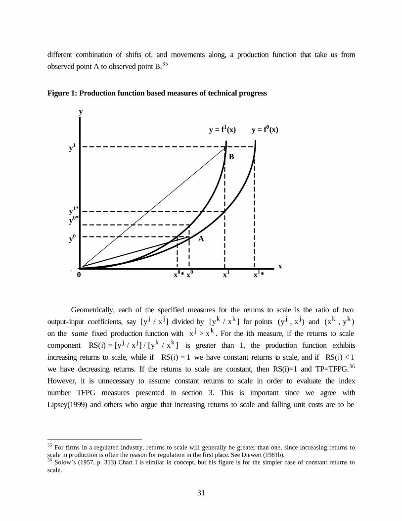
31

different combination of shifts of, and movements along, a production function that take us from observed point A to observed point B.35

Figure 1: Production function based measures of technical progress y y = f1(x) y = f0(x) y1 B y1* y0*

y0 A x 0 x0* x0 x1 x1*

Geometrically, each of the specified measures for the returns to scale is the ratio of two output-input coefficients, say ]x/y[ jj divided by ]x/y[ kk for points )x,y( jj and )y,x( kk on the same fixed production function with kj xx > . For the ith measure, if the returns to scale component ]x/y[/]x/y[)i(RS kkjj= is greater than 1, the production function exhibits increasing returns to scale, while if 1)i(RS = we have constant returns to scale, and if 1)i(RS < we have decreasing returns. If the returns to scale are constant, then RS(i)=1 and TP=TFPG.36 However, it is unnecessary to assume constant returns to scale in order to evaluate the index number TFPG measures presented in section 3. This is important since we agree with Lipsey(1999) and others who argue that increasing returns to scale and falling unit costs are to be

35 For firms in a regulated industry, returns to scale will generally be greater than one, since increasing returns to scale in production is often the reason for regulation in the first place. See Diewert (1981b). 36 Solow’s (1957, p. 313) Chart I is similar in concept, but his figure is for the simpler case of constant returns to scale.

32

expected in many production situations when there are increases in output or when new technologies are introduced.37

6.2 Malmquist Indexes

If the technology for a multiple input, multiple output production process can be represented in each time period by some known production function, this function can be used as a basis for defining theoretical Malmquist quantity and Malmquist TFPG indexes. Malmquist indexes are introduced here, and then in the following subsection we show conditions under which these theoretical Malmquist indexes can be evaluated using the same information needed in order to evaluate the TFPG index numbers introduced in section 3.

Here as previously, we let t1y denote the amount of output 1 produced in period t for

.T,,1,0t K= Here we also let ]y...,,y,y[y~ tM

t3

t2

t ≡ denote the vector of other outputs jointly produced in each period t along with output 1 using the vector of input quantities

]x...,,x,x[x tN

t2

t1

t ≡ . Using these notational conventions, the production functions for output 1 in period s and in period t can be represented compactly as:

(6.2-1) )x,y~(fy ssss1 = and )x,y~(fy tttt

1 = .

Three alternative Malmquist output quantity indexes will be defined. 38 The first Malmquist output index, sα , is the number which satisfies

(6.2-2) )x,/y~(f/y sstsst1 α=α .

This index is the number which just deflates the period t vector of outputs, ]y...,,y,y[y t

Mt2

t1

t ≡ , into an output vector st /y α that can be produced with the period s vector of inputs, sx , using the period s technology. Due to substitution, when the number of output goods, M, is greater than 1, then the hypothetical output quantity vector st /y α will not usually be equal to the actual period s output vector, sy . However, when there is only one output good, then we have s

1ssst

1 y)x(f/y ==α and this first Malmquist output index reduces to s1

t1

s y/y=α . A second Malmquist output index, tα , is defined as the number which satisfies

37 See also Harberger (1998), Basu and Fernald (1997), Nakajima, Nakamura and Yoshioka (1998) and the references provided in those papers. 38 These indexes correspond to the two output indexes defined in Caves, Christensen, and Diewert (1982b, p.1400) and referred to by them as Malmquist indexes because Malmquist (1953) proposed indexes similar to these in concept, though his were for the consumer rather than the producer context. Indexes of this sort were subsequently defined as well by Moorsteen (1961) and Hicks (1961; 1981, pp.192 and 256) for the producer context. See also Balk (1998, ch. 4).

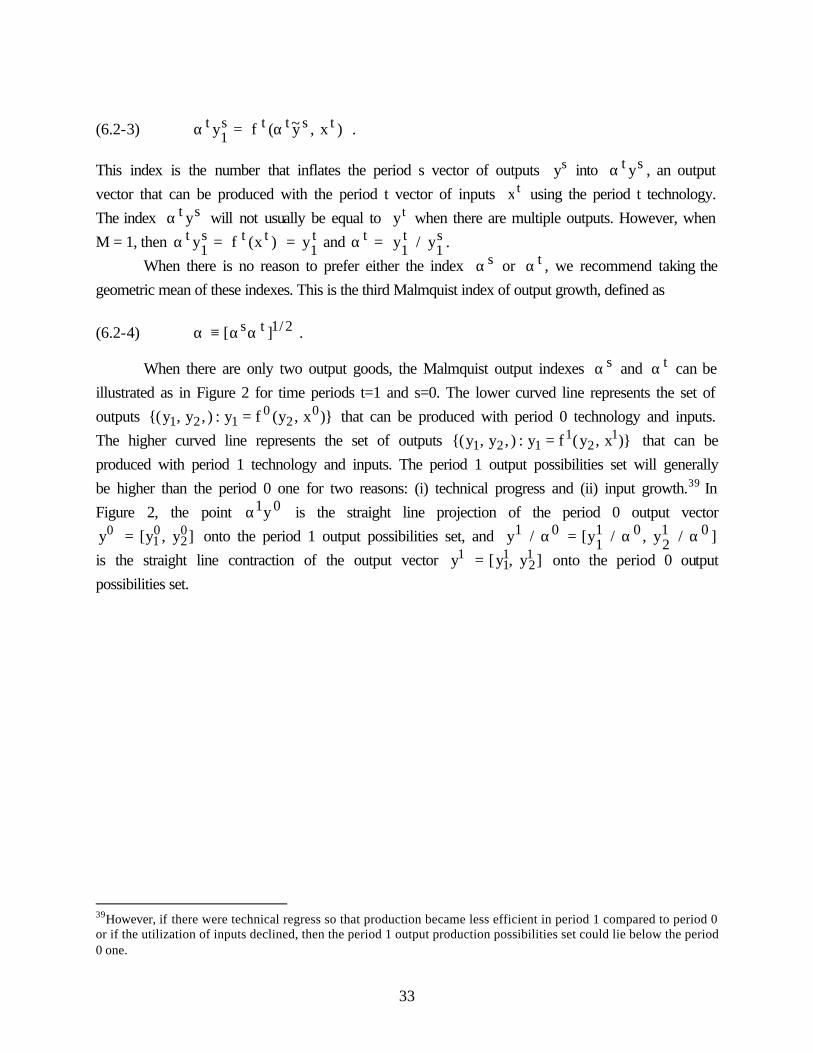
33

(6.2-3) )x,y~(fy tstts1

t α=α .

This index is the number that inflates the period s vector of outputs sy into st yα , an output vector that can be produced with the period t vector of inputs tx using the period t technology. The index st yα will not usually be equal to ty when there are multiple outputs. However, when M = 1, then t

1tts

1t y)x(fy ==α and s

1t1

t y/y=α . When there is no reason to prefer either the index sα or tα , we recommend taking the

geometric mean of these indexes. This is the third Malmquist index of output growth, defined as

(6.2-4) 2/1ts ][ αα≡α .

When there are only two output goods, the Malmquist output indexes sα and tα can be illustrated as in Figure 2 for time periods t=1 and s=0. The lower curved line represents the set of outputs )}x,y(fy:),y,y{( 0

20

121 = that can be produced with period 0 technology and inputs. The higher curved line represents the set of outputs )}x,y(fy:),y,y{( 1

21

121 = that can be produced with period 1 technology and inputs. The period 1 output possibilities set will generally be higher than the period 0 one for two reasons: (i) technical progress and (ii) input growth.39 In Figure 2, the point 01yα is the straight line projection of the period 0 output vector

]y,y[y 02

01

0 = onto the period 1 output possibilities set, and ]/y,/y[/y 012

011

01 αα=α is the straight line contraction of the output vector ]y,y[y 1

211

1 = onto the period 0 output possibilities set.

39However, if there were technical regress so that production became less efficient in period 1 compared to period 0 or if the utilization of inputs declined, then the period 1 output production possibilities set could lie below the period 0 one.

34

Figure 2: Alternative economic output indexes illustrated y2 α 1y2

0 α 1y0

y2

0 y0=(y10,y2

0) y2

1 y1=(y11,y2

1) y2

1/α 0 y1/α 0

y1

(0,0) y10 y1

1/α 0 α 1y10 y1

1

We now turn to the input side. A first Malmquist input index, sβ , is defined as follows:

(6.2-5) )/x...,,/x,y...,,y(f)/x,y~(fy stN

st1

sM

s2

sstsss1 ββ≡β= .

This index measures input growth holding fixed the period s technology and output vector. A second Malmquist input index, denoted by tβ , is the solution to the following equation

(6.2-6) )x...,,x,y...,,y(f)x,y~(fy sN

ts1

ttM

t2

tstttt1 ββ≡β= .

This index measures input growth holding fixed the period t technology and output vector. When there is no reason to prefer sβ to tβ , we recommend a third Malmquist input index:

(6.2-7) 2/1ts ][ ββ≡β .

35

Figure 3 illustrates the Malmquist indexes sβ and tβ for the case where there are just two input goods and for the time periods t=1 and s=0.

Figure 3: Alternative Malmquist input indexes illustrated x2 β 1x2

0 β 1x0

x2

0 x0 = (x10 ,x2

0) x1 = (x1

1,x21)

x21

x2

1/β 0 (0,0) x1

0 β 1x10 x1

1/β 0 x11

The lower curved line in Figure 3 represents the set of inputs that are needed to produce the vector of outputs 0y using period 0 technology. This is the set

)}x,x,y~(fy:)x,x{( 21000

121 = . The higher curved line represents the set of inputs that are needed to produce the period 1 vector of outputs 1y using period 1 technology. This is the set

)}x,x,y~(fy:)x,x{( 21111

121 = .40 The point ]x,x[x 02

101

101 ββ=β is the straight line projection of the input vector ]x ,x[x 0

201

0 ≡ onto the period 1 input requirements set. The point

40 If technical progress were sufficiently positive or if output growth between the two periods were sufficiently negative, then the period 1 input requirements set could lie below the period 0 input requirements set instead of above.

36

]/x,/x[/x 012

011

01 ββ≡β is the straight line contraction of the input vector ]x,x[x 12

11

1 ≡ onto the period 0 input requirements set.

Once theoretical Malmquist quantity indexes have been defined that measure the growth of total output and the growth of total input, then a Malmquist TFPG index for the general N-M case can be defined too. The definition we recommend for the Malmquist TFPG index is (6.2-8) βα≡ /TFPGM .

In the 1-1 case, expression (6.2-8) reduces to TFPG(2) as defined in expression (2.1-3), which

equals the single measure for TFPG for the 1-1 case.

6.3 Direct Evaluation of Malmquist Indexes for the N-M Case

Using the exact index number approach, Caves, Christensen, and Diewert (1982b, pp.1395–1401) give conditions under which the Malmquist output and input quantity indexes

2/1ts ][ αα≡α and 2/1ts ][ ββ≡β defined in (6.2-4) and (6.2-7) equal Törnqvist indexes. More specifically, Caves, Christensen, and Diewert give conditions under which (6.3-1) TQ=α

and

(6.3-2) ,Q*T=β

where TQ is the Törnqvist output quantity index and *TQ is the Törnqvist input quantity index.

The assumptions required to derive (6.3-1) and (6.3-2) are, roughly speaking: (i) price taking, revenue maximizing behavior, (ii) price taking, cost minimizing behavior, and (iii) a translog technology.41 Under these assumptions, we can evaluate the Malmquist measure MTFPG by taking the ratio of the Törnqvist output and input quantity indexes since we have

(6.3-3) T*TTM TFPGQ/Q/TFPG ≡=βα= .

41 An intuitive explanation for the remarkable equalities in (6.3-1) and (6.3-2) rests on the following fact: if f(z) is a

quadratic function, then ]rztz[T)]rz(f)tz(f)[2/1()rz(f)tz(f −∇+∇=− . This result follows from applying Diewert’s (1976, p. 118) Quadratic Approximation Lemma. Under the assumption of optimizing behavior on the

part of the producer, the vectors of first order partial derivatives, )tz(f∇ and )rz(f∇ , will be equal to or proportional to the observed prices. Thus the right-hand side of the above identity becomes observable without estimation. In actual applications of this identity, we assume that various transformations of f are quadratic and apply the resulting identity.

37

The practical importance of (6.3-3) is that the Malmquist TFPG index can be evaluated from observable prices and quantities without knowing the true period specific production functions. Recall that the “best” productivity index from the axiomatic point of view is the Fisher productivity index defined in (3.3-4) as

*FFF Q/QTFPG ≡ ,

with the Fisher output quantity index FQ defined by (3.2-3) and the Fisher input quantity index *FQ defined by (3.2-6). Diewert (1992b, pp.240–243) shows that the Fisher output and input

quantity indexes equal Malmquist indexes under a somewhat different assumption about the nature of the technology from the one required to justify (6.3-1) and (6.3-2). To establish this, the firm’s output distance function over the relevant time span must have the functional form

2/11tT1tt1TTtt ]xByxy)Cxx(Ayy[)x,y(d −−− ⋅β⋅α+σ= . Here T denotes a transpose, the parameter matrices A and C are symmetric and independent of time t, and the parameter vectors

tα and tβ and also the parameter matrix tB can depend on time. The vector 1x − is defined as consisting of components that are the reciprocals of the components of the vector x of input quantities. The parameter matrices and vectors must also satisfy some additional restrictions that are listed in Diewert (1992b, p.241). It should be noted that the above results do not rely on the assumption of constant returns to scale in production. Also, the assumption of revenue maximizing behavior can be dropped if we know the marginal costs in the two periods under consideration, in which case we could directly evaluate the Malmquist indexes. However, usually we do not know these marginal costs. The Fisher is our preferred TFPG index. However, for measuring national productivity, both the Fisher and the Törnqvist indexes should yield similar results.42 Both are superlative index numbers and, as already noted, Diewert (1976, 1978b) and Hill (2000) established that all of the commonly used superlative index number formulas approximate each other to the second order when each index is evaluated at an equal price and quantity point.43 These approximation

42 See Diewert (1978b, p.894). 43 The term superlative means that an index is exact for a flexible functional form. Since the Fisher and the Törnqvist indexes are both superlative, they will both have the same first and second order partial derivatives with respect to all arguments when the derivatives are evaluated at a point where the price and quantity vectors take on the same value for both period t and period s. Peter Hill (1993; p. 384) explains current accepted practice as follows: “Thus economic theory suggests that, in general, a symmetric index that assigns equal weight to the two situations being compared is to be preferred to either the Laspeyres or Paasche indices on their own. The precise choice of superlative index—whether Fisher, Törnqvist or other superlative index—may be of only secondary importance as all the symmetric indices are likely to approximate each other, and the underlying theoretic index fairly closely, at least when the index number spread between the Laspeyres and Paasche is not very great.” Robert Hill (2000) showed that whereas the approximation result of Diewert (1978b) which the remarks of Peter Hill (1993) quoted above are based on and which have found

38

results, and also Diewert’s (1978b) result for the Paasche and Laspeyres indexes, hold without the assumption of optimizing behavior and regardless of whether the assumptions made about the technology are true. These are findings of numerical rather than economic analysis. 7. COST FUNCTION BASED MEASURES

In this section, we define another set of theoretical output and input growth rate and TFPG measures based on the true underlying cost function instead of the production function as in section 6. We give conditions under which these indexes equal the Laspeyres and the Paasche indexes. For the two output case, we also show how the Laspeyres and Paasche indexes relate to the Malmquist indexes defined in the previous section.

Recall from (5-2) that the period t ( T,,1,0t K= ) cost function )w...,,w,w,y...,,y,y(c N21M21

t is the minimum cost of producing the given quantities

M21 y,,y,y K of the M output goods using the input quantities N21 x,,x,x K purchased at the unit prices N21 w,,w,w K and using the period t technology summarized by the production function constraint )x...,,x,x,y...,,y(fy N21M2

t1 = . In this section, we assume that the

period s and period t cost functions, sc and tc , are known and we examine theoretical output, input and productivity indexes that can be defined using these cost functions.

Under the assumptions of perfect information and cost minimizing behavior on the part of the production unit, the actual period t total cost equals the period t cost function evaluated at the period t output quantities and input prices. Thus for the period t cost function, )w,y(c ttt , we have

(7-1) .Cxwxw)w,y(c ttttn

tn

N1n

ttt ≡⋅≡= ∑ =

(As in the above expression, for convenience weighted sums will sometimes be represented as inner products of vectors in addition to, or as an alternative to, the representation of these sums using summation signs.) The cost function in (7-1) is assumed to be differentiable with respect to the components of the vector y at the point )w,y( tt . Under the assumed conditions, the ith marginal cost for period t, denoted by t

imc , is given by

(7-2) itttt

i y/)w,y(cmc ∂∂≡ , i = 1,2,...,M.

their way into the manuals of statistical agencies around the world do indeed apply to all of the commonly used superlative indexes including the Fisher, Törnqvist, and implicit Törnqvist, the approximation can be poor for some

39

Marginal costs for period s are defined analogously. Just as the output unit prices were used as weights for the period s and period t quantities

in the formulas for the Laspeyres and Paasche quantity indexes given in section 3, here the marginal cost vectors, smc and tmc , are used to define theoretical Laspeyres and Paasche type output and input quantity indexes. These indexes are given by

(7-3) sstsL ymc/ymc ⋅⋅≡γ

and

(7-4) stttP ymc/ymc ⋅⋅≡γ .

When we have no reason to prefer Lγ over Pγ , we recommend using as a theoretical measure of the output growth rate the geometric mean of Lγ and Pγ ; that is, we recommend using

(7-5) 2/1PL ][ γγ≡γ .

With price taking, profit maximizing behavior, the observed output quantity vector ty is determined as the solution to the first order necessary conditions for the period t profit maximization problem and economic theory implies that tt mcp = for T,,1,0t K= . If this is the case, then Lγ defined in (7-3) equals the usual Laspeyres output index, LQ , defined in (3.2-2), and Pγ defined in (7-4) equals the usual Paasche output index, PQ , defined in (3.2-1). Moreover, in this case γ defined in (7-5) equals the usual Fisher output index, FQ , defined in (3.2-3).

With just two outputs and under the assumptions of price taking, profit maximizing behavior, the differences between the new theoretical output indexes and LP γγ and the Malmquist output indexes and ts αα can be illustrated using Figure 4.

other superlative indexes.

40

Figure 4: Alternative price based theoretical output indexes y2 α 1y0 y0 y1 y1/α 0 y1 (0,0) A B C D E F

The lower curved line in Figure 4 is the period s=0 output possibilities set, )}x,y(fy :)y ,y{( 0

20

121 = . The higher curved line is the period t=1 output possibilities set, )}x,y(fy:)y,y{( 1

21

121 = . The straight line ending in D is tangent to the period 0 output possibilities set at the observed period 0 output vector ]y ,y[y 0

201

0 ≡ , and the straight line ending in C is tangent to the period 1 output possibilities set at the observed period 1 output vector

]y ,y[y 12

11

1 ≡ . The marginal costs for period 0 and period 1 are denoted by 0imc and 1

imc for outputs i=1,2. The tangent line through 0y , the output quantity vector for period 0, has the slope

)mc/mc( 02

01− and the tangent line through 1y , the period 1 output quantity vector, has the

slope )mc/mc( 12

11− . The straight line ending in E passes through 1y , and the straight line

ending in F passes through 01yα . Both of these lines are parallel to the line ending in D: the tangent to the period 0 output possibility set at the point )y,y( 0

201 . Similarly, the straight line

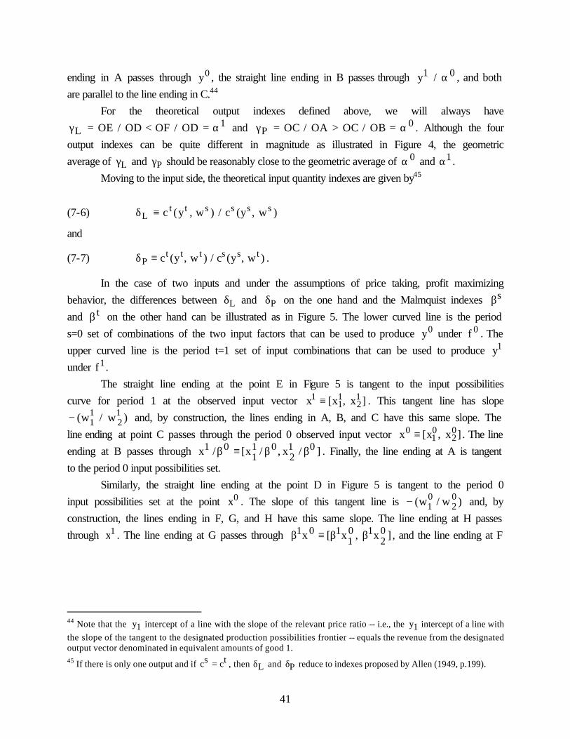
41

ending in A passes through 0y , the straight line ending in B passes through 01 /y α , and both are parallel to the line ending in C.44

For the theoretical output indexes defined above, we will always have 1

L OD/ OFOD/OE α=<=γ and 0P OB/OCOA/OC α=>=γ . Although the four

output indexes can be quite different in magnitude as illustrated in Figure 4, the geometric average of Lγ and Pγ should be reasonably close to the geometric average of 0α and 1α .

Moving to the input side, the theoretical input quantity indexes are given by45

(7-6) )w,y(c/)w,y(c ssssttL ≡δ

and

(7-7) )w,y(c/)w,y(c tsstttP ≡δ .

In the case of two inputs and under the assumptions of price taking, profit maximizing behavior, the differences between Lδ and Pδ on the one hand and the Malmquist indexes sβ and tβ on the other hand can be illustrated as in Figure 5. The lower curved line is the period s=0 set of combinations of the two input factors that can be used to produce 0y under 0f . The upper curved line is the period t=1 set of input combinations that can be used to produce 1y under 1f .

The straight line ending at the point E in Figure 5 is tangent to the input possibilities curve for period 1 at the observed input vector ]x,x[x 1

211

1 ≡ . This tangent line has slope )w/w( 1

211− and, by construction, the lines ending in A, B, and C have this same slope. The

line ending at point C passes through the period 0 observed input vector ]x,x[x 02

01

0 ≡ . The line ending at B passes through ]/x,/x[/x 01

201

101 ββ≡β . Finally, the line ending at A is tangent

to the period 0 input possibilities set. Similarly, the straight line ending at the point D in Figure 5 is tangent to the period 0

input possibilities set at the point 0x . The slope of this tangent line is )w/w( 02

01− and, by

construction, the lines ending in F, G, and H have this same slope. The line ending at H passes through 1x . The line ending at G passes through ]x ,x[x 0

210

1101 ββ≡β , and the line ending at F

44 Note that the 1y intercept of a line with the slope of the relevant price ratio -- i.e., the 1y intercept of a line with the slope of the tangent to the designated production possibilities frontier -- equals the revenue from the designated output vector denominated in equivalent amounts of good 1. 45 If there is only one output and if tcsc = , then Lδ and Pδ reduce to indexes proposed by Allen (1949, p.199).

42

is tangent to the period 1 input possibilities curve. It can be shown that 1

L OD/OGOD/OF β=<=δ and 0P OB/OEOA/OE β=>=δ .46

Figure 5: Alternative price based economic input indexes x2 x1 β 1x0 x1/β 0 x0 (0,0) A B C E D F G H

46 The tangency relation follows using Shephard’s (1953, p.11) Lemma: 1w/)0

2w,01w,0y(0c0

1x ∂∂= and

2w/)02w,0

1w,0y(0c02x ∂∂= . Similarly, the fact that the tangent line ending at E has slope equal to 1

2w/11w

follows from 1w/)12w,1

1w,1y(1c11x ∂∂= and 2w/)1

2w,11w,1y(1c1

2x ∂∂= . Note that the 1x intercept of a line

with the slope of )02w/0

1w(− , as is the case for the lines ending in D, F, G or H, or of a line with the slope of

)12w/1

1w(− , as is the case for the lines ending in A, B, C or D, is equal to the cost of the stated input vector

denominated in units of input factor 1.

43

8. THE DIEWERT-MORRISON PRODUCTIVITY MEASURE AND DECOMPOSITIONS

In section 5, we used the period t production function tf to define the period t cost function, tc . The period t production function can also be used to define the period t (net) revenue function: (8-1)

T,,1,0t )};x;y,,y(fy);y,,y,y(y:yp{max)x,p(r M2t

1M21yt KKK ==≡⋅≡

where )p,,p(p M1 K≡ is the output price vector that the producer faces and )x,,x(x N1 L≡ is the input vector.47 Diewert and Morrison (1986) use revenue functions for period t and the comparison period s to define another family of theoretical productivity growth indexes:

(8-2) )x,p(r/)x,p(r)x,p(RG st≡ .

This index is the ratio of the net value of the output that can be produced using the period t versus the period s technology but holding the inputs constant at the quantities given in some reference net input quantity vector x and the prices constant at some reference unit price vector, p. This is a different approach to the problem of controlling for total factor input utilization in judging the success of the period t versus the period s production outcomes. Two special cases of (8-2) are of interest: (8-3)

)x,p(r/)x,p(r)x,p(RGRG and )x,p(r/)x,p(r)x,p(RGRG ttsttttttssssstsss =≡=≡ .

The first of these, sRG , is the theoretical productivity index obtained by letting the reference vectors p and x take on the observed period s values. The second of these, tRG , is the theoretical productivity index obtained by letting the reference vectors be the observed period t output price vector tp and input quantity vector tx .48

Under the assumption of revenue maximizing behavior in both periods, we have:

47 If ym is positive (negative), then the net output m is an output (input). We assume that all output prices pm are positive. We assume that all input quantities xn are positive and if the net input n is an input (output), then wn is positive (negative). 48 This approach can be viewed as an extension to the general N-M case of the methodology used in defining the output based measures of technical progress given in (6.1-7) and (6.1-8).

44

(8-4) )x,p(ryp and )x,p(ryp sssssttttt =⋅=⋅

If these equalities hold, this means we observe values for the denominator of sRG and the numerator of tRG . However, we cannot directly observe the terms, )x,p(r sst and )x,p(r tts . The first of these is the hypothetical revenue that would result from using the period t technology with the period s input quantities and output prices. The second is the hypothetical revenue that would result from using the period s technology with the period t input quantities and output prices. These hypothetical revenue figures can be inferred from observable data if we know the functional form for the period t revenue function and it is associated with an index number formula that can be evaluated with the observable data. Suppose, for example, that the revenue function has the following translog functional form:

(8-5) nm

M1m

N1n mnjn

N1n

N1j nj

jmM

1mM

1j mjnN

1ntnm

M1m

tm

ts

t

nxnpnxnx)2/1(

npnp)2/1(nxnp)x,p(nr

llll

lllll

∑ ∑∑ ∑

∑ ∑∑∑

= == =

= ===

γ+β+

α+β+α+α≡

where jmmj α=α and jnnj β=β and the parameters satisfy various other restrictions to ensure that r t(p,x) is linearly homogeneous in the components of the price vector p.49 Note that the coefficient vectors t

ntm

t0 and , βαα can be different in each time period but that the quadratic

coefficients are assumed to be constant over time. Diewert and Morrison (1986; p. 663) show that under the above assumptions, the

geometric mean of the two theoretical productivity indexes defined in (8-3) can be identified using the observable price and quantity data that pertain to the two periods; i.e., we have

(8-6) bc/a]RGRG[ 2/1ts =

where a, b and c are given by

(8-7) sstt yp/ypa ⋅⋅≡ ,

(8-8) )p/p(n)]yp/yp()yp/yp)[(2/1(nb sm

tm

tttm

tm

sssm

M1m

sm ll ⋅+⋅≡ ∑ = , and

(8-9) )x/x(n)]yp/xw()yp/xw)[(2/1(nc sn

tn

tttn

tn

sssn

N1n

sn ll ⋅+⋅= ∑ = .

If we have constant returns to scale production functions sf and tf , then the value of outputs will equal the value of inputs in each period and we have

49 These conditions can be found in Diewert (1974a, p. 139). The derivation of (6.3-1) and (6.3-2) also required the assumption of a translog technology.

45

(8-10) tttt xwyp ⋅=⋅ .

The same result can be derived without the constant returns to scale assumption if we have a fixed factor that absorbs any pure profits or losses, with this fixed factor defined as in (5-18) in section 5.

Substituting (8-10) into (8-9), we see that expression c becomes the Törnqvist input index *TQ . By comparing (8-8) and (3.8-2), we see also that b is the Törnqvist output price index TP .

Thus b/a is an implicit Törnqvist output quantity index. If (8-10) holds, then we have the following decomposition for the geometric mean of the

product of the theoretical productivity growth indexes defined in (8-3):

(8-11) ]QP/[]yp/yp[]RGRG[ *TT

sstt2/1ts ⋅⋅= ,

where TP is the Törnqvist output price index defined in (3.8-2) and *TQ is the Törnqvist output

quantity index defined analogously to the way in which the Törnqvist output quantity index is defined in (3.8-1). Diewert and Morrison (1986) use the period t revenue functions to define two theoretical output price effects which show how revenues would change in response to a change in a single output price:

(8-12) M,1,m ),x,p(r/)x,p,,p,p,p,,p(rP sssssM

s1m

tm

s1m

s1

ssm KKK =≡ +− ,

and

(8-13) M,1,m ),x,p,,p,p,p,,p(r/)x,p(rP ttM

t1m

sm

t1m

t1

tttttm KKK =≡ +− .

More specifically, these theoretical indexes give the proportional changes in the value of output that would result if we changed the price of the mth output from its period s level s

mp to its period t level t

mp holding constant all other output prices and the input quantities at reference levels and using the same technology in both situations. For the theoretical index defined in (8-12), the reference output prices and input quantities and technology are the period s ones, whereas for the index defined in (8-13) they are the period t ones. Now define the theoretical output price effect mb as the geometric mean of the two effects defined by (8-12) and (8-13):

(8-14) M,,1m ,]PP[b 2/1tm

smm K=≡ .

Diewert and Morrison (1986) and Kohli (1990) show that the bm given by (8-14) can be evaluated by the following observable expression, provided that conditions (8-4), (8-5) and (8-10) hold:

46

(8-15) M,1,m ),p/p(n)]yp/yp()yp/yp)[(2/1(nb sm

tm

tttm

tm

sssm

smm Kll =⋅+⋅= .

Comparing (8-8) with (8-15), it can be seen that we have the following decomposition for b:

(8-16) TmM

1m Pbb =∏= = .

Thus the overall Törnqvist output price index, TP , can be decomposed into a product of the individual output price effects, mb .

Diewert and Morrison (1986) also use the period t revenue functions in order to define two theoretical input quantity effects as follows:

(8-17) N,1,n ),x,p(r/)x,,x,x,x,,x,p(rQ ssssN

s1n

tn

s1n

s1

sss*n KKK =≡ +−

and

(8-18) N.,1,n ),x,,x,x,x,,x,p(r/)x,p(rQ tN

t1n

sn

t1n

t1

tttttt*n KKK =≡ +−

These theoretical indexes give the proportional change in the value of output that would result from changing input n from its period s level s

nx to its period t level tnx , holding constant all

output prices and other input quantities at reference levels and using the same technology in both situations. For the theoretical index defined by (8-17), the reference output prices and input quantities and the technology are the period s ones, whereas for the index given in (8-18) they are the period t ones.

Now define the theoretical input quantity effect nc as the geometric mean of the two effects defined by (8-17) and (8-18):

(8-19) N,1,n ,]QQ[c 2/1t*n

s*nn K=≡ .

Diewert and Morrison (1986) show that the nc defined by (8-19) can be evaluated by the following empirically observable expression provided that assumptions (8-4) and (8-5) hold:

(8-20) )x/x(n)]yp/xw()yp/xw)[(2/1(nc sn

tn

tttn

tn

sssn

snn ll ⋅+⋅=

(8-21) )x/x(n)]xw/xw()xw/xw)[(2/1( sn

tn

tttn

tn

sssn

sn l⋅+⋅= .

The expression (8-21) follows from (8-20) provided that the assumptions (8-10) also hold. Comparing (8-20) with (8-9), it can be seen that we have the following decomposition for c:

(8-22) ∏ == N1n ncc

47

(8-23) *TQ = ,

where (8-23) follows from (8-22) provided that the assumptions (8-10) also hold. Thus if assumptions (8-4), (8-5) and (8-10) hold, the overall Törnqvist input quantity index can be decomposed into a product of the individual input quantity effects, the nc for

.N,,1n K= . Having derived (8-16) and (8-22), we can substitute these decompositions into (8-6) and rearrange the terms to obtain the following very useful decomposition:

(8-24) ∏∏ ===⋅⋅ N1n n

M1m m

2/1tssstt cb]RGRG[yp/yp

This is a decomposition of the growth in the nominal value of output into the productivity growth term 2/1ts ]RGRG[ times the product of the output price growth effects, the mb , times the product of the input quantity growth effects, the nc . All of the effects on the right-hand side of expression (8-24) can be calculated using only the observable price and quantity data pertaining to the two periods.50 An interesting special case of (8-24) results when there is only one input in the x vector and it is fixed. Then the input growth effect 1c is unity and variable inputs appear in the y vector with negative components. In this special case, the left-hand side of (8-24) becomes the pure profits ratio that is decomposed into a productivity effect times the various price effects (the

mb ).

9. THE DIVISIA APPROACH

In the discrete time approaches to productivity measurement, the price and quantity data are defined only for integer values of t where each value that the index t takes on denotes a particular discrete unit time period. Indexes have been defined for this discrete time data that reflect change from some comparison period s to some current period t. In contrast, in Divisia’s (1926; 40) approach to the measurement of aggregate input and output, the data are regarded as continuous time variables.51 To emphasize the continuous time feature of the Divisia approach, in this section the price and quantity of output m at time t are denoted by )t(pm and )t(ym for goods M,,2,1m K= and the price and quantity of input n at time t are denoted by )t(wn and 50 See Morrison and Diewert (1990) for decompositions for other functional forms besides the translog. Kohli (1990) and Fox and Kohli (1998) use (8-24) to examine the factors behind the growth in the nominal GDP of several countries. 51 See Hulten (1973). For a comprehensive review of the Divisia approach, see also Balk (2000).

48

)t(xn for factors N,,2,1N K= . It is assumed that these price and quantity functions are differentiable with respect to time over the interval 1t0 ≤≤ . Revenue and cost can be represented as (9-1) )t(y)t(p)t(R mm

M1m∑ =≡

and

(9-2) )t(x)t(w)t(C nnN

1n∑ =≡ .

Differentiating both sides of (9-1) with respect to time and dividing by R(t), we obtain (9-3)

)]t(R/)t(y)t(p[)]t(y/)t(y[

)]t(R/)t(y)t(p[)]t(p/)t(p[[

)t(R/)]t(y)t(p)t(y)t(p[)t(R/)t('R

mmm'm

M1m

mmm'm

M1m

'mm

M1mm

'm

M1m

∑

∑

∑∑

=

=

==

+

=

+=

(9-4) )t(s)]t(y/)t(y[)t(s)]t(p/)t(p[ Rmm

'm

M1m

Rmm

'm

M1m ∑∑ == += ,

where a prime denotes the time derivative of a function and )t(R/)]t(y)t(p[)t(s mmRm ≡ is the

revenue share of output m at time t for m = 1, 2, ..., M. The left-hand side of (9-4) is )t(R/)t('R which is the (percentage) rate of change in revenue at time t. The first set of terms on the right-hand side of (9-4) is a revenue share weighted sum of the rates of growth in the prices. Divisia (1926, p.40) simply defined this sum to be the percentage rate of change of an aggregate output price at time t, P(t).52 That is, Divisia defined the aggregate price growth rate to be

(9-5) )t(s)]t(p/)t(p[)t(P/)t('P Rmm

'm

M1m∑ =≡ .

The second set of terms on the right-hand side of (9-4) is a revenue share weighted sum of the rates of growth for the output quantities of the individual output goods. Divisia defined these terms to be the percentage rate of change of an aggregate quantity at time t, Y(t). That is, Divisia defined the aggregate output quantity growth rate to be

(9-6) ∑≡ )t(s )]t(y/)t(y[)t(Y/)t('Y Rmm

'm .

Substituting (9-5) and (9-6) into (9-4) yields:

52 This is much like declaring the Törnqvist output index to be a measure of output price growth, since it is a weighted aggregate of the growth rates for the prices of the individual output goods.

49

(9-7) )t(Y/)t('Y)t(P/)t('P)t(R/)t('R += .

In words, (9-7) says that revenue growth at time t is equal to aggregate output price growth plus aggregate output quantity growth at time t. Equation (9-7) is the Divisia index counterpart to the output side product test decomposition. A decomposition similar to (9-7) can be derived in the same way for the (percentage) rate of growth in cost at time t, )t(C/)t('C . Differentiating both sides of (9-2) with respect to t and dividing both sides by )t(C yields

(9-8) ).t(s )]t(x/)t(x[)t(s )]t(w/)t(w[

)t(C/)]t('x)t(w)t(x)t('w[)t(C/)t('C

Cnn

'n

N1n

Cnn

'n

N1n

nnN

1nnnN

1n

∑∑

∑∑

==

==

+=

+=

Here )t(w'n is the rate of change of the nth input price, )t(x '

n is the rate of change of the nth input quantity, and )t(C/)]t(x)t(w[)t(s nn

Cn ≡ is the input n share of total cost at time t.

Let W(t) and X(t) denote the Divisia input price and input quantity aggregates evaluated at time t, where their proportional rates of change are defined by the two cost share weighted sums of the rates of growth of the individual microeconomic input prices and quantities:

(9-9) )t(s )]t(w/)t(w[)t(W/)t('W Cnn

'n

N1n∑ =≡

and

(9-10) )t(s )]t(x/)t(x[)t(X/)t('X Cnn

'n

N1n∑ =≡ .

Substituting (9-9) and (9-10) into (9-8) yields the following input side version of equation

(9-7):

(9-11) )t(X/)t('X)t(W/)t('W)t(C/)t('C += .

In words, (9-11) says that the rate of growth in cost is equal to aggregate input price growth plus aggregate input quantity growth at time t. Equation (9-11) is the Divisia index counterpart to the input side product test decomposition in the axiomatic approach to index number theory. Jorgenson and Griliches (1967, p.252) define the Divisia TFPG index at time t as the rate of growth of the Divisia output index minus the rate of growth of the Divisia input index,53 (9-12) )]t(X/)t('X[)]t(Y/)t('Y[)t(TFPG −≡ ,

53 Note that the Divisia productivity measure is defined as a difference in rates of growth whereas our previous productivity definitions all involved taking a ratio of growth rates. However, the log of a ratio equals the difference of the logs, so this distinction is not necessarily important.

50

where )t(Y/)t('Y is given by (9-6) and )t(X/)t('X is given by (9-10). For the one output, one input case when t = 0, we let )t(y)t(y)t(Y 1 == and

)t(x)t(x)t(X 1 == . In order to operationalize the continuous time approach, we approximate the derivatives with finite differences as follows:

(9-13) 01 yy)0(y)1(y)0('y)0('Y −=−≅=

and

(9-14) 01 xx)0(x)1(x)0('x)0('X −=−≅= .

Substituting these approximations into (9-12) yields (9-15) )]0(x/)0('x[)]0(y/)0('y[)0(TFPG −= ,

which is the Divisia approach counterpart to (2.1-3). Returning to the general Divisia productivity measure defined by (9-12), Jorgenson and Griliches (1967, p.252) develop an analogous result for the general N input, M output case under the additional assumption that costs equal revenue at each point in time. In this case we have

)t(C/)t('C)t(R/)t('R = and hence the right-hand sides of (9-7) and (9-11) can be equated. Rearranging the resulting equation and applying (9-12) yields: (9-17) )t(TFPG)]t(X/)t('X[)]t(Y/)t('Y[)]t(P/)t('P[)]t(W/)t('W[ ≡−=− .

Thus, under assumption (9-16), the Divisia TFPG measure equals the Divisia input price growth rate minus the Divisia output price growth rate. The Divisia productivity index defined by (9-12) was related to measures of production function shift by Solow (1957) in the case of one output and two inputs, and by Jorgenson and Griliches (1967) in the N input, M output case. Solow and also Jorgenson and Griliches adopted this framework in their early growth accounting studies, as we shall discuss in section 10. These authors assumed constant returns to scale, so their analysis cannot be applied directly to situations where this assumption is inappropriate. However, Denny, Fuss and Waverman (1981, pp.196–199) relate the Divisia TFP measure defined by (9-12) to shifts in the cost function without assuming constant returns to scale. Here we summarize the analysis of Denny, Fuss and Waverman using slightly different notation than they did. Up to this point, our discussion of the Divisia indexes has made no mention of cost minimizing behavior. The approach of Denny, Fuss and Waverman requires us to assume that the productive unit continuously minimizes costs for 1t0 ≤≤ . The production unit’s cost function is )t,w,y(c where )]t(y...,),t(y[)t(y M1≡ denotes the vector of outputs and

)]t(w...,),t(w[)t(w N1≡ denotes the vector of input prices. (The t variable in )t,w,y(c is

51

viewed as representing the fact that the cost function is continuously changing due to technical progress over time.) Under the assumption of cost minimizing behavior for 1t0 ≤≤ , we have54

(9-18) ]t),t(w),t(y[c)t(x)t(w)t(C nnN

1n =≡ ∑ = .

We define the continuous time technical progress measure as minus the (percentage) rate of increase in cost at time t: (9-19) ]t),t(w),t(y[c/}t/]t),t(w),t(y[c{)t(TP ∂∂−≡ .

Shephard’s (1953, p.11) Lemma implies that the partial derivative of the cost function with respect to the nth input price equals the cost minimizing demand for input n, given by: (9-20) nn w/]t),t(w),t(y[c)t(x ∂∂= , n = 1, 2..., N.

Differentiating both sides of (9-18) with respect to t, dividing both sides of the resulting equation by C(t), and using (9-19) and (9-20), we obtain (9-21) )]t(C/)t('y[}y/]t),t(w),t(y[c{)t(C/)t('C mm

M1m ∂∂≡ ∑ =

)t(TP)]t(C/)t('w[)t(x nnN

1n −+ ∑ =

),t(TP)]t(w/)t('w[)t(s)]t(y/)t('y[)t( nnCn

N1nmmm

M1m −+ε= ∑∑ ==

where )}t(y/]t),t(w),t(y[c{/}y/]t),t(w),t(y[c{)t( mmm ∂∂≡ε is the elasticity of cost with respect to the mth output quantity and )t(C/)]t(x)t(w[)t(s nn

Cn ≡ is the nth input cost share.

Denny, Fuss, and Waverman (1981, p.196) define the rate of change of the continuous time output aggregate, Q(t), as follows: (9-22) )t(/)]t(y/)t('y[)t()t(Q/)t('Q i

M1immm

M1m εε≡ ∑∑ == .

Recall that the Divisia expression for the output growth rate given in (9-6) weights the individual output growth rates, )t(y/)t('y mm , by the revenue shares, )t(sR

m . Alternatively, in (9-22), )t(y/)t('y mm is weighted by the mth cost elasticity share, )t(/)t( i

M1im εε ∑ = . It can be shown

54To reconcile the notation used here with the notation used in previous sections, note that

]0),0(w),0(y[c)0w,0y(0c = and ]1),1(w),1(y[c)1w,1y(1c = with ty)t(y ≡ and tw)t(w ≡ for t = 0, 1.

52

that )t(iM

1i ε∑ = is the percentage increase in cost due to a one percent increase in scale for each output.55 We define the reciprocal of this sum to be a measure of (local) returns to scale:

(9-23) 1i

M1i )]t([)t(RS −

= ε≡ ∑ .

Now equate the right-hand side of (9-11) to the right-hand side of (9-21). Using (9-9), (9-22), and (9-23), we obtain the following decomposition of the technical progress measure in terms of returns to scale, output growth and input growth:

(9-24) )]t(X/)t('X[)]t(Q/)t('Q[)]t(RS[)t(TP 1 −= − .

In order to relate the technical progress measure TP(t) defined by (9-19) to the Divisia productivity measure TFPG(t) defined by (9-12), we use equation (9-12) to solve for

)t(TFPG]t(Y/)t('Y[)t(X/)t('X −= and use equation (9-25) to solve for )t(X/)t('X . Equating these two expressions for )t(X/)t('X and rearranging terms yields

(9-25) )t(TP)]t(Q/)t('Q[)]t(RS[)]t(Y/)t('Y[)t(TFPG 1 +−= −

(9-26) )]}t(Q/)t('Q[)]t(Y/)t('Y[{})]t(RS[1{)}t(Q/)t('Q{)t(TP 1 −+−+= − .

Equation (9-25) is due to Denny, Fuss, and Waverman (1981, p.197). This equation says that the Divisia productivity index equals the technical progress measure TP(t) plus the marginal cost weighted output growth index, )t(Q/)t('Q , times a term that depends on the returns to scale term, { 1)]t(RS[1 −− }, that will be positive if and only if the local returns to scale measure )t(RS is greater than 1, plus the difference between the Divisia output growth index, )t(Y/)t('Y , and the marginal cost weighted output growth index, )t(Q/)t('Q . Denny, Fuss, and Waverman (1981, p.197) interpret the term )t(Q/)t('Q)t(Y/)t('Y − as the effect on TFPG of nonmarginal cost pricing of a nonproportional variety. Their argument goes like this. Suppose that the mth marginal cost is proportional to the period t selling price

)t(pm for m = 1, 2, ..., M. Let the common factor of proportionality be )t(λ Then we have: (9-27) )t(p)t(y/]t),t(w),t(y[c mm λ=∂∂ m = 1, 2, ..., M.

55 The elasticity of cost with respect to a scale variable k is defined as ]}t),t(w),t(y[c/1{ times the following derivative evaluated at k = 1:

)t(mM

1m]t),t(w),t(y[cmy/)t),t(w),t(y(c)t(myM1mk/]t),t(w),t(ky[c ε∑ ==∂∂∑ ==∂∂

where the last equality follows from the definition of )t(mε below (9-21). Therefore, the elasticity of cost with

respect to scale equals )t(mM

1m)t(mM

1m]}y),t(w),t(y[c{]}t),t(w),t(y[c/1{ ε∑ ==ε∑ = .

53

Using (9-27) together with the definitions of )t(mε and )t(sRm , we find that

(9-28) )t(C/)t(R)t()t(s)t( Rmm λ=ε m = 1,2,...,M.

Substituting (9-28) into (9-21) and using (9-6) yields (9-29) )t(Q/)t('Q)t(Y/)t('Y = .

Hence, if marginal costs are proportional to output prices56 (i.e., if (9-27) holds), then the term )t(Q/)t('Q)t(Y/)t('Y − vanishes from (9-26). Note also that if there is only one output good,

then (9-28) and (9-29) will automatically hold. In this case, (9-26) can be rewritten as follows: (9-30) )]t(Y/)t('Y[))]t(RS/1(1[)t(TP)t(TFPG −+= .

Equation (9-30) is analogous to equation (6.1-11) where, for the one input, one output case, we decomposed TFPG into the product of a technical progress term and a returns to scale term. In both of these equations, if output growth is positive and returns to scale are greater than one, then productivity will exceed technical progress. Since the continuous time approach to productivity measurement due to Divisia (1926) and Jorgenson and Griliches (1967) is justified without the assumption of optimizing behavior on the part of the producer, it provides a continuous time counterpart to the discrete time product test decomposition. However, in that approach, constant returns to scale and marginal cost pricing were assumed. On the other hand, the continuous time approach to productivity measurement due to Denny, Fuss and Waverman (1981) relies on the assumption of optimizing behavior, but without the assumption of constant returns to scale and allowing for nonmarginal cost pricing. This second approach provides a continuous time counterpart to the economic approaches to productivity measurement developed in previous sections. We conclude this section with brief comments on the problems associated with the continuous time approaches discussed in this section. First, as already noted, in order to make operational any continuous time approach to productivity measurement, it is necessary to replace derivatives such as )t(y '

m by finite differences such as ( )ty)1t(y mm −+ or ( )1ty)t(y mm −− . The apparent precision of the Divisia approach vanishes when we consider these discrete data approximation problems.

56 It can be shown that if the firm (i) maximizes revenues holding constant its utilization of inputs and (ii) minimizes costs holding constant its production of outputs, then marginal costs will be proportional to output prices; i.e., we

obtain tytmc/tmctytp/tp ⋅=⋅ . Hence prices in period t, tp , are proportional to marginal costs, tmc . It should be noted that assumptions (i) and (ii) above are weaker than the assumption of overall profit maximizing behavior.

54

Diewert (1980, pp.444–446) shows that there are a wide variety of discrete time approximations to the continuous time Divisia indexes. More recently, Balk (2000) shows how virtually all major bilateral index number formulas can be derived using various discrete approximations to the Divisia continuous time index. Second, as we make the period of time shorter and shorter, price and quantity data for purchases and sales become “lumpy” and it is necessary to smooth out these lumps. There is no unique way of doing this smoothing. Third, producers do not optimize at each instant of time. In addition, price and more importantly, quantity data are not available on a continuous time basis. 10. GROWTH ACCOUNTING Growth accounting provides a residual measure of TFPG. Despite the differences in terms and presentation between the growth accounting and index number literatures, the growth accounting measure of productivity growth is, in fact, an index number. The form of the growth accounting TFPG index depends on the functional form of the production function used in specifying the growth accounting framework.57 Because the growth accounting measure of TFPG is an index number, all of the material in earlier sections of this chapter is relevant to growth accounting as well. Hence, our treatment of this approach is limited to illustrating how the growth accounting framework is constructed, noting where important assumptions enter, and outlining issues concerning the measurement of the quantity and price variables that enter into a growth accounting study and the meaning of the resulting TFPG measure: issues that are relevant to the empirical implementation of all measures of national TFPG.

57 The correspondences that can be worked out between the particular functional forms for the selected production function and the resulting growth accounting TFPG measure are part of the exact approach to index numbers, outlined in section 5.

55

10.1 Solow’s 1957 Paper58

Solow’s classic 1957 paper, “Technical Change and the Aggregate Production Function,” provides a convenient context for introducing the basics of growth accounting. This study also influenced many of the subsequent growth accounting studies. As in most studies of this sort, Solow begins with a production function: (10.1-1) )t;L,K(FY = .

Y denotes an output quantity aggregate, K and L are aggregate measures for the capital and labor inputs, and t denotes time.59 Solow states that the variable t “for time” appears in the production function F “to allow for technical change.” However, having introduced t in this way, he goes on to observe that this operational definition in no way singles out the adoption of new production technologies. Indeed, he notes that “slowdowns, speed-ups, improvements in the education of the labor force, and all sorts of things will appear as ‘technical change.’” In specifying the true production function, Solow assumes that technical change can be represented as shifts in the underlying true production function that leave all marginal rates of substitution unchanged and that are associated with the passage of time but not with expenditures on physical capital or labor. Under these assumptions, the production function in (10.1-1) can be rewritten as (10.1-2) )L,K(f)t(AY ⋅= .

That is, under the stated assumptions the production function can be decomposed into a time varying multiplicative technical change term and an atemporal production function.60 The multiplicative factor, A(t), in (10.1-2) represents the effects of shifts over time after controlling for the growth of K and L. Solow re-formulates the output and capital input variables as (Y/L)=y and (K/L)=k. He assumes that the production function is homogeneous of degree one (constant returns to scale), and that capital and labor are paid their marginal products so that total revenue equals the sum of all factor costs. Making use of these assumptions and the Divisia methodology, Solow arrives at the following growth accounting equation: 58 Portions of this section draw on Diewert (1993a, section 3; 1992b, section 5; 1981a, section 7; and 1978b). 59 A host of index number and aggregation issues are subsumed in the construction of the Y, K and L data series. 60 Solow’s recommendations in his 1957 paper encouraged other researchers to be interested in measuring efficiency improvement in their econometric studies by the ratio of period t and period s efficiency parameters, as in (5-5), with the production function for each period specified as the product of a time varying efficiency parameter and an atemporal production function f, as in (5-4).

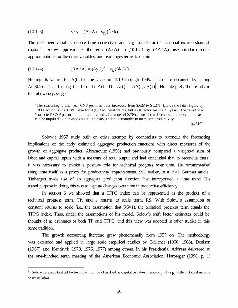
56

(10.1-3) )k/k(s)A/A(y/y K&&& += .

The dots over variables denote time derivatives and Ks stands for the national income share of capital.61 Solow approximates the term )A/A( & in (10.1-3) by )A/A(∆ , uses similar discrete approximations for the other variables, and rearranges terms to obtain (10.1-4) )k/k(s)y/y()A/A( k ∆−∆=∆ .

He reports values for A(t) for the years of 1910 through 1949. These are obtained by setting A(1909) =1 and using the formula [ ])t(A/)t(A1)t(A)1t(A ∆+=+ . He interprets the results in the following passage:

“The reasoning is this: real GNP per man hour increased from $.623 to $1.275. Divide the latter figure by 1.809, which is the 1949 value for A(t), and therefore the full shift factor for the 40 years. The result is a ‘corrected’ GNP per man hour, net of technical change, of $.705. Thus about 8 cents of the 65 cent increase can be imputed to increased capital intensity, and the remainder to increased productivity”

(p. 316). Solow’s 1957 study built on other attempts by economists to reconcile the forecasting implications of the early estimated aggregate production functions with direct measures of the growth of aggregate product. Abramovitz (1956) had previously compared a weighted sum of labor and capital inputs with a measure of total output and had concluded that to reconcile these, it was necessary to invoke a positive role for technical progress over time. He recommended using time itself as a proxy for productivity improvements. Still earlier, in a 1942 German article, Tinbergen made use of an aggregate production function that incorporated a time trend. His stated purpose in doing this was to capture changes over time in productive efficiency. In section 6 we showed that a TFPG index can be represented as the product of a technical progress term, TP, and a returns to scale term, RS. With Solow’s assumption of constant returns to scale (i.e., the assumption that RS=1), the technical progress term equals the TFPG index. Thus, under the assumptions of his model, Solow’s shift factor estimates could be thought of as estimates of both TP and TFPG, and this view was adopted in other studies in this same tradition. The growth accounting literature grew phenomenally from 1957 on. The methodology was extended and applied in large scale empirical studies by Griliches (1960, 1963), Denison (1967) and Kendrick (1973, 1976, 1977) among others. In his Presidential Address delivered at the one-hundred tenth meeting of the American Economic Association, Harberger (1998, p. 1)

61 Solow assumes that all factor inputs can be classified as capital or labor; hence Ks1Ls −= is the national income share of labor.

57

describes growth accounting as an important success story for the economics profession, and asserts that the work of Jorgenson and Griliches (1967), Jorgenson, Gollop and Fraumeni (1987), and Jorgenson (1995a, 1995b) has carried growth accounting to the level of a “high art.” Aspects of the research of Jorgenson and his associates relating to measurement are the subject matter of the remainder of this section.

10.2 Input Factor Measurement and Jorgenson’s Contributions

Researchers such as Jorgenson have struggled to improve our understanding of the workings of the aggregate economy by improving the measurement of the capital and labor quantity and price variables, and also our understanding of the returns in enhanced output resulting from different sorts of input growth. Of course, by better explaining the portions of output growth that are due to increased use of specific sorts of factor inputs, measured TFPG will typically be reduced. This is so for all of the TFPG index number formulas that have been presented. Thus we have the paradoxical result that progress in measuring TFPG can manifest itself in the form of falling values of TFPG over time. We first take up issues in the measurement of the labor input, and then turn to related capital measurement issues. 10.2.1 Measuring the labor input Jorgenson (1995a) observes that Solow’s (1957) definition of investment is limited to tangible assets and argues that this narrow definition is one reason why Solow attributed so much of U.S. economic growth to “residual” growth in productivity. According to Jorgenson, in computing the labor aggregate, hours of work of persons with differing stocks of human capital should be weighted by their differing marginal products. In a 1967 paper, Jorgenson and Griliches present a constant quality index for labor with workers differentiated by their educational attainment.62 More recently, Gollop and Jorgenson (1980, 1983) produced constant quality indexes of labor input for 51 industrial sectors of the U.S. economy. They disaggregated the labor input for each industry by age, sex, educational attainment, class of employment, and occupation.63 As part of this research effort, they created

62 In implementing this approach, he built on earlier research by Griliches and Denison. So-called constant quality indexes of labor input were developed by Griliches (1960) for U.S. agriculture and by Denison (1962) for the U.S. economy as a whole. 63 It is important to note that age and sex are not productive attributes. These are proxy variables, totally immutable by individual effort, that have relationships to productive attributes; moreover, these relationships have been systematically shifting over time. One argument for the use of these particular proxies is that they give rise to more stable results than other categorizations that might be used. However, it is also important to guard against introducing systemic but largely invisible statistical discrimination through the way in which statistical evidence

58

an extensive data base of hours worked and hourly compensation for the specified categories of labor input.64 These so-called constant quality labor input indexes are straightforward applications of index number theory to the measurement of the quantity of labor, though the inclusion in the labor aggregate of certain segments of the out of work potential labor force is controversial and forces consideration of the objectives of TFPG measurement. For example, Jorgenson and Griliches (1967) included unemployed workers in the labor input aggregate on the grounds that unemployed machines are included in the stock of capital. However, we note that individual firms own physical capital, but not the persons within whom the human capital of the firm is developed. A firm must continue paying interest on financial capital expended on the purchase of physical capital. This is so even if the machine is utilized at less than full capacity or sits unused. However, a firm does not usually bear ongoing costs for workers no longer employed by the firm. Of course, most developed countries do incur costs for unemployed citizens. Unlike the case of worn out or outdated machines, a nation cannot freely dispose of workers. However, it is not obvious what wage rate should be used for the unemployed when including them in the labor aggregate for the nation. Jorgenson and others including Fraumeni have also attempted to measure the contributions to the stock of intellectual capital due to unpaid learning.65 The appropriate selection of input factors to be included in the input index for a TFPG measure depends on the nature of the productive entity and perhaps also on the purpose of the measurement exercise. For instance, while it may be reasonable to include unemployed workers in a national TFPG measure, it would not be appropriate to include them in a TFPG measure for a firm.

about the economy is compiled. For more on alternative approaches to classifying the labor input see Triplett (1990, 1991). 64 One might wonder why sub-aggregates for labor are used rather than just weighting the labor input for each worker by the wage rate for that person. One reason is that microeconomic data on hours of work and wages or earnings for a census of workers are not available on an ongoing basis at the national level. Also, however, the researchers were interested in computing estimates of the contributions to overall economic growth of the observed growth in the quantities of different sorts of labor. This is a separate, though complimentary, research objective to computing estimates of TFPG. 65 For example, in a 1986 paper, Fraumeni and Jorgenson extended the vintage capital accounting approach developed by Christensen and Jorgenson (1969, 1970) for physical capital to investments in human capital. In their 1992 study, they find that a major part of the value of the output of educational institutions accrues to students in the form of increases in their lifetime incomes. They treat these increases as compensation for time invested by individuals in obtaining education, and that time is treated as an input into the education process. Having calculated the outlays of educational institutions and the estimated value of student time, they allocate the growth of the education sector to its sources. Finally, they aggregate the growth of the education and noneducation sectors of the U.S. economy to obtain a new measure of U.S. economic growth.

59

10.2.2 Measuring the capital input Jorgenson emphasizes internal consistency in data construction for growth accounting.66 He argues that rental rates for capital services rather than asset prices are the appropriate basis for estimating property compensation, just as wage rates, interpreted as the rental price for the accumulated human capital stock, are the appropriate basis for estimating labor compensation. However, as noted above, the machines are mostly owned. Jorgenson argues that rental values should be imputed on the basis of estimates of capital stocks and of property compensation rates, with the capital stock at each point of time represented as a weighted sum of past investment. The weights are viewed as measures of the relative efficiencies of capital goods of different ages and of the compensation received by the owners. In research with a number of others, Jorgenson continued to move forward his vision of the proper treatment of capital as a factor of production, allowing for other factors such as taxation that affect the cost of capital to the producer.67 While agreeing with the objective of adopting a user cost approach for asset pricing, nevertheless it is important to note that the theoretical and empirical basis is slim for many of the practical choices that must be made in doing this. Substantial differences in the productivity measurement results can result from different choices about things such as physical depreciation rates for which empirical or other scientific evidence is largely lacking. For example, Statistics Canada has recently used a machinery and equipment depreciation rate of approximately 15% whereas other countries use something in the 12 to 13% range. These seemingly small differences in depreciation rates have a huge effect on the resulting national productivity estimates.

66 See Jorgenson (1963, 1980, 1995a). 67 See for example Hall and Jorgenson (1967, 1971) and Christensen and Jorgenson (1969, 1970).

60

11. CONCLUSIONS

At present, estimates of total factor productivity growth (TFPG), or what some national statistical agencies like Statistics Canada refer to more realistically as multifactor productivity growth (MFPG), are being produced for Canada, the United States and a number of other nations. These estimates have become an important input into national public policy making. This chapter has surveyed the index number methods and theory behind the national TFPG numbers. We began with a statement of four distinct concepts that have been used for TFPG:

• The growth rate for the rate of transformation of total input into total output. • The ratio of the output and the input growth rates. • The rate of growth in the real revenue/cost ratio; i.e., the rate of growth in the

revenue/cost ratio controlling for price change. • The rate of growth in the margin after controlling for price change.

It was demonstrated that all four of these concepts of TFPG can be measured by the ratio of the output and the input growth rates when there is just one input factor and one output good. Moving to the case of a general N input, M output production process, the traditional definitions for the Laspeyres, Paasche, Fisher, Törnqvist and implicit Törnqvist indexes as ratios of output and input quantity indexes were presented along with the associated definitions of the Laspeyres, Paasche, Fisher, Törnqvist and implicit Törnqvist quantity and price indexes. The product rule and the definition of an implicit price index were also introduced. The mathematical relationships between quantity, price and TFPG indexes were explained, and then used to demonstrate that the Laspeyres, Paasche and Fisher TFPG index number formulas each give an equivalent measure of all four concepts of TFPG listed above. However, the different functional forms represent different approaches to aggregating the inputs and the outputs, and they yield different estimates of TFPG. This raises the issue of choosing among them. We also showed that the Paasche, Laspeyres and Fisher quantity and TFPG indexes can be represented as ratios of quantity aggregates that can be readily interpreted as actual or hypothetical revenue and cost figures for the current and comparison periods (periods t and s). Since actual and hypothetical revenue and cost figures play prominent roles in managerial accounting, their significance can easily be digested by the business world. The Fisher index, with its Paasche and Laspeyres subcomponents, provides perhaps the more comprehensive framework for considering and controlling for the consequences of changing price conditions,

61

since the Laspeyres component shows how revenues would have grown if the “how it was” price conditions had continued to prevail while the Paasche part shows how revenues would have grown versus costs under the “how it is” price conditions of the current period. There are two main established approaches to choosing among alternative index number formulas: the axiomatic and the exact index number approaches. We first reviewed the axiomatic approach to index number choice. This has been a long established part of the tradition of index number theory. The tests which comprise the axiomatic approach are properties that have been asserted to be desirable on common sense grounds and that are possessed by virtually all index numbers in the simplistic case of one input factor and one output good. An advantage of the axiomatic approach is that it does not depend on assumptions about optimizing behavior on the part of producers. Also, it is conceptually consistent with the use of commonly available ex post accounting data. A somewhat different perspective emerges from the exact index number approach to index number formula choice, an approach rooted in neoclassical economic theory methods and models. Using the exact index number approach developed by Diewert (1976), equivalencies can be worked out between proposed index number formulas and theoretical measures in optimizing models of producer behavior. Using these equivalencies, a choice can be made among alternative formulas based on preferred properties for the functional form of the producer’s production or cost or other dual function. The economic approach evaluates index number formulas on the basis of their micro-foundations rather than on the basis of the properties of the index numbers themselves. In growth accounting the selected aggregate production function is also used as the basis for decomposing economic growth into components attributed to growth in the various input factors. It is noted that the growth accounting residual is an index number measure of TFPG.68 Arnold Harberger (1998) refers in his Presidential Address to the American Economics Association to growth accounting as an important success story for the economics profession. The modern measures and interpretations of TFPG are a joint creation of economists and index number theorists. There are few other empirical measures that economists have helped create, interpret or bring to the attention of public policy and business world practitioners that are routinely produced and used to the extent that TFPG estimates are now. In this sense, Harberger’s assessment is surely correct. Nevertheless, there are some important limitations of

68 Different choices of functional form for the growth accounting decomposition of economic growth by input factor can produce very different empirical results. This can be the case even when the associated growth accounting TFPG estimates for the different formulas are quite similar. The reason for this is that the TFPG estimates are not necessarily affected by differences among production functions in the restrictions on interactions among input factors whereas decompositions of growth by input factor are affected by these restrictions.

62

these measures and the current data collection and analysis practices associated with the production and use of these measures. We conclude by listing what we see as some of the more important of these limitations: (1) The list of inputs and outputs considered must remain constant over the comparison and current time periods.

This limitation is mainly due to a lack of adequate procedures for dealing with quality change and with new goods.69 New and improved products and services are constantly being created and introduced into the market place. (2) Quantity and either unit price or total value information must be available for both the comparison and the current time periods.

This second limitation is problematic because, in addition to the measurement gaps associated with the appearance of new goods, if the productive entity is an entire nation, there are always many thousands of inputs and outputs. The available data sources do not fully cover these even in developed nations with well funded statistical agencies. Moreover, researchers involved in producing TFPG estimates must often rely on pre-packaged subaggregates. The initial stage of aggregation should be, but often is not, carried out in a manner that is consistent with the aggregation appropriate for the TFPG index adopted. Also, there are special problems involved in obtaining information on purchases of capital inputs, with these problems being most severe for the vast numbers of small value capital inputs for which there are often no separate records. (3) Some sort of user costs or rental prices must be collected or constructed for all included capital inputs (i.e., for all durable inputs whose initial cost theoretically should be spread over the multi-period life of the good).

This third limitation of current index number TFPG measurement is problematic because of unresolved conceptual issues concerning the measurement of user costs for durable inputs. For instance, when a durable input is purchased, on economic theory grounds it seems clear that the purchase price should be spread over its useful lifetime. Cost accounting depreciation allowances attempt to do this, but the traditional accounting treatment of depreciation in an inflationary environment is unsatisfactory and there is disagreement on how this traditional practice should

69 See Diewert (1987, 1995, 1998a, 1998b, 1999a, 2001), Diewert and Fox (1999), Wolfson (1999), Nordhaus (1997), Greenstein (1997), and Baldwin, Despres, Nakamura and Nakamura (1997), as well as other papers and the Introduction in Bresnahan and Gordon (1997).

63

be altered. For instance, what interest rate should be used in determining the value of financial capital tied up in the ownership of durable goods? Should imputed equity interest costs be included too? There are also more basic unresolved conceptual problems associated with the measurement of capital inputs. For example, should the quantity of the capital services provided by a machine during each accounting period be treated as constant (that is, should it be measured as an average per unit time period) over the lifetime of the machine, or should the quantity be reduced each period by a deterioration factor to reflect the decline in efficiency of the machine? The first view leads to a gross capital services concept and the second to a net capital services concept. These two views can lead to significantly different measures of capital services input and, hence, to significantly different measures of productivity.70 (4) The differences between ex ante expected prices and ex post realized prices must be treated as negligible.

This fourth limitation is problematic because during inflationary time periods substantial differences can develop between ex ante and ex post prices. Many capital inputs cannot be adjusted instantaneously (i.e., they cannot be bought or sold instantaneously); therefore, a cost minimizing producer would be expected to form a priori expectations about the purchase and disposal prices as well as future interest rates, depreciation rates, and tax rates in order to calculate the ex ante user cost of capital inputs. However, as researchers, we can only observe ex post prices, interest rates, depreciation rates, and tax rates; thus we can only calculate ex post user costs. If the expectations about future prices and rates are not realized, then the ex ante user costs -- the prices which theoretically should appear in our cost functions or in the exact index number formulas -- may differ significantly from the ex post user costs. (5) The models that economists use to interpret TFPG estimates typically rule out most of the ways in which business and government leaders try to raise productivity. The economic approach is built, to date, on a neoclassical foundation assuming perfect competition, perfect information and, in most studies, constant returns to scale. In recent years, economists have become increasingly aware of the prevalence of monopolistic markets, asymmetric information, and pervasive nonconvexities. These developments have the potential to contribute to a more fruitful rapport between economists and business and government leaders

70 For discussions on the measurement problems associated with capital, see Jorgenson (1963), Jorgenson and Griliches (1967, pp.254–260; 1972), Diewert (1980, pp.470–486; 1992a), Diewert and Lawrence (2000), and the references in those papers.

64

on the subject of productivity. The leaders of firms and nations strive to capitalize on market mispricing, information advantages, and opportunities to reap increasing returns to scale -- indeed, they view the returns to these activities that result in falling unit costs as productivity improvements.71 It is true that in a world where all factor inputs are paid their marginal products and there is no potential for reaping increasing returns to scale, then the only way in which growth in output could occur would be through increased input use or through changes in external circumstances.72 This is the world assumed by Solow (1957) and many others. For such a world, after removing all factor costs in computing TFPG, we would be left with only revenue growth due to purely external factors. It is from this perspective that Jorgenson (1995a) writes:

“The defining characteristic of productivity as a source of economic growth is that the incomes generated by higher productivity are external to the economic activities that generate growth” (p. xvii).

However, this definition of productivity growth seems unlikely to satisfy Harberger’s (1998, p. 1) recommendation that we should approach the measurement of productivity by trying to “think like an entrepreneur or a CEO, or a production manager.” The perspective of the CEO could be better accommodated by allowing for a fuller range of market imperfections, common goods including spillovers from the R&D investments of other producers, increasing returns to scale, and the information investments that aid businesses in taking advantage of these other factors that are assumed away in many empirical studies. 73 Doing this is not at odds with the objective of measuring the contributions of the factor inputs to production as fully and accurately as possible, which has been the central thrust of the research of Jorgenson and his associates. At present, there is a serious conceptual gulf between the economic approach to the interpretation of TFPG measures and the popular perception of what productivity growth is. The challenge for index number theorists is to develop models that incorporate rather than assume away what economic practitioners view as some of the main means by which total factor productivity improvement is accomplished.

71 For the management perspective see, for instance, Armitage and Atkinson (1990) and Kendrick (1984). One-time changes in organization or management practices that reduce waste or the need for inventories -- these are essentially investments in the infrastructure of an organization that have resource costs too -- are also usually viewed as productivity improvement in the business world. Economists who have struggled with the problems of incorporating some of these factors include Berndt and Fuss (1986), Berndt and Khaled (1979), Diewert and Morrison 1990), Morrison (1986, 1988), Nakamura and Vertinsky (1994), and Olley and Pakes (1996). 72 This is the world assumed by Solow (1957) and many other economists. 73 Studies of TFPG focusing explicitly on externalities such as R&D spillovers include Bernstein and Nadiri (1989), Bernstein (1996), Jaffe (1986), and Gera, Wu and Lee (1999). Bernstein (1998) and Bernstein and Mohnen (1998) extend the theory and empirical treatment of spillover effects on productivity growth to an international context.

65

REFERENCES

Abramovitz, M. (1956), “Resource and Output Trends in the United States Since 1870,” American Economic Review 46 (2): 5-23. Allen, R. C. and W. E. Diewert (1981), “Direct Versus Implicit Superlative Index Number Formulae,” Review of Economics and Statistics 63(3): 430-435, and reprinted as Chapter 10 in Diewert and Nakamura (1993, pp. 275-286). Allen, R. G. D. (1949), “The Economic Theory of Index Numbers,” Economica N. S. 16: 197-203. Armitage, H. M. and A. A. Atkinson (1990), The Choice of Productivity Measures in Organizations (The Society of Management Accountants, Hamilton, Ontario). Aschauer, D. A. (1989), “Public Investment and Productivity Growth in the Group of Seven,” Economic Perspectives 13 (1): 17-25. Atkinson, Banker, Kaplan and Young (1995), Management Accounting, Prentice Hall,

Englewood Cliffs, NJ. Baily, M. N. (1981), “The Productivity Growth Slowdown and Capital Accumulation, American Economic Review 71: 326-331. Baldwin, A., P. Duspres, A. Nakamura and M. Nakamura(1997), “New Goods from the Perspective of Price Index Making in Canada and Japan”, in: Bresnahan and Gordon (1997, 437-474). Baldwin, J. R., T. M. Harchauoui, J. Hosein and J.-P. Maynard (2001), “Productivity: Concepts and Trends,” Chapter 1 in Productivity Growth in Canada by J. R. Baldwin, D. Beckstead, N. Dhaliwal, R. Durand, V. Gaudreault, T. M. Harchaoui, J. Hosein, M. Kaci and J.-P. Maynard, Statistics Canada Catelogue no. 15-204-XPE (available at www.statcan.ca). Balk, B. M. (1995), “Axiomatic Price Theory: A Survey”, International Statistical Review 63 (1): 69-93. Balk, B. M. (1996), “A Comparison of Ten Methods for Multilateral International Price and Volume Comparisons”, Journal of Official Statistics 12: 199-222. Balk, B. M. (1998), Industrial Price, Quantity and Productivity Indices (Kluwer Academic Publishers, Boston, Mass.). Balk, B. M. (2000), “Divisia Price and Quantity Indices: 75 Years After”, Department of Statistical Methods, Statistics Netherlands, P.O. Box 4000, 2270 JM Voorburg, The Netherlands.

66

Bartelsman, E. J. and M. Doms (2000), “Understanding Productivity: Lessons from Longitudinal Microdata,” Journal of Economic Literature.38(3): 569-594. Basu, S. and J. G. Fernald (1997), “Returns to Scale in U.S. Production: Estimates and Implications,” Journal of Political Economy 105 (2): 249-283. Bernard, A. B. and C. I. Jones (1996), “Comparing Apples to Oranges: Productivity Convergence and Measurement Across Industries and Countries,” American Economic Review 86 (5): 1216-1238. Berndt, E. R. (1991), The Practice of Econometrics Classic and Contemporary (Addison Wesley, New York). Berndt, E. R. and M. A. Fuss (1986), “Productivity Measurement with Adjustments for Variations in Capacity Utilization and Other Forms of Temporary Equilibrium,” Journal of Econometrics 33: 7-29. Berndt, E. R. and M. S. Khaled (1979), “Parametric Productivity Measurement and Choice among Flexible Functional Forms,” Journal of Political Economy 87(61): 1220-1245. Bernstein, J. I. (1999), “Total Factor Productivity Growth in the Canadian Life Insurance Industry,” Canadian Journal of Economics 32 (20): 500-517. Bernstein, J. I. (1998), “Factor Intensities, Rates of Return and International R&D Spillovers: The Case of Canadian and U.S. Industries,” Annales d’Economie et de Statistique 49/50: 541-564. Bernstein, J. I. (1996), “The Canadian Communication Equipment Industry as a Source of R&D Spillovers and Productivity Growth,” in P. Howitt, ed., The Implications of Knowledge-Based Growth for Micro-Economic Policies (University of Calgary Press, Calgary, Alberta). Bernstein, J. I. And P. Mohnen (1998), “International R&D Spillovers Between U.S. and Japanese R&D Intensive Sectors,” Journal of International Economics 44: 315-338. Bernstein, J. I. and M. I. Nadiri (1989), “Research and Development and Intraindustry Spillovers: An Application of Dynamic Duality,” Review of Economic Studies April 1989: 249-267. Black, S. E. and L. M. Lynch (1996), “Human-Capital Investments and Productivity,” American Economic Review 86 (2): 263-267. Blundell, R. R. Griffith, and J. Van Reenen (1999), “Market Share, Market Value, and Innovation in a Panel of British Manufacturing Firms,” Review of Economic Studies 66: 529-554.

67

Boskin, M. J. (1997), Some Thought on Improving Economic Statistics to Make Them More Relevant in the Information Age. Document Prepared for the Joint Economic Committee, Office of the Vice Chairman, United States Congress, (Government Printing Office, Washington D.C.). Bresnahan, T. F. and R. J. Gordon (1997), The Economics of New Goods (The University of Chicago Press, Chicago, Illinois). Bruno, M. and J. Sachs (1982), “Input Price Shocks and the Slowdown in Economic Growth: The Case of U.K. Manufacturing,” Review of Economic Studies XLIX (5): 679-705. Burgess, D. F. (1974), “A Cost Minimization Approach to Import Demand Equations,” Review of Economics and Statistics 56 (2): 224-234. Caves, D. W., L. Christensen, and W. E. Diewert (1982a), “Multilateral Comparisons of Output, Input, and Productivity Using Superlative Index Numbers,” Economic Journal 92 (365): 73-86. Caves, D. W., L. Christensen, and W. E. Diewert (1982b), “The Economic Theory of Index Numbers and the Measurement of Input, Output, and Productivity,” Econometrica 50 (6): 1393-1414. Christensen, L. R. and D. W. Jorgenson (1969), “The Measurement of U.S. Real Capital Input, 1929-1967,” Review of Income and Wealth 15 (4): 293-320. Christensen, L. R. and D. W. Jorgenson (1970), “U.S. Real Product and Real Factor Input, 1929-1967,” Review of Income and Wealth 16 (1): 19-50. Christensen, L. R., D. W. Jorgenson, and L. J. Lau (1971), “Conjugate Duality and the Transcendental Logarithmic Production Function,” Econometrica 39: 255-256. Christensen, L. R., D. W. Jorgenson, and L. J. Lau (1973), “Transcendental Logarithmic Production Frontiers,” Review of Economics and Statistics 55 (1): 28-45. Church, A. H. (1909), “Organisation by Production Factors,” The Engineering Magazine 38, 184-194. Clemhout, S. (1963), “The Ratio Method of Productivity Measurement,” Economic Journal 73 (290, June), 358-360. Cockburn, I. M., R. M. Henderson, and S. Stern (2000), “Untangling the Origins of Competitive Advantage,” forthcoming in SMJ Special Issue on The Evolution of Firm Capabilities. Copeland, M. A. (1937), “Concepts of National Income,” in Studies in Income and Wealth, vol. 1, NBER, New York: 3-63. Crawford, A. (1993), “Measurement Biases in the Canadian CPI,” Technical Report No. 64 (Bank of Canada, Ottawa).

68

Denison, E. F. (1962), Sources of Economic Growth in the United States and the Alternative Before Us (Committee for Economic Development, New York). Denison, E. F. (1967), Why Growth Rates Differ: Post-War Experience in Nine Western Countries. (Brookings Institution, Washington, DC). Denison, E. F. (1979), Accounting for Slower Economic Growth. (Brookings Institution, Washington, DC). Denny, M., M. Fuss, and L. Waverman (1981), “The Measurement and Interpretation of Total Factor Productivity in Regulated Industries, with an Application to Canadian Telecommunications”: in T. Cowing and Stevenson, eds., Productivity Measurement in Regulated Industries, (Academic Press, New York), 179–218. Diewert, W. E. (1969), Functional Form in the Theory of Production and Consumer Demand, Ph.D. Dissertation (University of California at Berkeley). Diewert, W. E. (1971), “An Application of the Shephard Duality Theorem, A Generalized Leontief Production Function,” Journal of Political Economy 79 (3): 481-507. Diewert, W. E. (1973), “Functional Forms for Profit and Transformation Functions,” Journal of Economic Theory 6 (3): 284-316. Diewert, W. E. (1974a), “Applications of Duality Theory”, pp. in Frontiers of Quantitative Economics, Vol. II, in: M.D. Intrilligator and D.A. Kendrick (eds.), (North-Holland Publishing Co., Amsterdam) 106-171. Diewert, W. E. (1974b), “Functional Forms for Revenue and Factor Requirement Functions,” International Economic Review 15: 119-130. Diewert, W. E. (1976), “Exact and Superlative Index Numbers,” Journal of Econometrics 4 (2): 115-146, and reprinted as Chapter 8 in Diewert and Nakamura (1993, pp. 223-252). Diewert, W. E. (1978a), “Hicks’ Aggregation Theorem and the Existence of a Real Value-Added Function.” In Production Economics: A Dual Approach to Theory and Applications, Vol. 2, eds. M. Fuss and D. McFadden (North-Holland, Amsterdam): 17-52, and reprinted as Chapter 15 in Diewert and Nakamura (1993, pp. 435-470). Diewert, W. E. (1978b), “Superlative Index Numbers and Consistency in Aggregation,” Econometrica 46: 883-900, and reprinted as Chapter 9 in Diewert and Nakamura (1993, pp. 253-273). Diewert, W. E. (1980), “Aggregation Problems in the Measurement of Capital.” In: Dan Usher (ed.), The Measurement of Capital, (University of Chicago Press, Chicago) 433-528.

69

Diewert, W. E., (1981a), “The Economic Theory of Index Numbers: A Survey”, in: A. Deaton ed., Essays in the Theory and Measurement of Consumer Behaviour in Honour of Sir Richard Stone, London: Cambridge University Press, 163-208, and reprinted as Chapter 7 in Diewert and Nakamura (1993, pp. 177-221). Diewert, W. E. (1981b), “The Theory of Total Factor Productivity Measurement in Regulated Industries”, in: T. G. Cowing and R. E. Stevenson, Productivity Measurement in Regulated Industries (Academic Press, New York) 17-44. Diewert, W. E. (1982), “Duality Approaches to Microeconomic Theory”, in: K. J. Arrow and M. D. Intriligator, eds., Handbook of Mathematical Economics, Vol. II, Amsterdam: North-Holland, 535-599, is an abridged version of a 1978 Stanford University technical report by Diewert, and a more complete abridged version is published as Chapter 6 in Diewert and Nakamura (1993, pp. 105-175). Diewert, W. E. (1987), “Index Numbers”, in: J. Eatwell, M. Milgate and P. Newman, eds., The New Palgrave: A Dictionary of Economics, Vol. 2, London: Macmillan, 767-780, and reprinted as Chapter 5 in Diewert and Nakamura (1993, pp. 71-104).. Diewert, W. E. (1988), “Test Approaches to International Comparisons,” Measurement in Economics, 67-86, and reprinted as Chapter 12 in Diewert and Nakamura (1993, pp. 67-86). Diewert, W. E. (1992a), “The Measurement of Productivity,” Bulletin of Economic Research 44(3): 163-198. Diewert, W. E. (1992b), "Fisher Ideal Output, Input, and Productivity Indexes Revisited," Journal of Productivity Analysis 3: 211-248, and reprinted as Chapter 13 in Diewert and Nakamura (1993, pp. 211-248). Diewert, W. E.(1993a), “Overview of Volume I,” in: Diewert and Nakamura (1993, pp. 1-31). Diewert, W. E.(1993b), “The Early History of Price Index Research,” in: Diewert and Nakamura (1993, pp. 33-66). Diewert, W. E. (1993c), “Symmetric Means and Choice under Uncertainty,” in: Diewert and Nakamura (1993, pp. 355-434). Diewert, W. E. (1995), "Functional Form Problems in Modeling Insurance and Gambling," The Geneva Papers on Risk and Insurance Theory 20: 135-150. Diewert, W. E. (1998a), "Index number Issues in the Consumer Price Index", The Journal of Economic Perspectives 12(1): 47-58. Diewert, W. E. (1998b), "High Inflation, Seasonal Commodities and Annual Index Numbers", Macroeconomic Dynamics 2: 456-471.

70

Diewert, W. E. (1999a), “Index Number Approaches to Seasonal Adjustment”, Macroeconomic Dynamics 3: 48-68. Diewert, W. E. (1999b), “Axiomatic and Economic Approaches to International Comparisons”, in: A. Heston and R. E. Lipsey, eds., International and Interarea Comparisons of Income, Output and Prices, Studies in Income and Wealth volume 61 (University of Chicago Press, Chicago) 13-87. Diewert, W. E. (2000), “Alternative Approaches to Measuring Productivity and Efficiency.” Paper prepared for the North American Productivity Workshop at Union College, Schenectady, New York, June 15-17, 2000. Diewert, W. E. (2001), "Which (Old) Ideas on Productivity Measurement are Ready to Use?", pp. 85-101 in New Developments in Productivity Analysis, C.R. Hulten, E.R. Dean and M.J. Harper (eds.), National Bureau of Economic Analysis Studies in Income and Wealth Volume 63, The University of Chicago Press, Chicago. Diewert, W. E., and K. Fox (1999), "Can Measurement Error Explain the Productivity Paradox?", Canadian Journal of Economics 32 (2): 251-281. Diewert, W. E., and D. A. Lawrence (1995), "The Deadweight Costs of Taxation in New Zealand", Canadian Journal of Economics 29: S658-S673. Diewert, W. E. and D. A. Lawrence (2000), “Progress in Measuring the Price and Quantity of Capital”, pp. 273-326 in Econometrics, Volume 2: Econometrics and the Cost of Capital: Essays in Honor of Dale W. Jorgenson, L. J. Lau (ed.), Cambridge, MA: The MIT Press. Diewert, W. E. and C. J. Morrison (1986), “Adjusting Output and Productivity Indexes for Changes in the Terms of Trade,” Economic Journal 96, 659-679. Diewert, W. E. and A. O. Nakamura (1993), Essays in Index Number Theory, Vol. I (North-Holland, Amsterdam). Diewert, W. E. and A. O. Nakamura (1999), "Benchmarking and the Measurement of Best Practice Efficiency: An Electricity Generation Application", Canadian Journal of Economics 32 (2): 570-588. Diewert, W. E. and T. J. Wales (1992), “Quadratic Spline Models For Producer's Supply and Demand Functions,” International Economic Review 33 (3): 705-722. Diewert, W. E., and T. J. Wales (1995), “Flexible Functional Forms and Tests of Homogeneous Separability,” Journal of Econometrics 67: 259-302. Divisia, F. (1926), L'indice monetaire et la theorie de la monnaie, Paris: Societe anonyme du Recueil Sirey.

71

Eichhorn, W. (1976), “Fisher’s Tests Revisited,” Econometrica 44: 247-256. Eichhorn, W. and J. Voeller (1976), Theory of the Price Index Lecture Notes in Economics and Mathematical Systems 140 (Springer-Verlag, Berlin). Ellerman, D., T. M. Stoker and E. R. Berndt (2001), “Sources of Productivity Growth in the American Coal Industry: 1972-95,” Chapter 9 in New Developments in Productivity Analysis, C.R. Hulten, E.R. Dean and M.J. Harper (eds.), National Bureau of Economic Analysis Studies in Income and Wealth Volume 63, University of Chicago Press, Chicago. Fisher, I. (1911), The Purchasing Power of Money (MacMillan, London). Fisher, I. (1922), The Making of Index Numbers (Houghton Mifflin, Boston). Foster, L. J. C. Haltiwanger and C. J. Krizan (2001), “ Aggregate Productivity Growth: Lessons from Microeconomic Evidence,” Chapter 8 in New Developments in Productivity Analysis, C.R. Hulten, E.R. Dean and M.J. Harper (eds.), National Bureau of Economic Analysis Studies in Income and Wealth Volume 63, University of Chicago Press, Chicago. Fox, K. J. and U. Kohli (1998), “GDP Growth, Terms-of-Trade Effects, and Total Factor Productivity,” Journal of International Trade and Economic Development 7, 87-110. Frisch, R. (1930), “Necessary and Sufficient Conditions Regarding the Form of an Index Number Which Shall Meet Certain of Fisher’s Tests,” American Statistical Association Journal 25: 397-406. Funke, H. and J. Voeller (1978), “A Note of the Characterization of Fisher’s Ideal Index”, in: W. Eichhorn, R. Henn, O. Opitz and R.W. Shephard, eds., Theory and Applications of Economic Indices (Physica-Verlag, Wurzburg) 177-181. Funke, H. and J. Voeller (1979), “Characterization of Fisher’s Ideal Index by Three Reversal Tests,” Statistische Hefte 20: 54-60. Gera, S., W. Wu, and F. C. Lee (1999), “Information Technology and Productivity Growth: an Empirical Analysis for Canada and the United States,” Canadian Journal of Economics 32 (2): 384-407. Gollop, F. M. and D. W. Jorgenson (1980), “U.S. Productivity Growth by Industry, 1947-1973” in: J. W. Kendrick and B. Vaccura, eds., New Developments in Productivity Measurement and Analysis, NBER Studies in Income and Wealth, vol. 41 (University of Chicago Press, Chicago, IL) 17-136. Gollop, F. M. and D. W. Jorgenson (1983), “Sectoral Measures of Labor Cost for the United States, 1948-1978”, in: J. E. Triplett, ed., The Measurement of Labor Cost, NBER Studies in Income and Wealth, vol. 44 (University of Chicago Press, Chicago, IL) 185-235 and 503-520.

72

Gordon, R. J. and T. F. Bresnahan (1997), The Economics of New Goods, Studies in Income and Wealth 58, NBER , University of Chicago Press. Greenstein, S. M. (1997), “From Superminis to Supercomputers: Estimating Surplus in the Computing Market,” in Bresnahan and Gordon (1997), 329-362. Griliches, Z. (1960), “Measuring Inputs in Agriculture: A Critical Survey,” Journal of Farm Economics 42 (5): 1411-1427. Griliches, Z. (1963), “The Sources of Measured Productivity Growth: United States Agriculture, 1940-60,” Journal of Political Economy 71 (4): 331-346. Griliches, Z. (1997), “The Simon Kuznets Memorial Lectures” delivered in October 1997 at Yale University. They were published posthumously under the title R&D, Education and Productivity: A Personal Retrospective, Harvard University Press, 2001. Hall, R. E., and D. W. Jorgenson (1967), “Tax Policy and Investment Behavior,” American Economic Review 57 (3): 391-414. Hall, R. E., and D. W. Jorgenson (1971), “Application of the Theory of Optimum Capital Accumulation” in: G. Fromm, ed., In Tax Incentives and Capital Spending (The Brookings Institution, Washington, D.C.) 9-60. Harberger, A. (1998), “A Vision of the Growth Process,” American Economic Review 88 (1): 1-32. Hicks, J. R. (1961), “Measurement of Capital in Relation to the Measurement of Other Economic Aggregates”, in: F. A. Lutz and D. C. Hague, eds., The Theory of Capital (Macmillan, London). Hicks, J. R. (1981), Wealth and Welfare (Harvard University Press, Cambridge, Mass.). Hill, T.P. (1993), “Price and Volume Measures”, pp. 379-406 in System of National Accounts

1993, Eurostat, IMF, OECD, UN and World Bank, Luxembourg, Washington, D.C., Paris, New York, and Washington, D.C.

Hill, R.J. (2000), “Superlative Index Numbers: Not All of them Are Super”, School of

Economics, University of New South Wales, Sydney 2052, Australia, September 10. Horngren, C. T. and G. Foster (1987), Cost Accounting: A Managerial Emphasis 6th Edition (Prentice Hall). Hotelling, H. (1932), “Edgeworth’s Taxation Paradox and the Nature of Demand and Supply Functions,” Journal of Political Economy 40: 577-616. Hulten, C. R. (1973), “Divisia Index Numbers,” Econometrica 41: 1017-1026.

73

Hulten, C. R. (1978), “Growth Accounting with Intermediate Inputs,” Review of Economic Studies 45(3), no. 141: 511-518. Hulten, C. R. (1986), “Productivity Change, Capacity Utilization, and the Sources of Efficiency Growth,” Journal of Econometrics 33 (1/2): 31-50. Hulten, C. R. (1992), “Growth Accounting When Technical Change Is Embodied in Capital,” American Economic Review 82 (4): 964-980. Hulten, C. R. (2001), "Total Factor Productivity: A Short Biography", pp. 1-47 in New Developments in Productivity Analysis, C.R. Hulten, E.R. Dean and M.J. Harper (eds.), National Bureau of Economic Analysis Studies in Income and Wealth Volume 63, The University of Chicago Press, Chicago. Jaffe, A. B. (1986), “Technological Opportunity and Spillovers of R&D: Evidence from Firms’ Patents, Profits, and Market Value,” American Economic Review 76: 984-1001. Jorgenson, D. W. (1963), “Capital Theory and Investment Behavior,” American Economic Review 53 (2): 247-259. Jorgenson, D. W. (1980), “Accounting for Capital”, in: G. M. von Furstenberg, ed., Capital, Efficiency and Growth (Ballinger, Cambridge, Mass.) 251-319. Jorgenson, D. W. (1995a) Productivity, Vol. 1 (Harvard University Press, Cambridge, Mass.). Jorgenson, D. W. (1995b) Productivity, Vol. 2, (Havard Universtiy Press, Cambridge, Mass.). Jorgenson, D. W., F. M. Gollop, and B. M. Fraumeni (1987), Productivity and U.S. Economic Growth (Harvard University Press, Cambridge, Mass.). Jorgenson, D. W. and Griliches, Z. (1967), “The Explanation of Productivity Change,” Review of Economic Studies 34 (3): 249-280. Jorgenson, D. W. and F. C. Lee (2001), Industry-level Productivity and International Competitiveness Between Canada and the United States, Industry Canada Research Monograph, Cat. No. C21-26/1-2000 (order information available at http://strategis.gc.ca). Jorgenson, D.W. and M. Nishimizu (1978), “U.S. and Japanese Economic Growth, 1952-1974: An International Comparison,” Economic Journal 88: 707-726. Kaplan, R. S. and A. A. Atkinson (1989), Advanced Management Accounting (Prentice Hall, Englewood Cliffs, New Jersey). Kendrick, J. W. (1973), Postwar Productivity Trends in the United States (Columbia University Press, New York).

74

Kendrick, J. W. (1976), The Formation and Stocks of Total Capital (National Bureau of Economic Research, New York). Kendrick, J. W. (1977), Understanding Productivity: An Introduction to the Dynamics of Productivity Change (Johns Hopkins University Press, Baltimore, Maryland). Kendrick, J. W. (1984), Improving Company Productivity: Handbook with Case Studies (The Johns Hopkins University Press, Baltimore, Maryland). Kohli, U. (1990), “Growth Accounting in the Open Economy: Parametric and Nonparametric Estimates,” Journal of Economic and Social Measurement 16, 125-136. Kuznets, S. S. (1930), Secular Movements in Production and Prices, Houghton Mifflin Co., Boston. Laspeyres, E. (1871), “Die Berechnung einer mittleren Waarenpreissteigerung,” Jahrbucher fur Nationalokonomie und Statistik 16: 296-314. Levinsohn, J. and A. Petrin (1999), “When Industries Become More Productive, Do Firms? Investigating Productivity Dynamics,” National Bureau of Economic Research, working paper W6893. Lipsey, R. G. (1999), “Capital and Scale.” Working paper available from <rlipsey@sfu.ca> Maddison, A. (1987), “Growth and Slowdown in Advanced Capitalist Economies: Techniques of Quantitative Assessment,” Journal of Economic Literature 25 (2): 649-698. Malmquist, S. (1953), “Index Numbers and Indifference Surfaces,” Trabajos de Estadistica 4: 209-242. Moorsteen, R.H. (1961), “On Measuring Productive Potential and Relative Efficiency”, Quarterly Journal of Economics 75: 451–467. Morrison, C. J. (1986), “Productivity Measurement with Non-Static Expectations and Varying Capacity Utilization,” Journal of Econometrics 33 (1/2): 51-74. Morrison, C. J. (1988), “Quasi-Fixed Inputs in U.S. and Japanese Manufacturing: A Generalized Leontief Restricted Cost Function Approach,” Review of Economics and Statistics 70: 275-287. Morrison, C. J. and W. E. Diewert (1990), “New Techniques in the Measurement of Multifactor Productivity,” The Journal of Productivity Analysis 1: 265-285. Muellbauer, J. (1986), “The Assessment: Productivity and Competitiveness in British Manufacturing,” Oxford Review of Economic Policy 2 (3): i-xxvi.

75

Nadiri, M. I. (1980), “Sectoral Productivity Slowdown,” American Economic Review 70: 349-352. Nakajima, T., M. Nakamura and K. Yoshioka (1998), “An Index Number Method for Estimating Scale Economies and Technical Progress Using Time-Series of Cross-Section Data: Sources of Total Factor Productivity Growth for Japanese Manufacturing, 1964-1988,” Japanese Economic Review 49 (3): 310-334. Nakamura, E. (2002). “Real GDP and the Concept of Quantity,” working paper available at http://www.harvard.edu/~nakamura. Nakamura, M. and I. Vertinsky (1994), Japanese Economic Policies and Growth: Implications for Businesses in Canada and North America (University of Alberta Press, Edmonton, Alberta). Nordhaus, W. D. (1982), “Economic Policy in the Face of Declining Productivity Growth,” European Economic Review 18: 131-157. Nordhaus, W. D. (1997), “Do Real-Output and Real-Wage Measures Capture Reality? The history of Lighting Suggests Not,” in Bresnahan and Gordon (1997),.29-66. Odagiri, H. (1985), “Research Activity, Output Growth, and Productivity Increase in Japanese Manufacturing Industries,” Research Policy 14: 117-130. Olley, G. S. and A. Pakes (1996), “The Dynamics of Productivity in the Telecommunications Equipment Industry,” Econometrica 64(6), 1263-1297. Paasche, H. (1874), “Uber die Preisentwicklung der letzten Jahre nach den Hamburger Borsennotirungen,” Jahrbucher fur Nationalokonomie und Statistik 23: 168-178. Pavcnik, N. (2001), “Trade Liberalization, Exit, and Productivity Improvements: Evidence from Chilean Plants,” working paper. Pierson, N.G. (1896), “Further Considerations on Index-Numbers,” Economic Journal 6: 127-131. Power, L. (1998), “The Missing Link: Technology, Investment, and Productivity,” Review of Economics and Statistics 80 (2): 300-313. Prescott, E. C. (1998), “Lawrence R. Klein Lecture 1997 Needed: A Theory of Total Factor Productivity,” International Economic Review 39 (3): 525-551. Samuelson, P. A. (1983), Foundations of Economic Analysis, Enlarged Edition, Harvard Economic Studies, 80, Harvard University Press, Cambridge, Massachusetts. Schultze, C. L. and C. Mackie (eds.) (2002), At What Price? Conceptualizing and Measuring Cost-of-Living and Price Indexes, National Academy Press, Washington DC.

76

Schreyer, Paul (2001), OECD Productivity Manual: A Guide to the Measurement of Industry-Level and Aggregate Productivity Growth. Available for download in unabridged form at http://www.oecd.org/catch_404/?404;http://www.oecd.org/subject/growth/prod-manual.pdf . Shephard, R. W. (1953), Cost and Production Functions (Princeton University Press, Princeton, N. J.). Solow, R. M. (1957), “Technical Change and the Aggregate Production Function,” Review of Economics and Statistics 39: 312-320. Tinbergen, J. (1942), “Zur Theorie der langfristigen Wirtschaftsentwicklung,” Weltwirtschaftliches Archiv 55(1): 511-549; English translation (1959), “On the Theory of Trend Movements,” in: L. H. Klaassen, L. M. Koyck and H. J. Witteveen, eds., Jan Tinbergen, Selected Papers (North-Holland, Amsterdam) 182-221. Törnqvist, L. (1936), “The Bank of Finland’s Consumption Price Index,” Bank of Finland Monthly Bulletin 10: 1-8. Triplett, J. E. (1990), “The Theory of Industrial and Occupational Classifications and Related Phenomena”, in: Proceedings, Bureau of the Census 1990 Annual Research Conference, (US Department of Commence, Bureau of Census, Washington, DC) 9-25. Triplett, J. E. (1991), “Perspectives on the S.I.C.: Conceptual Issues in Economic Classification” in: Proceedings, 1991 International Conference on the Classification of Economic Activities (US Department of Commerce, Bureau of the Census, Washington, DC) 24-37. Walsh, C. M. (1901), The Measurement of General Exchange Value (Macmillan, New York). Walsh, C. M. (1921), “The Best Form of Index Number: Discussion,” Quarterly Publication of the American Statistical Association 17 (March): 537-544. Wolff, E. N. (1985), “The Magnitude and Causes of the Recent Productivity Slowdown in the U.S.”, in: W. Baumal and K. McClennan (eds.), Productivity Growth and U.S. Competitiveness (Oxford University Press, New York) 29-57. Wolff, E. N. (1996), “The Productivity Slowdown: The Culprit at Last? Follow-Up on Hulten and Wolff,” American Economic Review 86 (5): 1239-1252. Wolff, E. N. (1997), “Spillovers, Linkages, and Technical Change,” Economic Systems Research, March. Wolfson, M. (1999), “New Goods and the Measurement of Real Economic Growth,” Canadian Journal of Economics 32 (2): 447-470. Yoshioka, K., T. Nakajima and M. Nakamura (1994), “Sources of Total Factor Productivity for Japanese Manufacturing Industries, 1964-1988: Issues in Scale Economies, Technical Progress,

77

Industrial Policies and Measurement Methodologies,” Monograph No. 5 (Keio Economic Observatory, Keio University, Tokyo).