the measurement and characterisation of ultra wide...
TRANSCRIPT

The Measurement and Characterisation of Ultra Wide-Band (UWB) Intentionally Radiated Signals
Rafael CepedaToshiba Research Europe Ltd – University of BristolNovember [email protected]

2
Structure of Presentation
Introduction to UWBMeasuring EquipmentChannel Models and ExamplesAlternative/Complementary MethodsConclusions
3
Introduction to Ultra Wide-Band (UWB)

4
Definition of UWB
UWB intentional emissions must occupy a bandwidth of at least 500 MHz and/or more than 25% fractional bandwidth
%25≥−
=c
lhb f
fff
PSD
-Po
wer
Spe
ctra
l D
ensi
ty
-10dB -10dB
Narrowband
UWB
> 500 MHz
hflf cf
( )bf
5
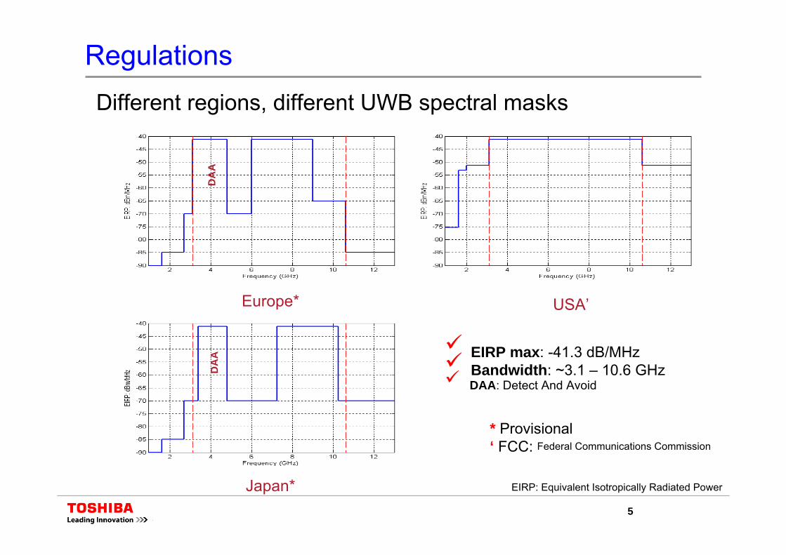
RegulationsDifferent regions, different UWB spectral masks
Europe* USA’
Japan*
DA
AD
AA
Reg
ulat
ions
EIRP max: -41.3 dB/MHzBandwidth: ~3.1 – 10.6 GHzDAA: Detect And Avoid
* Provisional‘ FCC: Federal Communications Commission
EIRP: Equivalent Isotropically Radiated Power

6
Measuring Equipment

7
Types of UWB Sounders
+
8
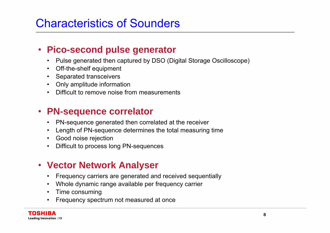
Characteristics of Sounders
• Pico-second pulse generator• Pulse generated then captured by DSO (Digital Storage Oscilloscope)• Off-the-shelf equipment• Separated transceivers• Only amplitude information• Difficult to remove noise from measurements
• PN-sequence correlator• PN-sequence generated then correlated at the receiver• Length of PN-sequence determines the total measuring time• Good noise rejection• Difficult to process long PN-sequences
• Vector Network Analyser• Frequency carriers are generated and received sequentially• Whole dynamic range available per frequency carrier• Time consuming• Frequency spectrum not measured at once

9
UWB Channel Sounding System at TRL
Master controller
Calibration equipment
Channel sounder
Controller forpositioners
Transmit Antenna
Receive Antenna
Positioners
Spectrum analyser
LNA
Bandpass filters
Power amplifiers
LNA: Low Noise Amplifier

10
System Specifications
Sounder type: PN correlation (4095 chips)Bandwidth: ~ 7 GHz (3.5 GHz – 10.5 GHz)Channel snapshots: ~100 per secondMaximum channel length: 589 nsTransmitted Power: ~ 30dBmSpatial channels: 8 (2x4)Antennas: Bi-conical
UWB sounder (MEDAV)

11
Bi-conical Antenna Radiation & VSWR
Radiation at 6.4 GHz
Radiation at 6.4 GHz
Antenna VSWR
Bi-conical antenna (IRK)
Protective casing
VSWR: Voltage Standing Wave Ratio

12
Antenna Gain & Co-polar Power vs. Frequency Antenna Gain
Co-polar power contribution
Calculated from 3D radiation patterns
Measured by the“two-antenna” method*
* C. A. Balanis. Antenna Theory - Analysis and Design. John Wiley & Sons, 1997.
13
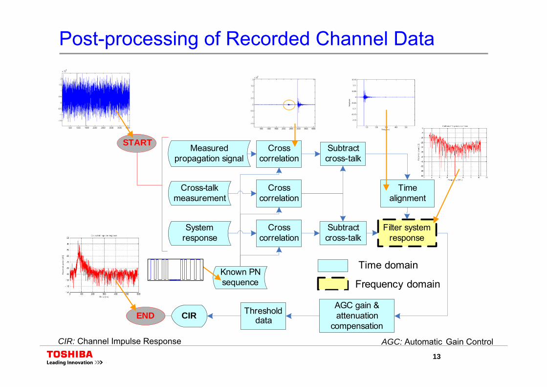
Measured propagation signal
Known PN sequence
System response
Cross-talk measurement
Cross correlation
Cross correlation
Cross correlation
Subtract cross-talk
Subtract cross-talk
Time alignment
Filter system response
CIR Threshold data
AGC gain & attenuation
compensation
Time domain
Frequency domain
START
END
Post-processing of Recorded Channel Data
AGC: Automatic Gain ControlCIR: Channel Impulse Response

14
Comparison of VNA & TD* Sounder Measurements
Tx antenna
Metallic objects
Servo positioner
Rx antenna
Channel sounding equipment
Anechoic chamber
* Time Domain

15
Channel Models and Measurement Example
16
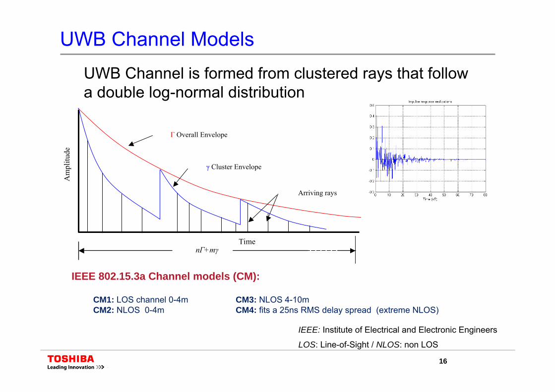
UWB Channel ModelsUWB Channel is formed from clustered rays that follow a double log-normal distribution
CM1: LOS channel 0-4m CM3: NLOS 4-10mCM2: NLOS 0-4m CM4: fits a 25ns RMS delay spread (extreme NLOS)
IEEE 802.15.3a Channel models (CM):
nΓ+mγ
Γ Overall Envelope
γ Cluster Envelope
Am
plitu
de
Time
Arriving rays
IEEE: Institute of Electrical and Electronic Engineers
LOS: Line-of-Sight / NLOS: non LOS

17
Indoor LOS Channel Sounding
Up
3.35m
1.30
m
5
TV
Fireplace
Living room
Kitchen
PC
Hall
Front room
lx0
ky0
kx0 K0
hx0
A
4.15m
1.82
m3.
02m
ly0
lx0L0
fy0
fx0 F0
hy0hx0
H0
B
4
3
2
1
Transmitter location
Receiver location
3.63m
RxØ 0.1 m
Tx
2 m
1.3
m

18
Evidence of New Type of Channel Statistics
PL
δ
Num
ber o
f occ
urre
nces
Slope exponent [δ]
Frequency [GHz]
Mag
nitu
de [d
B]
Mag
nitu
de [d
B]
Frequency [GHz]
2( )PL f f δ−∝Model:
f
Pathloss
Frequency
Frequency path-loss exponent
Extreme exponents can arise!
Width: diffraction?
Shift: reflection, absorption?
19
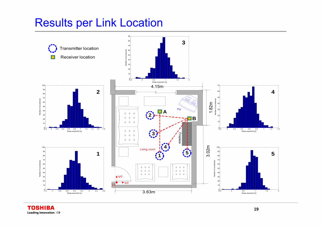
Results per Link Location
Transmitter location
Receiver location
-0.5 0 0.5 1 1.5 20
10
20
30
40
50
60
70
80
90
100
Num
ber o
f occ
urre
nces
Slope exponent [δ]
-0.2 0 0.2 0.4 0.6 0.8 1 1.2 1.40
10
20
30
40
50
60
70
Num
ber o
f occ
urre
nces
Slope exponent [δ]
-0.5 0 0.5 1 1.5 20
10
20
30
40
50
60
70
80
90
Num
ber o
f occ
urre
nces
Slope exponent [δ]
-0.2 0 0.2 0.4 0.6 0.8 1 1.2 1.4 1.6 1.80
10
20
30
40
50
60
70
80
90
100
Num
ber o
f occ
urre
nces
Slope exponent [δ]
-1.2 -1 -0.8 -0.6 -0.4 -0.2 0 0.2 0.40
10
20
30
40
50
60
70
80
90
100
Num
ber o
f occ
urre
nces
Slope exponent [δ]
5
TV
Fireplace
Living room
A
4.15m
1.82
m3.
02m
ly0
lx0
B
4
3
2
1
L0
3.63m
1
2
3
4
5

20
Results and Comparison with Other Measurements
Frequency Path Loss Exponent
Links
Tx Rx
1 A 0.55 ± 0.55
2 B 0.39 ± 0.51
3 B 0.64 ± 0.49
4 B 1.09 ± 0.54
5 B 0.58 ± 0.35
1m reference 0 ± 0.02
All IRs 0.66 ± 0.55
( )δ σ±RMS Delay Spread (ns)
Links
Tx Rx
1 A 6.60 ± 0.87
2 B 5.05 ± 1.32
3 B 6.26 ± 1.31
4 B 8.29 ± 1.18
5 B 8.04 ± 1.641m reference 3.65 ± 0.02
All IRs 6.85 ± 1.62
( )RMSτ σ±
[Malik: 2006] 0.51 ± 0.24 (horizontal) & 0.60 ± 0.20 (vertical)[Chong: 2005] 0.62 ± 0.14
Sanity check results:
21
0 2 4 6 8 10 12 14 16 18 2010
-3
10-2
10-1
100
SNR (dB)
PE
R
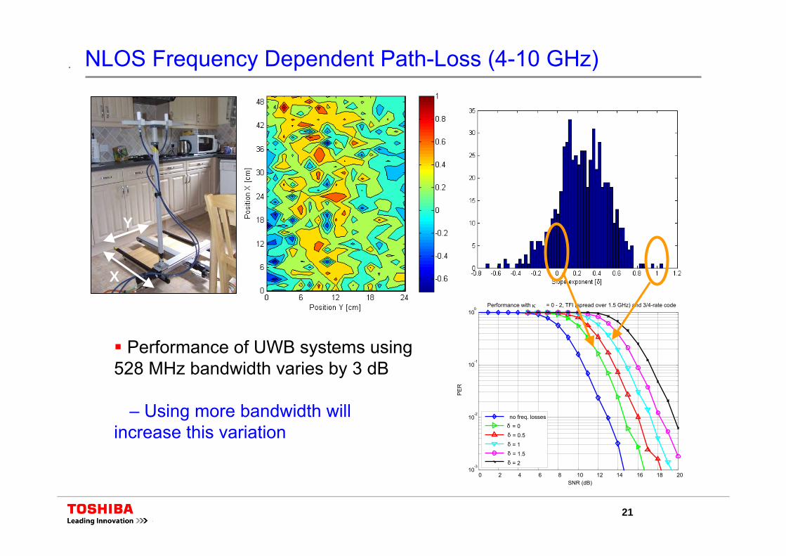
Performance with κ = 0 - 2, TFI (spread over 1.5 GHz) and 3/4-rate code
no freq. lossesδ = 0δ = 0.5δ = 1δ = 1.5δ = 2
NLOS Frequency Dependent Path-Loss (4-10 GHz)
Performance of UWB systems using 528 MHz bandwidth varies by 3 dB
– Using more bandwidth will increase this variation
X
Y

22
Ray Tracing (deterministic) Tools
Characterisation of the radio channel is essential for UWB system design, as pathloss is critical
Antenna radiation patterns measured in anechoic chamber
Mod
ellin
g
Modern house

23
Summary and Conclusions
Brief introduction to UWB and measuring equipment;
State-of-the-art equipment;
Two contrasting sounding techniques;
Channel models and measurement campaign;
Alternative techniques to physical measurements.