the matrix dependent solubility and speciation of …137047/fulltext01.pdf · the matrix dependent...
TRANSCRIPT

1
Örebro University, HT05 Department of Natural Sciences Chemistry D, project work, 20 points
The matrix dependent solubility and speciation of mercury
Erik Hagelberg 760924-6637

2
Table of contents page:
1. Sammanfattning………………………………………………………………... 4
2. Summary………………………………………………………………….……. 5
3. Introduction……………………………………………………………….……. 6
4. Materials and methods………………………………………………….……… 7-11
4.1 Materials……………………………………………………………….. 7
4.1.1 The Solubility Experiments……………………………….………….. 8
4.1.2 The speciation……….………………….…………………..………... 8-9
4.2 Methods……………………………………...……………….………… 9-10
4.2.1 Sample preparation procedure……………………………………….. 8
4.2.2 The speciation method………………………………………………... 9
4.2.3 Adjusting and verifying the speciation method………………………. 10
4.2.4 Instrumentation………………………………………………………. 11
5. Results and discussion…...…………………………………………………….. 12-21
5.1 The mass balance of the speciation method..……….………………….. 12
5.2 Performance comparison of the matrices….…………..……….……… 13
5.3 Effects of time on solubility……………………………………………... 14
5.4 Effects of pH and ionic strength on solubility..…..………..…………… 15-18
5.5 Effects of the Hg0/solution ratio on solubility…….……………………. 19-20
5.6 Interference of volatile nitrogen oxides………………………………… 20-21
6. Conclusions…………………………………………………………………….. 21
7. Acknowledgements…………………………………………………………….. 22
8. References………………………………………………………………..…….. 22

3
Appendix list
Appendix A - Mercury solubility and speciation in matrix L1-L3, 0.74g Hg0/l
Appendix B - Mercury solubility and speciation in matrix L1-L3, 7.4g Hg0/l
Appendix C - Mercury solubility and speciation in matrix L1-L3, 84g Hg0/l
Appendix D - Solubility of Hg0
aq
Appendix E - The effect of pH on the solubility of Hg0
aq
Appendix F - The effect of conductivity on the total solubility of Mercury
Appendix G - The effect of pH on the total solubility of Mercury
Appendix Y – Cement characterization
Appendix Z – Scheme for mercury speciation
4
1. Sammanfattning
Det har beslutats av regeringen att senast år 2010 skall kvicksilverhaltigt avfall med en
kvicksilverhalt på mer än 0.1% slutförvaras i en stabiliserad from djupt ner i berggrunden.
I en doktorsavhandling som genomförts på SAKAB AB i Kumla har det konstaterats att
det är möjligt att överföra elementärt kvicksilver till cinnober, den stabila sulfidformen av
kvicksilver som för övrigt är ett naturligt förekommande mineral. Experiment som pågått
under lång tid för att studera det elementära kvicksilvrets diffusion under olika
omständigheter har också utförts. De uppmätta halterna i vattenfasen har varierat mycket,
från 0.05 till 5 µmolL-1. Det är vad som ligger till grund för det här arbetet.
För att kvicksilvers löslighet skall kunna studeras fullt ut har en specierings metod
vidareutvecklats och verifierats att den fungerar. Studien innefattar hur lösligheten av
kvicksilver påverkas av olika parametrar, som till exempel; matriser med olika egenskaper
och olika kvicksilver/vatten kvoter, samt hur fördelningen mellan oxiderade species och
det elementära kvicksilvret är i vattenfasen (Hg0aq). Den totala lösligheten av kvicksilver
beror dels av matrisens egenskaper och mängden kvicksilver i förhållande till mängden
vätska. Lösligheten av Hg0aq är inte lika beroende av matrisen som de oxiderade species.
Däremot finns trender som visar att högre Hg0/lösning kvot bidrar till en aningen högre
löslighet av Hg0aq. Tid, konduktivitet, pH och omrörning spelar stor roll för vilken
totalhalt och hur stor andel oxiderade species man får i vattenfasen. Lösligheten av Hg0aq,
efter 18 timmar, varierar mellan 0.2 till 0.7 µmolL-1, beroende på Hg0/lösning kvoten.
Efter 18 timmar är lösligheten för de oxiderade species mycket mer varierande, från 0.1
till 28.6 µmolL-1. Detta beror bland annat på att matrisens sammansättning och redox-
potential spelar en viktig roll för vilka komplex som kan bildas med kvicksilverjonerna
och på så sätt bidra till en ökad löslighet.

5
2. Summary
The Swedish government has decided that waste containing more than 0.1% mercury is to
be placed in a permanent repository in the bedrock1,10. To minimize the risk of spreading
mercury, elemental mercury must first be converted into a practically insoluble
compound. In a PhD investigation of stabilization attempts at SAKAB AB in Kumla
favorable conditions for conversion of mercury to cinnabar (the sparingly soluble sulphide
form of mercury and the naturally occurring mineral) was found. In a long-term study of
diffusion of mercury it was found that water solubility of mercury varied much, from 0.05
to 5 µmolL-1.
To be able to study the water solubility of mercury as detailed as possible a speciation
method was developed and verified. This investigation includes how different parameters,
like matrix properties and Hg0/solution ratios effects the solubility of mercury and how the
different species are distributed in the water phase. The total solubility of mercury is very
dependent of both the matrix properties and the Hg0/solution ratio.
Aqueous elemental mercury (Hg0aq) is not as matrix dependent as the oxidized species.
However, trends show that a higher Hg0/solution ratio contributes to a higher solubility of
Hg0aq. Factors like time, pH, ionic strength and degree of stirring, greatly effects the total
solubility of mercury. The concentration of the oxidized mercury species generated from
elemental mercury increases over time and is very dependent on the properties of the
matrix. After 18 hours the solubility of Hg0aq ranges from 0.2 to 0.7 µmolL-1, depending
on Hg0/solution ratio. The solubility for the oxidized species has a much larger variation,
ranging from 0.1 to 28.6 µmolL-1. Among other things, because the composition and
redox potential of the matrix plays an important role in what mercuric complexes can be
expected to form, and contribute to the solubility.

6
3. Introduction
Mercury is known to be one of the most toxic pollutants. It bioaccumulates and can be
converted to even more toxic forms e.g. methylmercury. The Swedish government has
decided that waste containing more than 0.1% mercury is to be placed in a permanent
repository in the bedrock1,10. To minimize the risk of spreading mercury, elemental mercury
must first be converted into a practically insoluble compound. In a PhD investigation of
stabilization attempts at SAKAB AB in Kumla, a favorable condition for conversion of
mercury to cinnabar (the sparingly soluble sulphide form of mercury and the naturally
occurring mineral) was found. In a long-term study of diffusion of mercury it was found that
water solubility of mercury varied much, from 0.05 to 5 µmolL-1. Others have previously
studied the solubility of elemental mercury in distilled water. Publications by Amyot et. al3
and Feng et. al4. reports a solubility of 0.2 µmolL-1 at 20°C and 21°C respectively, which
corresponds to a concentration of about 0.3 µmolL-1 at 25°C. In other studies, performed at
25°C, similar solubility of mercury was found; Budavari et. al11, 0.28 µmolL-1, Canela et. al6,
0.3 µmolL-1 and Clever et. al2 reports a value of about 0.30 ± 0.012 µmolL-1 as a
recommended value at 25°C, based on an average of six external studies. Canela et. al6 also
studied the effect of different Hg0/solution ratios, (10 and 100 g L-1) their results reinforced
the theory that the surface area of the mercury droplet controls the reactive dissolution process
of elemental mercury. It has been verified in recent investigations by Amyot et.al3, that the
surface area of the mercury droplet plays an important role of the dissolution process.
The purpose of this work is to study the solubility of elemental mercury in three different
liquid matrices and at three different mercury/solution ratios. The investigation includes how
different parameters (time, pH, conductivity, mercury/solution ratio) effect the distribution of
oxidized species and Hg0aq. To accomplish this a speciation method was evaluated and
verified.

7
4. Materials and Methods
4.1 Materials
4.1.1 The Solubility Experiments
Three liquid matrices were prepared for the solubility experiments, L1, L2 and L3 numbered
by increasing ionic strength. Matrix L1 was prepared to the concentration of 1 mmolL-1 NaCl
and 1 mmolL-1 NaHCO3 in Milli-Q water (18M Ωcm). L2 was prepared in the same way as
L1 but with the addition of 1.8 mmol concentrated H2SO4 per liter and subsequent boiling to
achieve equilibrium of the CO2 - H2O -system. The third matrix, L3, was prepared by
leaching of crushed concrete. A concrete slab was prepared by mixing 300 grams concrete
(Finbetong, 12104625, Optiroc) with 45 grams tap water. The one centimeter thick concrete
slab was set to harden in a covered plastic box for one week at an ambient temperature of
20°C. After one week the slab was crushed and leached in Milli-Q water for one week and
then filtrated through a polycarbonate filter (Ø=0.40µm, Osmonics). The hardened concrete
and Milli-Q water was mixed in a liquid/solid ratio of 10. Conductivity and pH was measured
in the three matrices, see table 4.1.1.
Table 4.1.1 Matrix measurements (25°C)
Matrix pH Conductivity (mSm-1
)
L1 8.3 20 L2 2.6 120 L3 12.4 490
All chemicals used in experiments and analyses were of pro analysi grade (Merck) with the
exception of KMnO4 (technical quality) and the elemental mercury, which was taken from
encapsulated thermometers and manometers. All of the experiments and analyses were
performed at an ambient temperature of 20°C. The matrices and solutions used in the
experiments were spiked with mercury standard to control how they performed during
analysis.

8
4.1.2 The speciation
For the speciation two different trapping solutions were prepared. A KCl solution consisting
of 10 mmolL-1 KCl and 0.6 mmolL-1 HCl and a KMnO4 solution consisting of 17 mmolL-1
KMnO4 and 500 mmolL-1 H2SO4. The first for trapping potential evaporated ionized mercury
from the sample and the second for trapping the elemental mercury evaporated from the
sample.
4.2 Methods
4.2.1 Sample preparation procedure
The solubility experiments were carried out in 50ml Sartedt tubes (PP) in the three different
matrices, with three different Hg0/solution ratios (0.74;7.4 and 84) and with four different
running times 1, 3 ,10 and 18 hours. 50.00 grams of matrix was weighed in the tube and
elemental mercury was transferred with pipette. The tube was covered with aluminum foil to
reduce the influence of any photoinduced redox processes3,5 and placed in a overhead mixer
(Heidolph, Reax 2) to shake slowly (20 r.p.m). After completed running time, 30 ml of the
sample liquid was carefully transferred to another 50 ml Sarstedt tube with a 5 ml pipette.
Care was taken to only transfer the upper layer of the liquid, to avoid any accidental pickup of
elemental mercury. Also, care was taken not to blow bubbles with the pipette and thereby
purge some of the dissolved elemental mercury (Hg0aq) from the water phase. A portion of the
non-purged sample solution was oxidized with one drop of KMnO4 (5%) and after analysis
referred to as total mercury (HgTOT). A schematic for the speciation method described above
is available in appendix Z.

9
N2 (g)
3 1 2
4.2.2 The speciation method
The speciation of mercury was performed with a purge and trap method. The Hg0
aq was
purged with nitrogen gas from the sample solution, through a trap for volatile ionized mercury
species and finally trapped in an oxidative solution. An equipment
like the schematic in figure 4.2.2 was constructed from three 15ml
Sarstedt tubes and PTFE tubing (Ø=4mm outer diameter and 1 mm
inner diameter) was used for the connection between the tubes.
The PTFE tubing was cut to the same length and adjusted to have
equal clearance from the tube bottom (1 cm). A round hole was cut
in the screw cap and re-plugged with a silicone plug which
previously had two holes drilled in it.
Figure 4.2.2. Schematic of speciation equipment.
The screw caps and the PTFE tubing was acid washed (10%-vol HNO3) overnight and
thoroughly rinsed with Milli-Q and dried with compressed air prior to use. A new set of
Sarstedt tubes was used for each speciation. Tube 1 (figure 4.2.2) was filled with 7 ml sample
solution, tube 2 with 7 ml KCl solution and tube 3 was filled with 7 ml KMnO4 solution
which was centrifuged for 4 minutes at 4000 r.p.m prior to use, to avoid the interference of
any precipitated MnO2.
After speciation, tube 1 was expected to contain ionized mercury species that are dissolved in
the water phase, tube 2 evaporated ionized mercury if any, and tube 3 was expected to contain
the evaporated elemental mercury from the initial solution sample in tube 1. The use of a Y-
connector from the nitrogen supply made it possible to run two replicates at the same time.
The nitrogen flow was controlled regularly and maintained at 100 ml/minute. Prior to
analysis, all samples were preserved with one drop each of HCl and KMnO4 (5%).

10
4.2.3 Adjusting and verifying the speciation method
The speciation method was verified by using a sample, with a known concentration of Hg(II)
(0.5µmolL-1) and HCl (0.12 molL-1). This sample was poured in tube 1 (figure 4.2.2) and
reduced with 10µl SnCl2 (0.1 molL-1), which was added by a droplet that was blown down the
tube wall into the sample with the nitrogen gas. After a couple of test runs it was obvious that
some parameters had to be adjusted to get the method to work properly. For instance, the
initial concentration of KCl in tube 2 (figure 4.2.2) was prepared to a concentration of 0.1
molL-1. After some experiments it was evident that the chloride concentration was too high,
since about 30% of the sample was caught in tube 2. It was suspected that the relatively high
concentration of chlorides combined with the low pH caused oxidation of Hg0aq. Lowering the
concentration to 0.01 molL-1 gave near a total transfer to the trapping solution in tube 3 and no
mercury was detected in tube 2.
It was also observed that the initially used trapping solution (50 mmolL-1 KMnO4) reduced the
signal, likely due to a surplus of MnO4-, since the mixture leaving the reaction manifold on
the FIAS still had a faint purple color. This was simply corrected by preparing a more dilute
solution of KMnO4 (17 mmolL-1), which still is a very large surplus compared to the amount
of mercury. It was also verified that no transfer of mercury occurred when no reducing agent
was added to the sample of known concentration of Hg(II).
11
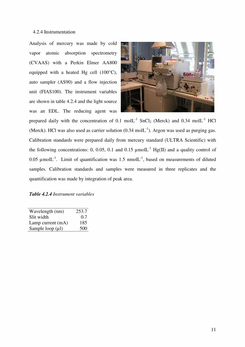
4.2.4 Instrumentation Analysis of mercury was made by cold
vapor atomic absorption spectrometry
(CVAAS) with a Perkin Elmer AA800
equipped with a heated Hg cell (100°C),
auto sampler (AS90) and a flow injection
unit (FIAS100). The instrument variables
are shown in table 4.2.4 and the light source
was an EDL. The reducing agent was
prepared daily with the concentration of 0.1 molL-1 SnCl2 (Merck) and 0.34 molL-1 HCl
(Merck). HCl was also used as carrier solution (0.34 molL-1). Argon was used as purging gas.
Calibration standards were prepared daily from mercury standard (ULTRA Scientific) with
the following concentrations: 0, 0.05, 0.1 and 0.15 µmolL-1 Hg(II) and a quality control of
0.05 µmolL-1. Limit of quantification was 1.5 nmolL-1, based on measurements of diluted
samples. Calibration standards and samples were measured in three replicates and the
quantification was made by integration of peak area.
Table 4.2.4 Instrument variables
Wavelength (nm) 253.7 Slit width 0.7 Lamp current (mA) 185 Sample loop (µl) 500

12
5. Results and discussion
5.1 The mass balance of the speciation method
The mass balance was
calculated from the sums of
mercury contents in tube 1,
tube 2 and tube 3 divided by
the concentration of total
mercury in the initial sample.
The median of the mass
balance was 95.7%. As
visualized in the histogram in figure 5.1 the distribution of the mass balance has a negative
skew that reduces the mean (91.7%) of the mass balance. In some of the speciation
experiments there were considerable losses of mercury, since a mass balance of only 68% was
achieved. This was measured especially in the experiments with the smallest amount of
elemental mercury and in the matrix with lowest ionic strength (L1). Since the major
contributor to total mercury solubility during these conditions is Hg0aq (53-77%) it seems
plausible to assume that some of the Hg0aq was evaporated or absorbed by the plastic tubes.
To control if the polypropylene test tubes used for the speciation experiments did absorb
mercury, a qualitative test was performed. One of the used test tubes from the solubility
experiments were rinsed thoroughly with Milli-Q water 4 times and filled with concentrated
HCl. After three hours of leaching, the acid solution measured about 1 µmolL-1. Even though
not controlled in the speciation experiments, considerable amounts of mercury are in fact
absorbed by the test tubes. To maximize the recovery one should consider using glassware
instead of plastic since it does not absorb mercury.
Massbalance (%)
Frequ
en
cy
110100908070
12
10
8
6
4
2
0
Mean 91,71
StDev 10,51
N 36
Histogram of MassbalanceNormal
Figure 5.1 Histogram of massbalance in the speciation experiments, md = 95.7%

13
5.2 Performance comparison of the matrices
As mentioned earlier (chapter 4.1.1)
the three matrices used in the
solubility experiments were spiked
with equal amount of Hg2+ standard
to ensure that the measurements
would not differ too much because of
different matrix composition. Figure
5.2 visualizes the relative difference between measurements in the three matrices.
A maximum of 2.3% in difference was observed between the matrices. Hence, such a small
difference can be neglected when comparing the solubility experiments, since the difference
in solubility between matrices is in most cases of several magnitudes. Figure 5.3 shows the
variation in precision of the
spiked matrices. The variation in
precision can also be neglected,
since the largest variation is
1.92*10-3 µmolL-1 (Milli-Q).
Matrix
Rela
tive
con
cen
trati
on
(%
)
L3L2L1MQ
100
95
90
85
80
Figure 5.2 Relative comparison of spiked matrices, with spiked Milli-Q as reference (100%)
Chart: Matrix vs Relative concentration
Matrix
[Hg
] (µ
mol/
L)
L3L2L1MQ
0,0525
0,0520
0,0515
0,0510
0,0505
0,0500
Interval plot: Matrix vs concentration
Figure 5.3 Spiked matrices. Comparison of variation in precision.
95% CI for the Mean, n=3

14
5.3 Effects of time on solubility
The total solubility of mercury increases as a
function of time, similar to the appearance in
figures 5.4 and 5.5 (for all graphs, see
Appendix A-C). In general, the major
contributor to solubility is the oxidized
species continuously generated from
oxidation of the elemental mercury. The
experiment with the combination of matrix
L2 and Hg0/solution ratio 7.4 deviates from the other experiments. When examining figure
5.5, it looks like HgTOT has come to a steady state. After 10 hours it was observed that the
surface of the mercury droplet had gone from shiny metallic to a dull gray. Amyot et. al3
reports similar results and hypothesized that the oxidation of the surface of the mercury
droplet is limiting further oxidation. Matrix L2 has a low pH (2.6) and due to a moderate ionic
strength and the presence of oxygen, the matrix can be considered to have a high pe. The
compound formed on the surface of the metallic mercury was probably Calomel (Hg2Cl2),
which can form under certain circumstances (see Pourbaix diagram figure 5.6). It seems
plausible that the layer of calomel could possibly, at least partially, isolate the surface from
the surrounding solution and inhibit the dissolution process. Overall, after 18 hours, the
solubility of Hg0aq ranged from 0.2 µmolL-1
to 0.7 µmolL-1. The total solubility had a
much large range, from 0.1 to 28.6 µmolL-1,
depending on the choice of matrix and
Hg0/solution ratio. Oxidized mercuric species
continues to increase over time and to a
greater extent in matrices with a high ionic
strength.
Time (h)
[Hg
] (µ
mol
/L)
181031
5
4
3
2
1
0
L2M HgTOT
L2M Hg2+
L2M Hg0
Variable
Mercury solubility / speciation in matrix L2, 7.4 g Hg(0)/l
Figure 5.5 Mercury concentration and speciation vs Time
Time (h)
[Hg
] (µ
mol/
L)
181031
5
4
3
2
1
0
L3S HgTOT
L3S Hg2+
L3S Hg0
Variable
Figure 5.4 Mercury concentration and speciation vs Time
Mercury solubility / speciation in matrix L3, 0.74 g Hg(0)/l

15
5.4 Effects of pH and ionic strength on solubility
Mercury solubility was studied in three
different matrices with different pH; 8.3, 2.6
and 12.4. The total solubility of mercury is
always highest at pH 12.4 and, in general,
lowest at pH 8.3 (see figures 5.7-5.9 or
appendix G). Canela et. al6 observed in their
studies of the pH dependency of mercury
solubility, that at pH 7 and 9 the dominating
specie is Hg0aq. They found, that in solutions
with pH 7 and 9 the solubility of Hg0aq
accounts for 74% and 58%, respectively, of the total mercury solubility. When combining
matrix L1 (pH 8.3) with the Hg0/solution ratio of 0.74, the dominating specie is Hg0aq
(see
figure 5.10) with a range from 53% to 77% of the mercury total, depending on time of
measurement.
pH
[Hg
] (µ
mol/
L)
12,48,32,6
5
4
3
2
1
0
1H
3H
10H
18H
Variable
Total solubility of Mercury vs pH, 0.74 g Hg(0)/L
Figure 5.7 Total solubility of Mercury vs pH, at different points in time.
pH
[Hg
] (µ
mol/
L)
12,48,32,6
30
25
20
15
10
5
0
1HM
3HM
10HM
18HM
Variable
Total solubility of Mercury vs pH, 7.4 g Hg(0)/L
Figure 5.8 Total solubility of Mercury vs pH, at different points in time.
pH
[Hg
] (µ
mol/
L)
12,48,32,6
30
25
20
15
10
5
0
1H
3H
10H
18H
Variable
Total solubility of Mercury vs pH, 84 g Hg(0)/L
Figure 5.9 Total solubility of Mercury vs pH, at different points in time.
Time (h)
[Hg
] as
µm
ol/
L
181031
0,4
0,3
0,2
0,1
0,0
L1S HgTOT
L1S Hg2+
L1S Hg0
Variable
Solubility and speciation in matrix L1 vs Time, 0.74g Hg(0)/L
Figure 5.10 Hg(0), the dominating specie
Figure 5.6 Pourbaix diagram of some Hg species

16
A lowered pH increases the redox potential and should thus increase the oxidation rate of Hg0
to Hg(I) and Hg(II). According to the Pourbaix diagram in figure 5.4 the dominating species
at pH < 3.6 and high pe and are Hg(I) and Hg(II). Comparing matrix L2 (pH 2.6) with matrix
L1 (ph 8.3) there is a promoted oxidation which probably is due to the lowered pH (figures
5.7, 5.9). As mentioned earlier, due to oxide buildup on the surface of the elemental mercury,
the same trend is not present when combining matrix L2 and Hg0/solution ratio of 7.4 (figure
5.8). In matrix L1 (pH 8.3) the solubility is suppressed in comparison with the others, this is
expected, since the pH is slightly alkaline oxidation should not be the favorable. The anions
chloride, hydroxide and carbonate are all known to be good complex formers in conjunction
with mercury13 and at pH 8.3 the concentrations of hydroxide and caronate are too low
([OH-] ≈ 2 µmolL-1 @ pH 8.3) to make an impact on the solubility through formation of
complexes. However in matrix L3 (pH 12.4) a solubility maximum was observed in all cases.
This is difficult to explain only in terms of pH and is probably a due to the fact that at pH 12.4
the concentrations of hydroxide and carbonate are high ([OH-] ≈ 25 mmolL-1 @ pH = 12.4)
and that forming Hg-complexes would shift the equilibrium (Hg0 ↔ Hg2+) to the right and
thus withdrawing free Hg2+.
Yamamoto et. al9 reports that the presence of molecular oxygen combined with halogens, like
chloride and iodide stimulates the oxidation of elemental mercury in a linear fashion. Even
though the presence of chlorides probably influences the solubility of mercury, it has not been
studied explicit in this work since all the matrices have different compositions. Despite the
fact that the chloride concentrations in matrices L1 and L2 are the same (1 mmolL-1) the total
solubility of mercury is in most cases higher in matrix L2. As H2SO4 was used for
acidification in matrix L2, this is likely an effect of pH since the sulphate is a poor complex
former compared to chloride and carbonate13.

17
Seen from the perspective of ionic
strength, measured as conductivity, the
results are interpreted a little different.
As figure 5.11, 5.12, 5.13 (or appendix
F) illustrates, it looks like increased
conductivity has a positive influence
on the total solubility of mercury, with
the exception of the suppressed
solubility in matrix L2 and
Hg0/solution ratio 7.4 (fig 5.12). But
since the three matrices differ in
composition one cannot simply
determine whether this is a sole effect
of conductivity or just the interaction
between mercury and complex formers
like hydroxide, chloride and carbonate.
Further investigation is necessary to
fully understand how and if ion
strength alone has some central role in
the solubility of mercury. This could
perhaps be accomplished by working
in clean and known matrices and
without known complex formers.
Conductivity (mS/m)
[Hg
] (µ
mol/
L)
49012020
4
3
2
1
0
1HS
3HS
10HS
18HS
Variable
HgTOT vs conductivity, 0.74g Hg(0)/L
Figure 5.11
Conductivity (mS/m)
[Hg
] (µ
mol/
L)
49012020
30
25
20
15
10
5
0
1HM
3HM
10HM
18HM
Variable
HgTOT vs conductivity, 7.4g Hg(0)/L
Figure 5.12
Conductivity (mS/m)
[Hg
] (µ
mol/
L)
49012020
30
25
20
15
10
5
0
1HL
3HL
10HL
18HL
Variable
HgTOT vs conductivity, 84g Hg(0)/L
Figure 5.13

18
When it comes to the solubility of
Hg0aq it is not as matrix dependent
as the oxidized species. In the
experiments with the Hg0/solution
ratio of 0.74 the concentration of
Hg0aq in the three matrices after 18
hours is almost the same (fig.
5.14). In all three matrices the
solubility of Hg0aq were very close
to the literature value3,4 of 0.2
µmolL-1 at 20°C. The experiments
with the higher Hg0/solution ratios
(7.4 and 84) show that the
solubility of Hg0aq has similar
trends (fig. 5.15 and 5.16, or
appendix E) to that of the oxidized
species (fig 5.7-5.9). Even though
the behavior of Hg0aq is not fully
understood during these
conditions, it is possible that the
phenomenon observed in fig 5.15
and 5.16 is due to the fact that the
system has not come to a point
close to equilibrium and that it
would eventually land closer to the expected 0.2 µmolL-1. To achieve an equilibrium the
systems would probably had needed much longer time than 18 hours to stabilize, but given
the limited timeframe of this project this was not possible.
pH
[Hg
] µ
mol/
L
12,48,32,6
1,0
0,8
0,6
0,4
0,2
0,0
1HS
3HS
10HS
18HS
Variable
Hg(0)aq vs pH, 0.74 g Hg(0)/L
Figure 5.14
pH
[Hg
] µ
mol/
L
12,48,32,6
1,0
0,8
0,6
0,4
0,2
0,0
1HM
3HM
10HM
18HM
Variable
Hg(0)aq vs pH, 7.4 g Hg(0)/L
Figure 5.15
pH
[Hg
] µ
mol/
L
12,48,32,6
1,0
0,8
0,6
0,4
0,2
1HL
3HL
10HL
18HL
Variable
Hg(0)aq vs pH, 84 g Hg(0)/L
Figure 5.16

19
5.5 Effects of the Hg0/solution ratio on solubility
The amount of elemental mercury
placed in contact with the solution
does effect the concentration of
oxidized mercuric species. And as
mentioned in the previous chapter it
also seems to have a temporary
effect on the concentration of Hg0aq.
Amyot et al3 also found that the
amount of elemental mercury effects the rate of oxidation but rather using weight for
comparison he used the surface area, which probably is a more suitable parameter for this
kind of comparison. The studies made by Amyot et al3 also showed that removal of the
elemental mercury droplet ceases further oxidation of Hg0aq and keeping the concentrations of
oxidized mercuric species and Hg0aq nearly constant. Apparently the surface of the mercury
droplet itself also plays a key role to catalyzing the solubility process. Despite the small
amount of tests in this investigation, the indication still is that the Hg0/solution ratio is an
important parameter that controls the dissolution of mercury. Due to splitting of the mercury
droplet in the experiments with
Hg0/solution ratio 84, the method
was slightly changed by decreasing
the stirring by changing the type of
mixer (Heidolph Promax,
reciprocating mixer at 100 r.p.m).
Sadly, this is a perfect example of
what happens if experiments are not
completely thought through. Since changed stirring means changed kinetics, comparisons
with the other experiments are now difficult to make. Figures 5.17-5.19 illustrates how the
total solubility of mercury develops over time and how the rate is affected by the amount of
elemental mercury. In matrices L1 and L2 the solubility is considerably lower than expected
Time (h)
[Hg
] µ
mol/
L
181031
10
8
6
4
2
0
L1 HgTOT 0.74g/LL1 HgTOT 7.4g/L
L1 HgTOT 84g/L
Variable
HgTOT vs Time in matrix L1 with different Hg(0)/solution ratios
Figure 5.17
Time (h)
[Hg
] µ
mol
/L
181031
10
8
6
4
2
0
L2 HgTOT 0.74g/L
L2 HgTOT 7.4g/L
L2 HgTOT 84g/L
Variable
HgTOT vs Time in matrix L2 with different Hg(0)/solution ratios
Figure 5.18

20
in the experiments with
Hg0/solution ratio 84, this is likely
due the lower kinetics, as discussed
above. However, in matrix L3 the
total solubility is indeed higher
than that of matrix L3 combined
with Hg0/solution ratio 7.4 (fig
5.19), which could indicate that if
kinetics would have been the same in all of the experiments, a higher solubility might have
been expected. Amyot et. al3 found that the oxidation rate depends on the surface area of the
mercury droplet, but it does not increase by an order of magnitude.
5.6 Interference of volatile nitrogen oxides
Analysis of mercury by
CVAAS is based on the
reduction of oxidized Hg-
species to volatile elemental
mercury. In terms of basic
redox chemistry, there are
several species that can
interfere with the reduction of
Hg and thus give a decrease
in signal. This was observed when verifying the speciation method. Samples with known
Hg(II) content were prepared from Hg standard, then reduced and speciated as described in
chapter 4.2.2. When controlling the known sample, a loss of about 17% was discovered. The
analysis did not measure the expected concentration of 1.25µmolL-1. Preservation and
stabilization of samples (sample volume ~ 7ml) were done with the addition of one droplet of
concentrated HNO3 and one droplet of KMnO4 (5%). Replacing the droplet of HNO3 with
HCl made a significant difference - sample now measured close to the expected 1.25µmolL-1.
Acid used for sample preservation
[Hg
] (µ
mol/
L)
HNO3HCl
1,25
1,03
Interval plot: Comparison of HCl vs HNO3 addition95% CI for the Mean, n=6
Figure 5.20 Comparison of HCl and HNO3 addition as sample preservative
Time (h)
[Hg
] µ
mol/
L
181031
30
25
20
15
10
5
0
L3 HgTOT 0.74g/L
L3 HgTOT 7.4g/L
L3 HgTOT 84g/L
Variable
HgTOT vs Time in matrix L3 with different Hg(0)/solution ratios
Figure 5.19

21
There was not only a gain of signal with HCl addition, the standard deviation between
measurement replicates decreased with a factor of 10 (figure 5.20). This phenomenon,
thought to be caused by volatile nitrogen oxides generated from the reduction of nitrate, has
been observed by Rokkjaer et. al7 when using sodiumtetra-hydroborate for reduction of Hg.
According to a technical report on analysis of mercury in sewage sludge from Perkin Elmer8,
using a SnCl2 solution (0.07 molL-1), no interference from volatile nitrogen oxides could be
found. Perkin Elmer used concentrated aqua regia for sample digestion prior to analysis. In
this work a 0.1 molL-1 SnCl2 solution was used. Rokkjaer et. al7 states that it is likely, that
when using SnCl2 as reducing agent it decreases the risk of interference from nitrogen oxides.
Rokkjaer et. al7 used a SnCl2 solution that had the concentration of 0.44 molL-1 so, clearly, it
seems that the interference of volatile nitrogen oxides are present using a SnCl2 solution with
the concentration of 0.1 molL-1.
6. Conclusions
With a median at 95.7% and an average mass balance of 91.7% the speciation method used in
this work is a simple but effective tool to estimate the fraction of Hg0aq in water samples, at
least in the concentration range in these experiments. All the factors together like time, pH,
ionic strength, Hg0/solution ratio and degree of stirring, greatly affects the total solubility of
mercury. Thus making it difficult to estimate the solubility even in known matrices, or
comparing the results with other studies. The concentration of the oxidized mercury species
generated from elemental mercury increases over time and is very dependent on the properties
of the matrix. To minimize the solubility of mercury, a matrix with a low ionic strength and a
neutral pH should be considered.
Since only one experiment was performed at each unique setup (solution, time etc.) and
plastic containers was used, it would be interesting to repeat the experiments using glassware
and make several replicates of each experiment to be able to estimate the variance. Regarding
mercury analysis with CVAAS one should always be critical to the result of the measurement
if not using a pre-reduction stage or when the redox chemistry of the sample is unknown.

22
7. Acknowledgements
First of all I would like to thank my supervisor Margareta Svensson for valuable tips and
assistance in the laboratory. Carl-Johan Löthgren receives a special “thank you” for your
point of view on things and our very interesting chats in the laboratory. Thanks to Anders
Düker for providing me with the Pourbaix diagram and for brainstorming some issues of
technical matter. And at last, big thanks to the helpful handful of people at SAKAB
production lab, for helping me find the necessary chemicals and hardware needed.
8. References
1.) Sveriges Regering (2001), Kvicksilver i säkert förvar - Slutbetänkande från Utredningen om slutförvaring av kvicksilver,
SOU 2001:85.
2.) Clever H. L, Johnson S. A, Derrick, M. E. (1985), The solubility of mercury and some sparingly soluble mercury salts in water
and aqueous electrolyte solutions. J. Phys. Chem. Ref. Data , 14, pages 631-680.
3.) Amyot M, Morel F. M. and Ariva P. A. (2005), Dark Oxidation of Dissolved and Liquid Elemental Mercury in Aquatic
Environments, Environmental Science and Technology, volume 39, No. 1, pages 110-114.
4.) Feng Y-L, Lam J.W. and Sturgeon R. E. (2004), A novel approach to the estimation of aqueous solubility of some noble metal
vapor species generated by reaction with tetrahydroborate (III), Spectrochimica Acta Part B 59, pages 667-675.
5.) Garcia E, Poulain A. J, Amyot M. and Ariva P. A. (2005), Diel variations in photoinduced oxidation of Hg0 in freshwater,
Chemosphere, Volume 59, Issue 7, pages 977-981.
6.) Canela M. C. and Jardim W.F. (1997), The Fate of Hg0 in Natural Waters, J. Braz. Chem. Soc., vol. 8,No 4, pages 421-426.
7.) Rokkjær I, Hoyer B. and Jensen N. (1993), Interference by volatile nitrogen oxides in the determination of mercury by flow
injection cold vapor atomic absorption spectrometry, Talanta, volume 40, pages 729-735.
8.) Perkin Elmer (2004), Using FIMS to determine Mercury content in sewage sludge, sediment and soil samples, Technical Note
TSAA-48E.
9.) Yamamoto M. (1996), Stimulation of elemental mercury oxidation in the presence of chloride ion in aquatic environments,
Chemosphere, Volume 32, No. 6, pages 1217-1224
10.) Swedish Riksdag Avfallsförorningen, SFS 2001:1063 21c §, http://www.notisum.se/rnp/sls/lag/20011063.htm .
Last visited 2005-10-20
11.) Budavari, S., O'Neil, M.J., Smith, A., Heckelman, P.E. (1989). The Merck Index - an encyclopedia of chemals, drugs, and
biologicals. Rahway, N.J., Merck & Co., USA.
12.) Weast, R.C., Astle, M.J. (1981). CRC Handbook of Chemistry and Physics: a ready-reference book of chemical and physical
data. Cleveland, Ohio: CRC Press, Cop., Ohio.
13.) Ravichandran, M. (2004) Interactions between mercury and dissolved organic matter - a review, Chemosphere, Vol 55, page 323

Appendix A - Mercury solubility and speciation in matrix L1-L3, 0.74g Hg0/l
= HgTOT
= Hg(ox) = Hg
0aq
Mercury solubility / speciation in matrix L3
0
0,5
1
1,5
2
2,5
3
3,5
4
0 1 2 3 4 5 6 7 8 9 10 11 12 13 14 15 16 17 18 19 20
Time (h)
[Hg]
(µ
mol
/l)
Mercury solubility / speciation in matrix L2
0
0,5
1
1,5
2
2,5
3
3,5
4
0 1 2 3 4 5 6 7 8 9 10 11 12 13 14 15 16 17 18 19 20
Time (h)
[Hg]
(µ
mol
/l)
Mercury solubility / speciation in matrix L1
0
0,05
0,1
0,15
0,2
0,25
0,3
0,35
0,4
0 1 2 3 4 5 6 7 8 9 10 11 12 13 14 15 16 17 18 19 20
Time (h)
[Hg]
(µ
mol
/l)

Appendix B - Mercury solubility and speciation in matrix L1-L3, 7.4g Hg0/l
= HgTOT
= Hg(ox) = Hg
0aq
Mercury solubility / speciation in matrix L1
0
1
2
3
4
5
6
7
8
9
10
0 1 2 3 4 5 6 7 8 9 10 11 12 13 14 15 16 17 18 19 20
Time (h)
[Hg]
(µ
mol
/l)
Mercury solubility / speciation in matrix L2, 7.4 g Hg0/l
0
2
4
6
8
10
0 1 2 3 4 5 6 7 8 9 10 11 12 13 14 15 16 17 18 19 20
Time (h)
[Hg]
(µ
mol
/l)
Mercury solubility / speciation in matrix L3
0
5
10
15
20
25
0 1 2 3 4 5 6 7 8 9 10 11 12 13 14 15 16 17 18 19 20Time (h)
[Hg]
(µ
mol
/l)

Appendix C - Mercury solubility and speciation in matrix L1-L3, 84g Hg0/l
= HgTOT
= Hg(ox) = Hg
0aq
Mercury solubility / speciation in matrix L1
0
0,5
1
1,5
2
2,5
3
3,5
4
4,5
5
0 1 2 3 4 5 6 7 8 9 10 11 12 13 14 15 16 17 18 19 20
Time (h)
[Hg]
(µ
mol
/l)
Mercury solubility / speciation in matrix L2
0
0,5
1
1,5
2
2,5
3
3,5
4
4,5
5
0 1 2 3 4 5 6 7 8 9 10 11 12 13 14 15 16 17 18 19 20
Time (h)
[Hg]
(µ
mol
/l)
Mercury solubility / speciation in matrix L3
0
5
10
15
20
25
30
0 1 2 3 4 5 6 7 8 9 10 11 12 13 14 15 16 17 18 19 20
Time (h)
[Hg]
(µ
mol
/l)

Appendix D - Solubility of Hg0
aq
= L1, = L2, = L3
Solubility of Hg0aq, 0.74 g Hg
0/l
0
0,2
0,4
0,6
0,8
1
0 1 2 3 4 5 6 7 8 9 10 11 12 13 14 15 16 17 18 19 20
Time (h)
[Hg]
(µ
mol
/l)
Solubility of Hg0
aq, 7.4 g Hg0/l
0
0,2
0,4
0,6
0,8
1
0 1 2 3 4 5 6 7 8 9 10 11 12 13 14 15 16 17 18 19 20
Time (h)
[Hg]
(µ
mol
/l)
Solubility of Hg0aq, 84 g Hg
0/l
0
0,2
0,4
0,6
0,8
1
0 1 2 3 4 5 6 7 8 9 10 11 12 13 14 15 16 17 18 19 20Time (h)
[Hg]
(µ
mol
/l)

Appendix E - The effect of pH on the solubility of Hg0
aq
Hg0
aq vs pH, 0.74 g Hg0/l
0
0,2
0,4
0,6
0,8
1
2 3 4 5 6 7 8 9 10 11 12 13
pH
[Hg]
(µ
mol
/l) 1h
3h
10h
18h
Hg0
aq vs pH, 7.4 g Hg0/l
0
0,2
0,4
0,6
0,8
1
2 3 4 5 6 7 8 9 10 11 12 13
pH
[Hg]
(µ
mol
/l) 1h
3h
10h
18h
Hg0aq vs pH, 84 g Hg
0/l
0
0,2
0,4
0,6
0,8
1
2 3 4 5 6 7 8 9 10 11 12 13pH
[Hg]
(µ
mol
/l) 1h
3h
10h
18h

Appendix F - The effect of conductivity on the total solubility of Mercury
HgTOT
vs conductivity, 7.4g Hg0/L Matrix
0
5
10
15
20
25
30
0 50 100 150 200 250 300 350 400 450 500
Conductivity (mSm-1)
[Hg]
TO
T (
µm
ol/l
)
1h
3h
10h
18h
HgTOT
vs conductivity, 0.74g Hg0/L Matrix
0
1
2
3
4
5
0 50 100 150 200 250 300 350 400 450 500Conductivity (mSm-1)
[Hg]
TO
T (
µm
ol/l
) 1h
3h
10h
18h
HgTOT
vs conductivity, 84g Hg0/L Matrix
0
5
10
15
20
25
30
0 50 100 150 200 250 300 350 400 450 500
Conductivity (mSm-1)
[Hg]
TO
T (
µm
ol/l
) 1h
3h
10h
18h

Appendix G - The effect of pH on the total solubility of Mercury
HgTOT
vs pH 0.74g Hg0/l
0
1
2
3
4
5
2 4 6 8 10 12pH
[Hg]
(µ
mol
/l) 1h
3h
10h
18h
HgTOT
vs pH 7.4 g Hg0/l
0
5
10
15
20
25
30
2 4 6 8 10 12pH
[Hg]
(µ
mol
/l) 1h
3h
10h
18h
HgTOT
vs pH 84 g Hg0/l
0
5
10
15
20
25
30
2 4 6 8 10 12
pH
[Hg]
(µ
mol
/l)
1h
3h
10h
18h

Appendix Y
CEMENTA AB Telefon 08-625 68 00 Postgiro 245 70-4 Säte Danderyd
Svärdvägen 11 D Fax 08-625 68 98 Bankgiro 640-1459 VAT nr SE556013586401
Box 144 www.cementa.se Bank Svenska Handelsbanken
182 12 Danderyd [email protected] 542 801 108
Appenfdasdf
Typanalys 2004
Byggcement Std PK Slite
CEM II/A-LL 42,5 R
Kemisk analys Tryckhållfasthet
Medelvärde Medelvärde
CaO 61,4 % 1 dygn 22,1 MPa SiO2 18,9 % 2 dygn 34,6 MPa Al2O3 3,9 % 28 dygn 56,2 MPa Fe2O3 2,7 % MgO 2,5 % Na2O 0,19 % K2O 1,0 %
Övriga fysikaliska data
SO3 3,4 % Cl 0,05 % Vattenbehov 27,3 % Vattenlöslig < 2 mg/kg Bindetid 158 min kromat Volymbeständighet 1,2 mm Vithet R46 30,3 % Specifik yta 456 m2/kg Densitet 3067 kg/m3
Övriga upplysningar
Kornstorleksfördelning
Kalksten 12,2 % 125 µm 100 % C3A 4,7 % 63 µm 97,9 % 32 µm 81,0 % 15 µm 51,0 % 8 µm 31,2 % 5 µm 20,4 % 3 µm 11,1 % 2 µm 5,5 % 1 µm 0,52 %

23
Appendix Z - Scheme for mercury speciation
30 ml sample
14 ml sample
16 ml sample
[HgTOT]
speciation
7 ml sample 7 ml KCl 7 ml KMnO4
7 ml KCl 7 ml KMnO4 7 ml sample
[Hg2+] Volatile Hg? [Hg0aq]
Preservation and analysis