Laboratory 1

Index

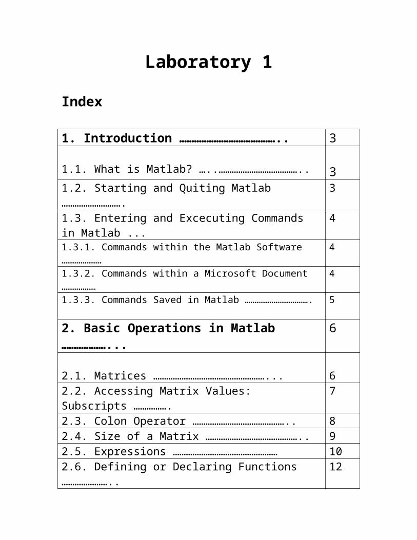
1. Introduction ………………………………….. 3

1.1. What is Matlab? …..……………………………….. 31.2. Starting and Quiting Matlab ………………………. 31.3. Entering and Excecuting Commands in Matlab ... 41.3.1. Commands within the Matlab Software ………………… 41.3.2. Commands within a Microsoft Document ……………… 41.3.3. Commands Saved in Matlab ……………………………. 5

2. Basic Operations in Matlab ………………... 6

2.1. Matrices ……………………………………………... 62.2. Accessing Matrix Values: Subscripts ……………. 72.3. Colon Operator …………………………………….. 82.4. Size of a Matrix …………………………………….. 92.5. Expressions ………………………………………… 102.6. Defining or Declaring Functions ………………….. 122.7. Working with Matrices ……………………………... 132.8. Matrices and Arrays ……………………………….. 142.9. Matrix Transpose Operator ……………………….. 16

3. Graphics ………………………………………. 18

3.1. Plotting Graphs …………………………………….. 183.1.1. Plotting Graphs with Numerical Data: The plot Command ………………………………………………………… 183.1.2. Plotting Graphs Using a Function: The ezplot command …………………………………………………………. 203.1.3. Another Way to Display Graph Output …………………. 22

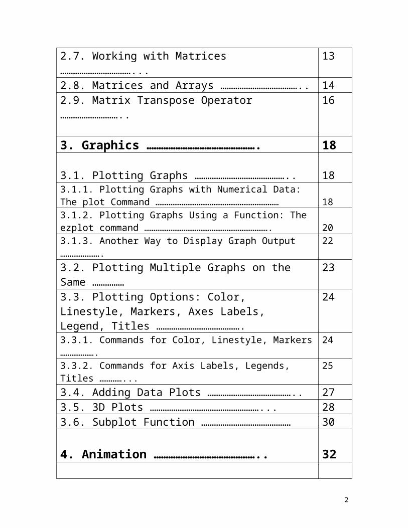
3.2. Plotting Multiple Graphs on the Same …………… 233.3. Plotting Options: Color, Linestyle, Markers, Axes Labels, Legend, Titles ………………………………….

24

3.3.1. Commands for Color, Linestyle, Markers ………………. 243.3.2. Commands for Axis Labels, Legends, Titles …………... 253.4. Adding Data Plots ………………………………….. 273.5. 3D Plots ……………………………………………... 283.6. Subplot Function …………………………………… 30

4. Animation …………………………………….. 32

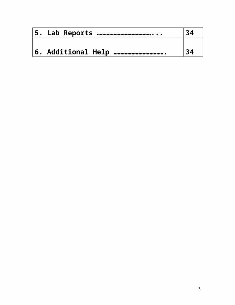
5. Lab Reports …………………………………... 34

6. Additional Help ………………………………. 34

2

1. INTRODUCTION

1.1. WHAT IS MATLAB?

MATLAB is a high-performance language for technical computing. It integrates computation, visualization, and programming in an easy-to-use environment where problems and solutions are expressed in familiar mathematical notation. It is widely used in the sciences, mathematics and engineering.

Typical uses include:

Math and computationAlgorithm developmentModeling, simulation, and prototypingData analysis, exploration, and visualizationScientific and engineering graphicsApplication development, including Graphical User Interface building

MATLAB is an interactive system whose basic data element is an array that does not require dimensioning. This allows you to solve many technical computing problems, especially those with matrix and vector formulations, in a fraction of the time it would take to write a program in a scalar noninteractive language such as C or Fortran.

The name MATLAB stands for matrix laboratory.

MATLAB was originally written to provide easy access to matrix software developed by the LINPACK and EISPACK projects, which together represent the state-of-the-art in software for matrix computation.

1.2. STARTING and QUITING MATLAB

To run MATLAB on a PC, double-click on the MATLAB icon.

To quit MATLAB at any time, type quit at the MATLAB prompt, or from the menu select File->Exit MATLAB.

If you feel you need more assistance, type help at the MATLAB prompt, or pull down on the Help menu on a PC.

3

You want to change the Current Directory listed on the tool bar to your U: drive as this is where you want to save all your work. You can use the icon with the 3 dots (...) to open a browser to select the appropriate directory.

1.3. ENTERING AND EXECUTING COMMANDS IN MATLAB

MATLAB is an interactive computing language. As with any computing or programming language, you enter and execute commands. Commands have a particular syntax, which means things like punctuation, case and symbols are important and you have to pay attention to the way you type things. This is similar to any spoken languge - if the syntax (ie. spelling and grammar) is not correct, then it is difficult to understand what things mean.

There are 3 ways you can enter and execute commands in MATLAB:

1) Start MATLAB and type and execute commands at the MATLAB prompt in the command window.

2) Type commands in a Microsoft Word document that is a MATLAB Notebook and execute the commands within the Notebook. To use this feature you must set up the MATLAB software to work with Microsoft Word. See the handout on MATLAB Notebook for Microsoft Word.

3) Save commands in an M-file (MATLAB file) and execute the M-file from within MATLAB.

1.3.1 COMMANDS within the MATLAB softwareYou type MATLAB commands in the command window at the MATLAB command line prompt, which is denoted by >>. Press Enter or return to execute commands. For example, at the MATLAB prompt type in the following command and press Enter.

1/3 + 1/4

1.3.2 COMMANDS within a Microsoft Word documentIf your Microsoft Word document is a MATLAB Notebook (such as this document), you can type MATLAB commands directly in your Word document and execute them. (A Word document is a MATLAB Notebook if the entry "Notebook" appears on the Word menu bar. An advantage of using the MATLAB Notebook feature is that your MATLAB results or output are embedded directly in your Word document.

4

You enter MATLAB commands in a Word document which is a MATLAB Notebook as follows: type the command and make it a MATLAB input cell by placing your cursor anywhere in the command and from the menu click on Notebook->Define Input Cell. The command will change to a bold, dark green color enclosed within cell markers.

To execute an input cell, just put the cursor on the input cell and press CTRL+Enter.

1/3 + 1/4

ans = 0.5833

See the handout MATLAB Notebook for Miscrosoft Word for more information on entering and executing command in a MATLAB Notebook / Word document.

1.3.3. COMMANDS SAVED in an M-file: Multiple MATLAB commands can be saved in an M-file (MATLAB file). M-files are text files which contain MATLAB code and just contain the same statements you would type at the MATLAB command line. To make it a MATLAB file we add an extension .m to the name. So the file is stored as lab1.m.

You can view the contents of an M-file or create a new M-file by using the MATLAB Editor/Debugger. From the MATLAB toolbar, select File->New->M-file or File->Open to create/open a file in the debugger. By using File->Save you can save the contents of an M-file. Make sure that the file name ends in .m!

To write text or comment a line in a M-file you need to use a percentage sign (i.e. % ) in front of it. Alternatively, you can type your lines of text, select/highlight them using the left mouse button, and then select Comment from the Text menu.

A comment symbol, %, is added at the start of the selected lines. The lines that do not have a percentage sign in front of it are commands in MATLAB that can be executed.

To execute or see the output of an M-file you need to enter the file name without the .m extension at the MATLAB prompt in the command window. For example, simply enter lab1 at the MATLAB prompt to execute this file.

You can interrupt a running program by pressing Ctrl+C or Ctrl+Break at any time.

5

2. BASIC OPERATIONS IN MATLABAs you have seen, some commands are just like you would type things in a calculator.

If you want to refer the result of the command, you need to give it a name, or in other words, assign the result to a variable. The following command assigns the result to the variable s.

s = 1/3 + 1/4

s = 0.5833

If a command does not fit on one line, use an ellipsis (three periods), ..., followed by Return/Enter to indicate that the statement continues on the next line. For example,

s = 1 - 1/2 + 1/3 -1/4 + 1/5 - 1/6 + 1/7 ...- 1/8 + 1/9 - 1/10 + 1/11 - 1/12

s = 0.6532

2.1. MATRICES

MATLAB uses matrices to store and manipulate data. A matrix is a rectangular array of numbers (ie. numbers arranged in rows and columns).

Special meaning is sometimes attached to 1-by-1 matrices, which are called scalars, and to matrices with only one row or column, which are called vectors. MATLAB has other ways of storing both numeric and nonnumeric data, but in the beginning, it is usually best to think of everything as a matrix.

The operations in MATLAB are designed to be as natural as possible. Where other programming languages work with numbers one at a time, MATLAB allows you to work with entire matrices quickly and easily.

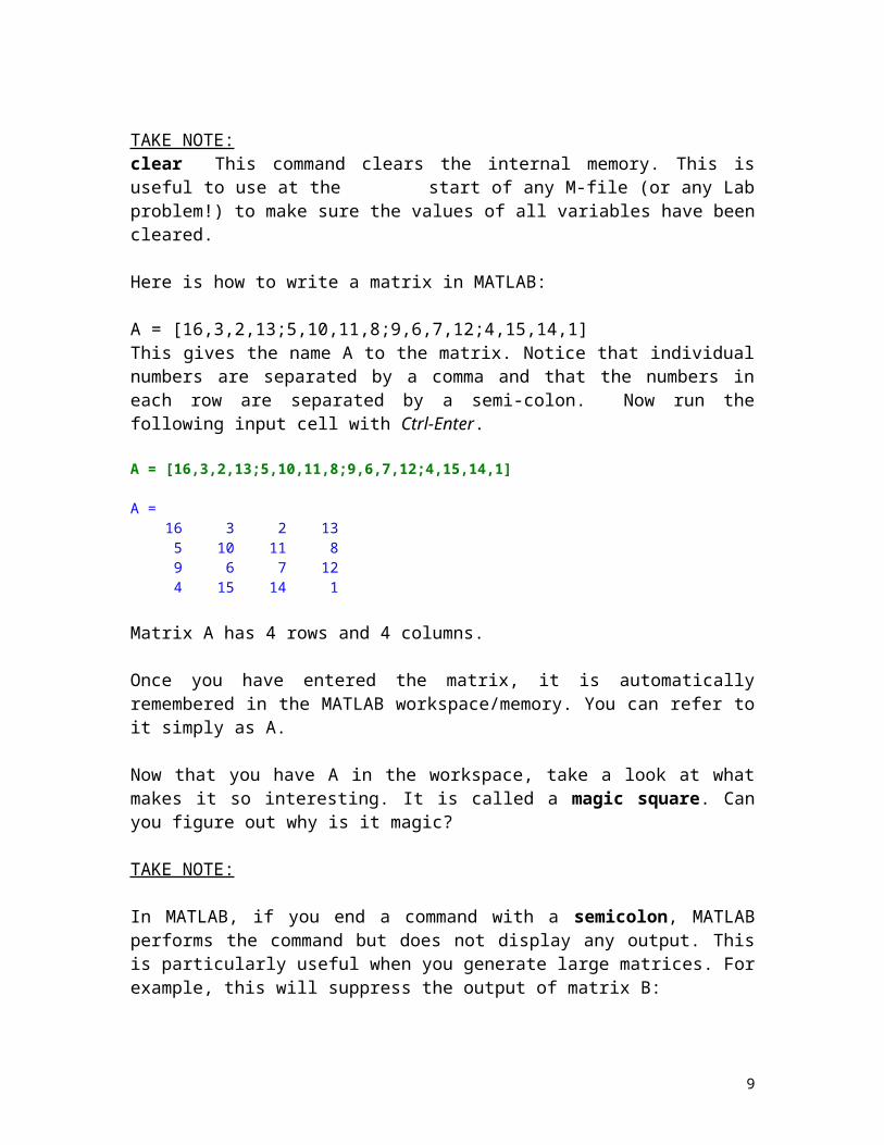
TAKE NOTE:clear This command clears the internal memory. This is useful to use at the start of any M-file (or any Lab problem!) to make sure the values of all variables have been cleared.

Here is how to write a matrix in MATLAB:

A = [16,3,2,13;5,10,11,8;9,6,7,12;4,15,14,1]

6

This gives the name A to the matrix. Notice that individual numbers are separated by a comma and that the numbers in each row are separated by a semi-colon. Now run the following input cell with Ctrl-Enter.

A = [16,3,2,13;5,10,11,8;9,6,7,12;4,15,14,1]

A = 16 3 2 13 5 10 11 8 9 6 7 12 4 15 14 1

Matrix A has 4 rows and 4 columns.

Once you have entered the matrix, it is automatically remembered in the MATLAB workspace/memory. You can refer to it simply as A.

Now that you have A in the workspace, take a look at what makes it so interesting. It is called a magic square. Can you figure out why is it magic?

TAKE NOTE:

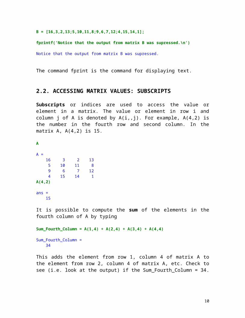
In MATLAB, if you end a command with a semicolon, MATLAB performs the command but does not display any output. This is particularly useful when you generate large matrices. For example, this will suppress the output of matrix B:

B = [16,3,2,13;5,10,11,8;9,6,7,12;4,15,14,1];

fprintf('Notice that the output from matrix B was supressed.\n')

Notice that the output from matrix B was supressed.

The command fprint is the command for displaying text.

2.2. ACCESSING MATRIX VALUES: SUBSCRIPTS

Subscripts or indices are used to access the value or element in a matrix. The value or element in row i and column j of A is denoted by A(i,,j). For example, A(4,2) is the number in the fourth row and second column. In the matrix A, A(4,2) is 15.

A

A = 16 3 2 13 5 10 11 8 9 6 7 12 4 15 14 1

7

A(4,2)

ans = 15

It is possible to compute the sum of the elements in the fourth column of A by typing

Sum_Fourth_Column = A(1,4) + A(2,4) + A(3,4) + A(4,4)

Sum_Fourth_Column = 34

This adds the element from row 1, column 4 of matrix A to the element from row 2, column 4 of matrix A, etc. Check to see (i.e. look at the output) if the Sum_Fourth_Column = 34.

Here are some MATLAB commands which this lab uses to control the outputof the M-file.

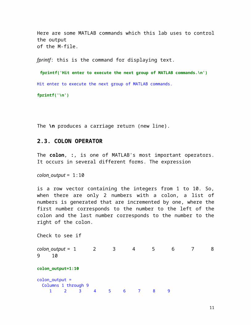
fprintf: this is the command for displaying text.

fprintf('Hit enter to execute the next group of MATLAB commands.\n')

Hit enter to execute the next group of MATLAB commands.

fprintf('\n')

The \n produces a carriage return (new line).

2.3. COLON OPERATOR

The colon, :, is one of MATLAB's most important operators. It occurs in several different forms. The expression

colon_output = 1:10

is a row vector containing the integers from 1 to 10. So, when there are only 2 numbers with a colon, a list of numbers is generated that are incremented by one, where the first number corresponds to the number to the left of the colon and the last number corresponds to the number to the right of the colon.

Check to see if

colon_output = 1 2 3 4 5 6 7 8 9 10

8

colon_output=1:10

colon_output = Columns 1 through 9 1 2 3 4 5 6 7 8 9 Column 10 10

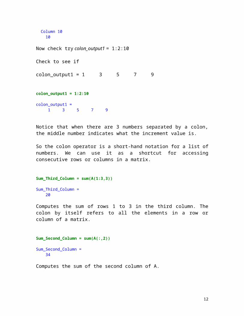
Now check try colon_output1 = 1:2:10 Check to see if

colon_output1 = 1 3 5 7 9

colon_output1 = 1:2:10

colon_output1 = 1 3 5 7 9

Notice that when there are 3 numbers separated by a colon, the middle number indicates what the increment value is.

So the colon operator is a short-hand notation for a list of numbers. We can use it as a shortcut for accessing consecutive rows or columns in a matrix.

Sum_Third_Column = sum(A(1:3,3))

Sum_Third_Column = 20

Computes the sum of rows 1 to 3 in the third column. The colon by itself refers to all the elements in a row or column of a matrix.

Sum_Second_Column = sum(A(:,2))

Sum_Second_Column = 34

Computes the sum of the second column of A.

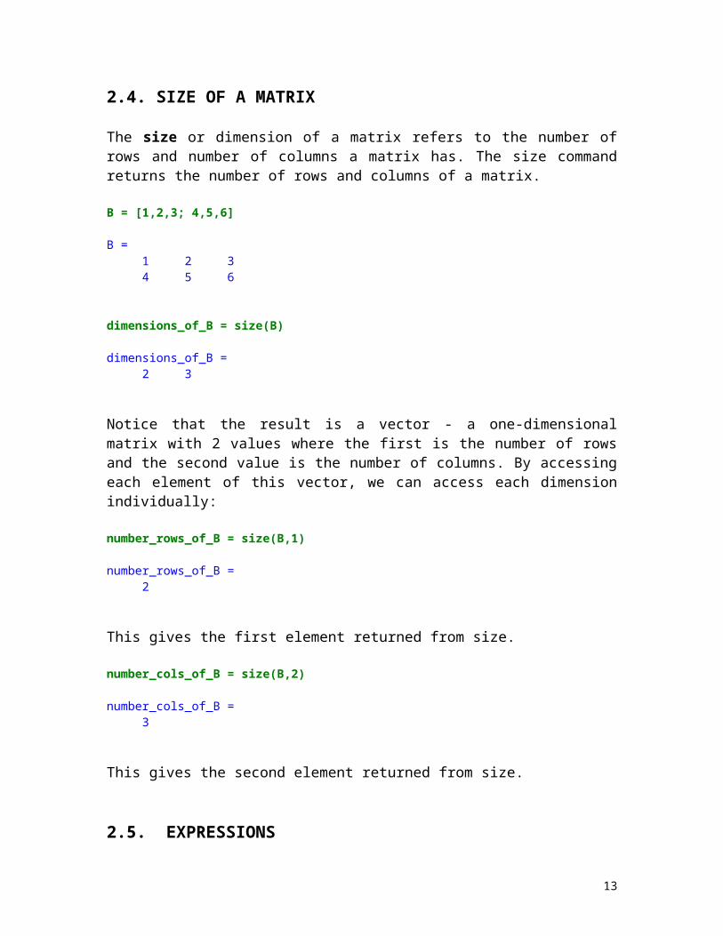
2.4. SIZE OF A MATRIX

The size or dimension of a matrix refers to the number of rows and number of columns a matrix has. The size command returns the number of rows and columns of a matrix.

9

B = [1,2,3; 4,5,6]

B = 1 2 3 4 5 6

dimensions_of_B = size(B)

dimensions_of_B = 2 3

Notice that the result is a vector - a one-dimensional matrix with 2 values where the first is the number of rows and the second value is the number of columns. By accessing each element of this vector, we can access each dimension individually:

number_rows_of_B = size(B,1)

number_rows_of_B = 2

This gives the first element returned from size.

number_cols_of_B = size(B,2)

number_cols_of_B = 3

This gives the second element returned from size.

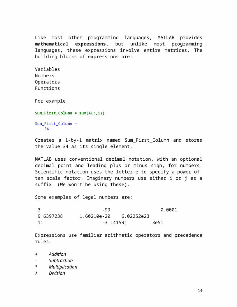
2.5. EXPRESSIONS

Like most other programming languages, MATLAB provides mathematical expressions, but unlike most programming languages, these expressions involve entire matrices. The building blocks of expressions are: VariablesNumbersOperatorsFunctions

For example

Sum_First_Column = sum(A(:,1))

10

Sum_First_Column = 34

Creates a 1-by-1 matrix named Sum_First_Column and stores the value 34 as its single element.

MATLAB uses conventional decimal notation, with an optional decimal point and leading plus or minus sign, for numbers. Scientific notation uses the letter e to specify a power-of-ten scale factor. Imaginary numbers use either i or j as a suffix. (We won't be using these).

Some examples of legal numbers are:

3 -99 0.0001 9.6397238 1.60210e-20 6.02252e23 1i -3.14159j 3e5i

Expressions use familiar arithmetic operators and precedence rules.

+ Addition- Subtraction* Multiplication/ Division^ Power' Complex conjugate transpose( ) Specify evaluation order

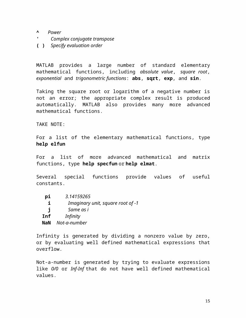
MATLAB provides a large number of standard elementary mathematical functions, including absolute value, square root, exponential and trigonometric functions: abs, sqrt, exp, and sin.

Taking the square root or logarithm of a negative number is not an error; the appropriate complex result is produced automatically. MATLAB also provides many more advanced mathematical functions.

TAKE NOTE:

For a list of the elementary mathematical functions, type help elfun

For a list of more advanced mathematical and matrix functions, type help specfun or help elmat.

Several special functions provide values of useful constants.

pi 3.14159265 i Imaginary unit, square root of -1

11

j Same as i Inf Infinity NaN Not-a-number

Infinity is generated by dividing a nonzero value by zero, or by evaluating well defined mathematical expressions that overflow.

Not-a-number is generated by trying to evaluate expressions like 0/0 or Inf-Inf that do not have well defined mathematical values.

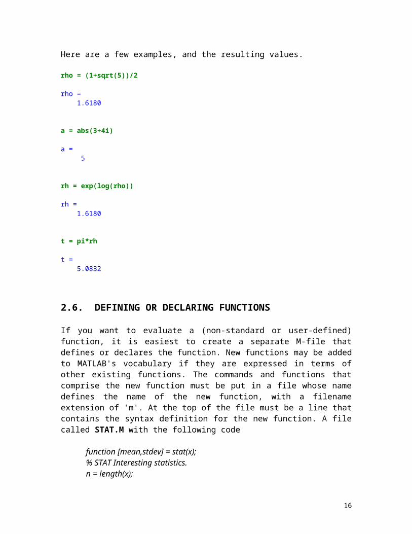
Here are a few examples, and the resulting values.

rho = (1+sqrt(5))/2

rho = 1.6180

a = abs(3+4i)

a = 5

rh = exp(log(rho))

rh = 1.6180

t = pi*rh

t = 5.0832

2.6. DEFINING OR DECLARING FUNCTIONS

If you want to evaluate a (non-standard or user-defined) function, it is easiest to create a separate M-file that defines or declares the function. New functions may be added to MATLAB's vocabulary if they are expressed in terms of other existing functions. The commands and functions that comprise the new function must be put in a file whose name defines the name of the new function, with a filename extension of 'm'. At the top of the file must be a line that contains the syntax definition for the new function. A file called STAT.M with the following code

function [mean,stdev] = stat(x); % STAT Interesting statistics. n = length(x);

12

mean = sum(x) / n; stdev = sqrt(sum((x - mean).^2)/n);

defines a new function called STAT that calculates the mean and standard deviation of a vector. The variables within the body of the function are all local variables (which means they only have values within that function).

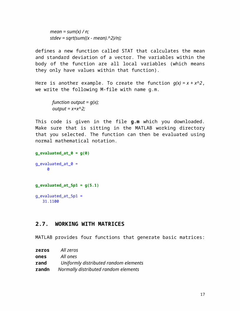
Here is another example. To create the function g(x) = x + x^2, we write the following M-file with name g.m.

function output = g(x);output = x+x^2;

This code is given in the file g.m which you downloaded. Make sure that is sitting in the MATLAB working directory that you selected. The function can then be evaluated using normal mathematical notation.

g_evaluated_at_0 = g(0)

g_evaluated_at_0 = 0

g_evaluated_at_5p1 = g(5.1)

g_evaluated_at_5p1 = 31.1100

2.7. WORKING WITH MATRICES MATLAB provides four functions that generate basic matrices:

zeros All zerosones All onesrand Uniformly distributed random elementsrandn Normally distributed random elements

Some examples:

Z = zeros(2,4)

Z = 0 0 0 0 0 0 0 0

13

This creates a 2 by 4 matrix of zeros.

F = 5*ones(3,3)

F = 5 5 5 5 5 5 5 5 5 This creates a 3 by 3 matrix, each element being a 5.

N = fix(10*rand(1,10))

N = Columns 1 through 9 9 2 6 4 8 7 4 0 8 Column 10 4

This creates a 1 by 10 matrix, each element being a random number generated by a uniform distribution from the interval [0,1]. The random number generated is multiplied by 10 and only the (rounded) integer part is retained.

R = randn(4,4)

R = -0.4326 -1.1465 0.3273 -0.5883 -1.6656 1.1909 0.1746 2.1832 0.1253 1.1892 -0.1867 -0.1364 0.2877 -0.0376 0.7258 0.1139

This creates a 4 by 4 matrix, each element being a random number generated by a normal distribution.

2.8. MATRICES AND ARRAYS

Linear Algebra and Arrays

Informally, the terms matrix and array are often used interchangeably. More precisely, a matrix is a two-dimensional numeric array that represents a linear transformation. The mathematical operations defined on matrices are the subject of linear algebra.

When they are taken away from the world of linear algebra, matrices become two dimensional numeric arrays. Arithmetic operations on arrays are done element-by-element. This means that addition and subtraction are the same for arrays and matrices, but that multiplicative operations are different.

14

MATLAB uses a dot, or decimal point, as part of the notation for multiplicative array operations. The list of operators includes:

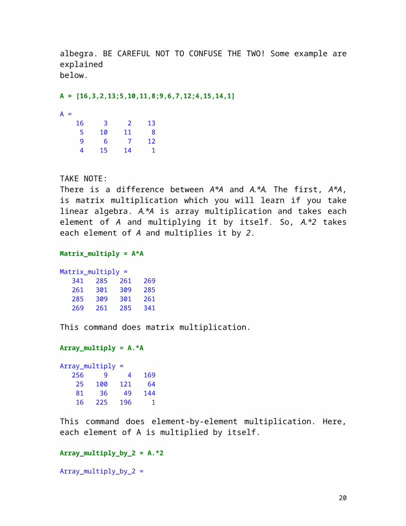
+ Addition- Subtraction.* Element-by-element multiplication./ Element-by-element division.^ Element-by-element power.' Unconjugated array transpose. The transpose operator swaps rows and columns and so all rows become columns and all columns become rows. !!! IMPORTANT !!!The operations listed above are for array or element-by-element operations, which is what we will be using in this course. There are similar operations used for matrix operations, including *, / , ^ , ' which are used in linear albegra. BE CAREFUL NOT TO CONFUSE THE TWO! Some example are explainedbelow. A = [16,3,2,13;5,10,11,8;9,6,7,12;4,15,14,1]

A = 16 3 2 13 5 10 11 8 9 6 7 12 4 15 14 1

TAKE NOTE:There is a difference between A*A and A.*A. The first, A*A, is matrix multiplication which you will learn if you take linear algebra. A.*A is array multiplication and takes each element of A and multiplying it by itself. So, A.*2 takes each element of A and multiplies it by 2.

Matrix_multiply = A*A

Matrix_multiply = 341 285 261 269 261 301 309 285 285 309 301 261 269 261 285 341

This command does matrix multiplication.

Array_multiply = A.*A

Array_multiply = 256 9 4 169 25 100 121 64 81 36 49 144 16 225 196 1

15

This command does element-by-element multiplication. Here, each element of A is multiplied by itself.

Array_multiply_by_2 = A.*2

Array_multiply_by_2 = 32 6 4 26 10 20 22 16 18 12 14 24 8 30 28 2

This command multiplies each element of A by 2.

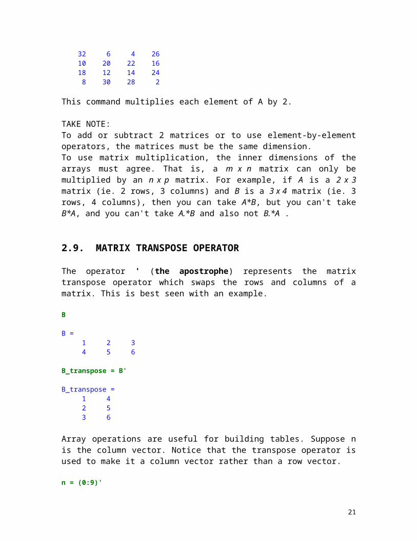
TAKE NOTE:To add or subtract 2 matrices or to use element-by-element operators, the matrices must be the same dimension. To use matrix multiplication, the inner dimensions of the arrays must agree. That is, a m x n matrix can only be multiplied by an n x p matrix. For example, if A is a 2 x 3 matrix (ie. 2 rows, 3 columns) and B is a 3 x 4 matrix (ie. 3 rows, 4 columns), then you can take A*B, but you can't take B*A, and you can't take A.*B and also not B.*A .

2.9. MATRIX TRANSPOSE OPERATOR

The operator ' (the apostrophe) represents the matrix transpose operator which swaps the rows and columns of a matrix. This is best seen with an example.

B

B = 1 2 3 4 5 6

B_transpose = B'

B_transpose = 1 4 2 5 3 6

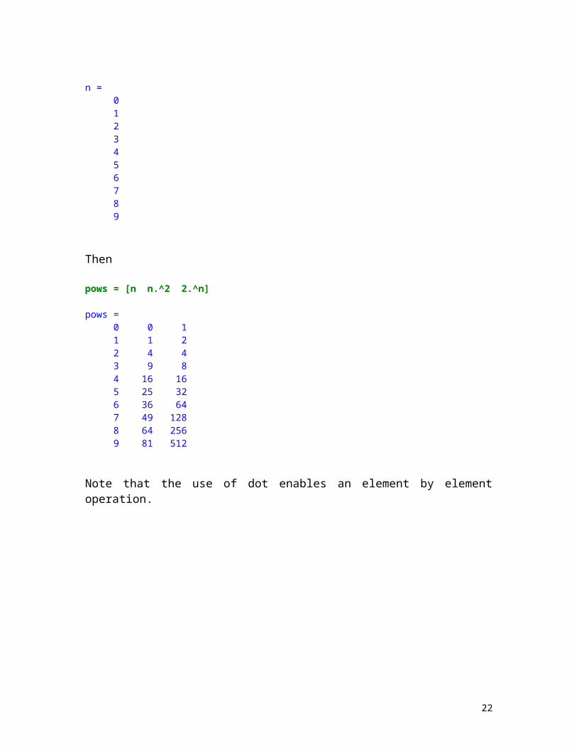
Array operations are useful for building tables. Suppose n is the column vector. Notice that the transpose operator is used to make it a column vector rather than a row vector.

n = (0:9)'

n = 0 1 2

16

3 4 5 6 7 8 9

Then

pows = [n n.^2 2.^n]

pows = 0 0 1 1 1 2 2 4 4 3 9 8 4 16 16 5 25 32 6 36 64 7 49 128 8 64 256 9 81 512

Note that the use of dot enables an element by element operation.

17

3. GRAPHICS3.1. PLOTTING GRAPHS

There are 2 methods for plotting graphs in MATLAB and 2 ways to display your graph output.

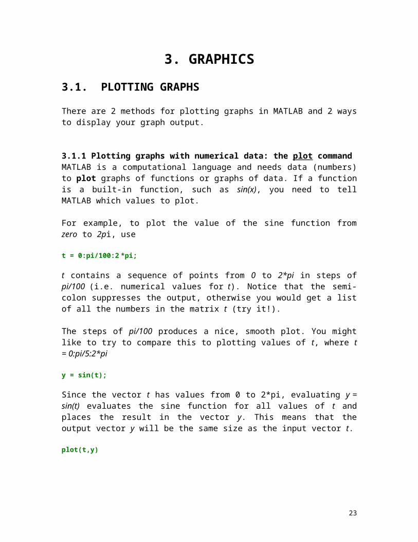
3.1.1 Plotting graphs with numerical data: the plot commandMATLAB is a computational language and needs data (numbers) to plot graphs of functions or graphs of data. If a function is a built-in function, such as sin(x), you need to tell MATLAB which values to plot. For example, to plot the value of the sine function from zero to 2pi, use

t = 0:pi/100:2 *pi;

t contains a sequence of points from 0 to 2*pi in steps of pi/100 (i.e. numerical values for t). Notice that the semi-colon suppresses the output, otherwise you would get a list of all the numbers in the matrix t (try it!).

The steps of pi/100 produces a nice, smooth plot. You might like to try to compare this to plotting values of t, where t = 0:pi/5:2*pi

y = sin(t);

Since the vector t has values from 0 to 2*pi, evaluating y = sin(t) evaluates the sine function for all values of t and places the result in the vector y. This means that the output vector y will be the same size as the input vector t.

plot(t,y)

18

0 1 2 3 4 5 6 7-1

-0.8

-0.6

-0.4

-0.2

0

0.2

0.4

0.6

0.8

1

This creates a plot of y versus t and embeds the result in your Word document. Plotting data numerically is useful when you don't necessarily have a function to describe or model the data.

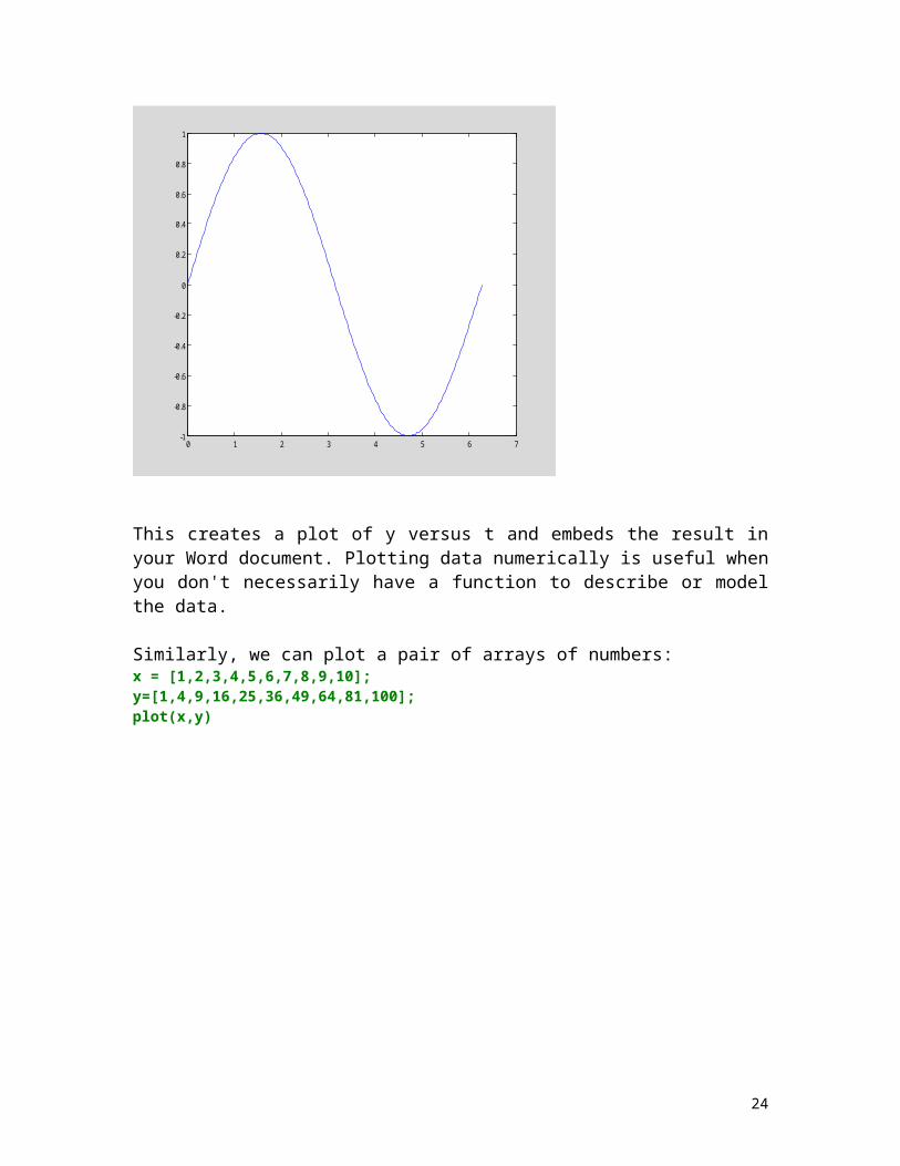
Similarly, we can plot a pair of arrays of numbers:x = [1,2,3,4,5,6,7,8,9,10];y=[1,4,9,16,25,36,49,64,81,100];plot(x,y)

1 2 3 4 5 6 7 8 9 100

10

20

30

40

50

60

70

80

90

100

19

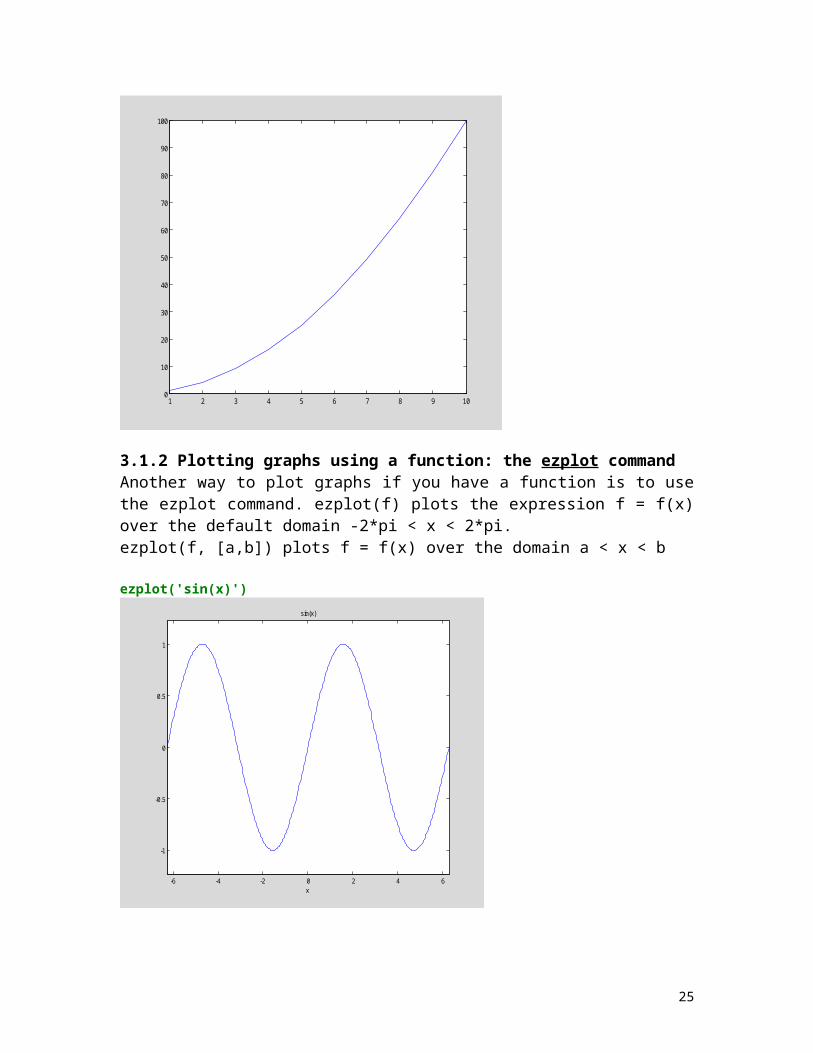
3.1.2 Plotting graphs using a function: the ezplot commandAnother way to plot graphs if you have a function is to use the ezplot command. ezplot(f) plots the expression f = f(x) over the default domain -2*pi < x < 2*pi.ezplot(f, [a,b]) plots f = f(x) over the domain a < x < b

ezplot('sin(x)')

-6 -4 -2 0 2 4 6

-1

-0.5

0

0.5

1

x

sin(x)

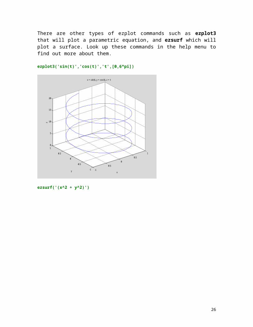
There are other types of ezplot commands such as ezplot3 that will plot a parametric equation, and ezsurf which will plot a surface. Look up these commands in the help menu to find out more about them.

ezplot3('sin(t)','cos(t)','t',[0,6*pi])

20

-1

-0.5

0

0.5

1

-1

-0.5

0

0.5

10

5

10

15

20

x

x = sin(t), y = cos(t), z = t

y

z

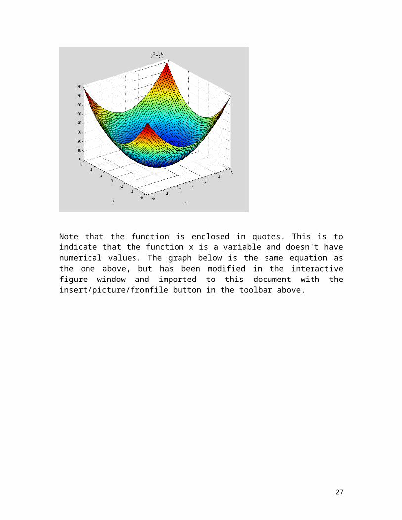
ezsurf('(x^2 + y^2)')

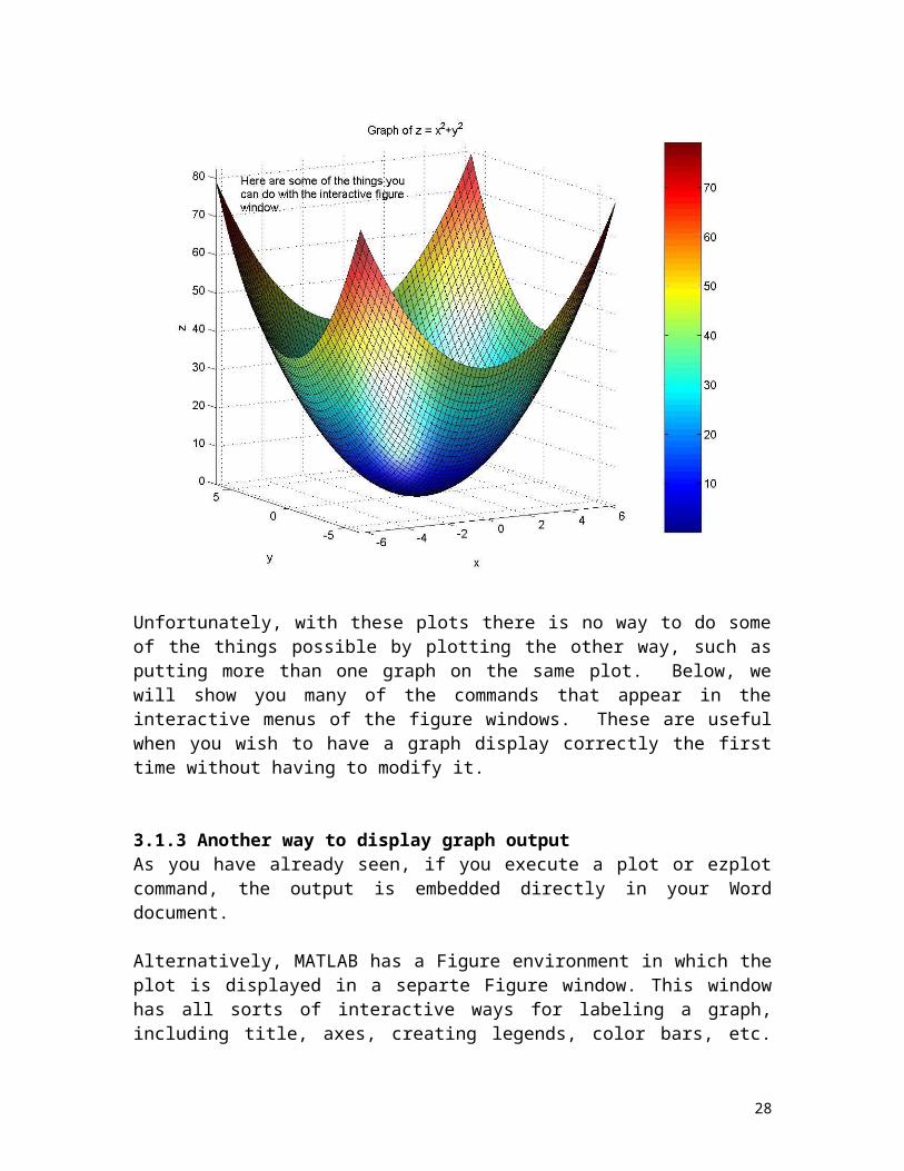
Note that the function is enclosed in quotes. This is to indicate that the function x is a variable and doesn't have numerical values. The graph below is the same equation as the one above, but has been modified in the interactive figure window and imported to this document with the insert/picture/fromfile button in the toolbar above.

21

Unfortunately, with these plots there is no way to do some of the things possible by plotting the other way, such as putting more than one graph on the same plot. Below, we will show you many of the commands that appear in the interactive menus of the figure windows. These are useful when you wish to have a graph display correctly the first time without having to modify it.

3.1.3 Another way to display graph outputAs you have already seen, if you execute a plot or ezplot command, the output is embedded directly in your Word document.

Alternatively, MATLAB has a Figure environment in which the plot is displayed in a separte Figure window. This window has all sorts of interactive ways for labeling a graph, including title, axes, creating legends, color bars, etc. Make sure you try out some of the options under the Insert and Tools menus. These will be extremely useful items to use throughout this course.

To use this feature, you will be typing your commands at the MATLAB prompt (in the MATLAB program). First you create a figure window and then plot your graph. Type the following commands at the MATLAB prompt.

t = 0:pi/100:2*pi;

22

y = sin(t);figure(1); plot(t,y)

If you use the Figure window, you can save your plots using the File menu from the Figure Window tool bar. File->Save save the plot as a .fig file which can be read back into MATLAB. Alternatively, File->Export allows you to save the plot in a graphics format, such a jpg, tiff or eps. You can select the format by selecting the appropriate format in the "Save as Type" scroll bar in the export window.

You will likely want to export your plots as a jpg format so you can then import into them a Word document (using Insert->Picture->From File) when writing up your lab report.

3.2. PLOTTING MULTPLE GRAPHS ON THE SAME PLOT

Next, we plot three related functions of t, with each curve in a separate distinguishing color.

MATLAB gives a different color to each curve automatically. You will see how to change colors later.

y2 = sin(t-.25); y3 = sin(t-.5); plot(t,y,t,y2,t,y3)

0 1 2 3 4 5 6 7-1

-0.8

-0.6

-0.4

-0.2

0

0.2

0.4

0.6

0.8

1

23

First the x values, and then the y values are listed for each graph

If you were to type this commands in MATLAB and want them to appear in a new figure window, then you would type the command figure(2) before doing the plot command to create a new (second figure window). Otherwise the plot would appear in the previous window.

3.3. PLOTTING OPTIONS: color, linestyle, markers, axes labels, legend, titles

You can and should enhance your graphs with axes labels, titles and color and legends if appropriate. You can either use the following Matlab commands to enhance your graphs. These commands work with graphs you are going to embed in your document or graphs in the Figure environment. However, it is usually much easier to label your graphs interactively using the Figure window tool bar by using the Insert and Tools menus.

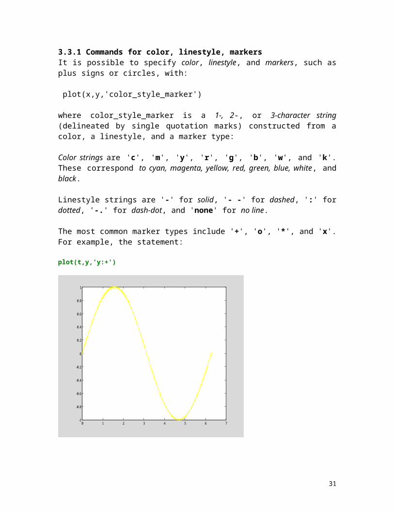
3.3.1 Commands for color, linestyle, markersIt is possible to specify color, linestyle, and markers, such as plus signs or circles, with:

plot(x,y,'color_style_marker')

where color_style_marker is a 1-, 2-, or 3-character string (delineated by single quotation marks) constructed from a color, a linestyle, and a marker type:

Color strings are 'c', 'm', 'y', 'r', 'g', 'b', 'w', and 'k'. These correspond to cyan, magenta, yellow, red, green, blue, white, and black.

Linestyle strings are '-' for solid, '- -' for dashed, ':' for dotted, '-.' for dash-dot, and 'none' for no line.

The most common marker types include '+', 'o', '*', and 'x'. For example, the statement:

plot(t,y,'y:+')

24

0 1 2 3 4 5 6 7-1

-0.8

-0.6

-0.4

-0.2

0

0.2

0.4

0.6

0.8

1

plots a yellow dotted line and places plus sign markers at each data point.

If you specify a marker type but not a linestyle, MATLAB draws only the marker. For example, plot(t,y,'o') would plot only points.

3.3.2. Commands for axis labels, legends, titlesMATLAB commands can be used to label your graphs. As described above, axis labels, legends and titles can be placed on a graph using the Insert and Tools menus from the Figure Window tool bar. Usually it is much easier to use the tool bar.

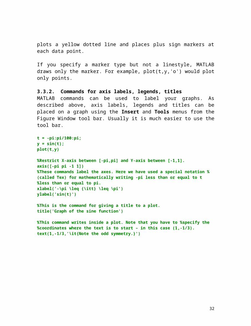
t = -pi:pi/100:pi; y = sin(t); plot(t,y)

%Restrict X-axis between [-pi,pi] and Y-axis between [-1,1]. axis([-pi pi -1 1]) %These commands label the axes. Here we have used a special notation %(called Tex) for mathematically writing -pi less than or equal to t %less than or equal to pi. xlabel('-\pi \leq {\itt} \leq \pi') ylabel('sin(t)')

%This is the command for giving a title to a plot. title('Graph of the sine function')

25

%This command writes inside a plot. Note that you have to %specify the %coordinates where the text is to start – in this case (1,-1/3). text(1,-1/3,'\it{Note the odd symmetry.}')

-3 -2 -1 0 1 2 3-1

-0.8

-0.6

-0.4

-0.2

0

0.2

0.4

0.6

0.8

1

- t

sin(

t)

Graph of the sine function

Note the odd symmetry.

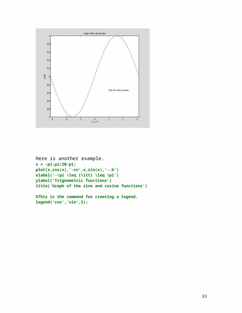
Here is another example.x = -pi:pi/20:pi; plot(x,cos(x),'-ro',x,sin(x),'-.b') xlabel('-\pi \leq {\itt} \leq \pi') ylabel('Trignometric functions') title('Graph of the sine and cosine functions')

%This is the command for creating a legend. legend('cos','sin',2);

26

-4 -3 -2 -1 0 1 2 3 4-1

-0.8

-0.6

-0.4

-0.2

0

0.2

0.4

0.6

0.8

1

- t

Trig

nom

etric

func

tions

Graph of the sine and cosine functions

cossin

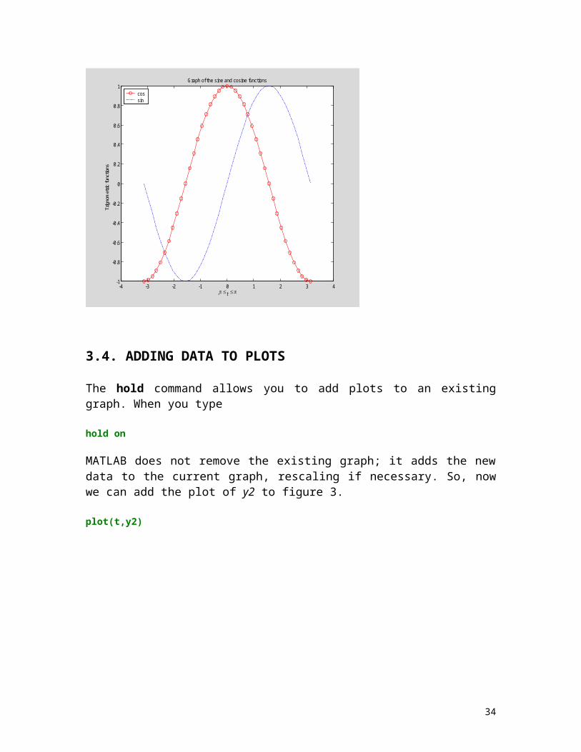
3.4. ADDING DATA TO PLOTS

The hold command allows you to add plots to an existing graph. When you type

hold on

MATLAB does not remove the existing graph; it adds the new data to the current graph, rescaling if necessary. So, now we can add the plot of y2 to figure 3.

plot(t,y2)

27

-4 -3 -2 -1 0 1 2 3 4-1

-0.8

-0.6

-0.4

-0.2

0

0.2

0.4

0.6

0.8

1

- t

Trig

nom

etric

func

tions

Graph of the sine and cosine functions

cossin

hold off

(Remember to turn the hold off!)

3.5. 3D PLOTS

One of the nice feature of MATLAB is that you can created 3D graphs and interact with them directly by rotating the graph to see it from different view points. In order to create a graph of surface in 3-space, t is necessary to evaluate the function on a regular rectangular grid. This can be done using the meshgrid command. First create 1 D vector describing the grids in the x- and y-directions:

x = (0:2*pi/20:2*pi)'; y = (0:4*pi/40:4*pi)';

Next, spread these grids into two dimensions using meshgrid:

[X,Y] = meshgrid(x,y);

The effect of meshgrid is to create a vector X wih the x-grid aking each row, and a vector Y with the y-grid along each column. Then using vectorized functions and/or operators, it is easy to evaluate a function z=f(x,y) of two variables on the rectangular grid:

28

z = cos(X).*cos(2*Y);

Having create the matrix containing the samples of the function, the surface can be graphed using either the mesh or the surf commands:

mesh(x,y,z)

surf(x,y,z)

29

In addition, a contour plot can be created

contour (x,y,z)

0 1 2 3 4 5 60

2

4

6

8

10

12

If you execute these commands within MATLAB to use the Figure environment, you can rotate these graphs interactively by using the circular dashed arrow icon. Try it!

3.6. SUBPLOT FUNCTION

The subplot function allows you to display multiple plots in the same window or print them on the same piece of paper. Typing subplot(m,n,p) breaks the figure window into an m-by-n matrix of small subplots and selects the pth subplot for the current plot.

The plots are numbered along first the top row of the figure window, then the second row, and so on. For example, to plot data in four different subregions of the figure window,

figure(4);t = 0:pi/10:2*pi;[X,Y,Z] = cylinder(4*cos(t)); subplot(2,2,1); mesh(X) subplot(2,2,2); mesh(Y)subplot(2,2,3); mesh(Z)subplot(2,2,4); mesh(X,Y,Z)

30

The coordinates of 4*cos(t) are stored in X,Y and Z.

Use the figure command to make sure all subsequent plots are placed in a new figure rather than in the subplot.

31

4. ANIMATIONMATLAB provides several ways of generating moving, animated, graphics.

Using the EraseMode property is appropriate for long sequences of simple plots where the change from frame to frame is minimal. Here is an example showing simulated Brownian motion. You must execute these commands within MATLAB.

First we are going to specify a number of points and then a temperature or velocity. The best values for these two parameters depend upon the speed of your particular computer. Execute the following commands in MATLAB (ie. copy and paste from here to MATLAB) to see the animation.

% Animation of Brownian Motion

% Specify a number of pointsn = 20;

% Specify a temperature or velocitys = .02;

% Generate n random points with (x,y) coordinates between -1/2 and +1/2 x = rand(n,1)-0.5; y = rand(n,1)-0.5;

% Plot the points in a square with sides from –1 to +1h = plot(x,y,'.'); axis([-1 1 -1 1]) xlabel('X-Axis') ylabel('Y-Axis') title('Simulation of a Brownian Motion')

% Make the scale of the x-axis and the y-axis equal axis square % Command to suppress the grid (see what happens if you say grid % on)grid off

% Don't worry about this command for nowset(h,'EraseMode','xor','MarkerSize',18)

% This is where the anmiation starts

temp = 1; fprintf('Wait until the animation is over.\n\n')while temp < 5000 drawnow x = x + s*randn(n,1); y = y + s*randn(n,1); set(h,'XData',x,'YData',y) temp = temp+ 1; end

32

Don't worry about the command set(h,'EraseMode','xor','MarkerSize',18). If you are interested, it saves the handle for the vector of points and set its EraseMode to xor. This tells the MATLAB graphics system not to redraw the entire plot when the coordinates of one point are changed, but to restore the background color in the vicinity of the point using an "exclusive or" operation.

So what is happening? The statements between the while and the end create a loop of 5000 iterations (for temp between 1 and 4999). Each time through the loop, a small amount of normally distributed random noise is added to the x and y coordinates of the points. Then, instead of creating an entirely new plot, simply change the Xdata and YData properties of the original plot to replot the data.

33

5. LAB REPORTSYour lab report is to be a typed document that contains answers to the lab questions.

It is probably easiest to create this report using a MATLAB Notebook which contains your MATLAB commands and results. Make sure you also give a written description to any lab questions and import any graphical results.

If you created any M-files that contain MATLAB commands used to generate your results, you should also include this with your report. Make sure your report describes or explains what the M-file is. Also make sure your M-file has comments in it explaining what it does.

When you are finished your assignement, you should be able to evaluate the entire Notebook (Notebook->Evaluate M-book) and you entire assisngment should execute correctly.

6. ADDITIONAL HELPThere is lots of help available through the MATLAB menus. Additionally you can type help at the MATLAB prompt, or help command-name to get help on a specific command. For example, help plot

For a list of the elementary mathematical functions, type: help elfunFor a list of specialized math functions, type: help specfunFor a list of matrix manipulation functions, type: help elmat

To see some more demos on some of the MATLAB features, type: demo

There are lots of internet resources available too. This concludes this introductory lab module.

34