the mathematics of modern growth theory - stephen...

The Mathematics of Modern Growth Theory

Stephen Kinsella

Department of Economics,Kemmy Business School,University of Limerick, Limerick, Ireland

[email protected]

www.stephenkinsella.net

Abstract. These notes provide an overview of modern growth theory as it is taught in graduate schoolsaround the world. I provide a Mathematica implementation of the workhorse models of modern growththeory as a pedagogical aid. Further work will focus on transforming these Mathematica 5.0implementations into Mathematica 6.0 Demonstrations.

Initialisations (Press ˜÷Û)

In[77]:= Off@General::spell, General::spell1DOff@InverseFunction::ifunDOff@Solve::ifunD

Introduction: defining terms

Theories of economic growth are central to most mainstream textbooks in macroeconomics. At one time or another,

they have occupied the greatest minds in the discipline. The stakes being played for in the game to get economic growth

right are enormous. "Once you start thinking about it, its very hard to think about anything else", to paraphrase Nobel

Laureate Robert Lucas. While Lucas was wrong about a great many things, he was correct on this point. If real Gross

Domestic Product (GDP) is a measure of the output of an open economy at a certain point in time, then economic

growth can be defined as the year on year increase of GDP. Through compounding, a year on year increase in GDP of

5% corresponds to a doubling of living standards every 25 years.

DEFINITION (GDP) Gross Domestic Product !is the total market value of the goods and services produced by a

nation's economy during a specific period of time.

Some qualifications are in order though. First, the GDP we will talk about is real GDP|||it is GDP corrected for the

changes in prices over the time period we are measuring. Second, the GDP we will measure is gross, in that this

measure includes the replacement of worn out and obsolete equipment and structures in the economy, as well as

completely new (or autonomous) investment. We don't use net measures because the information needed to create them

is unreliable. Third, we will normally talk about GDP per worker (sometimes called per capita), which is real GDP

divided by the number of workers in the economy. This is the most commonly used index of development or growth in

the economy, and is part of the Lingua Franca of modern economics, so you'd better know something about it.

Why should a student in Ireland care about economic growth? Well, the fact that you are taking this course is proof-

positive that economic growth can affect the wellbeing of a population. Irish economic growth over the past 15 years

has been nothing short of miraculous. For details on the Irish economic experience, consult O'Hagan and Newman,

(2005), or Honohan, (2002). If you are reading this, you are likely to be twice as well off in terms of living standards

than your parents. So, if your parents could afford one annual holiday, you can afford two, on average.

"Wellbeing" can be defined in many ways, and GDP per worker does have its critics, for example Joseph Stiglitz

(http://www.argmax.com/mt_blog/archive/000671.php). Stiglitz's main arguments are GDP does not take account of (1)

degradation of the environment and use of natural resources, (2) depreciation, and (3) payments to foreigners, and he is

not alone.

So GDP per worker is far from a perfect measure, but it is the standard measure of economic wellbeing, and so we must

use it. The table below shows an index of GDP per capita for each of the EU 15 countries and some composites.

Printed by Mathematica for Students

So GDP per worker is far from a perfect measure, but it is the standard measure of economic wellbeing, and so we must

use it. The table below shows an index of GDP per capita for each of the EU 15 countries and some composites.

Table 1. GDP per capita in Purchasing Power Standards, 2001-2003

EU 25=100

Country 2001 2002 20032003

Luxembourg 213.3 212.6 214.7

Ireland (GDP) 129.5 132.6 132.5

Denmark5 126.3 122.5 122.6

Austria 124.4 122.7 122.2

Netherlands 124.2 122.0 121.0

United King5 115.1 117.8 118.5

Belgium 117.3 116.7 117.8

Sweden5 116.4 114.8 115.2

Finland 114.1 113.7 113.7

Ireland (GNI) 109.8 109.7 111.0

France 114.8 112.9 111.0

Germany 110.1 108.7 108.1

Italy5 109.6 109.0 106.9

EU 25 100.0 100.0 100.0

Spain5 92.3 94.6 97.8

Cyprus 88.8 82.9 81.3

Greece 73.8 77.7 80.9

Slovenia 74.8 75.3 76.8

Portugal 77.2 76.7 74.7

Malta 74.6 73.8 73.8

Czech Republ 66.1 67.6 68.8

Hungary 56.4 58.6 60.5

Slovakia 48.9 51.3 52.1

Estonia 44.8 46.6 48.5

Poland 45.9 45.6 46.0

Lithuania 40.8 42.4 45.8

Latvia 37.4 38.9 41.0

Norway5 158.2 149.5 147.7

Iceland5 125.3 119.8 118.7

Bulgaria5 28.6 28.8 29.7

Romania 26.7 28.6 29.6

Source: Eurostat and Irish National Accounts, see http://www.cso.ie/releasespublications/measuringirelandsprogress2004.htm for

more details.

And the figure below shows Irish real GDP per capita. This is not a growth rate, however. You're going to figure that

out for yourselves in exercise 1.

gdpdata = Import@"irlgdp.csv", "csv"D;ListPlot@gdpdata, AxesLabel Ø 8"Year", "Real GDP Per Capita"<D

1960 1970 1980 1990 2000Year

5000

10000

15000

20000

25000

30000

Real GDP Per Capita

Irish Real GDP per Capita, 1950-2005. Source: Penn World Tables v. 6.2, CSO.ie, and author's calculations. Penn Data available here, CSO data availabe here.

A Word about Growth Rates

We will be talking about rates of growth of measured economic quantities like GDP and the capital stock, so its

important you understand what I mean by this term. The rate of growth of GDP is expressed as an index normally, that

is, we talk about the difference between the calculated GDP of two years, divided by the 'base' or reference year, and

normally expressed as a percentage. If we take two years, 2004 and 2005, and 2004 is the base year, then g, the growth

rate of GDP, is given by equation 1 below.

2 growththeorymacronotes_v3.nb


(1)g =GDP2005 - GDP2004

GDP2004.

ü Exercise 1

Your first exercise is to calculate the growth rates in the excel sheet (NUIG_MACRO_EX_1.nb) downloadable from

http://www.stephenkinsella.net. Answer the following questions.

1. Calculate the rate of growth of the Irish economy, using 1995 as the base year.

2. Graph the change in growth rates against time from 1995 -2005 with time on the x-axis.

3. Is growth accelerating? Based on the evidence you have just created and nothing else, what are your predictions for

growth 3 years into the future, from 2005 to 2008?

Mathematical Terms

When I say these words in the lectures, these are the meanings I'm ascribing to them. I won't dwell on these too long,

but you need to know them to do well in the course. You'll see references at the end of each definition: in the online

version of this lecture note, you can investigate each property further. There are lots of links here to explore; just use the

ones you need to get up to speed quickly.

DEFINITION (Vector) Vector means several things to us in this course. A quantity, such as velocity,completely

specified by a magnitude and a direction. 2. A one-dimensional array. 3. An element of a vector space. (ref here)

DEFINITION (Matrix) A matrix (plural matrices) is a rectangular table of numbers or, more generally, a table

consisting of abstract quantities that can be added and multiplied. Matrices are used to describe linear equations, keep

track of the coefficients of linear transformations and to record data that depend on two parameters (ref here).

DEFINITION (Space) A topological space is a set X together with a collection T of subsets of X satisfying the

following axioms:

1. The empty set and X are in T.

2. The union of any collection of sets in T is also in T.

3. The intersection of any pair of sets in T is also in T.

The collection T is a topology on X, and the elements of X are called points. The sets in T are the open sets, and their

complements in X are the closed sets. The requirement that the union of any collection of open sets be open is more

stringent than simply requiring that all pairwise unions be open, as the former includes unions of infinite collections of

sets. It follows that a closed set must satisfy the following:

1. The empty set and X are closed (as well as being open).

2. The intersection of any collection of closed sets is also closed.

3. The union of any pair of closed sets is also closed,

By induction, the intersection of any finite collection of open sets is open. (ref here)

DEFINITION (Metric Space) A set where a notion of distance between elements of the set is defined. The metric space

which most closely corresponds to our intuitive understanding of space is the 3-dimensional Euclidean space. A metric

space induces topological properties like open and closed sets which leads to the study of even more abstract topological

spaces (ref here).

DEFINITION (Open Sets) In topology and related fields of mathematics, a set U is called open if, intuitively speaking,

you can wiggle or change any point x in U by a small amount in any direction and still be inside U. In other words, if x

is surrounded only by elements of U; it can't be on the edge of U.

As a typical example, consider the open interval (0,1) consisting of all real numbers x with 0 < x < 1. Here, the topology

is the usual topology on the real line. If you wiggle such an x a little bit (but not too much), then the wiggled version

will still be a number between 0 and 1. Therefore, the interval (0,1) is open. However, the interval (0,1] consisting of all

numbers x with 0 < x § 1 is not open; if you take x = 1 and move even the tiniest bit in the positive direction, you will

be outside of (0,1]. (ref here)

DEFINITION (Closed Sets) A closed set contains its own boundary. In other words, if you are "outside" a closed set

and you "wiggle" a little bit, you will stay outside the set.(ref here)

Any intersection of arbitrarily many closed sets is closed, and any union of finitely many closed sets is closed. In

particular, the empty set and the whole space are closed. In fact, given a set X and a collection F of subsets of X that has

these properties, then F will be the collection of closed sets for a unique topology on X. The intersection property also

allows one to define the closure of a set A in a space X, which is defined as the smallest closed subset of X that is a

superset of A. Specifically, the closure of A can be constructed as the intersection of all of these closed supersets.

growththeorymacronotes_v3.nb 3


DEFINITION (Closed Sets) A closed set contains its own boundary. In other words, if you are "outside" a closed set

and you "wiggle" a little bit, you will stay outside the set.(ref here)

Any intersection of arbitrarily many closed sets is closed, and any union of finitely many closed sets is closed. In

particular, the empty set and the whole space are closed. In fact, given a set X and a collection F of subsets of X that has

these properties, then F will be the collection of closed sets for a unique topology on X. The intersection property also

allows one to define the closure of a set A in a space X, which is defined as the smallest closed subset of X that is a

superset of A. Specifically, the closure of A can be constructed as the intersection of all of these closed supersets.

DEFINITION (Bounded Sets in Metric Spaces) A set S of real numbers is called bounded above if there is a real

number k such that k ¥ s for all s in S. The number k is called an upper bound of S. The terms bounded below and lower

bound are similarly defined. A subset S of a metric space (M, d) is bounded if it is contained in a ball of finite radius, i.e.

if there exists x in M and r > 0 such that for all s in S, we have d(x, s) < r. M is a bounded metric space (or d is a

bounded metric) if M is bounded as a subset of itself. Properties which are similar to boundedness but stronger, that is

they imply boundedness, are total boundedness and compactness.

A set S is bounded if it is bounded both above and below. Therefore, a set of real numbers is bounded if it is contained

in a finite interval (ref here).

DEFINITION (Banach Fixed Point/Contraction-Mapping Theorem) The Banach fixed point theorem (also known as

the contraction mapping theorem or contraction mapping principle) is an important tool in the theory of metric spaces; it

guarantees the existence and uniqueness of fixed points of certain self maps of metric spaces, and provides a semi-

constructive method to find those fixed points. The theorem is named after Stefan Banach (1892-1945), and was first

stated by Banach in 1922. ( ref to Full version of proof)

Calculus and Growth Rates

Obviously we will want to use calculus to derive analytical results about models of growth. Calculus should have you

thinking about derivatives. One of the assumptions we need to take a derivative of a quantity with respect to another is

very small (or infinitesimal) changes. The assumption is made here (and everywhere) that we can do this. So, you will

see me trying to find out if the capital stock, K, is growing over time, t. We will need to find out if !K/!t (or K°

)> 0. The

way we do this trick of moving from a yearly data point to an infinitesimally small one is by taking a limit, or imagining

a decrease in the size of the gap between the two observations (let's let this gap be given by D. Then equation 2 gives us

(2)LimDtØ0

Kt - Kt-Dt

Dt=

!K

! t= K

°.

Having got our instantaneous change, we need to look how that changed relative to what was already there, so our

growth rate would be given by K°

/K. We will be using this formalism a lot, so get used to it. We will also be using lots of

logarithm transformations, which I detail in the Lagrangian section below. Also, Jones (1998, pp. 167-169) has a good

exposition of these rules.

Having defined my terms somewhat, let me take you through three mathematical tools you will need to understand

before we touch on models of growth theory in Romer. First, we'll look at differential equations, then linear

programming, then dynamic programming.

ü Exercise 2

If Y = KHaL ALH1-aL, where Y is output, K is capital employed and AL is technology -augmented (Harrod-neutral)

labour, with a being the share of capital employed in producing output, and assuming constant returns to scale, use this

equation to find

1. dY

dKand

d2 Y

dK2

;

2. dY

dLand

d2 Y

dL2.

3. Assume these functions are time dependent, so Y@tD = K@tDHaL AL@tDH1-aL. What is dY/dt? Is is greater than 0?



Solving Differential Equations for dummies

Now for a little unpleasantness. Dynamical systems use terms like stability in a very specific way, so to get through the

solution algorithm, we need to define more terms, and very precisely this time.

We want to investigate and visualize the dynamics of the first-order difference equation

(3)xn+1 = f HxnLwhere f is given function. We will often refer to such a difference equation as a map f or one-dimensional dynamical

system.

DEFINITION (Orbit). A positive orbit of x0 is the set of points {x0, f(x0), f(f(x0)), . . .}, and is denoted by O(x0).

DEFINITION (Equilibrium (Fixed) Point). The point q is called an equilibrium (fixed) point for f if f(q) = q.

DEFINITION (Periodic Point). A point p is called a periodic point of minimal period n if

fn HpL = f(...f(p)...) = p and n is the least such positive integer. The set of all iterates of a periodic point is called a

periodic orbit. In other words, a periodic point p of minimal period n is a fixed point of the map fn HxL = f(...f(x)...).

The geometric method for visualization of the solutions of our one-dimensional difference equation (3) is called the

stair-step diagram. You proceed by plotting the pairs Hxn, xn+1) , n = 0,1, ... in the standard rectangular coordinate

system and connecting the pair of points Hxn, xn+1) and Hxn+1, xn+1) and Hxn+1, xn+1) and Hxn+1, xn+2) with the

segments of the straight line, just like you did for your Junior Cert when drawing graphs. The line segments mentioned

above build an impression of stairs. Also, it is important to observe that the fixed points of Eq(3) are the points of

intersection of the graph of f with the diagonal y = x.

In this economics, we're especially interested in stability of fixed points. It has been shown that, under certain

conditions, the stability type of the fixed point q of Eq(3) is the same as the stability type of the fixed point of the

corresponding linearized equation:

(4)yn+1 = f ' HqL yn

The stability of Eq(4) is evident from the stair-case diagrams. This suggests the following linearized stability theorem

about a fixed point.

THEOREM ( Linearized Stability ). Let f be continuously differentiable function defined on !. A fixed point q of f is

asymptotically stable if | f ' (q) | <1, and it is unstable if | f ' (q) | >1.

We introduce the following notion for fixed points of Eq(1):

DEFINITION (Hyperbolic Fixed Point). A fixed point q of Eq(1) is said to be hyperbolic if | f ' (q) | is not equal 1.

From linearized stability theorem, if a fixed point q of Eq(1) is hyperbolic, then it must be either asymptotically stable or

unstable and the stablity type is determined from f ' (q).

As we have seen above, a periodic point p of minimal period n is a fixed point of the map fn. Consequently, the notion

of stability of of p follows that of a fixed point and the linearized stability result can be applied to fn to determine the

stabilty type of p.

DEFINITION (Stability and Asymptotic Stability of Periodic Point). A periodic point p of minimal period n is said to

be stable, asymptotically stable, or unstable if p is, respectively, a stable, an asymptotically stable, or an unstable fixed

point of fn. In particular, 2-period solution {p, f(p)}of Eq(1) is stable if | f '(p) f '(f(p)) | < 1, and unstable if | f '(p) f

'(f(p)) | > 1.

The number | f '(p) f '(f(p)) | is called a multiplier of the orbit. Likewise, the multiplier of a periodic orbit of any perid n

can be defined.

Now that we've defined our terms, let's set about solving a simple, linear differential equation like equation 3 and

analysing it.



Basic Idea of Solving Differential Equations

DEFINITION (Differential Equation) A description of how something continously changes over time. Some

differential equations can have an analytical solution such that all future states can be know without simulation of the

time evolution of the system. However, most can have a numerical answer, with only limited accuracy.

The basic idea when looking for a solution is to find a function which decribes a sequence of values which, when

pumped through the differential equation describes all of its behaviours in a predictable way. The general solution is the

sequence of values that describes this behaviour totally by including some constant, C. There's still work to do because

you need to find an initial condition to specify the value of C before you completely understand things. A particular

solution will be when you've found (or specified) an initial condition.

Don't worry if none of that made any sense. You'll see what I mean when we do a few examples.

ü Example 1

xn+1 - 2 xn = 0, n = 0, 1, ...

has the general solution

xn = C2n.

Where C is our arbitrary constant.

ü Example 2 (Hirsh, Smale and Devaney, 2004, pp.1-4)

Assume we have some function where dx

dt= ax.

x = x(t) is an unknown real-valued function of a real variable, and x'(t) is its derivative. For us, t will always mean the

function is a function of time. We need to assume that

x ' HtL = ax HtLis true.

The solution to this equation is obtained by calculus, the idea being that if C is an real number, the function x(t)= C‰atis

a solution, because

x ' HtL = aC‰at = ax HtL,by integration.

And then, to find the exact solution, specify the initial value of the problem

We want to find the constant C capable of satifying an initial value problem, so basically we're searching for some x' =

ax, such that x(o) = 0. We'll go through two more examples of this in class.

But for now, here's an economic interpretation of what we are up to.

Linear Example

ü Setting up the function

The example below is ydot + a y = b, exactly what we did in class.

Clear@y, t, a, bD

sol = DSolve@y'@tD + a y@tD ã b, y, tD;

Dimensions@solD81, 1<



sol@@1, 1DD

y Ø FunctionB8t<, b

a+ ‰-a t C@1DF

Hy ê. sol@@1, 1DDL@tD ê. C@1D Ø A

b

a+ A ‰-a t

Clear@YDY@t_, A_, a_, b_D = Hy ê. sol@@1, 1DDL@tD ê. 8C@1D Ø A<b

a+ A ‰-a t

Y@t, 2, 2, 2D

1 + 2 ‰-2 t

What is the steady state value? Do you think this differential equation will converge?

ü The timepath of our little equation

The stability condition here has to be: a > 0. The parameters are A (the constant of integration or initial value), a, and b.

Plot@Y@t, 2, 2, 2D, 8t, 0, 100<, PlotRange Ø 80, 2<D

ü And its phase diagram

Below you see one way to plot the phase. The function and it's derivative with respect to time.

8Y@t, 2, 2, 2D, D@Y@t, 2, 2, 2D, tD<

91 + 2 ‰-2 t, -4 ‰-2 t=

Easier, however, is the following: Define ydot as a function of y.

Clear@ydotDydot@y_, b_, a_D := b - a y

Plot@ydot@y, 2, 2D, 8y, 0, 3<, AxesLabel Ø 8"y", "ydot"<D

0.5 1.0 1.5 2.0 2.5 3.0y

-4

-3

-2

-1

1

2

ydot

Note that the steady state is the location where ydot = 0.

Stability condition: Derivative less than 0 at the steady state:



D@ydot@y, 2, 2D, yD ê. y Ø 1

-2

ü Exercise 3

Solve the differential equation

dy ê dx + 2 ê x y = 5 x2 - 3.

1. What type of differential equation is this?

2. what is the general form of this type of equation?

3. what is the general solution?

Balanced Growth Paths|Solow Style

Now we're up to speed on differential equations, here's the traditional Solow Model. For the development of the basic

Solow model, refer to Romer (2004, pages 7--13). Now I want to show you the difference equation version of the

Solow model, the starting point for all analyses of economic growth.

Clear@k, t, s, dD;eqn1 = Simplify@DSolve@k'@tD == s Hk@tDL^H1ê2L - d k@tD, k@tD, tDD

::k@tD Ø

‰-d t J‰1

2d C@1D + ‰

d t

2 sN2

d2>>

Replace the complicated expression ‰1

2d C@1D with a simple variable placeholder, c, as follows:

k1@t_, c_, s_, d_D = k@tD ê. First@eqn1D ê. ‰1

2d C@1D Ø c

‰-d t Jc + ‰d t

2 sN2

d2

And, we compute c from the Initial Condition k(0)=k0.

Solve@k1@0, c, s, dD == k0, cD

::c Ø -d k0 - s>, :c Ø d k0 - s>>

Then, we replace with c Ø d k0 - s

k2@t_, k0_, s_, d_D = k1Bt, d k0 - s, s, dF

‰-d t Jd k0 - s + ‰d t

2 sN2

d2

Next we plot several Solution Curves for different values of k0, and for s = 0.3, d = 0.1:



Plot@Evaluate@Table@k2@t, k0, s, dD, 8k0, 2, 16, 2<, 8s, 0.3`, 0.3`<,8d, 0.1`, 0.1`<DD, 8t, 0, 130<, PlotRange Ø 80, 20<,

PlotLabel Ø "Solutions for different levels of wealth"D

0 20 40 60 80 100 120

5

10

15

20Solutions for different levels of wealth

Now we fix k0=2, s=0.3, d=0.1 and define k[t]

Clear[k3,t];k3[t_]= k2[t,2,0.3,0.1]

100. ‰-0.1 t I-0.158579 + 0.3 ‰0.05 tM2

Then we compute

N@[email protected]

N@[email protected]

N@[email protected]

And take the limit of k[t] as t goes to infinity to obtain the Steady-State Level:

Limit@k3@tD, t Ø InfinityD9.

I can use NDSolve to solve another Solow DE numerically:

Clear@k, tD;eqn2 = NDSolve@8k'@tD == 0.3 Hk@tDL^H1ê3L - 0.1 k@tD,

k@0D == 4<, k, 8t, 0, 80<D88k Ø InterpolatingFunction@880., 80.<<, <>D<<

Now we define a function k4 from the last output

k4@t_D := k@tD ê. First@eqn2DAnd we may compute, say k4[10]



[email protected]

And here's a plot of that:

Plot@Evaluate@k4@tDD, 8t, 0, 80<, AxesLabel Ø 8"K", "K@tD"<D

20 40 60 80K

4.2

4.4

4.6

4.8

5.0

5.2

K@tD

Von Neumann, Turnpike Theorems and Linear Programming

John von Neumann (1937) introduced the first linear programming long-run economic growth model into economics at

the same time as showing us the concept of a point-to-set mapping, which showed most economists the Brouwer Fixed

Point Theorem for the first time. An of this very powerful (if in practice unusable) theorem is the turnpike theorem.

Consider a closed economy where inputs at some point in time are given as outputs at the end of that time, with full

employment (the happy sods) and no overproduction. Then as we watch the economy evolving at discrete points, we'll

see it grow on an efficient path with constant relative prices, and a constant rate of growth. This is the von Neumann

path. von Neumann showed in his 1937 paper that such a path will always exist.

But say you didn't start at the correct initial endowments, which is a very likely starting point. Then the economy must

correct itself, starting from endowments E0to get to ENat the end of N periods. The turnpike theorem says that if N is

sufficiently large, so we run the economy for quite a long time, and we can get from E0, E1, ..., EN-1,then ENis

an efficient path from the start to the finish, and will lie pretty close to what is now called the von Neumann path. The

turnpike theorem shows us an optimal growth path arising from feasible ones.

Neoclassical economists typically represent market equilibrium by drawing an upward-sloping supply curve and a

downward-sloping demand curve that intersect at a positive price and quantity, or by drawing a production possibilities

curve convex to the origin and indifference curves concave to the origin. For many neoclassical economists the essence

of the neoclassical vision was that marginal changes in output and consumption patters could achieve market

equilibrium. The hallmark of this way of thinking is the identification of optima with the equalization of marginal

benefit and marginal cost, or of marginal rates of transformation and marginal rates of substitution.

Already before the Second World War some economists had begun to work with linear programs. In this set-up the

constraints are linear, not smooth convex functions, and the indifference curves are also linear. As a result marginal

rates of transformation and substitution are often not well-defined and optima often occur at extreme points in the

decision space, with some variables forced to their zero constraint. Typically this type of model arises when someone

wants to operationalize the idea of maximization or optimization in a concrete situation (for example minimizing the

cost of a nutritionally adequate diet at given market prices). Using bold letters to denote matrices and vectors rather than

scalars, a generic linear program is:



(5)

Maxx¥0

vT x

subject to

Ax § b.

where A is an n µ m matrix of operated processes, x is an m µ 1 vector of levels at which the various processes might

be carried out, vT is a (transposed, hence the superscript) 1 µ m vector of values assigned to the processes, and b is an

n µ 1 vector of resource availabilities, or constraints. The solution to this problem gives a vector of Lagrange

multipliers, l, which solve the following problem:

(6)! Hx, lL = vT x - l HAx - bL

= lb - IlA - vTM x.

So you see we have connected the objective function we want to maximise to the resource constraints we must satisfy

because they are binding. The idea is that we choose a series of l's to get vT x (which is the value of the processes

running in the economy we are looking for) up as high as we can, given the binding constraints represented by Ax-b.

The l's are called Shadow Prices because they tell us which resource constraints must be satisfied, and also they show

us that the resources which are not used at the maximum have a zero shadow price. The first order conditions of

equation 4 are

(7)!!

!x= vT - lA § 0

(8)!!

!l= -HAx - bL ¥ 0

It is important to note that equation 5 is in matrix form, so depending on the size of the matrix, you can be writing out a

lot of first order conditions. Also, I'm leaving out what are called complementary slackness conditions for 5 and 6,

because for this course you won't need them. All you need to know is that there is a way to set the first order conditions

to zero to solve for the Lagrange Multipliers.

For more information on complementary slackness and linear programming in general, see the classic by Samuelson,

Solow and Dorfman "Linear Programming and Economic Analysis", Dover Publications, available here, or see the

Mathematical Programming Glossary.

Don't worry if this is all Greek to you. We'll be doing a simple Lagrangian in a minute to get the idea across in a more

concrete manner, step by step.

The linear programming problem is a special case of the general programming problem. But when there are a large

number of resources and a large number of processes, the number of combinations of possible scarce resources and

operated processes becomes very large. Thus the linear programming problem emphasizes the essentially combinatorial

nature of optimization. In principle if we try all the possibilities the first-order conditions will tell us which one is the

optimum. But in a large problem it may take even a very powerful computer too long to try out all the possibilities. For

more on this, see Velupillai, (2000), chapters 5 and 8.

Lagrange Multipliers, step by step

An entire branch of neoclassical economics after World War II was based on Linear Programming, where the planner

has some quantity to maximise, let's say social welfare or

ü Problem

Solve the constrained Maximisation Problem

max y = x10.25 x2

0.75 subject to 100 - 2 x1 - 4 x2 = 0



ü Step One

Create a new variable, L, defined as

L = f Hx, yL + l@g Hx, yLDNotice that L os obtained by adding the constraint to the objective function and multiplying the constant by a new

variable, l, that we've just produced out of thin air. l is called the Lagrange multiplier, and this equation L is called the

Lagrangean expression.

ü Step Two

We find the unconstrained maximum or minimum of L. To do this, we

1. take all the partial derivatives of the function,

2. set them all equal to zero, and

3. solve them as simultaneous equations.

So, to implement step 2 and its sub steps. L has three partial derivatives because it has 3 variables---x, y, and l. So we

find !L

!x,!L

!yand

!L

!l.

First we evaluate !L

!x(using the normal rules of differentiation). we get

!L

!x= f'(x) + lg'(x) = 0

How did I get this? To find !L

!x, you have to go through the right hand side of the first equation, and

1. differentiate each variable with respect to x,

2. treating the other two variables, y and l, as constants.

So, first, we get f'(x), the partial derivative of f (x, y) and then we get the multiplicative constant, l. This multiplis the

partial derivative of g(x, y), which we denote by g'(x) here.

Repeat Step 2 for !L

!l and

!L

!y. You should now have 3 equations in 3 unknowns, all set to zero.

If you are unsure how to differentiate, read step 3. If you are sure, skip to step four.

ü Step Three

There are three main rules you need to know to solve the Lagrangian, especially using Cobb-Douglas Utility Functions:

1. Power Rule !HanL!a

= nIan-1M, e.g !Ia5M!a

= 5 a4

2. Product Rule

The derivative of the product of two functions is the derivative of the first times the second plus the first times the

derivative of the second.

3. Employ Log Rules

1. logb(mn) = logb(m) + logb(n)

2. logb(m/n) = logb(m) | logb(n)

3. logb(mn) = n · logb(m)

4. Differentiating Logarithms

when b = ln(a), then db

da= 1

a



2. Product Rule

The derivative of the product of two functions is the derivative of the first times the second plus the first times the

derivative of the second.

3. Employ Log Rules

1. logb(mn) = logb(m) + logb(n)

2. logb(m/n) = logb(m) | logb(n)

3. logb(mn) = n · logb(m)

4. Differentiating Logarithms

when b = ln(a), then db

da= 1

a

ü Step Four

Solve for 3 equations in 3 unknowns, find the maximum or minimum values of x and y, constrained by g(x, y).

ü Exercise 4

A constrained Maximisation Problem

(I've set it up for you)

! = x2 + y2+ l[10-x-y]

for l, x and y.

Do it now, in class.

Visual Representations of Lagrange Multipliers in action

Lagrange multipliers in action

This section draws heavily on Barry McQuarrie's LMCode.nb notebook, available here. Here I am defining the function,

and the constraint condition.

Clear@x, y, zD;

Off@General::obspkgD;Off@General::newpkgD;<< RealOnly`

On@General::obspkgD;On@General::newpkgD;

f@x_, y_, z_D = x^2 + y^3 - z^4;

g@x_, y_, z_D = x^2 + y^2 + z^2;

Now it is time to use the Lagrange Multiplier technique to find the extrema. LM is my Lagrange Multiplier.



Solve@8D@f@x, y, zD, xD ã LM D@g@x, y, zD, xD,D@f@x, y, zD, yD ã LM D@g@x, y, zD, yD,D@f@x, y, zD, zD ã LM D@g@x, y, zD, zD, g@x, y, zD ã 1<, 8x, y, z, LM<D

Nonreal::warning : Nonreal number encountered.

:8LM Ø -2, x Ø 0, y Ø 0, z Ø -1<, 8LM Ø -2, x Ø 0, y Ø 0, z Ø 1<,

:LM Ø -3

2, x Ø 0, y Ø -1, z Ø 0>, 8LM Ø 1, x Ø -1, y Ø 0, z Ø 0<,

8LM Ø 1, x Ø 1, y Ø 0, z Ø 0<, :LM Ø 1, x Ø -3

2, y Ø 0, z Ø Nonreal>,

:LM Ø 1, x Ø -3

2, y Ø 0, z Ø Nonreal>, :LM Ø 1, x Ø

3

2, y Ø 0, z Ø Nonreal>,

:LM Ø 1, x Ø3

2, y Ø 0, z Ø Nonreal>, :LM Ø 1, x Ø -

5

3, y Ø

2

3, z Ø 0>,

:LM Ø 1, x Ø5

3, y Ø

2

3, z Ø 0>, :LM Ø 1, x Ø -

19

2

3, y Ø

2

3, z Ø Nonreal>,

:LM Ø 1, x Ø -

19

2

3, y Ø

2

3, z Ø Nonreal>,

:LM Ø 1, x Ø

19

2

3, y Ø

2

3, z Ø Nonreal>,

:LM Ø 1, x Ø

19

2

3, y Ø

2

3, z Ø Nonreal>, :LM Ø

3

2, x Ø 0, y Ø 1, z Ø 0>,

:LM Ø3

16K3 - 73 O, x Ø 0, y Ø

1

8K3 - 73 O, z Ø - -

9

32+3 73

32>,

:LM Ø3

16K3 - 73 O, x Ø 0, y Ø

1

8K3 - 73 O, z Ø -

9

32+3 73

32>,

8LM Ø Nonreal, x Ø 0, y Ø Nonreal, z Ø Nonreal<,8LM Ø Nonreal, x Ø 0, y Ø Nonreal, z Ø Nonreal<>

Lots of solutions present themselves, even for this simple problem. I used the RealOnly package since I am not

interested in any complex valued solutions. Now I have to evaluate the function at all the points that I found above.



f@0, 0, -1Df@0, 0, 1Df@0, -1, 0Df@-1, 0, 0Df@1, 0, 0Df@-Sqrt@5Dê3, 2ê3, 0.Df@Sqrt@5Dê3, 2ê3, 0.Df@0, 1, 0Df@0., H3 - Sqrt@73DLê8, Sqrt@-9ê32 + 3 Sqrt@73Dê32DDf@0., H3 - Sqrt@73DLê8, -Sqrt@-9ê32 + 3 Sqrt@73Dê32DD-1

-1

-1

1

1

0.851852

0.851852

1

-0.602954

-0.602954

The minimum values in the above list are the minimum of the function subject to the constraint. So, we have a minimum

of -1which occurs at the points H0, 0, -1L, H0, 0, 1L, and H0, -1, 0L. We also have a maximum of +1 which occurs at the

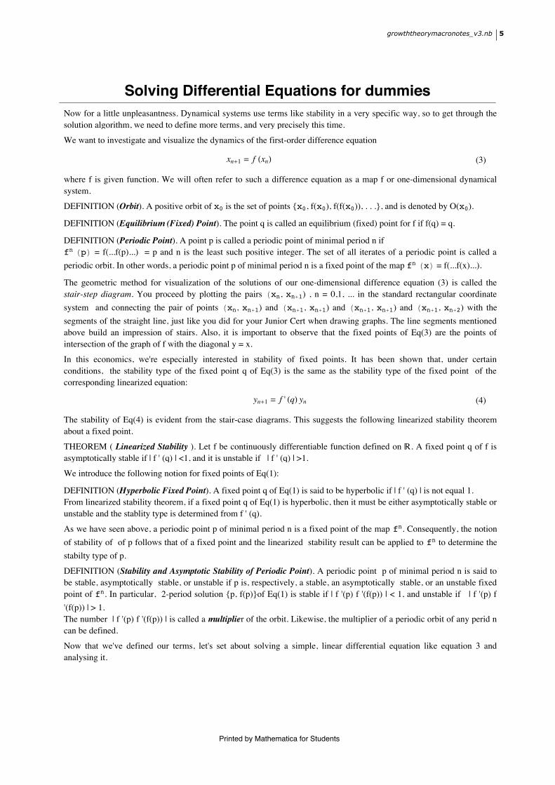
points H-1, 0, 0L, H1, 0, 0L, and H0, 1, 0L. Let's generate some graphs to see what this means in terms of level surfaces. First, we need our contraint surface, which

is just a sphere of radius one centered at the origin.



constraint = ContourPlot3D@g@x, y, zD, 8x, -1, 1<, 8y, -1, 1<,8z, -1, 1<, Contours Ø 81<,Axes Ø True, Lighting Ø Automatic, ContourStyle Ø 8RGBColor@0, 1, 0D<D

Now, we need the level surfaces of the function. First, let's generate the level surface for the maximum, which occurs

when f Hx, y, zL = +1.



levelsurfacemax = ContourPlot3D@f@x, y, zD, 8x, -2, 2<, 8y, -2, 2<,8z, -2, 2<, Contours Ø 81<, Axes Ø True, Lighting Ø Automatic,

ContourStyle Ø 8RGBColor@0, 0, 1D<D

Show@levelsurfacemax, constraint, ViewPoint Ø 85, -5, 2<,AxesLabel Ø 8x, y, z<D

We know that graphically , what must be happening is the tangent plane to the constraint surface must be the same as

the tangent plane to the level surface of the function at the points where they touch. From the above diagram, we can

see that this occurs for the points H-1, 0, 0L, H1, 0, 0L, and H0, 1, 0L, as expected. What would happen if we decreased the

level surface of the function slightly? We would expect the constraint surface to "poke through", and they would not

have the same tangent planes where they touched. Let's try it.



We know that graphically , what must be happening is the tangent plane to the constraint surface must be the same as

the tangent plane to the level surface of the function at the points where they touch. From the above diagram, we can

see that this occurs for the points H-1, 0, 0L, H1, 0, 0L, and H0, 1, 0L, as expected. What would happen if we decreased the

level surface of the function slightly? We would expect the constraint surface to "poke through", and they would not

have the same tangent planes where they touched. Let's try it.

levelsurface1 = ContourPlot3D@f@x, y, zD, 8x, -2, 2<, 8y, -2, 2<,8z, -2, 2<, Contours Ø 80.8`<, Axes Ø True, Lighting Ø Automatic,

ContourStyle Ø 8RGBColor@1, 0, 0D<DShow@levelsurface1, constraint, ViewPoint Ø 85, -5, 2<,AxesLabel Ø 8x, y, z<D;

True

True

The constraint curve is poking through the side. Although we can't see it, we know that it is also poking through in the

back and on the other side as well. Now at any point of contact between the two surfaces the tangent planes are not the

same. If we had increased the level surface of the function to f Hx, y, zL = k, k > 1, then the surfaces would not touch.

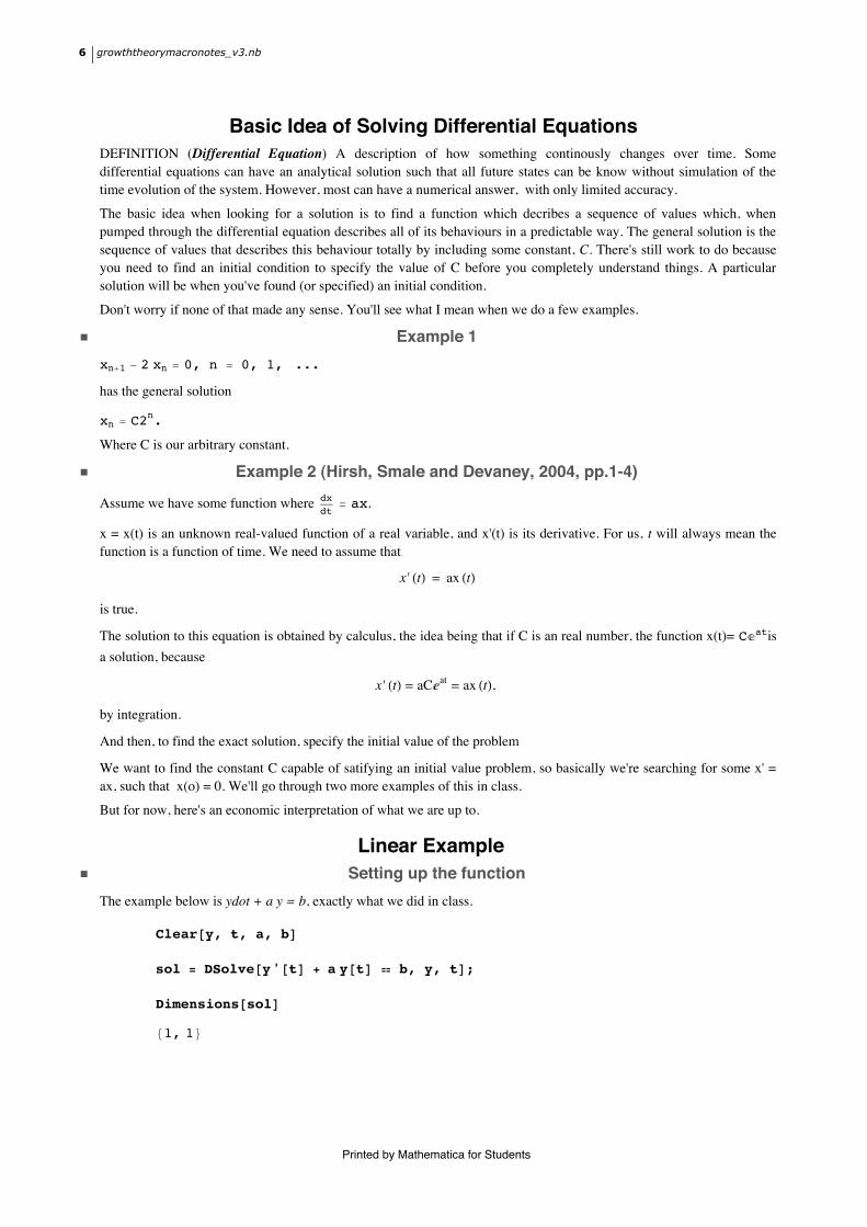
Let's look at the minimum level surface now, where f Hx, y, zL = -1.



levelsurfacemin = ContourPlot3D@f@x, y, zD, 8x, -5, 5<, 8y, -5, 5<,8z, -5, 5<, Contours Ø 8-1<, Axes Ø True, Lighting Ø Automatic,




Show@levelsurfacemin, constraint, ViewPoint Ø 85, 0, 1<D

Here the level surface of the function is encompasing the surface fo the constraint. We can see that the two surfaces

touch at the points H0, 0, -1L, H0, 0, 1L, and H0, -1, 0L, and also have the same tangent plane at those points. If we

increased the level surface of the function, we would again find that the constraint surface would poke through the

surface. If we decreased the level curve, then the two srufaces would not touch.

As for the extraneous values, let's generate a plot of the level curve for one of them. The 0.851 is really 23/27, so we

need a level surface for the function at this value.



levelsurface2 = ContourPlot3DBf@x, y, zD, 8x, -2, 2<, 8y, -2, 2<,

8z, -2, 2<, Contours Ø :2327

>, Axes Ø True, Lighting Ø Automatic,

ContourStyle Ø 8RGBColor@1, 0, 0D<FShow@levelsurface2, constraint, ViewPoint Ø 85, 5, 2<D

We see that the constraint surface and the level surface do indeed meet at a point that has a common tangent plane--

however, the constraint surface is poking through elsewhere. This tells us that althought the conditions of the Lagrange

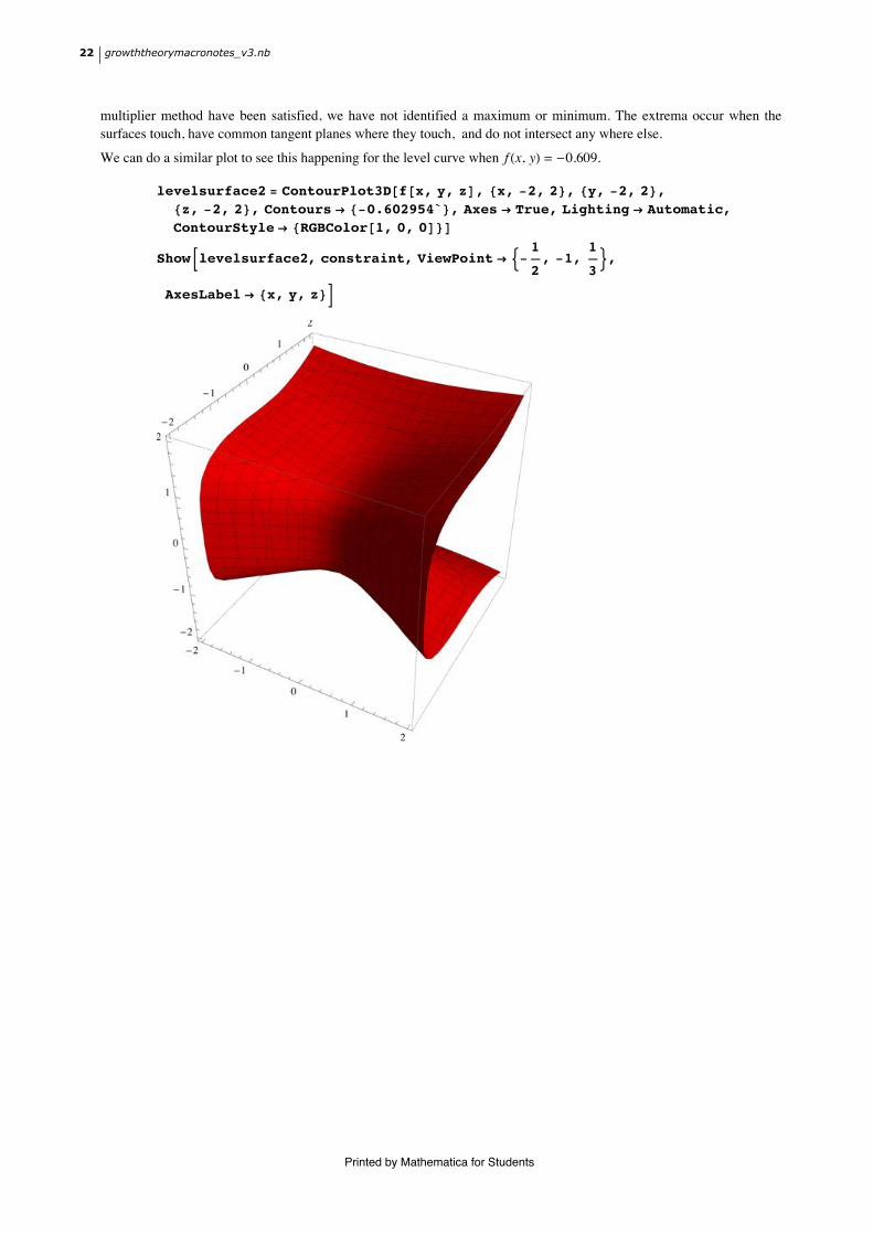
multiplier method have been satisfied, we have not identified a maximum or minimum. The extrema occur when the

surfaces touch, have common tangent planes where they touch, and do not intersect any where else.



We see that the constraint surface and the level surface do indeed meet at a point that has a common tangent plane--

however, the constraint surface is poking through elsewhere. This tells us that althought the conditions of the Lagrange

multiplier method have been satisfied, we have not identified a maximum or minimum. The extrema occur when the

surfaces touch, have common tangent planes where they touch, and do not intersect any where else.

We can do a similar plot to see this happening for the level curve when f Hx, yL = -0.609.

levelsurface2 = ContourPlot3D@f@x, y, zD, 8x, -2, 2<, 8y, -2, 2<,8z, -2, 2<, Contours Ø 8-0.602954`<, Axes Ø True, Lighting Ø Automatic,


ShowBlevelsurface2, constraint, ViewPoint Ø :-1

2, -1,

1

3>,

AxesLabel Ø 8x, y, z<F



Just because I'm a geek, let's get the cool rotational version of this last sketch. Richt click and drag the image to rotate it.



levelsurface2 = ContourPlot3D@f@x, y, zD, 8x, -2, 2<, 8y, -2, 2<,8z, -2, 2<, Contours Ø 8-0.602954`<D

Show@levelsurface2, constraintD

Dynamic Programming



Dynamic ProgrammingIt also seems reasonable to postulate an interdependence be-tween the variables entering an economic system in the case con-cerning the determination of the conditions for correctly anticipated processes. These conditions are that the individuals have such expectations of the future that they act in ways which are necessary for their expectations to be fulfilled.It follows that the interdependence between present and future magnitudes is conditioned in this case by the fact that the latter,via correct anticipations, influence the former.If we also choose to describe such developments as equilibrium processes, this implies that we widen the concept of equilibrium to include also economic systems describing changes over time where the changes that take place from period to period do not cause any interruption in, but, the contrary, are an expression of the continual adjust-ment of the variables to each other.

Lindahl (1954), p.27.

The above quote is the best example I can find of an intuitive explanation forwhydynamic programming is needed in

neoclassical economics.We can define dynamic programming as "a method of solving multi-stage problems in which

the decisions at one stage become the conditions governing the succeeding stages"

(www.indiainfoline.com/bisc/jama/jmmd.html ), but what we need to see is the economic rationale for the technique.We

use dynamic programming because the economic problem is to maximise the value of the processes run in the economy

through time. So,we need a method that performs the Lagrangian analysis I've just shown you at various intervals

throughout time.The solution should be expressed as a function of time.

The economic problem faced by neoclassical economists is: what processes should be run now and later in order to

maxmise the value of resources used throughout the lifetime of the economy. The way to do this is to produce a

functional that can iterate each shadow price over time to get the optimal solution. The planner interested in optimal

growth must thus form the Hamiltonian.

The Hamiltonian technique performs exactly the same role of converting constrained extrema problems to unconstrained

extrema ones as the Lagrange multiplier shown above, but it does it dynamically, in the sense that it captures

interactions of past values of the constraint (now called the control) variable(s) with the present and future values of the

objective (now called state) variable(s) via the use of an operator, exactly like the familiar l, but here called the costate

variable(s). The Lagrangian l finds the maximum value of the objective function which satisfies the constraint in each

single period, while the costate variable attaches a value to the next period's production/consumption/investment, which

must be zero at the end of time. To set up a Hamiltonian problem, therefore, we require a description of the state of the

system at some initial point, called the initial condition, and a description of the end of the system, called the

transversality or boundary condition, which I will say more about in the lecture. Then, we need a function which

assigns values to the state variable at each moment, given the value of the control. So, for the (Ramsey-esque) case of

maximizing utility subject to a consumption and labour force constraint, the set up of the problem will go something like

this.

Hamiltonians, a Step by Step Guide

ü Step One. Form the Hamiltonian

(9)H = Max ‡0

¶

‰-rt LHtL. u@CHtLDnHtL „ t,

With L(t) being the labour force, C(t) its consumption, n(t) the growth rate of the population, and r a measure of the

discount rate. What this does is to set the pure discount rate, e, proportional to an increasing weight of the level of a

future population.

Intuitively, what this means is that when the population is bigger, utility will increase by the number of people existing

in that later period. This is quite a Benthamite argument, in my view. Let's allow our initial labour force to be one, and

cap population growth at n(t) = n. Things aren't that rosy, though, as we have to consider the level of (per capita) capital

accumulation at any time, which is given by

(10)H = ‡0

¶

‰-Hr-nL t nHtL „ t,

s.t. k°

< f Hk HtLL - C HtL - nkHtL .

(Think of this as a budget constraint for the State variable )



We have our initial (or boundary) condition,

k H0L = k0,

And our transversality condition,

m HtL = 0

What does the transversality condition mean? Imagine you wish to optimally save over some finite horizon, say the time

of your life. Will you save in the last period? Most likely not. The transversality condition supplies another boundary,

where the costate variable returns a value to the previous period of zero. The rocket, if the control variable is fuel

fuelling a rocket, and the state variable is the velocity and position of the rocket should run out of fuel just as it hits its

target and goes boom.

ü Step Two

We partially differentiate H(‰) with respect to the costate and state variables. The punchline before the joke is told is: in

order to get the integrand to converge at all, the profit rate must be greater than the level of population growth. This has

enormous implications. This analysis uses Pontryagin's maximum and minimum principles, which ensure convergence

when h = e - n, h > 0. Forming the Hamiltonian in the same way as the Lagrangian, we get

H = ‰-ht uHCL + mH f HkHtL - CHtL - nkHtLL.ü Step Three

Take the partial derivatives of this equation to find that

! H

!C= 0 fl u' - ‰ht m,

u°

= ! H

!k= - uI f ' - nM

We get a differential equation for the costate variable m, which is paired with

k°

= H f HkHtLL - CHtL - nkHtL.These are Euler (pronounced 'Oy-Ler') equations which give us a 2*2 system of differential equations, solvable in the

usual way. We'll look at the 'usual way' in the next section.

Points to note are:

1. equation (6) is running backward in time, because of the minus sign.

2. equation (7) is running forward in time.

So, Hamilton has given us a system running both backwards and forwards in time, a 2-point boundary value problem,

expressed in (usually finite) time. The m values are transmitting information backward in time about what the resource

situation is there. It turns out that the system is most efficient computationally when both are allowed to move forward

and backward in time.

ü Steps Four and Five

To 'close' the model, all we need to do is specify the shape of the utility function (usually Constant Elasticity of

Substitution, CES) as we do below in several examples, and step five, we assess the stability of the model, meaning we

try to determine in what range and over what domain the function varies, how it varies, and what we might expect it to

do given some arbitrary input of values||converge to a point, cycle endlessly, or explode, or a combination of these.

Setting the value of our utility function to equal something like

u HC HtLL = :C1-r

1-r, r " 1

Log@CD, r = 1,

Then if Log[C] pertains, we have a Bernoulli utility function, where 1/r is the elasticity of substitution between two

points in time. Intuitively, if r >0, then we don't care about the present (we are immortal, anyway). You can also show

that



Then if Log[C] pertains, we have a Bernoulli utility function, where 1/r is the elasticity of substitution between two

points in time. Intuitively, if r >0, then we don't care about the present (we are immortal, anyway). You can also show

that

e + r.C`

= f ',

which says (dropping the t-subscript for clarity) that the pure discount rate and the growth rate of consumption per head

C`, all weighted by r is equal to f ', the marginal product of capital. This is the Keynes- Ramsey rule, which means that

the economy can account for and solve the problem of different wants and provisions, as Bohm-Bawerk put it, by seeing

how fast utility per person is changing over time, and adjusting the speed of production to accommodate this. The

importance of such a finding does not need much comment, as it should be obvious.

There are problems, however. Under realistic descriptions of utility and uncertainty~stochastic income and habit formation~

these intertemporal problems are very difficult to solve. As Velupillai (2000, cht 8) shows, these techniques are based upon

mathematical machinery called Pontryagin Maxima, which have serious flaws in their constructive interpretations. All of this is a

long winded way of saying these models are hard to compute except under very restrictive assumptions.

Optimizing agents must build up precautionary savings to buffer bad income realizations, and must anticipate the negative

“internality” of current consumption on future utility, through habits. Here we will look at an unrealistic, 1960's version of the

system of optimal growth studied by Cass and Koopmans, the exposition of which is in Barro & Sala-i-Martin, 2004, chapter 2, as

well as Romer, 2004, chapter 2.

It is historically significant that the first model of this type was studied by the Cambridge philosopher F.P. Ramsey (1929),

using a technique called the calculus of variations. Ramsey's idea was that as societies advanced through technological progress,

there would be such a build up of the capital stock, causing a falling rate of profit, that capital accumulation as an activity would

just go away as the profit motive could not be satisfied at such low rates of profit growth for such high levels of capital input.

Ramsey's steady state is thus not a steady state as we understand it today, but rather a 'state of bliss', wherein the cultural context for

capital accumulation is destroyed by the existence of overweening wealth. We would say these lucky souls have their utility

functions saturated, thus consumption growth flatlines. This idea is formally equivalent with Keynes' 'Euthanasia of the Rentiers'

notion, discussed in his general theory.

"you can't just draw a demand and supply curve for capital and apply the usual apparatus of saver's rent etc.; e.g. the treatment of saving as a use of income with its own elasticity of demand (as in Pigou Public Finance p. 138) is not really right. I did a very elabourate treatment of taxation and savings which was cut out by Maynard; rightly as it was too involved in comparison with the conclusions which were feeble. ...I first started thinking about saving through being dissatisfied with Pigou's treating it in this way; but now I think what he says is good enough perhaps, as anything better would be so complicated and fruitless." |||Letter from Frank Ramsey to Roy Harrod, (1929)

Below, in the optimal Cass-Koopmans growth model we will study, the utility does not saturate at all, but rather

increases without bound. As we shall see, another element 'closes' the system for the lucky Neoclassical modeler,

willfully (or blissfully: it depends) ignorant of computability considerations.

ü Exercise 5

There is a very large number of households with perfect foresight, ordered on the [0,1] interval. A given household, of

size L, will grow at a rate n. Each person is endowed with one unit of labour per period of time, and the household

income of the model is made up of labour income (obviously dependent on the wage rate, w) plus the net real rate of

return (r - d) on the capital they employ per period, K. Each household wants to maximise the value of an infinite utility

stream, Ÿ0

¶u HcL, with each generation taking into account the welfare of its descendants (via the transversality

conditions we derived in class. Form the Maximisation problem.

Examples of Dynamic Programming: the Ramsey-Cass Koopmans Model

Assume a representative agent household. A representative agent is one whose preferences are copied throughout the

economy, thus we need only look at one household in the aggregate. Our 'macro economy' thus consists of a simple

addition of the outputs of a continuum of identical households of size L, which we will allow grow at a rate n. Each

person is endowed with one unit of labour per period of time, and the household income of the model is made up of

labour income (obviously dependent on the wage rate, w) plus the net real rate of return (r - d) on the capital they

employ per period, K. Each household wants to maximise the value of an infinite utility stream, with each generation

taking into account the welfare of its descendents via transversality conditions in exactly the way Ramsey (1929)

described to Harrod as being incorrect (see quote above). We can express this intertemporal maximisation as:



Max8c<

U0 = ‡0

¶

uHcL ‰-rt „ t

s.t. K°

= Hr - dL K + wL - cL

KH0L = K0

0 b cL b Hr - dL K + wL.

The utility function being maximised is usually of the Constant Elasticity of Substitution (CES) form, modified with

intertemporal assumptions (which is the cause for Ramsey's misgivings), so it looks like:

u HcL =c1-s - 1

1 - s, with c, s > 0

Table of Variables and their meanings

Variable Meaning

U Total Utility of household

c level of consumption

K capital stock per period

r return on capital Hrental priceLd capital depreciation

r elasticity of demand wrt consumption

-s elasticity of utility wrt consumption

What does this look like? Here I plot three utility functions with different values of s for comparison.

s1 = 0; s2 = 1.1`; s3 = 3;

PlotB:c1-s1 - 1

1 - s1,c1-s2 - 1

1 - s2,c1-s3 - 1

1 - s3>, 8c, 0, 5<,

PlotStyle Ø [email protected]`D, RGBColor@1, 0, 0D<,[email protected]`D, RGBColor@0, 0, 1D<, [email protected]`D,RGBColor@1, 0, 0D<, PlotRange Ø 8-2, 2<, AxesLabel Ø 8"c", "uHcL"<F

1 2 3 4 5c

-2

-1

1

2

uHcL

The marginal utility of consumption is u'(c) = c-s . The elasticity of the marginal utility relative the amount consumed is

-s. To get our maximisation on, though, we need to set up a current value Hamiltonian (Here we are doing this

according to Shell's article on Hamiltonians in the New Palgrave, referenced below):

(11)H Hc, K, lL =c1-s - 1

1 - s+ l@ Hr - dL K + wL - cL D

Derive the first order conditions of the system in the usual way to obtain:

(12)Hc = c-s - lL = 0 ó C-s

= lL1-s



l°

= -HK + rl = -lHr - dL + rl ól°

l= r - r + d

K°

= Hl = Hr - dL K + wL - C

Limtö¶

‰-rt l HtL K HtL = 0ó - r + Limtö¶

l°

+ Limtö¶

K°

< 0

Now just differentiate C-s

= lL1-s

(called the necessary condition) with respect to time and sub in the fact that

l°

l= r - r + d, (called the costate equation) and we have the Ramsey-Cass-Koopmans rule of optimal consumption:

(13)C°

=C

s@r - d - r - H1 - sL nD

So What?

So what? Who cares about this measure? What does it mean? Firstly, is says that the household's borrowing solution is

simple: just borrow up until u'(c) = 0, which is a restatement of the Keynes-Ramsey Rule derived and described above.

Second, When one uses the Hamiltonian method to consider optimal production as well, there is a significant policy

proposition: the Hamiltonian method implies that policy over the (infinitely) long run is inefficient, because it would

take away resources that might have been used to jump the economy onto its balanced growth path.

The stationary solution of the system is defined by C°= K

°= 0. This stationary solution gives the level of the maximal

balanced level of utility over time, constrained by w, L and r.

variables = 8C, K<;equations = :Hr - dL*K + w *L - C ã 0,

C

s*Hr - d - r - H1 - sL*nL ã 0>;

sol = Solve@equations, 8C, K<D êê FullSimplify;

sol1 = sol@@1DD;

statpoint = 8csol, ksol< = variables ê. sol1

:0, L w

-r + d>

Stability Analysis of the Pure Ramsey Model

As you can see from reading Romer (2006), the Ramsey model of economic growth is a workhorse of

contemporary macro-economics. It is the starting point not only for growth theory but also for real business cycle

theory. Ask an economist how the economy will react to an increase in government purchases or to a change in the tax

rate on capital and the first model he or she will reach for in a search for answers is the Ramsey model.

The model requires that we solve two paired differential equations with a boundary condition. The solution

methods used, the shooting and time elimination method, are of wide applicability and may be of interest to researchers

in fields other than economics.

Since the Ramsey model is well known I will focus on how Mathematica can be used to solve the model.

Introductions to the Ramsey model can be found in the texts of Romer (1996), Barro and Sala-i-Martin (1995), and

Blanchard and Fischer (1989) and of course the original articles by Ramsey (1928), Cass (1965), and Koopmans (1965).

My notation again follows Romer's.

Assume a large number of identical firms. Each firm uses capital, K, and labour, L to produce output Y,

according to the production function Y = F@K, A µ LD. The parameter A measures the state of "technology."

Technology allows L workers to produce as if there were actually A µ L workers. We will assume that A grows

exogenously at the rate g, and simply designate the parametrized labour variable by AL.

Profit-maximizing firms hire capital and labour in competitive markets which they use to produce output. The

price of output is normalized to 1 which implies that a firm's profit function can be written as below where w is the

wage rate of effective labour, r is the interest rate and d the depreciation rate on capital. To be competitive with other

assets capital must pay its owners a return of r + d which is therefore the rental rate or interest rate on capital.



Assume a large number of identical firms. Each firm uses capital, K, and labour, L to produce output Y,

according to the production function Y = F@K, A µ LD. The parameter A measures the state of "technology."

Technology allows L workers to produce as if there were actually A µ L workers. We will assume that A grows

exogenously at the rate g, and simply designate the parametrized labour variable by AL.

Profit-maximizing firms hire capital and labour in competitive markets which they use to produce output. The

price of output is normalized to 1 which implies that a firm's profit function can be written as below where w is the

wage rate of effective labour, r is the interest rate and d the depreciation rate on capital. To be competitive with other

assets capital must pay its owners a return of r + d which is therefore the rental rate or interest rate on capital.

profit = F@K, ALD - w AL - Hr + dL K;To maximize profit the firm hires capital and labour until the first derivatives of the profit function with respect

to capital and labour respectively are zero.

D@profit, KD == 0

-r - d + FH1,0L@K, ALD ã 0

D@profit, ALD == 0

-w + FH0,1L@K, ALD ã 0

We will also assume that the production function F is linearly homogeneous or in economic terms that it

exhibits constant returns to scale (CRS). The CRS assumption means that if inputs increase by a factor of c, output will

also increase by a factor of c, F@cK, cALD = cF@K, ALD. Euler's theorem says that if F@K, ALD is linearly

homogeneous, then Y = FK K + FAL AL. Using the above first-order conditions, Euler's theorem implies that factor

payments exhaust the product, Y = Hr + d L K + w AL. Setting c = 1 êAL allows us to write the production function in

terms of one variable, capital per unit of effective labour k = K êAL. Thus, output per unit of effective labour can be

written Y êAL = y = f @kD. Rewriting the first-order condition for capital we have, as before

r + d = f '@kDand using (1) and Euler's theorem

w = f @kD - kf '@kD.Household behavior is more complicated. There are a large number, H, of identical households. Each member

of the household supplies 1 unit of labour at every point in time. Households own the capital stock, which they rent to

firms. Each household begins with capital holdings of K[0]/H where K[t] is the amount of capital at time t. At each

moment in time the household chooses how to divide its income - from wages and the renting of capital - between

consumption and savings in order to maximize lifetime utility. The household's lifetime utility is written;

U = ‡0

¶

e-rt uHC@tDL L@tD êH dt

where C@tD is the consumption of each household member at time t. u@C@tDD is the instantaneous utility created by the

consumption of C@tD at time t. L[t] is the total population of the economy and L[t]/H the number of members of the

household at time t. r > 0 is the household's discount rate (assumed the same for all households). The higher is r the

more the household discounts future consumption relative to current consumption. It is common to assume that

instantaneous utility is of the form uHC@tDL =C@tD1-q

1-q, with q > 0 and r - n - H1 - qL g > 0. q governs how willing

individuals are to substitute consumption from one time period into another. A lower q implies a greater willingness to

substitute consumption tomorrow for consumption today. The condition r - n - H1 - qL g > 0 is a technical condition

needed to ensure that utility is bounded below infinity. It's convenient to write the budget constraint in terms of

consumption per unit of effective labour. After some algebraic manipulations and taking into account the fact that L and

A are growing we have (see Romer (1996) for the derivation).

U = B ‡0

¶

e- bt c@tD1-q

1 - qdt



where B = A@0D1-q L@0D êH and

b = r - n - H1 - qL g.

.

B is an unimportant constant and will be normalized to 1 in what follows.

The household faces two constraints when maximizing utility.

k '@tD = r@tD k@tD + eHn+gL tHw@tD - c@tDL

Limtö¶

e-R@tD eHn+gL t k@tD ¥ 0,

where R@tD = ‡0

t

r@tD dt.

The first constraint is closer to an accounting identity than a constraint it that it says that the growth in the

household's capital stock (per unit of effective labour) is equal to the interest earnings on the current capital stock plus

the difference between the household's wages in period t and its consumption in period t (the exponential term adjusts

for growth in effective labour). Notice that 1) does not forbid the household from consuming more than its wages by

borrowing (creating a negative capital stock). It follows that the optimal solution to the household's problem is to

borrow an infinite amount and live it up! Since the latter strategy is unrealistic, we need constraint 2, which says that

the household's capital stock (adjusted per unit of effective labour) cannot be negative in the limit. In other words, the

household must live within its means, if not on any given day then in the limit.

The household's problem has been set up as a standard problem in optimal control theory that can be solved

using the method of Hamiltonians (see the references section or Kamien and Schwartz, (1981) for an introduction to

optimal control theory). Write the Hamiltonian as:

H = E-b t c@tD1-q

1 - q+ l@tD Ir@tD k@tD + EHn+gL t Hw@tD - c@tDLM

‰-t b c@tD1-q

1 - q+ Ik@tD r@tD + ‰Hg+nL t H-c@tD + w@tDLM l@tD

Optimal control theory tells us that the solution to our maximization problem must satisfy Hc = 0, Hk = -!lHtL!t

and the transversality condition LimtØ¶l(t)k(t)Ø0. (It can be shown that the transversality condition implies that the no

infinite debt constraint of the household's problem will be satisfied in equilibrium, see Barro and Salai-i-Martin, 1995).

Hc = D@H, c@tDD == 0

‰-t b c@tD-q - ‰Hg+nL t l@tD ã 0

Hk = D@H, k@tDD == -D@l@tD, tDr@tD l@tD ã -l£@tD

We now rearrange the first-order conditions to find a particularly convenient representation. First solve Hc for

l(t) then differentiate with respect to t.

sol1 = Solve@Hc, l@tDD êê Simplify

99l@tD Ø ‰-t Hg+n+bL c@tD-q==

sol2 = D@sol1, tD

99l£@tD Ø ‰-t Hg+n+bL H-g - n - bL c@tD-q - ‰-t Hg+n+bL q c@tD-1-q c£@tD==

Now divide sol2 by sol1 and simplify.



Now divide sol2 by sol1 and simplify.

tmp = sol2@@1, 1, 1DDêsol1@@1, 1, 1DD == sol2@@1, 1, 2DDêsol1@@1, 1, 2DD êêSimplify

g + n + b +q c£@tDc@tD +

l£@tDl@tD ã 0

From the first-order condition for Hk we can make the substitution l£HtL

lHtL-> -r@tDand from the definition of b

we can make the substitution b->r-n-(1-q)g.

tmp = tmp ê. l£HtLlHtL

-> -r@tD

g + n + b - r@tD +q c£@tDc@tD ã 0

Solve@tmp, c'@tDD

::c£@tD Ø -c@tD Hg + n + b - r@tDL

q>>

% ê. 8b -> r - n - H1 - qL g< êê Simplify

::c£@tD Ø -c@tD Hg q + r - r@tDL

q>>

Rearranging we have:

tmp = c'@tDêc@tD ==H rHtL - r - g qL

q

c£@tDc@tD ã

-g q - r + r@tDq

Using the fact that in equilibrium, r[t]==f'[k[t]]-d we have:

tmp = tmp ê. r@tD -> f'@k@tDD - d

c£@tDc@tD ã

-d - g q - r + f£@k@tDDq

The dynamics of k are determined from the accounting identity that changes in the capital stock equal

production minus consumption minus depreciation (with suitable adjustments for changes in the stock of effective

labour).

k'@tD == f@k@tDD - c@tD - Hn + g + dL k@tDk£@tD ã -c@tD + f@k@tDD - Hg + n + dL k@tD

The two key equations of the Ramsey model are thus :

1. c£HtL = cHtL f £HkHtLL - d - r - g f

fand

2. k£HtL == f HkHtLL - cHtL - Hg + n + dL kHtL

Numerically Solving the Model



Numerically Solving the Model

We now turn to numerically solving the model for steady states and transition paths. To do so we specify that

the production function is of the Cobb|Douglas form, f HkHtLL = kHtLa. Now define CPrime and KPrime as follows:

In[20]:= Clear@a , d , g , r , q, x, y, a, b, k, tD

In[21]:= CPrime@a_, d_, g_, r_, q_D := c@tD Ha k@tD^Ha - 1L - d - r - g qLêq

In[22]:= KPrime@a_, d_, g_, n_D := k@tD^a - c@tD - Hg + n + dL k@tDWe initially set a=1/3, d=.05, g=.02, n=0.01, r=.02, and q=1.75. We now solve for the

steady state, the levels of c and k such that c'[t]=k'[t]=0.

In[23]:= kbar1 =

k@tD ê. Flatten ü Solve@CPrime@1ê3, 0.05, 0.02, 0.02, 1.75D == 0.0, k@tDDOut[23]= 5.65632

In[24]:= cfunct = c@tD ê. Flatten ü Solve@KPrime@1ê3, 0.05, 0.02, 0.01D == 0.0, c@tDD

Out[24]= -1. I0. - 1. k@tD1ê3 + 0.08 k@tDM

In[25]:= cbar1 = cfunct ê. k@tD -> kbar1

General::spell1 :

New symbol name "cbar1" is similar to existing symbol "kbar1" and may be misspelled. à

Out[25]= 1.32924

In[26]:= p1 = Plot@cfunct ê. k@tD -> k, 8k, 0.01, 10<, DisplayFunction -> IdentityD;The next figure shows the steady state levels of capital and consumption.

In[27]:= SS = Show@p1, Graphics@8Line@88kbar1, 0<, 8kbar1, 1.7`<<D<D,AxesLabel Ø 8"K Stock", "Consumption"<,DisplayFunctionØ $DisplayFunctionD

Out[27]=

2 4 6 8 10K Stock

0.8

0.9

1.0

1.1

1.2

1.3

Consumption

Transition Dynamics

Suppose that we start off with a capital stock less than the steady state capital stock. How does the economy

evolve through time? A Phase Plot gives us the answer.

The "fish field" tells us both the direction and strength of the flow. Notice that the flow is stronger the farther

the system is from the k'[t]=0 or c'[t]=0 lines and in particular that the flow is slowest nearest the equilibrium point. The

field also tells us something interesting about the solution to the consumer's maximization problem. Suppose that the

capital stock starts at 1. If consumption is too low then according to the dynamics, households begin to add to their

capital stock. They keep adding to the capital stock even as consumption begins to fall. Eventually consumption

approaches zero and the capital stock approaches a large constant (the k where k'[t]=0 intersects the x axis). Intuitively,

this path cannot be optimal. Households could attain higher utility by consuming some of their capital horde! (More

technically, it can be shown that capital hoarding violates the transversality condition). If consumption starts too high,

however, the dynamics indicate increasing consumption financed with a falling capital stock. Eventually the capital

stock is fully consumed and consumption crashes to zero. But this too cannot be optimal. Even if it were optimal for

the households to consume all of their capital stock they would never do it in a way which requires a consumption

crash~they would seek to smooth consumption instead. We can rule out any solution, therefore, that does not converge

to the steady state. To understand what happens when the capital stock starts away from the steady state we must solve

for a level of consumption such that the dynamics of the model lead exactly to the steady state. We demonstrate two

methods for solving this problem. First, the trial and error or shooting method and then the more elegant time

elimination method due to Mulligan and Salai-i-Martin (1991).



The "fish field" tells us both the direction and strength of the flow. Notice that the flow is stronger the farther

the system is from the k'[t]=0 or c'[t]=0 lines and in particular that the flow is slowest nearest the equilibrium point. The

field also tells us something interesting about the solution to the consumer's maximization problem. Suppose that the

capital stock starts at 1. If consumption is too low then according to the dynamics, households begin to add to their

capital stock. They keep adding to the capital stock even as consumption begins to fall. Eventually consumption

approaches zero and the capital stock approaches a large constant (the k where k'[t]=0 intersects the x axis). Intuitively,

this path cannot be optimal. Households could attain higher utility by consuming some of their capital horde! (More

technically, it can be shown that capital hoarding violates the transversality condition). If consumption starts too high,

however, the dynamics indicate increasing consumption financed with a falling capital stock. Eventually the capital

stock is fully consumed and consumption crashes to zero. But this too cannot be optimal. Even if it were optimal for

the households to consume all of their capital stock they would never do it in a way which requires a consumption

crash~they would seek to smooth consumption instead. We can rule out any solution, therefore, that does not converge

to the steady state. To understand what happens when the capital stock starts away from the steady state we must solve

for a level of consumption such that the dynamics of the model lead exactly to the steady state. We demonstrate two

methods for solving this problem. First, the trial and error or shooting method and then the more elegant time

elimination method due to Mulligan and Salai-i-Martin (1991).

Suppose k[0]=1, the shooting method picks an arbitrary initial consumption level, c[0]=a and asks whether given

k[0]=1 and c[0]=a the solution path converges to the steady state. Below we solve the model given two possible initial

levels of consumption c[0]=0.6 and c[0]=0.7.

In[44]:= sol1 = NDSolve@8c'@tD == CPrime@1ê3, 0.05, 0.02, 0.02, 1.75D,k'@tD == KPrime@1ê3, 0.05, 0.02, 0.01D, c@0D == 0.55, k@0D == 1<,

8c@tD, k@tD<, 8t, 0, 150<D;

In[45]:= sol2 = NDSolve@8c'@tD == CPrime@1ê3, 0.05, .02, .02, 1.75D,k'@tD == KPrime@1ê3, .05, .02, .01D, c@0D == 0.65, k@0D == 1<,

8c@tD, k@tD<, 8t, 0, 150<D;NDSolve::ndsz :

At t == 13.017352193778757 ,̀ step size is effectively zero; singularity or stiff system suspected. à

In[46]:= p1 = ParametricPlot@Evaluate@8k@tD, c@tD< ê. sol1D, 8t, 0, 25<,DisplayFunction -> IdentityD;

In[47]:= p2 = ParametricPlot@Evaluate@8k@tD, c@tD< ê. sol2D, 8t, 0, 7.8<,DisplayFunction -> IdentityD;

In[48]:= Show@SS, p1, p2D

Out[48]=

2 4 6 8 10K Stock

0.8

0.9

1.0

1.1

1.2

1.3

Consumption

Neither candidate solution converges to the steady state. The first implies capital hoarding and eventually zero

consumption. The second implies that the capital stock goes to zero and that consumption crashes. From the phase plot,

however, it appears that a solution exists somewhere in between c[0]=0.55 and c[0]=0.65 which will converge exactly

(or arbitrarily closely) to the steady state. The following code uses FindRoot to arrive at an approximate solution.

In[49]:= system@a_D :=

NDSolve@8c'@tD == CPrime@1ê3, 0.05, 0.02, 0.02, 1.75D,k'@tD == KPrime@1ê3, 0.05, 0.02, 0.01D, c@0D == a, k@0D == 1<,

8c, k<, 8t, 0, 100<D ;



In[50]:= gun := c@system@Ò1D@@1, 1, 2, 1, 1, 2DDD ê. system@Ò1D@@1, 1DD &

In[51]:= init = a ê. FindRoot@gun@aD == cbar1, 8a, 0.55, 0.65<, AccuracyGoal -> 4,

MaxIterations -> 35D;NDSolve::ndinnt : Initial condition a is not a number or a rectangular array of numbers. à

Part::partd : Part specification NDSolve@á1àDP1, 1, 2, 1, 1, 2T is longer than depth of object. à

NDSolve::ndinnt : Initial condition a is not a number or a rectangular array of numbers. à

ReplaceAll::reps :

:c£@tD ã 0.571429c@tD -0.105+1

3k@tD2ê3> is neither a list of replacement rules nor a valid

dispatch table, and so cannot be used for replacing. à

ReplaceAll::reps :

:c£@tD ã 0.571429c@tD -0.105+1



ReplaceAll::reps :

:c£@tD ã 0.571429c@tD -0.105+0.333333

k@tD2ê3> is neither a list of replacement rules nor a valid


General::stop : Further output of ReplaceAll::reps will be suppressed during this calculation. à

FindRoot::nlnum :

The function value 8-1.32924+ [email protected] ê. c£@tD ã 0.571429c@tD H-0.105+ 0.333333Power@á1àDLL<is not a list of numbers with dimensions 81< at 8a< = 80.55<.


General::stop : Further output of NDSolve::ndinnt will be suppressed during this calculation. à


FindRoot::nlnum :




In[52]:= p3 = ParametricPlot@Evaluate@8k@tD, c@tD< ê. system@initDD, 8t, 0, 50<,PlotStyle -> Hue@0D, DisplayFunction -> IdentityD;




ReplaceAll::reps :

:c£@tD ã 0.571429c@tD -0.105+1



ReplaceAll::reps :

:c£@tD ã 0.571429c@tD -0.105+1



ReplaceAll::reps :

:c£@tD ã 0.571429c@tD -0.105+0.333333

k@tD2ê3> is neither a list of replacement rules nor a valid



FindRoot::nlnum :



General::stop : Further output of NDSolve::ndinnt will be suppressed during this calculation. à


FindRoot::nlnum :



General::stop : Further output of Part::partd will be suppressed during this calculation. à

FindRoot::nlnum :


General::stop : Further output of FindRoot::nlnum will be suppressed during this calculation. à

NDSolve::dsvar : 0.0010204081632653062` cannot be used as a variable. à



General::stop : Further output of NDSolve::dsvar will be suppressed during this calculation. à



In[53]:= Show@SS, p1, p2, p3D

Out[53]=

2 4 6 8 10K Stock

0.8

0.9

1.0

1.1

1.2

1.3

Consumption

The Time Elimination Method

A more elegant way to solve these types of problems is the time elimination method (Mulligan and Sala-i-

Martin, 1991). With this method we solve for the c[k] function directly. Notice that !c

!të !k

!t=

!c

!k and recall that we

already know one point on the c[k] function, the steady state point, cê

= c@kD. With these two pieces of information we

can use NDSolve to find the entire c[k] function. First we define the derivative !c

!k.

In[93]:= deriv@k_D :=

CPrime@1ê3, 0.05, .02, .02, 1.75DêKPrime@1ê3, 0.05, .02, .01D ê.8c@tD -> c@kD, k@tD -> k<

At the steady state, the derivative is undefined, since by definition !c

!t=

!k

!t= 0. To get around this problem we

give NDSolve an initial condition which is just slightly different from the true steady state. [See Endnote 2.]

In[94]:= sol1 = NDSolve@8c'@kD == deriv@kD, c@kbar1D == cbar1 - .00001<, c,

8k, 0.01, kbar1<D;

In[95]:= PolicyF1 = c ê. sol1@@1DD;

In[96]:= p1 = Plot@PolicyF1@kD, 8k, 0.01, kbar1<, PlotStyle -> Hue@0D,DisplayFunction -> IdentityD;

In[97]:= Show@SS, p1D

Out[97]=

2 4 6 8 10K Stock

0.8

0.9

1.0

1.1

1.2

1.3

Consumption

If we are interested in the finding the function c[k] when k starts out above the initial state we solve:



In[98]:= sol2 = NDSolve@8c'@kD == deriv@kD, c@kbar1D == cbar1 + .001<, c,

8k, kbar1, 10<D;

In[99]:= PolicyF2 = c ê. sol2@@1DD;

In[100]:= p2 = Plot@PolicyF2@kD, 8k, kbar1, 10<, PlotStyle -> Hue@0D,DisplayFunction -> IdentityD;

In[101]:= Show@SS, p1, p2D

Out[101]=

2 4 6 8 10K Stock

0.8

0.9

1.0

1.1

1.2

1.3

Consumption

It will be convenient to collect both parts of c[k] into one function.

H*Clear@PolicyFunctionD*L

Time Paths

Often we are more interested in time paths than the "policy function" c[k]. We can solve for time paths using

the time elimination method as an intermediate step. Consider the function !k

!t= -cHtL - 0.08 kHtL + kHtL3

, although we

do not know the function c[t] we just solved for c[k[t]]. If we substitute c[k[t]] into !k

!t then with an arbitrary initial

condition c[x]==y we can numerically solve for the function k[t].

First define f=c[k[t]] using the solution found earlier.

In[102]:= f = c ê. sol1@@1DD

Out[102]= [email protected], 5.65632<<, <>D

Then in!k

! tsubstitute f@k@tDD for c@tD and solve using the initial condition k@0D = 1.

In[103]:= sol3 = NDSolve@8k'@tD == KPrime@1ê3, 0.05, .02, .01D ê. c@tD -> f@k@tDD,k@0D == 1<, k, 8t, 0, 65<D

Out[103]= 88k Ø InterpolatingFunction@880., 65.<<, <>D<<

In[104]:= KPath = k ê. sol3@@1DD

Out[104]= InterpolatingFunction@880., 65.<<, <>D

In[105]:= KPlot = Plot@KPath@tD, 8t, 0, 65<, DisplayFunction -> IdentityD;The figure below shows how the capital stock approaches its steady state value as a function of time.



In[106]:= Show@KPlot, Graphics@8Hue@0D, Line@880, kbar1<, 880, kbar1<<D<D,DisplayFunctionØ $DisplayFunctionD

Out[106]=

10 20 30 40 50 60

2

3

4

5

Suppose that a war cuts a nation's capital stock in half. Figures such as the previous one can be used to answer

questions like "How long will it take a nation to recover from the war" and "How fast will the economy grow along the

transition path?" (See for example King and Rebelo (1993).)

Since Y/L = Ay=Af[k] we can calculate the behavior of output per unit of effective labour along the transition

path.

In[107]:= yPath = KPath@tD^H1ê3L;

In[108]:= yPlot = Plot@yPath, 8t, 0, 65<, AxesLabel Ø 8"Time", "y"<D

Out[108]=

10 20 30 40 50 60Time

1.4

1.5

1.6

1.7

y

The economy's growth rate along the transition path is:

In[109]:= yGrowth = D@yPath, tDêyPath;

In[110]:= Plot@yGrowth, 8t, 0, 65<, AxesLabel Ø 8"Time", "y Growth Rate"<D

Out[110]=

10 20 30 40 50 60Time

0.005

0.010

0.015

0.020

0.025

0.030

0.035

y Growth Rate

Notice from above that the economy initially grows very quickly but then the growth rate slows as the economy

approaches the steady state. We can calculate half-life's and related data by using Mathematica's findroot function. (To

get the functions in appropriate form for FindRoot we define an intermediate function z).



Notice from above that the economy initially grows very quickly but then the growth rate slows as the economy

approaches the steady state. We can calculate half-life's and related data by using Mathematica's findroot function. (To

get the functions in appropriate form for FindRoot we define an intermediate function z).

In[116]:= z@x_D = yPath ê. 8t -> x<

Out[116]= InterpolatingFunction@880., 65.<<, <>D@xD1ê3

Taking z[65] as the steady state y and noting that y starts out at level 1 we find that it takes 6.1 years for output

to recover 1/2 of the war time loss.

In[117]:= FindRoot@z@tD == 1 + Hz@65D - 1Lê2, 8t, 2<D

Out[117]= 8t Ø 6.14073<

To solve for the time path of consumption, recall that !c

!t= 0.571429 cHtL J 1

3 kHtL2ê3- 0.105N. We can, therefore,

substitute k[t] using the function we have just found and then solve with an initial point. We choose the initial point for

consumption to be c[k[1]] so our consumption path will correspond to the capital path derived above.

In[118]:= sol4 = NDSolve@8c'@tD == CPrime@1ê3, 0.05, .02, .02, 1.75D ê. k@tD -> KPath@tD,c@0D == PolicyFunction@1D<, c, 8t, 0, 65<D

NDSolve::ndinnt :

Initial condition [email protected] is not a number or a rectangular array of numbers. à

Out[118]= NDSolveB:c£@tD ã

0.571429 c@tD -0.105 +1

3 InterpolatingFunction@880., 65.<<, <>D@tD2ê3,

c@0D ã PolicyFunction@1D>, c, 8t, 0, 65<F

In[91]:= CPath = c ê. sol4@@1DDReplaceAll::reps :

:c£@tD ã 0.571429c@tD -0.105+1

3á1à@tD2ê3, c@0D ã PolicyFunction@1D> is neither a list of

replacement rules nor a valid dispatch table, and so cannot be used for replacing. à

Out[91]= c ê. :c£@tD ã

0.571429 c@tD -0.105 +1


c@0D ã PolicyFunction@1D>



In[92]:= CPlot = Plot@CPath@tD, 8t, 0, 65<, AxesLabel Ø 8"Time", "Consumption"<DReplaceAll::reps :

8c£@0.00132786D ã [email protected], c@0D ã PolicyFunction@1D< is neither a list of replacementrules nor a valid dispatch table, and so cannot be used for replacing. à

ReplaceAll::reps :

8c£@0.00132786D ã [email protected], [email protected] ã [email protected]< is neither a list ofreplacement rules nor a valid dispatch table, and so cannot be used for replacing. à

ReplaceAll::reps :

8c£@1.32786D ã [email protected], c@0D ã PolicyFunction@1D< is neither a list of replacementrules nor a valid dispatch table, and so cannot be used for replacing. à


Out[92]=

10 20 30 40 50 60Time

-1.0

-0.5

0.5

1.0

Consumption

If we have proceeded correctly then in the steady state we should find that the difference between output and

consumption is just enough to keep the effective capital stock constant. Recall that to keep the effective capital stock

constant it must be increased by 8% every period. Using the values at t=65 as an approximation to the steady state we

can check this as follows:

In[114]:= HyPath ê. 8t -> 65<L - CPath@65DReplaceAll::reps :

:c£@tD ã 0.571429c@tD -0.105+1

3á1à@tD2ê3, c@0D ã PolicyFunction@1D> is neither a list of

replacement rules nor a valid dispatch table, and so cannot be used for replacing. à

Out[114]= 1.77952 - c ê. :c£@tD ã

0.571429 c@tD -0.105 +1


c@0D ã PolicyFunction@1D> @65D

In[115]:= KPath@65D*0.08

Out[115]= 0.450815

Thus we see that in the steady state savings are just equal to what is necessary to keep the effective capital stock

constant.



References (with hyperlinks)

Cormac O Gráda, A rocky road : the Irish economy since the 1920s, Manchester University

Press, 1997. Available here.

The Economy of Ireland : national and sectoral policy issues, 9th ed. edited by John O’Hagan

and Carol Newman, Dublin : Gill and Macmillan, 2005, available here.

Honohan, P. and Walsh, B Catching up with the Leaders: The Irish Hare, Brookings Papers on Economic Activity,

2002(1): 1-77. Working paper available at http://homepage.eircom.net/~phonohan/miracle.html.

Lindahl,Erik (1954), "On Keynes' Economic System", Economic Record, Vol.30, May, pp.19-32. Not available online.

In NUIG library, Economic Record back to 1964 (at the moment) is stored here.

K. V. Velupillai, (2000), Computable Economics, Oxford University Press, available here.

Jones, C. I. (1998) Introduction to Economic Growth, W.W. Norton & Co. Available here in 2nd Edition.

Alan Heston, Robert Summers and Bettina Aten, Penn World Table Version 6.2, Center for International Comparisons

of Production, Income and Prices at the University of Pennsylvania, September 2006., available here.

Barro, R. J. and X. Sala-i-Martin (1995). Economic Growth. New York: McGraw-Hill.

Blanchard, O. J., and S. Fischer. 1989. Lectures On Macroeconomics. Cambridge, Mass.: The MIT Press.

Cass, D. 1965. Optimum Growth in an Aggregative Model of Capital Accumulation. Review of Economic Studies

32:233-40.

Kamien, M. I., and N. L. Schwartz. 1991. Dynamic Optimization: The Calculus of Variations and Optimal Control in

Economics and Management. 2nd ed. Amsterdam: North-Holland.

King, R. G. and S.T. Rebelo. 1993. Transitional Dynamics and Economic Growth in the Neoclassical model. American

Economic Review 4:908-931.

Koopmans, T. C. 1965. On the concept of opitmal economic growth. In: The Econometric Approach to Development

Planning. Amsterdam: North Holland.

Mulligan, C.B. and X. Sala-i-Martin. 1991. A note on the time elimination method for solving recursive dynamic

economic problems. NBER Working Paper No. 116, Nov.

Ramsey, F. P. 1928. A Mathematical Theory of Saving. The Economic Journal 38 (December):543-59.

Romer, D. 1996. Advanced MacroEconomics. New York: McGraw Hill.

Schwalbe, D. and Wagon, S. 1997. VisualDSolve. Visualizing Differential Equations with Mathematica. New York:

TELOS-Springer Verlag.

von Neumann, J, (1945) "A Model of General Economic Equilibrium", Review of Economic Studies, available on Jstor

here. See also D.G. Champernowne's A Note on J. v. Neumann's Article on "A Model of Economic Equilibrium",

availabe here.

D.Cass, K.Shell,Introduction to Hamiltonian dynamics in economics, J.Econ.Theory 12 (1) (1976) 31|70, available here.

C.Mulligan,X.Sala-i-Martin,A note on the time-elimination method for solving recursive economic models,Technical

Working Paper No.116,National Bureau of Economic Research,Massachusetts,USA,1991., available here

D. K. Foley, Lecture Notes on Non-Linear Dynamics. Available here

General::newpkg : Graphics`PlotField` is now available as the

Vector Field Plot Package. See the Compatibility Guide for updating information. à

General::obspkg :

Graphics`Arrow` is now obsolete. The legacy version being loaded may conflict with current

Mathematica functionality. See the Compatibility Guide for updating information. à

General::obspkg :

Statistics`DataSmoothing` is now obsolete. The legacy version being loaded may conflict with current




General::newpkg : Graphics`Polyhedra` is now available as the

Polyhedron Operations Package. See the Compatibility Guide for updating information. à

Triangle::shdw :

Symbol Triangle appears in multiple contexts 8Geometry`Polytopes ,̀ Graphics`MultipleListPlot <̀;definitions in context Geometry`Polytopes` may shadow or be shadowed by other definitions. à

General::newpkg : Graphics`PlotField3D` is now available as the

Vector Field Plot Package. See the Compatibility Guide for updating information. à

General::stop : Further output of General::newpkg will be suppressed during this calculation. à

General::obspkg :

Graphics`Graphics3D` is now obsolete. The legacy version being loaded may conflict with current


General::stop : Further output of General::obspkg will be suppressed during this calculation. à

KurtosisExcess::shdw : Symbol KurtosisExcess appears in multiple contexts

8Statistics`MultiDescriptiveStatistics ,̀ Statistics`DescriptiveStatistics <̀; definitions in contextStatistics`MultiDescriptiveStatistics`may shadow or be shadowed by other definitions. à

CovarianceMatrix::shdw :

Symbol CovarianceMatrix appears in multiple contexts 8Statistics`MultiDescriptiveStatistics ,̀Statistics`Common`MultivariateCommon <̀; definitions in context

Statistics`MultiDescriptiveStatistics`may shadow or be shadowed by other definitions. à

CorrelationMatrix::shdw :

Symbol CorrelationMatrix appears in multiple contexts 8Statistics`MultiDescriptiveStatistics ,̀Statistics`Common`MultivariateCommon <̀; definitions in context

Statistics`MultiDescriptiveStatistics`may shadow or be shadowed by other definitions. à



the mathematics of modern growth theory - stephen...

Documents