the mathematical basis of monte carlo and quasi-monte carlo methods

The Mathematical Basis of Monte Carlo and Quasi-Monte Carlo MethodsAuthor(s): S. K. ZarembaSource: SIAM Review, Vol. 10, No. 3 (Jul., 1968), pp. 303-314Published by: Society for Industrial and Applied MathematicsStable URL: http://www.jstor.org/stable/2027655 .

Accessed: 14/08/2013 12:55

Your use of the JSTOR archive indicates your acceptance of the Terms & Conditions of Use, available at .http://www.jstor.org/page/info/about/policies/terms.jsp

.JSTOR is a not-for-profit service that helps scholars, researchers, and students discover, use, and build upon a wide range ofcontent in a trusted digital archive. We use information technology and tools to increase productivity and facilitate new formsof scholarship. For more information about JSTOR, please contact [email protected].

.

Society for Industrial and Applied Mathematics is collaborating with JSTOR to digitize, preserve and extendaccess to SIAM Review.

http://www.jstor.org

This content downloaded from 206.212.0.156 on Wed, 14 Aug 2013 12:55:13 PMAll use subject to JSTOR Terms and Conditions

http://www.jstor.org/action/showPublisher?publisherCode=siam

http://www.jstor.org/stable/2027655?origin=JSTOR-pdf

http://www.jstor.org/page/info/about/policies/terms.jsp


SIAMI1 REVIEW

Vol. 10, No. 3, JuI,, 1968

THE MATHEMATICAL BASIS OF MONTE CARLO AND QUASI-MONTE CARLO METHODS*

S. K. ZAREMBAt

Abstract. The proper justification of the normal practice of Monte Cailo integration must be based not on the randomness of the procedure, which is spurious, but on equidistribution properties of the sets of points at which the integrand values are computed. Be- sides the discrepancy, which it is proposed to call henceforth extreme discrepancy, another concept, that of mean square discrepancy, can be regarded as a measure of the lack of equidistribution of a sequenice of points in a multidimensional cube. Determinate upper bounds can be obtained, in terms of either discrepancy, for the absolute value of the error in the comptlation of the initegral. There exist sequences of points yielding, for sufficiently smooth functions, errors of a much smaller order of magnitude than that which is claimed by the Monte Carlo method. In the case of two dimensions, sequences with optimum properties can be generated with the help of Fibonacci numbers. The previous arguments do not apply to domains of integration which cannot be reduced to multidimensional intervals. Difficult quiestions arising in this conniection still await an answer.

In view of the widespread and rather successful-at least within its own limitations-use of the M\onte Carlo method, it seems essential to look for a mathenmatically satisfactory justification of this procedure. The standard argument is based on the assumption that we use a random source of points. Such an argumnent wvould correspond to reality if, for instance, we borrowed a roulette from- Monte Carlo and used it to determine our sequence of points. Of course, there are more practical ways of generating nutnbers at random, mostly using radioactivity or radio noise. So far, however, their use has, been very limited on account of the technical difficulties connected with a sufficiently rapid genera- tion of digits at random. It is well know-n that, in general, sequences of digits described as "pseudorandom" are used instead. Such sequences are perfectly determined, and the results of computations carried out with their help are equally determined. Consequently, it does not make sense to talk, for instance, of the variance of the results of such computations. Alternatively, it might be argued that the sequences in question contain a certain degree of indeterminacy when a programmed procedure for obtaining pseudorandom digits is started at a place which one could describe, stretching a point, as random; but even ac- cepting this contention, one would find that the resulting distribution of sequences of digits bears little resemblance to that of genuinely randomn sequences.

The sequences used in M\/onte Carlo computations have often been described as being constructed in a manner suggesting to the uninitiated a random -origin, but there is in mathematics no theorem saying anything about sequiences which

* Received by the editors July 19, 1967, and in revised form February 20, 1968. Presented by invitation at the Symposiurm on Applied Probability and Monte Carlo Methods, spon- sored by the Air Force Office of Scientific Research, at the 1967 National Meeting of Society for Industrial and Applied Mathematics, held in Washington, D. C., June 11-15, 1967.

t Mathematics Research Center, United States Army, University of Wisconsin, Madi- son, Wisconsin, and the University of Wales. Present address: Hen Dderwen, The Paddock, West Cross, Abert awe (Swansea), Wales.

303



304 S. K. ZAREMBA

look random, whatever this may mean, or about the results of computations carried out with their help. The same can be said of tables of so-called "random numbers", which for technical reasons are now seldom used. What matters is not how a determinate sequence, as opposed to a process, was obtained, but what it is like. Kolmogorov [8] defined a new concept of randomness of determinate finite sequences, but it must not be overlooked that this is a concept of (n, e)-

randomness with respect to a given system of admissible algorithms. No attempt to link this concept with Monte Carlo computations is known to the present author, and it seems to him that the term "random numbers" is likely to lead to misunderstandings, because, in general parlance, randomness is a property of a process, and applying it to determinate sequences has been the origin of a mistaken belief that such sequences have some properties which, in fact, can apply only to stochastic processes; the justification by probabilistic arguments of the use of tables of random numbers or of pseudorandom numbers in Monte Carlo computations is the most frequent example of a confusion of ideas arising out of this kind of belief.

The Monte Carlo method essentially leads to the computation of expectations, which have the form of integrals; conversely, every integral can be represented as an expected value. The remarks which follow are confined to the relatively simple case of finite-dimensional integrals. It is intuitively clear that if the sequence of points of a domain of integration, assumed, for the sake of simplicity, to have a measure equal to 1, has good properties of equidistribution, it can be expected that the average of the values of a reasonably smooth integrand at these points should yield a satisfactory approximation to the value of the integral. This is a heuristic and necessarily vague statement which, however, can be replaced by precise theorems.

Let the domain of integration be an s-dimensional cube

Qs: O < tU < 1i=1,***,s)

and let S = (xO, * * ,XN-1) be any sequence of points of Q8; both here and in what follows, bold characters denote points or vectors in several dimensions. Denote by v(x) with x = (xl1, * **, X(8)) the number of points of S in the s-dimensional interval

O _ t ) < x (), S.

The function g(x) = N-lv(x) -x() ... X.8)

which it is proposed to call the local discrepancy of S at x, describes the imperfection of the equidistribution of S over Q8, and various norms of it can be adopted as measures of this imperfection. The norm

D(S) = sup I g(x) xEQS

is generally known as the discrepancy of S; it is proposed to call it henceforth the extreme discrepancy of S in order to distinguish it from another, equally natural,



MONTE CARLO AND QUASI-MONTE CARLO METHODS 305

norm of g (x), vhich can be called mean square discrepancy and is given by

T(S) = { (g(x))2 dx}

For the sake of completeness, it should be mentioned that sometimes, instead of g(x), a function G(I) of the subintervals of QS is considered. If pu(I8) is the s-dimensional content of the interval

I Woei < x(i) W

() 1 v,s

with

= a tt < A(t = 1,i=1 Y,s

and if v(I') is the number of points of S in 1I, one can put

G(I') = N-lv(IS) - t(I')

and call D*(S) = sup IG((I)f

f8c Q8

the (extreme) discrepancy of S. The connection between D*(S) and D(S) is simple and obvious. A counterpart of T(S) based on G(I) would be more complicated. However, the function G(IS) is not quite relevant from the viewpoint of the subject presently discussed, and only g(x) and its norms will be considered in what follows.

It is possible to obtain, under suitable assumptions, upper bounds in terms of either extreme or mean square discrepancy for the error in the approximate integration of f(x) over Q3, i.e., for

N-1

f(x) dx - N1 5Ef(xXk) QS ~~~~k=0

The formula involving the extreme discrepancy was first discovered by Koksma [7] for the case of one dimension. Assuming that the integrandf(x) is of bounded variation, and denoting by V(f) its total variation over the interval [0, 1, he proved that, for any sequence S = (x, o , XNl)1

N-1

f(x) dx - N'1 E f(xk) ? D(S) V(f) k=O

The result is obtained very simply by noting that 1 N-1 f f(x) dx - N-1 Ef(Xk) = () dg(x),

k=O

and justifying ad hoc an integration by parts. This result was extended to an arbitrary number of dimensions by Hlawka [4].

A similar result involving the mean square discrepancy [16] also applies to an arbitrary number of dimensions, but in order to simplify the otherwise rather involved notations, the two theorems will be stated merely for the case of two



306 S. K. ZAREMBA

dimensions, their extension to arbitrarily many dimensions being fairly obvious. The coordinates of a point x will now be denoted simply by x and y.

It is well known that the concept of a function of bounded variation can be extended to more dimensions in various ways. The two-dimensional variation (variazione doppia) in the sense of Vitali is defined as follows: If f(x) = f(x, y) is defined in the closed square Q2, we subdivide its sides y 0 and x = 0 respec- tively by means of two sequences, (so, ... , ..) and (Xo, * , m, with

? = 60< 01 < .. < im-l < tr = 1 and ? = 7o < 77 < . < n-<n=

generating thereby a subdivision of Q2 into mn rectangles. Furthermore, we form the sum

m-1 n-1 L L I?f(i+i, )j+l) -f(ti+i X - X) f +f(ti n ) 1

i=O j=o

of the absolute values of the mixed second order differences of f over these rectangles; its least upper bound for all the possible subdivisions of the sides of Q2, denoted by V2(f), is the two-dimensional variation off over Q2 in the sense of Vitali. If V2(f) is finite, f is described as being of bounded variation over Q2 in the sense of Vitali.

It should be noted that a function of bounded variation in the sense of Vitali can still be quite wild, Indeed, if, for instance, f does not depend on y, then

V2(f) = 0, no matter how f varies with x. Such situations are avoided if one requires additionally that the functions f(x, 1) and f( 1, y) of one variable each should be of bounded variation over the interval [0, 1]. Then, clearly, also f(x, 0) and f(0, y) are of bounded variation. If these conditions are satisfied, the function f(x, y) is described as being of bounded variation in the sense of Hardy and Krause.

A slightly sharpened version [14] of Hlawka's theorem can be stated as follows: If f (x) = f (x, y) is of bounded variation in the sense of Hardy and Krause over

Q2 and S = (xo, X N1, XNA) is an arbitrary sequence of points of Q2, then N-1

ff(x) dx - N1 E f(xk) < V2(f)D(S) Q2 k=O

+ V(f(x, 1))D(X) + V(f(l, y))D(Y),

where X and Y are the projections of the sequence S on the x-axis and on the y-axis, in that order. This upper bound is sharp for the class of functions of bounded variation in the sense of Hardy and Krause. Indeed, if g(x, y) attains its least upper bound in the neighborhood of the point (xo, yo), put

(1 when x < xo and y ? yo, f (X, y) =O otherwise;

then the last inequality becomes an equality, since, clearly, V2(f) = 1 and

V(f(x, 1)) = V(f(1, y)) = 0. If, on the other hand, f has a continuous mixed second order partial derivative,




then (see [16]) N-1 1/2

J Xf(x) dx-N-1 Ef (Xk) <{ [fzy(x)]2 dx T(S)

1 A1/2 1 A1/2

+ {fl; [f(x, 1)]2 di, T(X) + {f W(1, y)]2 dy T(Y),

where S, X and Y have the same meaning as before. Comparing these two propositions, one notes that the second requires of f(x)

a higher degree of smoothness than the first. On the other hand, obviously

T(S) < D(S),

and it will be seen that T(S) can be of a slightly smaller order of magnitude than D(S), making the second bound for the error in computing the integral more advantageous than the first, at least for large values of N. These results are capable of justifying, under certain conditions, the use of pseudorandom or quasi-random numbers, at least when we integrate over domains which are capable of being reduced to multidimensional cubes, and when the sequence of points used for the purpose of integration has been tested for its extreme or mean square discrepancy. On the other hand, regarding the local discrepancy as the difference between the empirical distribution function of a random sample and the theoretical distribution of the parent population, one can see that if the points are chosen genuinely at random, then, according to well-known results by Smirnov and Kolmogorov, T(S) and D (S) are with high probability of the order of magnitude of N-112; this yields an upper bound for the error in computations which corresponds, at least in its order of magnitude, to the accuracy claimed by the Monte Carlo method.

As far as pseudorandom numbers are concerned, the traditional term "tests of randomness" is a misnomer. Surely, in contrast to their name, the object of such tests is not the random origin of the sequences, since this would amount to testing a hypothesis known to be false. It is also rather misleading to describe such tests as statistical, since there is no probabilistic model behind them. The only reasonable object of such tests can be the verification of those properties of the sequences concerned which promise a satisfactory accuracy of the results of computations carried out with their help.

One should not lose sight of the fact that the required properties of sequences depend on the kind of Monte Carlo computation in which they are used. The case of experiments involving infinitely many dimensions-as, for instance, in the investigation of stochastic processes-is undoubtedly complicated, but no rational argument has been produced so far to show that in this case the traditional "tests of randomness" (see, e.g., [6]) are those which ensure the success of the computations.

On the other hand, it is now clear what should be required of sequences of points used in Monte Carlo computations of finite-dimensional integrals-at least over domains like Q5. What matters is only the discrepancy, as shown by the



308 S. K. ZAREMBA

upper bounds obtained for the error in terms of it; some of the traditional tests are clearly irrelevant in such cases. It is plausible that the discrepancies of point sequences used in most Monte Carlo computations are more or less right, but it is a disturbing fact that in more than one dimension they are seldom, if ever, tested. The only case known to the present author of such tests being carried out are the computations by P. Roos and L. Arnold of the Computation Institute and Chair of Instrumental Mathematics of the Technical University in Stuttgart. They computed, for various point sequences, what they described as their "efficiencies", i.e., in our notations, N2T(S)2; unfortunately, the results of these computations were never published and seem to be lost.

Sequences of points in several dimensions are usually obtained from one- dimensional sequences, it being assumed tacitly that if the one-dimensional sequence passed a traditional set of tests, then all will be well in several dimensions. Yet it would not be difficult to construct one-dimensional sequences passing the traditional sets of tests and producing, in several dimensions, point sequences which would miserably fail discrepancy tests.

It is curious that statisticians are occasionally warned against using sequences with too low a discrepancy. For instance, Golenko [13, p. 278] writes, "The result DA -n/ < 0.5 is also most undesirable." Here, Dn is nothing else but the discrepancy of a sequence of n numbers in the interval [0, 1], which has an expectation of the order of n-112 when the points are taken at random. No reason for this warning is given; is there perhaps, behind it, a wish to pretend that the numbers were taken at random even when they are known to be obtained by a determinate process?

It is suggested that, instead of clinging to vague concepts of randomness, it might be better to aim at working with sequences making no pretence of random origin, but so devised as to give the best possible guarantee of accuracy in computations. Such methods of computation could be described as quasi-Monte Carlo. At least in the case of finite-dimensional integrals capable of being reduced to integrals over multidimensional cubes, we know the property which the point sequence should have: it ought to have the lowest possible extreme or mean square discrepancy.

How small a discrepancy can we attain with N points in Q8? Roth [12] proved that, for any sequence of N points in Q5,

NT(S) > 4s+2V( S - 1)!

The computations were presented in detail only for s = 2, but, as pointed out by the author, their extension to any number of dimensions is perfectly easy. Thinking in terms of extreme discrepancy, he stated his result in the form of

D (S) > cs,N1 (log N) s1)12

the constant c, being evaluated from the previous formula. We know how to form sequences for which D(S) is of the order of

N1(log N)81. More will be said about them in what follows. In two dimensions,




a sequence constructed by Roth [12] using an idea due to van der Corput is an example of it. For any natural n, the sequence is composed of the N = 2' points

tn+ tn 1 tl t+ t2 tn

2 22 2n2 22 2n/ corresponding to all the possible sets of values 0 and 1 taken independently by t, * * * , tn . Whether the order of magnitude of D (S) can be brought down to the lower bound found by Roth is a still undecided question, although the present writer suspects that the answer is, "no."l

On the other hand, it has been shown [3] that, at least in the case of two dimensions, sequences with arbitrarily large numbers of points can be constructed for which T(C) is of the order of magnitude of the lower bound given by Roth. The sequence constructed by Roth himself has a mean square discrepancy of the order of (log N)/N, but for a suitable modification of this sequence it was found that the mean square discrepancy was of the order of (log N)"12/N, while the extreme discrepancy, though smaller than that of the original sequence, was still of the order of (log N)/N.'

Another approach to Monte Carlo and quasi-Monte Carlo integration is based on the expansion of the integrand into a multiple Fourier series reducing to

+00

(1) f(X, y) = L Ch1h2exp (27ri(hlx + h2y)) h1'h2-0o

in the case of two dimensions. Let

R(hi,h2) = max(1, Ijhi)max(1, Ih2j).

If f(x, y) is of bounded variation in the sense of Hardy and Krause over Q2, then its Fourier coefficients satisfy

Chj,h2 = ? (p2, h2))

(for the two-dimensional case with hlh2 5 0, see [2]; for the general case, see [16]). Obviously, this result does not help very much with the integration of f(x, y). If, however, f admits partial derivatives

and

(m _ 1) of bounded variation, in the sense of Hardy and Krause, over Q2 and is periodic in each variable with period 1, then

I Ch I =h2 = O(R(h1, h2)-(m+l))

(see [16]); of course, the expansion (1) is then convergent everywhere, and f can be integrated term-by-term.

Since, then,

f(X, y) d(x,y) = co,o, Q2

1 Added in proof. In the first place see H. Davenport, Note on irregularities of distribution, Mathematika, 3 (1956), pp. 131-135.



310 S. K. ZAREMBA

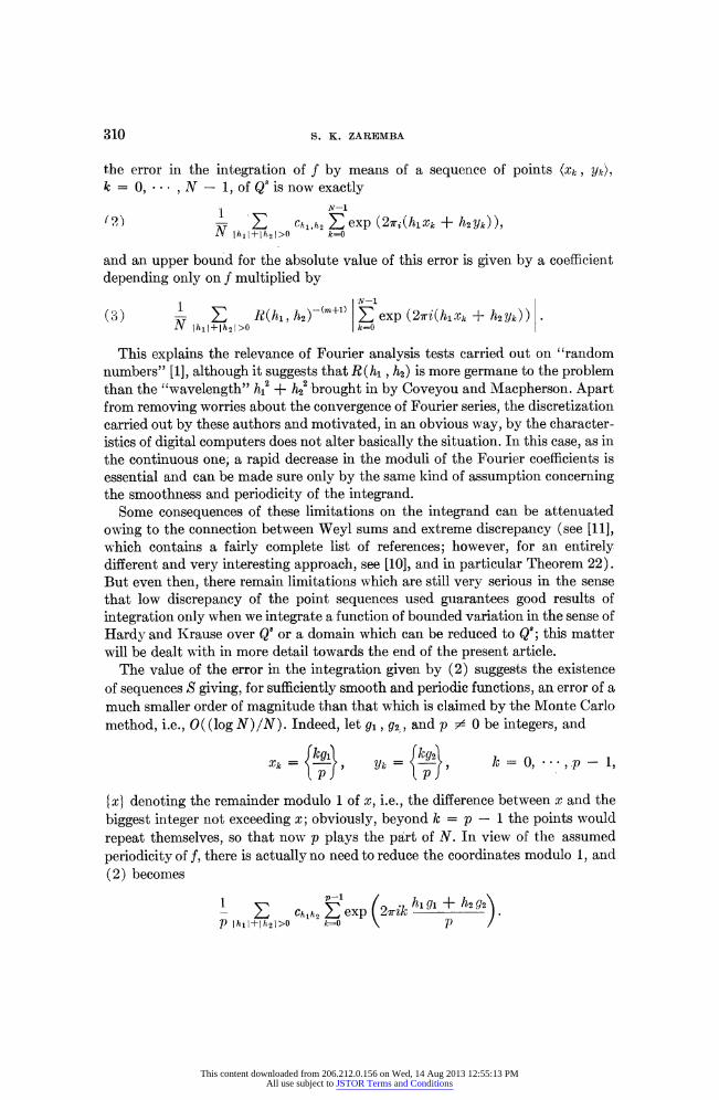
the error in the integration of f by means of a sequence of points (Xk, Yk),

k = 0,N** - 1, of Qs is now exactly

1 N-1 f ) ) - E Chj,h2 E exp (2,7ri (hxk + h2yk)), N lhll+lh21>? k=O

and an upper bound for the absolute value of this error is given by a coefficient depending only on f multiplied by

1 N-1

(3) - E R(h1, Ih2< (+ Z exp (2-nri(hlXk + h2Yk)) N hi I+Ih21 >0 k=O

This explains the relevance of Fourier analysis tests carried out on "random numbers" [1], although it suggests that R (hi , h2) is more germane to the problem than the "wavelength" hi2 + h22 brought in by Coveyou and Macpherson. Apart from removing worries about the convergence of Fourier series, the discretization carried out by these authors and motivated, in an obvious way, by the character- istics of digital computers does not alter basically the situation. In this case, as in the continuous one, a rapid decrease in the moduli of the Fourier coefficients is essential and can be made sure only by the saime kind of assumption concerning the smoothness and periodicity of the integrand.

Some consequences of these limitations on the integrand can be attenuated owing to the connection between Weyl sums and extreme discrepancy (see [11], which contains a fairly complete list of references; however, for an entirely different and very interesting approach, see [10], and in particular Theorem 22). But even then, there remain limitations which are still very serious in the sense that low discrepancy of the point sequences used guarantees good results of integration oinly when we integrate a function of bounded variation in the sense of Hardy and Krause over Q' or a domain which can be reduced to Q8; this matter will be dealt with in more detail towards the end of the present article.

The value of the error in the integration given by (2) suggests the existence of sequences S giving, for sufficiently smooth and periodi-c functions, an error of a much smaller order of magnitude than that which is claimed by the Monte Carlo method, i.e., O((log N)/N). Indeed, let gi, 92g, and p - 0 be integers, and

X k={g!, y =k2~} Xk ={, Y={ 2 k = O, .. * , p-1,

{x} denoting the remainder modulo 1 of x, i.e., the difference between x and the biggest integer not exceeding x; obviously, beyond k = p - 1 the points would repeat themselves, so that now p plays the part of N. In view of the assumed periodicity of f, there is actually no need to reduce the coordinates modulo 1, and (2) becomes

- E chjh2E exp 2heik w+h2 . p lhll+lh2l>0 k=O p



MNIONTE CARLO AND QUASI-MONTE CARLO METHODS 311

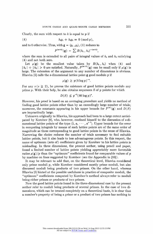
Clearly, the sum with respect to k is equal to p if

(4) h1ig + h2q2 0 (mod p),

and to 0 otherwise. Thus, with g = ( , g2), (3) reduces to

p()m+)(g) =

E R(hi, h2) ( X

where the sum is extended to all pairs of integral values of hi and h2 satisfying (4) and not both zero.

Let p(g) be the smallest value taken by R(hi, h2) when (4) and I h1 + h2 1 > 0 are satisfied. Naturally, p(m+l)(g) can be small only if p(g) is large. The extension of the argument to any number of dimensions is obvious. Hlawka [5] calls the s-dimensional lattice point g good modulo p if

p(g) > p(S log p)-

For any s (s ? 2), he proves the existence of good lattice points modulo any prime p. With their help, he also obtains sequences S of p points for which

D(S) ? p'(80 log p)8.

However, his proof is based on an averaging procedure and yields no method of finding good lattice points other than by an exceedingly large number of trials; moreover, the constants appearing in his upper bounds for p(n) (g) and D(S) are impractically large.

Unknown originally to Hlawka, his approach had been to a large extent antici- pated by Korobov [9], who, however, confined himself to the discussion of s-dimensional lattice points of the type (1, a, * , a '). Upper bounds for the error in computing integrals by means of such lattice points are of the same order of magnitude as those corresponding to good lattice points in the sense of Hlawka. Narrowing the choice reduces the number of trials necessary to find suitable lattice points, but it also leads to less advantageous points. In this, respect, the name of optimum (sets of) coefficients given by Korobov to his lattice points.is misleading. In three dimensions, the present author, using pencil and paper, found a limited number of lattice points yielding appreciably more favorable ratios p(g)/p than the "optimum" coefficients found for comparable values of p by machine on lines suggested by Korobov (see the Appendix in [10]).

It may be relevant to add that, on the theoretical level, Hlawka considered only prime moduli p, while Korobov considered mostly prime moduli, but also discussed moduli being products of two primes. On the, other hand, whereas Hlawka [5] hinted at the possible usefulness in practice of composite moduli, the "optimum" coefficients computed by Korobov's method always refer to moduli being either primes or products of two primes.

Now the good lattice points found in the three-dimensional case by the present author refer to moduli being products of several primes. In the case of two di- menisions, which can be treated completely on a theoretical basis, it is clear that a number's property of being a prime or a product of two primes has nothing to



312 S. K. ZAREMBA

do with its suitability as a modulus for good lattice points. In this case, there is a general recipe for optimizing lattice points in the sense of maximizing the ratio

P(g)/p. Korobov [10] noticed that with s = 2 one could obtain values of p(g) of the

order of magnitude of p instead of p(log p)-2, and that one could expect particularly satisfactory results when putting p = u,n , gi = 1, 92 = un_- , where (u,) is the sequence of Fibonacci numbers given by

Ul = U2 = 1) Un+2 = Un+1 + Un n = 1, 2, )

The present author [14], at that time still unaware of Korobov's work, showed that such lattice points yielded exactly p(g) = un-2 and that, apart from the trivial case of p = U4 = 3, this corresponded to the best possible ratio p(g)/p.

One finds, then, that

p(2) (g) < (256 log un + 60)un 2 n > 5,

and consequently, for any m > 2,

P(m (g) < (256log Un+ 60)u -2 , n > 5.

The assumption that the integrand should be periodic with a unit period in each variable appears at first sight to be a severe limitation. Korobov [10] suggested a method of reducing the general case to that of an integrand with the required properties of periodicity. His method is very simple to apply, but has the drawback of producing inordinately large values of the mixed partial derivatives of the integrand, on which the upper bound for the error of integration essentially depends; moreover, this feature of his method becomes rapidly accentuated as the number of dimensions increases. The present author [17] devised an alterna- tive method of replacing the integrand by a periodic function which is free of this inconvenience. The results of computing experiments, carried out mostly at the Mathematics Research Center, United States Army, University of Wisconsin and partly at the University College of Swansea, suggest that the method in question is likely to be more efficient than the conventional methods of computing double integrals.

Besides some bright promises, the use of good lattice points brought home a serious warning conceming Monte Carlo integration over domains which can be quite regular, but do not reduce to s-dimensional intervals or unions of finite numbers of such intervals. Assuming the domain to be bounded, one might think of reducing the integration over this domain to one over an s-dimensional interval by introducing a new function equal to the given one in the original domain of integration, and to 0 outside it. The difficulty which arises then is the following: However smooth the initially given function may be, the new one, in general, will not be of bounded variation in the sense of Hardy and Krause, not to mention the possibility of expanding it into a convergent multiple Fourier series. For such cases, Hlawka [4] established an upper bound for the error in the computation of the integral, which is of the order of D(S)lIs, and, therefore, for more than two dimensions, much bigger than that which is promised by the Monte Carlo method.




Now Hlawka's upper bound for the error cannot be substantially improved upon without drastic additional assumptions. Indeed, the set S of points of Q8 generated by a good lattice point is nothing else than the intersection of a certain lattice L with Q8, and, with a little geometry of numbers, it is not particularly difficult to prove the existence of an (s - 1)-dimensional linear variety H8-1 containing more than (4s)l-8pliI8 points of S [15]. Let, for instance, the integrand be equal to 1 everywhere, and the domain of integration be the part of Q8 situated on one side of an (s - 1) -dimensional linear variety Hf8-' parallel and arbitrarily close to H81. Depending on the side of Hs1- on which Hf8-' is situated, the points of S n H8'- will be contributing, or not contributing, to the computation of the integral, making a difference of more than (4s)l`8plI8 to the value obtained. Since the true values of the integral in the two cases are capable of differing arbitrarily little, it follows that at least in one of the two cases the error in the computation will exceed 1(4s)l-8pl18. Thus, apart from the power of log p which is missing now, this error will be of the order of magnitude of Hlawka's upper bound.

It follows that in the case of more than two dimensions, even a point sequence which passes stringent discrepancy tests can be quite unreliable as an instrument of Monte Carlo computations as soon as more general domains of integration than multidimensional intervals are allowed. This leads us to the following important question:

Are there arbitrarily long sequences S = (xo, * , XN-1) of points of Q8 having the property that, for any set A contained in Q8 and satisfying reasonable regu- larity conditions to be specified but allowing sets of a more general nature than s-dimensional intervals or finite unions thereof, and for any function f(x) with smoothness properties to be specified, the absolute error

Lf(x)dx- AT` >f(xi) xiEA

should have an upper bound of an order of magnitude appreciably better than pl11? Furthermore, if such sequences exist, one would like to have methods for constructing them, or, failing this, to have these sequences so characterized as to enable us to test them for the property in question. Assuming that such point sequences were used, this would provide, for the first time, a mathematically sound justification for the use of determinate sequences (as opposed to sequences obtained in the course of the computations by genuinely random devices) in the Monte Carlo computation of integrals over domains of a reasonably general class. However, this would be the case only if a sufficiently favorable upper bound for the error could be obtained, which is by no means certain.

REFERENCES

[1] R. R. COVEYOU AND R. D. MACPHERSON, Fourier analysis of uniform random number generators, J. Assoc. Comput. Mach., 14 (1967), pp. 100-119.

[2] S. FAEDO, Ordine di grandezza dei coefficienti di Eulero-Fourier delle funzioni di due variabili, Ann. Scuola Norm. Sup. Pisa (2), 6 (1937), pp. 225-246.

[3] J. HALTON AND S. K. ZAREMBA, Extreme and mean-square discrepancy, in preparation.



314 S. K. ZAREMBA

[4] E. HLAWKA, Funktionen von beschrdnkter Variation in der Theorie der Gleichverteilung, Ann. Mat. Pura Appl. 1 (4), 54 (1961), pp. 325-334.

[5] , Zur angendherten Berechnung mehrfacher Integrale, Monatsh. Math., 66 (1962), pp. 140-151.

[6] M. G. KENDALL AND B. BABINTON-SMITH, Randomness and random sampling numbers, J. Roy. Statist. Soc., 101 (1938), pp. 147-166.

[7] J. F. KOKSMA, A general theorem from the theory of uniform distribution modulo 1, Mathematica Zutphen B, 11 (1942), pp. 7-11. (In Dutch.)

[8] A. N. KOLMOGOROV, On tables of random numbers, Sankhya Ser. A, 25 (1963), pp. 369-376.

[9] N. -A. KOROBOV, The approximate computation of multiple integrals, Dokl. Akad. Nauk SSSR, 124 (1959), pp. 1207-1210.

[10] , Numbertheoretical Methods in Numerical Analysis, Fizmatgiz, Moscow, 1963. [11] W. J. LEVEQUE, An inequality connected with Weyl's criterion for uniform distribution,

Proc. Symposia Pure Math., vol. 8, American Mathematical Society, Provi- dence, 1965, pp. 22-30.

[12] K. F. ROTH, On irregularities of distribution, Mathematika, 1 (1954), pp. 73-79. [13] YU. A. SHREIDER, ed., The Monte Carlo Method. The Method of Statistical Trials, G. J. Tee,

transl., Pergamon Press, Oxford, 1966. [14] S. K. ZAREMBA, Good lattice points, discrepancy, and numerical integration, Ann. Miat.

Pura Appl. (4), 73 (1966), pp. 293-318. [15] , Good lattice points in the sense of Hlawka and Monte Carlo integration, Monatsh.

Math., 72 (1968), to appear. [16] , Some applications of multidimensional integration by parts, Ann. Polon. Math.,

21 (1968), to appear. [17] , A quasi-Monte Carlo Method for computing double and other multiple integrals,

in preparation.



the mathematical basis of monte carlo and quasi-monte carlo methods

Documents