the mathematica journal a study of super-nonlinear motion ... · a study of super-nonlinear motion...

The Mathematica® Journal

A Study of Super-Nonlinear Motion of a Simple PendulumHaiduke Sarafian

Two identically charged simple pendulums are allowed to swing in a vertical plane, acted upon by gravity and their mutual electrostatic interactive repulsive forces. We show that the inclusion of the electrostatic interaction makes the movement of the pendulums highly nonlinear. To describe the motion, we quantify the relevant time-dependent kinematic and dynamic quantities. Our analysis also includes an extended study of equal and oppositely charged pendulums. Motivated by the outcomes of the calculation, the author manufactured a real-life replica of the study demonstrating the features of the interactive pendulums; a photograph of the replica is included.

‡ Introduction and MotivationThe motion of a simple pendulum under the pull of gravity has been studied for ages.Most standard science and engineering texts have chapters devoted to the analysis of thisproblem. However, a thorough literature search reveals that the description of the motionof one such pendulum when perturbed by exotic forces is much less extensive. Amongmany feasible potential scenarios of perturbing the motion of a pendulum in a controlledand quantifiable manner is to cross-pollinate mechanics with electrostatics using a pair ofcharged pendulums. Based on the results of this analysis, one may argue that the answersto the “what-if” scenarios of this project would have remained unresolved before theadvent of the Mathematica era. This article uses the familiar laws of Newtonian mechanics and electrostatic interactions,as introduced to students in college science and engineering courses. Hence, the physicsof this article, its mathematical analysis, and the included Mathematica programs mightappeal to a wide range of readers.To simplify the analysis and to stress the important aspects of the physics of the project,we consider a symmetrical situation, with two identical pendulums.This is the problem: Consider two identical simple pendulums. Assume each pendulum iscomposed of a point-mass m, electric charge q, and string length {. Swing the pendulumssymmetrically about the vertical reference line that passes through their common pivotand hold them horizontal. Drop them simultaneously and let them swing under gravity.Then analyze the motion of each pendulum in terms of the parameters m, q, and {.

The Mathematica Journal 13 © 2011 Wolfram Media, Inc.

This is the problem: Consider two identical simple pendulums. Assume each pendulum iscomposed of a point-mass m, electric charge q, and string length {. Swing the pendulumssymmetrically about the vertical reference line that passes through their common pivotand hold them horizontal. Drop them simultaneously and let them swing under gravity.Then analyze the motion of each pendulum in terms of the parameters m, q, and {.

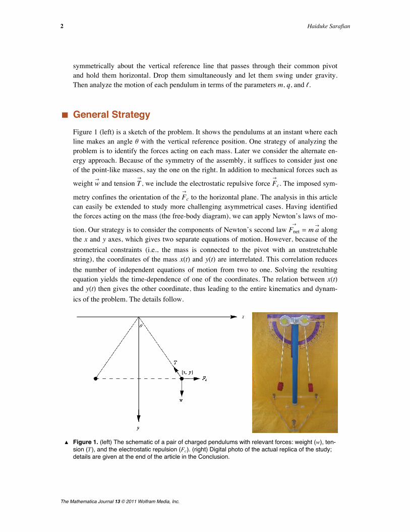
‡ General StrategyFigure 1 (left) is a sketch of the problem. It shows the pendulums at an instant where eachline makes an angle q with the vertical reference position. One strategy of analyzing theproblem is to identify the forces acting on each mass. Later we consider the alternate en-ergy approach. Because of the symmetry of the assembly, it suffices to consider just oneof the point-like masses, say the one on the right. In addition to mechanical forces such as

weight wØ

and tension TØ

, we include the electrostatic repulsive force FØ

c. The imposed sym-

metry confines the orientation of the FØ

c to the horizontal plane. The analysis in this articlecan easily be extended to study more challenging asymmetrical cases. Having identifiedthe forces acting on the mass (the free-body diagram), we can apply Newton’s laws of mo-

tion. Our strategy is to consider the components of Newton’s second law FnetØ

= m aØ

alongthe x and y axes, which gives two separate equations of motion. However, because of thegeometrical constraints (i.e., the mass is connected to the pivot with an unstretchablestring), the coordinates of the mass xHtL and yHtL are interrelated. This correlation reducesthe number of independent equations of motion from two to one. Solving the resultingequation yields the time-dependence of one of the coordinates. The relation between xHtLand yHtL then gives the other coordinate, thus leading to the entire kinematics and dynam-ics of the problem. The details follow.

Ú Figure 1. (left) The schematic of a pair of charged pendulums with relevant forces: weight (w), ten-sion (T), and the electrostatic repulsion (Fc). (right) Digital photo of the actual replica of the study; details are given at the end of the article in the Conclusion.

2 Haiduke Sarafian


‡ Analysis

We begin with Newton’s second law, FnetØ

= m aØ

. Because of the planar motion of themass, we project this equation along the horizontal and vertical directions. This gives

HFnetLxØ

= m axØ

and HFnetLyØ

= m ayØ

. There are advantages to confining the motion of themass within the first quadrant; we select the downward direction as the positive y axis.These two equations yield

(1)Fc - T sin q = m x..,

(2)m g- T cos q = m y..,

where g is the acceleration of gravity, T is the tension in the line, and Fc =k q2

4 x2 is the elec-

trostatic force, with q being the charge and x the horizontal coordinate of the mass. The ac-celerations of the mass along the x and y axes are x

.. and y

... According to standard notation,

x° ª ddt x, and so on. We rearrange these equations and find their ratio:

(3)T sin q

T cos q=

Fc -m x..

m g-m y.. .

Since, according to Figure 1, tan q = xy , equation (3) yields

(4)g- y..=

y

x

Fc

m- x..

.

Because the length of the string is constant, we write x2 + y2 = {2, which gives

y = + {2 - x2 . Differentiating the latter twice with respect to time yields

(5)-y..= Bx x

..+ x° 2 + Hx x° L2 I{2 - x2M-1F I{2 - x2M-

12 .

Substituting equation (5) into equation (4) and simplifying the result gives

(6){2 x2 x..+

x3 {2

{2 - x2x° 2 + g x3 {2 - x2 -

k q2

4 mI{2 - x2M = 0.

A Study of Super-Nonlinear Motion of a Simple Pendulum 3


Define a dimensionless variable x = x{ , which gives x

°= x°

{ and x..= x

..

{ . Substituting theseinto equation (6) yields

(7)x2 x..+

x3

1- x2x° 2+ a x3 1- x2 - b I1- x2M = 0,

where the two auxiliary constant parameters are a =g{ and b =

k q2

4m {3 . The parameter a ispurely mechanical while b is influenced by both mechanics and electrostatics. Forpendulums charged with equal and opposite charges and those with no charge, the counterequations of equation (7) are, respectively,

(8)x2 x..+

x3

1- x2x° 2+ a x3 1- x2 + b I1- x2M = 0,

(9)x..+

x

1- x2x° 2+ a x 1- x2 = 0.

Equations (7), (8), and (9) are second-order and highly nonlinear differential equations.For a set of chosen practical values of a and b we apply DSolve; Mathematica fails toproduce symbolic solutions. We then apply NDSolve along with the relevant initialconditions, namely, xHt = 0L = { and x° Ht = 0L = 0. The solutions are shown in Figure 2.

values = 9{ Ø 1.0, m Ø 5 µ 10-3, q Ø 2 µ 10-6, k Ø 9 µ 109, g Ø 9.8=;

8a, b< = :g

{,

k q2

4 m {3> ê. values

89.8, 1.8<

eqns@n_D :=

x@tD2 x''@tD +x@tD3

1 - x@tD2x'@tD2 + a x@tD3 1 - x@tD2 +

n b I1 - x@tD2M ê. values

soleqns =

TableANDSolveA9eqns@nD ã 0, xA1 µ 10-8E ã NA1 - 10-7, 10E,

x'A1 µ 10-8E ã 0=, x@tD,

9t, 1 µ 10-6, If@n ã -1, 3.0, If@n ã 0, 0.6, 0.55DD=E,

8n, -1, 1<E;

4 Haiduke Sarafian


ShowATableAPlotAEvaluate@x@tD ê. soleqnsPmTD,

9t, 1 µ 10-6, If@m ã 1, 3.0, 0.6D=, AxesLabel Ø 8t, "x"<,

PlotStyle Ø [email protected], [email protected] mD,If@m ã 1, Dashing@81, 0.0001<D,[email protected], 0.001< mDD<,

PlotRange Ø 8Automatic, 80, 1<<E, 8m, 1, 3<EE

0.0 0.5 1.0 1.5 2.0 2.5 3.0t

0.2

0.4

0.6

0.8

1.0x

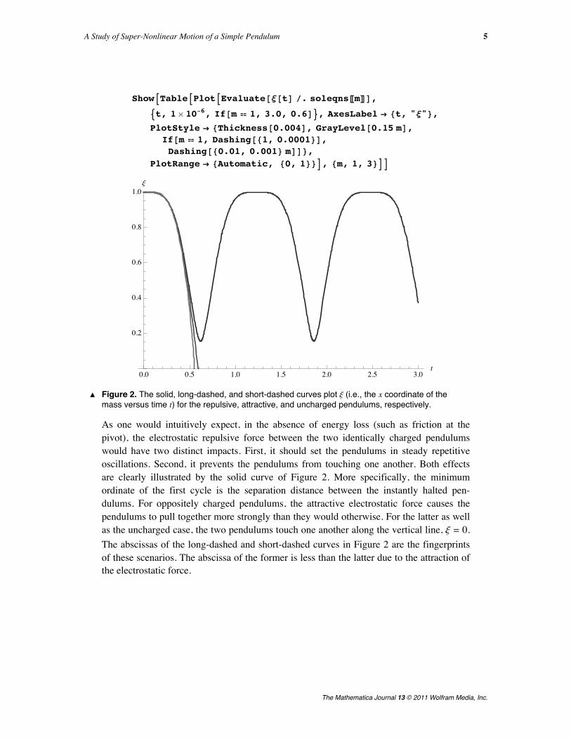
Ú Figure 2. The solid, long-dashed, and short-dashed curves plot x (i.e., the x coordinate of the mass versus time t) for the repulsive, attractive, and uncharged pendulums, respectively.

As one would intuitively expect, in the absence of energy loss (such as friction at thepivot), the electrostatic repulsive force between the two identically charged pendulumswould have two distinct impacts. First, it should set the pendulums in steady repetitiveoscillations. Second, it prevents the pendulums from touching one another. Both effectsare clearly illustrated by the solid curve of Figure 2. More specifically, the minimumordinate of the first cycle is the separation distance between the instantly halted pen-dulums. For oppositely charged pendulums, the attractive electrostatic force causes thependulums to pull together more strongly than they would otherwise. For the latter as wellas the uncharged case, the two pendulums touch one another along the vertical line, x = 0.The abscissas of the long-dashed and short-dashed curves in Figure 2 are the fingerprintsof these scenarios. The abscissa of the former is less than the latter due to the attraction ofthe electrostatic force.



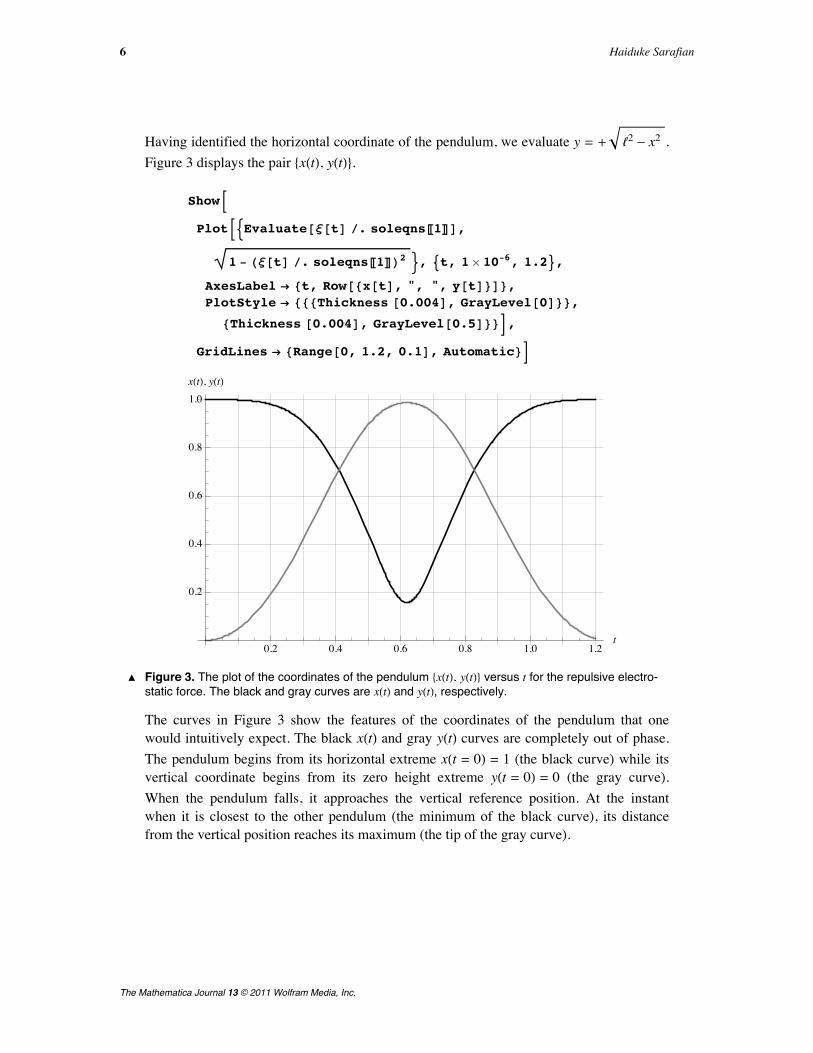
Having identified the horizontal coordinate of the pendulum, we evaluate y = + {2 - x2 .Figure 3 displays the pair 8xHtL, yHtL<.

ShowB

PlotB:Evaluate@x@tD ê. soleqnsP1TD,

1 - Hx@tD ê. soleqnsP1TL2 >, 9t, 1 µ 10-6, 1.2=,

AxesLabel Ø 8t, Row@8x@tD, ", ", y@tD<D<,PlotStyle Ø 888Thickness @0.004D, GrayLevel@0D<<,

8Thickness @0.004D, [email protected]<<F,

GridLines Ø 8Range@0, 1.2, 0.1D, Automatic<F

0.2 0.4 0.6 0.8 1.0 1.2t

0.2

0.4

0.6

0.8

1.0xHtL, yHtL

Ú Figure 3. The plot of the coordinates of the pendulum 8xHtL, yHtL< versus t for the repulsive electro-static force. The black and gray curves are xHtL and yHtL, respectively.

The curves in Figure 3 show the features of the coordinates of the pendulum that onewould intuitively expect. The black xHtL and gray yHtL curves are completely out of phase.The pendulum begins from its horizontal extreme xHt = 0L = 1 (the black curve) while itsvertical coordinate begins from its zero height extreme yHt = 0L = 0 (the gray curve).When the pendulum falls, it approaches the vertical reference position. At the instantwhen it is closest to the other pendulum (the minimum of the black curve), its distancefrom the vertical position reaches its maximum (the tip of the gray curve).

6 Haiduke Sarafian


To confirm that our computation sets the pendulum in a circular path, we applyParametricPlot to graph its traversed path.

ParametricPlotB

FlattenB:Evaluate@x@tD ê. soleqnsP1TD,

EvaluateB- 1 - Hx@tD ê. soleqnsP1TL2 F>F, 9t, 1 µ 10-6, 0.8=,

AxesLabel Ø 8x@mD, y@mD<, PlotRange Ø 880, 1<, 80, -1.0<<,GridLines Ø Automatic,PlotStyle Ø [email protected], GrayLevel@0D<,

ImageSize Ø 250F

0.2 0.4 0.6 0.8 1.0xHmL

-1.0

-0.8

-0.6

-0.4

-0.2

0.0yHmL

Ú Figure 4. The circular path traversed by the pendulum.

Note that 8xHtL, yHtL< are given numerically, not analytically. Even so, Mathematica lets usevaluate the time derivatives related to kinematic quantities, such as 9x° HtL, x

..HtL= and

9y° HtL, y..HtL=. We display these in Figure 5.

8xcoordinate, xspeed, xacc< =Table@D@x@tD ê. soleqnsP1T, 8t, n<D, 8n, 0, 2<D;

8ycoordinate, yspeed, yacc< =

TableBDB 1 - Hx@tD ê. soleqnsP1TL2 , 8t, n<F, 8n, 0, 2<F;



ColumnB::

PlotB8xcoordinate, 0.5 xspeed, 0.03 xacc<, 8t, 0.001, 3.0<,

PlotStyle Ø [email protected], GrayLevel@0D<,8Thickness @0.004D, GrayLevel@0D, [email protected]<D<,[email protected], GrayLevel@0D, [email protected]<D<<,

AxesLabel Ø :t, RowB:x, ", ", x°, ", ", x".."

>F>,

PlotRange Ø All, ImageSize Ø 275F,

PlotB8ycoordinate, 0.5 yspeed, 0.08 yacc<, 8t, 0.01, 1.2<,

PlotStyle Ø [email protected], GrayLevel@0D<,8Thickness @0.004D, GrayLevel@0D, [email protected]<D<,[email protected], GrayLevel@0D, [email protected]<D<<,

AxesLabel Ø :t, RowB:y, ", ", y°, ", ", y".."

>F>,

PlotRange Ø All, ImageSize Ø 275F>>F

:

0.5 1.0 1.5 2.0 2.5 3.0t

-1.5

-1.0

-0.5

0.5

1.0

1.5

2.0

x, x° , x..

,

0.2 0.4 0.6 0.8 1.0 1.2t

-1.0

-0.5

0.5

1.0

y, y° , y..

>

Ú Figure 5. In both graphs, the solid, short-dashed, and long-dashed curves correspond to position coordinates and their associated speed and acceleration, respectively. For the sake of clarity, in the left graph x° and x.. are scaled down by a factor of 0.5 and 0.03, respectively. In the right graph, y° and y.. are scaled down by a factor of 0.5 and 0.08, respectively.

Graphically speaking, speed is the slope of the position with respect to time; accelerationis the slope of the speed with respect to time. A close inspection of the depicted plotsunderlines the graphical interrelationships of the corresponding quantities. The authorspeculates the “noise” in the y

..HtL signal (the long-dashed curve) originated from the

second-order numerical derivative procedure. The double-hump of y..HtL would have re-

mained undetected had it not been depicted graphically.

8 Haiduke Sarafian


Graphically speaking, speed is the slope of the position with respect to time; accelerationis the slope of the speed with respect to time. A close inspection of the depicted plotsunderlines the graphical interrelationships of the corresponding quantities. The authorspeculates the “noise” in the y

..HtL signal (the long-dashed curve) originated from the

second-order numerical derivative procedure. The double-hump of y..HtL would have re-

mained undetected had it not been depicted graphically.

‡ An Alternative Approach Using Polar CoordinatesSince each individual mass swings along a circular path, this suggests that the problemmight be more efficiently analyzed in polar coordinates.

Earlier, we introduced a dimensionless variable x = x{ . According to Figure 1, x = sin q.

We then evaluate x.= q

°cos q and x

..= q..

cos q - q° 2

sin q. Substituting these into equation (7)and simplifying yields the equation of motion in the polar coordinate system,

(10)q..+ a sin q - b

cos q

sin2 q= 0.

Replacing b by -b or 0 results in counterparts of equations (8) and (9), respectively. Inthe absence of electric charge, b = 0 and equation (10) describes the motion of anuncharged simple pendulum. For small angles, sin q > q and the corresponding linearizedequation assumes a textbook form: q

..+

g{ q = 0. For a charged pendulum b ¹≠ 0 and, irre-

spective of the oscillation amplitude, equation (10) describes the motion of a highly super-nonlinear pendulum. As in the previous section, applying DSolve fails to generatesymbolic output, so again we use the same set of initial conditions and solve the equationnumerically. The solution of the equation of motion in the polar coordinate system shouldmatch the Cartesian results. As shown in Figure 6, the agreement is perfect.

eqnsq@n_D := q''@tD + a Sin@q@tDD + n bCos@q@tDD

Sin@q@tDD2

soleqnsq =

TableBNDSolveB:eqnsq@nD ã 0, qA1 µ 10-8E ãp

2,

q'A1 µ 10-8E ã 0>, q@tD, 9t, 1 µ 10-8, 3.0=F, 8n, -1, 0<F;



ShowBPlotB:180

pEvaluate@q@tD ê. soleqnsqP1TD,

180

pEvaluateBArcTanB

x@tD ê. soleqnsP1T

1 - Hx@tD ê. soleqnsP1TL2FF>,

9t, 1 µ 10-8, 3.0=, AxesLabel Ø 8t, Row@8q, " HdegL"<D<,

PlotStyle Ø [email protected], [email protected]<,[email protected], GrayLevel@0D<<<,

PlotRange Ø 8Automatic, 80, 90<<FF

0.0 0.5 1.0 1.5 2.0 2.5 3.0t

20

40

60

80

q HdegL

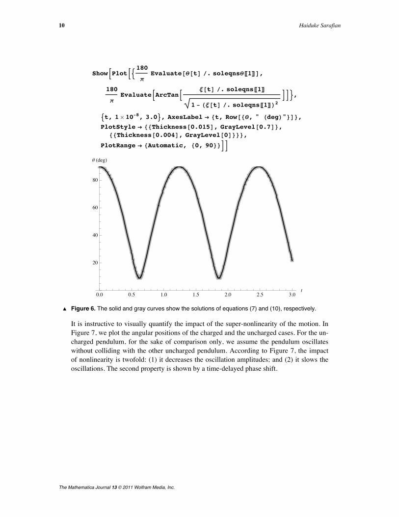
Ú Figure 6. The solid and gray curves show the solutions of equations (7) and (10), respectively.

It is instructive to visually quantify the impact of the super-nonlinearity of the motion. InFigure 7, we plot the angular positions of the charged and the uncharged cases. For the un-charged pendulum, for the sake of comparison only, we assume the pendulum oscillateswithout colliding with the other uncharged pendulum. According to Figure 7, the impactof nonlinearity is twofold: (1) it decreases the oscillation amplitudes; and (2) it slows theoscillations. The second property is shown by a time-delayed phase shift.

10 Haiduke Sarafian


ShowBPlotB:180

pEvaluate@q@tD ê. soleqnsqP2TD,

180

pEvaluateBArcTanB

x@tD ê. soleqnsP1T

1 - Hx@tD ê. soleqnsP1TL2FF>,

9t, 1 µ 10-8, 3.0=, AxesLabel Ø 8t, Row@8q, " HdegL"<D<,

PlotStyle Ø [email protected], [email protected]<,[email protected], GrayLevel@0D<<<,

PlotRange Ø 8Automatic, 8-90, 90<<FF

0.5 1.0 1.5 2.0 2.5 3.0t

-50

50

q HdegL

Ú Figure 7. The black and gray curves represent the angular positions of the charged and un-charged pendulums, respectively.

Knowing the value of qHtL, we evaluate related physical quantities such as the angularspeed w ª q

°HtL and angular acceleration a ª q

..HtL. Here again we emphasize the usefulness

of Mathematica: it enables us to differentiate a nonanalytic function. Figure 8 displays the:qHtL, q

°HtL, q

..HtL> for b ¹≠ 0.

repulsive = 8qcoordinate, qspeed, qacc< =Table@D@q@tD ê. soleqnsqP1T, 8t, n<D, 8n, 0, 2<D;



PlotB:180

pqcoordinate,

180

p0.4 qspeed,

180

p0.02 qacc>,

8t, 0.001, 3.0<,PlotStyle Ø [email protected], GrayLevel@0D<,

[email protected], GrayLevel@0D, [email protected]<D<,[email protected], GrayLevel@0D, [email protected]<D<<,

AxesLabel Ø :t, RowB:q, ", ", q°, ", ", q

"..">F>,

PlotRange Ø AllF

0.5 1.0 1.5 2.0 2.5 3.0t

-50

50

q, q°, q..

Ú Figure 8. The solid, short-dashed, and long-dashed curves correspond to qHtL, q°HtL, and q

..HtL for

b ¹≠ 0, respectively.

As we mentioned in the previous section, graphically, the angular speed and the angular ac-celeration are to be interpreted as the slope of the angular position with respect to timeand the slope of the angular speed with respect to time, respectively. The short-dashed andlong-dashed curves depicted in Figure 8 agree with these interpretations.

‡ Phase Diagrams

In the section Analysis, we evaluated a set of kinematic quantities such as qHtL, q°HtL, and

q..HtL to describe the oscillations of the masses. Now, by suppressing the time variable, t,

we apply ParametricPlot and graph subsets of these quantities, namely 9q, q°=, :q, q

..>,

:q°, q..>, and :q, q

°, q..>. We also display the same sets for the uncharged pendulums. These

are all shown in Figure 9.

12 Haiduke Sarafian


neutral = 8qcoordinate, qspeed, qacc< =Table@D@q@tD ê. soleqnsqP2T, 8t, n<D, 8n, 0, 2<D;

s12 =ShowA9ParametricPlotAFlatten@8neutralP1T, neutralP2T<D,

9t, 1 µ 10-8, 3=,

PlotStyle Ø [email protected], GrayLevel@0D<E,

ParametricPlotAFlatten@8repulsiveP1T, repulsiveP2T<D,

9t, 1 µ 10-8, 3=,

PlotStyle Ø [email protected], GrayLevel@0D,[email protected]<D<E=, ImageSize Ø 250,

AxesLabel Ø 9q, q°=, AspectRatio Ø 1E;

s13 =

ShowB9ParametricPlotAFlatten@8neutralP1T, neutralP3T<D,

9t, 1 µ 10-8, 3=,


ParametricPlotAFlatten@8repulsiveP1T, repulsiveP3T<D,

9t, 1 µ 10-8, 3=,

PlotStyle Ø [email protected], GrayLevel@0D,[email protected]<D<E=, ImageSize Ø 250, PlotRange Ø All,

AxesLabel Ø :q, q".."

>, AspectRatio Ø 1F;

s23 =

ShowB9ParametricPlotAFlatten@8neutralP2T, neutralP3T<D,

9t, 1 µ 10-8, 3=,


ParametricPlotA

Flatten@8repulsiveP2T, 0.4 repulsiveP3T<D,9t, 1 µ 10-8, 3=,


AxesLabel Ø :q°, q

"..">, AspectRatio Ø 1F;



s3D123 =

ShowB

9ParametricPlot3DA

Flatten@8neutralP1T, neutralP2T, 0.4 neutralP3T<D,9t, 1 µ 10-8, 3=,


ParametricPlot3DA

Flatten@8repulsiveP1T, repulsiveP2T, 0.4 repulsiveP3T<D,9t, 1 µ 10-8, 3=,


AxesLabel Ø :q, q°, q

"..">, AspectRatio Ø 1, BoxRatios Ø 1F;

Show@GraphicsGrid@88s12, s13<, 8s23, s3D123<<D,ImageSize Ø 350D

-1.5 -1.0 -0.5 0.5 1.0 1.5q

-4

-2

2

4

q°

-1.5 -1.0 -0.5 0.5 1.0 1.5q

20

40

60

q..

-4 -2 2 4 q°

-10

-5

5

10

15

20

25

q..

-10

1q

-4-2

024

q°

0

10

20

q..

Ú Figure 9. The solid and the dashed curves are the “phase diagrams” of the uncharged and the charged pendulums, respectively.

With the exception of the top-left graph, a traditional phase diagram, the other three dia-grams have seldom, if ever, been discussed in literature. These three graphs are examplesdemonstrating how Mathematica can be deployed to explore fresh ideas. Their descriptiveinterpretations are explicit; they are useful graphs assisting our understanding of thephysics of the problem. One of the objectives of this article is to demonstrate the impactof the electrostatic interactions of the charged pendulums on the oscillations of themasses. The two scenarios are distinguished from one another by the presence of electriccharge. Hence, to avoid the auxiliary potential side effects, such as mechanical collisionsof the uncharged masses, we assume the uncharged pendulums pass through each otherwhen they meet. Therefore, the solid curve in the top-left plot of Figure 9 is symmetricallyextended to the q < 0 domain. The charged and the uncharged pendulums begin from thesame horizontal position, q = p ê 2. Their respective angular position q and the angularspeed q

° change accordingly. Beyond q = p ê 2, the super-nonlinearity of the oscillations

causes these two curves to diverge. In addition, the abscissa of the dashed curve is thesmallest separation angle of the charged pendulums.

14 Haiduke Sarafian


With the exception of the top-left graph, a traditional phase diagram, the other three dia-grams have seldom, if ever, been discussed in literature. These three graphs are examplesdemonstrating how Mathematica can be deployed to explore fresh ideas. Their descriptiveinterpretations are explicit; they are useful graphs assisting our understanding of thephysics of the problem. One of the objectives of this article is to demonstrate the impactof the electrostatic interactions of the charged pendulums on the oscillations of themasses. The two scenarios are distinguished from one another by the presence of electriccharge. Hence, to avoid the auxiliary potential side effects, such as mechanical collisionsof the uncharged masses, we assume the uncharged pendulums pass through each otherwhen they meet. Therefore, the solid curve in the top-left plot of Figure 9 is symmetricallyextended to the q < 0 domain. The charged and the uncharged pendulums begin from thesame horizontal position, q = p ê 2. Their respective angular position q and the angularspeed q

° change accordingly. Beyond q = p ê 2, the super-nonlinearity of the oscillations

causes these two curves to diverge. In addition, the abscissa of the dashed curve is thesmallest separation angle of the charged pendulums.

‡ ConclusionThe analysis of the characteristics of perturbed motion of a simple pendulum as presentedin this article illustrates the features of nonlinear dynamics and its interface withmechanics and electrostatics. The author’s extensive search of the literature indicated thatthis analysis is new. The proposed project accomplishes several instructional and research-oriented objectives. The author applied the basic principles of mechanics that are beingtaught in introductory physics and engineering courses and laid the foundation one step ata time to develop the equations describing the physics of the problem. A quick review ofthe article will convince the reader that the concept of the project is not hard to grasp;however, its detailed analysis leading to a quantifiable understanding hinges upon thesolutions of the challenging equations of motion. Without Mathematica’s powerful andflexible tools, such as NDSolve, as well as its numerical and especially its graphicsutilities, the analysis of this project, the super-nonlinear motion of the pendulum, mighthave remained unnoticed.Throughout the article, with its analysis and the accompanying Mathematica programs,the author encourages the reader to examine features of extended challenging scenarios.The article thus suggests a road map for explorations of problems in physics and extendsthe scope of the current status of nonlinear dynamics. For instance, in most texts thenonlinear motion of a simple pendulum is limited to the analysis of “the large amplitudeoscillations” of an uncharged, mechanical pendulum. This article extends consideration toadditional nonmechanical perturbation forces.

To make the project as comprehensive as possible, the author built a real-life replica ofthe study. For practical reasons, two 0.4 caliber cylindrical neodymium magnets are usedto mimic the effects of the electrostatic repulsive forces; a digital photo of the replica is in-cluded in Figure 1 (right).



To make the project as comprehensive as possible, the author built a real-life replica ofthe study. For practical reasons, two 0.4 caliber cylindrical neodymium magnets are usedto mimic the effects of the electrostatic repulsive forces; a digital photo of the replica is in-cluded in Figure 1 (right).

‡ Reference[1] S. Thornton and J. Marion, “Classical Dynamics of Particles and Systems,” 5th ed., Belmont,

CA: Brooks/Cole, 2003.

H. Sarafian, “A Study of Super-Nonlinear Motion of a Simple Pendulum,” The Mathematica Journal, 2011. dx.doi.org/doi:10.3888/tmj.13–14.

About the Author

Haiduke Sarafian is the John T. and Paige S. Smith Professor of Science at the Pennsylva-nia State University at the York campus of the University College. He received his Ph.D.in theoretical nuclear physics from Michigan State University in 1983. In 1999 he wasa Mathematica Visiting Scholar. He is also an independent Mathematica trainer(www.wolfram.com/services/training/sarafian.html).Haiduke SarafianThe Pennsylvania State UniversityUniversity CollegeYork, PA [email protected]

16 Haiduke Sarafian


the mathematica journal a study of super-nonlinear motion ... · a study of super-nonlinear motion...

Documents