The Markov Chain Monte Carlo Approach to

Importance Sampling in Stochastic Programming

by

Berk Ustun

B.S., Operations Research, University of California, Berkeley (2009)B.A., Economics, University of California, Berkeley (2009)

Submitted to the School of Engineeringin partial fulfillment of the requirements for the degree of

Master of Science in Computation for Design and Optimization

at the

MASSACHUSETTS INSTITUTE OF TECHNOLOGY

September 2012

c© Massachusetts Institute of Technology 2012. All rights reserved.

Author . . . . . . . . . . . . . . . . . . . . . . . . . . . . . . . . . . . . . . . . . . . . . . . . . . . . . . . . . . . . . . . . . . . .School of Engineering

August 10, 2012

Certified by . . . . . . . . . . . . . . . . . . . . . . . . . . . . . . . . . . . . . . . . . . . . . . . . . . . . . . . . . . . . . . .Mort Webster

Assistant Professor of Engineering SystemsThesis Supervisor

Certified by . . . . . . . . . . . . . . . . . . . . . . . . . . . . . . . . . . . . . . . . . . . . . . . . . . . . . . . . . . . . . . .Youssef Marzouk

Class of 1942 Associate Professor of Aeronautics and AstronauticsThesis Reader

Accepted by . . . . . . . . . . . . . . . . . . . . . . . . . . . . . . . . . . . . . . . . . . . . . . . . . . . . . . . . . . . . . . .Nicolas Hadjiconstantinou

Associate Professor of Mechanical EngineeringDirector, Computation for Design and Optimization

2

The Markov Chain Monte Carlo Approach to Importance

Sampling in Stochastic Programming

by

Berk Ustun

Submitted to the School of Engineeringon August 10, 2012, in partial fulfillment of the

requirements for the degree ofMaster of Science in Computation for Design and Optimization

Abstract

Stochastic programming models are large-scale optimization problems that are used to fa-cilitate decision-making under uncertainty. Optimization algorithms for such problems needto evaluate the expected future costs of current decisions, often referred to as the recoursefunction. In practice, this calculation is computationally difficult as it involves the evaluationof a multidimensional integral whose integrand is an optimization problem. Accordingly, therecourse function is estimated using quadrature rules or Monte Carlo methods. AlthoughMonte Carlo methods present numerous computational benefits over quadrature rules, theyrequire a large number of samples to produce accurate results when they are embedded inan optimization algorithm. We present an importance sampling framework for multistagestochastic programming that can produce accurate estimates of the recourse function using afixed number of samples. Our framework uses Markov Chain Monte Carlo and Kernel Den-sity Estimation algorithms to create a non-parametric importance sampling distribution thatcan form lower variance estimates of the recourse function. We demonstrate the increasedaccuracy and efficiency of our approach using numerical experiments in which we solve vari-ants of the Newsvendor problem. Our results show that even a simple implementation ofour framework produces highly accurate estimates of the optimal solution and optimal costfor stochastic programming models, especially those with increased variance, multimodal orrare-event distributions.

Thesis Supervisor: Mort WebsterTitle: Assistant Professor of Engineering Systems

3

Acknowledgments

I would like to take this opportunity to thank my advisors, Mort Webster and Panos Parpas,

who have supervised and funded my research at MIT over the past two years. This thesis

would not have been possible without their guidance, insight and patience. I would also like

to thank Youssef Marzouk, who helped develop and formalize many of the findings that I

present in this thesis, as well Bryan Palmintier, who frequently helped resolve all kinds of

important problems that I encountered in my research.

Much of this work has involved coding, debugging, computing and waiting... This process

was incredibly frustrating at times, but it has certainly been easier in my case thanks to Jeff

and Greg who manage the Svante cluster, as well as the anonymous users who post on the

CPLEX forums and the StackExchange network. I very much appreciate the fact that these

individuals have sacrificed their time and energy to solve problems that, quite frankly, did

not affect them in any way. I look forward to the day that I can help others as selflessly as

they have helped me.

Looking back at these past two years at MIT, I believe that I have been very fortunate

to have been admitted to the CDO program, but even more fortunate to have Laura Koller

and Barbara Lechner as my academic administrators. Their support has been invaluable,

and I cannot fathom how I could have completed this degree without them.

4

Contents

1 Introduction 13

2 Background 17

2.1 Modeling Decision-Making Problems using SP . . . . . . . . . . . . . . . . . 18

2.2 Solving SP Models with Decomposition Algorithms . . . . . . . . . . . . . . 19

2.2.1 Representing Expected Future Costs with the Recourse Function . . . 19

2.2.2 Approximating the Recourse Function with Cutting Planes . . . . . . 20

2.2.3 Stopping Procedures . . . . . . . . . . . . . . . . . . . . . . . . . . . 21

2.2.4 Overview of Decomposition Algorithms . . . . . . . . . . . . . . . . . 22

2.3 Using Monte Carlo Methods in Decomposition Algorithms . . . . . . . . . . 23

2.4 The Impact of Sampling Error in Decomposition Algorithms . . . . . . . . . 24

2.5 Reducing Sampling Error through Variance Reduction . . . . . . . . . . . . 26

2.5.1 Stratified Sampling . . . . . . . . . . . . . . . . . . . . . . . . . . . . 27

2.5.2 Quasi-Monte Carlo . . . . . . . . . . . . . . . . . . . . . . . . . . . . 27

2.5.3 Importance Sampling . . . . . . . . . . . . . . . . . . . . . . . . . . . 28

2.5.4 IDG Importance Sampling . . . . . . . . . . . . . . . . . . . . . . . . 30

3 The Markov Chain Monte Carlo Approach to Importance Sampling 33

3.1 Foundations of the Markov Chain Monte Carlo Approach to Importance Sam-

pling . . . . . . . . . . . . . . . . . . . . . . . . . . . . . . . . . . . . . . . . 34

3.1.1 The Zero-Variance Distribution . . . . . . . . . . . . . . . . . . . . . 34

3.1.2 Overview of MCMC Algorithms . . . . . . . . . . . . . . . . . . . . . 35

3.1.3 Overview of KDE Algorithms . . . . . . . . . . . . . . . . . . . . . . 36

5

3.2 The Markov Chain Monte Carlo Approach to Importance Sampling . . . . . 37

3.3 MCMC-IS in Practice . . . . . . . . . . . . . . . . . . . . . . . . . . . . . . . 40

3.4 MCMC-IS in Theory . . . . . . . . . . . . . . . . . . . . . . . . . . . . . . . 43

4 Numerical Experiments on Sampling Properties 45

4.1 The Newsvendor Model . . . . . . . . . . . . . . . . . . . . . . . . . . . . . . 46

4.1.1 A Simple Two-Stage Model . . . . . . . . . . . . . . . . . . . . . . . 46

4.1.2 A Multidimensional Extension . . . . . . . . . . . . . . . . . . . . . . 46

4.1.3 A Multistage Extension . . . . . . . . . . . . . . . . . . . . . . . . . 47

4.2 Experimental Setup . . . . . . . . . . . . . . . . . . . . . . . . . . . . . . . . 48

4.2.1 Experimental Statistics . . . . . . . . . . . . . . . . . . . . . . . . . . 48

4.2.2 Implementation . . . . . . . . . . . . . . . . . . . . . . . . . . . . . . 48

4.3 Sampling from the Important Regions . . . . . . . . . . . . . . . . . . . . . . 49

4.4 The Required Number of MCMC Samples . . . . . . . . . . . . . . . . . . . 52

4.4.1 The Curse of Dimensionality . . . . . . . . . . . . . . . . . . . . . . . 53

4.5 The Acceptance Rate of the MCMC Algorithm . . . . . . . . . . . . . . . . 55

4.6 Sampling from Bounded Regions . . . . . . . . . . . . . . . . . . . . . . . . 58

4.7 Choosing Kernel Functions and Bandwidth Estimators in the KDE Algorithm 62

4.8 Comparison to Existing Variance Reduction Techniques . . . . . . . . . . . . 63

4.8.1 Comparison to IDG Importance Sampling . . . . . . . . . . . . . . . 63

4.8.2 Comparison to Other Variance Reduction Techniques . . . . . . . . . 66

5 Numerical Experiments on Performance in Decomposition Algorithms 69

5.1 Experimental Setup . . . . . . . . . . . . . . . . . . . . . . . . . . . . . . . . 70

5.1.1 Experimental Statistics . . . . . . . . . . . . . . . . . . . . . . . . . . 70

5.1.2 Implementation . . . . . . . . . . . . . . . . . . . . . . . . . . . . . . 71

5.2 Impact of MCMC-IS Estimates in a Decomposition Algorithm . . . . . . . . 72

5.3 Impact of MCMC-IS Estimates in Stopping Tests . . . . . . . . . . . . . . . 74

5.4 Computational Performance of MCMC-IS in Multistage SP . . . . . . . . . . 78

6 Conclusion 81

6

A Terminology and Notation 83

7

THIS PAGE INTENTIONALLY LEFT BLANK

8

List of Figures

2-1 A valid sampled cut. . . . . . . . . . . . . . . . . . . . . . . . . . . . . . . . 25

2-2 An invalid sampled cut. . . . . . . . . . . . . . . . . . . . . . . . . . . . . . 25

2-3 Cross section of points from a Halton sequence (green) and a Sobol sequence

(blue). . . . . . . . . . . . . . . . . . . . . . . . . . . . . . . . . . . . . . . . 28

2-4 Cross section of points from a randomized Halton sequence (green) and a

randomized Sobol sequence (blue). . . . . . . . . . . . . . . . . . . . . . . . 28

3-1 Laplacian (green), Gaussian (red) and Epanetchnikov (blue) kernels functions. 37

4-1 Location of samples produced by MCMC-IS and CMC for a Newsvendor

model paired with a lower-variance lognormal distribution. . . . . . . . . . . 51

4-2 Location of samples produced by MCMC-IS and CMC for a Newsvendor

model paired with a multimodal rare-event distribution. . . . . . . . . . . . . 51

4-3 Convergence of gM (a) and Q(x ) (b). . . . . . . . . . . . . . . . . . . . . . . 53

4-4 Contours of g* (a) and gM for different values of M (b)-(d). . . . . . . . . . 54

4-5 Convergence of Q(x ) using N = 16000×√

D2

samples (a), and N = 64000×√D2

samples (b). . . . . . . . . . . . . . . . . . . . . . . . . . . . . . . . . . 55

4-6 Convergence of Q(x ) by to the step-size of random-walk Metropolis-Hastings

MCMC algorithm for a Newsvendor model paired with a lower-variance log-

normal distribution (a), a higher-variance lognormal distribution (b), and a

multimodal rare-event distribution (c). . . . . . . . . . . . . . . . . . . . . . 59

4-7 Convergence of Q(x ) for MCMC-IS and MCMC-IS HR for a Newsvendor

model paired with a lower-variance lognormal distribution (a), a higher-variance

lognormal distribution (b) and a multimodal rare-event distribution (c). . . . 61

9

4-8 Convergence of Q(x ) for various kernel functions (a) and bandwidth estima-

tors (b). . . . . . . . . . . . . . . . . . . . . . . . . . . . . . . . . . . . . . . 63

4-9 Error in IDG estimates of Q(x ) for a Newsvendor model paired with a lower-

variance lognormal distribution (a) and a higher-variance lognormal distribu-

tion (b). The value of p determined the boundaries Ω of the grid used to

represent Ξ; higher values of p correspond to wider boundaries. . . . . . . . . 64

4-10 Error in IDG (a) and MCMC-IS (b) estimates of the recourse function Q(x ) for

a multidimensional Newsvendor model paired with a lower-variance lognormal

distribution. . . . . . . . . . . . . . . . . . . . . . . . . . . . . . . . . . . . . 65

4-11 Mean-squared error and standard error in estimates of Q(x ) for a Newsvendor

model produced by MCMC-IS and other variance reduction techniques; the

model is paired with a lower-variance lognormal distribution in (a)-(b), a

higher-variance lognormal distribution in (c)-(d), and a multimodal rare-event

distribution in (e)-(f). . . . . . . . . . . . . . . . . . . . . . . . . . . . . . . 67

5-1 Error in the estimates of the optimal solution and optimal cost for a Newsven-

dor model produced by MCMC-IS and other variance reduction techniques;

the model is paired with a lower-variance lognormal distribution in (a)-(b), a

higher-variance lognormal distribution in (c)-(d), and a multimodal rare-event

distribution in (e)-(f). . . . . . . . . . . . . . . . . . . . . . . . . . . . . . . 73

5-2 Stopping test output from Newsvendor model paired with a lower-variance

lognormal distribution (left column), a higher-variance lognormal distribution

(middle column), and a multimodal rare-event distribution (right column); we

vary the value of α in the stopping test between 0.5 - 0.9 and plot the standard

error in estimates (top row), the # of cuts until convergence (second row),

and the error in the estimated optimal cost (third row), and the error in the

estimated optimal solution (bottom row). . . . . . . . . . . . . . . . . . . . . 77

5-3 (a) Complexity of SDDP with MCMC-IS grows quadratically with the num-

ber of dimensions. (b) Estimated optimal cost remains within 1% even for

problems with a large number of time periods. . . . . . . . . . . . . . . . . . 79

10

List of Tables

3.1 Bandwidth estimators for KDE algorithms. . . . . . . . . . . . . . . . . . . . 38

4.1 Parameters of demand and sales price distributions for the Newsvendor model. 47

4.2 Sampling statistics reported in Chapter 4. . . . . . . . . . . . . . . . . . . . 49

4.3 Sampling methods covered in Chapter 4. . . . . . . . . . . . . . . . . . . . . 50

4.4 Acceptance rates and step-sizes of MCMC algorithms used in MCMC-IS. . . 57

5.1 Sampling statistics reported in Chapter 5. . . . . . . . . . . . . . . . . . . . 70

5.2 Sampling methods covered in Chapter 5. . . . . . . . . . . . . . . . . . . . . 71

5.3 Stopping test output from a Newsvendor model paired with a lower-variance

lognormal distribution. . . . . . . . . . . . . . . . . . . . . . . . . . . . . . . 75

5.4 Stopping test output from a Newsvendor model paired with a higher-variance

lognormal distribution. . . . . . . . . . . . . . . . . . . . . . . . . . . . . . . 76

5.5 Stopping test output from a Newsvendor Model paired with a multimodal

rare-event distribution. . . . . . . . . . . . . . . . . . . . . . . . . . . . . . . 76

11

THIS PAGE INTENTIONALLY LEFT BLANK

12

Chapter 1

Introduction

Stochastic programming (SP) models are large-scale optimization problems that are used

to facilitate decision-making under uncertainty. Optimization algorithms for such problems

require the evaluation of the expected future costs of current decisions, often referred to as

the recourse function. In practice, this calculation is computationally difficult as it involves a

multidimensional integral whose integrand is an optimization problem. Subsequently, many

SP practitioners estimate the value of recourse function using quadrature rules ([30]) or

Monte Carlo (MC) methods ([5] and [36]).

MC methods are an appealing way to estimate the recourse function in SP models because

they are well-understood, easy to implement and remain computationally tractable for large-

scale problems. Unfortunately, MC methods also produce estimates that are subject to

sampling error, which can compound across the iterations of an optimization algorithm

and produce highly inaccurate solutions for SP models. It is true that one can reduce the

sampling error in MC estimates of the recourse function by increasing the number of samples

used in an MC approach. In the context of SP, however, the number of samples that can

be used to build an MC estimate of the recourse function is generally limited by the fact

that each sample requires the solution to a separate optimization problem. As a result, MC

methods are often paired with a variance reduction technique to reduce the sampling error

in MC estimates of the recourse function without having to increase the number of samples.

This thesis focuses on a variance reduction technique known as importance sampling,

which can dramatically reduce the sampling error of MC estimates by using an importance

13

sampling distribution to generate samples from regions that contribute most to the value of

the recourse function. Although many distributions can achieve variance reduction through

importance sampling, the most effective importance sampling distributions are typically

crafted in order to exploit prior knowledge about the SP model. In light of this fact, the

primary contribution of this thesis is an importance sampling framework that can reduce

the sampling error in MC estimates without requiring the need to specify an importance

sampling distribution beforehand.

Our framework, which we refer to as the Markov Chain Monte Carlo Approach to Im-

portance Sampling (MCMC-IS), is based on an importance sampling distribution that is

designed to produce MC estimates with zero variance ([2]). Although this zero-variance dis-

tribution cannot be used in practice, it is often used to guide the design of effective impor-

tance sampling distributions. Accordingly, our framework exploits the fact the zero-variance

distribution is known up to a normalizing constant in order to build an approximation to

the zero-variance distribution for importance sampling. In particular, MCMC-IS uses a

Markov Chain Monte Carlo (MCMC) algorithm to generate samples from the zero-variance

distribution, and then uses a Kernel Density Estimation (KDE) algorithm to reconstruct

an approximate zero-variance distribution from these samples. With this approximate zero-

variance distribution at hand, MCMC-IS then generates a new, larger set of samples and

constructs an importance sampling estimate of the recourse function which has lower vari-

ance, and thus lower sampling error.

MCMC-IS has several benefits as a sampling framework: it is non-parametric, in that it

does not require users to specify a family of importance sampling distributions; flexible, in

that it can accommodate a wide array of MCMC and KDE algorithms; and robust, in that

it can generate good results for probability distributions that are difficult to work with using

existing sampling methods. It follows that MCMC-IS is advantageous in the context of SP

because it can produce accurate estimates of the recourse function and improve the accuracy

of output from an optimization algorithm. However, MCMC-IS is also beneficial in this

context because can produce lower-variance estimates of the recourse function that improves

the performance of stopping tests that assess the convergence of optimization algorithms.

Moreover, MCMC-IS is well-suited for SP models because the computational overhead re-

14

quired to build an approximate zero-variance distribution is negligible in comparison to the

computational overhead required to evaluate the recourse function in these models.

In this thesis, we demonstrate the performance of MCMC-IS using a series of numerical

experiments based on a Newsvendor model. Our results show that MCMC-IS performs well

in comparison to existing various reduction techniques, such as stratified sampling methods,

Quasi-Monte Carlo methods and an early importance sampling technique developed in [7]

and [20]. In particular, we show that MCMC-IS significantly outperforms the these tech-

niques when the uncertainty is modeled using a higher variance, rare-event or multimodal

distribution. Even as our numerical experiments illustrate the computational performance of

the MCMC-IS framework when it is embedded in the Stochastic Dual Dynamic Programming

(SDDP) algorithm from [31], we stress that MCMC-IS can yield similar benefits in other

algorithms that involve expected-value optimization, such as the sample average approxima-

tion method ([36]), stochastic decomposition ([17]), progressive hedging ([34]), variants of

Benders’ decomposition ([5]) and approximate dynamic programming algorithms ([32]).

Although both MCMC and KDE algorithms have received considerable attention in the

literature, they have not been previously combined in an importance sampling framework

such as MCMC-IS, or applied to solve SP models. Nevertheless, the findings in this the-

sis build on existing research on the application of variance reduction techniques for MC

methods in SP: Quasi-Monte Carlo methods were studied in [21] and in [10]; control variates

were proposed in [37] and in [16]; a sequential sampling algorithm was proposed in [3]; an

alternative importance sampling technique for SP was first developed in [7] and [20]. A

computational assessment of conditional sampling, antithetic sampling, control variates and

importance sampling appeared in [16]. Similarly, Quasi Monte Carlo methods and Latin Hy-

percube Sampling were compared in [19]. The link between sampling error of MC estimates

and the solution quality of SP models was discussed in [23].

The remaining parts of this thesis are structured as follows. In Chapter 2, we provide a

brief overview of SP models, illustrate how decomposition algorithms can produce inaccurate

results when paired with an MC method, and provide an overview of variance reduction

techniques to remedy this problem. In Chapter 3, we introduce MCMC-IS and provide a

detailed overview of its practical and theoretical aspects. In Chapters 4 and 5, we present the

15

results of numerical experiments based on a Newsvendor model to illustrate the sampling

properties of MCMC-IS, and highlight its benefits when it is used with a decomposition

algorithm. Finally, we summarize our contributions and outline directions for future research

in Chapter 6.

16

Chapter 2

Background

In this chapter, we explain how to model problems in decision-making under uncertainty

using an SP model (Section 2.1). We then show how to simplify this model using a recourse

function to represent the expected future costs of current decisions (Section 2.2.1). Next, we

provide insight as how to solve this model using a decomposition algorithm (Sections 2.2.2 -

2.2.4), and we discuss the merits of estimating the value of recourse function in decomposition

algorithms through an MC method, especially in the context of large-scale problems. We then

present a simple example to illustrate how sampling error of MC estimates of the recourse

function can significantly affect the output from a decomposition algorithm (Section 2.3).

Given the relationship between the sampling error of MC estimates of the recourse function

and the accuracy of the output from decomposition algorithms, we end this chapter with an

overview of variance reduction techniques that can decrease the impact of sampling error in

MC estimates (Section 2.5).

17

2.1 Modeling Decision-Making Problems using SP

A multistage stochastic linear program is an optimization problem that minimizes the ex-

pected cost of sequential decisions in an uncertain setting. Given a fixed time horizon T , a

set of decisions vectors x1, . . . , xT , and a set of random variables ξ2, . . . , ξT , we can formulate

the deterministic equivalent of a T -stage stochastic linear program as

z∗ = minx1,...,xT

cT1 x1 + E

[ T∑

t=2

ct(ξt)Txt

]

s.t. A1x1 = b1

At(ξt)xt = bt(ξt)−Wt(ξt)xt−1 t = 2, . . . , T

xt ≥ 0 t = 1, . . . , T

(2.1)

We assume that ct ∈ Rnt , At ∈ Rnt×mt , Wt ∈ Rnt−1×mt , bt ∈ Rmt×1. The components of these

parameters are deterministic for t = 1, but may be random for t = 2, . . . , T . We refer to the

set of all random components of the parameters at stage t using a Dt-dimensional random

vector ξt, and denote its joint probability density function, cumulative distribution function

and support as ft, Ft and Ξt respectively. In the context of two-stage problems, we simplify

our notation by dropping the time index t, using an (N1× 1) vector x to represent decisions

in the first stage and an (N2 × 1) vector y to represent decisions in the second stage.

The deterministic equivalent formulation of a multistage stochastic linear program models

the uncertainty in a decision-making problem as a scenario-tree, which implies that the

solution to the linear program in (2.1) represents the optimal decisions for every branch of

this tree. Although this approach is straightforward and comprehensive, it is rarely used

in practice because the linear program in (2.1) grows exponentially with the number of

stages and random outcomes of the underlying decision-making problem. In fact, using the

deterministic equivalent to model a decision-making problem with T stages and K random

outcomes per stage involves a linear program with O(TK) variables and constraints. This

represents a significant computational burden in the context of large-scale problems in terms

of the memory that is required to store the linear program, and the processing power that

is required to solve within an acceptable timeframe.

18

2.2 Solving SP Models with Decomposition Algorithms

2.2.1 Representing Expected Future Costs with the Recourse Function

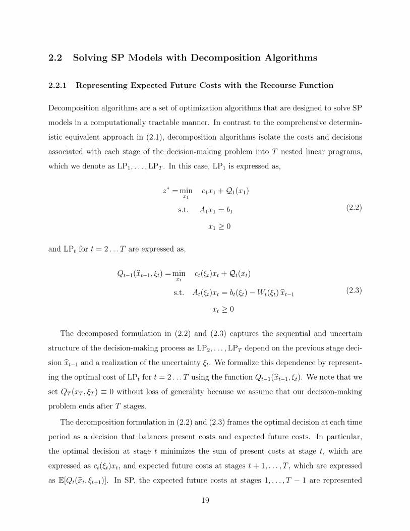
Decomposition algorithms are a set of optimization algorithms that are designed to solve SP

models in a computationally tractable manner. In contrast to the comprehensive determin-

istic equivalent approach in (2.1), decomposition algorithms isolate the costs and decisions

associated with each stage of the decision-making problem into T nested linear programs,

which we denote as LP1, . . . ,LPT . In this case, LP1 is expressed as,

z∗ = minx1

c1x1 +Q1(x1)

s.t. A1x1 = b1

x1 ≥ 0

(2.2)

and LPt for t = 2 . . . T are expressed as,

Qt−1(x t−1, ξt) = minxt

ct(ξt)xt +Qt(xt)

s.t. At(ξt)xt = bt(ξt)−Wt(ξt) x t−1

xt ≥ 0

(2.3)

The decomposed formulation in (2.2) and (2.3) captures the sequential and uncertain

structure of the decision-making process as LP2, . . . ,LPT depend on the previous stage deci-

sion x t−1 and a realization of the uncertainty ξt. We formalize this dependence by represent-

ing the optimal cost of LPt for t = 2 . . . T using the function Qt−1(x t−1, ξt). We note that we

set QT (xT , ξT ) ≡ 0 without loss of generality because we assume that our decision-making

problem ends after T stages.

The decomposition formulation in (2.2) and (2.3) frames the optimal decision at each time

period as a decision that balances present costs and expected future costs. In particular,

the optimal decision at stage t minimizes the sum of present costs at stage t, which are

expressed as ct(ξt)xt, and expected future costs at stages t + 1, . . . , T , which are expressed

as E[Qt(x t, ξt+1)]. In SP, the expected future costs at stages 1, . . . , T − 1 are represented

19

using a function Qt(xt) that omits the expectation operator for clarity. The function Qt(xt)is referred to as the recourse function, and it is defined as

Qt(xt) = E[Qt(xt, ξt+1)] =

∫

Ξt

Qt(xt, ξt+1)ft+1(ξt+1) (2.4)

2.2.2 Approximating the Recourse Function with Cutting Planes

The recourse function Qt(xt) defined in (2.4) represents the expected value of a linear pro-

gram with multiple random parameters. As a result, its value can only be determined

by evaluating a multidimensional integral whose integrand is a linear program. Given the

computational burden involved in evaluating multidimensional integrals, let alone linear

programs, the recourse function should be approximated using few functional evaluations in

order to solve SP models in a computationally tractable way.

Decomposition algorithms achieve this goal by constructing a piecewise linear approxi-

mation to the recourse function Qt(xt) which only requires the evaluation of the multidimen-

sional integral at a limited number of points xt. The resulting approximation is a collection

of supporting hyperplanes to the recourse function at fixed points xt. In the SP literature,

the supporting hyperplanes are referred to as cutting planes or cuts, and the fixed points xt

around which the cuts are built are emphasized using the notation x t. Given a fixed point

x t, a cut is a linear inequality defined as,

Qt(xt) ≥ Qt(x t) +∇Qt(x t)(xt − x t) (2.5)

In practice, the values of the cut parameters Qt(x t, ξt+1) and∇Qt(x t, ξt+1) are determined

using the expected values of the optimal dual variables λt+1 from LPt+1. In particular,

Qt(x t) = E[Qt(x t, ξt+1)] = E[λTt+1(bt(ξt+1)−Wt(ξt+1)]

∇Qt(x t) = E[∇Qt(x t, ξt+1)] = E[λTt+1Wt(ξt+1)]

(2.6)

Given that the linear inequality defined in (2.5) has the same number of variables as LPt, it is

added to the set of existing constraints in LPt in order to improve the current approximation

20

of the recourse function Qt.We note that the benefit of using the optimal dual variables in constructing the cut

parameters is that they can still be determined when LPt+1 is infeasible for a given value of

the previous stage decision x t or the uncertain outcome ξt+1. In such cases, a decomposition

algorithm can use any feasible set of dual variables to construct a cut that will prevent

infeasible instances of LPt+1. This cut is refered to as a feasibility cut, and it is defined as,

Qt(xt) ≥ ∇Qt(x t)(xt − x t) (2.7)

2.2.3 Stopping Procedures

A generic iteration of a decomposition algorithm consists of constructing T−1 cuts to support

the recourse functions Q1, . . . ,QT−1 at a set of fixed values x 1, . . . , xT−1, and adding these

cuts to the linear programs LP1, . . . ,LPT−1. Assuming that the cut parameters in (2.6)

can be calculated exactly, each cut that is added to LPt improves the approximation of the

recourse function Qt, and brings the estimated values of the optimal decision x t and the

optimal cost z t closer to their true values x *t and z *

t. Although it is impossible to determine

the true optimal cost z * of a multistage SP in a general setting, a decomposition algorithm

can produce a lower bound zLB and a upper bound zUB to z *. Given that the value of the

lower bound zLB is monotonically non-decreasing with each iteration and the value of the

upper bound zUB is monotonically non-increasing with each iteration, these bounds can then

be used to stop decomposition algorithms when their difference | zLB − zUB | is smaller than

a user-prescribed tolerance.

The lower bound zLB produced by decomposition algorithms exploits the fact that a

cutting plane approximation of the recourse function consistently underestimates the value

of the true recourse function. This is because the approximation is composed of supporting

hyperplanes to a convex function. In this case, the convexity of the recourse function is

assured as it represents the expected value of a convex function (we note that the cost of a

linear program is a convex function, and the expected value operation preserves convexity).

As a result, we can obtain a lower bound zLB to the true optimal cost z * by considering the

deterministic cost that we incur in the first stage, and the estimated costs that we expect to

21

incur in future stages,

zLB = minx1

c1x1 + Q1(x1) (2.8)

Given that a cutting plane approximation of the recourse function consistently underes-

timates expected future costs, it follows that decisions made with this approximate recourse

function will be suboptimal. By definition, the true expected cost of these suboptimal de-

cisions will exceed the optimal cost of the SP model. In other words, we can obtain an

upper bound to the true optimal cost by calculating the true expected cost of the subop-

timal decisions that are produced with our current approximation of the recourse function.

In the context of a multistage SP, we can calculate the true expected cost of these decisions

by calculating the cost associated with each sequence of uncertain outcomes ξi2, . . . , ξiT , and

forming its expected value. Assuming that there exists K unique sequences of uncertain

outcomes, the upper bound can be calculated as

zUB =K∑

i=1

T∑

t=1

ct(ξit) x t(ξ

it)ft(ξ

it) (2.9)

where,

x it(ξit) = arg min ct(ξ

it)xt + Qt(xit) (2.10)

2.2.4 Overview of Decomposition Algorithms

All decomposition algorithms solve SP models hrough an iterative process that builds cuts

around fixed points x t and adds them to LPt for t = 1, . . . , T − 1. The differences between

these algorithms are primarily based in the way that they choose the fixed points x t around

which they build cuts, the number of cuts that they add with each iteration, and whether

they keep the cuts, drop them after a fixed number of iterations, or refine them with each

iteration. In the context of multistage models, decomposition algorithms can also differ in

the order of the stages at which they build the cuts.

Decomposition algorithms that can be characterized using these traits include the Abridged

Nested Decomposition algorithm from [9], the Cutting Plane and Partial Sampling algorithm

from [6],the ReSa algorithm from [18] and the Stochastic Decomposition algorithm from [17].

22

In this thesis, we restrict our focus on the SDDP algorithm that is presented in [31] due to

its popularity among SP practitioners. The SDDP algorithm uses a greedy procedure to

pick the fixed points x t, adds a single cut to LPt for t = 1, . . . , T − 1 at each iteration, and

permanently keeps the cuts that are produced with each iteration.

We refer the interested reader to [24] for a simple theoretical comparison between decom-

position algorithms, and to [5] for a comprehensive introduction to the theory and practice

of multistage SP.

2.3 Using Monte Carlo Methods in Decomposition Algorithms

The computational bottleneck in solving a multistage stochastic linear program involves

calculating the cut parameters in (2.6), as this requires the evaluation of a multidimensional

integral whose integrand is a linear program. While the cut parameters are easy to calculate

when ξt+1 is a discrete random variable with few outcomes, the calculation is intractable

when ξt+1 is high-dimensional, and impossible when ξt+1 continuous. Subsequently, many SP

practitioners simplify this calculation by modeling the uncertainty in their decision-making

problem using scenario trees.

Scenario trees are discrete in nature, meaning that they either require models that ex-

clusively contain discrete random variables, or a discretization procedure that can represent

continuous random variables using a finite set of outcomes and probabilities. In the latter

case, we note the optimal solution to an SP model in which the continuous random variables

are discretized may differ from the optimal solution of an SP model in which the continuous

random variables are kept in place. Even in situations where a scenario tree approach can

produce accurate solutions, this level of accuracy is difficult to maintain in large-scale prob-

lems with multiple random variables and time periods due to the exponential growth in the

size of the scenario tree. In such cases, scenario trees impose an unnecessary choice between

high-resolution discrete approximations that yield accurate solutions but are difficult to store

and solve, and low-resolution discrete approximations that may yield inaccurate solutions

but are easier to store and solve.

MC methods are an alternative approach to calculate the cut parameters in (2.6). The

23

advantages of this approach are that it can accommodate discrete or continuous random vari-

ables, remain computationally tractable for models with a large number of random variables

and produce estimates of the recourse function whose error does not depend on the number

of random variables in the model. In practice, an MC method involves randomly sampling N

i.i.d. outcomes of the uncertain parameters ξ1t+1 . . . ξ

Nt+1, and estimating the expected values

of the cut parameters in (2.6) through the sample averages,

Qt(x t) ≈ Qt(x t) =1

N

N∑

i=1

Qt(x t, ξit+1)

∇Qt(x t) ≈ ∇Qt(x t) =1

N

N∑

i=1

∇Qt(x t, ξit+1)

(2.11)

Given that the cut parameters in (2.11) are produced by random sampling, it follows that

they are subject to sampling error. In turn, the supporting hyperplane that is produced using

these parameters is also subject to sampling error. We refer to this supporting hyperplane

as a sampled cut, and note that it has the form,

Qt(xt) ≥ Qt(x t) +∇Qt(x t)(xt − x t) (2.12)

2.4 The Impact of Sampling Error in Decomposition Algorithms

In comparison to the exact cut in (2.5), the sampled cut in (2.12) may produce an invalid

approximation of the recourse function. We illustrate this phenomenon in Figures 2-1 and

2-2, where we plot sampled cuts that are produced when a crude MC method is paired with

a decomposition algorithm to solve a simple two-stage Newsvendor model. We note that the

parameters of this model are specified in Section 4.1.1.

Both cuts in this example were constructed using N = 50 samples. For clarity, we plot

a subset of the sample values Q(x , ξi) for i = 1, . . . , N along the vertical line of x , as well as

their sample average 1N

∑Ni=1 Q(x , ξi). In Figure 2-1, we are able to generate a valid sampled

cut, which is valid because it underestimates the true recourse function Q(x) at all values of

x. However, it is possible to generate a sampled cut that in some regions overestimates, and

in other regions underestimates the true recourse function Q(x). We illustrate this situation

24

x

Q(x

)

1

N

N∑

i=1

Q(x, ξi)x

0

-5

-10

-15

-20

-25

-30 0 50 100 150

x∗

x

Q(x, ξi)

Figure 2-1: A valid sampled cut.

x

Q(x

)

x∗

x

1

N

N∑

i=1

Q(x, ξi)

Q(x, ξi)0

-5

-10

-15

-20

-25

-30 0 50 100 150

Figure 2-2: An invalid sampled cut.

25

in Figure 2-2, where the sampled cut excludes the true optimal solution at x∗ ≈ 69 with

z∗ ≈ −20. Assuming that the decomposition algorithm will only generate valid sampled

cuts until it converges, the resulting estimates of x∗ and z∗ will be x ≈ 38 and z ≈ −15,

corresponding to errors of 80% and 25% respectively. We note that the optimal solution x∗

corresponds to the value of x that minimizes the sum of the first-stage costs and the recourse

function, and not the value of x that minimizes the recourse function (although these values

appear to be very close to each other in Figures 2-1 and 2-2).

Even in cases where sampling error in MC estimates of the cut parameters is negligible,

its presence can have a significant impact on the final values of the optimal solution and

optimal cost that are produced from a decomposition algorithm. This is because multiple

quantities that affect the final output in a decomposition algorithm also depend on the cut

parameters, such as the values of the lower bound zLB and the upper bound zUB that are

used to stop the algorithm. In this case, the presence of sampling error means that these

quantities are no longer deterministic values but random distributed estimates and a suitable

statistical procedure is required in order to stop the algorithm. As we demonstrate in Section

5.3, a poorly designed procedure in such situations may stop decomposition algorithm before

it has converged, and thereby result in highly inaccurate estimates of the optimal solution

and the value.

2.5 Reducing Sampling Error through Variance Reduction

It is well-known that the sampling error in MC estimates of the cut parameters can be

expressed as,

SE(Qt(x t)) =

√Var[Qt(x t)] =

σQt(x t)√N

SE(∇Qt(x t)) =

√Var[∇Qt(x t)] =

σ∇Qt(x t)√N

(2.13)

where σQt(x t and σ∇Qt(x t) represent the true standard deviation of the recourse function

and its gradient at the fixed point x t respectively. Although (2.13) implies that we can

reduce the sampling error of MC estimates by increasing the number of samples, the O( 1√N

)

26

convergence rate implies that we have to solve four times as many linear programs in order

to halve the sampling error of the cut parameters. Given the time that is required to solve

a linear program within a large-scale multistage SP model, such an approach is simply not

tractable. As a result, MC methods are typically paired with a variance reduction technique

that can reduce the sampling error of MC estimates by either improving the convergence

rate or reducing the underlying variance of the model.

Variance reduction techniques have generated much interest due to the application of

MC methods across numerous fields; we refer the interested reader to [12], [22] and [25] for

an introductory overview of these techniques.

2.5.1 Stratified Sampling

Stratified sampling techniques are a set of variance reduction techniques that first split the

support Ξ of a random variable ξ into K strata, and generate samples from each of the K

strata. This approach ensures that the samples are randomly distributed while achieving

some variance reduction by spreading samples across the entire sample space. When K = N

strata are used, the stratified sampling technique is referred to as Latin Hypercube Sampling

(LHS), and it produces estimates whose sampling error converges at a rate of O( 1√N

) albeit

within a constant factor of traditional MC methods. We note that this convergence rate

is slow in comparison to state-of-the-art stratified sampling techniques, which can increase

the rate by allocating the N samples in proportion to the variance of each K strata. We

recommend [26] and [40] for a more detailed overview of stratified sampling and LHS.

2.5.2 Quasi-Monte Carlo

Quasi Monte Carlo (QMC) methods are a set of variance reduction techniques that reduce the

sampling error in MC estimates by using a deterministic sequence of points that is uniformly

distributed across multiple dimensions. Examples of such sequences include Halton and

Sobol sequences, whose points are depicted in Figure 2-3.

QMC methods are typically paired with a scrambling algorithm that is specifically de-

signed to randomize a particular sequence of points. Popular examples of scrambling algo-

rithms include the Owen scrambling algorithm for Sobol sequences, and the Reverse-Radix

27

0.0 0.2 0.4 0.6 0.8 1.00.0

0.2

0.4

0.6

0.8

1.0

U15

U30

0.0 0.2 0.4 0.6 0.8 1.00.0

0.2

0.4

0.6

0.8

1.0

U15

Figure 2-3: Cross section of points from a Halton sequence (green) and a Sobol sequence(blue).

2 algorithm for Halton sequences. As shown in Figure 2-4, scrambling randomizes the points

from QMC sequences while maintaining their uniformity across each dimension.

0.0 0.2 0.4 0.6 0.8 1.00.0

0.2

0.4

0.6

0.8

1.0

U15

U30

0.0 0.2 0.4 0.6 0.8 1.00.0

0.2

0.4

0.6

0.8

1.0

U15

Figure 2-4: Cross section of points from a randomized Halton sequence (green) and a ran-domized Sobol sequence (blue).

In the cases that an MC estimate is produced using N randomized points from a QMC

method, it has been shown that the sampling error in the estimates converges at an improved

rate of O( logNN1.5

0.5(D−1)) so long as the recourse function is smooth. For a more detailed

introduction to QMC methods, we refer the reader to [28] and [29].

2.5.3 Importance Sampling

Importance sampling is a variance reduction technique that aims to reduces the sampling

error in MC estimates by generating samples from an importance sampling distribution g,

as opposed to the original sampling distribution f . When samples are generated from an

28

importance sampling distribution g, the recourse function can be calculated as,

Q(x ) = Ef [Q(x , ξ)]

=

∫

Ξ

Q(x , ξ)f(ξ)dξ

=

∫

Ξ

Q(x , ξ)f(ξ)g(ξ)

g(ξ)dξ

=

∫

Ξ

Q(x , ξ)f(ξ)

g(ξ)g(ξ)dξ

=

∫

Ξ

Q(x , ξ)Λ(ξ)g(ξ)dξ

= Eg[Q(x ,Λ(ξ)]

(2.14)

In (2.14), the function Λ : Ξ→ R,

Λ(ξ) =f(ξ)

g(ξ)(2.15)

is typically refered to as the likelihood function, and it is used to correct the bias that is

produced by the fact that we generated samples from the importance sampling distribution

g instead of the original distribution f . Once we select a suitable important sampling distri-

bution g, we can generate a set of N i.i.d. samples ξ1, . . . , ξN , and construct an importance

sampling estimate of the recourse function as,

Q(x ) =1

N

N∑

i=1

Q(x , ξi)Λ(ξi) (2.16)

In theory, importance sampling simply reflects a change in the measure with which we

compute the recourse function at a fixed point x . Accordingly, any distribution g can be used

as an importance sampling distribution as long as the likelihood function Λ is well-defined

over the support of f . In other words, the importance sampling distribution g should be

chosen so that g(ξ) > 0 at all values of ξ where f(ξ) > 0. When this requirement is satisfied,

the sampling error of importance sampling methods also converges at a rate of O( 1√N

), albeit

with a different constant factor than traditional MC methods.

Ideally, an importance sampling distribution g is one that can generate samples at regions

where Q(x )f(ξ) attains high values, which are referred to as the important regions of the

29

recourse function. Nevertheless, we stress that the importance sampling distribution g should

also be able to evaluate the probability g(ξ) of each sample to a high degree of accuracy.

This is because misspecified values of the importance sampling distribution g(ξ) will produce

misspecified values of the likelihood Λ(ξ), and produce an importance sampling estimate that

is highly biased.

We refer the interested reader to [2] for a more detailed review of importance sampling.

2.5.4 IDG Importance Sampling

Importance sampling was first applied to SP in [7] and [20]. We refer to this importance

sampling distribution proposed as the Infanger-Dantzig-Glynn (IDG) distribution. The IDG

distribution has been shown to mitigate the issues associated with the use of sampled cuts in

decomposition algorithms that we cover in Section 2.3. Unfortunately, the IDG distribution

in these papers makes several assumptions which severely limit its applicability to a broad

range of SP models.

To begin with, the IDG distribution can only be used in SP models where the uncertainty

is modeled using discrete random variables. As a result, any SP model where we can use the

IDG distribution for importance sampling is subject to the same computational issues that

we attribute to the scenario tree approach in Section 2.3.

Moreover, the IDG distribution assumes that the cost surface Q(x , ξ) is additively sepa-

rable in the random dimensions, meaning that

Q(x , ξ) ≈D∑

d=1

Qd(x , ξd) (2.17)

In SP models where such an approximation does not hold, the sampling error in the IDG

estimate will still converges at a rate that is O( 1√N

) but with a much larger constant than

traditional MC methods. In such cases, the IDG distribution produces estimates that are

have high rates of error.

A final issue with the IDG distribution is that it requires practioners to know or determine

the value of random outcome ξ which minimizes the cost surface Q(x , ξ). In a general setting,

the only way to determine the value is to perform an exhaustive search across all the uncertain

30

outcomes ξ ∈ Ξ.

It is true that there exist practical ways to work around these assumptions. However,

we note that our numerical experiments in Section 4.8.1 suggest that the performance of

the IDG distribution is critically determined by these factors. In turn, there remains a need

for an alternative approach importance sampling that does not suffer from such issues for a

broader range of SP models.

31

THIS PAGE INTENTIONALLY LEFT BLANK

32

Chapter 3

The Markov Chain Monte Carlo

Approach to Importance Sampling

In this chapter, we introduce the zero-variance importance sampling distribution (Section

3.1.1) and provide an overview of MCMC algorithms (Section 3.1.2) and KDE algorithms

(Section 3.1.3). We then proceed to explain how these algorithms can be combined to

build an importance sampling distribution that approximates the zero-variance distribution

(Section 3.2) - a procedure that we refer to as the Markov Chain Monte Carlo Approach

to Importance Sampling (MCMC-IS). Having introduced MCMC-IS, we present a simple

MCMC-IS implementation to illustrate how MCMC-IS can be used in practice (Section 3.3).

We end this chapter with a discussion of the theoretical aspects of MCMC-IS where we cover

the ingredients of a convergence analysis (Section 3.4).

33

3.1 Foundations of the Markov Chain Monte Carlo Approach to

Importance Sampling

3.1.1 The Zero-Variance Distribution

Importance sampling is most effective in the context of SP models when the importance

sampling distribution g can generate samples from regions that contribute the most to the

value of the recourse function Q(x ). In fact, when an importance sampling distribution can

generate samples according to the exact importance of each region as,

g∗(ξ) =|Q(x , ξ)|f(ξ)

Ef [|Q(x , ξ)|](3.1)

then the variance and sampling error of its estimates will be minimized (see [2]). Moreover,

if the recourse function Q(x, ξ) > 0 for all ξ ∈ Ξ, then the importance sampling distribution

g* can produce a perfect estimate of the recourse function with only a single sample ξ1 as,

Q(x ) =1

N

N∑

i=1

Q(x , ξi)Λ(ξi)

= Q(x , ξ1)f(ξ1)

g*(ξ1)

= Q(x , ξ1)f(ξ1)

Q(x , ξ1)f(ξ1)

Ef [Q(x , ξ)]

= Ef [Q(x , ξ)]

(3.2)

In light of this fact, the importance sampling distribution g* is often referred to as the

zero-variance importance sampling distribution. The problem with using the zero-variance

distribution g* in practice is that it requires knowledge of Ef [|Q(x, ξ)|], which is the quantity

that we sought to compute in the first place. In turn, we are faced with a ”curse of circularity”

in that we can use the zero-variance distribution g* to construct perfect estimates if and only

if we already have a perfect estimate of Ef [|Q(x , ξ)|].

34

3.1.2 Overview of MCMC Algorithms

MCMC algorithms are an established set of MC methods that can sample from a distribution

which is known up to a normalizing constant. In contrast to other MC methods, MCMC

algorithms generate a serially correlated sequence of samples ξ1, . . . , ξM . This sequence

constitutes a Markov chain whose stationary distribution is equal to the distribution that

we wish to sample from.

The simplest MCMC algorithm is the Metropolis-Hastings algorithm from [27], which we

refer to throughout this thesis and cover in detail in Section 3.3. The Metropolis-Hastings

algorithm generates samples from a target distribution g by proposing new samples through

a proposal distribution q and accepting each sample as the next state of the Markov chain

using a simple accept-reject rule.

In addition, we refer to the Adaptive Metropolis algorithm from [14] in Section 4.5, which

uses a random walk distribution as the proposal distribution in the Metropolis-Hastings

algorithm and automatically scales the step-size within this distribution. Lastly, we cover

the Hit-and-Run algorithm from [39] in Section 4.6, which is designed to generate samples

within bounded regions by using an accept-reject approach that resembles the Metropolis-

Hastings algorithm.

We note that numerous other MCMC algorithms have been developed for different prac-

tical applications, and many of them can be used in the importance sampling framework

that we present in this thesis. We refer the interested reader to [1],[11], and [13] for a

comprehensive overview of the theoretical and practical aspects of MCMC algorithms.

35

3.1.3 Overview of KDE Algorithms

KDE algorithms are an established set of techniques that are designed to reconstruct a

continuous probability distribution from a finite set of samples. Given a set of a M samples,

ξ1, . . . , ξM , the output of a KDE algorithm is an empirical probability distribution function,

gM(ξ) =1

M

M∑

i=1

KH(ξ, ξi) (3.3)

where the function KH is referred to as a kernel function, and the matrix H ∈ RD×D

is referred to as the bandwidth matrix. We note that the kernel function KH in (3.3)

determines the probability of the region that surrounds each of the M samples ξ1, . . . ξM

while the bandwidth matrix H determines the width of the region spanned by the kernel

function KH at each sample.

In theory, the kernel function KH has to be chosen so that the output from the KDE

algorithm gM(ξ) is a probability distribution. In the multidimensional case, this requires a

function KH such that

KH(·, ·) ≥ 0∫

Ξ

KH(ξ, ·)dξ = 1∫

Ξ

ξKH(ξ, ·)dξ = 0∫

Ξ

ξξTKH(ξ, ·)dξ = 0

(3.4)

Assuming that these conditions are satisfied, the kernel function is said to be well-behaved,

and its shape does not significantly impact the empirical distribution gM that is produced

by a KDE algorithm. In practice, KH is typically set as the product of D one-dimensional

kernel functions K1, . . . , KD that are symmetric around the origin in order to reduce the

computational burden associated with KDE algorithms. Examples of such functions include

the Gaussian, Laplacian or Epatchenikov kernel functions, which we plot in Figure 3-1.

In comparison to the impact of the kernel function KH , the bandwidth matrix H can

substantially impact the accuracy of an empirical distribution produced by gM . Although the

36

−2 0 20.0

0.2

0.4

0.6

0.8

1.0

ξ

K(ξ

)

−2 0 20.0

0.2

0.4

0.6

0.8

1.0

ξ

−2 0 20.0

0.2

0.4

0.6

0.8

1.0

ξ

Figure 3-1: Laplacian (green), Gaussian (red) and Epanetchnikov (blue) kernels functions.

bandwidth matrix H is only required to be symmetric and positive definite, KDE algorithms

automate the choice of H through a bandwidth estimator, which determines the value of

each entry within H in order to minimize the error in gM according to different metrics and

assumptions. We include an overview of bandwidth estimators in Table 3.1

We note that there exists many different KDE algorithms that can be applied in the

importance sampling framework that we present in this thesis. We refer the interested

reader to [8], [35] and [38] for an more detailed overview of these algorithms.

3.2 The Markov Chain Monte Carlo Approach to Importance

Sampling

The importance sampling framework that we present in this thesis is motivated by two

insights regarding the zero-variance distribution as defined in (3.1).

The first insight is that the zero-variance distribution is known up to a normalizing

constant E[|Q(x , ξ)|]. This implies that we can generate samples from this distribution using

an MCMC algorithm. Unfortunately, we cannot use these samples to form a perfect estimate

even as they belong to the zero-variance distribution. This is because we still need to evaluate

the likelihood of each sample as defined in (2.15). In this case, the likelihood of a sample ξ

is given by,

Λ∗(ξ) =Ef [|Q(x , ξ)|]|Q(x , ξ)| (3.5)

which is impossible to compute because it depends on Ef [|Q(x , ξ)|]. Our inability to use the

37

Approach Optimal Bandwidth h∗ Parameters

Mean IntegratedSquared Error

argminh

E[ ∫

(gM (ξ)− g(ξ))2dξ]

-

AsymptoticMean IntegratedSquared Error

M−15

(R(K)

R(g*′′

)σ4K

) 15 R(K) =

∫K2(ξ)dξ,

σ2K =

∫ξ2K(ξ)dξ

GaussianRule of Thumb

(4σ5

3n

) 15

σ = min(S, IQR

1.34

)

S and IQR denote the samplestandard deviation and

interquartile range of the samples

Leave-One-OutCross Validation

argminh

∫g2M (ξ)dξ − 2

M

M∑i=1

gM,−i(ξi)gM,−i denotes the distribution gM

that is formed using all samplesexcept ξi

Table 3.1: Bandwidth estimators for KDE algorithms.

38

samples that we generate from the zero-variance distribution to form a perfect estimate leads

us to the second insight: while we cannot use the samples to form an importance sampling

estimate, we can use them to reconstruct an approximation of the zero-variance distribution

by using a KDE algorithm.

In particular, assuming that we have generated M samples from the zero-variance distri-

bution using an MCMC algorithm, we can use a KDE algorithm to reconstruct an approxi-

mate zero-variance distribution gM from these samples. With the approximate zero-variance

distribution gM , we can then produce an importance sampling estimate of the recourse func-

tion by generating N additional samples ξ1, . . . , ξN from gM . As we can now specify both

the original distribution f and the distribution that we used to generate these samples gM ,

we can evaluate the likelihood of each sample as,

Λ(ξ) =f(ξ)

gM(ξ)(3.6)

and form the importance sampling estimate as,

Q(x ) =1

N

N∑

i=1

Q(x , ξi)Λ(ξi) (3.7)

The samples ξ1, . . . , ξN will not originate from the true zero-variance distribution g∗.

Nevertheless, they can still be used to produce an effective importance sampling estimate

provided that the KDE algorithm is able to construct a gM that is similar to g∗. Given that

the importance sampling distribution gM will only be an approximation of the zero-variance

distribution g*, it follows that the estimates that are produced through this framework

will typically not have zero variance and zero sampling error. Nevertheless, the process of

generating samples in regions that contribute most to the value of the recourse function will

still lead to importance sampling estimates with low-variance and low-sampling error.

We note that it is possible to generate samples using an MCMC algorithm and then

directly construct an importance sampling estimate of the recourse function by using a

self-normalized importance sampling scheme, or by using a KDE algorithm to estimate the

probability g∗(ξi) for i = 1, . . . ,M . We note, however, that resampling from the approxi-

39

mate zero-variance distribution gM ultimately produces more accurate importance sampling

estimates. This is due to the fact that importance sampling estimates are highly sensitive

to the likelihood of each sample, and the resampling process allows us exactly determine

the likelihood of each sample used to construct the importance sampling estimate. In con-

trast, the use of an MCMC-only approach will approximate the likelihood of each sample

and ultimately produce a biased importance sampling estimate. Generating samples from

gM is also beneficial in that the samples are independent and the kernel functions are easy

to sample from, especially when compared to the computational overhead involved in the

MCMC sampling process. In practice, we therefore construct gM using modest values of M

and then construct an importance sampling estimate Q(x ) using large values of N .

3.3 MCMC-IS in Practice

In this section, we present a simple implementation of MCMC-IS that can be used to generate

importance sampling estimates with low sampling error. Our simple implementation uses

a Random Walk Metropolis-Hastings algorithm to generate samples from the zero-variance

distribution, and a Gaussian product kernel and leave-one-out cross validation bandwidth

estimator to construct the approximate zero-variance distribution. We include a step-by-step

explanation of how to generate an importance sampling estimate using this implementation

in Algorithm 1.

The Metropolis-Hastings algorithm uses a simple accept-reject procedure in order to

generate a Markov chain that has (3.1) as its stationary distribution. In the k-th step,

the algorithm generates a proposed sample ζk using a proposal distribution q(· | ξk), which

typically depends on the current sample ξk. Together, the proposed sample, the current

sample and the target distribution are used to evaluate an acceptance probability, a(ξk, ζk).

The proposed sample is accepted with probability a(ξk, ζk), in which case the Markov Chain

transitions to the proposed sample ξk+1 := ζk. Otherwise, the proposed sample is rejected

with probability 1− a(ξk, ζk), in which case the Markov chain remains at its current sample

ξk+1 := ξk.

In our simple implementation, we choose to a random walk process to propose the samples

40

in the Metropolis-Hastings algorithm. This implies that the proposed sample ζk is generated

as,

ζk = ξk + vk (3.8)

where vk is a Gaussian random variable with mean 0 and covariance matrix Σ. When new

samples are proposed through a random walk process, the proposal distribution is symmetric

and the acceptance probability can be expressed as,

a(ξk, ζk) = min

|Q(x , ζk)|f(ζk)

|Q(x , ξk)|f(ξk), 1

(3.9)

In terms of KDE algorithm, we use a Gaussian product kernel function,

KH(ξ, ξi) =D∏

k=1

1√2πhk

exp

((ξk − ξi,k)2

2h2k

)(3.10)

where the bandwidth matrix H is a D × D diagonal matrix that contains the bandwidth

parameters of each dimension h1, . . . , hD along its diagonal. In this case, we use a one-

dimensional leave-one-out cross validation estimator to estimate the value of the bandwidth

parameter hk separately for each dimension k. The exact parameters for this bandwidth

estimator are defined in Table 3.1.

We note that we use this simple MCMC-IS implementation to generate the majority of

the numerical results in Chapters 4 and 5 because it is straightforward to implement and

does not depend on a restrictive set of assumptions. The quality of numerical results that

we achieve with this admittedly simple implementation in these chapters only reinforces the

potential of MCMC-IS, as more efficient implementations of MCMC-IS would only further

increase the advantages of our framework. It is true that this simple implementation can

also lead to certain challenges in practice; we refer to these challenges throughout Chapter 4

and provide recommendations to fix them by using different MCMC and KDE algorithms.

41

Algorithm 1 Markov Chain Monte Carlo Importance Sampling (MCMC-IS)

Require: x : previous stage decisionRequire: M : number of samples to generate using the MCMC algorithmRequire: N : number of samples to generate using the approximate zero-variance distribu-

tionRequire: ξ0: starting sample for the MCMC algorithmRequire: q(· | ξk): proposal distribution for the MCMC algorithmRequire: KH : kernel function for the KDE algorithmRequire: H: bandwidth matrix for the KDE algorithm

Step 1: Generate Samples from the Zero-Variance Distribution using MCMC

1: Set k = 02: Given the current sample ξk, generate ζk ∼ q(· | ξk).3: Generate a uniform random variable u ∼ U ∈ (0, 1).4: Transition to the next sample according to,

ξk+1 =

ζk if u ≤ a(ξk, ζk)

ξk otherwise

where,

a(ξk, ζk) = min

|Q(x , ζk)|f(ζk)q(ξk|ζk)|Q(x , ξk)|f(ξk)q(ζk|ξk)

, 1

5: Let k ← k + 1. If k = M then proceed to Step 6. Otherwise return to Step 2.

Step 2: Reconstruct an Approximate Zero-Variance Distribution using KDE

6: For each sample generate from MCMC, reconstruct the approximate zero-variance dis-tribution as,

gM(ξ) =1

M

M∑

i=1

KH(ξ, ξi)

Step 3: Resample from the Approximate Zero-Variance Distribution to

Form an Importance Sampling Estimate

7: Generate N new samples from gM and form the importance sampling estimate,

Q(x ) =1

N

N∑

i=1

Q(x , ξi)f(ξi)

gM(ξi)

42

3.4 MCMC-IS in Theory

The convergence properties of MCMC-IS depend on two sources of error: the first is due

to the MCMC algorithm used to generate samples from the zero variance distribution; the

second is due to the KDE algorithm used to construct the approximate zero-variance distri-

bution.

The main convergence condition in terms of the MCMC algorithm requires that the sam-

ples generated by the MCMC algorithm form a Markov chain whose stationary distribution

is the zero-variance distribution. This requires the underlying Markov chain in the MCMC

process to be irreducible and aperiodic. The irreducibility property means that the chain

can eventually reach any subset of the space from any state. The aperiodicity property

means that the chain cannot return to a subset of the space in a predictable manner. Formal

definitions of these properties can be found in [33]. The first step in the convergence analysis

is to show that these two conditions are satisfied.

In order to control the error due to the KDE algorithm, we need to ensure that the

number of samples are generated by the MCMC algorithm, M , is large enough, and that the

bandwidth, hk, is small enough. In particular, if (MhD)−1 → ∞, h → 0 as M → ∞, and

the distribution is approximated as,

gM(ξ) =1

M

M∑

i=1

KH(ξ, ξi) = (MhD)−1 1

M

M∑

i=1

K

(ξ − ξih

)(3.11)

then it has been shown that gM will probabilistically converge to g* under the total variation

norm in [8]. Applying this result to MCMC-IS is not straightforward. The complexity stems

from the fact that previous convergence proofs for the KDE algorithm assume that samples

are generated from g*, whereas in our framework these samples are generated from a Markov

chain whose stationary distribution is g*.

A final issue that may affect the convergence of MCMC-IS is the fact that the sam-

ples generated through the MCMC algorithm are typically correlated, while the samples

used in many treatments of KDE algorithms assume that the samples used to construct a

KDE distribution are independent. Our numerical experiments from Chapter 4 suggest that

43

MCMC-IS can converge even when there is a degree of correlation between MCMC samples.

However, we note that there is some theoretical evidence that KDE algorithms do not nec-

essarily require the samples independence between the samples. In particular, theoretical

results in [15] suggest that KDE algorithms can construct accurate empirical distributions

using correlated samples so long as they use a different bandwidth estimator. In cases where

this bandwidth estimator is not available, we note that authors of [15] also state that a

leave-one-out bandwidth estimator may provide an adequate approximation.

44

Chapter 4

Numerical Experiments on Sampling

Properties

In this chapter, we illustrate the sampling properties of MCMC-IS using numerical experi-

ments based on a Newsvendor model. We begin by introducing a simple Newsvendor model

with two random variables and two stages (Section 4.1), and explain how it can be extended

to include multiple random variables (Section 4.1.2) and multiple time periods (Section

4.1.3). We then use this model to illustrate how the importance sampling distribution pro-

duced by MCMC-IS can sample from important regions of the recourse function (Section

4.3). Next, we demonstrate how the number of MCMC samples used in MCMC-IS can affect

the error in MCMC-IS estimates (Section 4.4), and provide insight as to how this relation-

ship scales according to the number of random dimensions in the recourse function (Section

4.4.1). In subsequent numerical experiments, we highlight how the acceptance rate of an

MCMC algorithm is related to the accuracy and computational efficiency of MCMC-IS esti-

mates (Section 4.5), show how to modify MCMC-IS in order to generate samples in bounded

regions (Section 4.6), and examine how the choice of kernel functions and bandwidth es-

timators in the KDE algorithm of MCMC-IS can impact the estimates that are produced

(Section 4.7). We end this chapter with a comparison between MCMC-IS and other variance

reduction methods that can be applied to SP models (Section 4.8).

45

4.1 The Newsvendor Model

4.1.1 A Simple Two-Stage Model

The test problem in our numerical experiments in Chapters 4 and 5 is a two-stage Newsvendor

model with uncertain demand and sales prices. The first-stage decision-making problem in

our model is a linear program defined as,

z∗ = minx

x+Q(x)

s.t. x ≥ 0

(4.1)

and the recourse function is the expected value of the linear program defined as,

Q(x , ξ) = miny1,y2

− p(ξ2)y1 − ry2

y1 ≤ d(ξ1)

y1 + y2 ≤ x

y1, y2 ≥ 0

(4.2)

In (4.2), x is a scalar that represents the quantity of newspapers purchased in the first stage,

r = 0.10 is a scalar that represents the price of recycling unsold newspapers, and ξ = (ξ1, ξ2)

is a two-dimensional random vector that represents the uncertainty in demand d(ξ1) and

sales price p(ξ2) of newspapers.

In our numerical experiments, we investigate the sampling properties of MCMC-IS by

pairing this model with three separate distributions: a lower-variance lognormal distribution,

a higher-variance lognormal distribution, and a multimodal rare-event distribution. The

parameters used to generate the demand and sales price for these distributions are specified

in Table 4.1.

4.1.2 A Multidimensional Extension

The D-dimensional Newsvendor model is a multidimensional extension of the Newsven-

dor model specified in Section 4.1.1. In this extension, we consider a problem where the

46

DistributionLower-Variance

LognormalHigher-Variance

LognormalMultimodalRare-Event

(ξ1, ξ2) N(0, 12 × I2) N(0, 22 × I2) N(0, 12 × I2)

d(ξ1) 100 exp(ξ1) 100 exp(ξ1)100 exp

( ξ212 −

(ξ1+3)2

8

)

+100 exp

( ξ212 −

(ξ1+1)2

8

)

p(ξ2) 1.50 exp(ξ2) 1.50 exp(ξ2)1.50 exp

( ξ222 −

(ξ2+3)2

8

)

+1.50 exp

( ξ222 −

(ξ2+1)2

8

)

Table 4.1: Parameters of demand and sales price distributions for the Newsvendor model.

Newsvendor has to sell D2

different types of newspapers which have the same demand and

sales price distribution. The recourse function of the D-dimensional Newsvendor model can

be expressed as,

QD(x ) =

D2∑

i=1

Qi(x i) (4.3)

where Qi(x i) denotes the 2-dimensional recourse function used to represent the expected

future costs associated with a single type of newspaper as in (4.2).

4.1.3 A Multistage Extension

The T -stage Newsvendor model is a multistage extension of the Newsvendor model specified

in Section 4.1.1. In this extension, we consider a problem where the Newsvendor buys and

sells a single type of newspapers over T consecutive days. We assume that any newspapers

that are to be sold on day t+ 1 have to be bought on day t, and that any unsold newspapers

at the end of day t + 1 have to be recycled at a price of r. These assumptions allow us

to extrapolate the true values of optimal solution x * and optimal cost z * for a T -stage

Newsvendor model from their corresponding values for the Newsvendor model specified in

Section 4.1.1. In particular, we reason that the optimal cost z * scales additively with the

47

number of time periods, and the optimal solution x * remains the same.

4.2 Experimental Setup

4.2.1 Experimental Statistics

The advantages of using the two-stage, two-dimensional Newsvendor model in Section 4.1.1

are that the relevant distributions can be easily visualized, and that we can determine the

true value of the recourse function at different values of x using state-of-the-art numerical

integration procedures. In turn, we can also determine the true values of the recourse

function for the multidimensional and multistage extensions of the Newsvendor problem

that are specified in Sections 4.1.2 and 4.1.3.

By knowing the true values of the recourse function for these SP models, we can con-

sider both the error and the variance of the estimates that are produced in our numerical

experiments. Table 4.2 provides an overview of the different statistics that we report in

Sections 4.3 - 4.8. We note that the statistics in these sections have been generated using

R = 100 repetitions, and have been normalized for clarity. We note that that all the results

for the MCMC-IS method have been generated using Mγ

+ N functional evaluations as we

explain further in Section 4.5, where γ denotes the acceptance rate of the MCMC algorithm

in MCMC-IS.

4.2.2 Implementation

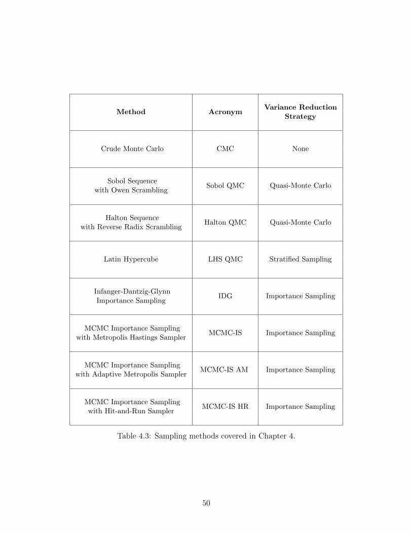
Table 4.3 summarizes the different sampling methods that refer to in Sections 4.3 - 4.5.

Unless otherwise stated, we produced all results for these methods in MATLAB 2012a. In

particular, we used a built-in Mersenne-Twister algorithm to generate the uniform random

numbers for the CMC, LHS, IDG and MCMC-IS sampling methods. Similarly, we used

built-in Owen and Reverse-Radix scrambling algorithm to randomize the sequences that

we generated for Sobol QMC and Halton QMC methods. Most of the results for MCMC-

IS were generated using the simple implementation described in Section 3.3. We built all

approximate importance sampling distributions for MCMC-IS using the MATLAB KDE

Toolbox, which is available online at http://www.ics.uci.edu/~ihler/code/kde.html.

48

Statistic Formula Description

MSE(Q)

√√√√ 1

R

R∑

i=1

(Q(x )− Q(x )i)2mean-squared error of R

estimates of the value of therecourse function Q at x

SE(Q) 1

R

R∑

i=1

1

N

1

N − 1

√√√√(Q(x )i −

1

N

N∑

j=1

Q(x , ξj)

)2mean of R estimates of

standard error in the value ofthe recourse function Q at x

MSE(g)1

R

R∑

i=1

1

N

√(g(ξi)− g(ξi))2

mean-squared error of Rapproximations of the

zero-variance distributions atx ; the ξis are specified by a

100× 100 grid on Ξ

Table 4.2: Sampling statistics reported in Chapter 4.

4.3 Sampling from the Important Regions

Importance sampling is most effective when an importance sampling distribution can gener-

ate samples from regions that contribute the most to the value of the the recourse function.

Such regions are referred to as the important regions of the recourse function, and occur at

points where |Q(x , ξ)|f(ξ) attains large values. Accordingly, the major difference between

MCMC-IS and other MC methods is that MCMC-IS generates samples at important areas

of the recourse function using the importance sampling distribution gM .

We illustrate this difference by plotting the location of the samples that are used to esti-

mate the recourse functionQ(x ) at x = 50 for a Newsvendor model assuming a lower-variance

lognormal distribution in Figure 4-1, and Newsvendor model paired with a a multimodal

rare-event distribution in Figure 4-2.

As shown in Figures 4-1 and 4-2, the samples that are generated using the MCMC-

IS importance sampling distribution gM are located at important regions of the recourse

function, where |Q(x , ξ)|f(ξ) attains high values. In contrast, the samples generated using

49

Method AcronymVariance Reduction

Strategy

Crude Monte Carlo CMC None

Sobol Sequencewith Owen Scrambling

Sobol QMC Quasi-Monte Carlo

Halton Sequencewith Reverse Radix Scrambling

Halton QMC Quasi-Monte Carlo

Latin Hypercube LHS QMC Stratified Sampling

Infanger-Dantzig-GlynnImportance Sampling

IDG Importance Sampling

MCMC Importance Samplingwith Metropolis Hastings Sampler

MCMC-IS Importance Sampling

MCMC Importance Samplingwith Adaptive Metropolis Sampler

MCMC-IS AM Importance Sampling

MCMC Importance Samplingwith Hit-and-Run Sampler

MCMC-IS HR Importance Sampling

Table 4.3: Sampling methods covered in Chapter 4.

50

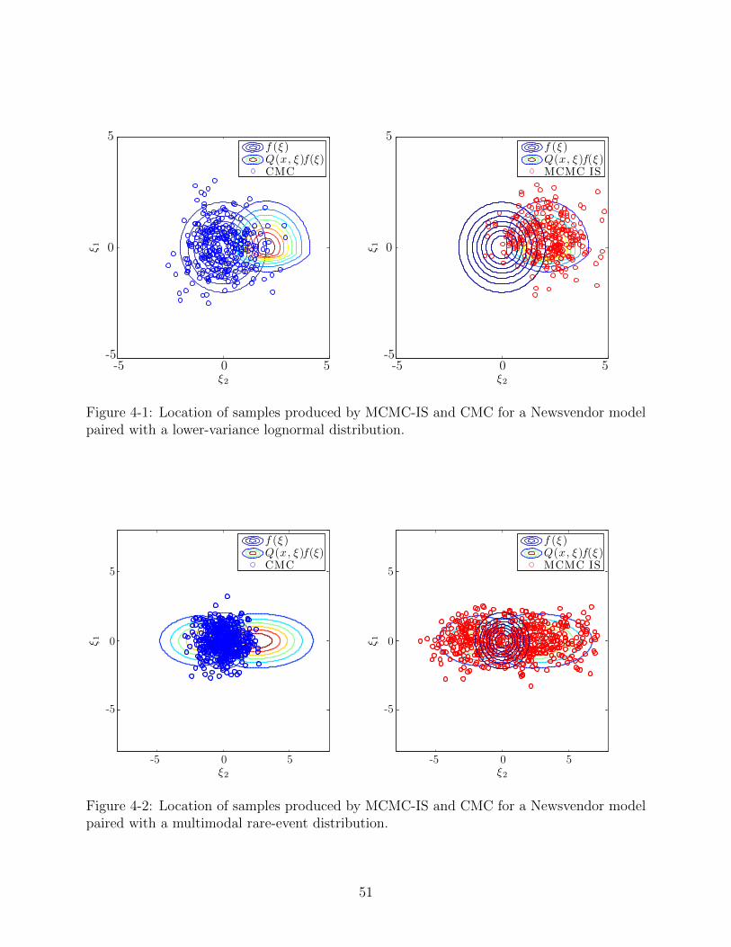
ξ2

ξ1

f (ξ)Q(x, ξ)f(ξ)CMC

ξ2ξ1

f (ξ)Q(x, ξ)f(ξ)MCMC IS

0

0

0

5

5 -5 -5

0

0

5

5 -5 -5

Figure 4-1: Location of samples produced by MCMC-IS and CMC for a Newsvendor modelpaired with a lower-variance lognormal distribution.

ξ2

ξ 1

ξ2

ξ 1

0

0

5

5

-5

-5 0 5 -5

0

5

-5

f (ξ)Q(x, ξ)f(ξ)CMC

f (ξ)Q(x, ξ)f(ξ)MCMC IS

Figure 4-2: Location of samples produced by MCMC-IS and CMC for a Newsvendor modelpaired with a multimodal rare-event distribution.

51

CMC are located in regions where the original distribution f(ξ) attains high values. The

contours in these figures demonstrate how f(ξ) and |Q(x , ξ)|f(ξ) may not only have different

shapes but may also be centered around different points.

The fact that MCMC-IS can generate samples in these regions for both distributions

demonstrates the adaptive nature of our framework. This property is especially important

in the context of decomposition algorithms because the important areas of the recourse

function Q(x ) can vary substantially according to the previous-stage decision x .

4.4 The Required Number of MCMC Samples

In Figures 4-3(a) and 4-3(b), we show how the error in the approximate zero-variance dis-

tribution gM and the error in the recourse function estimate Q changes according to the

number of MCMC samples, M , used in MCMC-IS. In this case, we consider estimates of

the recourse function Q(x ) at x = 50 for a Newsvendor model assuming a lower-variance

lognormal distribution, and we construct each estimate using N = 16000 samples generated

from the approximate zero-variance distribution gM .

As shown, increasing M reduces the error in the approximate importance sampling dis-

tribution gM and subsequently also reduces the error in resulting importance sampling esti-

mates of the recourse function Q. Although the convergence in the density error in gM and

the sampling error in Q appears to be steady, we note that increasing the number of MCMC

samples is often hard to justify, as these graphs show that we can obtain estimates with

error rates of less than 1% using only M = 1000 samples in the MCMC step and N = 16000

samples in the resampling step. This is a positive result as the MCMC algorithm represents

the most computationally expensive part of our framework.

A possible explanation for this empirical observation is that if the approximate zero-

variance distribution gM qualitatively agrees with the true zero-variance distribution g*, then

the estimates produced using gM should have properties that are similar to the estimates

produced using g*. In Figure 4-4(a), we provide evidence that gM qualitatively agrees with

g* by plotting its contours for different values of M .

52

1 2 3 4 5 6 7 8

2.00

2.50

3.00

×10−3

M × 103

MS

E(g

)

(a)

1 2 3 4 5 6 7 8

2.00

4.00

6.00

8.00

×10−3

M × 103

MS

E(Q

)

(b)

Figure 4-3: Convergence of gM (a) and Q(x ) (b).

4.4.1 The Curse of Dimensionality

In this section, we examine how the required number of MCMC samples M changes as we

increase the number of random variables D in the recourse function Q(x ). In particular,

we consider the recourse function Q of a D-dimensional Newsvendor model from Section

4.1.2, where the Newsvendor sells D2

different types of newspapers. We use a lower-variance

lognormal distribution to specify the demand and sales price for each type of newspaper,

and estimate the recourse function at x = 50e where e is a D2× 1 vector of ones.

As we describe in Section 4.1.2, the recourse function of the D-dimensional Newsvendor

model can be expressed as the sum of D2

recourse functions of our 2-dimensional Newsvendor

model (note that we only consider even multiples of D in our experiment). This implies

that the true standard deviation of the recourse function in our D-dimensional model is√

D2

larger than the true standard deviation of the recourse function in our 2-dimensional model.

We account for this difference in our experiment by scaling the number of samples N used

construct the recourse function estimate by√

D2

. In addition, we also account for the fact

that we will require more samples to construct an approximate zero-variance distribution for

a D-dimensional recourse function by scaling the number of MCMC samples M in proportion

to D.

Our results in Figure 4.4.1 demonstrate how the error in our estimates increases with the

53

ξ1

ξ 2

4

3

2

1

0

-1

-2

-3 -3 -2 -1 0 1 2 3

(a) g∗ξ1

ξ 2

4

3

2

1

0

-1

-2

-3 -3

-2 -1 0 1 2 3

(b) g500

ξ1

ξ 2

4

3

2

1

0

-1

-2

-3 -3 -2 -1 0 1 2 3

(c) g1000

ξ1

ξ 2

4

3

2

1

0

-1

-2

-3 -3 -2 -1 0 1 2 3

(d) g10000

Figure 4-4: Contours of g* (a) and gM for different values of M (b)-(d).

54

0.5 1.0 1.5 2.0 2.5 3.0 3.5 4.00.00

0.02

0.04

0.06

0.08

0.10

MD−1 × 103

MS

E(Q

)

(a)

0.5 1.0 1.5 2.0 2.5 3.0 3.5 4.00.00

0.02

0.04

0.06

0.08

0.10

MD−1 × 103

MS

E(Q

)

D = 2

D = 4

D = 6

D = 8

(b)

Figure 4-5: Convergence of Q(x ) using N = 16000×√

D2

samples (a), and N = 64000×√

D2

samples (b).

number of random variables in the recourse function, D. These results suggest that scaling

M in proportion to D, and scaling N in proportion to the standard deviation of the recourse

function results in a steady increase in the error rate in our estimates. Accordingly, we can

see that we require even higher values of N or M to maintain the same error rate across

dimensions.

In theory, this trend reflects the well-known curse of dimensionality, in which a random

space Ξ = RD becomes more exponentially more voluminous as D increases. The curse of

dimensionality specifically affects the efficiency of an MCMC algorithm by making it harder

to generate samples that span across the entire random space, Ξ. The curse of dimensionality

also affects the efficiency of a KDE algorithm by requiring a larger set of samples across the

entire random space, Ξ.

4.5 The Acceptance Rate of the MCMC Algorithm

Although MCMC algorithms are typically run until a fixed number of samples have been

proposed, we recommend running the MCMC algorithm in MCMC-IS until a fixed number

of samples have been accepted. In our experiments, we find that the number of accepted

samples is a better metric to assess the quality of the importance sampling distribution

55

produced by KDE algorithm. Nevertheless, tracking the number of accepted samples may

make it more difficult to assess the computational burden of MCMC-IS, especially when we

use an MCMC algorithm that relies on an accept-reject procedure, such as the Metropolis-

Hastings algorithm, and we do not know the acceptance rate of the MCMC algorithm a

priori. In such cases, the true computational cost of the MCMC-IS algorithm depends on

the acceptance rate of the MCMC algorithm, and the total number of functional evaluations

in a single MCMC-IS run is Mγ

+ N where γ denotes the acceptance rate of the MCMC

algorithm.

In the simple MCMC-IS implementation that we present in Section 3.3, we use a Metropolis-

Hastings algorithm where samples are proposed using a random walk process and accepted

through a probabilistic accept-reject procedure. In this case, the acceptance rate of the

MCMC algorithm is related to the magnitude of the covariance of the random-walk process,

which we denote using the D×D matrix ΣRW . In situations where the magnitude of ΣRW is

too small, then the random walk process will propose samples that are close to the current

sample and that have a high likelihood of being accepted. Although the resulting high accep-

tance rate will reduce the computational burden of the MCMC algorithm in MCMC-IS, the

accuracy of the MCMC-IS estimate will suffer will because the KDE algorithm will produce

an importance sampling distribution from samples that are located over too small a portion

of the random space. Conversely, in situations when the the magnitude of ΣRW is too large,

then the random walk process will propose samples that are far from the current sample

and that have a lower likelihood of being accepted. In such cases, the resulting MCMC-IS

estimate is likely to be accurate, but the computational burden of the MCMC algorithm in

MCMC-IS will be large.

We demonstrate these issues by using a numerical experiment in which we vary the step-

size parameter of the random-walk process used to propose new samples in the Metropolis

Hastings sampler and examine the error and resulting acceptance rate. We model the covari-

ance of the random walk process as ΣRW = sΣ, where Σ denotes the underlying variance of

the target distribution and s denotes the step-size of the random walk distribution. In our

experiment, we consider estimates of the recourse function Q(x ) at x = 50 for a Newsvendor

model that has been paired with a lower-variance lognormal distribution, a higher-variance

56

lognormal distribution and a multimodal rare-event distribution. We examine estimates that

have been produced using a random-walk Metropolis Hastings algorithm using the theoret-

ically optimal step-size for a Gaussian distribution of s = 2.4D−1 = 2.83, as well a step-size

that is half this value s = 1.42, and a step-size that is twice this value s = 5.66. In addition,

we also consider estimates that are were produced when ΣRW is entirely determined through

an automated process that uses the covariance of the chain after a burn-in phase.

In Table 4.5, we demonstrate the trade-off between the step-size parameter and the ac-

ceptance rate of an MCMC algorithm for a lower-variance lognormal distribution, a higher-

variance lognormal distribution and a multimodal rare-event distribution. Our results sug-

gest that the acceptance rate of the MCMC algorithm can change substantially with the

step-size of the random walk process. As expected, lower step-sizes produce high acceptance

rates while higher step-sizes will produce lower acceptance rates. We note that the accep-

tance rates for the lower-variance and higher-variance lognormal distributions are similar

for different values of s; this is because we have scaled the covariance of the random walk

process according to the inherent variance of the model Σ.

Step-sizeLower-Variance

LognormalHigher-Variance

LognormalMultimodalRare-Event

1.42 45% 43% 62%

2.83 32% 31% 50%

5.66 21% 19% 38%

Adaptive 35% 35% 40%

Table 4.4: Acceptance rates and step-sizes of MCMC algorithms used in MCMC-IS.

In Figure 4.5, we illustrate the how the error of MCMC-IS estimates changes according to

the step-size s for different distributions. In this case, we form all estimates using N = 16000

samples. At first glance, these results may suggest that the step-size parameter does not

affect the accuracy of the MCMC-IS estimates, especially for the lower-variance and higher-

variance lognormal distributions. However, this is misleading because the true number of

57

functional evaluations required to produce these errors are Mγ

+N . When we account for the

difference in acceptance rates as shown in Table 4.5, we notice that the estimates produced at

s = 5.66 require around 30% to 50% more functional evaluations than the estimates produced

at s = 2.83, and up to 75% more functional evaluations than the estimates produced with

the Adaptive Metropolis algorithm. Accordingly, the estimates produced at s = 1.43 may

appear to require fewer functional evaluations. However these estimates may also exhibit

much higher error rates as is the case for the rare-event distribution in Figure 4-6(c). In

general, our results suggest that using the optimal step-size for Gaussian distributions can

yield accurate and computationally efficient estimates, and that the Adaptive Metropolis

algorithm can achieve both these goals in the context of general SP models.

4.6 Sampling from Bounded Regions

One unaddressed issue with the simple MCMC-IS implementation that we present in Section

3.3 is that neither the MCMC algorithm nor the KDE algorithm is designed to work with

random variables that have bounded support. In turn, MCMC-IS may not produce accurate

results whenever the recourse function Q = E[Q(x , ξ)] depends on a random vector ξ that

is bounded within a D-dimensional space Ξ = [a, b]D.

The first limitation of the simple implementation is that the random walk proposal process

in Metropolis-Hastings algorithm will generate samples across an unbounded D-dimensional

space (−∞,∞)D. In situations where the random walk is not likely to breach the boundaries

then we may simply condition the algorithm to reject any proposed sample that ventures

outside of the boundaries. In situations where the random walk is likely to breach the

boundaries frequently, however, such an approach can result in an excessive number of points

near the bounds and introduces a bias in the resulting importance sampling distribution. In

such cases, we recommend using an MCMC algorithm that is explicitly designed to generate

samples from bounded regions, such as the Hit-and-Run algorithm from [39] and [4].

Assuming that we are able to generate points within a bounded region using an MCMC

algorithm, however, the KDE procedure may still not work properly because it is designed

to construct densities across unbounded regions. We note that these issues can arise when

58

1 2 3 4 5 6 7 8

1.00

2.00

3.00

4.00×10−2

M × 103

MS

E(Q

)

s = 1.42s = 2.83s = 5.66

Adaptive

(a)

1 2 3 4 5 6 7 8

1.00

2.00

3.00

4.00

×10−2

M × 103

MS

E(Q

)

(b)

1 2 3 4 5 6 7 80.00

0.05

0.10

M × 103

MS

E(Q

)

(c)

Figure 4-6: Convergence of Q(x ) by to the step-size of random-walk Metropolis-HastingsMCMC algorithm for a Newsvendor model paired with a lower-variance lognormal distribu-tion (a), a higher-variance lognormal distribution (b), and a multimodal rare-event distribu-tion (c). 59

the samples used in the KDE procedure lie within the bounded region because the resulting

importance sampling distribution may attribute a positive density to values that lie outside

of the boundaries provided that the bandwidth attributed to points near the boundaries is

large enough. In such cases, the issue can be resolved by using a transformation,

t : [a, b]→ (−∞,∞) (4.4)

that can map the components of each sample from a bounded space to an unbounded

space. Having mapped the samples onto an unbounded region, the KDE algorithm can

then construct an approximate distribution h in the transformed space. The approximate

zero-variance distribution can be subsequently recovered using the formula:

g(ξ) = h(t(ξ))t′(ξ) (4.5)

One frequently used transformation in such cases is the log-transformation,

t(ξ) = log

(ξ − ab− ξ

)(4.6)

It is worth noting that this transformation only applies to random variables which are

bounded in a multidimensional box.

In Figure 4.6, we highlight the performance of MCMC-IS when it is paired with a Hit-

and-Run MCMC algorithm and KDE algorithm which uses a log-transformation. We refer to

this particular implementation of MCMC-IS implementation as MCMC-IS HR. Our results

reflect estimates of the recourse function Q(x ) at x = 50 for a Newsvendor model that

has been paired with a lower-variance lognormal distribution, a higher-variance lognormal

distribution and a multimodal rare-event distribution. Although the random variables within

these models are not bounded, we create artificial bounds for each random variable by using

the values at the 0.01th percentile and 99.99th percentile, respectively.

Our results in Figure 4.6 show that the MCMC-IS HR implementation for bounded

problems converges, albeit at a slower rate than the simple MCMC-IS implementation. The

difference between MCMC-IS and MCMC-IS HR can be explained by the fact that MCMC-

60

4 8 16 32 64 128 2560.00

0.02

0.04

0.06

N × 103

MS

E(Q

)

MCMC-IS

MCMC-IS HR

(a)

4 8 16 32 64 128 2560.00

0.01

0.02

0.03

N × 103

MS

E(Q

)

(b)

4 8 16 32 64 128 2560.00

0.02

0.04

N × 103

MS

E(Q

)

(c)

Figure 4-7: Convergence of Q(x ) for MCMC-IS and MCMC-IS HR for a Newsvendor modelpaired with a lower-variance lognormal distribution (a), a higher-variance lognormal distri-bution (b) and a multimodal rare-event distribution (c).

61

HR uses a different accept-reject procedure to generate samples which yields an acceptance

rate that is 40% - 60% lower than the acceptance rate of MCMC-IS. In this experiment,

we set M = 4000 for the simple MCMC-IS implementation and run the MCMC-IS HR

implementation until it has reached the same number of functional evaluations as MCMC-

IS. Accordingly, MCMC-IS HR setup generates fewer accepted samples and produces a less

effective importance sampling distribution through the KDE procedure.

It is true that the comparison in Figure 4.6 does not reflect the performance of MCMC-

IS and MCMC-IS HR on bounded problems. However, it does offer a proof of concept

that the MCMC-IS HR implementation we propose can work. Moreover, it highlights how

the importance sampling framework that we propose can be paired with a wide number of

MCMC and KDE algorithms.

4.7 Choosing Kernel Functions and Bandwidth Estimators in the

KDE Algorithm

KDE algorithms provide some degree of flexibility in constructing the approximate zero-

variance distribution gM used in MCMC-IS by allowing us to choose the functions and

bandwidth estimators with which we can construct gM . In Figure 4.7, we demonstrate how

these choices can ultimately affect the error of estimates that are produced using MCMC-IS.

In Figure 4-8(a), we consider the estimates that are produced when gM is constructed

using a leave-one-out cross validation bandwidth estimator (LCV), and either a Laplacian,

Gaussian or Epanetchnikov kernel function. In Figure 4-8(b), we consider the estimates

that are produced when gM is constructed using a Gaussian kernel function and either a

plug-in mean integrated squared error estimator (MISE), a one-dimensional leave-one-out

cross-validation estimator (LCV) or a Gaussian rule-of-thumb estimator (ROT). Further

information on these kernel functions and bandwidth estimators can be found in Section

3.1.3. Our results reflect estimates of the recourse function Q(x ) evaluated at x = 50 for a

Newsvendor model paired with a lower-variance lognormal distribution.

Our results in Figure 4.7 suggest that the error in the recourse function estimate is

unaffected by the choice of the kernel function, but may is affected by the choice of bandwidth

62

1 2 3 4 5 6 7 8

0.50

1.00

1.50

2.00

×10−2

M × 103

MS

E(Q

)Epanetchnikov

Gaussian

Laplacian

(a)

1 2 3 4 5 6 7 80.00

0.01

0.01

0.02

M × 103

MS

E(Q

)

MISE

LCV

ROT

(b)

Figure 4-8: Convergence of Q(x ) for various kernel functions (a) and bandwidth estimators(b).

estimator. In particular, it appears that the use of LCV and ROT estimators generate

more accurate results, better while the MISE estimator is less efficient in this respect. Our

results confirm the well-known fact that the approximate distributions produced by a KDE

algorithm are much more sensitive to the choice of bandwidth than the choice of a kernel

function (see [35]).

4.8 Comparison to Existing Variance Reduction Techniques

4.8.1 Comparison to IDG Importance Sampling

As mentioned in Section 2.5.4, the accuracy and convergence rate of IDG estimates depends

on whether the recourse function Q(x ) is additively separable, and whether one can deter-

mine the value of ξ at which the recourse function attains its minimal value. While such

assumptions can be restrictive in practice, they have also been previously documented and

discussed in [7], [20] and [16]. As such, our results in this section pertain to issues that arise

when we use the IDG method to generate estimates of the recourse function for SP models

where the uncertainty is modelled using continuous random variables.

Given that the IDG method can only be applied to SP models with discrete random

variables, we are required to represent the random space Ξ as a set of discrete values Ω. In

63

our experiments, we construct each grid by using Nd = 101 points to represent the values of

ξ ∈ Ξ in each dimension. These points are evenly distributed between a set of boundaries

at the pth and 1 − pth percentile of the distribution for each component of xi. Formally,

Ω = ω1×ω2 · · ·×ωD where ωd = [F−1d (p), F−1

d (p)+δd, . . . , F−1d (1−p)] and δ =

F−1d (1−p)−F−1

d (p)

Nd−1

In Figure 4.8.1, we show how the error in the IDG estimates change according to the

value of p. We note that this value effectively dictates the width of the grid that we use

to discretize the random space Ξ in each dimension. The results in Figure 4.8.1 reflect

estimates of the recourse function Q(x ) evaluated at x = 50, which have been constructed

using N = 16000 samples.

−6 −5 −4 −3 −2 −10.00

0.05

0.10

0.15

log10(p)

MS

E(Q

)

(a)

−6 −5 −4 −3 −2 −10.00

10.00

20.00

log10(p)

MS

E(Q

)

(b)

Figure 4-9: Error in IDG estimates of Q(x ) for a Newsvendor model paired with a lower-variance lognormal distribution (a) and a higher-variance lognormal distribution (b). Thevalue of p determined the boundaries Ω of the grid used to represent Ξ; higher values of pcorrespond to wider boundaries.

Our results show that the error in the IDG estimates is effectively determined by the

boundaries of the grid that we use to discretize the random space Ξ. More importantly, our

results suggest that it is inherently difficult to predict how the error in IDG estimates of the

recourse function changes according to the boundaries of the grid that we use. In Figure

4-9(a), the recourse function belongs to a Newsvendor model paired with a lower-variance

distribution as shown and the IDG estimates become more accurate as we decrease the value

of p. Conversely, in Figure 4-9(b), the recourse function belongs to a Newsvendor model

paired with a higher-variance distribution and IDG estimates become less accurate as we

64

decrease the value of p. We note that this issue is not related to the discretization of Ξ but

the importance sampling distribution of the IDG method. In experiments where the recourse

function is estimated without importance sampling, the estimates for both the lower-variance

distribution and the higher-variance distribution behave consistently consistent in that their

error decreases as we decrease the value of p.

Even in situations where we can construct a suitable grid Ω which will accurately dis-

cretize the random space Ξ, however, the accuracy of IDG estimates suffers as the number of

random variables in the recourse function D increases because it becomes computationally

expensive to maintain the resolution of the grid. In Figure 4.8.1, we highlight this point by

plotting the error in IDG and MCMC-IS estimates of a D-dimensional recourse function. In

this experiment, we use M = 1000 × D to construct the importance sampling distribution

in MCMC-IS, and we use the effective number of functional evaluations in the MCMC al-

gorithm Mγ

to define the resolution of the grid Ω. In particular, we use Nd = d√

Mγe points

to represent each component of ξ so that the computational cost in building the importance

sampling distribution is similar for both methods. Our estimates reflect the recourse function

of a D-dimensional Newsvendor model paired with a lower-variance lognormal distribution

which is evaluated at x = 50e where e is a D2× 1 vector of ones.

4 8 16 32 64 128 2560.00

1.00

2.00

3.00

4.00

N × 103

MS

E(Q

)

D = 2

D = 4

D = 6

D = 8

D = 10

(a)

4 8 16 32 64 128 2560.00

0.10

0.20

N × 103

MS

E(Q

)

D = 2

D = 4

D = 6

D = 8

D = 10

(b)

Figure 4-10: Error in IDG (a) and MCMC-IS (b) estimates of the recourse function Q(x ) fora multidimensional Newsvendor model paired with a lower-variance lognormal distribution.

Our results for this experiment clearly show that the error in IDG estimates of the

65

recourse function Q(x ) increases as we increase the number of random variables in the

recourse function D . The fact that IDG estimates converge to a fixed value but maintain

a high degree of error highlights the bias that is incurred as a result of discretization. In

this case, the bias reflects the computational trade-off when we have to choose between a

low-resolution grid which can yield an inaccurate estimate but is easier to store and solve,

and a high-resolution grid which can yield an accurate results but is more difficult to store

and solve. Conversely, we note that this computational trade-off is far less severe in the case

of MCMC-IS, where the error also increases with D, though at a much slower rate.

4.8.2 Comparison to Other Variance Reduction Techniques

In Figure 4.8.2, we compare the mean-squared error and standard error of recourse function

estimates from MCMC-IS and other popular variance reduction techniques, such as LHS,

CMC, QMC Sobol, QMC Halton. We list these techniques in Table 4.3 and provide further

information on them in Section 2.5.

Our results reflect estimates of the recourse function Q(x ) at x = 50 for a Newsvendor

model that has been paired with a lower-variance lognormal distribution, a higher-variance

lognormal distribution and a multimodal rare-event distribution respectively. We use a

MCMC-IS implementation paired with the Adaptive Metropolis algorithm to produce esti-

mates for the multimodal rare-event distribution, and use the simple MCMC-IS implementa-

tion described in Section 3.3 otherwise. We construct the importance sampling distribution

using M = 4000 samples in all three cases. Given that this effectively results in Mγ

functional

evaluations for MCMC-IS, we use Mγ

+N samples to produce estimates for all other methods.

This ensures that each estimate is produced using the same number of functional evaluations

and ensures that a fair comparison from a computational perspective.

Our results in Figure 4.8.2 suggest that the relative performance of MCMC-IS increases as

the underlying variance in the model increases. In particular, MCMC-IS produces estimates

with a higher rate of error in the case of a lower-variance lognormal distribution, but produces

estimates with lower rates of error in the cases of a higher-variance lognormal distribution and

the multimodal rare-event distribution. We note that we are able to produce lower errors in

the case of the lower-variance lognormal distribution when we decrease the number of MCMC

66

4 8 16 32 64 128 2560.00

0.01

0.02

N × 103

MS

E(Q

)

(a)

4 8 16 32 64 128 2560.00

0.01

0.01

N × 103

SE

(Q)

MCMC-IS

LHS

CMC

Sobol QMC

Halton QMC

(b)

4 8 16 32 64 128 2560.00

0.02

0.04

0.06

N × 103

MS

E(Q

)

(c)

4 8 16 32 64 128 2560.00

0.02

0.04

0.06

N × 103

SE

(Q)

(d)

4 8 16 32 64 128 2560.00

0.10

0.20

0.30

N × 103

MS

E(Q

)

(e)

4 8 16 32 64 128 2560.00

0.05

0.10

0.15

N × 103

SE

(Q)

(f)

Figure 4-11: Mean-squared error and standard error in estimates of Q(x ) for a Newsven-dor model produced by MCMC-IS and other variance reduction techniques; the model ispaired with a lower-variance lognormal distribution in (a)-(b), a higher-variance lognormaldistribution in (c)-(d), and a multimodal rare-event distribution in (e)-(f).

67

samples M . In terms of other methods, the results in Figure 4.8.2 suggest that QMC methods

tend to outperform other variance reduction techniques and that Sobol QMC consistently

outperform Halton QMC. In comparison, LHS and CMC methods tend to produce estimates

that converge at similar rates, except in the case of the multimodal rare-event distribution

where LHS tends to perform even worse than CMC.

The fact that the standard error of MCMC-IS estimates is low for all three distributions

suggests that the error in our estimates is primarily due to bias. This bias is attributable to

the likelihood ratio in the importance sampling estimator and can probably be reduced by

fine-tuning the KDE algorithm that is used to construct the importance sampling distribution

in MCMC-IS. The mean-squared error and standard error of estimates tend to match for all

methods except for Sobol QMC and Halton QMC, for which the standard error of estimates

exceeds their true error. This reflects a key problem with QMC approaches in that they are

able to substantially reduce the sampling error in an estimate, but fail to provide an accurate

estimate of the sampling error itself.

68

Chapter 5

Numerical Experiments on

Performance in Decomposition

Algorithms

In this chapter, we illustrate the performance of MCMC-IS when it is embedded in a de-

composition algorithm and used to solve variants of the Newsvendor model described in

Section 4.1. We begin by showing that MCMC-IS can produce accurate solutions for SP

models when it is paired with a decomposition algorithm (Section 5.2). Next, we demon-

strate how MCMC-IS estimates can improve the performance of stopping tests that are used

to assess the convergence in decomposition algorithms (Section 5.3). Lastly, we illustrate

the computational benefits of using MCMC-IS in multistage models and demonstrate that a

sampling-based approach can avoid the exponential growth in problem size that occurs when

scenario trees or discretization methods are used to model the uncertainty across multiple

time periods (Section 5.4).

69

5.1 Experimental Setup

5.1.1 Experimental Statistics

As we mention in Section 4.2.1, the advantages of using the simple two-stage, two-dimensional

Newsvendor model in Section 4.1.1 is that we can determine the value of true recourse

function at various points using numerical integration procedures. This allows us to calculate

the true value of the recourse function at different values of x , and therefore allows to examine

statistics such as the mean-squared error of any quantities that relate to the recourse function,

including the optimal cost of the model

Table 5.1 provides an overview of the different statistics that we examine in Sections 5.2

- 5.4. We note that the statistics that we in these sections have been generated using R = 30

repetitions, and have also been normalized by their true values for clarity. Moreover, we

note that that all the results for MCMC-IS have been generated using Mα

+ N functional

evaluations as we explain in Section 4.5.

Statistic Formula Description

MSE(z )

√√√√ 1

R

R∑

i=1

(z *− z i)2mean-squared error of R

estimates of the optimal costz of the SP

SE(z ) 1

R

R∑

i=1

1

N

1

N − 1

√√√√(Q(x )i −

1

N

N∑

j=1

Q(x , ξj)

)2

mean of R estimates of thestandard error in the

estimated optimal cost z ofthe SP

MSE(x )

√√√√ 1

R

R∑

i=1

(z *− z i)2mean-squared error of Restimates of the optimal

solution x of the SP

Table 5.1: Sampling statistics reported in Chapter 5.

70

5.1.2 Implementation

Table 5.2 summarizes the different sampling methods that refer to in Sections 5.2 - 5.4. Unless

otherwise stated, we produced all results in this section in MATLAB 2012a. In particular,

we used a built-in Mersenne-Twister algorithm to generate the uniform random numbers for

the CMC and MCMC-IS methods. Similarly, we used a built-in Reverse-Radix scrambling

algorithm to randomize the sequences that we generated for Sobol QMC methods. Most

of the results for MCMC-IS were generated using the simple implementation described in

Section 3.3. We built all approximate importance sampling distributions for the MCMC-IS

method using the MATLAB KDE Toolbox, which is available online at http://www.ics.

uci.edu/~ihler/code/kde.html. Lastly, all SP models in this section using a MATLAB

implementation of the SDDP algorithm, where use a MEX file in order to setup and solve

linear programs with the IBM ILOG CPLEX 12.4 Callable Library. We note that we do

not consider results for LHS, Halton QMC, IDG, MCMC-IS HR sampling methods for the

experiments in this chapter for clarity. As we point out in Sections 4.8.2, these methods

consistently generate less accurate estimates than Sobol QMC and MCMC-IS, except in

the case of the IDG distribution, which suffers from systematic issues that we highlight in

Sections 2.5.4 and 4.8.1.

Method AcronymVariance Reduction

Strategy

Crude Monte Carlo CMC None

Sobol Sequencewith Owen Scrambling

QMC Quasi-Monte Carlo

MCMC Importance Samplingwith Metropolis-Hastings Sampler

MCMC-IS Importance Sampling

Table 5.2: Sampling methods covered in Chapter 5.

71

5.2 Impact of MCMC-IS Estimates in a Decomposition Algorithm

In our first experiment, we compare the the error of the estimated optimal solution x and the

estimated optimal cost z that are produced when the sampled cuts in an SDDP algorithm

are constructed using the MCMC-IS, CMC and QMC methods. Our test problem in this

experiment is the D-dimensional Newsvendor model described in Section 4.1.2. In contrast

to the experiments in Chapter 4, the accuracy of z depends on the number of sampled cuts

that are added to the first-stage problem through a decomposition algorithm, as well as the

sampling method that is used to generate these estimates.

Note that in our implementation of SDDP we count the number of iterations by the

number of cuts added to the first stage problem. In practice, the number of iterations

needed for the algorithm to converge is determined by a stopping test that is designed to

assess whether the decomposition algorithm has converged. In this experiment, however, we

compare estimates that are produced after a fixed number of iterations. Fixing the number

of iterations ensures that each sampling method produces estimates using the same number

of samples, and isolates the performance of the sampling method from the performance of

the stopping test, which we later examine in Section 5.3. In particular, we determine the

number of iterations to add to the first-stage problem by using the number of iterations that

are required for a deterministic version of the problem to converge. In this case, we find that

a deterministic version of the Newsvendor problem with D2

different types of newspapers

require 8× D2

iterations to converge to the solution .

In Figure 5.2, we show the convergence of these estimates that we obtain when we solve

a two-stage Newsvendor problem with D = 6 random variables after 8 × 62

= 24 cuts have

been added to the first-stage problem. In Figures 5-1(a) - 5-1(d), we model the uncertainty

in the demand and sales price of each newspaper using the lognormal distributions, and

we build the approximate zero-variance distribution for each sampled cut using the simple

MCMC-IS implementation with M = 3000 samples. In Figures 5-1(a) - 5-1(f), we model the

uncertainty in the demand and sales price of each newspaper using the multimodal rare-event

distribution and build the approximate zero-variance distribution for each sampled cut using

M = 3000 samples that are generated from an Adaptive Metropolis algorithm.

72

4 8 16 32 64 128 256

0.05

0.10

0.15

N × 103

MS

E(x

)

(a)

4 8 16 32 64 128 2560.00

0.01

0.02

0.03

N × 103

MS

E(z

)

MCMC IS

QMC

CMC

(b)

4 8 16 32 64 128 2560.10

0.20

0.30

0.40

0.50

N × 103

MS

E(x

)

(c)

4 8 16 32 64 128 2560.00

0.02

0.04

0.06

0.08

N × 103

MS

E(z

)

(d)

4 8 16 32 64 128 256

0.10

0.20

0.30

0.40

N × 103

MS

E(x

)

(e)

4 8 16 32 64 128 2560.00

0.05

0.10

0.15

0.20

N × 103

MS

E(z

)

(f)

Figure 5-1: Error in the estimates of the optimal solution and optimal cost for a Newsven-dor model produced by MCMC-IS and other variance reduction techniques; the model ispaired with a lower-variance lognormal distribution in (a)-(b), a higher-variance lognormaldistribution in (c)-(d), and a multimodal rare-event distribution in (e)-(f).

73

Our results suggest that the relative advantage of using MCMC-IS depends on the in-

herent variance of the underlying SP model. In models where the uncertainty is modeled

using a lower-variance distribution, MCMC-IS produces estimates that are just as accurate

as the estimates produced by a QMC method, but that are still more accurate than the

estimates produced by a CMC method. In models where the uncertainty is modeled using

a higher-variance or rare-event distribution, MCMC-IS produces estimates that are much

more accurate than those produced by QMC and CMC methods.

5.3 Impact of MCMC-IS Estimates in Stopping Tests

In Section 4.8.2, we highlighted how MCMC-IS estimates are able to consistently produce an

estimate that has a low standard error. In this section, we illustrate how the low standard

error of MCMC-IS estimates can improve the performance of stopping tests that are used to

assess convergence in decomposition algorithms. Once again, we use the SDDP algorithm

to solve the two-stage Newsvendor model from Section 4.1.1, which we pair with a lower-

variance lognormal distribution, a higher-variance variance lognormal distribution, and a

multimodal rare-event distribution.

Given that both the lower bound zLB and the upper bound zUB are random variables in

this setting, our stopping test is designed to assess whether their respective expected values

E[zLB ] and E[zUB ] are equal to one another. This requires a one-sided two-sample t-test for

the equality of means,

H0 : E[zLB ] = E[zUB ] vs HA : E[zLB ] < E[zUB ] (5.1)

We assume that the samples are unpaired, that the sample sizes are unequal and that the

standard deviation of these variables are unknown but identical. We estimate the expected

values of these parameters using the sample averages zLB and zUB . Similarly, we estimate the

standard deviation of these parameters using the standard errors SE(zLB) and SE(zUB). The

sample average and the standard error for the lower bound is constructed using MLB = 3000

and NLB = 16000 samples, while the sample average and sample standard deviation for the

upper bound is constructed using NUB = 16000 samples. We note that we do not need to

74

rebuild an approximate zero-variance distribution to construct an upper bound estimate,

as the lower bound and upper bound estimates are constructed around the same first-stage

solution x .

Unlike traditional hypothesis tests, we are not seeking to reject the null hypothesis but

to accept it. As such, our test stops when we are unable to reject the null hypothesis

with a significance level of α = 0.99. The well-known duality between hypothesis tests and

confidence intervals implies that this procedure is similar to the stopping tests that involve

confidence intervals that are suggested in the literature. We provide further information as

to how to construct the upper and lower bound estimate within a decomposition algorithm

in Section 2.4

Our results in Tables 5.3 - 5.5 demonstrate the positive impact that MCMC-IS estimates

can have on stopping tests. In particular, MCMC-IS reduces the standard error of upper

and lower bound estimates and thereby increases the power of the underlying stopping test.

In the context of stopping tests, a test with low power means that the null hypothesis H0 is

frequently rejected when it is false. In practice, a stopping test with low power terminates

a decomposition algorithm before has converged and ultimately results in high errors in the

values of x and z . As in previous sections, these effects become more significant when the

variance of the underlying model is increased.

Method SE(zLB) SE(zUB) # Cuts MSE(x) MSE(z)

MCMC-IS 40 48 7.1 4.4% 0.7%

CMC 326 329 5.9 9.2% 2.0%

QMC 312 316 5.6 16.5% 3.0%

Table 5.3: Stopping test output from a Newsvendor model paired with a lower-variancelognormal distribution.

We note that these results cannot be immediately extended to multistage SP models

because MCMC-IS can only produce estimates of the upper bound for two-stage models.

This is because the previous-stage decision around which we build the upper and lower

bound estimate does not change when decomposition algorithms are used to solve two-stage

75

Method SE(zLB) SE(zUB) # Cuts MSE(x) MSE(z)

MCMC-IS 788 839 7.5 5.4% 0.6%

CMC 44655 43686 4.7 39.0% 33.4%

QMC 33376 40552 5.0 36.3% 23.8%

Table 5.4: Stopping test output from a Newsvendor model paired with a higher-variancelognormal distribution.

Method SE(zLB) SE(zUB) # Cuts MSE(x) MSE(z)

MCMC-IS 276 233 6.4 5.9% 0.5%

CMC 40589 20902 3.7 37.9% 10.7%

QMC 19901 16358 3.8 58.8% 12.7%

Table 5.5: Stopping test output from a Newsvendor Model paired with a multimodal rare-event distribution.

models. Although there would be significant benefits in using MCMC-IS to generate lower

variance estimates of the upper bound for multistage models, the current framework is not

computationally tractable as the importance sampling distribution it produces depends on a

fixed set of decisions for each stage, and each sample that is used to produce an upper bound

estimate typically involves a different set of previous stage decisions. Extending these results

to multistage problems therefore an area for further research. Nevertheless, the MCMC-IS

framework still outperforms the CMC and QMC sampling techniques in such cases as it can

still be used to compute lower variance estimates of the lower bound.

It is true that the stopping test depends on a user-defined parameter, α, which controls

the appropriate level of Type I error. Unlike statistical hypothesis tests, there is no reason

as to why α need not take on a high value because we are not seeking to reject the null

hypothesis but instead accept it. Consequently, in Figure 5-2, we show how the statistics

presented in Tables 5.3 - 5.5 can change according to the value of α that is chosen.

Our results in the first row of Figure 5-2 show that having a lower-variance estimate of

the recourse function is that we can obtain a lower-variance estimate of the upper bound

76

0.5 0.6 0.7 0.8 0.90.00

0.50

1.00

1.50

2.00

2.50

3.00

3.50

4.00

α

SE

(z)

0.5 0.6 0.7 0.8 0.90.00

5.00

10.00

15.00

20.00

25.00

α0.5 0.6 0.7 0.8 0.9

0.00

20.00

40.00

60.00

80.00

100.00

α

0.5 0.6 0.7 0.8 0.90

5

10

15

20

α

#C

uts

0.5 0.6 0.7 0.8 0.90

5

10

15

20

α0.5 0.6 0.7 0.8 0.9

0

5

10

15

20

α

0.5 0.6 0.7 0.8 0.90.94

0.96

0.98

1.00

1.02

1.04

1.06

α

MS

E(z

)

0.5 0.6 0.7 0.8 0.90.70

0.80

0.90

1.00

1.10

1.20

1.30

α0.5 0.6 0.7 0.8 0.9

0.25

0.50

0.75

1.00

1.25

1.50

1.75

α

0.5 0.6 0.7 0.8 0.90.00

0.02

0.04

0.06

0.08

0.10

0.12

α

MS

E(x

)

0.5 0.6 0.7 0.8 0.90.00

0.10

0.20

0.30

0.40

α0.5 0.6 0.7 0.8 0.9

0.00

0.10

0.20

0.30

0.40

α

MCMC-IS QMC CMC

Figure 5-2: Stopping test output from Newsvendor model paired with a lower-variance log-normal distribution (left column), a higher-variance lognormal distribution (middle column),and a multimodal rare-event distribution (right column); we vary the value of α in the stop-ping test between 0.5 - 0.9 and plot the standard error in estimates (top row), the # of cutsuntil convergence (second row), and the error in the estimated optimal cost (third row), andthe error in the estimated optimal solution (bottom row).

77

and the lower bound used in the stopping tests. The effect of the decreased variance on

the lower- and upper bound estimates is a uniformly more powerful stopping test. In this

case, a more powerful stopping test corresponds to a stopping test that does not terminate

before convergence. This is exactly the result that is highlighted in the second row of Figure

5-2, which illustrates how an SDDP algorithm paired MCMC-IS consistently adds more cuts

regardless of the value of α. The power of the stopping test ensures that an SDDP algorithm

paired with MCMC-IS does not converge too soon, and subsequently produces more accurate

values of the optimal cost and optimal solution as shown in the third and bottom row of

Figure 5-2 respectively.

5.4 Computational Performance of MCMC-IS in Multistage SP

In our final experiment, we demonstrate the computational benefits of using a sampling

approach within a decomposition algorithm. In particular, we embed MCMC-IS within the

SDDP algorithm and use this setup to solve a multistage extension of the Newsvendor model

paired with a lower-variance lognormal distribution as described in Section 4.1.3.

Figure 5-3(a) shows that the computational complexity of our setup increases quadrat-

ically with the time horizon of the underlying problem. Moreover, as is clear from Figure

5-3(b) the solution estimated with MCMC-IS is within 1% of the true value. This repre-

sents a significant computational advantage in comparison to a scenario-tree based approach,

where the number of linear programs that have to be solved to achieve convergence increases

exponentially. The exact number of linear programs that have to be evaluated in this case is

is determined by the number of samples that we use to construct the sampled cuts at each

iteration of the SDDP algorithm, as well as the number of iterations of the SDDP algorithm

that we have to run until a stopping test indicates convergence. In this case, we construct

sampled cuts using the MCMC-IS algorithm with MLB = 3000 and NLB = 16000 samples,

and we use the stopping test we describe in Section 5.3 to assess convergence. We note that

the stopping test from Section 5.3 requires an upper bound estimate, which we construct at

each iteration of the using NUB = 16000 samples.

78

5.00 10.00 20.00 40.000.00

1.00

2.00

3.00

4.00

5.00

6.00

7.00

8.00×107

T

#L

Ps

Solv

ed

(a)

5.00 10.00 20.00 40.00

0.99

1.00

1.01

T

z

(b)

Figure 5-3: (a) Complexity of SDDP with MCMC-IS grows quadratically with the numberof dimensions. (b) Estimated optimal cost remains within 1% even for problems with a largenumber of time periods.

79

THIS PAGE INTENTIONALLY LEFT BLANK

80

Chapter 6

Conclusion

Multistage SP models are considered computationally challenging because the evaluation of

the recourse function involves the solution of a multidimensional integral. For large scale

problems, optimization algorithms such as SDDP need to be paired with sampling algorithms

to estimate the recourse function. The sampling algorithm in this case has a major bearing

on the accuracy of the solution to an SP model and the efficiency of the overall process.

As a result the development of accurate and efficient sampling methods is an active area of

research in SP.

The main contribution of this thesis is the development of a non-parametric importance

sampling framework which combines MCMC and KDE algorithms to substantially reduce

the sampling error of MC estimates. Our results suggest that even a simple implementation

of this framework, which we refer to as MCMC-IS, can generate highly accurate and efficient

MC estimates. Moreover, our results highlight that MCMC-IS is well-suited for SP because

it can substantially reduce the impact of sampling error in constructing a cutting-plane

approximation of the recourse function and choosing when to stop a decomposition algorithm,

all the while maintaining a computational cost that is negligible and tractable for large-scale

problems.

Much work remains to be done in developing the sampling aspects of MCMC-IS. In

terms of theoretical developments, a convergence proof based on the findings of Section 3.4

would formalize the numerical results we present from Chapter 4. In terms of practical

developments, further research is needed to show how the MCMC and KDE algorithms used

81

in an MCMC-IS implementation can be switched or fine-tuned to improve the accuracy

and efficiency of estimates in different settings. In particular, there remains a need for

an MCMC-IS implementation that can produce estimates when MC estimates depend on

discrete random variables. Other practical improvements that should be explored in future

research include using a two-stage MCMC algorithm to reduce the computational burden of

MCMC-IS, and pairing MCMC-IS with existing variance reduction techniques in order to

further improve the convergence rate of sampling error in MCMC-IS estimates.

Although we have shown how MCMC-IS can be used in the context of a decomposition

algorithm and expected value optimization, we stress that MCMC-IS can be used with dif-

ferent algorithms and with different types of SP model; such applications should be formally

explored in future research as using MC estimates in other optimization models is likely to

lead to similar effects. Nevertheless, much work also remains to be done in the domain of SP

and decomposition algorithms, particularly on finding ways to generate an upper bound esti-

mate for multistage SP models, and finding opportunities to adapt or re-use the importance

sampling distribution from MCMC-IS so as to generate estimates of the recourse function

given different previous-stage decisions or different stages.

82

Appendix A

Terminology and Notation

Term Notation Index RangeTime Horizon T -Time Index t -# of Variables in LPt nt t = 1...T# of Constraints in LPt mt t = 1...TDecision Vector in LPt xt t = 1...TFixed Decision in LPt x t t = 1...T − 1Cost of Full SP z -Upper Bound on SP Cost zUB -Lower Bound on SP Cost zLB -

True Optimal Cost of Full SP z * -

True Optimal Solution in First Stage x * -Estimated Optimal Solution in First Stage x -Estimated Optimal Cost of Full SP z -Recourse Function Qt(x t) t = 2...TSubgradient of Recourse Function ∇Qt(x t) t = 2...T

Estimated Recourse Function Qt(x t) t = 2...T

Estimated Subgradient of Recourse Function ∇Qt(x t) t = 2...TRandom Vector ξt t = 2...TSupport of Random Vector Ξt t = 2...TDimension of Random Vector Dt t = 2...TOriginal PDF ft(ξt) t = 2...TGeneric Importance Sampling PDF gt(ξt) t = 2...TZero-Variance Importance Sampling PDF g∗t (ξt) t = 2...TReconstructed Importance Samping PDF g t(ξt) t = 2...T# of Samples Used in Sampling Procedure Nt t = 2...T# of Samples Used in MCMC Part of MCMC-IS Mt t = 2...T

83

THIS PAGE INTENTIONALLY LEFT BLANK

84

Bibliography

[1] C. Andrieu, N. De Freitas, A. Doucet, and M.I. Jordan. An introduction to mcmc formachine learning. Machine learning, 50(1):5–43, 2003.

[2] Søren Asmussen and Peter W. Glynn. Stochastic simulation: algorithms and analysis,volume 57 of Stochastic Modelling and Applied Probability. Springer, New York, 2007.

[3] G. Bayraksan and D.P. Morton. A sequential sampling procedure for stochastic pro-gramming. Operations Research, 59(4):898–913, 2011.

[4] C.J.P. Belisle, H.E. Romeijn, and R.L. Smith. Hit-and-run algorithms for generatingmultivariate distributions. Mathematics of Operations Research, pages 255–266, 1993.

[5] J.R. Birge and F. Louveaux. Introduction to stochastic programming. Springer Verlag,2011.

[6] Z.L. Chen and W.B. Powell. Convergent cutting-plane and partial-sampling algorithmfor multistage stochastic linear programs with recourse. Journal of Optimization Theoryand Applications, 102(3):497–524, 1999.

[7] G.B. Dantzig and P.W. Glynn. Parallel processors for planning under uncertainty.Annals of Operations Research, 22(1):1–21, 1990.

[8] Luc Devroye and Laszlo Gyorfi. Nonparametric density estimation. Wiley Series inProbability and Mathematical Statistics: Tracts on Probability and Statistics. JohnWiley and Sons Inc., New York, 1985. The L1 view.

[9] C.J. Donohue and J.R. Birge. The abridged nested decomposition method for multistagestochastic linear programs with relatively complete recourse. Algorithmic OperationsResearch, 1(1), 2006.

[10] S.S. Drew and T. Homem-de Mello. Quasi-monte carlo strategies for stochastic opti-mization. In Proceedings of the 38th conference on Winter simulation, pages 774–782.Winter Simulation Conference, 2006.

[11] A. Gelman, S. Brooks, G. Jones, and X.L. Meng. Handbook of Markov Chain MonteCarlo: Methods and Applications. Chapman and Hall/CRC, 2010.

[12] J. Geweke. Monte carlo simulation and numerical integration. Handbook of computa-tional economics, 1:731–800, 1996.

85

[13] W.R. Gilks, S. Richardson, and D.J. Spiegelhalter. Markov chain Monte Carlo in prac-tice. Chapman & Hall/CRC, 1996.

[14] H. Haario, E. Saksman, and J. Tamminen. An adaptive metropolis algorithm. Bernoulli,pages 223–242, 2001.

[15] P. Hall, S.N. Lahiri, and Y.K. Truong. On bandwidth choice for density estimation withdependent data. The Annals of Statistics, 23(6):2241–2263, 1995.

[16] J.L. Higle. Variance reduction and objective function evaluation in stochastic linearprograms. INFORMS Journal on Computing, 10(2):236–247, 1998.

[17] J.L. Higle and S. Sen. Stochastic decomposition: An algorithm for two-stage linearprograms with recourse. Mathematics of operations research, pages 650–669, 1991.

[18] M. Hindsberger and AB Philpott. Resa: A method for solving multistage stochasticlinear programs. In SPIX Stochastic Programming Symposium, Berlin, 2001.

[19] Tito Homem-de Mello, Vitor de Matos, and Erlon Finardi. Sampling strategies andstopping criteria for stochastic dual dynamic programming: a case study in long-termhydrothermal scheduling. Energy Systems, 2:1–31, 2011. 10.1007/s12667-011-0024-y.

[20] G. Infanger. Monte carlo (importance) sampling within a benders decomposition al-gorithm for stochastic linear programs. Annals of Operations Research, 39(1):69–95,1992.

[21] M. Koivu. Variance reduction in sample approximations of stochastic programs. Math-ematical programming, 103(3):463–485, 2005.

[22] D.P. Kroese, T. Taimre, and Z.I. Botev. Handbook of Monte Carlo Methods, volume706. Wiley, 2011.

[23] J. Linderoth, A. Shapiro, and S. Wright. The empirical behavior of sampling methodsfor stochastic programming. Annals of Operations Research, 142(1):215–241, 2006.

[24] K. Linowsky and A.B. Philpott. On the convergence of sampling-based decomposi-tion algorithms for multistage stochastic programs. Journal of optimization theory andapplications, 125(2):349–366, 2005.

[25] Jun Liu. Monte Carlo Strategies in Scientific Computing. Springer, corrected edition,2008.

[26] M.D. McKay, R.J. Beckman, and WJ Conover. A comparison of three methods forselecting values of input variables in the analysis of output from a computer code.Technometrics, pages 239–245, 1979.

[27] Nicholas Metropolis, Arianna Rosenbluth, Marshall Rosenbluth, Augusta Teller, andEdward Teller. Equation of state calculations by fast computing machines. The Journalof Chemical Physics, 21(6):1087–1092, 1953.

86

[28] H. Niederreiter. Quasi-Monte Carlo Methods. Wiley Online Library, 1992.

[29] A. Owen. Quasi-monte carlo sampling. Monte Carlo Ray Tracing: Siggraph 2003Course, 44:69–88, 2003.

[30] T. Pennanen and M. Koivu. Epi-convergent discretizations of stochastic programs viaintegration quadratures. Numerische mathematik, 100(1):141–163, 2005.

[31] MVF Pereira and L. Pinto. Multi-stage stochastic optimization applied to energy plan-ning. Mathematical Programming, 52(1):359–375, 1991.

[32] W.B. Powell. Approximate Dynamic Programming: Solving the curses of dimensionality,volume 703. Wiley-Blackwell, 2007.

[33] Gareth O. Roberts and Jeffrey S. Rosenthal. General state space Markov chains andMCMC algorithms. Probab. Surv., 1:20–71, 2004.

[34] R.T. Rockafellar and R.J.B. Wets. Scenarios and policy aggregation in optimizationunder uncertainty. Mathematics of operations research, pages 119–147, 1991.

[35] David Scott. Multivariate Density Estimation: Theory, Practice, and Visualization(Wiley Series in Probability and Statistics). Wiley, 1 edition, 1992.

[36] A. Shapiro, D. Dentcheva, and A.P. Ruszczynski. Lectures on stochastic programming:modeling and theory, volume 9. Society for Industrial Mathematics, 2009.

[37] A. Shapiro and T. Homem-de Mello. A simulation-based approach to two-stage stochas-tic programming with recourse. Mathematical Programming, 81(3):301–325, 1998.

[38] Bernard Silverman. Density Estimation for Statistics and Data Analysis (Chapman andHall/CRC Monographs on Statistics and Applied Probability). Chapman and Hall/CRC,1 edition, 1986.

[39] R.L. Smith. The hit-and-run sampler: a globally reaching markov chain sampler forgenerating arbitrary multivariate distributions. In Proceedings of the 28th conferenceon Winter simulation, pages 260–264. IEEE Computer Society, 1996.

[40] M. Stein. Large sample properties of simulations using latin hypercube sampling. Tech-nometrics, pages 143–151, 1987.

87