the macroeconomy after tariffs davide furceri, swarnali...

THE MACROECONOMY AFTER TARIFFS

Davide Furceri, Swarnali A. Hannan,

Jonathan D. Ostry and Andrew K. Rose*

May 2019

Abstract

What does the macroeconomy look like in the aftermath of tariff changes? We estimate

impulse response functions from local projections using a panel of annual data that spans

151 countries over 1963‐2014. Tariffs increases are associated with persistent economically

and statistically significant declines in domestic output and productivity, as well as higher

unemployment and inequality, real exchange rate appreciation and insignificant changes to

the trade balance. Output and productivity impacts are magnified when tariffs rise during

expansions and when they are imposed by advanced (as opposed to developing)

economies; effects are asymmetric, being larger when tariffs go up than when they fall.

Results are robust to a large number of perturbations to our methodology, and hold using

both macroeconomic and industry‐level data.

JEL Classification Numbers: F13, O11.

Keywords: protection, output, productivity, unemployment, inequality, exchange rate,

trade balance.

* Furceri ([email protected]) and Hannan ([email protected]) are IMF Research Department; Ostry

([email protected]) is IMF Research Department and CEPR; Rose ([email protected]) is Berkeley‐Haas,

ABFER, CEPR and NBER. Key output and the data set are available at http://faculty.haas.berkeley.edu/arose.

We are grateful to Charles P. De Cell and Zhangrui Wang for excellent research assistance. We would like to

thank Penny K. Goldberg and the participants of the 2018 IMF Annual Research Conference for comments.

This working paper is part of a research project on macroeconomic policy in low‐income countries supported

by U.K.’s Department for International Development. The views expressed in this paper are those of the

authors and do not necessarily represent the views of the IMF, its Executive Board, or IMF management.

1

I. INTRODUCTION

More than on any other issue, there is agreement amongst economists that

international trade should be free.1 This view dates back to (at least) Adam Smith and is

supported by much reasoning. In general, economists believe that freely‐functioning

markets best allocate resources, at least absent some distortion, externality or other market

failure; competitive markets tend to maximize output by directing resources to their most

productive uses. Of course, there are market imperfections, but tariffs—taxes on imports—

are almost never the optimal solution to such problems. Tariffs encourage the deflection of

trade to inefficient producers, and smuggling to evade tariffs; such distortions reduce

welfare. Further, consumers lose more from a tariff than producers gain, so there is

“deadweight loss”. The redistributions associated with tariffs tend to create vested

interests, so harms tend to persist. Broad‐based protectionism can also provoke retaliation

which adds further costs in other markets. All these losses to output are exacerbated if

inputs are protected, since this adds to production costs.

Discussions of market imperfections and the like are naturally microeconomic in

nature. Accordingly, most analysis of trade barriers is microeconomic in nature, focusing on

individual industries (see Grossman and Rogoff (1995) and references therein). This makes

sense. Artificial barriers to international trade have gradually fallen for most countries over

the decades since the end of World War II. The exceptions to this trend tend to be

concentrated in individual industries, often associated with agriculture or apparel.

International commercial policy tends not to be used as a macroeconomic tool, probably

2

because of the availability of superior alternatives such as monetary and fiscal policy. In

addition, there are strong theoretical reasons that economists abhor the use of

protectionism as a macroeconomic policy; for instance, the broad imposition of tariffs may

lead to offsetting changes in exchange rates (Dornbusch, 1974; Edwards, 1989). And while

the imposition of a tariff could reduce the flow of imports, it is unlikely to change the trade

balance unless it fundamentally alters the balance of saving and investment. Further,

economists think that protectionist policies helped precipitate the collapse of international

trade in the early 1930s, and this trade shrinkage was a plausible seed of World War II. So,

while protectionism has not been much used in practice as a macroeconomic policy

(especially in advanced countries), most economists also agree that it should not be used as

a macroeconomic policy.

Times change. Some economies have recently begun to use commercial policy, and

tariffs in particular, seemingly for macroeconomic objectives. So it seems an appropriate

time to study what, if any, the macroeconomic consequences of tariffs have actually been in

practice. Most of the predisposition of the economics profession against protectionism is

based on evidence that is either a) theoretical, b) micro, or c) aggregate and dated.

Accordingly, in this paper, we study empirically the macroeconomic effects of tariffs using

recent aggregate data.

Our strategy is to use straightforward methodology that tackles the key issues head‐

on. We rely on Jorda’s (2005) celebrated local projection method to estimate impulse

response functions, allowing us as to account flexibly for non‐linearities without imposing

3

potentially inappropriate dynamic restrictions. The baseline estimation approach is similar

to a VAR where tariff shocks do not respond to other variables within a year. We also try to

account for potential endogeneity by allowing changes in tariffs to react to changes in

economic activity within the same year, and via an instrumental variable approach in the

same manner as Acemoglu et al. (2019) and Furceri and Loungani (2018), using changes in

tariffs in major large trading partners to create instruments. Our panel of annual data is

long if unbalanced, covering 1963 through 2014; more recent data is of greater relevance,

but older data contains more protectionism. Since little protectionism remains in rich

countries, we use a broad span of 151 countries, including 34 advanced and 117 developing

countries.

We focus on a number of key macroeconomic variables, including output,

productivity, unemployment, inequality, the real exchange rate, and the trade balance. Our

chief data set is aggregate in nature, but we also use sectoral data, both to probe more

deeply and to check the sensitivity of our results. We also explore whether the results

depend upon the stage of the business cycle, whether there are asymmetric effects of tariff

rises and falls, whether tariff consequences are similar for countries at different stages of

development, and so forth.

We study tariffs rather than other types of protectionism for three reasons. First,

tariffs are the preferred protectionist policy of rich governments, past and present. Second,

tariffs are easier to measure in the aggregate than non‐tariff barriers. Third, we try to be

conservative when possible, and the costs of tariffs are a lower bound for the costs of

4

protectionism, since non‐tariff barriers typically have more costly consequences than

tariffs.2 This conservative strategy also drives our domestic focus. For example, though we

are cognizant that Canadian protectionism clearly has effects outside the Great White

North, we are most interested in the consequences of Canadian tariffs for Canadian output,

productivity, and so forth.

The aftermath of tariff increases is characterized by adverse domestic

macroeconomic and distributional consequences. We find empirically that tariff increases

are followed by declines of output and productivity in the medium term, as well as

increases in unemployment and inequality. In contrast, we do not find an improvement in

the trade balance after tariffs rise, plausibly reflecting our finding that the real exchange

rate tends to appreciate as a result of higher tariffs. The longer‐term consequences of

tariffs are likely higher than the medium‐term effects that we estimate, but we truncate our

analysis at the five year horizon to be conservative. Further, we perform considerable

sensitivity analysis to demonstrate the robustness of our results.

The extensive time and country coverage of our dataset has a cost; we cannot

control for concomitant structural policies due to an absence of data. Further, we try to be

conservative and not overstate the structural nature of our results. However, the length

and breadth of our dataset has a benefit; it allows us to conduct a battery of robustness

checks that provide comfort about the general validity of the results. In particular, we

conduct a number of robustness checks, including a number to address endogeneity

concerns: a) we control for contemporaneous shocks in the trade balance and real

5

exchange rates to address the concern that other shocks to trade might be driving our

results, b) we employ a VAR model where tariffs are ordered last, to allow changes in tariffs

to react to changes in economic activity within the same year — that is, tariff changes are

orthogonal to both past and contemporaneous changes in economic activity, c) we control

for expected future growth to address the problem of policy foresight (Ramey, 2006)

because of the possibility that governments may enact trade liberalization because of

worries about declining future growth, and d) we apply an instrumental variable approach,

using as instrument the changes in tariff in major trading partners. We also think that

concerns about tariff endogeneity are mostly short‐term and dis‐aggregate in nature;

protectionism might respond to cyclic effects in a particular sector, which is one reason why

we focus instead on medium‐term aggregate results.

We also take advantage of our panel data set to check the uniformity of our results,

and find interesting differences. The medium‐term decline in output following a tariff

increase tends to be more pronounced if the tariff increase is undertaken during an

economic expansion. Alternatively, the tariff‐induced output increase is smaller following a

tariff decrease in a recession, consistent with the view that trade liberalization leads to

output losses during periods of weak economic activity, since it induces inter‐sectoral shifts.

We also find evidence suggesting asymmetric effects of trade protectionism and

liberalization; the medium‐term output effects associated with a tariff increase are not

symmetric to those that follow tariff reduction. Tariff increases are followed by more

adverse effects for advanced economies than for poorer countries.

6

Our paper relates to several strands of the literature on the impact of trade

policies. Earlier studies show that there is no theoretical presumption about the effects of

tariffs on output or the trade balance, with the impact depending on a host of factors

including the timing and expected duration of the tariff shock, the behavior of real wages

and exchange rates, the values of various elasticities, and institutional factors like the

exchange rate regime and degree of capital mobility (Ostry and Rose, 1992). More recent

work has either focused on understanding the impact of trade liberalization/trade openness

on currency movements and the trade balance (Santos‐Paulino and Thirlwall, 2004;

UNCTAD, 1999; Ju, Wu, and Zeng, 2010; Li, 2004) or on productivity and output (Feyrer,

2009; Alcala and Ciccone, 2004). The impact of trade policies on inequality has been

studied in the context of debates about the relative importance of trade and technology in

driving inequality (Helpman, 2016) or by using firm‐level data to understand the impact of

commercial policy on wage inequality (Artuc and McLaren, 2015; Klein, Moser, and Urban,

2010). More recently, the impact of trade policies on macroeconomic fluctuations has been

studied using high‐frequency trade policy data on temporary trade barriers (Barattieri,

Cacciatore, and Ghironi, 2018).

Compared to this literature, the scope of our paper is ambitious in terms of the data

(across both countries and time) and the number of outcome variables explored: we

provide a more comprehensive picture of the macroeconomic and distributional effect of

tariffs. In addition, while previous studies have looked at the impact of trade liberalization

or trade openness, we look only at tariffs—a more narrow variable which may also be more

relevant in the current global political context. While model simulations and theoretical

7

studies emphasize channels and transmission mechanisms, the gains (losses) from trade

(protectionism) generated by these models are often implausibly small.3 Hence, we

consider a reduced‐form approach that uses wide span of data to be a potentially important

contribution to the literature and the current policy debate.

We emphasize that our results bolster the case for free trade and seem wholly

consistent with conventional wisdom in the discipline. However, that prior is not well‐

grounded in solid empirical findings, at least at the macro level; filling this gap is the chief

objective of this paper. We think this new empirical benchmark helps justify the bent of the

discipline towards liberal trade, which is currently based mostly on theoretical grounds, or

empirical evidence that is either microeconomic or dated.

II. EMPIRICAL METHODOLOGY

This section describes the empirical methodology we use to examine the dynamic

response of the variables of interest (output, productivity, and so forth), to changes in tariff

rates.

Our strategy is to allow the data to speak as clearly as possible, using a reduced‐

form approach without imposing unreasonable constraints. We act conservatively by

focusing purely on domestic consequences, and by truncating our horizon at five years. Our

goal is to establish a plausible set of benchmark results, and then use sensitivity analysis to

show the robustness of these results.

8

We use two estimation frameworks. The first is more important; it is applied to

country‐level data and serves to quantify the macroeconomic effects of tariffs. As a

robustness check, the second is applied to sector‐level data, and provides insight into the

channels through which the effects of tariffs are transmitted, while also addressing some of

the limitation of the country‐level analysis (by controlling for national macroeconomic

shocks that may be correlated with tariff changes).

A. Country‐Level Analysis

Our objective is to trace out the response of various outcome variables of interest to

tariff changes. Accordingly, we use the well‐known local projection method — “LPM”

henceforth (Jordà, 2005) — to estimate impulse‐response functions. This approach has

been advocated by Stock and Watson (2007) and Auerbach and Gorodnichenko (2013),

among others, as a flexible choice that does not impose the dynamic restrictions embedded

in models like vector autoregressions or autoregressive‐distributed lag specifications; it is

particularly suited to estimating nonlinearities in the dynamic responses. The baseline

regression is specified as follows:

yi,t+k ‐ yi,t‐1 = αi + γt + βΔTi,t + νXi,t + εi,t (1)

where:

yi,t+k is the outcome variable of interest (log of output, productivity, unemployment

rate, Gini coefficient, log real exchange rate, or trade balance/GDP) for country i at

time t+k,

9

{αi} are country fixed effects to control for unobserved cross‐country heterogeneity,

{γt} are time fixed effects to control for global shocks,

∆𝑇 , is the change in the tariff rate,

ν is a vector of nuisance coefficients

Xi,t is a vector of control variables, including two lags of each of: a) changes in the

dependent variable, b) the tariff, c) log output, d) the log of real exchange rates and

d) the trade balance in percent of GDP, and

ε is an unexplained (hopefully well‐behaved) residual.

The coefficients of greatest interest to us are {β}, the impulse responses of our

variables of interest to changes in the tariff rate.4 We choose our variables of interest to

portray arguably the four most important manifestations of the health of the real

macroeconomy: GDP, productivity, the unemployment rate, and inequality (the latter

measured by the Gini coefficient). We also portray two key transmission mechanisms for

tariff shocks, namely the real exchange rate and the balance of trade.

Since the set of control variables includes lags of output growth as well as the real

exchange rate and trade balance, the estimation approach described in equation (1) is

equivalent to a VAR approach in which tariff shocks do not respond to shocks in other

variables within a year (see Ramey 2016 for a discussion of LPM and VAR approaches). We

relax this assumption later in the robustness checks.

Data Sources

10

The macroeconomic series for annual GDP, labor productivity (defined as the ratio of

GDP to employment), the unemployment rate, real effective exchange rates (period

average, deflated by CPI) and the trade balance (period average, deflated by GDP) are taken

from IMF WEO and World Bank WDI databases. Data on the Gini coefficient, a measure of

inequality, come from the Standardized World Income Inequality Database (SWIID). Table 1

provides a summary of our data sources.

Our tariff series, T, is based on trade tariff rate data at the product level. The main

sources are the World Integrated Trade Solution (WITS) and World Development Indicators

(WDI); other data sources include: the World Trade Organization (WTO); the General

Agreement on Tariffs and Trade (GATT); and the Brussels Customs Union database (BTN).

We aggregate product‐level tariff data by calculating weighted averages, with weights given

by the import share of each product, measured as fractions of value.

Equation (1) is estimated at the annual frequency for an unbalanced sample of 151

countries from 1964 to 2014. Table 2 provides the list of countries used in the country‐level

analysis.

B. Industry‐level analysis

The empirical specification for industries follows the one used for the analysis on macro

data:

yj,i,t+k ‐ yj,i,t‐1 = αij + γit + ρjt + βIΔTj,i,tI + βOΔTj,i,tO + νXj,i,t + εj,i,t (1’)

11

where yj,i,t+k is the log of sectoral output (or productivity) for industry j in country i at time

t+k; γit are country‐year fixed effects to control for any variation that is common to all

sectors of country’s economy, including, for instance, aggregate output growth or reforms

in other areas; αij are country‐industry fixed effects to control for industry‐specific factors,

including, for instance, cross‐country differences in the growth of certain sectors that could

arise from differences in comparative advantages; ρjt are industry‐time fixed effects to

control for common factors across countries that can affect specific industries; Tj,i,tO and

Tj,i,tI denote output and input tariffs, respectively; and Xj,i,t is a vector of control variables,

including two lags of changes in the dependent variables and output and input sectoral

tariffs.

The output tariff, Tj,i,tO in each sector j is the 2‐digit level corresponding tariff rate.

Following closely Amiti and Konings (2007) and Topalova and Khandelwal (2011), input

tariffs in each sector j are computed as weighted average of output tariffs in all sectors, with

weights reflecting the share of imported inputs from each of these sectors used in the

production of sector j’s total input:

𝑇 , , 𝜃 , , 𝑇 , ,

The underlying tariff data is obtained from World Integrated Trade Solution (WITS), while

the information on the production structure is taken from OECD’s input‐output tables.

We match the resulting input and output tariff rates with sectoral‐level data (output,

value added, employment and productivity) taken from the United Nations Industrial

12

Development Organization (UNIDO) database. This database provides information for 22

manufacturing industries based on the INDSTAT2 2016, ISIC Revision 3.5 However, to match

the sectoral information in the OECD input‐output table, we combine some of the sectors in

the UNIDO database. The resulting dataset comprise an unbalanced panel with 16 sectors

for 39 countries over the period 1991‐2014. Tables 3 and 4 provide the list of countries and

sectors.

III. RESULTS

A. Aggregate Results

Baseline

Our benchmark aggregate results are presented in Figure 1. Each of the six panels

presents the estimated dynamic response for a variable of interest (output, productivity,

and so forth) to a one‐standard deviation rise in the tariff rate. This is a moderate increase

in the tariff rate, of about 3.6 percentage points, that lies well within the standard range of

the data.6 Collectively, the impulse response functions in Figure 1 provide a convenient way

to portray the responses of key indicators of the macroeconomy to tariff shocks. Time is

portrayed on the x‐axes; the solid lines portray the average estimated response, and we

include its 90 percent confidence interval as dotted lines (computed using Driscoll‐Kraay

standard errors).7 In another effort to be conservative, we truncate our results five years

after the shock.

13

The results in Panel A suggest that a one standard deviation (or 3.6 percentage

point) tariff increase leads to a decrease in output of about .4% five years later. We

consider this effect to be plausibly sized and economically significant; it is also significantly

different from zero in a statistical sense. Why does output fall after a tariff increase? Panel

B indicates that a key channel is the statistically and economically significant decrease in

labor productivity, which cumulates to about .9% after five years. Both these key findings

make eminent sense; the wasteful effects of protectionism eventually lead to a meaningful

reduction in the efficiency with which labor is used, and thus output.8 Protectionism also

leads to a small (statistically marginal) increase in unemployment, as shown in Panel C.

Thus the aggregate results for real activity bolster the traditional case against

protectionism. So does the evidence on distribution, shown in Panel D; we find that tariff

increases lead to more inequality, as measured by the Gini index; the effect becomes

statistically significant two years after the tariff change. 9

To summarize: the aversion of the economics profession to the deadweight losses

caused by protectionism seems warranted; higher tariffs seem to have lower output and

productivity, while raising unemployment and inequality.

The bottom part of Figure 1 portrays key parts of the transmission mechanism

between tariffs and the macroeconomy. As expected, higher tariffs lead to an appreciation

of the real exchange rate as shown in Panel E, though the effect is only statistically

significantly different from zero in the short term (this is unsurprising, given the noisiness of

exchange rates). Panel F shows the net effects of higher tariffs on the trade balance are

14

small and insignificant; absent shifts in saving or investment, commercial policy has little

effect on the trade balance.

The reduced‐form approach does not allow for a full‐fledged analysis of the welfare

effects of tariffs. However, there is certainly evidence suggestive of negative implications.

For instance, apart from the negative impact on output, we find that protectionism also

leads to a statistically significant decline in consumption, of around 0.4 percent after four

years (Panel A of Appendix Figure AIV.1).10

We therefore consider our results to be reasonable and indeed comforting, at least

to the mainstream of the profession; they are quite consistent with conventional wisdom.

Still, it is important to examine the generality of our findings, and to see how sensitive they

are to the assumptions that we have implicitly made in our analysis. We begin by examining

heterogeneity, since three striking and unusual aspects of contemporary protectionism are

that tariffs are a) rising, in b) advanced economies, during c) periods of economic

expansion.

Tariff Increases vs. Decreases

Thus far, we have implicitly assumed that tariff increases and decreases have

symmetric effects. Is this assumption warranted? This is a simple matter to examine, since

around 40% of our sample consists of tariff rises (with mean of 1.7ppt and standard

deviation of 3.3), while 53% of observations consist of tariff falls (with mean of ‐1.8ppt and

15

standard deviation of 3.4).11 This variation allows us to test for asymmetry; we extend the

baseline specification to allow the response to vary with the sign of the tariff change:

yi,t+k ‐ yi,t‐1 = αi + γt + βP DPi,tΔTi,t + βN (1‐DP

i,t)ΔTi,t + νXi,t + εi,t (2)

where DPi,t is a binary variable which is equal to unity when the change in tariff is positive,

and zero otherwise.

We present our results on the symmetry of tariff increases and decreases in the top

half of Figure 2. The left column presents impulse response functions (estimated from (2)

but otherwise similar to those of Figure 1), portraying the effects of tariff increases (in the

top row) and decreases (immediately below) on output. The right column is similar, but

portrays the response of productivity instead of GDP; we focus on output and productivity

since they are two of the most important variables that are plausibly affected by

protectionism. To facilitate comparison, the dynamic responses under the assumption of

symmetry (estimated with (1), and thus presented in the top row of Figure 1) are also

shown as dashed lines.

Manifestly, the decline in output following a one standard deviation increase in the

tariff rate is higher than the baseline; this effect is statistically significant, as shown in Panel

A of Figure 2 for both output and productivity. In contrast, Panel B shows that the effects

of a tariff fall on both output and productivity are much smaller. That is, there are

asymmetric effects of protectionism; tariff increases hurt the economy more than

liberalizations help.

16

One of the channels for the asymmetric effects related to tariff increases (as

opposed to decreases) is due to intertemporal effects on domestic demand (Irwin, 2014).

The decline in tariffs usually results in a slight, immediate increase in demand because

purchasers know that lower prices will prevail in the future. On the other hand, tariff

increases usually lead to an increase in buying before policy implementation, followed by a

collapse afterwards. In other words, the decline in domestic demand following a positive

tariff shock is higher than the increase in domestic demand following a negative tariff shock.

This line of argument is also supported by our results on consumption, as shown in Figure

AIV.1 (Panels C and D): tariff increases lead to a higher decline in consumption than in the

baseline.

Advanced Economies vs. Emerging Markets & Developing Economies

In exactly the same way, we explore whether the effect of tariffs depend on the

income level of the country, since advanced economies tend to use protectionism less than

poorer economies.12 We extend the baseline regression to test for asymmetry depending

upon income level:

yi,t+k ‐ yi,t‐1 = αi + γt + βAE DAEiΔTi,t + βOth (1‐DAE

i)ΔTi,t + νXi,t + εi,t (3)

where DAEi, is a binary variable which is equal to unity for advanced economies, and zero

otherwise. The list of advanced economies follows the IMF classification and is tabulated in

Table 5.

17

Our results appear in the bottom part of Figure 2; the impulse response functions

are analogous to those in the top half (which is based on (2)), but for a different split of the

data (based on equation 3). An interesting asymmetry emerges; for advanced economies,

the decline in output after tariff increases is larger than in the baseline. Panel C shows that

output declines by about 1% after four years for advanced economies, compared to the .4%

decline in the baseline over the same time horizon. Similarly, the effect on productivity is

higher than in the baseline for advanced economies, but lower for other economies.

One of the reasons for the different effects in advanced and emerging/developing

economies could be due to the differential impact of trade liberalization. Leibovici and

Crews (2018) provide suggestive evidence that the potential gains from trade liberalization

differ based on a country’s income level. Factors like financial development, limited

infrastructure, and limited human capital prevent EMDEs from increasing production to sell

internationally following trade liberalization. Consequently, EMDEs are disproportionally

less affected during trade protectionism episodes, since they reap less benefit from trade

liberalization to begin with.

Recessions vs. Expansions

Does the effect of tariff changes vary with the stage of the business cycle? Trade

reforms, insofar as they induce resource shifts between industries, occupations and firms,

might lead to larger output losses during slack periods of weak domestic economic activity.

To test whether the effect of tariff changes is symmetric between expansions and

18

recessions, we use the following setup, which permits the effect of tariff changes to vary

smoothly across different stages of the business cycle:

yi,t+k ‐ yi,t‐1 = αi + γt + βLkF(zi,t)iΔTi,t + βH

k(1‐ F(zi,t)ΔTi,t + φZi,t + εi,t (4)

with

F(zi,t) = exp(‐θzi,t)/(1+ exp(‐θzi,t), θ>0,

where zi,t is an indicator of the state of the economy (such as GDP growth or

unemployment) normalized to have zero mean and unit variance, and Zit is the same set of

control variables used in the baseline specification but now also including F(zit). F(.) is a

smooth transition function used recently by Auerbach and Gorodnichenko (2012) to

estimate the macroeconomic impact of fiscal policy shocks in expansions as opposed to

recessions. This transition function can be interpreted as the probability of the economy

being in a recession; F(zit)=1 corresponds to a deep recession, while F(zit)=0 corresponds to

strong expansion—with the cutoff between expansions and contractions being 0.5. Like

Auerbach and Gorodnichencko, we use θ = 1.5, which corresponds to assume that the

economy spends about 20 percent of times in recessions.13

The results from estimating equation (4) for output (in the left column) and

productivity (on the right) are presented in Figure 3. We use two different measures of

business cycle conditions; the panels at the top use GDP growth, while those below are

based on the unemployment rate. For each indicator of the business cycle, impulse

response functions for expansions are presented immediately above those for recessions.

19

Since the results from the two different indicators of the business cycle are similar, we

concentrate on the top four panels, which use GDP growth as a business cycle measure.

The results in Figure 3 suggest that the response of both output and productivity to

rises in the tariff is more dramatic during expansions. When tariffs increase by a standard

deviation and the economy is enjoying good times, the medium‐term loss in output is

higher than the baseline by about 1%; the productivity decline is also larger. Consistently,

tariff increases during recession seem to increase output and productivity in the medium‐

term, though the effects are not statistically significant; protection during recessions may

have a mild stimulating effect.14

Overall, we find that tariff changes have more negative consequences for output and

productivity when: tariffs increase (rather than decrease); for advanced economies (not

emerging markets and developing economies); and during good economic conditions.

While more work needs to be done to understand the channels for these effects better,

they do not bode well for the present protectionist climate.15

One of the reasons why the impact of tariffs depends on the state of the business

cycle could be related to the effect of tariffs on inflation and the role of monetary policies.

To the extent that the increases in tariffs lead to an increase in inflation during expansions

and that monetary policies are tightened in response, the negative impact of tariffs is

magnified due to the contractionary policy shock. Our results on inflation seem to support

this reasoning; using the same regression‐framework as for the other macroeconomic

variables, we find that higher tariffs lead to an increase in inflation after two years, as

20

shown in Panel B of Figure AIV.1. Furthermore, the effect on inflation is stronger during

economic expansions than in recessions, as shown in Panels E and F of Figure AIV.1. These

results are consistent with Barattieri, Cacciatore, and Ghironi (2018) who find that

protectionism acts as a supply shock by decreasing output and increasing inflation in the

short run. They also find that protectionism leads to higher inflation which, in turn,

prompts central banks to respond with a contractionary impulse.

Robustness Checks16

The previous sub‐section analyzed the heterogeneous effects of tariffs on output

and productivity. This section is complementary; it presents several robustness checks to

demonstrate the generality of our results. We provide three types of checks, changing: a)

our key regressor; b) our estimation technique (we are especially concerned with

endogeneity); and c) our sample. This sensitivity analysis is presented in a series of fifteen

IRFs, which are presented for output and productivity respectively in Figures 4 and 5.17

Consider Figure 4, which presents the robustness checks for output (Figure 5 is

analogous for productivity). Our default results are presented in the top‐left panel of the

figure to facilitate comparison. In the two other top panels, we transform our key

regressor, tariffs. In the top‐middle panel, we examine whether the results hold when

considering tariff changes in percentage (that is, dividing our baseline measure by the

lagged level of tariff), rather than absolute terms. In the top‐right panel, we substitute the

lag of tariffs for its contemporaneous value. In both (and indeed all) panels, the default

response and its confidence interval (taken from the top‐left) is plotted; the mean response

21

for the perturbation is plotted with a thick black line. If it lies within the confidence interval

and is relatively close to the dashed line, we consider our results to be robust.

Clearly, the exact way we transform the tariff regressor has little effect on the

results. The IRFs for our different transformations of tariffs indicate that the output

response to changes in tariff are not statistically different from those reported in the

baseline: in both cases, these responses lie well inside the confidence bands of the baseline

responses.

Estimation Sensitivity

Our specification implicitly assumes that shocks to the tariff do not respond to

changes in the outcome variables within a year. A potential limitation of this assumption is

that tariff changes are not exogenous shocks, and may be correlated with other trade

shocks and with contemporaneous and future changes in economic activity. In line with

Rose (2013), we find no statistically significant correlation between changes in tariff and

changes in economic activity (e.g., the correlation between changes in tariff and output

growth is 0.0006). Nevertheless, we use three alternative estimation techniques to check

whether the results are sensitive to this assumption. First, we modify equation (1) by

controlling for the contemporaneous changes in the trade balance and the real exchange

rate—this is equivalent to considering shocks to the tariff that are orthogonal to

contemporaneous shocks in these variables.18 Second, we consider tariff changes that

orthogonal to contemporaneous changes in economic activity, by performing a VAR analysis

using a Cholesky decomposition with the following order to recover orthogonal shocks: the

22

change in the log of output (or productivity), the change in tariff, the change in log of real

exchange rate and the change in trade balance (in percent of GDP). 19 Alternatively, we have

also modified equation (1) by allowing all explanatory variables, including changes in tariffs,

to enter with a lag—that is, we estimate the effect of tariffs on the outcome variables only

with a lag. Third, we follow Corsetti et al. (2012) and Duval and Furceri (2018) and estimate

a specification that controls for past growth as well as for expected at t‐1 of future GDP

growth rates (using IMF WEO forecasts). These three perturbations are presented in the

second row of Figure 4, and do not fundamentally change our conclusions.

To address the endogeneity concerns further, we implement an instrumental

variable (IV) approach in the same spirit of Acemoglu et al. (2019) and Furceri and Loungani

(2018). As an instrument, we use the weighted‐average of changes in the tariff in major

(top 5) trading‐partner countries, where the weights are determined by the strength of

trade linkages with other countries. Specifically, the instrument is computed as follows:

𝐼 , ∑ ∆𝑇 ,, 𝑤 , , (5)

where 𝐼 , is the instrument of tariff for country i at time t; ∆𝑇 , is the change in the tariff for

country j (up to the 5 largest trading partners) at time t; and 𝑤 , , is the share of total

exports and imports between country i and country j in the total exports and imports for

country i: , , , ,

, ,.

23

The first‐stage estimates suggest that this instrument is “strong” and statistically

significant (see Appendix V for details).20 In addition, we consider the instrument to be

plausibly exogenous, since changes in the tariff in major (top 5) trading‐partner countries

are unlikely to be correlated with the error term of Equation (1), once we control for lagged

changes in domestic macroeconomic variables (output, real exchange rates, tariff and trade

balance). We perform exclusion‐restriction tests and find that tariff changes in major

trading partners do not have any effect on output or other outcome variables of interest in

country i if not through tariff changes in country i.

From a theoretical point of view, a potential concern is that the instrument could be

correlated with the error term to the extent that changes in tariff rates in main large trading

partners could affect domestic output through contemporaneous changes in the real

exchange rate. To address this issue, we modify the equation to control for the

contemporaneous changes in other control variables, including the real exchange rate. The

results are robust to this specification and very similar to those presented in Figure 5 in the

middle‐left panel. The IV technique leads to an even larger decline in output within five

years. To be conservative, we stick with our default technique. But the important message

is that our results do not evaporate with different estimation techniques.

Sample Sensitivity

In our final set of aggregate results, we check the robustness of the results to a

number of perturbations to the sample size. We change our sample of data in eight ways:

a) we drop series with gaps and less than 20 consecutive years; b) we drop high inflation

24

episodes (inflation above 100 percent); c) we drop small countries (with population below a

million); d) we drop outliers (those observations corresponding to the residuals in the

output regression in the bottom and top 1st percentiles of the distribution)21; e) we restrict

the time sample to years after 1979; f) we drop high tariff episodes (those with tariff rates

above 66 percent—corresponding to the 99th percentile of the distribution); g) we drop

observations from the Americas; and h) we drop Asian and Sub‐Saharan African economies.

Our results persist through all these perturbations.

We conclude that our results are reasonably robust.

Industry‐level results

Our analysis thus far has shown that increases in tariffs lead, on average, to declines

in output and productivity in the medium term. This section explores the role of sectoral

input and output tariffs in shaping the aggregate effect of protectionism. Before turning to

the estimated effects, it is useful to note the effect on aggregate value added of a tariff

increase in sector j can be expressed (in the absence of output spillovers across sectors) as

the sum of two components: the effect of the tariff increase on the value added of sector j

(that is, the output tariff effect); and its effect on the value added of all remaining sectors

(that is, effects through the input channel):

,

,

,∑ ,

, (6)

25

The four panels of Figure 6 show the estimated dynamic responses of sectoral

output (on the left) and productivity (on the right) to one‐standard deviation increases in

input tariffs (above, equivalent to an increase of about 0.4 ppt) and output tariffs (below,

equivalent to a 2.0 ppt increase). As always, we portray results for the five years following

the tariff change, and include 90 percent confidence intervals around the point estimate

(computed using Driscoll‐Kraay standard errors for the estimated coefficients).

The results in the top panels of Figure 6 suggest that an increase in the input tariff

rate leads to a statistically‐significant decline in sectoral output of about 6.4% five years

after the tariff hike. It also results in a statistically significant decline in productivity (shown

to the right) of about 3.9% five years after the tariff hike, and again the effect is statistically

significant.

While input tariff increases lead to declines in output and productivity, increases in

output tariffs have a statistically positive impact on output, with output increasing by 3.1

percent in five years. The impact on productivity is positive but not statistically significant.22

To summarize, these results suggest that the negative macroeconomic effect of

tariff increases presented in the previous section stems largely from increases in input

tariffs.

IV. CONCLUSION

A specter is haunting the international economy: the specter of a trade war. Well,

the specter of a trade war is at least haunting economists. It is striking that the distaste for

26

protectionism felt by the discipline is not shared by the wider public. Modern economics

began over two hundred years ago in part as an intellectual exercise against mercantilism,

so it is worrying that the profession has been unable to persuade the public of the merits of

free trade. But perhaps some of the public’s mild views on protectionism stem from the

fact that most economic analysis of protectionism is theoretical, microeconomic, or dated?

In this paper, we examine the macroeconomic aftermath of tariff changes. We use

impulse response functions from local projections on a panel of annual data spanning 151

countries over 1963‐2014. The main analysis on aggregate data is complemented with

industry‐level data.

Our results suggest that tariff increases are followed by adverse effects on output

and productivity; these effects are economically and statistically significant. They are

magnified when tariffs are used during expansions, for advanced economies, and when

tariffs go up. We also find that that tariff increases are followed by higher unemployment

and inequality, further adding to the deadweight losses of tariffs. Tariffs have only small

effects on the trade balance, in part because they are associated with offsetting real

exchange rate appreciations.

Our results seem sensible and bolster the arguments that mainstream economists

make against tariffs. The macroeconomic and sectoral data seem to speak loudly in favor of

the benefits of liberal trade. And given the current global context, we take special note of

the negative consequences when advanced economies increase tariffs during cyclical

upturns.

27

V. REFERENCES

Acemoglu, D. S. Naidu, P. Restrepo and J. A. Robinson, 2019. “Democracy Does Cause Growth” Journal of Political Economy, vol. 127(1), pages 47‐100.

Ahn, Jaebin, Era Dabla‐Norris, Romain Duval, Binjie Hu, and Lamin Njie, 2016, “Reassessing the Productivity Gains from Trade Liberalization,” IMF Working Paper, WP/16/77.

Alcala, F., and A. Ciccone, 2004, “Trade and Productivity,” The Quarterly Journal of Economics, vol. 119(2), pp. 613‐646.

Amiti, Mary, and Jozef Konings, 2007, “Trade Liberalization, Intermediate Inputs, and Productivity: Evidence from Indonesia,” American Economic Review, vol. 97(5), pp. 1611‐1638.

Artuç, E., and McLaren, J. 2015. “Trade Policy and Wage Inequality: A Structural Analysis with Occupational and Sectoral Mobility,” Journal of International Economics, vol. 97(2), pp. 278‐294.

Auerbach, Alan J., and Yuriy Gorodnichenko, 2012, “Measuring the Output Responses to Fiscal Policy,” American Economic Journal, vol. 4(2), pp. 1‐27.

Auerbach, Alan J., and Yuriy Gorodnichenko, 2013, “Output Spillovers from Fiscal Policy,” American Economic Review: Papers and Proceedings, vol. 103(3), pp. 141‐146.

Barattieri, Alessandro, Matteo Cacciatore, and Fabio Ghironi, 2018, “Protectionism and the Business Cycle,” NBER Working Paper No. 24353.

Bonadio, Barthelemy, and Andrei A. Levchenko, 2018, “The economics and politics of revoking NAFTA,” mimeo, https://www.imf.org/en/News/Seminars/Conferences/2018/02/08/~/media/D161FF9ABB1741C6874C8A8E4F938762.ashx.

Corcose, G., M. del Gatto, G. Mion, and G. Ottaviano, 2012, “Productivity and Firm Selection: Quantifying the New Gains from Trade,” Economic Journal, vol. 122, pp. 754‐798.

Corsetti, G., A. Meier and G. J. Müller, 2012, “What determines government spending multipliers?” Economic Policy, vol. 27(72), pages 521‐565, October.

Dornbusch, Rudiger, 1974, “Tariffs and Nontraded Goods,” Journal of International Economics, vol. 4(2), pp. 177‐85.

Duval, R. and D. Furceri, 2018, “The Effects of Labor and Product Market Reforms: The Role of Macroeconomic Conditions and Policies,” IMF Economic Review, vol. 66(1), pages 31‐69, March.

Edwards, Sebastian, 1989, Real Exchange Rates, Devaluation, and Adjustment (Cambridge, Massachusetts: MIT Press).

28

Feyrer, J., 2009, “Distance, Trade, and Income – The 1967 to 1975 Closing of the Suez Canal as a Natural Experiment,” NBER Working Paper No. 15557.

Furceri, D. and P. Loungani, 2018, "The distributional effects of capital account liberalization," Journal of Development Economics, vol. 130(C), pages 127‐144.

Granger, Clive W. J., and Timo Terasvirta, 1993, Modelling Nonlinear Economic Relationships (New York: Oxford University Press).

Grossman, Gene M., and Kenneth Rogoff, 1995, Handbook of International Economics, Volume III (Amsterdam: Elsevier Science Publishers B.V.).

Helpman, E., 2016, “Globalization and Wage Inequality,” NBER Working Paper No. 22944.

Irwin, Douglas A., 2014, “Tariff Incidence: Evidence from U.S. Sugar Duties, 1890‐1930,” NBER Working Paper No. 20635.

Jaumotte, F., Lall, S., Papageorgiou, C., 2013. “Rising income inequality: technology, or trade and financial globalization?” IMF Economic Review, 61, 271‐309.

Jordà, Oscar, 2005, “Estimation and Inference of Impulse Responses by Local Projections,” American Economic Review, vol. 95(1), pp. 161‐182.

Ju, Jiandong, Yi Wu and Li Zeng, 2010, “The Impact of Trade Liberalization on the Trade Balance in Developing Countries,” IMF Staff Papers, vol. 57(2), pp. 427‐449.

Kehoe, T.J., 2003, “An Evaluation of the Performance of Applied General Equilibrium Models of the Impact of NAFTA”, Staff Report 320, Federal Reserve Bank of Minneapolis.

Klein, M. W., Moser, C., and Urban, D. M., 2010. “The Contribution of Trade to Wage Inequality: The Role of Skill, Gender, and Nationality,” NBER Working Paper 15985.

Leibovici, Fernando, and Jones Crews, 2018, “Trade Liberalization and Economic Development,” Economic Synopses, No. 13, Economic Research, Federal Reserve Bank of St. Louis. https://research.stlouisfed.org/publications/economic‐synopses/2018/04/20/trade‐liberalization‐and‐economic‐development.

Li, Xiangming, 2004, “Trade Liberalization and Real Exchange Rate Movement,” IMF Staff Papers, vol. 51(3), pp. 553‐584.

Ostry, Jonathan D., and Andrew K. Rose, 1992, “An Empirical Evaluation of the Macroeconomic Effects of Tariffs,” Journal of International Money and Finance, vol. 11, pp. 63‐79.

Rose, Andrew K., 2013, “Protectionism isn’t Counter‐Cyclic (anymore),” Economic Policy, vol. 28(76), pp. 569‐612.

Santos‐Paulino, Amelia U., and A.P. Thirlwall, 2004, “The Impact of Trade Liberalisation on Exports, Imports, and the Balance of Payments of Developing Countries,” Economic Journal, vol. 114, pp. 50‐72.

29

Stock, James, and Mark Watson, “Why Has U.S. Inflation Become Harder to Forecast?” Journal of Money, Banking and Credit, vol. 39(1), pp. 3‐33.

Topalova, Petia, and Amit Khandelwal, 2011, “Trade Liberalization and Firm Productivity: The Case of India,” The Review of Economics and Statistics, vol. 93(3), pp. 995‐1009.

UNCTAD, 1999, Trade and Development Report (Geneva, UNCTAD).

30

Table 1. Data Sources for Country‐level Analysis

Table 2. List of Countries in Country‐level Analysis

Indicator Source

Total employment (persons, millions) World Economic Outlook (WEO)

Unemployment rate (percent) WEO and World Development Indicators from World Bank (WDI)

Gross Domestic Product in constant prices (national currency,

billions)WEO and WDI

Growth of Real GDP Exp. In Current Oct. Pub. (%) WEO

Real effective exchange rate (2010=100) Information Notice System (IMF)

Gini net mean of 100 The Standardized World Income Inequality Database (SWIID)

Tariff ratesSructural Reform database, IMF (forthcoming). Main sources are the WITS, WDI, WTO, GATT, BTN (Brussels

Customs Union database)

Trade balance as a share of GDP; Trade balance is computed using

exports of goods and services, and imports of goods and services.

Exports, imports and GDP are in constant prices (national currency,

billions)

WEO and WDI

Instruments for tariff Author calculation using data from WDI and IMF Direction of Trade Statistics

Albania China Hungary Moldova Singapore

Algeria Colombia Iceland Mongolia Slovak Republic

Angola Comoros India Montenegro, Rep. of Slovenia

Antigua and Barbuda Congo, Republic of Indonesia Morocco South Africa

Argentina Costa Rica Iran Mozambique Spain

Armenia Croatia Ireland Myanmar Sri Lanka

Australia Cyprus Israel Namibia St. Lucia

Austria Czech Republic Italy Nepal Swaziland

Azerbaijan Cote d'Ivoire Jamaica Netherlands Sweden

Bahrain Denmark Japan New Zealand Taiwan Province of China

Bangladesh Dominica Jordan Nicaragua Tanzania

Barbados Dominican Republic Kazakhstan Niger Thailand

Belarus Ecuador Kenya Nigeria Togo

Belgium Egypt Korea Norway Tonga

Belize El Salvador Kuwait Oman Trinidad and Tobago

Benin Estonia Kyrgyz Republic Pakistan Tunisia

Bolivia Ethiopia Lao P.D.R. Panama Turkey

Bosnia and Herzegovina Finland Latvia Papua New Guinea Turkmenistan

Botswana France Lebanon Paraguay Uganda

Brazil Gabon Lithuania Peru Ukraine

Brunei Darussalam Gambia, The Luxembourg Philippines United Arab Emirates

Bulgaria Germany Macedonia, FYR Poland United Kingdom

Burkina Faso Ghana Madagascar Portugal United States

Burundi Greece Malawi Qatar Uruguay

Cabo Verde Guatemala Malaysia Romania Uzbekistan

Cambodia Guinea Mali Russia Vanuatu

Cameroon Guinea‐Bissau Malta Rwanda Venezuela

Canada Haiti Mauritania Saudi Arabia Vietnam

Central African Republic Honduras Mauritius Senegal Yemen

Chad Hong Kong SAR Mexico Sierra Leone Zambia

Chile

31

Table 3. List of Countries in Industry‐level Analysis

Table 4. List of Industries

United States South Africa

United Kingdom Cyprus

Austria Indonesia

Belgium Korea

Denmark Philippines

France Vietnam

Germany Morocco

Italy Bulgaria

Luxembourg Russia

Netherlands China

Sweden Czech Republic

Canada Slovak Republic

Finland Estonia

Greece Latvia

Ireland Hungary

Malta Lithuania

Portugal Slovenia

Spain Poland

Australia Romania

New Zealand

Food products, beverages and tobacco

Textiles, textile products, leather and footwear

Wood and products of wood and cork

Pulp, paper, paper products, printing and publishing

Coke, refined petroleum products and nuclear fuel

Chemicals and chemical products

Rubber and plastics products

Other non‐metallic mineral products

Basic metals

Fabricated metal products

Machinery and equipment, nec

Computer, Electronic and optical equipment

Electrical machinery and apparatus, nec

Motor vehicles, trailers and semi‐trailers

Other transport equipment

Manufacturing nec; recycling

32

Table 5. List of Advanced Economies in Country‐Level Analysis

Australia Japan

Austria Korea

Belgium Latvia

Canada Luxembourg

Cyprus Malta

Czech Republic Netherlands

Denmark New Zealand

Estonia Norway

Finland Portugal

France Singapore

Germany Slovak Republic

Greece Slovenia

Hong Kong SAR Spain

Iceland Sweden

Ireland Taiwan Province of China

Israel United Kingdom

Italy United States

33

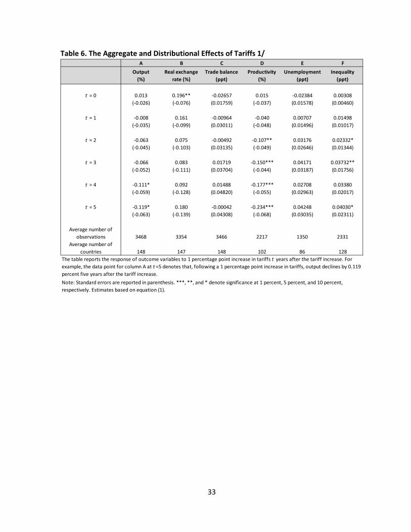
Table 6. The Aggregate and Distributional Effects of Tariffs 1/

A B C D E F

Output

(%)

Real exchange

rate (%)

Trade balance

(ppt)

Productivity

(%)

Unemployment

(ppt)

Inequality

(ppt)

t = 0 0.013 0.196** ‐0.02657 0.015 ‐0.02384 0.00308

(‐0.026) (‐0.076) (0.01759) (‐0.037) (0.01578) (0.00460)

t = 1 ‐0.008 0.161 ‐0.00964 ‐0.040 0.00707 0.01498

(‐0.035) (‐0.099) (0.03011) (‐0.048) (0.01496) (0.01017)

t = 2 ‐0.063 0.075 ‐0.00492 ‐0.107** 0.03176 0.02332*

(‐0.045) (‐0.103) (0.03135) (‐0.049) (0.02646) (0.01344)

t = 3 ‐0.066 0.083 0.01719 ‐0.150*** 0.04171 0.03732**

(‐0.052) (‐0.111) (0.03704) (‐0.044) (0.03187) (0.01756)

t = 4 ‐0.111* 0.092 0.01488 ‐0.177*** 0.02708 0.03380

(‐0.059) (‐0.128) (0.04820) (‐0.055) (0.02963) (0.02017)

t = 5 ‐0.119* 0.180 ‐0.00042 ‐0.234*** 0.04248 0.04030*

(‐0.063) (‐0.139) (0.04308) (‐0.068) (0.03035) (0.02311)

Average number of

observations 3468 3354 3466 2217 1350 2331

Average number of

countries 148 147 148 102 86 128

Note: Standard errors are reported in parenthesis. ***, **, and * denote significance at 1 percent, 5 percent, and 10 percent,

respectively. Estimates based on equation (1).

The table reports the response of outcome variables to 1 percentage point increase in tariffs t years after the tariff increase. For

example, the data point for column A at t =5 denotes that, following a 1 percentage point increase in tariffs, output declines by 0.119

percent five years after the tariff increase.

34

Figure 1. The Effect of Tariffs

Panel A. Output (%) Panel B. Productivity (%)

Panel C. Unemployment (ppt) Panel D. Inequality (ppt)

Panel E. Real exchange rate (%) Panel F. Trade balance‐to‐GDP ratio (ppt)

Note: The solid line indicates the response of output (real exchange rate, trade balance, labor productivity,

unemployment, inequality) to a one standard deviation increase in tariff; the dotted lines correspond to 90%

confidence bands. The x‐axis denotes time. t=0 is the year of the change. The estimates are based on equation

(1).

‐1.0

‐0.8

‐0.6

‐0.4

‐0.2

0.0

0.2

0.4

‐1 0 1 2 3 4 5

‐1.4

‐1.2

‐1

‐0.8

‐0.6

‐0.4

‐0.2

0

0.2

0.4

‐1 0 1 2 3 4 5

‐0.3

‐0.2

‐0.1

0

0.1

0.2

0.3

0.4

‐1 0 1 2 3 4 5

‐0.05

0

0.05

0.1

0.15

0.2

0.25

0.3

0.35

‐1 0 1 2 3 4 5

‐1.0

‐0.5

0.0

0.5

1.0

1.5

2.0

‐1 0 1 2 3 4 5

‐0.3

‐0.2

‐0.1

0

0.1

0.2

0.3

0.4

‐1 0 1 2 3 4 5

35

Figure 2. The Effect of Tariffs—Tariff Increases vs. Decreases; Advanced Economies vs.

Emerging Markets & Developing Economies

Output (%) Productivity (%)

Panel A. Tariff Increases

Panel B. Tariff Decreases

Panel C. Advanced Economics

Panel D. Emerging Markets & Developing Economies

Note: The solid black line indicates the response of output (productivity) to a one standard deviation increase

and decrease in tariff (advanced economies and emerging markets & developing economies); the dotted lines

correspond to 90% confidence bands; estimates for Panel A and B are based on equation (2); estimates for

Panel C and D are based on equation (3). Dashed red lines indicate the response of output (productivity) to a

one standard deviation increase in tariff in the baseline; estimates based on equation (1). The x‐axis denotes

time. t=0 is the year of the tariff change.

‐2.5

‐2.0

‐1.5

‐1.0

‐0.5

0.0

0.5

‐1 0 1 2 3 4 5

‐4

‐3

‐2

‐1

0

1

‐1 0 1 2 3 4 5

‐1.0

‐0.5

0.0

0.5

1.0

‐1 0 1 2 3 4 5

‐1

‐0.5

0

0.5

1

‐1 0 1 2 3 4 5

‐3.0

‐2.0

‐1.0

0.0

1.0

‐1 0 1 2 3 4 5

‐2.5

‐2

‐1.5

‐1

‐0.5

0

0.5

‐1 0 1 2 3 4 5

‐1.0

‐0.5

0.0

0.5

‐1 0 1 2 3 4 5

‐1.5

‐1

‐0.5

0

0.5

1

‐1 0 1 2 3 4 5

36

Figure 3. The Effect of Tariffs—Expansions vs. Recessions


Panel A. Expansions (based on GDP growth)

Panel B. Recessions (based on GDP growth)

Panel C. Expansions (based on unemployment changes)

Panel D. Recessions (based on unemployment changes)

Note: The solid black line indicates the response of output (productivity) to a one standard deviation increase

in tariff during expansions and recessions; the dotted lines correspond to 90% confidence bands; estimates

based on equation (4); for Panel A and B expansions and recessions are identified using GDP growth; for Panel

C and D using unemployment changes. Dashed red lines indicate the response of output (productivity) to a

one standard deviation increase in tariff in the baseline; estimates based on equation (1). The x‐axis denotes

time. t=0 is the year of the tariff change.

‐2.5

‐2.0

‐1.5

‐1.0

‐0.5

0.0

0.5

‐1 0 1 2 3 4 5

‐4

‐3

‐2

‐1

0

1

‐1 0 1 2 3 4 5

‐1.0

‐0.5

0.0

0.5

1.0

1.5

2.0

‐1 0 1 2 3 4 5

‐2

‐1

0

1

2

3

‐1 0 1 2 3 4 5

‐4.0

‐3.0

‐2.0

‐1.0

0.0

1.0

2.0

‐1 0 1 2 3 4 5

‐5

‐4

‐3

‐2

‐1

0

1

‐1 0 1 2 3 4 5

‐1.0

0.0

1.0

2.0

3.0

‐1 0 1 2 3 4 5

‐2

‐1

0

1

2

3

4

‐1 0 1 2 3 4 5

37

Figure 4. Robustness for Output

Default (Figure 1) Percent change of tariffs Lag tariffs

VAR‐style Include contemporary shocks Include growth forecasts

IV Drop series with gaps Drop high inflation (>100%)

Drop small population (<1million) Drop outliers Drop early years (<1980)

Drop high tariffs (>66 percent) Drop Americas Drop Asians/Africans

Note: The black solid line indicates the response of output to a one standard deviation increase in tariff using

the scenarios described in each title of the chart. The red dotted line represents the baseline results,

estimated based on equation (1). The blue dotted lines correspond to 90% confidence bands of the baseline.

The x‐axis denotes time. t=0 is the year of the change.

‐1.0

0.0

1.0

‐1 0 1 2 3 4 5

‐1.0

0.0

1.0

‐1 0 1 2 3 4 5

‐1.0

0.0

1.0

‐1 0 1 2 3 4 5

‐1.0

0.0

1.0

‐1 0 1 2 3 4 5

‐1.0

0.0

1.0

‐1 0 1 2 3 4 5

‐1.0

0.0

1.0

‐1 0 1 2 3 4 5

‐1.0

0.0

1.0

‐1 0 1 2 3 4 5‐1.0

0.0

1.0

‐1 0 1 2 3 4 5

‐1.0

0.0

1.0

‐1 0 1 2 3 4 5‐1.0

0.0

1.0

‐1 0 1 2 3 4 5

‐1.0

0.0

1.0

‐1 0 1 2 3 4 5

‐2.0

‐1.0

0.0

1.0

‐1 0 1 2 3 4 5

‐1.0

0.0

1.0

0 1 2 3 4 5

‐1.0

0.0

1.0

‐1 0 1 2 3 4 5

‐1.0

0.0

1.0

‐1 0 1 2 3 4 5

38

Figure 5. Robustness for Productivity






Note: The black solid line indicates the response of productivity to a one standard deviation increase in tariff

using the scenarios described in each title of the chart. The red dotted line represents the baseline results,



‐2

‐1

0

1

‐1 0 1 2 3 4 5

‐2

‐1

0

1

‐1 0 1 2 3 4 5

‐2

‐1

0

1

‐1 0 1 2 3 4 5

‐2

‐1

0

1

‐1 0 1 2 3 4 5

‐2

‐1

0

1

‐1 0 1 2 3 4 5

‐2

‐1

0

1

‐1 0 1 2 3 4 5

‐2

‐1

0

1

‐1 0 1 2 3 4 5‐2

‐1

0

1

‐1 0 1 2 3 4 5

‐2

‐1

0

1

‐1 0 1 2 3 4 5‐2

‐1

0

1

‐1 0 1 2 3 4 5

‐2

‐1

0

1

‐1 0 1 2 3 4 5

‐2

‐1

0

1

‐1 0 1 2 3 4 5

‐2

‐1

0

1

‐1 0 1 2 3 4 5

‐2

‐1

0

1

0 1 2 3 4 5

‐1.0

0.0

1.0

‐1 0 1 2 3 4 5

39

Figure 6. The Effect of Tariffs using Industry‐level Data


Panel A. The Effect of Input Tariffs

Panel B. The Effect of Output Tariffs

Note: The solid line indicates the response of output/labor productivity to a one standard deviation increase in

input/output tariff; the dotted lines correspond to 90% confidence bands. The x‐axis denotes time. t=0 is the

year of the change. The estimates are based on equation (1’).

‐12

‐10

‐8

‐6

‐4

‐2

0

2

4

‐1 0 1 2 3 4 5‐8

‐6

‐4

‐2

0

2

4

6

‐1 0 1 2 3 4 5

‐3

‐2

‐1

0

1

2

3

4

5

6

‐1 0 1 2 3 4 5

‐4

‐3

‐2

‐1

0

1

2

3

4

5

‐1 0 1 2 3 4 5

40

Appendix I—Three Episodes of Tariff Hikes

In this appendix, we briefly describe three cases where tariffs rose in our sample. Without

claiming these episodes represent all tariff variation, they seem typical to us. Tariffs rose in

Denmark mostly because of a foreign shock, in Colombia because of overshooting in the

foreign exchange market, and in India because of a war. In no case do domestic

macroeconomic considerations seem to be overwhelming; in all cases, the primary causes

seem wrapped up in the balance of payments.

Denmark 1971

Most advanced economies have tariffs that start relatively low and fall throughout most of

the sample period. But there are some exceptions. Denmark’s newly elected Social

Democratic government moved to impose a ten percent import surcharge on two‐thirds of

the country’s imports on its first day in office, Oct 19, 1971.* It was introduced to

strengthen the currency and improve the balance of payments before the country joined

the European Economic Community (the predecessor to the European Union) and was

explicitly limited in duration. This surcharge was a partial response to the “Nixon Shock” of

August 1971, which imposed a ten percent surcharge on all dutiable American imports,

intended to force a real American depreciation.† In our data set, the jump in Danish tariffs

shows up clearly:

Year Tariff

1971 7.3%

1972 12.0%

1973 12.8%

1974 11.0%

Colombia 1964

A number of developing countries experienced extreme protectionism, especially countries

pursuing import‐substitution strategies. But there are other causes; some of the

protectionist surges were triggered by balance of payments issues. In late 1964, the central

bank of Colombia floated the over‐valued exchange rate, which then depreciated

excessively, by almost 90%. Colombia then moved to protect its international reserves by

* https://www.nytimes.com/1971/10/20/archives/denmark-moved-quickly-on-surtax.html

† https://www.nytimes.com/1971/10/20/archives/denmark-plans-surcharge-as-protectionist-measure-european-trading.html

41

prohibiting the free import of almost all foreign products for a 90‐day period, pursued a

standby package with the IMF, and … raised tariffs.‡

Year Tariff

1961 31.5%

1962 49.8%

1963 47.3%

1964 70.4%

1965 55.3%

1966 36.1%

India 1972

Indian development post‐independence was guided by a series of five‐year plans. By the

fourth plan (covering 1969‐73), there was a deliberate attempt to steer the economy

towards self‐reliance through import‐substitution.§ As part of the plan, tariffs were

imposed on all goods other than grain and a few smaller exceptions. Still, the more

immediate reason for the protectionist spike was undoubtedly the Indo‐Pakistani war of

December 1971.

1969 59.4%

1970 58.7%

1971 63.8%

1972 91.4%

1973 76.2%

1974 64.9%

‡ https://www.nytimes.com/1964/12/02/archives/colombia‐curbs‐all‐free‐imports‐90day‐ban‐is‐imposedlatin‐

bloc.html; also see “The Political Economy of Exchange Rate Policy in Colombia” by Jaramillo, Steiner and

Salazar, IDB Working Paper No. 102, 1999.

§ http://shodhganga.inflibnet.ac.in/bitstream/10603/32033/14/14_chapter%208.pdf

42

APPENDIX II—RESULTS FOR UNEMPLOYMENT, INEQUALITY, REAL EXCHANGE RATE, AND TRADE BALANCE

Figure AII.1. The Effect of Tariffs—Tariff Increases vs. Decreases; Advanced Economies vs.


Unemployment (ppt) Inequality (ppt)





Note: The solid black line indicates the response of unemployment (inequality) to a one standard deviation increase and decrease in tariff

(advanced economies and emerging markets & developing economies); the dotted lines correspond to 90% confidence bands; estimates

for Panel A and B are based on equation (2); estimates for Panel C and D are based on equation (3). Dashed red lines indicate the response

of unemployment (inequality) to a one standard deviation increase in tariff in the baseline; estimates based on equation (1). The x‐axis

denotes time. t=0 is the year of the tariff change.

‐0.6‐0.4‐0.2

00.20.40.60.8

‐1 0 1 2 3 4 5

‐0.2‐0.1

00.10.20.30.40.5

‐1 0 1 2 3 4 5

‐0.4

‐0.2

0

0.2

0.4

0.6

‐1 0 1 2 3 4 5

‐0.1

0

0.1

0.2

0.3

0.4

‐1 0 1 2 3 4 5

‐1.5‐1

‐0.50

0.51

1.52

‐1 0 1 2 3 4 5

‐0.4

‐0.2

0

0.2

0.4

‐1 0 1 2 3 4 5

‐0.3‐0.2‐0.1

00.10.20.30.4

‐1 0 1 2 3 4 5

‐0.1

0

0.1

0.2

0.3

0.4

‐1 0 1 2 3 4 5

43

Figure AII.2. The Effect of Tariffs—Expansions vs. Recessions

Unemployment (%) Inequality (%)





Note: The solid black line indicates the response of unemployment (inequality) to a one standard deviation

increase in tariff during expansions and recessions; the dotted lines correspond to 90% confidence bands;

estimates based on equation (4); for Panel A and B expansions and recessions are identified using GDP growth;

for Panel C and D using unemployment changes. Dashed red lines indicate the response of unemployment

(inequality) to a one standard deviation increase in tariff in the baseline; estimates based on equation (1). The

x‐axis denotes time. t=0 is the year of the tariff change.

‐1

‐0.5

0

0.5

1

1.5

‐1 0 1 2 3 4 5

‐0.4

‐0.2

0

0.2

0.4

‐1 0 1 2 3 4 5

‐1

‐0.5

0

0.5

1

‐1 0 1 2 3 4 5

‐0.2

0

0.2

0.4

0.6

0.8

‐1 0 1 2 3 4 5

‐1

‐0.5

0

0.5

1

‐1 0 1 2 3 4 5

‐0.4

‐0.2

0

0.2

0.4

0.6

‐1 0 1 2 3 4 5

‐1

‐0.5

0

0.5

1

‐1 0 1 2 3 4 5

‐0.3

‐0.2

‐0.1

0

0.1

0.2

0.3

‐1 0 1 2 3 4 5

44

Figure AII.3. The Effect of Tariffs—Tariff Increases vs. Decreases; Advanced Economies vs.


Real exchange rate (%) Trade balance‐to‐GDP ratio (ppt)





Note: The solid black line indicates the response of real exchange rate (trade balance) to a one standard

deviation increase and decrease in tariff (advanced economies and emerging markets & developing

economies); the dotted lines correspond to 90% confidence bands; estimates for Panel A and B are based on

equation (2); estimates for Panel C and D are based on equation (3). Dashed red lines indicate the response of

real exchange rate (trade balance) to a one standard deviation increase in tariff in the baseline; estimates

based on equation (1). The x‐axis denotes time. t=0 is the year of the tariff change.

‐3.0

‐2.0

‐1.0

0.0

1.0

2.0

‐1 0 1 2 3 4 5

‐1

‐0.5

0

0.5

1

1.5

‐1 0 1 2 3 4 5

‐0.50.00.51.01.52.02.53.0

‐1 0 1 2 3 4 5

‐0.8

‐0.6

‐0.4

‐0.2

0

0.2

0.4

‐1 0 1 2 3 4 5

‐2.0

‐1.0

0.0

1.0

2.0

3.0

‐1 0 1 2 3 4 5

‐0.4

‐0.2

0

0.2

0.4

0.6

0.8

‐1 0 1 2 3 4 5

‐1.0

‐0.5

0.0

0.5

1.0

1.5

2.0

‐1 0 1 2 3 4 5

‐0.4

‐0.2

0

0.2

0.4

‐1 0 1 2 3 4 5

45

Figure AII.4. The Effect of Tariffs—Expansions vs. Recessions

Real exchange rate (%) Trade balance‐to‐GDP ratio (ppt)





Note: The solid black line indicates the response of real exchange rate (trade balance) to a one standard

deviation increase in tariff during expansions and recessions; the dotted lines correspond to 90% confidence

bands; estimates based on equation (4); for Panel A and B expansions and recessions are identified using GDP

growth; for Panel C and D using unemployment changes. Dashed red lines indicate the response of real

exchange rate (trade balance) to a one standard deviation increase in tariff in the baseline; estimates based on

equation (1). The x‐axis denotes time. t=0 is the year of the tariff change.

‐2.0

‐1.0

0.0

1.0

2.0

3.0

4.0

‐1 0 1 2 3 4 5

‐1

‐0.5

0

0.5

1

1.5

‐1 0 1 2 3 4 5

‐3.0

‐2.0

‐1.0

0.0

1.0

2.0

3.0

‐1 0 1 2 3 4 5

‐1.5

‐1

‐0.5

0

0.5

1

1.5

‐1 0 1 2 3 4 5

‐6.0

‐4.0

‐2.0

0.0

2.0

‐1 0 1 2 3 4 5

‐1

‐0.5

0

0.5

1

1.5

2

‐1 0 1 2 3 4 5

‐2.0

0.0

2.0

4.0

6.0

8.0

‐1 0 1 2 3 4 5

‐1.5

‐1

‐0.5

0

0.5

1

‐1 0 1 2 3 4 5

46

APPENDIX III—ROBUSTNESS RESULTS FOR UNEMPLOYMENT, INEQUALITY, REAL EXCHANGE RATE, AND TRADE

BALANCE

Figure AIII.1. Robustness for Unemployment






Note: The black solid line indicates the response of unemployment to a one standard deviation increase in tariff using the scenarios

described in each title of the chart. The red dotted line represents the baseline results, estimated based on equation (1). The blue dotted

lines correspond to 90% confidence bands of the baseline. The x‐axis denotes time. t=0 is the year of the change.

‐0.5

0

0.5

‐1 0 1 2 3 4 5

‐0.5

0

0.5

‐1 0 1 2 3 4 5

‐0.5

0

0.5

‐1 0 1 2 3 4 5

‐0.5

0

0.5

‐1 0 1 2 3 4 5

‐0.5

0

0.5

‐1 0 1 2 3 4 5

‐0.5

0

0.5

‐1 0 1 2 3 4 5

‐0.5

0

0.5

‐1 0 1 2 3 4 5

‐0.5

0

0.5

‐1 0 1 2 3 4 5

‐0.5

0

0.5

‐1 0 1 2 3 4 5

‐0.5

0

0.5

‐1 0 1 2 3 4 5

‐0.5

0

0.5

‐1 0 1 2 3 4 5

‐0.5

0

0.5

‐1 0 1 2 3 4 5

‐0.5

0

0.5

0 1 2 3 4 5

‐0.5

0

0.5

‐1 0 1 2 3 4 5

‐0.5

0

0.5

‐1 0 1 2 3 4 5

47

Figure AIII.2. Robustness for Inequality






Note: The black solid line indicates the response of inequality to a one standard deviation increase in tariff




‐0.2

0

0.2

0.4

‐1 0 1 2 3 4 5

‐0.2

0

0.2

0.4

‐1 0 1 2 3 4 5

‐0.2

0

0.2

0.4

‐1 0 1 2 3 4 5

‐0.2

0

0.2

0.4

‐1 0 1 2 3 4 5

‐0.2

0

0.2

0.4

‐1 0 1 2 3 4 5

‐0.2

0

0.2

0.4

‐1 0 1 2 3 4 5‐0.2

0

0.2

0.4

‐1 0 1 2 3 4 5

‐0.2

0

0.2

0.4

‐1 0 1 2 3 4 5

‐0.2

0

0.2

0.4

‐1 0 1 2 3 4 5

‐0.2

0

0.2

0.4

‐1 0 1 2 3 4 5

‐0.2

0

0.2

0.4

‐1 0 1 2 3 4 5

‐0.2

0

0.2

0.4

‐1 0 1 2 3 4 5

‐0.2

0

0.2

0.4

‐1 0 1 2 3 4 5

‐0.2

0

0.2

0.4

0 1 2 3 4 5

‐0.2

0

0.2

0.4

‐1 0 1 2 3 4 5

48

Figure AIII.3. Robustness for Real Exchange Rate






Note: The black solid line indicates the response of real exchange rate to a one standard deviation increase in

tariff using the scenarios described in each title of the chart. The red dotted line represents the baseline

results, estimated based on equation (1). The blue dotted lines correspond to 90% confidence bands of the

baseline. The x‐axis denotes time. t=0 is the year of the change.

‐2.0

0.0

2.0

‐1 0 1 2 3 4 5

‐2.0

0.0

2.0

‐1 0 1 2 3 4 5

‐2.0

0.0

2.0

‐1 0 1 2 3 4 5

‐2.0

0.0

2.0

‐1 0 1 2 3 4 5

‐2.0

0.0

2.0

‐1 0 1 2 3 4 5

‐2.0

0.0

2.0

‐1 0 1 2 3 4 5

‐2.0

0.0

2.0

‐1 0 1 2 3 4 5‐2.0

0.0

2.0

‐1 0 1 2 3 4 5

‐2.0

0.0

2.0

‐1 0 1 2 3 4 5‐2.0

0.0

2.0

‐1 0 1 2 3 4 5

‐2.0

0.0

2.0

‐1 0 1 2 3 4 5

‐5

0

5

‐1 0 1 2 3 4 5

‐2.0

0.0

2.0

0 1 2 3 4 5‐2.0

0.0

2.0

‐1 0 1 2 3 4 5

‐2.0

0.0

2.0

4.0

‐1 0 1 2 3 4 5

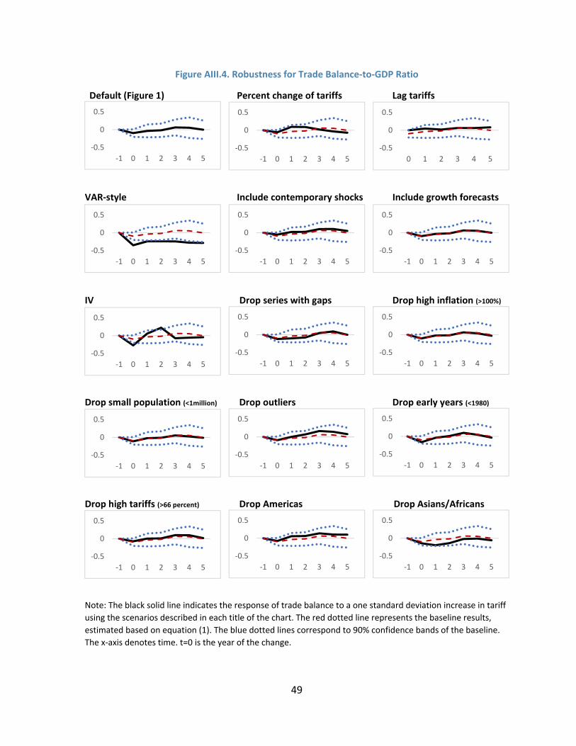
49

Figure AIII.4. Robustness for Trade Balance‐to‐GDP Ratio






Note: The black solid line indicates the response of trade balance to a one standard deviation increase in tariff




‐0.5

0

0.5

‐1 0 1 2 3 4 5

‐0.5

0

0.5

‐1 0 1 2 3 4 5

‐0.5

0

0.5

‐1 0 1 2 3 4 5

‐0.5

0

0.5

‐1 0 1 2 3 4 5

‐0.5

0

0.5

‐1 0 1 2 3 4 5

‐0.5

0

0.5

‐1 0 1 2 3 4 5

‐0.5

0

0.5

‐1 0 1 2 3 4 5

‐0.5

0

0.5

‐1 0 1 2 3 4 5

‐0.5

0

0.5

‐1 0 1 2 3 4 5

‐0.5

0

0.5

‐1 0 1 2 3 4 5

‐0.5

0

0.5

‐1 0 1 2 3 4 5

‐0.5

0

0.5

‐1 0 1 2 3 4 5

‐0.5

0

0.5

‐1 0 1 2 3 4 5

‐0.5

0

0.5

0 1 2 3 4 5

‐0.5

0

0.5

‐1 0 1 2 3 4 5

50

APPENDIX IV—RESULTS FOR CONSUMPTION AND INFLATION

Figure AIV.1: Baseline and Selected Asymmetric Results for Consumption and Inflation

Panel A: Baseline for Consumption Panel B: Baseline for Inflation

The Asymmetric Effect on Consumption

Panel C: Tariff Increases

Panel D: Tariff Decreases

The Asymmetric Effect on Inflation

Panel E: Expansions (based on GDP growth)

Panel F: Recessions (based on GDP growth)

Note: The solid black line indicates the response of consumption (inflation) to a one standard deviation increase in tariff;

the dotted lines correspond to 90% confidence bands; estimates for Panel A and B are based on equation (1); estimates for

Panel C and D are based on equation (2); estimates for Panel E and F are based on equation (4). Dashed red lines indicate

the response of consumption (inflation) to a one standard deviation increase in tariff in the baseline; estimates based on

equation (1). The x‐axis denotes time. t=0 is the year of the tariff change.

‐2.5

‐2

‐1.5

‐1

‐0.5

0

0.5

‐1 0 1 2 3 4 5

‐1

‐0.5

0

0.5

1

‐1 0 1 2 3 4 5

‐5.0

0.0

5.0

10.0

15.0

20.0

25.0

‐1 0 1 2 3 4 5

‐40.0

‐30.0

‐20.0

‐10.0

0.0

10.0

‐1 0 1 2 3 4 5

‐1.0

‐0.8

‐0.6

‐0.4

‐0.2

0.0

0.2

0.4

0.6

‐1 0 1 2 3 4 5

‐2

0

2

4

6

8

10

‐1 0 1 2 3 4 5

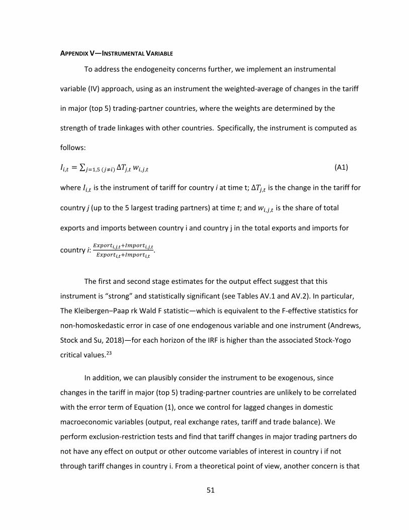
51

APPENDIX V—INSTRUMENTAL VARIABLE

To address the endogeneity concerns further, we implement an instrumental

variable (IV) approach, using as an instrument the weighted‐average of changes in the tariff

in major (top 5) trading‐partner countries, where the weights are determined by the

strength of trade linkages with other countries. Specifically, the instrument is computed as

follows:

𝐼 , ∑ ∆𝑇 ,, 𝑤 , , (A1)

where 𝐼 , is the instrument of tariff for country i at time t; ∆𝑇 , is the change in the tariff for

country j (up to the 5 largest trading partners) at time t; and 𝑤 , , is the share of total

exports and imports between country i and country j in the total exports and imports for

country i: , , , ,

, ,.

The first and second stage estimates for the output effect suggest that this

instrument is “strong” and statistically significant (see Tables AV.1 and AV.2). In particular,

The Kleibergen‒Paap rk Wald F statistic—which is equivalent to the F‐effective statistics for

non‐homoskedastic error in case of one endogenous variable and one instrument (Andrews,

Stock and Su, 2018)—for each horizon of the IRF is higher than the associated Stock‐Yogo

critical values.23

In addition, we can plausibly consider the instrument to be exogenous, since

changes in the tariff in major (top 5) trading‐partner countries are unlikely to be correlated

with the error term of Equation (1), once we control for lagged changes in domestic

macroeconomic variables (output, real exchange rates, tariff and trade balance). We

perform exclusion‐restriction tests and find that tariff changes in major trading partners do

not have any effect on output or other outcome variables of interest in country i if not

through tariff changes in country i. From a theoretical point of view, another concern is that

52

the instrument could be correlated with the error term to the extent that changes in tariff

rates in main large trading partners could affect domestic output through

contemporaneous changes in the real exchange rate. To address this issue, we modify the

equation to control for the contemporaneous changes in other control variables, including

the real exchange rates. The results are robust to this specification and very similar to those

presented in Figure 5.

Table AV.1. First Stage estimates of Change in Tariffs on the Instrument (the weighted‐

average of changes in the tariff in major (top 5) trading‐partner countries)

Instrument (t) 0.446***

(3.97)

Change in Tariff (t‐1) ‐0.160**

(‐9.79)

Change in Tariff (t‐2) ‐0.044***

(‐2.82)

Output growth (t‐1) ‐1.400

(‐0.94)

Output growth (t‐2) 0.585

(0.40)

Change in REER (t‐1) 0.001

90.09)

Change in REER (t‐2) 0.005

(0.58)

Change in Trade Balance (t‐1) 0.332

(0.64)

Change in Trade Balance (t‐2) 0.031

(0.06)

N 3717

R2 0.08 ***,**,denote significance at 1 and 5 percent, respectively.

53

Table AV.2. Second Stage estimates of Output on the Change in Tariff Instrumented

K=0 K=1 K=2 K=3 K=4 K=5

Change in Tariff_Instumented (t‐1) 0.503*

(1.78)

‐0.001

(‐0.00)

‐0.785

(‐1.07)

‐0.770

(‐1.29)

‐1.295**

(‐1.97)

‐1.235**

(‐1.97)

Change in Tariff (t‐1) 0.069

(1.37)

‐0.044

(‐0.60)

‐0.160

(‐1.53)

‐0.197**

(‐2.00)

‐0.280***

(‐2.45)

‐0.280***

(‐2.47)

Change in Tariff (t‐2) ‐0.011

(‐0.64)

‐0.036

(‐1.49)

‐0.106***

(‐2.71)

‐0.125***

(‐3.46)

‐0.144***

(‐4.09)

‐0.170***

(‐6.74)

Output growth (t‐1) 0.275***

(7.66)

0.329***

(8.94)

0.351***

(7.81)

0.332***

(5.34)

0.290***

(3.62)

0.277***

(3.06)

Output growth (t‐2) 0.005

(0.19)

0.035

(0.66)

0.017

(0.20)

‐0.007

(‐0.07)

‐0.026

(‐0.26)

‐0.025

(‐0.25)

Change in REER (t‐1) ‐0.028*

(‐1.82)

‐0.069***

(‐4.29)

‐0.099***

(‐4.59)

‐0.080**

(‐2.27)

‐0.038

(‐0.74)

‐0.013

(‐0.22)

Change in REER (t‐2) ‐0.027

(‐1.39)

‐0.055*

(‐1.75)

‐0.034

(‐0.69)

0.010

(0.15)

0.033

(0.42)

0.051

(0.68)

Change in Trade Balance (t‐1) ‐1.511**

(‐2.52)

‐2.749**

(‐2.43)

‐3.598*

(‐1.76)

‐3.611*

(‐1.86)

‐2.766*

(‐1.75)

‐1.814

(‐1.06)

Change in Trade Balance (t‐2) ‐1.001*

(‐1.84)

‐2.298**

(‐2.13)

‐2.221

(‐1.50)

‐1.231

(‐0.61)

‐0.013

(‐0.06)

1.472

(0.75)

N 3716 3622 3502 3387 3265 3145

KP F‐statistics

(Stock‐Yogo critical value 10%)

21.270

(16.38)

24.834

(16.38)

22.737

(16.38)

21.795

(16.38)

25.536

(16.38)

25.297

(16.38)

Note: t‐statistic based on Driscoll‐Kraay standard errors. ***,**,* denote significance at 1, 5 and 10 percent,

respectively. Instrument computed as the weighted‐average of changes in the tariff in major (top 5) trading‐

partner countries. Estimates based on equation (1).

54

Endnotes

1 For example, see the survey on free trade in Initiative on Global Markets (University of Chicago Booth School of Business): http://www.igmchicago.org/surveys/free‐trade. 2 If changes in tariffs are correlated with changes in non‐tariff barriers (NTBs), there may be a concern with omitted variable bias. To test this, we run panel regressions on the relationship between three different measures of NTBs (anti‐dumping cases initiated, safeguards, and WTO disputes) and changes in tariffs, controlling for country‐ and time‐fixed effects (as in our estimation framework described in equation 1). We do not find evidence of any strong correlation, mitigating this concern in our set‐up. However, the results should be taken with a pinch of salt since NTBs are difficult to measure and data is scarce for this exercise. 3 Kehoe (2003) compares the predictions of three ex‐ante CGE studies of NAFTA with observed outcomes and concludes that trade increases in most sectors surpassed the predictions more than ten‐fold. Corcos et. al (2012) find same results for the EU.

4 Since the set of control variables includes lags of output growth as well as the real exchange rate and trade balance, this approach is equivalent to a VAR approach in which tariff shocks do not respond to shocks in other variables within a year. We relax this assumption later as a robustness check.

5 While the original INDSTAT 2 database includes 23 manufacturing industries, exclude the “manufacture of recycling” industry due to insufficient observations.

6 The average and standard deviation of the change in the tariff rate in our sample are ‐0.4 and 3.6 percentage points, respectively. Tariff changes range from ‐52.0 to 41.0 percentage points. 7 Table 6 tabulates the underlying regression results.

8 Employment increases by about 0.5 percent but the effect is not statistically significant. 9 This result is consistent with evidence in Jaumotte, Lall and Papageorgiou (2013) who find that trade openness is associated with lower income inequality. While more work is needed to understand the distributional effects of tariffs, we believe that the increase in unemployment is a potentially important channel. Another possibility is that rent‐seeking means that protectionism benefits more the rich than the poor. 10 Using a multi‐country, multi‐sector, multi‐factor model of world production and trade with global input‐output linkages, Bonadio and Levchenko (2018) show that revoking NAFTA would reduce US welfare by about 0.2 percent, and Canadian and Mexican welfare by about 2 percent, with a real wage decline of 0.3 in the US and 1.7 in Canada and Mexico.

11 See Appendix I for some examples of major tariff increases in our sample. 12 Around 28 percent of our sample observations consist of tariff changes for advanced economies (with a mean of ‐.3 percentage points and standard deviation of 2.2) and 65 percent of the observations consist of tariff changes for other countries (with mean of ‐.3 and standard deviation of 4.1). While tariff changes have been less frequent in rich countries, the average magnitude of the changes is similar across the samples. Similarly, we do not observe significantly differences in the ratio of positive‐to‐negative changes between AEs (65 percent) and non‐AEs (75 percent).

55

13 This approach is equivalent to the smooth transition autoregressive model developed by Granger and Terävistra (1993). The results are robust different value of θ, and to substitute F(zit) with a dummy variable which takes value for F(zit) greater than 0.5.

14 In line with Rose (2013), we find no statistically significant correlation between changes in tariffs and the measure of state of economy used in the paper. In particular, the correlation between changes in tariffs and the smooth transition function 𝐹 𝑧 is ‐0.001.

15 See Figures in Appendix II for equivalent results for unemployment, inequality, real exchange rate and trade balance. 16 In addition to the robustness checks described in detail below, we run a version where the estimations include observations with trade balance between +/‐50 percent of GDP given some of the extreme movements in this variable. Our baseline results are robust to this specification. 17 Analogous results for the other variables of interest (unemployment, inequality, the real exchange rate and the trade balance) are reported in Figures AIII, 1‐4 of the Appendix III; they demonstrate the basic insensitivity of our baseline results.

18 Specifically, we control for contemporaneous changes in the trade balance and real exchange rate for the regressions on output, productivity, unemployment and inequality. For the regression on trade balance (real exchange rate) we control only for simultaneous changes in the real exchange rate (trade balance). 19 The results are robust to alternative orderings. 20 The Kleibergen‒Paap rk Wald F statistic for each horizon of the IRF is always higher than the associated Stock‐Yogo critical values. 21 Similar results are obtained when top and bottom 5th percentiles of the same distribution are considered. 22 The result that input tariffs have a more detrimental output effect than output tariffs is consistent with previous empirical work examining the effect of input and output tariffs at the macro (e.g., Ahn et al. 2016) and at the firm level (e.g. Amiti and Konings 2007). 23 Similar results are also obtained for productivity.

the macroeconomy after tariffs davide furceri, swarnali...

Documents