The Macroeconomic Effects of Interest on Reserves

Peter N. Ireland∗

Boston College and NBER

February 2011

Abstract

This paper uses a New Keynesian model with banks and deposits, calibrated tomatch the US economy, to study the macroeconomic effects of policies that pay intereston reserves. While their effects on output and inflation are small, these policies requireimportant adjustments in the way that the monetary authority manages the supplyof reserves, as liquidity effects vanish and households’ portfolio shifts increase banks’demand for reserves when short-term interest rates rise. Money and monetary policyremain linked in the long run, however, since policy actions that change the price levelmust change the supply of reserves proportionately.

JEL: E31, E32, E51, E52, E58.

∗Please address correspondence to: Peter N. Ireland, Boston College, Department of Economics, 140Commonwealth Avenue, Chestnut Hill, MA 02467-3859 USA. Tel: (617) 552-3687. Fax: (617) 552-2308.Email: peter.ireland@bc.edu. http://www2.bc.edu/peter-ireland. The opinions, findings, conclusions, andrecommendations expressed herein are my own and do not reflect those of the National Bureau of EconomicResearch.

1 Introduction

Slowly but surely over the three decades that have passed since the Federal Reserve’s “mon-

etarist experiment” of 1979 through 1982, the role of the monetary aggregates in both the

making and analysis of monetary policy has eroded. Bernanke’s (2006) historical account ex-

plains how and why Federal Reserve officials gradually deemphasized measures of the money

supply as targets and indicators for monetary policy over these years. Taylor’s (1993) highly

influential work shows that, instead, Federal Reserve policy beginning in the mid-1980s is de-

scribed quite well by a strikingly parsimonious rule for adjusting the short-term interest rate

in response to movements in output and inflation. Taylor’s insight has since been embedded

fully into theoretical analyses of monetary policy and its effects on the macroeconomy, which

now depict central bank policy as a rule for managing the short-term interest rate. Indeed,

textbook New Keynesian models such as Woodford’s (2003) and Gali’s (2008) typically make

no reference at all to any measure of the money supply, yet succeed nonetheless in providing

a complete and coherent description of the dynamics of output, inflation, and interest rates.

Still, as discussed by Ireland (2008) with reference to both practice and theory, the

central bank’s ability to manage short-term interest rates has rested, ultimately, on its

ability to control, mainly through open market purchases and sales of government bonds,

the quantity of reserves supplied to the banking system. Recently, however, Goodfriend

(2002), Ennis and Weinberg (2007), and Keister, Martin, and McAndrews (2008) have all

suggested that to some extent, even this last remaining role for a measure of money in the

monetary policymaking process can vanish when the central bank pays interest on reserves.

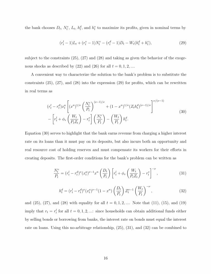
In the United States, interest on reserves moved quickly from being a theoretical possibility

to becoming an aspect of reality when, first, the Financial Services Regulatory Relief Act of

2006 promised to grant the Federal Reserve the power to pay interest on reserves starting

on October 1, 2011, second, the Emergency Economic Stabilization Act of 2008 brought

that starting date forward to October 1, 2008, and third, the Federal Reserve announced on

October 6, 2008 that it would, in fact, begin paying interest on reserves.

1

Figure 1 illustrates how the mechanics of the Federal Reserve’s federal funds rate targeting

procedures change with the introduction of interest payments on reserves. In each panel,

the quantity of reserves gets measured along the horizontal axis and the federal funds rate

along the vertical axis. Panel (a) depicts the traditional case, in which no interest is paid

on reserves. The demand curve for reserves slopes downward, since as the federal funds rate

falls those banks that typically borrow reserves find that the cost of doing so has declined

and those banks that typically lend reserves find that the benefit of doing so has declined: all

banks, therefore, wish to hold more reserves. The notation, DR(FFR;RR = 0, P0), makes

clear that while the demand curve describes a relationship between banks’ desired holdings

of reserves and the federal funds rate FFR, this relationship also depends on the fact that,

by assumption, the interest rate RR paid on reserves equals zero. Moreover, because reserves

are denominated in units of dollars, this relationship also depends on the aggregate price

level P0. In other words, a change in the federal funds rate leads to a movement along

the downward-sloping demand curve, whereas a change in either the interest rate paid on

reserves or the aggregate price level results in a shift in the demand curve.

Panel (a) therefore shows that with RR = 0 and the price level P0 taken as fixed in the

short run, the Federal Reserve hits its target FFR0 by conducting open market operations

that leave QR0 dollars of reserves to circulate among banks in the system. Panel (b) then

elaborates: if the Fed wants to lower its federal funds rate target from FFR0 to FFR1, it

must conduct an additional open market purchase of US Treasury securities that increases

the supply of reserves from QR0 to QR1. In this way, the Federal Reserve’s ability to manage

the short-term interest rate depends on its ability to control the supply of reserves as well.

Panel (c) of figure 1 then shows how the payment of interest on reserves places a floor

under the federal funds rate. For if the federal funds rate does fall below the rate RR0 at

which the Fed pays interest on reserves, any individual bank can earn profits by borrowing

reserves from another bank and depositing them at the Fed; this excess demand for reserves

then pushes the funds rate back to RR0. If there is a satiation point beyond which banks

2

will carry no more reserves, then the demand curve in panel (c) terminates when the funds

rate falls to RR0; if, instead, banks become willing to hold arbitrarily large stocks of reserves

when the opportunity cost of doing so falls to zero, then the demand curve flattens out

and follows the horizontal dotted line when the funds rate reaches RR0. Of course, these

observations simply generalize those that could have been made when describing panels (a)

and (b) for the case without interest on reserves: there, the lower bound for the federal funds

rate equals zero, since no bank will lend reserves at a negative interest rate when those funds

can be held without opportunity cost either as vault cash or as deposits at the Fed.

When, as in panel (c), the Federal Reserve’s funds rate target FFR0 lies above the interest

rate RR0 paid on reserves, the Fed must still conduct open market operations to make the

quantity of reserves supplied, QR2, equal to the quantity demanded. But, with interest on

reserves, the level of reserves QR2 required to support the funds rate target FFR0 in panel

(c) differs from the level of reserves QR0 required to support the same funds rate target shown

in panel (a) for the case without interest on reserves. This is one of the points emphasized by

Goodfried (2002), Ennis and Weinberg (2007), and Keister, Martin, and McAndrews (2008):

the authority to pay interest on reserves gives the Federal Reserve an additional tool of

monetary policy that provides another degree of freedom in the policymaking process since,

by adjusting the interest rate paid on reserves, the Fed can achieve different combinations

of settings for both the federal funds rate and the quantity of reserves.

Panel (d) of figure 1 highlights another manifestation of this same basic phenomenon.

If the Fed holds the interest rate it pays on reserves fixed at RR0, it must still conduct an

open market operation, changing the supply of reserves, to support a change in its federal

funds rate target; this remains exactly as before, in panel (b), where the interest rate on

reserves is also held fixed, more specifically, at zero. But suppose instead, as shown in

panel (d), that the Fed lowers both its funds rate target and the interest rate it pays on

reserves, so as to maintain a constant spread between the two. In this case, the lower rate

RR1 on reserves shifts the demand curve for reserves downward and to the left. A new

3

short-run equilibrium is established at the new funds rate target FFR1 without any change

in the quantity of reserves. To use Keister, Martin, and McAndrews’ (2008) apt words,

paying interest on reserves works to “divorce money” (meaning the quantity of reserves)

from “monetary policy” (meaning the federal funds rate).

Importantly, however, panels (a)-(d) hold other determinants of the demand for reserves

fixed. And, in particular, while the Keynesian assumption of a fixed aggregate price level

may be perfectly justified when looking at the effects of monetary policy actions over short

horizons, measured in days or weeks, the question remains as to what will happen over

longer intervals, as weeks blend into months and then quarter years and prices begin to

change. Going back to panels (a) and (b) for the case without interest on reserves, one

possibility is that the Fed simply reverses its policy action, using open market sales of US

Treasury securities it purchased previously to drain reserves from the banking system and

restore the initial equilibrium in which the funds rate rises again to FFR0 and the quantity

of reserves falls back to QR0. Another possibility, though, arises when the Fed leaves the

supply of reserves at the new, higher level QR1. The fractional reserve banking system will

then use these additional reserves to make new loans and create additional deposits. Broader

measures of the money supply will rise and, in the long run, will be matched by a rise in

prices that shifts the demand curve for reserves to the right as shown in panel (e). To avoid

dynamic instability, the Fed will have to allow the funds rate to return to its initial, higher

level FFR0. In this case, the monetary expansion has all of its classic effects: it decreases

interest rates and increases the money supply and output in the short run, but leaves interest

rates and output unchanged while increasing money and prices in the long run.

Going back to panels (c) and (d) for the case with interest on reserves, again one pos-

sibility is that the Federal Reserve reverses its initial actions, raising both its federal funds

rate target and the interest rate it pays on reserves so that the initial equilibrium gets re-

stored without a change in prices. Suppose, however, that the Fed holds interest rates low

enough, long enough, so that prices begin to rise. In panel (f), the rising price level shifts the

4

demand curve for reserves back to the right. To maintain an equilibrium and avoid dynamic

instability, it appears that the Fed must now do two things: raise its target for the funds

rate back to FFR0 and use open market operations to accommodate the increased demand

for reserves brought about by the rising price level. And if, in addition, the Fed wants to

maintain a constant spread between the funds rate and the interest rate it pays on reserves,

it will of course have to return the interest rate on reserves back to its original setting RR0 as

well. This last example reveals that, even with interest on reserves, monetary policy actions

that have macroeconomic effects, changing prices in the long run, still require open market

operations that change the quantity of reserves and the broader monetary aggregates. In

this example, money and monetary policy get divorced in the short run, but appear happily

reunited by the story’s close.

Above all, however, the series of examples considered in figure 1 illustrates how tricky it

can be to think about the dynamic effects of monetary policy using diagrams that hold many

endogenous variables fixed. Although, in several cases, the interest rate on reserves and even

the aggregate price level are allowed to vary together with the federal funds rate and the

quantity of reserves, all of the graphs ignore the effects that changes in output, brought about

by changes in monetary policy, have on the demand for reserves. Likewise, to the extent that

changes in the interest rate paid on reserves get passed along to consumers through changes

in retail deposit rates, and to the extent that changes in deposit rates then set off portfolio

rebalancing among households, additional effects that feed back into banks’ demand for

reserves get ignored as well. One cannot tell from these graphs whether changes in the federal

funds rate, holding the interest rate on reserves fixed either at zero or some positive rate,

have different effects on output and inflation than changes in the federal funds rate that occur

when the interest rate on reserves is moved in lockstep to maintain a constant spread between

the two; if that spread between the federal funds rate and the interest rate on reserves acts

as a tax on banking activity, those differences may be important too. Finally, it is of course

impossible to say much about the dynamic stability or instability of equilibria under different

5

monetary policymaking strategies with these two-dimensional diagrams. Assessing the full,

dynamic macroeconomic effects of monetary policies that involve the payment of interest on

reserves requires a fully dynamic and stochastic macroeconomic model. The purpose of this

paper is to build and analyze such a model, so as to explore the macroeconomic effects of

interest on reserves in more detail.

In previous work, Sargent and Wallace (1985) and Smith (1991) use overlapping gen-

erations models of money to see whether the payment of interest on reserves gives rise to

problems of equilibrium indeterminacy; here, these same issues are revisited, but with the

help of a New Keynesian model that resembles more closely the newer, textbook models of

Woodford (2003) and Gali (2008). Berentsen and Monnet (2008) also use a dynamic, general

equilibrium model to investigate the workings of monetary policy systems that pay interest

on reserves. In particular, Berentsen and Monnet employ a search-theoretic framework that

highlights, in great detail, how schemes involving the payment of interest on reserves can

make systems of payment operate more efficiently and thereby improve resource allocations

supported by decentralized markets in which money serves as a medium of exchange. Here,

as in Belongia and Ireland (2010) but in contrast to most other New Keynesian models, the

medium of exchange role played by currency and bank deposits receives some attention. But,

by generating a demand for money through a more stylized shopping-time specification as

opposed to an explicit description of decentralized trade, the model used here can go beyond

Berentsen and Monnet’s in other ways, allowing for a more detailed analysis of the dynamics

of macroeconomic variables including output, inflation, and interest rates that compares to

similar analyses conducted with more conventional New Keynesian models.

Finally and most recently, Kashyap and Stein (2010) develop a detailed model of the

financial sector, in which the spread between the federal funds rate and the interest rate

paid on reserves acts as a time-varying tax, and show how a central bank can use this time-

varying tax to optimally stabilize a fractional reserve banking system. Here, the spread

between the federal funds rate and the interest rate paid on reserves also gets modeled like

6

a tax on banks. Once again, however, the description of the banking system provided here

remains more stylized so that, while some attention is paid below to shocks that destabilize

the financial sector, issues relating to the optimal design, structure, and regulation of the

financial system cannot receive the very detailed consideration that they get in Kashyap and

Stein (2010) and the three other studies mentioned previously: Goodfriend (2002), Ennis

and Weinberg (2007), and Keister, Martin, and McAndrews (2008). Here, however, banks’

activities get modeled together with those of all other households and firms in the economy,

so that the broader focus can be on the macroeconomic effects of interest on reserves.

2 The Model

2.1 Overview

Belongia and Ireland (2010) extend the standard New Keynesian framework, exposited by

Woodford (2003) and Gali (2008) and used by many others, to incorporate roles for currency

and bank deposits in providing monetary services to households. There, the objective is to

revisit issues first raised by Barnett (1980) concerning the ability of simple-sum versus Divisia

monetary aggregates to track movements in the true quantity of monetary services provided

by liquid assets supplied by both the government and the private banking system. Here, the

same model gets extended still further to consider the macroeconomic effects of monetary

policies that manage both a short-term market rate of interest, like the federal funds rate

in the United States, and the rate of interest on reserves. This extended model allows the

host of issues, raised above with the help of figure 1, to be addressed head on, directly and

fully, with a dynamic, stochastic general equilibrium model, but requires a somewhat more

elaborate description of how banks optimally manage their holdings of reserves; the previous

model in Belongia and Ireland (2010) simply posits an exogenously-varying reserve ratio that

affects other aspects of bank behavior but it not itself an explicit choice variable as it is here.

The model economy consists of a representative consumer, a representative finished

7

goods-producing firm, a continuum of intermediate goods-producing firms indexed by i ∈

[0, 1], a representative bank, and a monetary authority. During each period t = 0, 1, 2, ...,

each intermediate goods-producing firm produces a distinct, perishable intermediate good.

Hence, the intermediate goods may also be indexed by i ∈ [0, 1], where firm i produces good

i. The model features enough symmetry, however, to allow the analysis to focus on the

behavior of a representative intermediate goods-producing firm that produces the generic

intermediate good i. The activities of each of these agents will now be described in turn.

2.2 The Representative Household

The representative household enters each period t = 0, 1, 2, ... with Mt−1 units of currency,

Bt−1 bonds, and st−1(i) shares in each intermediate goods-producing firm i ∈ [0, 1]. At the

beginning of the period, the household receives Tt additional units of currency in the form

of a lump-sum transfer from the monetary authority. Next, the households bonds mature,

providing Bt−1 more units of currency. The household uses some of this currency to purchase

Bt new bonds at the price of 1/rt dollars per bond, where rt denotes the gross nominal interest

rate between t and t + 1, and st(i) new shares in each intermediate goods-producing firm

i ∈ [0, 1] at the price of Qt(i) dollars per share.

After this initial securities-trading session, the household is left with

Mt−1 + Tt +Bt−1 +

∫ 1

0

Qt(i)st−1(i) di−Bt/rt −∫ 1

0

Qt(i)st(i) di

units of currency. It keeps Nt units of this currency to purchase goods and deposits the rest

in the representative bank. At the same time, the household also borrows Lt dollars from

the bank, bringing the total nominal value of its deposits to

Dt = Mt−1 + Tt +Bt−1 +

∫ 1

0

Qt(i)st−1(i) di−Bt/rt −∫ 1

0

Qt(i)st(i) di−Nt + Lt. (1)

During period t, the household supplies hgt (i) units of labor to each intermediate goods-

8

producing firm i ∈ [0, 1], for a total of

hgt =

∫ 1

0

hgt (i) di.

The household also supplies hbt units of labor to the representative bank. The household

therefore receives Wtht in labor income, where Wt denotes the nominal wage rate and ht =

hgt + hbt denotes total hours worked in goods production and banking.

Also during period t, the household purchase Ct units of the finished good at the nominal

price Pt from the representative finished goods-producing firm. Making this transaction

requires

hst =1

χ

(vat PtCtMa

t

)χ(2)

units of shopping time, where Mat is an aggregate of monetary services provided from cur-

rency Nt and deposits Dt according to

Mat = [(vn)1/ωN

(ω−1)/ωt + (1− vn)1/ωD

(ω−1)/ωt ]ω/(ω−1). (3)

In the shopping-time specification (2), the parameter χ > 1 governs the rate at which the

effort required to purchase goods and services increases as the household economizes on

its holdings of monetary assets. The shock vat impacts on the total demand for monetary

services; it follows the autoregressive process

ln(vat ) = (1− ρav) ln(va) + ρav ln(vat−1) + εavt, (4)

where va > 0 helps determine the steady-state level of real monetary services demanded

relative to consumption, the persistence parameter satisfies 0 ≤ ρav < 1, and the serially

uncorrelated innovation εavt has mean zero and standard deviation σav . In the monetary

aggregation specification (3), the parameter ω > 0 measures the elasticity of substitution

between currency and deposits in creating liquidity services and the parameter vn, satisfying

9

0 < vn < 1, helps determine the steady-state share of currency versus deposits in creating

the monetary aggregate.

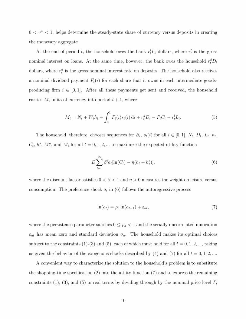
At the end of period t, the household owes the bank rltLt dollars, where rlt is the gross

nominal interest on loans. At the same time, however, the bank owes the household rdtDt

dollars, where rdt is the gross nominal interest rate on deposits. The household also receives

a nominal dividend payment Ft(i) for each share that it owns in each intermediate goods-

producing firm i ∈ [0, 1]. After all these payments get sent and received, the household

carries Mt units of currency into period t+ 1, where

Mt = Nt +Wtht +

∫ 1

0

Ft(i)st(i) di+ rdtDt − PtCt − rltLt. (5)

The household, therefore, chooses sequences for Bt, st(i) for all i ∈ [0, 1], Nt, Dt, Lt, ht,

Ct, hst , M

at , and Mt for all t = 0, 1, 2, ... to maximize the expected utility function

E∞∑t=0

βtat[ln(Ct)− η(ht + hst)], (6)

where the discount factor satisfies 0 < β < 1 and η > 0 measures the weight on leisure versus

consumption. The preference shock at in (6) follows the autoregressive process

ln(at) = ρa ln(at−1) + εat, (7)

where the persistence parameter satisfies 0 ≤ ρa < 1 and the serially uncorrelated innovation

εat has mean zero and standard deviation σa. The household makes its optimal choices

subject to the constraints (1)-(3) and (5), each of which must hold for all t = 0, 1, 2, ..., taking

as given the behavior of the exogenous shocks described by (4) and (7) for all t = 0, 1, 2, ....

A convenient way to characterize the solution to the household’s problem is to substitute

the shopping-time specification (2) into the utility function (7) and to express the remaining

constraints (1), (3), and (5) in real terms by dividing through by the nominal price level Pt

10

to obtain

Mt−1 + Tt +Bt−1 −Bt/rt −Nt + LtPt

+

∫ 1

0

[Qt(i)

Pt

][st−1(i)− st(i)] di ≥ Dt

Pt, (8)

[(vn)1/ω

(Nt

Pt

)(ω−1)/ω

+ (1− vn)1/ω(Dt

Pt

)(ω−1)/ω]ω/(ω−1)

≥ Mat

Pt, (9)

and

Nt +Wtht + rdtDt

Pt+

∫ 1

0

[Ft(i)

Pt

]st(i) di ≥ Ct +

rltLt +Mt

Pt, (10)

after allowing for free disposal. Letting Λ1t , Λ2

t , and Λ3t denote the nonnegative Lagrange

multipliers on these three constraints, the first-order conditions for the household’s problem

can be written as

Λ1t

rt= βEt

(Λ1t+1PtPt+1

), (11)

Λ1t

[Qt(i)

Pt

]= Λ3

t

[Ft(i)

Pt

]+ βEt

{Λ1t+1

[Qt+1(i)

Pt+1

]}(12)

for all i ∈ [0, 1],

Nt

Pt= vn

(Ma

t

Pt

)(Λ2t

Λ1t − Λ3

t

)ω, (13)

Dt

Pt= (1− vn)

(Ma

t

Pt

)(Λ2t

Λ1t − rdtΛ3

t

)ω, (14)

Λ1t = rltΛ

3t , (15)

ηat = Λ3t

(Wt

Pt

), (16)

atCt

[1− η

(vat PtCtMa

t

)χ]= Λ3

t , (17)

ηat

(vat PtCtMa

t

)χ= Λ2

t

(Ma

t

Pt

), (18)

and

Λ3t = βEt

(Λ1t+1PtPt+1

), (19)

11

together with (2) and (8)-(10) with equality for all t = 0, 1, 2, .... The implications of

these optimality conditions for issues relating to monetary aggregation and the demand for

monetary assets are discussed below.

2.3 The Representative Finished Goods-Producing Firm

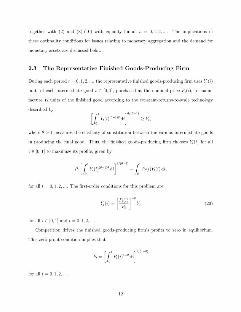
During each period t = 0, 1, 2, ..., the representative finished goods-producing firm uses Yt(i)

units of each intermediate good i ∈ [0, 1], purchased at the nominal price Pt(i), to manu-

facture Yt units of the finished good according to the constant-returns-to-scale technology

described by [∫ 1

0

Yt(i)(θ−1)θ di

]θ/(θ−1)≥ Yt,

where θ > 1 measures the elasticity of substitution between the various intermediate goods

in producing the final good. Thus, the finished goods-producing firm chooses Yt(i) for all

i ∈ [0, 1] to maximize its profits, given by

Pt

[∫ 1

0

Yt(i)(θ−1)θ di

]θ/(θ−1)−∫ 1

0

Pt(i)Yt(i) di,

for all t = 0, 1, 2, .... The first-order conditions for this problem are

Yt(i) =

[Pt(i)

Pt

]−θYt (20)

for all i ∈ [0, 1] and t = 0, 1, 2, ....

Competition drives the finished goods-producing firm’s profits to zero in equilibrium.

This zero profit condition implies that

Pt =

[∫ 1

0

Pt(i)1−θ di

]1/(1−θ)

for all t = 0, 1, 2, ....

12

2.4 The Representative Intermediate Goods-Producing Firm

During each period t = 0, 1, 2, ..., the representative intermediate goods-producing firm hires

hgt (i) units of labor from the representative household to manufacture Yt(i) units of interme-

diate good i according to the constant-returns-to-scale technology described by

Zthgt (i) ≥ Yt(i). (21)

The aggregate technology shock follows a random walk with positive drift:

ln(Zt) = ln(z) + ln(Zt−1) + εzt, (22)

where z > 1 and the serially uncorrelated innovation εzt has mean zero and standard devia-

tion σz.

Since the intermediate goods substitute imperfectly for one another in producing the

finished good, the representative intermediate goods-producing firm sells its output in a mo-

nopolistically competitive market. Hence, during each period t = 0, 1, 2, ..., the intermediate

goods-producing firm sets the nominal price Pt(i) for its output, subject to the require-

ment that it satisfy the representative finished goods-producing firm’s demand, described by

(20). In addition, following Rotemberg (1982), the intermediate goods-producing firm faces

a quadratic cost of adjusting its nominal price, measured in units of the finished good and

given by

φp2

[Pt(i)

πPt−1(i)− 1

]2Yt,

where the parameter φp > 0 governs the magnitude of the price adjustment cost and where

π > 1 denotes the gross, steady-state inflation rate.

The cost of price adjustment makes the intermediate goods-producing firm’s problem

dynamic: the firm chooses a sequence for Pt(i) for all t = 0, 1, 2, ... to maximize its total,

real market value, which from the equity-pricing relation (12) implied by the household’s

13

optimizing behavior is proportional to

E∞∑t=0

βtΛ3t

[Ft(i)

Pt

]

where

Ft(i)

Pt=

[Pt(i)

Pt

]1−θYt −

[Pt(i)

Pt

]−θ (WtYtPtZt

)− φp

2

[Pt(i)

πPt−1(i)− 1

]2Yt (23)

for all t = 0, 1, 2, .... The first-order conditions for this problem are

0 = (1− θ)Λ3t

[Pt(i)

Pt

]−θYt + θΛ3

t

[Pt(i)

Pt

]−θ−1(WtYtPtZt

)− φpΛ3

t

[Pt(i)

πPt−1(i)− 1

] [YtPt

πPt−1(i)

]+ βφpEt

{Λ3t+1

[Pt+1(i)

πPt(i)− 1

] [Yt+1Pt+1(i)Pt

πPt(i)2

]} (24)

for all t = 0, 1, 2, ....

2.5 The Representative Bank

During each period t = 0, 1, 2, ..., the representative bank accepts deposits worth Dt dollars

from the representative household. Creating these deposits requires N vt dollars in reserves

and hdt units of labor, where

xat

[(xn)1/ν

(N vt

Pt

)(ν−1)/ν

+ (1− xn)1/ν(Zthdt )

(ν−1)/ν

]ν/(ν−1)≥ Dt

Pt. (25)

In (25), the parameter ν > 0 measures the elasticity of substitution between reserves and

labor in the deposit creation process and the parameter xn, satisfying 0 < xn < 1, helps

determine the share of reserves relative to labor in producing deposits. The shock xat to

productivity in the banking sector follows the autoregressive process

ln(xat ) = (1− ρax) ln(xa) + ρax ln(xat−1) + εaxt, (26)

14

where xa > 0, 0 ≤ ρax < 1, and the serially uncorrelated innovation εaxt has mean zero and

standard deviation σax. In addition, to manage its stock of reserves worth N vt /Pt in real

terms, the bank must hire hvt additional units of labor, where

Zthvt ≥ φv

(N vt

Pt

). (27)

When the parameter φv > 0 is very small but still strictly positive, the additional labor

requirement embedded into the specification through (27) has little effect on real resource al-

locations, but ensures that banks’ holdings of reserves remain finite and uniquely-determined

even when the central bank pays interest on those reserves at a rate that equals the market

rate rt on bonds. This model feature thereby eliminates one potential source of equilibrium

indeterminacy by invoking the plausible assumption that looking after a larger stock of re-

serves always requires at least a small amount of additional time and effort from a bank’s

funds manager; the same assumption would make the demand curves for reserves in the

various panels of figure 1 terminate at the point where the federal funds rate falls to the rate

of interest paid on reserves, instead of extending infinitely far out, parallel to the horizon-

tal axis. Also, the assumption, reflected in both (25) and (27), that labor productivity in

banking activities grows at the same stochastic rate as it does in the production of interme-

diate goods as described by (21) and (22), ensures that the model remains consistent with

balanced growth.

After deciding on its optimal holding of reserves N vt , the bank lends out its remainin

funds Lt; its balance sheet constraint requires that

Dt

Pt≥ N v

t + LtPt

(28)

As noted above, deposits pay interest at the gross rate rdt and loans earn interest at the gross

rate rlt; in addition, reserves earn interest at the gross rate rvt . Hence, during each period t,

15

the bank chooses Dt, Nvt , Lt, h

dt , and hvt to maximize its profits, given in nominal terms by

(rlt − 1)Lt + (rvt − 1)N vt − (rdt − 1)Dt −Wt(h

dt + hvt ), (29)

subject to the constraints (25), (27) and (28) and taking as given the behavior of the exoge-

nous shocks as described by (22) and (26) for all t = 0, 1, 2, ....

A convenient way to characterize the solution to the bank’s problem is to substitute the

constraints (25), (27), and (28) into the expression (29) for profits, which can be rewritten

in real terms as

(rlt − rdt )xat

[(xn)1/ν

(N vt

Pt

)(ν−1)/ν

+ (1− xn)1/ν(Zthdt )

(ν−1)/ν

]ν/(ν−1)−[rlt + φv

(Wt

PtZt

)− rvt

](N vt

Pt

)−(Wt

Pt

)hdt .

(30)

Equation (30) serves to highlight that the bank earns revenue from charging a higher interest

rate on its loans than it must pay on its deposits, but also incurs both an opportunity and

real resource cost of holding reserves and must compensate its workers for their efforts in

creating deposits. The first-order conditions for the bank’s problem can be written as

N vt

Pt= (rlt − rdt )ν(xat )ν−1xn

(Dt

Pt

)[rlt + φv

(Wt

PtZt

)− rvt

]−ν, (31)

hdt = (rlt − rdt )ν(xat )ν−1(1− xn)

(Dt

Pt

)Zν−1t

(Wt

Pt

)−ν, (32)

and (25), (27), and (28) with equality for all t = 0, 1, 2, .... Note that (11), (15), and (19)

imply that rt = rlt for all t = 0, 1, 2, ...: since households can obtain additional funds either

by selling bonds or borrowing from banks, the interest rate on bonds must equal the interest

rate on loans. Using this no-arbitrage relationship, (25), (31), and (32) can be combined to

16

obtain

rdt = rt −1

xat

{xn[rt + φv

(Wt

PtZt

)− rvt

]1−ν+ (1− xn)

(Wt

PtZt

)1−ν}1/(1−ν)

, (33)

which shows how the cost of deposit creation, which in turn depends on the opportunity cost

of holding reserves and the cost of labor, causes the competitively-determined interest rate

on deposits to fall short of the interest rate on bonds and loans.

2.6 The Monetary Authority

As usual in New Keynesian models like this one, the central bank will be assumed to con-

duct monetary policy by adjusting the short-term market rate of interest rt in response to

movements in inflation πt = Pt/Pt−1 and a stationary measure of real economic activity, in

this case the rate of output growth

gt = Yt/Yt−1, (34)

since the level of output inherits a random walk from the nonstationary technology shock

(22). The modified Taylor (1993) rule

ln(rt/r) = ρr ln(rt−1/r) + ρπ ln(πt−1/π) + ρg ln(gt−1/g) + εrt (35)

allows, in addition, for interest rate smoothing through the lagged interest rate term on the

right-hand side. In (35), the constants r, π, and g denote the steady-state values of the

short-term nominal interest rate, the inflation rate, and the output growth rate, the Taylor

rule coefficients ρr ≥ 0, ρπ ≥ 0, and ρg ≥ 0 are chosen by the central bank, and the serially

uncorrelated innovation εrt has mean zero and standard deviation σr.

In addition, here, the central bank must also choose a rule for determining the interest

17

rate rvt it pays on reserves. By specifying a general rule of the form rvt = τtrαt or, in logs,

ln(rvt ) = ln(τt) + α ln(rt), (36)

where α ≥ 0 is a parameter, the new variable τt follows the autoregressive process

ln(τt) = (1− ρτ ) ln(τ) + ρτ ln(τt−1) + ετt (37)

with τ ≥ 1, 0 ≤ ρτ < 1, and the serially uncorrelated innovation ετt has mean zero and stan-

dard deviation στ , the general model allows flexibly for a number of special cases, including:

(i) the standard case α = 0, τ = 1, ρτ = 0, and στ = 0 in which no interest is paid on

reserves, (ii) the case α = 0, τ > 1, ρτ = 0, and στ = 0 in which interest is paid on reserves

at the constant, gross rate τ , (iii) the case α = 1, 0 < τ < 1, ρτ = 0, and στ = 0 depicted in

panels (c), (d), and (f) of figure 1 in which there is a constant, 100(1− τ) percentage-point

spread between the market rate and the interest rate on reserves, (iv) the case α = 1, τ = 1,

ρτ = 0, and στ = 0 in which interest is paid on reserves at the market rate, and (v) a variety

of cases with 0 ≤ ρτ < 1 and στ > 0 in which there is independent, stochastic variation in

the rate of interest on reserves, giving rise to a time-varying spread between the market rate

and the rate of interest on reserves.

2.7 Monetary Aggregation

In this model with currency and deposits, the variable Mat represents the true aggregate

of monetary services demanded by the representative household during each period t =

0, 1, 2, .... Note that (11) and (19), describing the representative household’s optimizing

behavior, imply that

Λ1t = rtΛ

3t (38)

18

for all t = 0, 1, 2, .... Substituting (38), together with (13) and (14), into (9) then yields

Λ2t

Λ3t

= [vn(rt − 1)1−ω + (1− vn)(rt − rdt )(1−ω)]1/(1−ω). (39)

Define the own rate of return rat on the monetary aggregate Mat with reference to the right-

hand side of (39):

rt − rat = [vn(rt − 1)1−ω + (1− vn)(rt − rdt )(1−ω)]1/(1−ω). (40)

Then one can verify that if the household’s choices of currency and deposits are not of

independent interest, the household’s problem can be stated more simply as one of choosing

sequences for Bt, st(i) for all i ∈ [0, 1], Lt, ht, Ct, Mat , and Mt for all t = 0, 1, 2, ... to

maximize the expected utility function obtained by substituting (2) into (6) subject to the

constraints

Mt−1 + Tt +Bt−1 −Bt/rt + LtPt

+

∫ 1

0

[Qt(i)

Pt

][st−1(i)− st(i)] di ≥ Ma

t

Pt,

and

Wtht + ratMat

Pt+

∫ 1

0

[Ft(i)

Pt

]st(i) di ≥ Ct +

rltLt +Mt

Pt

for all t = 0, 1, 2, ..., confirming that Mat represents a true economic aggregate of monetary

services.

Equations (38)-(40) also allow (16) and (18) to be combined to obtain

ln

(Ma

t

Pt

)=

χ

1 + χln(Ct) +

1

1 + χln

(Wt

Pt

)− 1

1 + χln(rt − rat ) +

χ

1 + χln(vat ), (41)

and (13) and (14) to be rewritten as

Nt

Pt= vn

(uatunt

)ω (Ma

t

Pt

)(42)

19

and

Dt

Pt= (1− vn)

(uatudt

)ω (Ma

t

Pt

), (43)

where

uat =rt − ratrt

, (44)

unt =rt − 1

rt, (45)

and

udt =rt − rdtrt

, (46)

use Barnett’s (1978) formula to define the user costs uat , unt , and udt of the monetary aggregate

Mat , currency Nt, and deposits Dt. Equation (41) takes the form of a demand curve for

monetary aggregate Mat , which having been derived from a shopping-time specification has

the real wage as well as consumption as its scale variables, a result that echos Karni’s

(1973), and has rt − rat as its opportunity cost term. Meanwhile, (42) and (43) show how

the household’s optimal choices of currency and deposits in creating the monetary aggregate

depend on the share parameter vn as well as the user cost of each individual monetary asset

relative to the aggregate as a whole. A larger value of the parameter ω, implying more

substitutability between currency and deposits in creating the aggregate, naturally makes

the demand for each individual asset more responsive to changes in user costs.

While the true monetary aggregate Mat and its user cost uat are well-defined and observ-

able within the model, their magnitudes depend on not only on the quantities of currency

and deposits but also on functional forms and parameters that may not be known to outside

agents, including analysts at the monetary authority and applied econometricians more gen-

erally. Belongia and Ireland (2010) show, however, that in a model like this one, but without

interest on reserves, movements in both the true aggregate and its user cost are approximated

very closely by movements in Divisia quantity and price indices for monetary services like

those proposed by Barnett (1980); and the advantage of these Divisia aggregates is that they

20

can be constructed without reference to unknown functional forms and parameters. Until

2006, the Federal Reserve Bank of St. Louis compiled and released data on these monetary

services indices, building closely on Barnett’s work as described by Anderson, Jones, and

Nesmith (1997a, 1997b); below, therefore, data on the St. Louis Fed’s monetary services

indices will be used as a proxy for data on Mat . The more familiar, simple-sum aggregate

M st = Nt +Dt (47)

is, of course, constructed quite easily both in the model and the data: it, too, does not depend

on unknown parameters. As emphasized by Barnett (1980), however, simple-sum aggregates

do not represent true, economic aggregates except under the extreme and counterfactual

assumption that currency and deposits are perfect substitutes in providing liquidity services

and therefore have the identical user costs; and as shown both in Belongia and Ireland (2010)

and here, below, the simple-sum aggregate M st often behaves quite differently from the true

monetary aggregate Mat and, by extension, to the preferred, Divisia approximations to the

true aggregate.

Two other monetary variables considered below are the reserve ratio and the monetary

base. The former can be measured in the usual way, dividing bank reserves by deposits:

rrt = N vt /Dt. (48)

The latter is measured most easily by observing that since, for simplicity, households in

this model do not carry deposits across periods and banks do not carry reserves across

periods either, the variable Mt that keeps track of the amount currency possessed by the

representative household at the end of each period t = 0, 1, 2, ... also equals the monetary

base. And since, within each period, the monetary base gets increased both through the

lump-sum transfer made by the monetary authority to households and the interest payments

21

on reserves made by the monetary authority to banks, it evolves according to

Mt = Mt−1 + Tt + (rvt − 1)N vt (49)

for all t = 0, 1, 2, ....

2.8 Symmetric Equilibrium

In a symmetric equilibrium, all intermediate goods-producing firms make identical decisions,

so that Yt(i) = Yt, hgt (i) = hgt , Pt(i) = Pt, Ft(i) = Ft, and Qt(i) = Qt for all i ∈ [0, 1] and

t = 0, 1, 2, .... In addition, the market-clearing conditions Bt = 0, st(i) = 1 for all i ∈ [0, 1],

ht = hgt + hgt (50)

and

hbt = hdt + hvt (51)

must hold for all t = 0, 1, 2, .... After imposing these conditions, (2), (4), (7)-(19), (21)-(28),

(31), (32), (34)-(37), (40), and (44)-(51) can be collected together to form a system of 38

equations determining the equilibrium behavior of the 38 variables Ct, Yt, gt, hst , ht, h

gt , h

bt ,

hdt , hvt , Ft, Λ1

t , Λ2t , Λ3

t , Mt, Tt, Nt, Dt, Lt, Mat , N v

t , M st , Pt, Wt, Qt, r

lt, r

dt , rt, r

vt , r

at , u

at , u

nt ,

udt , rrt, vat , at, Zt, x

at , and τt.

This system implies that many of these variables will be nonstationary, with real variables

inheriting a unit root from the nonstationary process (22) for the technology shock and

nominal variables inheriting a unit root from the conduct of monetary policy as described by

the Taylor rule (35). However, the real variables become stationary when scaled by the lagged

technology shock Zt−1 and the nominal variables become stationary when expressed in growth

rates. When the 38-equation system is rewritten in terms of these appropriately-transformed

variables, it implies that the economy has a balanced growth path, along which all of the

22

stationary variables remain constant in the absence of stocks. The transformed system

can therefore by log-linearized around its steady state to form a set of linear expectational

difference equations that can be solved using methods outlined by Blanchard and Kahn

(1980) and Klein (2000).

3 Results

3.1 Calibration

Numerical implementation of the solution procedure just described requires that specific

values be assigned to each of the model’s 29 parameters: χ, β, η, θ, ω, ν, φp, φv, π, ρr, ρπ,

ρg, α, τ , va, vn, z, xa, xn, ρav, ρa, ρax, ρτ , σ

av , σa, σz, σ

ax, στ , and σr. Hence, the exercise

continues by calibrating a version of the model without interest on reserves to match various

statistics from the United States economy, mainly during the period extending from the

fourth quarter of 1987 through the third quarter of 2008. This sample period starts with the

appointment of Alan Greenspan as Federal Reserve Chairman and continues through Ben

Bernanke’s term until the onset of the financial crisis; throughout this period, likewise, the

Federal Reserve did not pay interest on reserves.

Equation (41) reveals that 1/(1 + χ) measures the elasticity of demand for monetary

services with respect to the opportunity cost variable rt − rat ; the same money demand

relationship constrains the coefficient on the opportunity cost variable to be equal in absolute

value to the coefficient on the real wage, which in term equals one minus the coefficient on

consumption. Using data on the M2 monetary services quantity index and the associated

price index compiled by the Federal Reserve Bank of St. Louis to measure Mat and rt−rat , as

well as data on real personal consumption expenditures and the associated chain-type price

index to measure Ct and Pt and the index of compensation per hour in the nonfarm business

sector assembled by the Bureau of Labor Statistics for its report on Productivity and Costs

to measure Wt, an ordinary least squares regression of this form, with all of the constraints

23

imposed, yields

ln(Mat /Pt) = −4.5 + 0.84 ln(Ct) + 0.16 ln(Wt/Pt)− 0.16 ln(rt − rat ),

suggesting a calibrated value of χ = 5. Since the St. Louis Fed discontinued its monetary

services series in 2005:4, the data used to estimate this equation run from 1987:4 through

2005:4. Likewise, (42) indicates that the parameter ω measuring the elasticity of substitution

between currency and deposits in creating the true monetary aggregate Mat can be calibrated

based on a regression of the ratio of currency to the M2 monetary services index on the ratio

of the user cost index associated with M2 monetary services to the user cost of currency.

Again, these data are available from the St. Louis Fed from 1987:4 through 2005:4 and yield

the estimated equation

ln(Nt/Mat ) = −4.3 + 0.53 ln(uat /u

nt ),

suggesting the calibrated value ω = 0.50. Note that this setting for ω makes the elasticity of

substitution between currency and deposits in creating the true monetary aggregate smaller

than that implied by the Cobb-Douglas specification that represents the special case of (3)

with ω = 1. In principle, a setting for ν, measuring the elasticity of substitution between

reserves and labor in deposit creation, might be pinned down from a detailed study of bank

productivity, but a search of the literature yielded no estimate covering the 1987-2008 period.

Introspection suggests that there is likely to be very little substitutability between these two

quite different inputs, and the calibrated value ν = 0.25 reflects this idea.

Data on the federal funds rate and the growth rates of real GDP and its deflator, 1987:4-

2008:3, yield ordinary least squares estimates of the coefficients of the Taylor rule (35):

ln(rt) = −0.0018 + 0.95 ln(rt−1) + 0.21 ln(πt−1) + 0.13 ln(gt),

suggesting the settings ρr = 0.95, ρπ = 0.20, and ρg = 0.15. Of course, under the benchmark

regime where interest is not paid on reserves, (36) and (37) get specialized by setting α = 0

24

and τ = 1. The analysis below considers two alternative policy regimes under which interest

does get paid on reserves. In the first alternative regime, α = 1 and τ = 1 − 0.000625;

under this policy, the monetary authority maintains an average spread of 25 basis points

between the market rate of interest rt and the interest rate on reserves rvt , when both rates

are expressed in annualized terms. In the second alternative regime, α = 1 and τ = 1, so

that interest gets paid on reserves at the market rate.

Interpreting each period in the model as a quarter year in real time, the settings z = 1.005

and π = 1.005 imply an annualized, steady-state growth rate for real, per-capita variables

of 2 percent and an annualized, steady-state inflation rate of 2 percent as well. Given

these choices, the setting β = 0.995 then implies a steady-state market rate of interest of

about 6 percent per year. The settings θ = 6 and φp = 50, drawn from previous work

by Ireland (2000, 2004a, 2004b), make the steady-state markup of price over marginal cost

equal to 20 percent and, as explained in Ireland (2004a), imply a speed of price adjustment

in this model with quadratic price adjustment costs that is the same as the speed of price

adjustment in a model with staggered price setting following Calvo’s (1983) specification in

which individual goods’ prices are adjusted, on average, every 3.75 quarters, that is, just

slightly more frequently that once per year.

Values for the the next six parameters, η, va, vn, xa, xn, and φv, get selected to match

six facts. First, the steady-state value of hours worked equals 0.33, meaning that the repre-

sentative household allocates 1/3 of its time to labor. Second, the steady-state ratio of the

simple-sum monetary aggregate M st to nominal consumption PtCt equals 3, matching the

fact that during the 1987:4-2008:3 period, the average ratio of simple-sum M2 to quarterly

nominal personal consumption expenditure equals 3.04; since the St. Louis Fed’s monetary

services indices are just that, namely index numbers for monetary services, they track growth

rates not levels and therefore cannot be used to match the ratio of Mat to PtCt in the model.

Third, the steady-state ratio of currency to deposits equals 0.10, approximately matching

the fact that the average ratio of currency to simple-sum deposits in M2 equals 0.1076.

25

Fourth, the steady-state ratio of reserves to deposits equals 0.02, matching the fact that the

average ratio of Federal Reserve Bank of St. Louis adjusted reserves to simple-sum deposits

in M2 equals almost exactly 0.02. Fifth, the steady-state ratio of employment in banking to

total employment equals 0.007, or seven-tenths of one percent. In data from the Bureau of

Labor Statistics’ Current Employment Survey, 1.4 percent of all workers on total nonfarm

payrolls were employed in depository credit intermediation on average over the period from

1990 through 2010. Of course, those employees engaged in a range of banking activities that

extends beyond deposit creation; hence, the smaller, 0.7 percent figure is taken as the one

to be matched by the model. Sixth, in data covering 2008:4 through 2010:3, the ratio of

Federal Reserve Bank of St. Louis adjusted reserves to simple-sum deposits in M2 averaged

13 percent and peaked at a level just below 17 percent. During most of that period, the

Federal Reserve paid interest on reserves at a rate intended to match the federal funds rate.

Based on these observations, φv is chosen so that in the steady state of the model in which

α = 1 and τ = 1, so that interest is paid on reserves at the market rate, the ratio of reserves

to deposits equals 15 percent. Thus, a 15 percent reserve ratio is interpreted as the one that

is optimally chosen by banks when the opportunity cost of holding reserves falls to zero.

Searching over various parameter combinations with these targets in mind leads to the

settings η = 2.5, va = 0.90, vn = 0.20, xa = 65, xn = 0.75, and φv = 0.000005. Interestingly,

these parameter values also imply, through the relationship shown in (33), a spread between

the market rate of interest rt and the deposit rate rdt equal in annualized terms to 0.97, just

below one percentage point, in the model’s steady state without interest on reserves. In US

data, 1987:4-2008:3, the average spread between the three-month Treasury bill rate and the

own rate of return on the deposit component of simple-sum M2 equals 1.23 percent. Hence,

the model and data are not too far out of line along this added dimension; indeed, that the

spread between market and deposit rates in the data exceeds the same spread in the model

provides reassurance that the real resource cost of deposit creation in the model is based on

a conservative estimate.

26

Since the technology shock in (22) follows a random walk, it is highly persistent by

assumption. The settings ρav = 0.95 and ρa = 0.95 make the shocks to the demand for

monetary services and to preferences highly persistent as well. The additional settings ρax =

0.50 and ρτ = 0.50 imply a more modest amount of persistence in the shocks to productivity

in the banking system and to the spread between the market interest rate and the interest

rate paid on reserves. Since most of the analysis that follows focuses on impulse responses

from the log-linearized model, the settings σav = 0.01, σa = 0.01, and σz = 0.01 are really just

normalizations that make one-standard-deviation money demand, preference, and technology

shocks, equivalently, into one-percentage-point shocks. The setting σr = 0.000625, however,

means that the monetary policy shock leads to a 25-basis-point change in the annualized,

short-term interest rate. The setting στ = 0.0003125 is half that size, so that the rate

of interest paid on reserves remains below the market rate of interest after a one-standard-

deviation shock to the interest rate spread, even under the alternative policy considered below

in which α = 1 and τ = 1− 0.000625, so that the monetary authority maintains an average

25-basis-point spread between the annualized market rate of interest and the annualized

interest rate on reserves. Finally, the setting σax = ln(10) is used below to capture some of

the effects of a financial crisis, in which an adverse shock reduces the productivity of reserves

and labor in producing bank deposits by an entire order of magnitude.

3.2 Equilibrium Determinacy

The larger size of this model with currency, deposits, and banks precludes the derivation

of analytic results like those obtained by Woodford (2003) and Bullard and Mitra (2005),

identifying conditions on the coefficients of Taylor rules like (35) that ensure the determinacy

of rational expectations equilibria in smaller-scale New Keynesian models. Numerical anal-

ysis indicates, however, that for this model, familiar conditions for determinacy apply, both

with and without interest on reserves. Specifically, a grid search over 2001 evenly-spaced

values for ρr between 0 and 2, 2001 evenly-spaced values for ρπ between 0 and 2, and 11

27

evenly-spaced values for ρg between 0 and 1, making a total of more than 44 million cases

in all, reveals that for all three policy regimes described above, without interest on reserves

(α = 0 and τ = 1), with interest paid on reserves at an annualized rate that is, on average,

25 basis points below the market rate (α = 0 and τ = 1− 0.000625), and with interest paid

on reserves at the market rate (α = 1 and τ = 1), the exact same condition

ρr + ρπ > 1 (52)

is both necessary and sufficient on the grid for the system to have a unique dynamically

stable rational expectations equilibrium according to the criteria of Blanchard and Kahn

(1980). Condition (52), of course, requires the monetary authority to satisfy what Woodford

(2003) calls the “Taylor Principle,” increasing the short-term market rate of interest more

than proportionately in response to any change in inflation.

Evidently, the payment of interest on reserves, at a rate below or at the market rate,

does not give rise to special problems of equilibrium indeterminacy in this New Keynesian

model as it does in the overlapping generations models studied by Sargent and Wallace

(1985) and Smith (1991). Along these lines it should be noted, however, that for the case

where interest on reserves is paid at the market rate, the small but positive labor cost (27)

of managing larger stocks of reserves plays a key role. Without this additional cost, a well-

defined equilibrium would fail to exist in the first place, as the representative bank facing

the technology described by (25) alone would want to hold an unboundedly large stock of

reserves in order to drive the labor requirement of creating deposits down to zero. And if,

instead, the technology described by (25) were modified to make banks indifferent between

holding any level of reserves beyond some finite satiation point when the opportunity cost

of doing so equals zero, as they are along the horizontal, dashed segments of the demand

curves shown in panels (c), (d), and (f) of figure 1, then the model would feature of continuum

of steady states when interest is paid on reserves at the market rate. This last source of

28

indeterminacy, however, could be eliminated if the monetary authority lowers the rate of

interest it pays on reserves ever so slightly below the market rate; the arbitrarily small but

still positive interest rate spread would then play the same role as the arbitrarily small but

positive labor requirement measured by the parameter φv in the model as it stands now.

3.3 The Steady-State Effects of Paying Interest on Reserves

Table 1 compares the steady-state values of a range of variables under the benchmark policy

that does not pay interest on reserves to the steady-state values of the same variables under

the alternative policies of paying interest on reserves, either at a rate that, in annualized

terms, lies 25 basis points below the market rate or that coincides with the market rate.

In the model, the steady-state rate of output growth gets pinned down by the steady-state

rate of technological change, as measured by the parameter z in (22), describing the process

for the technology shock. The steady-state rate of inflation π gets chosen by the monetary

authority at the same time it fixes the coefficients of the Taylor rule (35). The steady-state

market rate of interest then gets determined by the Fisher relationship: in gross terms, it

equals the product of the inflation rate π and the real interest rate z/β. Hence, the first

three rows of table 1 confirm that none of those steady-state values depends on whether or

not interest is paid on reserves.

Instead, a decision by the monetary authority to pay interest on reserves has its steady-

state effects on banks’ demand for reserves and, through the pricing relationship shown in

(33), the interest rate that banks pay on deposits. Changes in the deposit rate then set off

portfolio adjustments by households, which also have implications for the levels of output

and hours worked. Not surprisingly, table 1 reveals that the biggest effects in percentage

terms are on banks’ holdings of reserves, which more than double moving from the steady

state without interest on reserves to the steady state in which interest is paid at a 25-basis-

point spread; and, as noted above, the calibrated parameters are chosen partly so that, as

shown in table 1, reserves rise by a factor of seven when interest on reserves is paid at the

29

market rate. As reflected in table 1, the levels of most real variables are determined in

steady state relative to the level of lagged productivity Zt−1, as those levels grow steadily

over time at the constant, gross rate z along the model’s balanced growth path, which

again is invariant to changes in policies relating to the payment of interest on reserves. The

technological specification (27) implies that the amount of labor that banks use to manage

reserves rises proportionately with the size of the stock of reserves; hence, table 1 shows

that large percentage changes in hvt also appear across steady states. In all cases, however,

the very small value for the parameter φv selected above implies that the management of

reserves imposes nonzero but extremely small resource costs.

Competitive pressures in the banking system imply, through (33), that reductions in the

opportunity cost that banks incur when holding reserves and interest is paid on those reserves

get passed along to households in the form of higher deposit rates. Table 1 shows that, in

particular, the annualized interest rate on deposits rises by 15 or 16 basis points, depending

on whether the interest rate on reserves is held 25 basis points below or set equal to the

market rate of interest. These changes seem modest, but imply sizable reductions in the user

cost of deposits, which according to Barnett’s (1978) formula shown in (46) depends not on

the level of the deposit rate but rather on the spread between the market and deposit rates.

Hence, according to the demand relationships (41)-(43), households shift out of currency

and into deposits when interest gets paid on reserves, and their overall demand for monetary

services as reflected in the level of the true monetary aggregate increases as well. Shopping

time, while always small relative to the household’s other time commitments, falls by 8 or 9

percent across steady states when interest gets paid on reserves.

In this shopping-time model as in Cooley and Hansen’s (1989) cash-in-advance model

and Belongia and Ireland’s (2006) real business cycle model with currency and deposits,

inflation acts like a tax on market activity, since households must use monetary assets that

pay interest at below-market rates to purchase consumption but do not receive nominal

wage payments in exchange for their labor until the end of each period. Here, however, the

30

focus lies not on changes in the overall levels of inflation and interest rates, as it does in

those previous studies, but on the incremental changes in the inflation tax effects brought

about by the payment of interest on reserves. And since, under the benchmark policy of no

interest on reserves, reserves are small when compared to both the monetary base and the

level of deposits, these incremental effects of the inflation tax on output and employment

are relatively small as well: as shown in table 1, goods output rises by about one-tenth of a

percentage point when interest gets paid on reserves.

3.4 The Dynamic Effects of Macroeconomic Shocks

Figure 2 plots the the impulse responses of output Yt, inflation πt, and the market rate of

interest rt to the preference shock at, the technology shock Zt, and the monetary policy

shock εrt, both under the benchmark policy that does not pay interest on reserves (solid

lines) and the alternative policy under which interest is paid on reserves at a rate that lies

25 basis points below the market rate (dashed lines). Since the impulse responses for the

case where the central bank pays interest on reserves at the market rate resemble so closely

those for the case with a 25-basis-point spread, results for this third case are not shown. The

panels express output in log levels and inflation and the interest rate in annualized terms.

These are the variables and shocks that hold center stage in most New Keynesian analyses,

and here they display their usual behavior.

The preference shock acts as an exogenous, non-monetary, demand-side disturbance,

increasing both output and inflation and, under the Taylor rule (35), calling forth a tightening

of monetary policy in the form of higher short-term interest rates. The technology shock

increases output and decreases inflation. The random walk specification (22) implies that

the technology shock exerts a permanent effect on the level of output, and the increases in

output dominates the decrease in inflation so that, under the Taylor rule (35), the monetary

authority responds with a modest, 8-basis-point increase in the market rate of interest.

Finally, the monetary policy shock generates a 25-basis-point increase in the market interest

31

rate that, in this purely forward-looking model, reduces output and inflation immediately.

These movements in output growth and inflation then imply that the interest rate returns

quite quickly to its steady-state level, despite the large calibrated value ρr = 0.95 assigned

to the interest rate smoothing parameter in the Taylor rule.

The new results shown in figure 2 can be summarized by observing that the solid and

dashed lines in each panel overlap to the extent that they become virtually indistinguishable.

While, in fact, the changes in the market rate of interest shown in the figure’s bottom row give

rise to changes in banks’ opportunity cost of holding reserves under the benchmark policy of

no interest on reserves but not under the alternative policy in which the positive interest rate

on reserves tracks those changes in the market rate to maintain the 25-basis-point spread,

and while, in principle, these differences in the cost of holding reserves might translate into

variable inflation tax effects that then impact differently on output and inflation as well, these

effects turn out, quantitatively, to be quite small. These results for the model’s dynamics

echo those for the steady states described earlier in table 1.

Again as in table 1, however, measures of money, and particularly bank reserves, behave

very differently across policy regimes. Thus, figure 3 extends the analysis from figure 2 by

plotting the growth rates of various measures of money, in annualized terms, in response

to the same three macroeconomic shocks. Although, in figure 3, differences appear in the

aftermath of preference and technology shocks as well, they become most striking in the case

of a monetary policy shock. In the traditional case where interest is not paid on reserves, the

monetary authority must drain reserves from the banking system to bring about the outcome

in which the market rate of interest rises by 25 basis points. The middle, right-hand panel of

figure 2 shows that when the monetary authority manages the market rate according to the

Taylor rule (35), inflation returns to its steady-state level after this contractionary monetary

policy shock, but the price level remains permanently lower. Hence, the top, right-hand

panel of figure 3 reveals that while the monetary authority subsequently reserves part of the

decrease in reserves that is required to engineer the initial monetary tightening, this reversal

32

is incomplete. In the long-run, the level of reserves declines in proportion to the price level.

These effects when interest is not paid on reserves are consistent with the intuition

built up with the help of the diagrams in figure 1. But figure 3, showing results from the

full, dynamic model, reveals that by inappropriately holding other variables constant, the

diagrams in figure 1 tell only part of the story for the case with interest on reserves. When

the monetary authority increases its target for the market rate by 25 basis points, the user

cost of currency, measured as shown in (45), rises as well. Hence, in figure 3, households’

demand for currency falls sharply after a monetary policy shock, regardless of whether or

not interest is paid on reserves. On the other hand, the next figure 4 reveals that when the

monetary authority also pays interest on reserves, and manages that interest rate to maintain

a 25-basis-point spread with the market rate, the user cost of deposits actually falls after a

contractionary monetary policy shock.

Equation (33) explains this surprising result. In the model, banks create deposits with

a combination of reserves and labor. Hence, the wedge between the market interest rate

and the competitively-determined interest rate on deposits depends on both the opportunity

cost of holding reserves, rt − rvt , and the real wage relative to productivity, (Wt/Pt)/Zt.

Without interest on reserves, the rise in the market rate increases the opportunity cost

term, more than offsetting the decline in the real wage brought about by the contractionary

macroeconomic effects of the monetary policy shock. When the monetary authority increases

rvt in lockstep with rt, however, the opportunity cost of holding reserves gets held fixed and

the only effect that remains works through wages: although the deposit rate still goes up

when the market rate of interest rises, it does so by a smaller amount, so that the spread

rt − rdt declines, as does the user cost of deposits as given by (46). Figure 3 then shows

that as households substitute more strongly into deposits after a monetary policy shock, the

monetary authority must actually increase the supply of reserves to prevent the market rate

from rising still further. Not only does the liquidity effect vanish when the central bank pays

interest on reserves, but in fact reserves and the short-term interest rate have to move in the

33

same direction following a monetary policy shock.

Still, both with and without interest on reserves, the Taylor rule (35) associates a con-

tractionary monetary policy shock with a transitory fall in inflation but a permanent decline

in the price level. Hence, the top right-hand panel of figure 3 also shows that even when

the central bank pays interest on reserves, it must in the long run contract the supply of

reserves after a monetary policy shock. Although the dynamic behavior of reserves differs

quite dramatically depending on whether or not interest is paid on reserves, the long-run

effects coincide: a monetary policy action that decreases the price level always requires a

proportionate reduction in the supply of bank reserves.

Finally, in figure 3, the simple-sum monetary aggregate M st typically fails to accurately

track movements in the true monetary aggregate Mat following each macroeconomic shock.

Belongia and Ireland (2010) discuss these results in more detail, showing also that by con-

trast, movements in the Divisia monetary aggregates proposed by Barnett (1980) mirror

movements in the true aggregate almost exactly, even though like simple-sum aggregates,

they can be constructed without knowledge of either the functional forms or the parameter

values observable within the model through equations such as (3), but potentially unobserv-

able to agents operating outside the model.

3.5 The Effects of Financial Shocks

Figures 5-7 repeat the impulse response analysis from figures 2-4, but for the remaining three

shocks to money demand vat , bank productivity xat , and the spread τt between the market

rate and the interest rate paid on reserves. The left-hand columns of each figure confirm that

Poole’s (1970) classic result, showing that by holding the market rate of interest fixed in the

face of shocks to money demand, the monetary authority automatically accommodates the

shifts in demand with appropriate shifts in the supply of liquid assets and thereby insulates

the macroeconomy from the effects of those disturbances, carries over to this setting just as

it does to the simpler New Keynesian model studied by Ireland (2000). In particular, figure

34

6 shows how under the Taylor rule (35), the stock of monetary assets of all kinds expands

to meet the additional demand generated by an increase in vat ; in figures 5 and 7, therefore,

output, inflation, interest rates, and the user costs of these same monetary assets remain

virtually unchanged.

The calibrated value σax = ln(10) is selected above to make the banking productivity

shock very large and thereby simulate the effects of a financial crisis that makes it much

more difficult for private financial institutions to supply households with highly liquid assets

like bank deposits. Hence, the middle columns of figure 5-7 trace out the effect of an

adverse shock of this kind. Under the Taylor rule (35), the monetary authority floods the

economy with reserves and currency to help offset the negative effects this shock has on

the quantity and user cost of deposits. As in figure 3, the monetary growth rates shown in

figure 6 are annualized; hence, the 275 percentage-point decline shown for deposits and the

100 percentage-point decline shown for the true monetary aggregate imply that despite the

monetary authority’s dramatic action, the volume of deposits created by banks gets reduced

by almost 70 percent and the flow of liquidity services provided to households declines by 25

percent in the initial quarter when the shock hits. In figure 5, aggregate output falls by 1

percent, even as the monetary authority lowers the market rate of interest by more than 60

basis points to provide further macroeconomic stabilization. These effects remain much the

same, regardless of whether the monetary authority also pays interest on reserves. Evidently,

what matters most in shaping the effects of this financial-sector shock is how the monetary

authority expands the supply of reserves and currency to help banks and households cope

with the increased cost of creating liquid deposits.

Finally, the right-hand columns of figures 4-7 show the effects of a 12.5-basis-point in-

crease in the interest rate that the monetary authority pays on reserves. The solid lines in

figures 6 and 7 show that starting from the benchmark case in which no interest gets paid on

reserves, this small and temporary increase in the interest rate on reserves has only modest

effects on the quantity and user cost of deposits and can therefore be supported by a small

35

increase in the monetary authority’s supply of reserves. Starting from the alternative case

in which there is a 25-basis-point spread between the market rate of interest and the interest

rate of reserves, this same shock cuts banks’ opportunity cost of holding reserves in half, and

therefore sets off much large responses in all of the monetary variables. Figure 5 confirms

that once again, however, changes in the interest rate paid on reserves have very small effects

on macroeconomic variables like output and inflation.

3.6 Robustness

Running through all of the results displayed in table 1 and figures 2-7 is the basic finding that

while the monetary authority’s decision to pay interest on reserves can have very important

effects on both the average levels and dynamic behavior of reserves and other monetary

assets, the effects on output and inflation are by contrast quite small. Behind these results

lie some very basic features of the contemporary United States economy, which are reflected

in the model’s calibration. In the US prior to 2008, when the Federal Reserve paid no interest

on reserves, the stock of reserves was small, relative both to the monetary base and the level

of deposits. Moreover, inflation and market rates of interest remained low. Putting these two

sets of facts together: with a small tax base as measured by the stock of reserves and a small

tax rate as measured by the market rate of interest relative to the zero rate of interest paid

on reserves, the distortionary effects on the macroeconomy stemming from banks’ demand

for reserves were modest and, by extension, the effects of changes in the opportunity cost of

holding reserves appear more modest still.

To show that these basic results reflect, not the inevitable workings of the model itself,

but rather the way in which the model gets calibrated to match the most relevant aspects

of the US economy, figure 8 displays impulse responses generated after two sets of changes

are made to the model’s parameter values. First, new values va = 3.75, vn = 0.225, xa = 11,

and xn = 0.98 increase the steady-state ratio of the simple-sum monetary aggregate M st to

nominal consumption PtCt from 3 to 10 and the steady-state ratio of reserves N vt to deposits

36

Dt from 0.02 to 0.10, greatly increasing the importance of reserves in creating deposits and

deposits in providing transaction services, while holding the steady-state ratio of currency

to deposits constant at 0.10 and the steady-state ratio of employment in banking to total

employment at 0.007, the values used in the calibration exercise before. This first set of

changes, therefore, has the effect of dramatically enlarging the tax base that gets hit when

the monetary authority does not pay interest on reserves. Second, new values ρr = 0.50,

ρπ = 0.75, and ρg = 0 for the coefficients of the Taylor rule (35) make monetary policy shocks

more persistent. Since, when the monetary authority does not pay interest on reserves,

movements in the market rate translate directly into movements in the opportunity cost of

holding reserves, this second set of changes makes swings in the distortionary tax rate on

reserves more persistent as well.

In figure 8, therefore, output responds quite differently to shocks, depending on whether

or not the monetary authority pays interest on reserves. The additional inflation tax effects,

for instance, make the decline in output that follows the monetary policy shock depicted in

the figure’s third column significantly larger when interest is not paid on reserves. Conversely,

the rise in interest rates that follows a preference shock turns the initial output expansion

into a subsequent contraction when interest is not paid on reserves. These results suggest

that, in other economies with different basic features, the monetary authority’s decision to

pay or not to pay interest on reserves might have larger macroeconomic consequences. And,

of course, with this alternative calibration just as before, the dynamic behavior of reserves

themselves shifts most dramatically when the monetary authority decides to pay interest on

reserves.

4 Conclusion

The analysis performed here, with the help of a dynamic, stochastic, general equilibrium New

Keynesian model, shows that the Federal Reserve’s recent decision to begin paying interest on

37

reserves is unlikely to have large effects on the behavior of macroeconomic variables such as

aggregate output and inflation, once normal times return. These results serve to confirm the

basic thrust of arguments advanced, using a variety of quite different models, by Goodfriend

(2002), Ennis and Weinberg (2007), Keister, Martin, and McAndrews (2008), and Kashyap

and Stein (2010), all suggesting that the ability to manipulate the spread between the federal

funds rate and the interest rate it pays on reserves provides the Fed with an additional degree

of freedom that it can use to expand its policymaking strategies and objectives. Specifically,

the results obtained here show how the Fed can continue to adjust its target for the federal

funds rate to achieve its goals for macroeconomic stabilization, while independently varying

the interest on reserves, as necessary, to help enhance the efficiency of and reinforce the

stability of private financial institutions and the financial sector as a whole.

On the other hand, the results obtained here also show that the decision to pay interest

on reserves requires rather dramatic changes in the way in which the Fed, or any other central

bank, must manage the supply of reserves in support of its broader policy objectives. In

particular, with interest on reserves, the traditional liquidity effect, associating a monetary

policy tightening with higher interest rates engineered through a reduction in the supply of

reserves, vanishes. Instead, as discussed above, portfolio reallocations by households may

actually require the monetary authority to initially increase the supply of reserves when

raising its target for the short-term interest rate.

The full-blown dynamic model studied here, however, also serves to highlight that, while

a monetary authority’s decision to pay interest on reserves does open up new dimensions for

policymaking and does yield important shifts in the dynamic behavior of reserves and other

monetary variables, it is simply not the case that the payment of interest on reserves com-

pletely divorces reserves from the monetary policymaking process. Importantly, it continues

to be true that a monetary policy action intended to raise or lower the aggregate price level

requires a proportionate change in the volume of reserves supplied to the banking system.

In this way, a central bank’s most important task, of controlling nominal variables in the

38

long run, remains dependent on its ability and willingness to manage the supply of reserves

appropriately.

Finally, the analysis shows how these results, particularly those having to do with the

small macroeconomic effects of paying interest on reserves, depend on some specific features

of the United States economy. Before 2008, in the years leading up to the Fed’s decision

to begin paying interest on reserves, banks operated successfully with fairly small stocks of

reserves. Moreover, inflation, interest rates, and by extension banks’ opportunity cost of

holding reserves, remained low as well. With a relatively small base taxed at a relatively low

rate to begin with, incremental changes in the opportunity cost of holding reserves, brought

about through independent variation in the policy rate paid on reserves, have only modest

effects outside the banking system. Building on this same intuition, however, the model

also demonstrates how, in other economies where banks operate less efficiently and are more

dependent on reserves in their own efforts to create additional liquidity and where inflation

and market interest rates are higher on average, paying interest on reserves may have more

profound macroeconomic consequences.

5 References

Anderson, Richard G., Barry E. Jones, and Travis D. Nesmith. “Monetary Aggregation

Theory and Statistical Index Numbers.” Federal Reserve Bank of St. Louis Review 79

(January/February 1997a): 31-51.

Anderson, Richard G., Barry E. Jones, and Travis D. Nesmith. “Building New Monetary

Services Indexes: Concepts, Data and Methods.” Federal Reserve Bank of St. Louis

Review 79 (January/February 1997a): 53-82.

Barnett, William A. “The User Cost of Money.” Economics Letters 1 (1978): 145-149.

Barnett, William A. “Economic Monetary Aggregates: An Application of Index Number

39

and Aggregation Theory.” Journal of Econometrics 14 (September 1980): 11-48.

Belongia, Michael T. and Peter N. Ireland. “The Own-Price of Money and the Channels

of Monetary Tranmission.” Journal of Money, Credit, and Banking 38 (March 2006):

429-445.

Belongia, Michael T. and Peter N. Ireland. “The Barnett Critique After Three Decades:

A New Keynesian Analysis.” Manuscript. Chestnut Hill: Boston College, Department

of Economics, April 2010.

Berentsen, Aleksander and Cyril Monnet. “Monetary Policy in a Channel System.” Journal

of Monetary Economics 55 (September 2008): 1067-1080.

Bernanke, Ben S. “Monetary Aggregate and Monetary Policy at the Federal Reserve: A His-

torical Perspective.” Speech at the Fourth ECB Central Banking Conference, Frank-

furt, Germany. November 10, 2006.

Blanchard, Olivier Jean and Charles M. Kahn. “The Solution of Linear Difference Models

under Rational Expecations.” Econometrica 48 (July 1980): 1305-1311.

Bullard, James and Kaushik Mitra. “Determinacy, Learnability, and Monetary Policy

Inertia.” Journal of Money, Credit, and Banking 39 (August 2007): 1177-1212.

Calvo, Guillermo A. “Staggered Prices in a Utility-Maximizing Framework.” Journal of

Monetary Economics 12 (September 1983): 383-398.

Cooley, Thomas F. and Gary D. Hansen. “The Inflation Tax in a Real Business Cycle

Model.” American Economic Review 79 (September 1989): 733-748.

Ennis, Huberto M. and John A. Weinberg. “Interest on Reserves and Daylight Credit.”

Federal Reserve Bank of Richmond Economic Quarterly 93 (Spring 2007): 111-142.

Gali, Jordi. Monetary Policy, Inflation, and the Business Cycle: An Introduction to the

New Keynesian Framework. Princeton: Princeton University Press, 2008.

40

Goodfriend, Marvin. “Interest on Reserves and Monetary Policy.” Federal Reserve Bank

of New York Economic Policy Review 8 (May 2002): 77-84.

Ireland, Peter N. “Interest Rates, Inflation, and Federal Reserve Policy Since 1980.” Journal

of Money, Credit, and Banking 32 (August 2000, Part 1): 417-434.

Ireland, Peter N. “Technology Shocks in the New Keynesian Model.” Review of Economics

and Statistics 86 (November 2004a): 923-936.

Ireland, Peter N. “Money’s Role in the Monetary Business Cycle.” Journal of Money,

Credit, and Banking 36 (December 2004b): 969-983.

Ireland, Peter N. “The Monetary Transmission Mechanism.” In Lawrence Blume and

Steven Durlauf, Eds. The New Palgrave Dictionary of Economics. Hampshire: Pal-

grave Macmilllan Ltd., 2008.

Karni, Edi. “The Transactions Demand for Cash: Incorporation of the Value of Time into

the Inventory Approach.” Journal of Political Economy 81 (September-October 1973):

1216-1225.

Kashyap, Anil K. and Jeremy C. Stein. “The Optimal Conduct of Monetary Policy With

Interest on Reserves.” Manuscript. Chicago: University of Chicago, Booth School of

Business, December 2010.

Keister, Todd, Antoine Martin, and James McAndrews. “Divorcing Money From Monetary

Policy.” Federal Reserve Bank of New York Economic Policy Review 14 (September

2008): 41-56.

Klein, Paul. “Using the Generalized Schur Form to Solve a Multivariate Linear Rational

Expectations Model.” Journal of Economic Dynamics and Control 24 (September

2000): 1405-1423.

41

Poole, William. “Optimal Choice of Monetary Policy Instruments in a Simple Stochastic

Macro Model.” Quarterly Journal of Economics 84 (May 1970): 197-216.

Rotemberg, Julio J. “Sticky Prices in the United States.” Journal of Political Economy 90

(December 1982): 1187-1211.

Sargent, Thomas and Neil Wallace. “Interest on Reserves.” Journal of Monetary Economics

15 (May 1985): 279-290.

Smith, Bruce D. “Interest on Reserves and Sunspot Equilibria: Friedman’s Proposal Re-

considered.” Review of Economic Studies 58 (January 1991): 93-105.

Taylor, John B. “Discretion Versus Policy Rules in Practice.” Carnegie-Rochester Confer-

ence Series on Public Policy 39 (December 1993): 195-214.

Woodford, Michael. Interest and Prices: Foundations of a Theory of Monetary Policy.

Princeton: Princeton University Press, 2003.

42

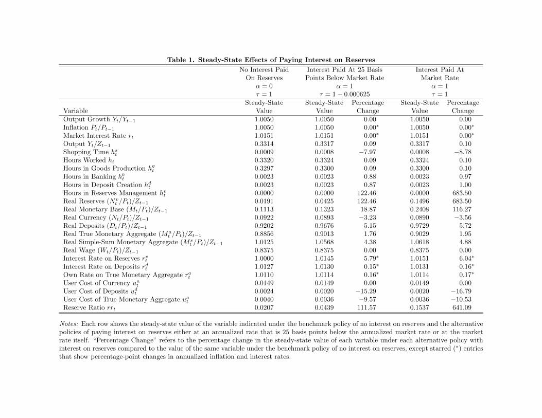
Table 1. Steady-State Effects of Paying Interest on Reserves

No Interest Paid Interest Paid At 25 Basis Interest Paid AtOn Reserves Points Below Market Rate Market Rate

α = 0 α = 1 α = 1τ = 1 τ = 1 − 0.000625 τ = 1

Steady-State Steady-State Percentage Steady-State PercentageVariable Value Value Change Value ChangeOutput Growth Yt/Yt−1 1.0050 1.0050 0.00 1.0050 0.00Inflation Pt/Pt−1 1.0050 1.0050 0.00∗ 1.0050 0.00∗

Market Interest Rate rt 1.0151 1.0151 0.00∗ 1.0151 0.00∗

Output Yt/Zt−1 0.3314 0.3317 0.09 0.3317 0.10Shopping Time hst 0.0009 0.0008 −7.97 0.0008 −8.78Hours Worked ht 0.3320 0.3324 0.09 0.3324 0.10Hours in Goods Production hgt 0.3297 0.3300 0.09 0.3300 0.10Hours in Banking hbt 0.0023 0.0023 0.88 0.0023 0.97Hours in Deposit Creation hdt 0.0023 0.0023 0.87 0.0023 1.00Hours in Reserves Management hvt 0.0000 0.0000 122.46 0.0000 683.50Real Reserves (Nv

t /Pt)/Zt−1 0.0191 0.0425 122.46 0.1496 683.50Real Monetary Base (Mt/Pt)/Zt−1 0.1113 0.1323 18.87 0.2408 116.27Real Currency (Nt/Pt)/Zt−1 0.0922 0.0893 −3.23 0.0890 −3.56Real Deposits (Dt/Pt)/Zt−1 0.9202 0.9676 5.15 0.9729 5.72Real True Monetary Aggregate (Ma

t /Pt)/Zt−1 0.8856 0.9013 1.76 0.9029 1.95Real Simple-Sum Monetary Aggregate (Ms

t /Pt)/Zt−1 1.0125 1.0568 4.38 1.0618 4.88Real Wage (Wt/Pt)/Zt−1 0.8375 0.8375 0.00 0.8375 0.00Interest Rate on Reserves rvt 1.0000 1.0145 5.79∗ 1.0151 6.04∗

Interest Rate on Deposits rdt 1.0127 1.0130 0.15∗ 1.0131 0.16∗

Own Rate on True Monetary Aggregate rat 1.0110 1.0114 0.16∗ 1.0114 0.17∗

User Cost of Currency unt 0.0149 0.0149 0.00 0.0149 0.00User Cost of Deposits udt 0.0024 0.0020 −15.29 0.0020 −16.79User Cost of True Monetary Aggregate uat 0.0040 0.0036 −9.57 0.0036 −10.53Reserve Ratio rrt 0.0207 0.0439 111.57 0.1537 641.09

Notes: Each row shows the steady-state value of the variable indicated under the benchmark policy of no interest on reserves and the alternativepolicies of paying interest on reserves either at an annualized rate that is 25 basis points below the annualized market rate or at the marketrate itself. “Percentage Change” refers to the percentage change in the steady-state value of each variable under each alternative policy withinterest on reserves compared to the value of the same variable under the benchmark policy of no interest on reserves, except starred (∗) entriesthat show percentage-point changes in annualized inflation and interest rates.

 

     

Figure  1.  Panels  (a)  and  (b)  

 

     

Figure  1.  Panels  (c)  and  (d)  

 

     

Figure  1.  Panels  (e)  and  (f)  

Figure 2. Responses of Macroeconomic Variables to Macroeconomic Shocks. Each panel shows the percentage-point response of theindicated variable to the indicated shock. Output is in log-levels; the inflation and interest rates are in annualized terms.Solid lines track the responses under the benchmark policy without interest on reserves; dashed lines track the responsesunder the alternative policy when interest is paid on reserves at a rate that is 25 basis points below the market rate.

-­‐0.05  

0  

0.05  

0.1  

0.15  

0.2  

0.25  

0   2   4   6   8   10   12   14   16  

Output  to  Preference  Shock  

0  

0.05  

0.1  

0.15  

0.2  

0.25  

0.3  

0   2   4   6   8   10   12   14   16  

Infla�on  to  Preference  Shock  

0  

0.05  

0.1  

0.15  

0.2  

0   2   4   6   8   10   12   14   16  

Market  Rate  to  Preference  Shock  

0  

0.2  

0.4  

0.6  

0.8  

1  

1.2  

0   2   4   6   8   10   12   14   16  

Output  to  Technology  Shock  

-­‐0.9  -­‐0.8  -­‐0.7  -­‐0.6  -­‐0.5  -­‐0.4  -­‐0.3  -­‐0.2  -­‐0.1  

0  

0   2   4   6   8   10   12   14   16  

Infla�on  to  Technology  Shock  

0  0.01  0.02  0.03  0.04  0.05  0.06  0.07  0.08  0.09  

0   2   4   6   8   10   12   14   16  

Market  Rate  to  Technology  Shock  

-­‐0.3  

-­‐0.25  

-­‐0.2  

-­‐0.15  

-­‐0.1  

-­‐0.05  

0  

0   2   4   6   8   10   12   14   16  

Output  to  Monetary  Policy  Shock  

-­‐0.35  

-­‐0.3  

-­‐0.25  

-­‐0.2  

-­‐0.15  

-­‐0.1  

-­‐0.05  

0  

0   2   4   6   8   10   12   14   16  

Infla�on  to  Monetary  Policy  Shock  

0  

0.05  

0.1  

0.15  

0.2  

0.25  

0.3  

0   2   4   6   8   10   12   14   16  

Market  Rate  to  Monetary  Policy  Shock  

Figure 3. Responses of Money Growth to Macroeconomic Shocks. Each panel shows the percentage-point response of the annualizedgrowth rate of the indicated monetary asset or aggregate to the indicated shock. Solid lines track the responses under thebenchmark policy without interest on reserves; dashed lines track the responses under the alternative policy when interest ispaid on reserves at a rate that is 25 basis points below the market rate.

-­‐2  

-­‐1.5  

-­‐1  

-­‐0.5  

0  

0.5  

1  

1.5  

2  

0   2   4   6   8   10   12   14   16  

Reserves  to  Preference  Shock  

-­‐5  

-­‐4  

-­‐3  

-­‐2  

-­‐1  

0  

1  

2  

0   2   4   6   8   10   12   14   16  

Monetary  Base  to  Preference  Shock  

-­‐5  

-­‐4  

-­‐3  

-­‐2  

-­‐1  

0  

1  

2  

0   2   4   6   8   10   12   14   16  

Currency  to  Preference  Shock  

-­‐0.5  

0  

0.5  

1  

1.5  

2  

0   2   4   6   8   10   12   14   16  

Deposits  to  Preference  Shock  

-­‐1.5  

-­‐1  

-­‐0.5  

0  

0.5  

1  

1.5  

0   2   4   6   8   10   12   14   16  

True  Aggregate  to  Preference  Shock  

-­‐0.2  

0  

0.2  

0.4  

0.6  

0.8  

1  

1.2  

0   2   4   6   8   10   12   14   16  

Simple  Sum  Aggregate  to  Preference  Shock  

-­‐0.8  -­‐0.6  -­‐0.4  -­‐0.2  

0  0.2  0.4  0.6  0.8  1  

1.2  

0   2   4   6   8   10   12   14   16  

Reserves  to  Technology  Shock  

-­‐2  

-­‐1.5  

-­‐1  

-­‐0.5  

0  

0.5  

1  

0   2   4   6   8   10   12   14   16  

Monetary  Base  to  Technology  Shock  

-­‐2  

-­‐1.5  

-­‐1  

-­‐0.5  

0  

0.5  

1  

0   2   4   6   8   10   12   14   16  

Currency  to  Technology  Shock  

-­‐0.5  

0  

0.5  

1  

1.5  

2  

0   2   4   6   8   10   12   14   16  

Deposits  to  Technology  Shock  

-­‐0.6  -­‐0.4  -­‐0.2  

0  0.2  0.4  0.6  0.8  1  

1.2  

0   2   4   6   8   10   12   14   16  

True  Aggregate  to  Technology  Shock  

-­‐0.4  -­‐0.2  

0  0.2  0.4  0.6  0.8  1  

1.2  1.4  1.6  

0   2   4   6   8   10   12   14   16  

Simple  Sum  Aggregate  to  Technology  Shock  

-­‐4  

-­‐3  

-­‐2  

-­‐1  

0  

1  

2  

3  

0   2   4   6   8   10   12   14   16  

Reserves  to  Monetary  Policy  Shock  

-­‐8  

-­‐6  

-­‐4  

-­‐2  

0  

2  

4  

6  

0   2   4   6   8   10   12   14   16  

Monetary  Base  to  Monetary  Policy  Shock  

-­‐10  -­‐8  -­‐6  -­‐4  -­‐2  0  2  4  6  8  

0   2   4   6   8   10   12   14   16  

Currency  to  Monetary  Policy  Shock  

-­‐2.5  

-­‐2  

-­‐1.5  

-­‐1  

-­‐0.5  

0  

0.5  

1  

1.5  

0   2   4   6   8   10   12   14   16  

Deposits  to  Monetary  Policy  Shock  

-­‐3  -­‐2.5  -­‐2  

-­‐1.5  -­‐1  

-­‐0.5  0  

0.5  1  

1.5  

0   2   4   6   8   10   12   14   16  

True  Aggregate  to  Monetary  Policy  Shock  

-­‐1.5  

-­‐1  

-­‐0.5  

0  

0.5  

1  

0   2   4   6   8   10   12   14   16  

Simple  Sum  Aggregate  to  Monetary  Policy  Shock  

Figure 4. Responses of Financial Variables to Macroeconomic Shocks. Each panel shows the percentage-point response of the indicatedvariable to the indicated shock. The reserves rate is annualized; the other variables are not. Solid lines track responses under thebenchmark policy without interest on reserves; dashed lines track the responses under the alternative policy when interest ispaid on reserves at a rate that is 25 basis points below the market rate.

0  

0.05  

0.1  

0.15  

0.2  

0   2   4   6   8   10   12   14   16  

Reserves  Rate  to  Preference  Shock  

-­‐0.1  

0  

0.1  

0.2  

0.3  

0.4  

0.5  

0   2   4   6   8   10   12   14   16  

UC  of  Deposits  to  Preference  Shock  

0  

0.2  

0.4  

0.6  

0.8  

1  

1.2  

1.4  

1.6  

0   2   4   6   8   10   12   14   16  

UC  of  True  Aggregate  to  Preference  Shock  

0  0.01  0.02  0.03  0.04  0.05  0.06  0.07  0.08  0.09  

0   2   4   6   8   10   12   14   16  

Reserves  Rate  to  Technology  Shock  

-­‐0.7  

-­‐0.6  

-­‐0.5  

-­‐0.4  

-­‐0.3  

-­‐0.2  

-­‐0.1  

0  

0   2   4   6   8   10   12   14   16  

UC  of  Deposits  to  Technology  Shock  

-­‐0.4  -­‐0.3  -­‐0.2  -­‐0.1  

0  0.1  0.2  0.3  0.4  0.5  

0   2   4   6   8   10   12   14   16  

UC  of  True  Aggregate  to  Technology  Shock  

0  

0.05  

0.1  

0.15  

0.2  

0.25  

0.3  

0   2   4   6   8   10   12   14   16  

Reserves  Rate  to  Monetary  Policy  Shock  

-­‐0.4  

-­‐0.3  

-­‐0.2  

-­‐0.1  

0  

0.1  

0.2  

0.3  

0.4  

0   2   4   6   8   10   12   14   16  

UC  of  Deposits  to  Monetary  Policy  Shock  

0  

0.5  

1  

1.5  

2  

0   2   4   6   8   10   12   14   16  

UC  of  True  Aggregate  to  Monetary  Policy  Shock  

0  

0.5  

1  

1.5  

2  

2.5  

3  

3.5  

0   2   4   6   8   10   12   14   16  

UC  of  Currency  to  Preference  Shock  

0  

0.2  

0.4  

0.6  

0.8  

1  

1.2  

1.4  

0   2   4   6   8   10   12   14   16  

UC  of  Currency  to  Technology  Shock  

0  0.5  1  

1.5  2  

2.5  3  

3.5  4  

4.5  

0   2   4   6   8   10   12   14   16  

UC  of  Currency  to  Monetary  Policy  Shock  

Figure 5. Responses of Macroeconomic Variables to Financial Shocks. Each panel shows the percentage-point response of the indicatedvariable to the indicated shock. Output is in log-levels; the inflation and interest rates are in annualized terms. Solid lines trackthe responses under the benchmark policy without interest on reserves; dashed lines track the responses under the alternativepolicy when interest is paid on reserves at a rate that is 25 basis points below the market rate.

-­‐0.01  

-­‐0.008  

-­‐0.006  

-­‐0.004  

-­‐0.002  

0  

0   2   4   6   8   10   12   14   16  

Output  to  Money  Demand  Shock  

-­‐0.01  

-­‐0.005  

0  

0.005  

0.01  

0   2   4   6   8   10   12   14   16  

Infla�on  to  Money  Demand  Shock  

-­‐0.01  

-­‐0.008  

-­‐0.006  

-­‐0.004  

-­‐0.002  

0  

0   2   4   6   8   10   12   14   16  

Market  Rate  to  Money  Demand  Shock  

-­‐1.2  

-­‐1  

-­‐0.8  

-­‐0.6  

-­‐0.4  

-­‐0.2  

0  

0   2   4   6   8   10   12   14   16  

Output  to  Bank  Produc�vity  Shock  

-­‐0.08  

-­‐0.06  

-­‐0.04  

-­‐0.02  

0  

0.02  

0.04  

0.06  

0   2   4   6   8   10   12   14   16  

Infla�on  to  Bank  Produc�vity  Shock  

-­‐0.7  

-­‐0.6  

-­‐0.5  

-­‐0.4  

-­‐0.3  

-­‐0.2  

-­‐0.1  

0  

0.1  

0   2   4   6   8   10   12   14   16  

Market  Rate  to  Bank  Produc�vity  Shock  

0  

0.002  

0.004  

0.006  

0.008  

0.01  

0   2   4   6   8   10   12   14   16  

Output  to  Reserves  Rate  Shock  

-­‐0.01  

-­‐0.005  

0  

0.005  

0.01  

0   2   4   6   8   10   12   14   16  

Infla�on  to  Reserves  Rate  Shock  

0  

0.002  

0.004  

0.006  

0.008  

0.01  

0   2   4   6   8   10   12   14   16  

Market  Rate  to  Reserves  Rate  Shock  

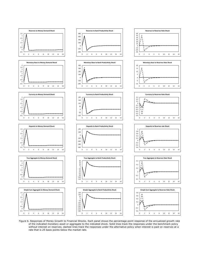
Figure 6. Responses of Money Growth to Financial Shocks. Each panel shows the percentage-point response of the annualized growth rateof the indicated monetary asset or aggregate to the indicated shock. Solid lines track the responses under the benchmark policywithout interest on reserves; dashed lines track the responses under the alternative policy when interest is paid on reserves at arate that is 25 basis points below the market rate.

-­‐0.5  

0  

0.5  

1  

1.5  

2  

2.5  

3  

3.5  

0   2   4   6   8   10   12   14   16  

Reserves  to  Money  Demand  Shock  

-­‐0.5  0  

0.5  1  

1.5  2  

2.5  3  

3.5  4  

0   2   4   6   8   10   12   14   16  

Monetary  Base  to  Money  Demand  Shock  

-­‐0.5  0  

0.5  1  

1.5  2  

2.5  3  

3.5  4  

0   2   4   6   8   10   12   14   16  

Currency  to  Money  Demand  Shock  

-­‐0.5  

0  

0.5  

1  

1.5  

2  

2.5  

3  

3.5  

0   2   4   6   8   10   12   14   16  

Deposits  to  Money  Demand  Shock  

-­‐0.5  

0  

0.5  

1  

1.5  

2  

2.5  

3  

3.5  

0   2   4   6   8   10   12   14   16  

True  Aggregate  to  Money  Demand  Shock  

-­‐0.5  

0  

0.5  

1  

1.5  

2  

2.5  

3  

3.5  

0   2   4   6   8   10   12   14   16  

Simple  Sum  Aggregate  to  Money  Demand  Shock  

-­‐400  

-­‐200  

0  

200  

400  

600  

800  

0   2   4   6   8   10   12   14   16  

Reserves  to  Bank  Produc�vity  Shock  

-­‐200  

-­‐100  

0  

100  

200  

300  

400  

0   2   4   6   8   10   12   14   16  

Monetary  Base  to  Bank  Produc�vity  Shock  

-­‐100  

-­‐50  

0  

50  

100  

150  

200  

0   2   4   6   8   10   12   14   16  

Currency  to  Bank  Produc�vity  Shock  

-­‐400  

-­‐300  

-­‐200  

-­‐100  

0  

100  

200  

0   2   4   6   8   10   12   14   16  

Deposits  to  Bank  Produc�vity  Shock  

-­‐120  -­‐100  -­‐80  -­‐60  -­‐40  -­‐20  0  

20  40  60  

0   2   4   6   8   10   12   14   16  

True  Aggregate  to  Bank  Produc�vity  Shock  

-­‐300  -­‐250  -­‐200  -­‐150  -­‐100  -­‐50  0  

50  100  150  

0   2   4   6   8   10   12   14   16  

Simple  Aggregate  to  Bank  Produc�vity  Shock  

-­‐30  -­‐20  -­‐10  0  

10  20  30  40  50  60  

0   2   4   6   8   10   12   14   16  

Reserves  to  Reserves  Rate  Shock  

-­‐10  

-­‐5  

0  

5  

10  

15  

20  

0   2   4   6   8   10   12   14   16  

Monetary  Base  to  Reserves  Rate  Shock  

-­‐0.6  -­‐0.5  -­‐0.4  -­‐0.3  -­‐0.2  -­‐0.1  

0  0.1  0.2  0.3  

0   2   4   6   8   10   12   14   16  

Currency  to  Reserves  Rate  Shock  

-­‐0.6  

-­‐0.4  

-­‐0.2  

0  

0.2  

0.4  

0.6  

0.8  

1  

0   2   4   6   8   10   12   14   16  

Deposits  to  Reserves  rate  Shock  

-­‐0.2  

-­‐0.1  

0  

0.1  

0.2  

0.3  

0   2   4   6   8   10   12   14   16  

True  Aggregate  to  Reserves  Rate  Shock  

-­‐0.4  

-­‐0.2  

0  

0.2  

0.4  

0.6  

0.8  

0   2   4   6   8   10   12   14   16  

Simple  Sum  Aggregate  to  Reserves  Rate  Shock  

Figure 7. Responses of Financial Variables to Financial Shocks. Each panel shows the percentage-point response of the indicated variableto the indicated shock. The reserves rate is annualized; the other variables are not. Solid lines track the responses under thebenchmark policy without interest on reserves; dashed lines track the responses under the alternative policy when interest ispaid on reserves at a rate that is 25 basis points below the market rate.

-­‐0.01  

-­‐0.008  

-­‐0.006  

-­‐0.004  

-­‐0.002  

0  

0   2   4   6   8   10   12   14   16  

Reserves  Rate  to  Money  Demand  Shock  

-­‐0.01  

-­‐0.005  

0  

0.005  

0.01  

0   2   4   6   8   10   12   14   16  

UC  of  Deposits  to  Money  Demand  Shock  

-­‐0.016  -­‐0.014  -­‐0.012  -­‐0.01  -­‐0.008  -­‐0.006  -­‐0.004  -­‐0.002  

0  0.002  0.004  

0   2   4   6   8   10   12   14   16  

UC  of  True  Aggregate  to  Money  Demand  Shock  

-­‐0.6  

-­‐0.5  

-­‐0.4  

-­‐0.3  

-­‐0.2  

-­‐0.1  

0  

0.1  

0   2   4   6   8   10   12   14   16  

Reserves  Rate  to  Bank  Produc�vity  Shock  

0  

50  

100  

150  

200  

250  

0   2   4   6   8   10   12   14   16  

UC  of  Deposits  to  Bank  Produc�vity  Shock  

0  

20  

40  

60  

80  

100  

120  

140  

160  

0   2   4   6   8   10   12   14   16  

UC  of  True  Aggregate  to  Bank  Produc�vity  Shock  

0  

0.02  

0.04  

0.06  

0.08  

0.1  

0.12  

0.14  

0   2   4   6   8   10   12   14   16  

Reserves  Rate  to  Reserves  Rate  Shock  

-­‐0.8  

-­‐0.7  

-­‐0.6  

-­‐0.5  

-­‐0.4  

-­‐0.3  

-­‐0.2  

-­‐0.1  

0  

0   2   4   6   8   10   12   14   16  

UC  of  Deposits  to  Reserves  Rate  Shock  

-­‐0.45  -­‐0.4  -­‐0.35  -­‐0.3  -­‐0.25  -­‐0.2  -­‐0.15  -­‐0.1  -­‐0.05  

0  

0   2   4   6   8   10   12   14   16  

UC  of  True  Aggregate  to  Reserves  Rate  Shock  

-­‐0.035  

-­‐0.03  

-­‐0.025  

-­‐0.02  

-­‐0.015  

-­‐0.01  

-­‐0.005  

0  

0   2   4   6   8   10   12   14   16  

UC  of  Currency  to  Money  Demand  Shock  

-­‐12  

-­‐10  

-­‐8  

-­‐6  

-­‐4  

-­‐2  

0  

2  

0   2   4   6   8   10   12   14   16  

UC  of  Currency  to  Bank  Produc�vity  Shock  

0  

0.005  

0.01  

0.015  

0.02  

0.025  

0.03  

0   2   4   6   8   10   12   14   16  

UC  of  Currency  to  Reserves  Rate  Shock  

Figure 8. Responses of Macroeconomic and Money Growth Variables to Macroeconomic and Financial Shocks. Derived using the alternative calibration described in the text. Each panelshows the percentage-point response of the indicated variable to the indicated shock. Output is in log-levels; the inflation, interest, and money growth rates are in annualizedterms. Solid lines track the responses under the benchmark policy without interest on reserves; dashed lines track the responses under the alternative policy when interest ispaid on reserves at a rate that is 25 basis points below the market rate.

-­‐0.15  

-­‐0.1  

-­‐0.05  

0  

0.05  

0.1  

0.15  

0.2  

0   2   4   6   8   10   12   14   16  

Output  to  Preference  Shock  

0  

0.05  

0.1  

0.15  

0.2  

0.25  

0.3  

0.35  

0.4  

0   2   4   6   8   10   12   14   16  

Infla�on  to  Preference  Shock  

0  0.05  0.1  

0.15  0.2  

0.25  0.3  

0.35  0.4  

0.45  

0   2   4   6   8   10   12   14   16  

Market  Rate  to  Preference  Shock  

-­‐4  

-­‐3  

-­‐2  

-­‐1  

0  

1  

2  

3  

4  

0   2   4   6   8   10   12   14   16  

Reserves  to  Preference  Shock  

-­‐3.5  -­‐3  

-­‐2.5  -­‐2  

-­‐1.5  -­‐1  

-­‐0.5  0  

0.5  1  

1.5  

0   2   4   6   8   10   12   14   16  

True  Aggregate  to  Preference  Shock  

0  

0.2  

0.4  

0.6  

0.8  

1  

1.2  

0   2   4   6   8   10   12   14   16  

Output  to  Technology  Shock  

0  

0.2  

0.4  

0.6  

0.8  

1  

0   2   4   6   8   10   12   14   16  

Infla�on  to  Technology  Shock  

0  

0.2  

0.4  

0.6  

0.8  

1  

0   2   4   6   8   10   12   14   16  

Market  Rate  to  Technology  Shock  

0  0.5  1  

1.5  2  

2.5  3  

3.5  4  

4.5  

0   2   4   6   8   10   12   14   16  

Reserves  to  Technology  Shock  

0  0.5  1  

1.5  2  

2.5  3  

3.5  4  

4.5  

0   2   4   6   8   10   12   14   16  

True  Aggregate  to  Technology  Shock  

-­‐0.16  

-­‐0.14  

-­‐0.12  

-­‐0.1  

-­‐0.08  

-­‐0.06  

-­‐0.04  

-­‐0.02  

0  

0   2   4   6   8   10   12   14   16  

Output  to  Monetary  Policy  Shock  

-­‐0.035  

-­‐0.03  

-­‐0.025  

-­‐0.02  

-­‐0.015  

-­‐0.01  

-­‐0.005  

0  

0   2   4   6   8   10   12   14   16  

Infla�on  to  Monetary  Policy  Shock  

0  

0.05  

0.1  

0.15  

0.2  

0.25  

0.3  

0   2   4   6   8   10   12   14   16  

Market  Rate  to  Monetary  Policy  Shock  

-­‐4  

-­‐3  

-­‐2  

-­‐1  

0  

1  

2  

3  

4  

0   2   4   6   8   10   12   14   16  

Reserves  to  Monetary  Policy  Shock  

-­‐4  

-­‐3  

-­‐2  

-­‐1  

0  

1  

2  

0   2   4   6   8   10   12   14   16  

True  Aggregate  to  Monetary  Policy  Shock  

0  

0.01  

0.02  

0.03  

0.04  

0.05  

0.06  

0.07  

0   2   4   6   8   10   12   14   16  

Output  to  Reserves  Rate  Shock  

0  

0.2  

0.4  

0.6  

0.8  

1  

0   2   4   6   8   10   12   14   16  

Infla�on  to  Reserves  Rate  Shock  

0  

0.2  

0.4  

0.6  

0.8  

1  

0   2   4   6   8   10   12   14   16  

Market  Rate  to  Reserves  Rate  Shock  

-­‐40  -­‐30  -­‐20  -­‐10  0  

10  20  30  40  50  60  

0   2   4   6   8   10   12   14   16  

Reserves  to  Reserves  Rate  Shock  

-­‐1.5  -­‐1  

-­‐0.5  0  

0.5  1  

1.5  2  

2.5  3  

0   2   4   6   8   10   12   14   16  

True  Aggregate  to  Reserves  Rate  Shock