the lexis diagram, a misnomer - demographic research · demographic research - volume 4, article 3 ...

Demographic Research a free, expedited, online journal of peer-reviewed research and commentary in the population sciences published by the Max Planck Institute for Demographic Research Doberaner Strasse 114 · D-18057 Rostock · GERMANY www.demographic-research.org

DEMOGRAPHIC RESEARCH VOLUME 4, ARTICLE 3, PAGES 97-124 PUBLISHED 9 MARCH 2001 www.demographic-research.org/Volumes/Vol4/3/ DOI: 10.4054/DemRes.2001.4.3

The Lexis diagram, a misnomer

Christophe Vandeschrick

© 2001 Max-Planck-Gesellschaft.

Table of Contents

1. Introduction 98

2. The construction of the diagrams 982.1 Lexis 982.2 From three to two axes or the emergence of three

equivalent solutions103

2.2.1 The “moment of birth and age” diagram 1042.2.2 The “time and age” diagram 1052.2.3 The “time and moment of birth” diagram 107

3. But who then invented the Lexis diagram? 1083.1 The controversy 1083.2 The development of the three diagrams 1093.2.1 The diagram “time and moment of birth” 1103.2.2 The diagram “moment of birth and age" 1103.2.3 The diagram “time and age” or Brasche, the great

forgotten111

3.2.4 The diagram race: prize giving 112

4. Conclusions 113

Notes 115

References 118

A. Appendix A. Original Quotations 121

Demographic Research - Volume 4, Article 3

http://www.demographic-research.org 97

The Lexis diagram, a misnomer 1

Christophe Vandeschrick 2

Abstract

Around 1870, demographers felt the need for a simple chart to present population

dynamics. This chart is known as the “Lexis diagram”, but it is a misnomer. To be useful,

this chart must allow for the systematic location on one plane of the three classical

demographic co-ordinates, namely: the date, the age and the moment of birth. There are

three solutions for this problem. In 1869, Zeuner worked out a first solution. In 1870,

Brasche proposed a second one with networks of parallels; it is the version most currently

used now. In 1874, Becker proposed the third one. In 1875, certainly after Verwey, Lexis

took back Zeuner’s diagram and just added networks of parallels. In spite of all this, the

name “Lexis diagram” has imposed itself in a seemingly invincible way.

1 A previous version of this work was presented in August 2000 at the workshop "Lexis in Context" held

at the Max Planck Institute for Demographic Research in Rostock, Germany.2 Institut de Démographie, Université catholique de Louvain; 1, place Montesquieu, Bte 17;

B – 1348 – Louvain-la-Neuve; Belgique. E-mail: [email protected]


98 http://www.demographic-research.org

1. Introduction

Around 1870, demographers, particularly in Germany, felt the need for a simple chart topresent population dynamics, especially in view of establishing life table formulas.What principal quality should this graph present? To be fully useful, it must allow forthe systematic location on one plane of the three co-ordinates used to classify deaths andsurvivors, namely: the date, the age and the moment of birth. The diagram obtained issomewhat peculiar. On the one hand it allows for a construction according to two axesbut also for three co-ordinates, while on the other, the population figures can be locatedin keeping with certain criteria expressed in terms of the three co-ordinates rather thanthe evolution of one variable in relation to another.

Among the authors who contributed to the making of this tool, it was Lexis whogave it its name. Our communication none the less calls into question theappropriateness of the name “Lexis diagram”. In fact, the question of its paternity wasquite controversial in the nineteenth century.

The first part of our paper explains the various solutions proposed to represent thethree demographic co-ordinates on a diagram with two axes. The second part aims atreconstructing their history so as to determine who their true father really is. It should benoted that this search is not definitively completed. Certain documents should still beconsulted or could even be discovered. However, documentation currently at ourdisposal enables us to conclude in a relatively sure way. The German texts of thebibliography were (partially) translated into French (Note 1).

2. The construction of the diagrams

According to the authors considered in this paper, the development of the diagramrepresenting the three demographic co-ordinates on one plane, is explained in differentways. It seems interesting to start by exposing the steps followed by Lexis himself. Wethen propose a different explanation, to some extent more logical, to show the de factoequivalence of the various forms taken by the diagram.

2.1 Lexis

Lexis aimed to locate deaths (Note 2) on a simple graph according to the threefollowing demographic co-ordinates:- the moment of death;- the age of the deceased at the moment of death;- the moment of birth of the deceased.



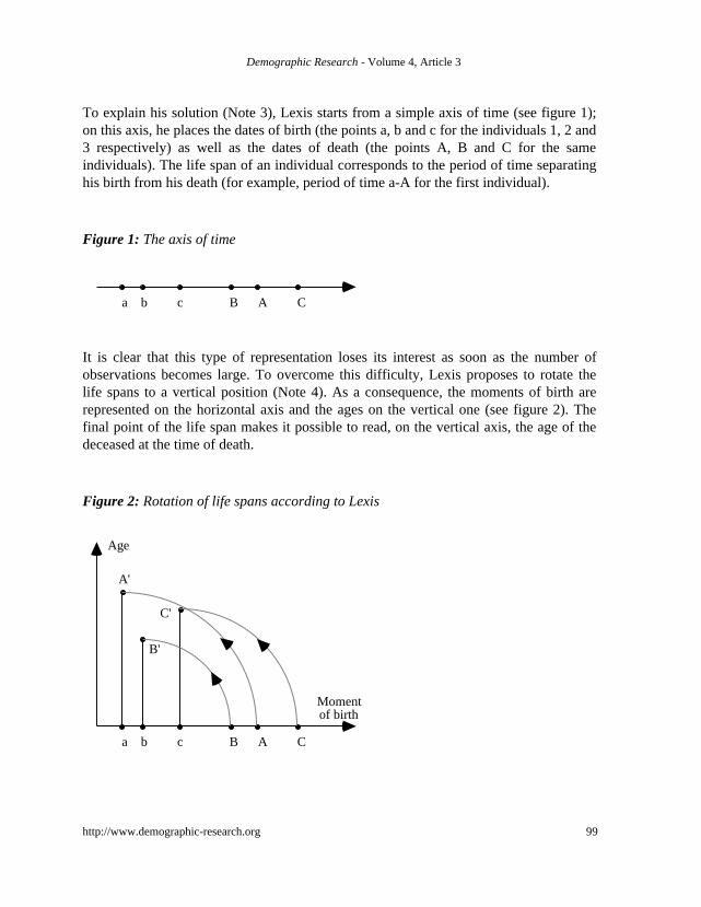
To explain his solution (Note 3), Lexis starts from a simple axis of time (see figure 1);on this axis, he places the dates of birth (the points a, b and c for the individuals 1, 2 and3 respectively) as well as the dates of death (the points A, B and C for the sameindividuals). The life span of an individual corresponds to the period of time separatinghis birth from his death (for example, period of time a-A for the first individual).

Figure 1: The axis of time

a b c B A C

It is clear that this type of representation loses its interest as soon as the number ofobservations becomes large. To overcome this difficulty, Lexis proposes to rotate thelife spans to a vertical position (Note 4). As a consequence, the moments of birth arerepresented on the horizontal axis and the ages on the vertical one (see figure 2). Thefinal point of the life span makes it possible to read, on the vertical axis, the age of thedeceased at the time of death.

Figure 2: Rotation of life spans according to Lexis

a b c B A C

Age

Moment of birth

A'

B'

C'



Using such a construction, all the events occurring at a precise moment in time can belocated on a decreasing oblique (see figure 3). This isochronal line is called“isochrone”; its intersection with the axis of the moments of birth, determines themoment that it is represented on the diagram: in the case of figure 3, the obliquecorresponds to the date 1/1/87. At this date, an individual born on the 1/1/84 was 3years old (see dot “p”); another born on 1/1/86 was 1 year of age (see dot “q”).

Figure 3: An isochrone

Age

1983 1984 1985 19860

1

2

3

4

5

Moment of birth

1987

p

q

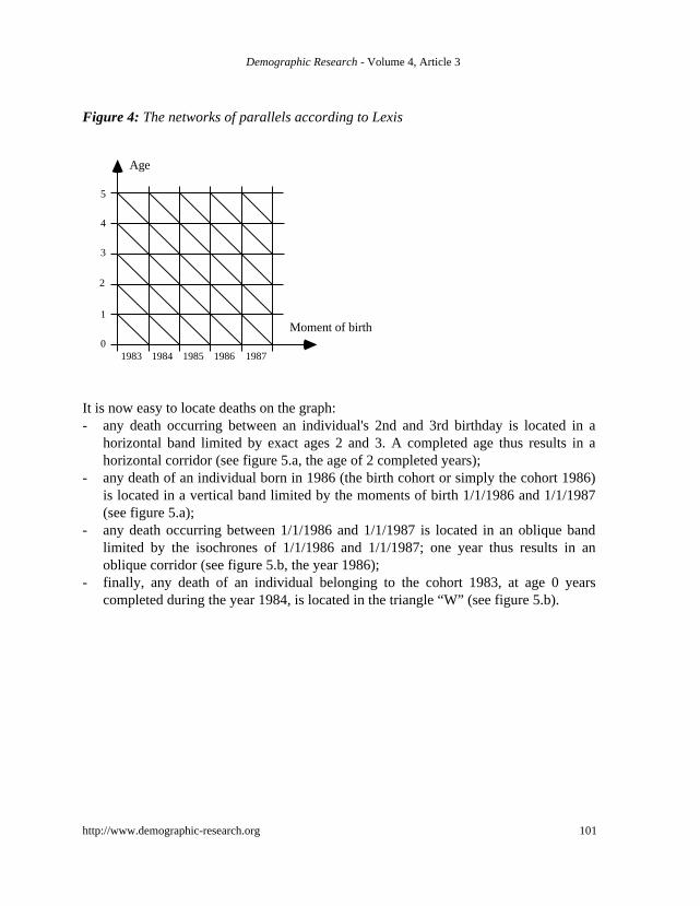
To be used easily, networks of parallel lines corresponding to particular co-ordinatescomplete the graph (see figure 4):- the horizontal ones for the exact ages;- the vertical ones for the moments of birth (corresponding to the beginning or end of

the year);- the decreasing oblique lines for the dates (corresponding to the beginning or end of

the year.



Figure 4: The networks of parallels according to Lexis

Age

1983 1984 1985 19860

1

2

3

4

5

Moment of birth

1987

It is now easy to locate deaths on the graph:- any death occurring between an individual's 2nd and 3rd birthday is located in a

horizontal band limited by exact ages 2 and 3. A completed age thus results in ahorizontal corridor (see figure 5.a, the age of 2 completed years);

- any death of an individual born in 1986 (the birth cohort or simply the cohort 1986)is located in a vertical band limited by the moments of birth 1/1/1986 and 1/1/1987(see figure 5.a);

- any death occurring between 1/1/1986 and 1/1/1987 is located in an oblique bandlimited by the isochrones of 1/1/1986 and 1/1/1987; one year thus results in anoblique corridor (see figure 5.b, the year 1986);

- finally, any death of an individual belonging to the cohort 1983, at age 0 yearscompleted during the year 1984, is located in the triangle “W” (see figure 5.b).



Figure 5: The localisation of the co-ordinates

Age

1983 1984 1985 19860

1

2

3

4

5

Moment of birth

1987

Age

1983 1984 1985 19860

1

2

3

4

5

1987

5.a 5.b

2 completed years

Cohort '86

Year '86

W

This construction is entirely satisfactory since it allows for the systematic location of thethree demographic co-ordinates. The diagram comprises only two axes, reserved for themoment of birth, on the horizontal axis, and, for age, on the vertical one. These two co-ordinates are classically represented by lines perpendicular to their axis. The third co-ordinate - time or moment of death – parasites the horizontal axis (Note 5) and isfigured by an oblique.

Thus the horizontal axis supports two co-ordinates: the moment of birth and thetime. The moment of birth can be considered as the “host” co-ordinate, in that itwelcomes on its axis another co-ordinate, time. This latter can thus be taken as aparasitical co-ordinate, for it occupies a spot on an axis which is not its own (Note 6).

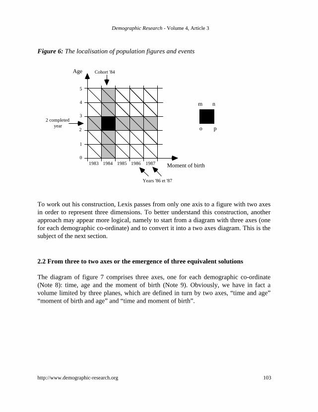
On this graph, the population figures for deceased and survivors can be readilylocated according to the three demographic co-ordinates (Note 7). It thus becomespossible to visualise the elements necessary to calculate the probability of dying and toconnect corresponding elements correctly: in particular deaths must be divided by thepopulation figure subject to the risk of dying. For example (see figure 6), to calculatethe risk of dying for individuals born in 1984, between age 2 and 3, we should dividethe deaths located in square “mnop” (i.e. the intersection between the horizontal band ofcompleted age 2 and the vertical band of the cohort 1984) by the survivors on line “op”(i.e. the survivors of the cohort 1984 up to 2 years exactly). These deaths occurredduring 2 years: 1986 and 1987. The diagram thus achieves its goal: it is indeed aprecious tool to determine the way to calculate an index correctly.



Figure 6: The localisation of population figures and events

Age

1983 1984 1985 19860

1

2

3

4

5

Moment of birth1987

o p

m n

Cohort '84

2 completed year

Years '86 et '87

To work out his construction, Lexis passes from only one axis to a figure with two axesin order to represent three dimensions. To better understand this construction, anotherapproach may appear more logical, namely to start from a diagram with three axes (onefor each demographic co-ordinate) and to convert it into a two axes diagram. This is thesubject of the next section.

2.2 From three to two axes or the emergence of three equivalent solutions

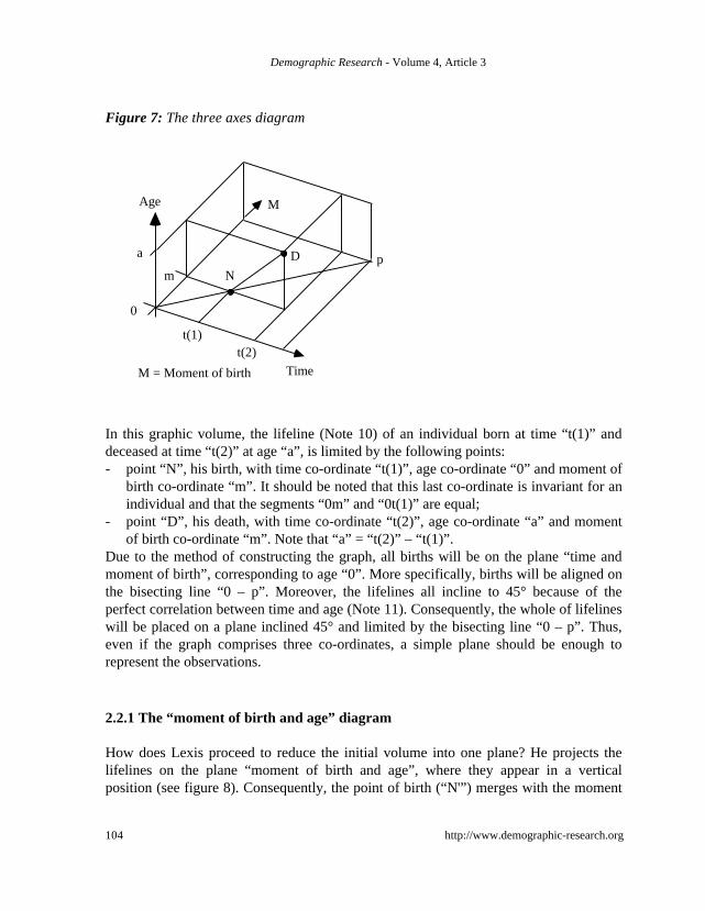
The diagram of figure 7 comprises three axes, one for each demographic co-ordinate(Note 8): time, age and the moment of birth (Note 9). Obviously, we have in fact avolume limited by three planes, which are defined in turn by two axes, “time and age”“moment of birth and age” and “time and moment of birth”.



Figure 7: The three axes diagram

Age

TimeM = Moment of birth

M

t(1)t(2)

0

a

m ND p

In this graphic volume, the lifeline (Note 10) of an individual born at time “t(1)” anddeceased at time “t(2)” at age “a”, is limited by the following points:- point “N”, his birth, with time co-ordinate “t(1)”, age co-ordinate “0” and moment of

birth co-ordinate “m”. It should be noted that this last co-ordinate is invariant for anindividual and that the segments “0m” and “0t(1)” are equal;

- point “D”, his death, with time co-ordinate “t(2)”, age co-ordinate “a” and momentof birth co-ordinate “m”. Note that “a” = “t(2)” – “t(1)”.

Due to the method of constructing the graph, all births will be on the plane “time andmoment of birth”, corresponding to age “0”. More specifically, births will be aligned onthe bisecting line “0 – p”. Moreover, the lifelines all incline to 45° because of theperfect correlation between time and age (Note 11). Consequently, the whole of lifelineswill be placed on a plane inclined 45° and limited by the bisecting line “0 – p”. Thus,even if the graph comprises three co-ordinates, a simple plane should be enough torepresent the observations.

2.2.1 The “moment of birth and age” diagram

How does Lexis proceed to reduce the initial volume into one plane? He projects thelifelines on the plane “moment of birth and age”, where they appear in a verticalposition (see figure 8). Consequently, the point of birth (“N'”) merges with the moment



of birth co-ordinate (“m”). The point of death (“D”) moves to the vertical axis of thispoint “m” at the height of age “a”. Here, the “host” co-ordinate is the moment of birthand the “parasite” is the time co-ordinate. As already indicated, the graph will becompleted by networks of parallels (see figure 4). On this figure, an oblique line mustbe interpreted in the following way: the evolution of age according to the moment ofbirth at a given date (see figure 3).

Figure 8: The projection on the “moment of birth and age” plane

Age


M

t(1)t(2)

0

a

m ND pN'

D' Age

Moment of birth and time

0

a

N'

D'

m

To pass from a volume to a plane, it is also possible to project on either one of the twoother planes, the “time and age” plane or the “time and moment of birth” one.

2.2.2 The “time and age” diagram

In the case of a projection on the “time and age” plane (see figure 9), the beginning of alifeline falls on the time axis at the date corresponding to birth (“N'” and “t(1)” falltogether) while the moment of death is located at the vertical position of the date ofoccurrence and at the horizontal position of the age of occurrence, i.e. point “D'”. Allthe lifelines appear in an oblique form on the plane of projection with an inclination of45°. The horizontal axis supports both the “time” and the “moment of birth” co-ordinates, the second being regarded as the “parasite” and the first one as the “host”.



Figure 9: The projection on the plane “time and age”

Age


M

t(1)t(2)

0

a

mN

D p

N'

D'

t(1) t(2)

aD'

N'

Age

Time and moment of birth

Here also the diagram will be completed by networks of parallels (see figure 10.a). Inthis graph, an oblique line is interpreted in the following way: the evolution of ageaccording to time for any one moment of birth or a given individual.

Figure 10: The networks of parallels

1983 1984 1985 1986 1987 Time and

1983

1984

1985

1986

1987

Moment of birth

1983 1984 1985 1986 19870

1

2

3

4

5

Time and moment of

birth

Age

10. b10.a

age0 1 2 3 4 5



2.2.3 The “time and moment of birth” diagram

In the case of a projection on the “time and moment of birth” plane (see figure 11), “N”and “N'” merge and “D'” is projected at the height of the moment of birth (“m”) and ofthe date of death (“t(2)”). Here the “host” co-ordinate is time, and the “parasite” is age.To be rigorously complete, the figure should thus comprise two scales under thehorizontal axis: one for time and one for age (see figure 10.b). In the first twoprojections this is not the case, since the “host” and “parasite” co-ordinates correspondon the same scale!

Figure 11: The projection on the “time and moment of birth” plane

Age


M

t(1)t(2)

0

a

mD p

D'

N et N'

Moment of birth

Time and age

0

m

t(1) t(2)

D'N et N'

Again, the diagram will be completed by networks of parallels (see figure 10.b). Anoblique is interpreted as the evolution of the moment of birth according to time for agiven age.

The three solutions (Note 12), the projections of the initial volume on each of thethree plans, are interchangeable: they all allow for the systematic location of the threedemographic co-ordinates. There is thus in fact no reason to prefer one solution over theother. However, one can consider that a projection on the “time and age” planerepresents a more “natural” solution (Note 13). The interpretation of the oblique lines asthe evolution of age according to time for an individual is less complicated than the 2other interpretations, even if, on the mathematical level, all three formulations areequivalent.



3. But who then invented the Lexis diagram?

The previous point showed that the diagram proposed by Lexis is, in fact, only one ofthe three solutions to get from three to two axes. In addition, the version most currentlyused is actually not the Lexis’ one. The form changed, the name remained. The questionof paternity then can be reformulated by two more precise sub-questions:- who was the first to suggest a satisfactory solution?- who was the first to suggest each of the three versions of the diagram?These two questions will be tackled after a quick summary of the controversy up to thebeginning of the twentieth century which took place between several researchers.

3.1 The controversy

Since 1880 (but perhaps already before) and at least until 1903, the question of thepaternity of the diagram was prone to polemics, mainly between Lexis and Zeuner. In atext of 1880, Lexis writes the following about two diagrams proposed by Becker andVerwey (Note 14):

“According to custom, the book (Note 15) is dated from 1875, even if it waspublished already in 1874. The foreword was written just before thepublication and is dated from 1874. The impression of this book was alreadybegun during the summer when Becker published his book. My work iscompletely independent of Becker’s. Soon after, Verwey published a thesis inDutch about the same subject and the application of the same principle, buthis work is independent of mine. The article of Verwey was published inEnglish in the Journal of the Statistical Society, London, in December 1875.”

Later, Zeuner will dispute the paternity assumed by Lexis in a publication of 1886 (Note16). On page 8, one can read the following:

“Lexis uses the same figure in his book "Einleitung in die Theorie derBevölkerungsstatistik" Strassburg 1875. This figure presents perpendicularaxes. So, Lexis accepts the plan of my stereometric figure. Note by the waythat Lexis does not refer to my work.” (Note 17)

Then on page 11:“Generally speaking, the figures 2 and 3 represent exactly the basic plane ofmy stereometric demonstration dated from 1869. Lexis claimed for himselfthis demonstration in 1875. All the difference between the two demonstrationsis explained as followed: Lexis uses my demonstration and wants to count infigure 3 the number of deaths in a closed curve abcd while I find this numberby difference of the point of intersection with the life lines…”



In addition, Zeuner begins his text complaining about the lack of recognition of researchcarried out by mathematicians. To prove his point, he takes the example of Gossen’swork in political economy, ignored for more than 20 years until it was quoted by foreigneconomists. Implicitly Zeuner stated that some scholars (more specifically Lexis) didnot understand the importance of his work on the graphical representation of populationdynamics and of a clear mathematical formulation of demographic calculation.

At the beginning of the twentieth century, Lexis counterattacked (Note 18) in afootnote at the bottom of page 3. In this very long footnote, Lexis speaks about severalscientists who have worked in the field of the graphical representation of populationdynamics. In this footnote, Lexis tries to demonstrate that he invented his figureindependently of the influence of these scientists. First Lexis says that his own book of1875 and the publication where Becker presents in 1874 his construction areindependent and that his own book was in fact already edited during 1874. Then, Lexisrecognizes that his own construction and Verwey’s are the same, even if Verwey doesnot use death points. Lexis quotes a publication of 1875 even if Verwey had alreadypublished his work in 1874! Lexis goes on to speak a little about Brasche’s constructionfor which he uses the expression “rough shape”. In fact, the main part of the footnoteconcerns Zeuner. In Lexis’ opinion, Zeuner injuriously claims that Lexis has adoptedthe construction presented by Zeuner in a publication of 1869. Lexis explains that thesame network of lines appears on the basic plane of the two constructions even if theyfollow different logics: if Lexis represents death points, Zeuner represents survivors.Lexis explains also that it is possible to obtain a stereometric figure on the basis of hisconstruction. Finally, Lexis insists that he prefers a planimetric figure (and not astereometric one) because its use is easier.

Other texts could undoubtedly still be quoted, but those proposed here should havemade the rather long lasting controversy around the paternity of the diagram sufficientlyclear.

3.2 The development of the three diagrams

Taking into account the documents currently in our possession (Note 19) (July 2000),we will reconstitute in the best way possible, the history of the development of the threeversions of the diagram; each version will be indicated by the axes defining the plane onwhich the lifelines were projected.



3.2.1 The diagram “time and moment of birth”

Why start with this version? Quite simply because it is the version on which, to ourknowledge, researchers first worked. In fact, one has to wait until 1874 for Becker topropose the complete diagram “time and moment of birth” (Note 20). Lexis recognizedthat Becker published his work before his own, but he considered his constructionpreferable to Becker’s (although the two versions are rigorously equivalent in locatingevents and population figures, i. e. the main purpose of this construction!). CertainGerman authors however, prefer Becker's version, at least for certain uses (Note 21).

To work out his diagram, Becker was largely inspired by Knapp (Note 22). Thelatter had already proposed a diagram in 1868 but the co-ordinate “moment of birth”was given by number of birth rather than time of birth. In fact, the space allotted to acohort on the vertical axis varied according to the number of births. Dupâquier J. andM. indicate that Knapp in his turn had taken up an idea of Priestley going back to 1765(Note 23).

3.2.2 The diagram “moment of birth and age"

As already pointed out, Lexis claims to have invented this diagram. Zeuner contestedthis claim. What can one make of this question? In a publication dating from 1869,Zeuner furnished an elegant mathematical method for calculating Knapp’s mortalitytable (Note 24). He based his proof on a figure whose basic plane was, in fact, a“moment of birth and age” diagram. Zeuner also used isochrone but unlike Lexis did notadd the network of parallels. In addition Zeuner added to his base a vertical axis so as torepresent surviving population figures. His diagram thus became a stereogram.

Except for the networks of parallels, Zeuner thus proposed a diagram “moment ofbirth and age” 6 years before Lexis. We do not think that the arguments developed byLexis in 1903 (the use of the mortuary points instead of population figures of survivors,as Zeuner had, see supra) are sufficient to accept the idea that his graph and the one ofZeuner are different. Moreover, Lexis explains that it is easy to pass from Zeuner’sbasic stereometric construction to his own diagram or the other way round. In fine,Zeuner as well as Lexis, manages to place the three demographic co-ordinates on thesame plane, using only two axes. The advantage in terms of prior invention thus goes toZeuner.

For this version of the diagram, Verwey’s (Note 25) work was also important. Heproposed a diagram “moment of birth and age” with networks of parallels and without avertical axis. In 1903, Lexis recognized the equivalence between his diagram and theone of Verwey. The latter defended his thesis in December 1874, but Lexis quotes an



English article of December 1875 (Note 26). According to Lexis, his own workappeared before, namely in 1874. However, there is doubt about its effectivepublication, which appears to be only in 1875 (the title carries the date of 1875, butaccording to Lexis, the work appeared already in 1874). It is quite difficult to concludeanything definite about the anteriority of the two contributions, even if by sticking to thedates of publication the advantage goes in fact to Verwey, all the more because theargument that Lexis proposes for his publication of 1875 is undoubtedly valid also forVerwey’s publication in 1874.

3.2.3 The diagram “time and age” or Brasche, the great forgotten

In 1870, Brasche published a work on a life table (Note 27) in which he used a diagram“time and age” with networks of parallels (see figure 12).

Figure 12: The Brache’s diagram

Legend:

- Schematische Darstellung derBevölkerungsbewegung: schematicpresentation of population dynamics;

- Altersklassen des Gestorbenen: age ofdeceased;

- Gestorbene der Erhebungsjahre:deceased during the year;

- Gestorbene aus den Geburtenjahrgängen:deceased of birth cohort;

- Geborene der Jahrgänge: births of years;a’: deceased during 1859 in birth cohort1859 at completed age 0;b’: deceased during 1860 in birth cohort1860 at completed age 0;c’: deceased during 1860 in birth cohort1859 at completed age 0;A: survivors at completed age 0 onDecember 31, 1859 (i.e. in birth cohort1859);C: survivors at completed age 1 onDecember 31, 1860 (i.e. in birth cohort1859);



Unfortunately, he is not very explicit about the construction of his graph (remark 3 page20; for the original quotation, see appendix, section D):

“To demonstrate this proposition and the following explanations, we proposea schematic representation of population dynamics. If this figure is extendedin the direction of time (…) and age until the highest age and if we considerthat the relative value of the different variables has no importance, additionalexplanations of this figure would be useless”.

Not very loquacious about the construction of his figure, he is even less aware of apossible influence of his predecessors. By another way, Brasche remains largelyunknown by his contemporaries. Zeuner, in his publication of 1885, does not refer at allto the work of Brasche, but quotes Lexis, Lewin, Becker, Perozzo, Knapp... Lexis willmake an allusion to it in 1903 (and perhaps even before, but by no means in 1880)without giving it the importance it actually deserves. On the contrary, Lexis disparagesthe construction of Brasche as if it were just an outline, whereas it incontestably allowsfor a correct presentation of the lifetable indexes.

Brasche uses his graph without explaining the role of the lifelines or the mortuarypoints. The only thing that counts for him is the location of the population figures ofdeaths and survivors and to include them in his life table calculations. In 1880 Lexisagrees that this is indeed the objective of such a diagram (Note 28):

“It is not necessary that all points are figured or that their density isrepresented. The most important thing is always the network of lines withinthe death points are mentally located.”

Why then did Lexis not recognize the qualities of Brasche’s construction?In short, Brasche is the first to propose a plane figure (without vertical axis, as

proposed by Zeuner) supplemented by networks of parallels as Becker, Verwey andLexis will do later. What merit for only one man! Around 1960, Pressat will rediscoverand popularise the Brasche’s diagram. Currently, this version is actually used most oftenwithout reference to Brasche or Pressat, but with reference to Lexis!

3.2.4 The diagram race: prize giving

Before allotting the prizes, it is advisable to define the criteria of classification. For theiruse of only two axes to represent the three demographic co-ordinates (first criterion),Zeuner (1869) deserves the palm, followed closely by Brasche (1870) and at a slightlygreater distance by Becker (1874). These three authors are the first to have explored oneof the three solutions. In this classification, Knapp (1868) also deserves to be mentionedbecause his efforts came close to succeeding.



For the addition of the networks of parallels on a graph with two dimensions(second criterion), Brasche (1870) can be classified first, followed by Becker (1874)and finally by Verwey and Lexis, with undoubtedly a slight advantage for Verwey.Lexis thus exits the podium! With regard to the diagram “moment of birth and age”,Lexis finally appears in third position far behind Zeuner (something apparently neverfully understood by Lexis himself) and just behind Verwey. At the best, Lexis can hopeto share second place with Verwey.

4. Conclusions

In our opinion, to speak of the “Lexis diagram” is a misnomer. If the name should evokethe inventor, then several names would be preferable:- Zeuner’s diagram to indicate the first author who worked out diagram on a plane

(with two axes) to represent the three demographic co-ordinates;- Brasche’s diagram to stress that he is the inventor of the plane diagram with

networks of parallels; it is the version most currently used now;- Verwey’s diagram or Verwey/Lexis diagram for the version “moment of birth and

age” used by Lexis and actually rather fallen into disuse.In spite of all this, the name “Lexis diagram” has imposed itself in a seeminglyinvincible way, even if, according to sources, the importance of the role played by Lexischanges. On the one hand, Seligman, for example, writes the following (Note 29):

“Special mention must be made ... of a new method of graphic treatment ofmortality, first broached in his Einleitung in die Theorie desBevölkerungsstatistik (Strasbourg 1875) and developed in later publications”.

Also Petersen and Petersen consider Lexis as the father of the diagram (Note 30):“Lexis diagram, first developed by the German statician Wilhem Lexis, hasbecome a widely used tool in demography”.

Dupâquier J. and M. grant also priority to Lexis. After speaking about the constructionof Becker, they write (Note 31):

“At the end of the same year (even if the book is dated from 1875), theGerman mathematician W. Lexis proposes a more complete solution whichpermits to solve all the problems in the change from transversal analysis tolongitudinal one and vice versa.”

On the contrary, Westergaard sees in Lexis a continuator of Zeuner and Knapp; afterhaving explained the contributions of Knapp and Zeuner, he writes (Note 32):

“As a worthy supplement a contribution by W. Lexis can be mentioned. Hetoo uses geometric methods”.



Westergaard also mentions Verwey, but by quoting his English article and not his(earlier) Dutch thesis. Caselli and Lombardo indicate that Becker and Lexis both solvedthe problem of the representation of the three demographic co-ordinates on one plane(Note 33). Considering the anteriority of his publication, the advantage would go toBecker, even if the authors do not tackle this question. This idea is taken up in a Russianencyclopaedic dictionary where the contributions of Zeuner, Knapp and Becker arehighlighted (Note 33); in addition, the replacement of Lexis’ version by Pressat’s is alsomentioned.

The contribution of some of the authors quoted in the history of the development ofthe diagram is more or less regularly recognized (Knapp, Zeuner, Becker and obviouslyLexis); on the other hand, others remain largely unknown (Verwey or especiallyBrasche). In addition, the role of Lexis in this saga differs clearly according to sources:the sole initiator according to some, a mere continuator according to others. Then whydid the name “diagram of Lexis” become almost incontrovertible? In our opinion,several assumptions can be advanced:- Lexis worked a long time on this diagram; over 30 years, he published various

writings where the diagram occupies a more or less significant place. In addition,Lexis was not satisfied in merely establishing a graph; he also proposed variousways of using it, such as, for example, the representation of the numbers of variedevents by different circles of various colours (Note 34). On this subject, the questionone can ask is whether these innovations were useful? In our opinion, no! Themodern user pays them little attention;

- Lexis seems to have been a considerable scientist in his time, undoubtedly moreconsidered than some of his contemporaries working on this subject; his work,moreover, extended well beyond the field of population dynamics;

- Lexis also published in French, a language much used in the 19th century, thuscontributing to his international reputation.

The diagram is badly named, but its name will undoubtedly last. A pity for Brasche andZeuner and so much the better for Lexis!



Notes

1. In this respect, we thank Mr. Pracht of Lapoutroie (France) who took charge of themajor part of the translations which permitted us to do this research. We also thankMrs. Ch. Letocart (SPED - UCL, Belgium), Mrs. Ch. Kienlen of Brunstatt (France),I. Schockaert (SPED - UCL, Belgium) and M. Singleton (SPED - UCL, Belgium).

2. In this text, we will limit ourselves to the example of deaths, even though themethod is applicable to other demographic or non-demographic phenomena.

3. Lexis W. (1880). “La représentation graphique de la mortalité au moyen des pointsmortuaires”. Annales de démographie internationale, Tome IV: pp. 297 - 324.

4. Lexis hesitated with regard to the angle of rotation. At a given moment, he ratherleaned towards a slant of 60°; finally, he opted for 90° - the only case consideredhere.

5. One can also consider that the third co-ordinate parasites the vertical axis, but thisvision of thing proves to be less convenient. One can also propose a third axiswhich in the present case would be an increasing oblique line inclined to 45° fromthe point origin, but this third axis is not essential to understand and to use this kindof diagram. Concerning this, see Barsy G. (1958). “A Csecsemöhalandosag mérése(The Measure of Infant Mortality)”. Demografia, Volume 1, N° 1: pp. 27-57.

6. In the present case, the host and parasitic co-ordinates express themselves in thesame way (the calendar), so that the coexistence of these two co-ordinates on onesame axis doesn't pose any particular problem; this will not always be the case (seeinfra, the diagram “time and moment of birth").

7. For an explanation of the use of the modern shape of the diagram of Lexis, see inparticular the following publications: Pressat R. (1961). L'analyse démographique.Paris: Presses Universitaires de France: pp.16-30. Vandeschrick C. (1992). “Lediagramme de Lexis revisité”. Population, Volume 47, N° 5: pp. 1241-1262 ouVandeschrick C. (2000). Analyse démographique, Collection Population etdéveloppement, N°1, Deuxième édition revue, corrigée et augmentée. Louvain-la-Neuve/Paris: Académia/L'Harmattan: pp.27-48.

8. This point takes up ideas already exposed in the following publication:Vandeschrick C. (1993). Le temps dans le temps en démographie. Le diagramme deLexis : bilan et perspectives. In: Vilquin E. éditeur. Le temps et la démographie.Chaire Quetelet 1993. Louvain-la-Neuve/Paris: Académia/L'Harmattan: pp. 271-307.



9. The three axes are orthonorms. It is not an indispensable condition, but it did notappear useful to us to consider other situations, given that the three co-ordinatesexpress themselves in the same unit, i.e. the year.

10. Here, we prefer the name “life line” to “life span”; indeed, in the diagram, exposedin the previous point, the length of the segment, representing the life of anindividual, is identical to this length measured on the axis of age. It is not the casefor the volume.

11. As a condition for this slant of 45°, it is necessary to recall that the axes areorthonorms. In the contrary case, the slant will be different.

12. Lexis, starting from an unique axis, succeeds in explaining without difficulty, thediagram obtained by projection on the plane “time and moment of birth”; it wouldbe a lot more difficult for him, in following this way, to obtain the figure resultingfrom the projection on the plane “time and age”.

13. According to the expression of R. Pressat (letter to the author dated from March 25,1991).

14. Lexis W. (1880). “La représentation graphique de la mortalité au moyen des pointsmortuaires”. Annales de démographie internationale, Tome IV: p. 298, footnote 3.(For the original quotation, see appendix, section A).

15. Lexis refers to the following publication (the first where he exposes the version ofthe diagram presented in the article of 1880): Lexis W. (1875). Einleitung in dieTheorie der Bevölkerungsstatistik. Strassburg: Karl J. Trübner.

16. Zeuner G. (1886). “Zur mathematischen Statistik”. Beilage zur Zeitschrift desköniglisch Sächsischen statistischen Bureau, XXXI Jahrgang: pp. 1-13. (For theoriginal quotation, see appendix, section B).

17. In this paper, “stereometric” is defined by opposition to “planimetric”. Aplanimetric figure just needs two axes. For a stereometric figure, three axes areneeded. The third one is in vertical position and is devoted to numbers (of survivorsor deaths). The Lexis’ diagram is a planimetric figure and the well-known figure ofPerozzo is a stereometric one. About the latest, in our opinion and taking intoaccount the documents currently in our possession (July 2000), the basic plane isdefined by the axes of time and age. In fact, it is a Brasche’s diagram. We do notunderstand how it is possible to have a angle of 60 ° between the axes “Tempod’observasione” and “superstiti” or between the axes “superstiti” and “censimenti”as shown in a small figure on the left of the main figure. Finally, there are problemswith ages; for example, there are two numbers of survivors at the origin of the axe



of age: the numbers of births and the numbers of survivors at 0-5 years. This pointwill not be more developed here.

18. Lexis W. (1903). Abhandlungen zur Theorie der Bevölkerungs- und Moralstatistik.Jena: Verlag von Gustav Fischer. (For the original quotation, see appendix, sectionC).

19. Before concluding more definitely, it would be necessary for us to consult furthertexts of various authors. We think notably of Van Pesch, Lewin (not considereduntil now because he opted for a diagram with non perpendicular axes), Brasche (atext possibly older than the one of 1870)...

20. Becker K. (1874). Zur Berechnung von Sterbetafeln an die Bevölkerungsstatistik zuStellende Anforderungen. Berlin: Verlag des Königlichen statistischen Bureaus.

21. See Winkler W. (1969). Demometrie. Berlin: Duncker & Humblot: pp. 90 - 91.

22. Knapp G. (1868). Die Ermittlung der Sterblichkeits. Leipzig. This publicationmarks an important stage in the correct calculation of the mortality table; it enjoyedthe esteem of many authors of the time of whom Zeuner, Becker and Lexis.

23. Dupâquier J., Dupâquier M. (1985). Histoire de la démographie, Collection Pourl'histoire. Paris: Librairie académique Perrin: p.122 & p. 386.

24. Zeuner G. (1869). Abhandlungen aus der Mathematischen Statistik. Leipzig: Verlagvon Arthur Felix.

25. See Verweij A. (1874). De waarnemingen der bevolkingsstatistiek. AcademischProefschrift, ter verkrijging van den graad van doctor in de wis- en natuurkunde,aan de Hoogschool te Utrecht, te verdedigen op Vrijdag den 18 December 1874,des namiddags te 3 uren. Deventer: Rustering en Vermandel and Verwey A. (1875).“Principles of vital statistics”. Journal of the Statistical Society, Volume XXXVIII:pp. 487-513. Note that the spelling of this author's name changes according to thelanguage used: “Verweij” for the thesis in Dutch, but “Verwey” for the article inEnglish!

26. See Lexis W. (1880). “La représentation graphique de la mortalité au moyen despoints mortuaires”. Annales de démographie internationale, Tome IV: pp. 297 –324 and Lexis W. (1903). Abhandlungen zur Theorie der Bevölkerungs- undMoralstatistik. Jena: Verlag von Gustav Fischer.

27. Brasche O. (1870). Beitrag zur Methode der Sterblichkeitsberechnung und zurMortalitätsstatistik Russland’s. Würzburg: A. Struber’s Buchhandlung.



28. Lexis W. (1880). “La représentation graphique de la mortalité au moyen des pointsmortuaires”. Annales de démographie internationale, Tome IV: p. 301. (For theoriginal quotation, see appendix, section E).

29. Seligman E. Editor in chief. (1963). Encyclopaedia of the social Sciences. Volumenine. New York: The Macmillan Company: pp. 426-427.

30. Petersen W., Petersen R. (1986). Dictionary of Demography. Terms, Concepts, andInstitutions. Volume A - M.. New York: Greenwood Press: p. 523. Thecommentary goes on to describe the version “time – age”, without noting that it isnot the one used by Lexis.

31. Dupâquier J., Dupâquier M. (1985). Histoire de la démographie, Collection Pourl'histoire. Paris: Librairie académique Perrin: p. 386. (For the original quotation,see appendix, section F). Note that the construction of Becker also permits asolution of the passage of period analysis to cohort analysis.

32. Westergaard H. (1932). Contributions to the history of statistics. Londres: P.S.King & Son LTD: pp. 222-223.

33. Caselli G., Lombardo E. (1990). “Graphiques et analyse démographique : quelqueséléments d'histoire et d'actualité”. Population, Volume 45, N° 2: pp. 402-403.

34. Great Soviet Encyclopaedia, Editor. (1994). Population Encyclopaedic. Moscow: p.21, p. 93 & pp. 439-441.

35. See Esenwein-Rothe I. (1991). Wilhelm Lexis. Demograph und Nationalökonom(1837 - 1914). Erlangen: Jung & Sohn.

36. Lexis refers to the following publication (the first where he exposes the version ofthe diagram presented in the article of 1880): Lexis W. (1875). Einleitung in dieTheorie der Bevölkerungsstatistik. Strassburg: Karl J. Trübner.

References

Barsy G. (1958). “A Csecsemöhalandosag mérése (The Measure of Infant Mortality)”.Demografia, Volume 1, N° 1: pp. 27-57.

Becker K. (1874). Zur Berechnung von Sterbetafeln an die Bevölkerungsstatistik zuStellende Anforderungen. Berlin: Verlag des Königlichen statistischen Bureaus.



Brasche O. (1870). Beitrag zur Methode der Sterblichkeitsberechnung und zurMortalitätsstatistik Russland’s. Würzburg: A. Struber’s Buchhandlung.

Caselli G., Lombardo E. (1990). “Graphiques et analyse démographique : quelqueséléments d'histoire et d'actualité”. Population, Volume 45, N° 2: pp. 399-414.

Dupâquier J., Dupâquier M. (1985). Histoire de la démographie, Collection Pourl'histoire. Paris: Librairie académique Perrin.

Esenwein-Rothe I. (1991). Wilhelm Lexis. Demograph und Nationalökonom (1837 -1914). Erlangen: Jung & Sohn.

Great Soviet Encyclopaedia, Editor. (1994). Population Encyclopaedic. Moscow.

Knapp G. (1868). Die Ermittlung der Sterblichkeits. Leipzig.

Knapp G. (1874). Theorie des Bevölkerungs-wechsels. Brunswick: Druck und Verlagvon Friedrich Vieweg und Sohn.

Lexis W. (1875). Einleitung in die Theorie der Bevölkerungsstatistik. Strassburg: KarlJ. Trübner.

Lexis W. (1880). “La représentation graphique de la mortalité au moyen des pointsmortuaires”. Annales de démographie internationale, Tome IV: pp. 297 - 324.

Lexis W. (1903). Abhandlungen zur Theorie der Bevölkerungs- und Moralstatistik.Jena: Verlag von Gustav Fischer.

Petersen W., Petersen R. (1986). Dictionary of Demography. Terms, Concepts, andInstitutions. Volume A - M.. New York: Greenwood Press.

Pressat R. (1961). L'analyse démographique. Paris: Presses Universitaires de France.

Seligman E. Editor in chief. (1963). Encyclopaedia of the social Sciences. Volume nine.New York: The Macmillan Company.

Vandeschrick C. (1992). “Le diagramme de Lexis revisité”. Population, Volume 47, N°5: pp. 1241-1262.

Vandeschrick C. (1993). Le temps dans le temps en démographie. Le diagramme deLexis : bilan et perspectives. In: Vilquin E. éditeur. Le temps et la démographie.Chaire Quetelet 1993. Louvain-la-Neuve/Paris: Académia/L'Harmattan: pp. 271-307.

Vandeschrick C. (2000). Analyse démographique, Collection Population etdéveloppement, N°1, Deuxième édition revue, corrigée et augmentée. Louvain-la-Neuve/Paris: Académia/L'Harmattan.



Verweij A. (1874). De waarnemingen der bevolkingsstatistiek. AcademischProefschrift, ter verkrijging van den graad van doctor in de wis- en natuurkunde,aan de Hoogschool te Utrecht, te verdedigen op Vrijdag den 18 December 1874,des namiddags te 3 uren. Deventer: Rustering en Vermandel.

Verwey A. (1875). “Principles of vital statistics”. Journal of the Statistical Society,Volume XXXVIII: pp. 487-513.

Winkler W. (1969). Demometrie. Berlin: Duncker & Humblot.

Westergaard H. (1932). Contributions to the history of statistics. Londres: P.S. King &Son LTD.

Zeuner G. (1869). Abhandlungen aus der Mathematischen Statistik. Leipzig: Verlag vonArthur Felix.

Zeuner G. (1886). “Zur mathematischen Statistik”. Beilage zur Zeitschrift desköniglisch Sächsischen statistischen Bureau, XXXI Jahrgang: pp. 1-13.



Appendix A. Original quotations

Section A

Lexis W. (1880). “La représentation graphique de la mortalité au moyen des pointsmortuaires”. Annales de démographie internationale, Tome IV: p. 298, footnote 3.

“Le titre (Note 36) porte selon l'usage de librairie la date de 1875, quoiquel'ouvrage eût déjà paru en 1874. La préface écrite immédiatement avant lapublication est datée de 1874, et l'impression avait déjà commencé pendantl'été en même temps que paraissait le travail de Becker, dont le mien estentièrement indépendant. Une thèse doctorale de Verwey, en languehollandaise, traitant du même sujet et de l'application du même principe parutpeu de temps après, mais n'avait pas de rapport avec mon travail. L'article deVerwey a été publié en anglais dans le Journal of the Statistical Society,Londres, décembre 1875”.

Section B

Zeuner G. (1886). “Zur mathematischen Statistik”. Beilage zur Zeitschrift desköniglisch Sächsischen statistischen Bureau, XXXI Jahrgang: pp. 1-13.

Page 8:“Lexis benutzt dieselbe graphische Darstellung in seinem Buche : “Einleitungin die Theorie der Bevölkerungsstatistik” Strassburg 1875, mit rechtwinkligenAxen, hat daher den Grundriss meiner stereometrischen Darstellung einfachacceptirt, nebenbei bemerkt ohne jeden Hinweis auf dieselbe”.

Page 11:“Die Figuren 2 und 3 stellen nun aber in allgemeiner Weise genau denGrundriss meiner stereometrischen Darstellung aus dem Jahre 1869 dar unddiese Darstellung ist es, die Lexis 1875 für sich in Anspruch genommen hat.Der ganze Unterschied der Darlegungen besteht darin, dass Lexis, meinejetzige Darstellung benutzt, in Fig. 3 die Anzahl der Sterbepunkte zählen will,die in die geschlossene Curve abcd hineinfallen, während ich sie aus derDifferenz der Schnittpunkte mit den Lebenslinien ableite...”.



Section C

Lexis W. (1903). Abhandlungen zur Theorie der Bevölkerungs- und Moralstatistik.Jena: Verlag von Gustav Fischer: footnote page 3.

“Strassburg 1875. Die Schrift wurde schon 1874 gedruckt und ist von dereben erwähnten Abhandlung Beckers ganz unabhängig entstanden. Fast ganzdieselbe Konstruktion, jedoch ohne Anwendung der Sterbepunkte, in einerursprünglich holländisch erschienenen Doktordissertation von Verwey, die inenglischer Uebersetzung im Journal of the Statistical Society, Dezember 1875,veröffentlicht ist. Ansatz zu einer ähnlichen Konstruktion auch bei Brasche,Beitrag zur Methode der Sterblichkeitsberechnung, Würzburg 1870. Zeunerhat (Abhandlungen zur mathematischen Statistik, Leipzig 1869) einestereometrische Konstruktion angewandt, indem er die Knapp'schenDoppelintegrale räumlich veranschaulichte. Es ist durchaus unberechtigt,wenn Zeuner (dessen Schrift ich übrigens in meiner Einleitung in die Theorieder Bevölkerungsstatistik, S. 33 und auch in dem französischen Text dervorliegenden Abhandlung angeführt habe) in einer späteren Arbeit (Beilagezur Zeitschrift des sächs. statistischen Bureaus, XXXI, Dresden 1886)behauptet, meine Konstruktion sei dem Grundriss seiner stereometrischenDarstellung entnommen. Ich bin von einer ganz anderen Vorstellungausgegangen als Zeuner, und wenn dabei dieselbe Form eines Netzwertesentstand, wie in dem Zeuner'schen Grundriss, so ist doch der Inhalt desselbengänzlich verschieden gedacht. Bei meiner Darstellung handelt es sich um diemit verschiedener Dichtigkeit in der Ebene verbreiteten Sterbepunkte undwenn man von dieser planimetrischen zu einer stereometrischen Vorstellungübergehen wollte, so hätte man nur Senkrechte in der Grundebeneproportional der Punktendichtigkeit an ihren Fusspunkten zu errichten undderen oberen Endpunkt durch eine Fläche zu verbinden.Diese Senkrechten würden also die Dichtigkeit der Verstorbenen darstellen,während bei Zeuner die Senkrechten zur Grundebene die Dichtigkeit derLebenden ausdrücken. Meine Konstruktion giebt daher unmittelbar eineeinfache Uebersicht der Sterbefälle, deren Gesamtheiten alle in derGrundebene geradlinig begrenzt sind. Bei Zeuner dagegen erscheinen dieGesamtheiten der Verstorbenen nicht in der Grundebene, sondern in einerdarauf senkrechten seitlichen Coordinatenebene, was zur Folge hat, dass diewichtigen Elementargesamtheiten mit teilweise gekrümmtenBegrenzungslinien in einer unbequemen perspektivischen Zeichnungauftreten. Dass sich aus meiner Konstruktion leicht eine stereometrischeDarstellung ableiten lasse, habe ich in dem Anhang zu meiner Uebersetzungder Perozzo'schen Abhandlung in Conrads Jahrbüchern N. F. I. (1880), S. 175



ff. gezeigt. Es war aber gerade meine Absicht, statt der stereometrischenKonstruktion eine möglichst einfache planimetrische zu geben, die ohneumständliche Zeichnungen die so höchst elementaren Beziehungen, um die essich hier handelt, sofort erkennen lässt. Dass dabei die Einzelfälle durchdiskrete Punkte dargestellt oder vielmehr dargestellt gedacht werden, kann nurals ein Vorteil der Methode angesehen werden, da es der Wirklichkeitentspricht und überdies sowohl die Schnittpunkte der isochronischen Linienwie auch die Punkteninhalte der Elementargesamtheiten wirklich, nämlichdurch Volkszählungen und durch kombinierte Erhebung des Geburtsjahrs unddes Altersjahrs der Verstorbenen, gezählt werden können. ZuDemonstrationen aber können körperliche Modelle, wie Bodio solche hatherstellen lassen, immerhin zweckmässig sein”.

Section D

Brasche O. (1870). Beitrag zur Methode der Sterblichkeitsberechnung und zurMortalitätsstatistik Russland’s. Würzburg: A. Struber’s Buchhandlung: remark 3, page20.

“Zur nähern Veranschaulichung dieses Satzes sowohl als der nachfolgendenErörterungen wurde auf der lith. Tafel die schematische Darstellung derBevölkerungsbewegung entworfen. Denkt man sich das Schema in derRichtung der Zeit (nach oben und unten) beliebig erweitert und die Anzahl desColumnen der Altersclassen des Gestorbenen fortgesetzt bis zu den höchstenvorkommenden Altersclassen, berücksichtigt man ferner, dass die relativeGrösse der einzelnen Felder bedeutungslos ist so dürfte wohl das imFolgenden Enthaltene jede weitere Erläuterung des Schema‘s überflüssigmachen”.

Section E

Lexis W. (1880). “La représentation graphique de la mortalité au moyen des pointsmortuaires”. Annales de démographie internationale, Tome IV: p. 301.

“Il n'est d'ailleurs pas absolument nécessaire que ces points soient dessinés ouque leur densité plus ou moins grande soit représentée graphiquement; lachose principale est toujours le réseau de lignes entre lesquelles on se figurementalement les points mortuaires”.



Section F

Dupâquier J., Dupâquier M. (1985). Histoire de la démographie, Collection Pourl'histoire. Paris: Librairie académique Perrin: p. 386.

“A la fin de la même année (bien que le titre porte la date de 1875), lemathématicien allemand W. Lexis propose une solution beaucoup pluscomplète, qui va permettre de résoudre tous les problèmes de passage del'analyse transversale à l'analyse longitudinale et réciproquement”.

the lexis diagram, a misnomer - demographic research · demographic research - volume 4, article 3 ...

Documents