the large time stability of sound waves

Commun. Math. Phys. 179, 417-466 (I996) Communications in MathemaUc

Physics �9 Springer-Verlag 1996

The Large Time Stability of Sound Waves

B. Temple 1,*, R. Young 2'**

i Department of Mathematics, University of California, Davis CA 95616-8618, USA 2 Department of Applied Mathematics, State University of New York, Stony Brook, NY 11794, USA

Received: 4 August 1995/Accepted: 21 November 1995

Abstract: We demonstrate the existence of solutions to the full 3 x 3 system of compressible Euler equations in one space dimension, up to an arbitrary time T > 0, in the case when the initial data has arbitrarily large total variation, and sufficiently small supnorm. The result applies to periodic solutions of the Euler equations, a nonlinear model for sound wave propagation in gas dynamics. Our analysis establishes a growth rate for the total variation that depends on a new length scale d that we identify in the problem. This length scale plays no role in 2 x 2 systems, (or any system possessing a full set of Riemann coordinates), nor in the small total variation problem for n x n systems, the cases originally addressed by Glimm in 1965. Recent work by a number of authors has demonstrated that when the total variation is sufficiently large, solutions of 3 x 3 systems of conservation laws can in general blow up in finite time, (independent of the supnorm), due to amplifying instabilities created by the non-trivial Lie algebra of the vector fields that define the elementary waves. For the large total variation problem, there is an interaction between large scale effects that amplify and small scale effects that are stable, and we show that the length scale on which this interaction occurs is d. In the limit d ~ cx~, we recover Glimm's theorem, and we observe that there exist linearly degenerate systems within the class considered for which the growth rate we obtain is sharp.

1. Introduction

We consider the initial value problem for the system of compressible Euler equations in one space dimension,

* Supported in part by NSF Applied Mathematics grant numbers DMS-92-06631, DMS-95000694, in part by ONR, US Navy grant number N00014-94-1-0691, A Guggenheim fellowship, and by the Institute of Theoretical Dynamics, UC-Davis. ** Partially supported by DOE grant number DE-FG02-88ER25053 while at the Courant Institute, and by NSF grant number DMS-9201581 and DOE grant number DE-FG02-90ER25084.

418 B. Temple, R. Young

pt + (pV)x = O,

(pv)t + (pv 2 + p)x = O, (1.1)

Et + ((E + p)V)x = O,

where p is the density, v the velocity, p the pressure, and E the energy of the fluid. This is the special case of the general initial value problem for a system of conservation laws,

ut + f (U)x = O, u(x,O) = uo(x) , (1.2)

where for (1.1), u = (p, pv, E) . We let r i denote the i th (normalized) right eigenvector and )-i the i th eigenvalue of the Jacobian matrix D f ,

D f �9 r i = ,~i ri, i = 1, 2, 3 ,

and refer to the eigenpair (.~i, ri) as the i th characteristic field, or i th wave family. When discussing the general system (1.2), we always assume, as is the case for (1.1), that the system is strictly hyperbolic ().i 4 J-j) and either genuinely nonlinear (r i �9 ~7 ,~ i :~= 0) or linearly degenerate (r i �9 x~J, i =--- O) in each characteristic field, and that solutions take values in a small neighborhood q / o f a reference state ~7, cf. [13].

System (1.1) represents the zero dissipation limit of the compressible Navier- Stokes equations. It is well known that shock-waves form in solutions of (1.1) even in the presence of smooth data, and the shock waves encode the dissipation that carries over to the zero dissipation limit. Shock waves introduce time-irreversibility, loss of information, and the increase of entropy (in a generalized sense), and this leads to the decay of solutions for general systems of type (1.2), cf. [2, 13].

For convenience, we study the Lagrangian version of the Euler system [13],

( l / p ) , - vx = o ,

vt + p~ = O, (1.3)

JEt -4- (pV)x = O,

where the conserved quantities are (1 /p ,v ,E) . For smooth solutions, (1.3) implies

S t = 0 ,

where S is the entropy, [13]. This "entropy equation" implies that the entropy decouples from the solution in smooth regions, which is characteristic of a Riemann coordinate. A wave (or eigen-) family has a Riemann coordinate w : q/--+ R if the left eigenvector of the flux matrix can be written as the gradient of that function,

f . D f = 2 Y , where Y = V u w .

For system (1.3), the second eigenvalue (corresponding to the entropy) satisfies 22 - 0. We thus refer to 2-waves as contact discontinuities or entropy jumps.

More generally, and with the goal in mind of isolating a particular nonlinear aspect of the Euler equations, we consider in this paper any 3 x 3 system within the class of conservation laws that possess a Riemann coordinate for one of the families. In analogy with (1.1), we assume for convenience that the second family has a Riemann coordinate, and is also linearly degenerate. After a suitable normalization, this class has the same (unsigned) Lie bracket components as the Euler system. For any system in this class, we obtain a large time existence theorem for initial data

Large Time Stability of Sound Waves 419

of arbitrarily large total variation and sufficiently small supnorm. The main estimate involves a new length scale that must be accounted for, and to motivate this, we first recall the earlier work of Glimm.

Note that when the equation of state is o f the form p = p(p), (the case of isothermal and isentropic flow, [13]), the first two equations in (1.3) un- couple from the third, and system (1.1) reduces to the 2 x 2 system that we refer to as the p-system. There is a well developed existence theory for 2 x 2 systems of conservation laws, but for three equations, the only general existence theorems that apply to the full nonlinear system (1.3) are based essentially on methods of analysis first introduced by Glimm in 1965: methods that only apply when the initial total variation is sufficiently small, or when the system possesses a full set o f Riemann coordinates (like 2 • 2 systems), cf. [13]. A full set of Riemann coordinates determines a coordinate system in which the coordinate vector-fields are eigenvectors of the flux, and thus have pairwise vanishing Lie brackets [r i, r j] ~ O. These systems are referred to as rich systems by Serre, who has shown the applicability of the methods of compensated compactness to these systems, cf. [11, 12]. In the small variation case for general systems, Gl imm's theorem can be stated as follows, [3]:

Theorem (Gl imm 1965). I f the total variation o f the initial data uo(x) is smaller than a threshoM value Vcrit,

rV{uo(.)} < yen,,

then a 9lobal weak solution with shocks exists for all time and

VV{u(.,t)} < cvv{uo( . )} ,

where Verit and C depend only on the flux function f in the neighborhood of the solution.

In [17], it was shown that

Vcrit = O(1/A) , (1.4)

where A is a measure of the strength of the geometric coupling of the wave families, which is determined by the flux:

a = max{lAJk]}, (1.5) where

�9 " j k i [r',rq = ~ A i , . (1.6) i

In 1970, Gl imm and Lax went on to prove that for 2 • 2 systems like the p- system, periodic solutions decay at a rate O(1/t) in the total variation, so long as the oscillation of the initial data is sufficiently small, see [4]. (The oscillation is equivalent to the supnorm Suplu(. ) - u l , once an origin t~ is chosen.) This was a triumph for the mathematical theory of shock-waves because it provides a quantita- tive estimate of the dissipation present in the zero dissipation limit of gas dynamics. However, the methods of Gl imm and Lax give only a short time existence theorem for periodic solutions of the 3 x 3 system (1.1). Little is known about the

1 See e.g., [10], where large total variation is allowed among components that are almost planar.

2 The result was extended by Zumbrun to n x n systems which possess a full set of Riemann coordinates, [20].


3 • 3 case, the simplest setting in which the true physical entropy effects the time- irreversibility. The long time existence problem for periodic solutions of the full Euler system (1.1)-(1.2) has remained open since that time.

In this paper we prove the following theorem which demonstrates the large time stability of solutions for systems which possess a Riemann coordinate in one of the characteristic families, as does the Euler system. The theorem applies to solutions defined in a small enough neighborhood q / o f a reference state u = ~:

Theorem 1. Consider any 3 • 3 strictly hyperbolic system (1.2) that has a Riemann coordinate for one wave family in a neighborhood ql. Let Vo > O, d > 0 and T > 0 be given arbitrarily. Then there exists an e =-e(Vo, d, T), such that, i f the initial data uo(') of the Cauchy problem (1.2) satisfies

and

Suplu0(') - if] < e , (1.7)

TV(u0(')) < Vo, (1.8)

Ilu0(')lld < Vcrit , (1.9) then the conservation law admits a weak solution up to time T with bounded supnorm and bounded total variation, and

TV{u(., t )) < Vo exp(KT/d), (1.10)

where K is a constant depending on the equations, and ]]u0(')]]d denotes the maximum total variation of the function u over intervals of length d.

Theorem 1 identifies a new length scale d in the Cauchy problem, and determines a corresponding growth rate for the total variation of the solution, cf. [6]. It gives the existence of solutions up to an arbitrary time T in the case when the initial data has arbitrarily large total variation and sufficiently small supnorm. Indeed, the theorem really is a large total variation result for the Euler equations, because by taking the initial sup-norm sufficiently small, it allows for the case in which waves of arbitrarily large total variation all interact before time T. Using finite speed of propagation, Theorem 1 directly implies the large time existence of periodic solutions of the Euler equations, a nonlinear model for sound wave propagation in gas dynamics.

Our proof is based on new functionals and new estimates for the Glimm scheme, the identification of a new length scale in the problem, and the introduction of a new norm ]]. lid, which we call the "d-norm," that is natural for estimating the nonlinearities in the problem. There is no corresponding finite length scale that plays a similar role in 2 • 2 systems, or in n • n systems when the total variation of the initial data is sufficiently small.

The difficulty when the total variation is large and the system does not possess a full set of Riemann coordinates, (e.g., periodic solutions of (1.1) or (1.3)), is that when TV{uo(.)} > Vcnt, there is a de-stabilizing, amplification effect due to the non-trivial Lie algebra of eigenvector fields {ri}. For 2 • 2 systems, this geometric effect is not present because vector fields in the plane can always be rescaled to have pairwise vanishing Lie brackets. For 3 • 3 systems like (1.1), the Lie brackets play a dominant role, and recent studies of the geometrical optics approximation of (1.2) have demonstrated that certain 3 • 3 systems are resonant, and solutions can blow up in a finite time, independent of the supnorm, when the Lie algebra structure


of {r i} has a special form. (See [5, 9, 6].) Thus Theorem 1 demonstrates the large time stability o f periodic solutions of(1.3) , thus rulin 9 out resonant blowup in the Euler equations.

To understand this de-stabilizing effect when the Lie algebra of {r i} is nontrivial, consider that for general systems, the nonlinear coupling of characteristic fields is determined by the nonlinear geometry of the eigen-fields (2i, ri). The nonlinear coupling of different fields is manifested in the scattering of new waves when two waves from different families interact, and the Lie algebra of the eigenvector fields r i encodes the description of the scattering process to leading (quadratic) order. The effect of interaction on a particular wave family is given by components of the Lie bracket of the eigenvector fields associated with the incident waves, times the product of the strengths of the incident waves, (an inherently quadratic effect), with an error that is at most cubic in incident wave strengths, [17]. The quadratic interaction effects become destabilizing when the total variation is large, even when the supnorm of the solution stays small, due to the new waves that are generated as a result of interactions. Indeed, when the supnorm is small, the waves in the solution are weak, and in this case the combined quadratic effects of a small number of interactions are dominated by the incident waves. For example, if the incident waves have strength O(e), then the cumulative effect of O(1) interactions is O(e2), which is small. This corresponds to a total variation of O(e), namely O(1) waves of strength e. Increasing the total variation to O(1 ) while wave strengths remain small requires O(1/e) waves, so that there will be O(1/e 2) interactions. The cumulative effect of these interactions is then O(1), and this drives the growth of the total variation of the solution when the initial total variation exceeds a critical value. This explains, in principle, why the large total variation, small oscillation problem is inherently different from the small total variation problem originally addressed by Glimm: as long as the total variation remains small, the quadratic effects can be estimated by the strengths of the initial waves. However, as the initial total variation increases, cumulative quadratic effects become dominant. These quadratic effects cause solutions to grow in amplitude, and in some cases this leads to resonance, and to the finite time blow-up of solutions.

This growth of solutions for general systems leads us to look for time-dependent bounds for the total variation of the solution, when the initial total variation is large. Thus, suppose that the total variation at time t in a solution of (1.2) is given by V(t), and suppose that V(t) ---+ oc as t increases. The observation that system (1.2) is invariant under the scaling (x, t)--+ (c~x, c~t) means that by scaling, we can construct a solution that grows without bound in arbitrarily short finite times. This leads us to conclude that the norm on the initial data that controls the growth of the solution cannot be invariant under the scaling (x, t) ~ (ex, et), as are the supnorm and the total variation norm. Said differently, by this argument there must be another length scale in the problem, call it d, which should determine the rate of growth of solutions when the total variation of the initial data is large and the supnorm is small.

With this in mind, we define the length scale d, which appears in the growth rate estimate exp(KT/d) in Theorem 1, as the length of the largest interval over which the total variation of the initial data is smaller than the critical total variation Vent required for Glimm's method. For 3 x 3 systems with a Riemann coordinate, we relax this to require only the total variation in the Riemann coordinate be less than Veri t o v e r intervals of length d. We define the d-norm of a function of bounded variation to be the supremum of the total variation over


intervals of length d, Ilu0[Id = Sup TV[a,a+d](uo).

a

The d-norm scales like a length under rescalings (x, t) ~ (~x, at). Thus Theorem 1 states that, for systems with the same (unsigned) Lie bracket components as the Euler system (1.3), the total variation grows no worse than O(1 )exp(KT/d), so long as Ilu0f.)lld < Vcrit. Thus the d-norm controls the growth rate of solutions in the class of systems considered here. Moreover, the examples given in [18, 15] show that this growth rate is sharp for the system

ut + (w + 2UV)x = O,

vt = O, (1.11)

wt + (u(1 - 4v 2) - 2VW)x = O,

a linearly degenerate system contained within the class of systems to which Theorem 1 applies.

The length scale d plays no role in 2 • 2 systems, nor in n x n systems possessing a full set of Riemann coordinates, nor when the initial total variation is less than Vcdt. Indeed, exp(KT/d) -~ 1 as d --* oo, and our growth rate estimate reduces to the time independent estimate obtained by Glimm in the limit V0 < Vcrit. Moreover, in the limit d -~ c~, the d-norm and total variation coincide, and so our restriction on the initial data reduces to Glimm's. Thus we conclude that d represents a new length scale that is relevant to the Euler system (1.3) when the initial total variation is large.

In Sect. 2 we show that for any e > 0, and any function f of bounded variation over x E R, there is a length d such that

llflld < ~"

Thus, for fixed initial data of bounded total variation and small supnorm, the length scale d is determined by the data. Our new length scale d is the small scale on which interaction effects do not accumulate, so that the growth of the solution is apparent only on the larger scale of the support of the initial data. Because there are O(1) waves on this small length scale, the heuristic argument above indicates that interactions on this scale do not drive the growth of the solution. Rather, the growth of the solution is driven by the long-range effects of multiple interactions which occur over the longer scale of the support of the solution, which is the larger length scale. This heuristic point of view motivates our method of analysis, and clarifies the principles used in obtaining the equations of weakly nonlinear geometric optics, [5, 9, 6].

To prove Theorem 1, we use an extension of the method o f re-orderinos which was introduced by Young in 1991 [17]. The idea in the method of re-orderings is to sup the value of functionals over all possible "future" re-orderings of waves, each re-ordering representing a possible order in which waves could interact in the actual solution. By sup'ing over all possible re-orderings, one can obtain sharp estimates for functionals without having to determine the true ordering of interactions in an actual solution, a determination that would require refined estimates for the wave speeds as they evolve (nonlinearly) in the problem. In [17], Young used the method of re-orderings to account for a cancellation in the quadratic effects arising from the Lie brackets of the eigenvector fields - a cancellation that is based on the


bilinearity of the bracket. The idea is that, when one computes the sup, over sequences of consecutive waves of the same family at a given time t > 0, of the sums of the (signed) strengths of the waves in the sequence, one has an estimate for the supnorm of the solution at time t. Then, if one estimates this value by sup'ing over all possible reorderings of the initial waves with cumulative quadratic effects included, one obtains an estimate for the supnorm that increases only third order, instead of second order, at each interaction. The point is that this measure of the supnorm accounts for a cancellation in quadratic effects based on the bilinearity of the bracket - and by accounting for the cancellation, the improved third order estimate for the increase in the supnorm at interactions leads to an improvement in Glimm's original estimate of the supnorm at t > 0. Based on this better estimate, Young used a strategy of proof set out in [14] to show that any Glimm solution satisfying TV{uo(')} < Vcrit is stable in the supnorm, while Glimm's original argument only demonstrated bounds in the total variation norm:

Theorem (Young 1991). Let u(x,t) denote any Glimm solution to which Glimm's original assumptions apply, so that

Then TV{uo(.)} < Vcrit . (1.12)

Suplu(.,t) - ~7] < C Suplu0(.) - ~7], (1.13)

where C depends only on values of the flux f in a neighborhood of the solution.

In this paper, we use the method of re-orderings to define a functional V* to bound the total variation, a functional Q* to account for potential interactions (analogous to Glimm's original Q), as well as the functional P from [17] to bound the supnorm. The functionals V* and Q* are evaluated on a sequence of waves by sup'ing over all possible re-orderings of the waves up to time T, while accounting for all cumulative quadratic effects of interactions. (Our notation is that a * on the functional indicates that it is analogous to Glimm's, but includes all cumulative quadratic effects. The functional P is not starred as it is defined only slightly differently than in [17], where quadratic effects were counted but did not accumulate.) More specifically, these Glimm type functionals are defined at each time step of an approximate Glimm scheme solution as sups over all possible wave configurations that can be generated up to time T assuming that wave strengths are given exactly by the leading order linear and quadratic effects at interaction, these effects being determined by the Lie bracket structure constants at the state t7 alone. In this way, V* is defined so that the change in V* between the incoming and the outgoing waves of an interaction diamond is non-positive except for third order errors; while the functional Q* decreases by order D, the sum of the products of approaching waves entering the diamond, when the supnorm is small. The method of reorderings thus allows us to use analogous definitions of the functionals to Glimm's, only now they are exact at the quadratic level, whereas Glimm's were exact only at the linear level. In this way, the errors in our quadratic model (compared to the fully nonlinear problem) are third order. We demonstrate that the error between the change in the functionals recorded at the quadratic level and the change recorded in the full nonlinear problem is bounded by a third order error equal to the supnorm of the solution times D. Specifically, (we use the same notation as [17]),

P(J+ ) - P(J_ ) <= KpSD , (1.14)

V*(J+)- V*(J_) <= KvSD, (1.15)


and

Q*(J+ ) - Q*(J_ ) < - D § KQSD , (1.16)

where Kp, Kv and KQ are positive constants that can be fixed apriori. We reiterate that in the large variation problem we must incorporate all future quadratic effects of interactions up to time T into the definitions of the functionals V* and Q*; and moreover, the quadratic effects represent the dominant contribution to the magnitude of these functionals. The functionals are constructed to satisfy the estimates (1.15)- (1.16) so that we can apply the proof strategy set out in [14]. (See also Glimm's original paper.)

I f we let the "quadratic model" refer to the model for wave interactions in which the scattered waves are determined exactly by the Lie bracket structure constants at the state if, then the value of the fimctionals V*, P and Q* on a given sequence of waves is determined entirely at the quadratic level; and the problem of estimating the "third order errors" between the quadratic model and the full nonlinear problem, is equivalent to the problem of the continuity of the functionals defined at the quadratic level alone. The d-norm works perfectly for this method of analysis because it is stable under perturbation by a set of waves which sum to an arbitrarily small total variation. The third order errors introduce such waves into the scheme that are not accounted for at the quadratic level. In fact, the generation of wave strengths in the full nonlinear problem is a small perturbation of the strengths computed at the quadratic level alone, so that the quadratic system plays the same role in our argument that the linear system plays in Glimm's original argument.

Although we address the problem of 3 x 3 systems that have the same Lie bracket structure as Euler, our method of reducing the nonlinear problem to the problem of obtaining estimates up to the quadratic level, applies in principle to the large total variation small oscillation problem for systems of conservation laws in general. In order to state the general results that our methods can establish, we now discuss the mathematical issues in more detail.

The key to getting botmds in Glimm's method lies with the quadratic error potential Q, which is the global extension of the local interaction error. The potential Q is constructed by a priori inserting an error term for each pair of approaching waves, so that this term may be removed from Q when those waves interact. To motivate the definition of Q*, note that the errors due to two consecutive groups of interactions (reorderings of waves) should be the sum of the errors due to the reorderings taken separately. We then need a continuity property to account for higher-order errors. This is the statement that the potential is stable under small perturbations of wave strengths. We extend the method of reorderings to include in Q* all of the additional approaching waves generated by cumulative quadratic effects, so that Q* is exact at the quadratic level. The new feature in our potential is that the interaction terms are given by wave strengths at the time o f interactions (as estimated by projecting forward the quadratic effects of earlier interactions), rather than the initial wave strengths. We then show that continuity of the functional Q*, uniform in mesh length Ax, is sufficient for the existence of solutions to general systems. In general, our bounds will depend on time and other factors, and restrictions used in bounding Q* represent restrictions on the solution. Our methods are sufficient to prove the following theorem that applies to any system of conservation laws (1.2) that is strictly hyperbolic, and either genuinely nonlinear or linearly degenerate in each characteristic field: (We let Iluollo~ - S u p l u o ( �9 ) - ~71, which is equivalent to the oscillation since ~7 = uo(-C~).)


Theorem 2. Suppose that the nonlinear functional Q* is bounded and continuous with time-dependent bounds. Then given any T and Vo, there is an e = e(V0, T) > 0 such that i f the initial data uo of the Cauchy problem (1.2) satisfies

I lu0l l~ < ~ and TV(uo) < Vo,

then the conservation law admits a weak solution up to time T with bounded oscillation and total variation. Moreover, the total variation of the solution is bounded by V*(t = O) + 0(~).

Note that for resonant systems, Theorem 2 is vacuous after the blowup time, because Q* will not be bounded.

We now discuss the class of systems considered in this paper. Motivated by gas dynamics, we restrict ourselves to the class of 3 • 3 conservation laws possessing a Riemann coordinate w. We show in the next section that after normalization, such systems have the same (unsigned) Lie bracket structure constants as does (1.3). The existence of the Riemann coordinate means that for smooth solutions, we can derive a transport equation

wt + 2k(U)Wx = 0

for the Riemann coordinate. This represents a weak decoupling of that family from the system, in that w is constant along k-characteristics

dx - - = , ~ k ( u ) ,

dt

and so no growth in w occurs in smooth regions. Although the formation and interaction of weak shocks generates "entropy" w, this is a higher order effect which does not change the qualitative behavior of solutions. Indeed, the change in entropy upon shock formation and interaction is cubic in incident wave strength, so is neglected in our quadratic model. This allows us to treat the degenerate field as a static background source for the generation of sound waves. Moreover, the assumption means that all sound waves interact linearly up to cubic errors, which can again be ignored.

With these assumptions, we can describe the scattering of sound waves in our quadratic model, as follows. A single interaction of a sound wave with a contact causes a sound wave of the opposite family to be reflected, whose strength is the (weighted) product of the incident wave strengths. This reflected sound wave then interacts with other contacts, so that a pattem of multiply reflected and transmitted waves emerges. Our assumption implies that we can treat each scattered sound wave separately, and combine these linearly. We refer to a single scattered wave and its trajectory as a path.

A path is thus given by an initial wave, together with a list of interactions, where after interaction the path follows the reflected wave. We need only consider interactions between sound waves and entropy jumps. The strength of the wave contributed by an interaction is then the product of the incident sound wave strength with the corresponding entropy jump, and this entropy jump is determined by the initial configuration. The contribution due to a single path, which is a series of interactions, can then be calculated, and adding up contributions due to each path yields the following path integral formula. The solution is represented in the quadratic model by a sequence of individual waves y = (Yl . . . . . 7n), and the interactions up to a certain time are represented by a reordering z.


Theorem 3. Suppose that the initial approximation is represented by 7 and the approximation after reordering is 6 = zT. Then the reordered sound wave (~i at position i, (which represents the relative position of a wave in an approximate Glimm scheme solution), is given by

~i = ~ Yj ~ A(i,r) ~ ])kl' '" ~kr, j r Flr(j,i )

where IIr(j, i) is the collection of paths starting at j and ending at i and consisting of r interactions. Here 7j is the sound wave initially at position j, and the 7k's are the strengths of the contacts which determine a particular path (the indices j and k refer to relative wave positions); A is a weight which is independent of wave strengths.

Once we have found this formula, we look for bounds for the functionals. Our approach is as follows: first suppose that each entropy jump is bounded by/3. The contribution of a single path with r interactions is then (flA) r. We are then left with the task of counting the number of paths which connect j to i through r interactions. To count the paths, we observe that a path starting at a fixed point can be determined by a sequence of interaction times tl < . . . < tr. Thus the number of paths is bounded by the number of choices of times tq -= qAt, that is (r/r~t). Combining these and using the binomial theorem then gives an exponential bound for the total variation generated by a single sound wave. Although this bound depends on the mesh length Ax, a similar argument is used to get bounds independent of Ax. For this, instead of considering each entropy jump separately, we group paths into "blocks" contained in x-intervals of length d, each of which generates only a small amount of growth. We overestimate the contribution due to each block by adjusting the length scale d downward, and count the number of decompositions into blocks as above. In this way, we get bounds for the Glimm approximation, uniform in the mesh length Ax.

Theorem 4. I f the sequence 7 is such that its d-norm 6 satisfies

6A6 < 1/2, for some fixed d > O,

then the total variation of the reordered sequence z7 is bounded, and satisfies

V(~7) =< V(7) + V(7)exp (8A6T2/d).

In particular, this bound is uniform as the mesh size Ax -* O. Here 2 and A are eonstants determined by the flux.

As a corollary, we get the following (precise) re-statement of Theorem i which gives a large time large variation existence theorem for the Euler equations. This includes the important case of space-periodic solutions. In particular, we have shown that the Euler equations are non-resonant, so that solutions do not blow up in finite time.

Corollary. Suppose that system (1.2)possesses a Riemann coordinate w. Suppose also that we are given large numbers Vo and T, and positive d. Then there exists an e > O, such that i f the initial data satisfies

TV(uo) < Vo, Ilu011~ < e and Ilu011d = ~ < 1/12A,


then a weak solution u(x, t) E ~ exists up to time T. Moreover, this solution has exponentially bounded total variation,

TV(u( . , t)) < TV(uo) exp (82Art/d) + 0(~) ,

with similar bounds for the other norms. The finite speed of propagation then 9ires the same result for periodic initial data uo, in which case the initial bounds apply on an interval of dependence up to time T.

Note that V0 and T can be arbitrarily specified, as long as the sup-norm of the data is small enough. The constants 2 and A are bounds for the wave-speed and interaction coefficients, respectively, and are determined by the flux. The requirement that ~ < 1/12A serves to identify the appropriate length scale d.

Our theorem includes the case of initial data having Lipschitz continuous entropy. I f the entropy w(uo) is Lipschitz, the ratio 6/d is bounded by the Lips- chitz constant, and the theorem holds, where now the length-scale d is determined by the Lipschitz constant K, namely d < 1/12AK, and the corresponding growth rate is exp(82AKt). The Lipschitz norm has a length scale built in, but unlike the d-norm, is not stable under perturbation by weak waves, and so is not suitable for our analysis.

As a final comment, we note that one does not expect solutions to the equations of gas dynamics to grow exponentially, since the thermo-dynamic entropy is convex. In this case, the extra requirement that the total entropy f S be non-increasing seems to proscribe growth of the Lz-norm of solutions. This convexity of entropy is an extra symmetry, forcing the non-zero interaction coefficients to have opposite sign, which in turn leads to cancellation among newly generated waves, see [16]. In contrast, the system (1.11) is constructed to have constant wave-speeds and to possess a 2-Riemann coordinate, so that the nonlinearity is entirely manifested in the geometric coupling of different wave families. Moreover, although system (1.11 ) has the same nonzero Lie bracket components as the Euler system (1.3), the interaction coefficients in this example have the same sign, not altemating signs like Euler, and this is essential for the argument in [18] demonstrating that periodic solutions of (1.11) exhibit exponential growth, with growth rate given exactly by O(KT/d), as in the theorem above. This example indicates that the length-scale d and corresponding d-norm are the correct quantities needed to describe the mechanism for growth of solutions identified here and it means that, in the absence of extra assumptions, our theorem is sharp. 3

The paper is organized as follows. In Sect. 2, we recall Glimm's method and show that norms can be measured in terms of wave strengths. In Sect. 3, we recall and extend the method of reorderings and interaction maps, and describe the effects of the interactions represented by a reordering. In Sect. 4 we define the functionals and describe their properties. In Sect. 5 we carry out the induction for Glimm's method and prove Theorem 2. These results can be extended to general systems at the cost of clumsy notation. We then restrict ourselves to systems with a Riemann coordinate, and in Sect. 6 we define paths and derive the path integral formula. In Sect. 7, we count paths and show that the functionals are bounded and continuous.

3 See [1] for an interesting new regularity result for solutions generated by Glimm's method that is related to the problem of the stability of solutions in the d-norm.

428

2. Preliminaries

B. Temple, R. Young

2.1. The Glimm Scheme. The proof of Theorem 1 is based on an analysis of approximate solutions generated by the Glimm scheme [3, 13]. Our procedure is to obtain bounds for Glimm-type functionals that take account of interactions up to the quadratic level, and then to apply a general method of analysis that estimates norms for solutions in the fully nonlinear problem by these functionals. The general method for reducing the problem to the quadratic level applies in principle to an arbitrary N • N system - and we really need only restrict to 3 • 3 systems possessing a Riemann coordinate in order to demonstrate that our Glimm-type functionals are bounded and continuous. (The presence of resonance demonstrates that boundedness and continuity of the functionals will fail in general without special assumptions that restrict the Lie algebra of the eigenvector fields ri.) Thus we now develop the theory for N • N systems and we do not restrict to 3 • 3 systems until Sect. 6. However, to keep notation as simple as possible, in Sect. 3.2 we describe the interaction maps in detail only for 3 x 3 systems.

We begin by recalling Glimm's approximation ff of the Cauchy problem (1.2), and establish notation. We also describe Glimm's space-like/-curves, and define the functionals which will be used to show that the oscillation and total variation of the approximation are bounded for all times t. The bound on the oscillation allows us to define the approximation for all times, and the bound on total variation is used to extract a subsequence of approximations which converges to an exact (weak) solution of (1.2) as the grid size tends to zero.

We partition R x R + by setting xj = jAx and tk = kAt, where j and k > 0 are integers. The Glimm approximation consists of Riemann solutions pieced together in such a way that ff is an exact weak solution in each of the strips tk < t < tk+l. Let a = (al,ae, . . . ) be an infinite equidistributed sequence, with each ak taking values in the interval ( - 1 , +1); see [3, 8, 13]. This is the random sampling sequence, which is used to choose the approximation ff on the line t = tk. We use a staggered grid with sampling points 03 E R • R +, where j + k is odd, defined by

o 3 = (xj + akAx, tk). (2.1)

We define ff as follows: for each j an odd integer, define constants u ~ E 0// by u ~ = uo(xj). Supposing that we have defined ~(x,t) for all x E R and t < tk, together with constant states u~., for all integers j and i < k with j + i odd, we show how to define the approximation ~7(x, t) for times t < tk+l. For each integer j such that j + k is odd, define the constant u 3 by

u 3 = ff(0~-) = l im u(xj -q- akAx, t ) , (2.2) t---*t k

and define ff on the line t = tk by

ff(x, tk) = u~, for X j - 1 < X < X j+ l �9 (2.3)

Now define the approximation ff in the strip tk < t < tk+l by solving a Rie- mann problem at each grid point (xj+l, tk). The Riemann problem is the initial value problem for a jump discontinuity between constant states. We let <ULIlUR> denote the solution of the Riemann problem for left state uL and right state uR, which consists of a sequence of admissible elementary waves (shock waves, rarefaction


waves, or contact discontinuities), one from each eigenfamily, as first constructed by Lax, cf. [2, 13]. Thus, in Gl imm's scheme, for each i ( - - j + 1) with i + k even, we solve the Riemann problem (u~ a llu,k+l>, centered at the point (xi, tk). Therefore, we have N waves leaving each p J n t (xi, tk), with the constant states u/k_l and u~+ 1 to the left and right, respectively. These "local" Riemann solutions can be pieced together to give an exact solution along the vertical segments x = xj, tk < t < tk+l, for those j for which j § k is odd, since the adjacent Riemann solutions share the states u~.

This construction is valid as long as the individual waves do not meet: we thus impose a Courant-Friedrichs-Lewy (CFL) condition. This asserts that the mesh sizes in the grid are chosen so that

Ax > A t . sup{12;(u)l : u ~ ~ } . (2.4) i

We now describe G l i m m ' s / - c u r v e s and establish notation for the sequel. We wish to bound the sup- and T.V.- norms of the approximation t7(., t) as a function of x for each time t. Notice, that for all times t between the lines t = tk and t = tk+l, the approximation tT(., t) consists of exactly the same constant states and intermediate waves. It is therefore necessary only to keep track of the waves occurring in the scheme. We define the functionals on the class o f / - c u r v e s in terms of those waves which cross each / -curve .

A n / - c u r v e is a continuous space-like curve made up of line segments joining sampling points 0k and either O k 1 or Oki+~ (but not both). In other words, an / - cu rve . . . . J . . J . . J is given by the assigning to each integer j a positive l ( j) , with j + l ( j ) odd, satisfying l ( j + 1) = l(j)-4- 1, and t h e / - c u r v e consists o f the segments connecting

/ ~ / ( j + l ) all p o i n t s O~ (j) and v j+ 1 . For each integer k > 0, there is a unique /-curve Jk

connecting all points 0~and 0~,+I. Thus all waves appearing in the scheme between times tk and tk+l cross the curve Jk. In particular, J0 is the un ique / -cu rve which meets all mesh points on the line t = 0.

T h e / - c u r v e s admit a partial ordering given as follows: curve .,Jr precedes curve J " if the curve J " lies towards later time; that is, i f 0~ (j) and 0~ (j) lie on J~ and J " , respectively, then l ( j ) < lJ(j) for each j . Clearly J0 is the minimal curve. I f J+ is an immediate successor of J_ , then there is a single integer f , such that l _ ( j ) = l+(j) for j # j ' , and l+(j ') = l_ ( j ' ) + 2.

The difference between these curves J+ and J _ forms the diamond A~ centered at the point (xj, tk), where k = l _ ( f ) + 1. That is, the diamond A~ consists o f the segments joining the points k k+l kJ:l k 0~_ 1 to 0~ and 0~ to 0~+ 1. Thus for each j and k > 0 with j § k even, there is unique diamond A~ enclosing the mesh point (x j, tk). We can compare diamonds to / - cu rves , by saying that a diamond A precedes J i f it lies below J , or simply if the point (x j, tk) enclosed in the diamond lies below t h e / - c u r v e J . Figure 1 is a schematic o f the Gl imm approximations together with / -curves and a single diamond.

We shall be considering those waves which cross a par t icu la r / -curve J , and we shall write 7j E J if the wave 7j crosses J . By a sequence o f waves we mean a collection 7 = (71 . . . . . 7 ,) o f consecutive single waves 7j separated by constant states, which are usually suppressed. Thus there is a single constant state uj between the waves 7j and 7j+1, and uj is connected to uj-1 by a wave strength 7j. We write 7 = (Tt . . . . . 7 ,) C J for a sequence of waves crossing J . Similarly, we refer to waves and sequences thereof entering or leaving a diamond A. I f the single wave 7j is a k-wave, we shall say that it is in the k ttl family.


t=tk+ 1

xl_ 1 xi+ 1 0/.k+2

Fig. 1. The difference scheme

2.2. Norms. Glimm's original analysis uses the oscillation and total variation norms, given for a function u(x) by

IluLI = sup lu(x) - u (x ' ) l , (2.5)

and

TV(u) = sup ~ lu(xi+l ) - u(xi)[ , (2.6)

respectively, the sum being taken over increasing finite partitions {xi}. Note that the oscillation is equivalent to the sup-norm if an origin g is specified, but the former is more convenient for our purposes, and we shall use both terms to mean the oscillation. We always assume that solutions take values in a small neighborhood q/ o f ~ .

In this paper, we shall also require an estimate of the local variation of the solution over intervals o f length d. We thus define the d-norm

Ilulld = sup TV[a,a+d ] (U(" )) a

to be the maximum variation of a function u(x) over intervals o f length d. Note that the d-norm increases at most linearly with d, [[ulla+ d, <= ]lUrid + HuHd,. In the sequel, we shall require that the d-norm be small for some positive d, and the largest d for which this is small enough will determine the lengthscale on which wave interactions produce no significant growth effect. Any growth in solutions is driven by cumulative wave interactions on the larger lengthscale of the support o f the solution. Our requirement that the d-norm be small represents no real restriction, according to the following lemma.

L e m m a 2.1. Suppose that the total variation of u(. ) is finite. Then, given any > O, there is a positive d (depending on the function u) such that

Ilulld _--__ [lull + ~ , (2.7) where Ilull is the oscillation.


Since we are restricting ourselves to solutions with small oscillation, we can always arrange that some d-norm is small by choosing e small enough in the lemma. Our lengthscale is then determined by finding the largest d such that the d-norm of the solution is smaller than some constant which depends on the conservation law. In the lemma, our choice of d depends on the function u, so that the lengthscale is determined by the initial data. We shall see that this lengthscale in turn affects the rate of growth of solutions.

Proof Suppose that the total variation o f u( �9 ) is given by V, and let r /be given. Choose some partition x0 < xl < . . . < Xn such that the total variation calculated by summing over all indices but one is near V, that is

v < ~ lu(xi+~)-u(xi)l+lu(xj+x)-u(xj_~)l+~, ieFj-- l , j

for each j . Now let

d = min IXi - - Xi--1] , i

and let any interval [a, b] with b - a < d be given. Then there is a j such that xj-1 < a < b < Xj+l, and so we have

lu(x i+l ) - u(x~)l + TVta, bj(U) <- V . i ~ j - l , j

Thus we obtain

TV[a,b](U) < lu(xj+~) - u(xj-1) I +/3,

and the lemma is proved. []

Our approximations are built up from Riemann solutions, so that they are piecewise constant with interpolations between (some of the) constant states, and can be treated as piecewise constant when considering oscillation and variation norms. It is convenient to consider functionals which are equivalent to these norms, but which are defined in terms of wave strengths without explicit reference to the intermediate states. Our notation is as follows. We consider the sequence o f constant states {u0 . . . . . Un} separated by the wave sequence 7 = (71 . . . . ,Yn) o f index ( e l , . . . , c , ) , cf. [17]. This means that the wave separating constant states ui-1 and ui is a wave of (signed) strength 7i from the e~ h family, where ei lies between 1 and N. (Although we can consider any wave sequence ~ = (71 . . . . ,Tn), we have in mind sequences o f consecutive waves along an / - cu rve o f the Glimm scheme.) We define the strength o f a wave 7~ of the e~ h family with left state uL and right state uR by

7i = lc~(a) . (uR - u L ) , (2.8)

where lci(~) is the c~ left eigenvector o f D f evaluated at the origin t~. (We let 7i refer to both the wave as well as the signed strength o f the wave.) Note that a given normalization o f the eigenvectors {r J} determines the wave strength measure (2.8) through the normalization

l i ( u ) . r J ( u ) = O q .

For genuinely nonlinear fields, a positive strength means that the wave is a rarefaction, while a negative strength indicates a shock. For any wave sequence

432

? = (~1 . . . . . ~n), we define

B. Temple, R. Young

J2 ~i V(7) = I?il and S ( y ) = max ~ , (2.9)

i=1 Jl<J2 i=jl,ci=r

where the latter denotes the largest sum of signed strengths o f consecutive waves in the same family that occurs among ?b. . . ,Tn. This measure o f the sup-norm accotmts for cancellation between shock and rarefaction waves, cf. [17]. Similarly, we define a functional for the local variation o f the entropy,

1 n ( ? ) = sup ~ I~kl,

i k=i

where the sum is over 2-waves (ck = 2), and the distance between the 2-waves ?i and 7l is less than d. Note that the limits of the sum in the definition o f H will depend on the mesh size Ax << d. It is convenient to define the strength o f a 2-wave by the difference in the Riemann coordinate (entropy jump) across the wave.

These functionals are exact forms of the corresponding norms for linear equations, and the following lemma shows that they can be used for the nonlinear case as long as the oscillation is small enough.

Lemma 2.2. I f the total variation of the approximation ff is bounded and the oscillation is small enough, these quantities are equivalent as norms to the functionals V and S defined in (2.9), respectively. For each k, we have

Uk = UO + ~ 7 j r cj + O(1)S , (2.10) j<=k

where O(1) is a constant depending on f and V. Here r i denotes the i th right eigenvector of the matrix D f , evaluated at the extreme left state uo. In the sequel we assume that uo = uo(-C~ ) = ~ is fixed.

The advantage gained by using the functionals S and V comes in being able to evaluate these quantities in terms of the wave strengths only, without having to know the intermediate constant states ui explicitly.

Proof Here and later, unless explicitly shown, all vector quantities are evaluated at the state u0 = ~, which we treat as the origin. Let O1 denote a constant depending only on f . According to Lax 's solution o f the Riemann problem [2], we have

which we rewrite as

We immediately obtain

S ( y ) = sup

uk = u k - , § ~k rCk(Uk--l) § 01(l~'k12),

Uk -- Uk-1 = ~k rck § 01]~k] I1~11 '

~j~=rTj = sup ~ f~ . (Tjrcj ) J

_-< sup I E + r . (us - uj-1)l + O1 E Iwjl Ilall

(2.11)

o~11~1l(1 § v ) .

Large Time Stability o f Sound Waves 433

Similarly, V(7) = ~ [7~l = 01TV(f f ) (1 + [[~7[[), (2.12)

so that V(7 ) and TV(ft) are equivalent. We now show that some multiple o f S bounds the oscillation I[zTll.

Define vk= ~1~1--<- v ,

i<k

and

Ek = (uo+ E j<=k I]'

Ak = m__<a~ IEjl,

so that we must find a bound for each Ak. From (2.11) we get

Uk+l = uk + 7k+1 rCk+l + I ~ + l l O l ( S + luk - uol ) ,

where r ~k+l is evaluated at uo. Then

I~k-uol = E k - j__<k ~ ~Jr~j

N IEk[ '~ ~ ~ ~)jl "q < Ak + 0 1 ( S ) ,

q=l j<k, cj=q

so that Ak+l -- Ak ~ IEk+l -- Ek]

= [uk+l - uk - 7k+1 r ck+l ]

< [yk+l t(O1S + 01Ak).

Taking A0 = 0 and summing, we get

k+l Ak+l _-< ~ I~jl(O1S+ O~Aj_I)

j= l

k+l = 01Vk+lS + 01 ~ t~,,jlAj-1.

j= l

We now write ]7k+1] = Vk+l - Vk, and view Ak as a function of Vk, so that we have a discrete Gronwall inequality,

k+l Ak+~ < 01SV +O~ ~Aj_1(Vj - Vj_~).

j= l

Thus, Ak+l < 01SV exp(O1Vk+l ) < 01SV exp(O1 V) = S O ( l ) ,

where O(1) depends on f and V, and the lemma is proved. []

We note that by extending this expansion to include exact second order terms, a similar result holds, namely

1 Uk = UO AV ~ ~ iEci -[- 2 E 7 2rci " VrCi + ~ 7i7j rci " VrCj + O($2) �9

i<=k i<k i<j


Note that for large V, the quadratic terms in this expansion are of size O(SV), and so are comparable to the linear terms.

2.3. Riemann Coordinates. We recall the definition of a Riemann coordinate, and note the difference between Riemann coordinates and Riemann invariants as defined by Lax. In this paper, we shall exclusively deal with Riemann coordinates.

Definition 2.3. A k-Riemann coordinate for system (1.2) is a function w : ql ~ R whose gradient ~TuW = lk(u) is a k th left eigenvector o f the f lux matrix D f , so that

VuW . D f = 2k(U)VuW

for the corresponding eigenvalue 2k(u).

The definition implies that for smooth solutions, we can derive a transport equation

w, + 2k(U)Wx = 0

for the Riemann coordinate, although we cannot in general rewrite this in conservation form. This represents a weak decoupling of the Riemann coordinate from the system, in that w is constant along k-characteristics

dx dt 2k(u),

and so no growth in w occurs in smooth regions. Although the formation and interaction of weak shocks generates "entropy" w, we shall see that this is a higher order effect which does not change the qualitative behavior of solutions.

We remark that this definition is more restrictive than Lax's definition of a Riemann invariant, namely a function v satisfying r k �9 ~Tv = 0. Riemann invariants always exist for each family, but the existence of a Riemann coordinate implies the presence of certain symmetries. Indeed, a k-Riemann coordinate is a j-Riemann invariant for each j # k, and these are equivalent for 2 • 2 systems, but Riemann coordinates do not exist for general systems of three or more equations.

In the equations of gas dynamics, a consequence of the Law of Thermodynamics is that the entropy S is a Riemann coordinate. We interpret the entropy equation (for smooth solutions) as saying that changes in entropy are advected, but as there is no source term in the equation, no entropy is generated to leading order. Indeed, we shall see that all changes in entropy due to interactions of weak shocks are cubic in wave strength.

In the sequel we restrict our attention to 3 • 3 systems that possess a 2-Riemann coordinate, and we will refer to this as the entropy. For systems with a Riemann coordinate, the corresponding Lie algebra structure constant, or "interaction coefficient," vanishes. The following two lemmas provide a canonical form for the structure constants, cf. [19]. We include the proofs for completeness.

Lemma 2.4. Let the Lie algebra structure constants A jk be defined by

~ j k i [rJ , r k] = 2 .~J l i r , (2.13) i

and assume there exists a p-Riemann coordinate. Then we have

A~ = 0 for all j , k . (2.14)


Moreover, for general hyperbolic systems (1.2), a judicious choice of normalization of the eigenvector fields { r i} c a n further simplify the structure constants at the state t~:

L e m m a 2.5. A s s u m e (1.2) is hyperbolic. There ex i s t s a normal i za t ion o f r i such that

A J i k ( 5 ) = O f o r i = j o r i = k . (2.15)

P r o o f To establish (2.14), assume first that

X7W = l i ( u ) ,

SO that (F j . ~ ) w = t~ij . (2.16)

Now differentiate (2.16) along r k to obtain

(r k �9 V r J ) . XYw + D2 w (rk , r j ) = 0 . (2.17)

But since D 2w(rk , r j ) is symmetric in (rk , rJ) , we conclude from (2.17) that

li . ( r k " V r j - r j " ~7r k) = li " [rk, r j] ~- 0 ,

from which (2.14) follows directly. To establish (2.15), we must normalize the vector fields in such a way that all

the coefficients A jk vanish at the point ff E q/, unless i, j , and k are distinct. To this end, suppose that for each p, we are given a function Zp, with

Zp(/~) = 0 and VuZp = Y] apj ~j J

for some functions apj. We form the vectors

eP = rP a n d ?p = e- p ,

so that ~Pla = rPla, and calculate directly that

r j . Vu yk = eZk(akjr k + r j . ~7rk ) . (2.18)

Now, if ,~k are the interaction coefficients corresponding to the FP's,

we have /~{k -~ eZJ+Zk--Zi(akj(~ik q_ Ajk _ ajkOji ) . (2.19)

We now choose the functions zk, which determine akj, in a convenient way. We -~j would like to set akj = A~ j , so that A k --- 0, for each k 4:j. To do this throughout the neighborhood Y/ i s not generally possible, but we can do it at the origin ft.

For example, we m a y choose

app = --~p " (r p . ~ r P ) ,

SO that throughout ~ ,

Zp " ( rP " ~ r P ) • eZP(app -~- ~p . (r p . X7rP) ) = O .


Y P~ ~ e p

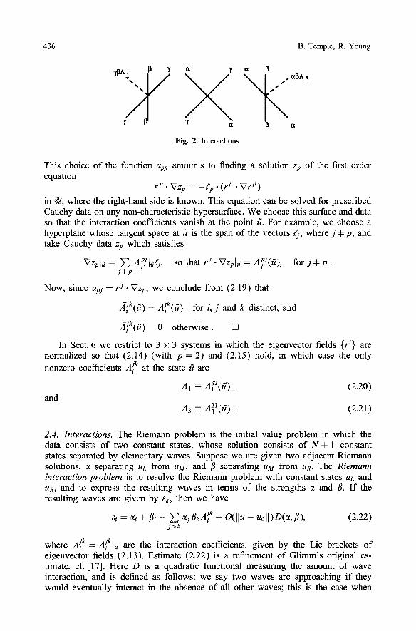
Fig. 2. Interactions

This choice o f the function ape amounts to finding a solution zp o f the first order equation

r p . VZp = --~p, (r p . ~ r p)

in q/, where the right-hand side is known. This equation can be solved for prescribed Cauchy data on any non-characteristic hypersurface. We choose this surface and data so that the interaction coefficients vanish at the point ~. For example, we choose a hyperplane whose tangent space at ~ is the span of the vectors dj, where j 4: p, and take Cauchy data zp which satisfies

VZp[a = ~ APpJ[adj, so that rJ .Vzpla = aPpJ(~), f o r j 4 : p . j4=p

Now, since apj = rJ. ~TZp, we conclude from (2.19) that

Ajk(~) = Ajk(~) for i, j and k distinct, and

AJik(~) = 0 otherwise. []

In Sect. 6 we restrict to 3 • 3 systems in which the eigenvector fields {r i} are

normalized so that (2.14) (with p = 2) and (2.15) hold, in which case the only

nonzero coefficients A j~ at the state ~ are

A1 - a~2(~) , (2.20) and

A3 - Azi(~) �9 (2.21)

2.4. Interactions. The Riemann problem is the initial value problem in which the data consists of two constant states, whose solution consists o f N § 1 constant states separated by elementary waves. Suppose we are given two adjacent Riemann solutions, ~ separating uL from UM, and fl separating uM from uR. The Riemann interaction problem is to resolve the Riemann problem with constant states uL and uR, and to express the resuking waves in terms of the strengths a and ft. I f the resulting waves are given by ek, then we have

I~i = ~i § fli § ~ O~jflk hjk § O(llu - u 0 1 l ) o ( ~ , f l ) , (2.22) j>k

where A jk jk = Ai la are the interaction coefficients, given by the Lie brackets o f eigenvector fields (2.13). Estimate (2.22) is a refinement of Gl imm's original estimate, cf. [17]. Here D is a quadratic functional measuring the amount of wave interaction, and is defined as follows: we say two waves are approaching if they would eventually interact in the absence of all other waves; this is the case when


the wave starting on the left is in the faster family, or both waves are in the same family and one of them is a shock. The amount of interaction D is then defined by

D(a, fl) = ~ ICtpI3ql , (2.23) App

the sum being over all approaching pairs of waves. Note that all second order terms in the estimate (2.22) appear in D, so that

ei = ~i + fli + O ( D ) , (2.24)

and moreover the coefficients A jk in (2.22) can be evaluated at the origin ~ rather than at the specific states UL, etc.

Restricting to 3 • 3 systems possessing a Riemaun coordinate, we assume that A1 and A3 given by (2.20) and (2.21) are the only nonzero interaction coefficients at the state ~. With these simplifying assumptions, we can represent the interactions which occur schematically, with all strengths of outgoing waves given to within a third order error, as in Fig. 2. We again mention the fact that no new entropy waves are generated to leading order. This observation will be crucial in Sects. 6 and 7, and indeed it is known that without some assumption being made, solutions can explode in amplitude in finite time, [5, 18].

3. The Method of Reorderings

We recall the method of reorderings and define the nonlinear functionals which will be used to bound the oscillation and total variation of the Glimm approximants. The main idea in Glimm's analysis is to build a decreasing potential which measures the errors produced from future interactions. For initial data having small total variation, this potential was constructed by Glimm, and was shown to be bounded by the square of the total variation. Similarly, in case there is a coordinate system of Riemann invariants, a quadratic functional is sufficient.

However, in general systems of three or more equations, when the initial total variation is large, the quadratic effects of interactions become important and lead to a variety of destabilizing phenomena. In this case we must update the potential for interaction effects as new waves are scattered by earlier interactions.

It is enough to consider only quadratic effects, as these control higher order effects. It is important to note, however, that for general systems, it is not possible to bound the quadratic effects, and the solution may grow unboundedly unless restrictions are placed on the Lie algebra of eigenvector fields. Our discussion is general, but the notation for the interaction maps is developed in Sect. 3.2 only for 3 • 3 systems possessing a Riemann coordinate.

3.1. Reorderings. We briefly recall the theory of reorderings introduced in [17], and use these to build the nonlinear functionals. Our notation is as follows: we suppose that the mesh-size Ax is fixed, and consider the Glimm approximation corresponding to this mesh-size on a given spacelike/-curve. By finite speed of propagation we assume without loss of generality that the approximation is compactly supported. The approximation then consists of a sequence of constant states {u0,..., u , } , each


pair o f states being separated by a single wave. We shall refer to the wave sequence 7 = (71,. . . , Vn), where the wave Yi separates the states ui-1 and ui. I f 7i is a ci-wave, we say that (Cl . . . . . Cn) is the index o f the wave sequence. The index ci identifies the family o f Yi, so that the wave strength determines the wave completely; for this reason we do not distinguish between the wave and its strength.

We shall model the evolution o f the Glimm approximation through changes in this wave sequence, as follows. The propagation and interaction o f waves correspond to changes in the order of the wave sequence, and consequent changes in the strengths o f the individual waves. We shall model these phenomena in an abstract setting, thus reducing the problem to an algebraic one. The symmetric group S, acts on the waves by permuting them, and we shall also allow waves to merge. This allows us to more accurately capture interaction errors and nonlinear decay, while requiring more care in definitions. We shall first consider a large class of maps, and then restrict to those which are admissible, both from a physical point of view, and as determined by Glimm's scheme.

A surjective map ~: {1 . . . . . n} ~ {1 . . . . . m} defines an action on sequences of n waves through permutation of subscripts. That is, the map z acts on the wave sequence ~ = (71 . . . . . 7,) by shifting the wave 7i from position i to position z(i). I f the new sequence is 5 = ~(7), we have 6~(i) ~ 7i, these being equal at the linear level. We say the map z reorders, or is a reordering of, the sequence 7. We similarly define the action o f z on the index c = c(7) by permutation o f subscripts. In order for the reordered index to be single-valued, we shall require that if z(i) = -c(j), then ci = cj. This corresponds to the collapse of two waves o f the same family into a single wave. Note that an abstract reordering keeps track o f the possible future relative positions o f the original waves, but does not tell us actual positions, nor how the strengths o f these waves change.

We can define a composition of maps as long as we take care that domains and ranges match up correctly, for example, if z maps n numbers to m and a maps m numbers to p, then the composition a r is a well-defined map of n numbers to p. In the sequel we shall implicitly regard all compositions as consistent, without further regard for the domains o f maps.

The permutation z identifies the positions o f the reordered waves, but also carries information about the interactions that must have occurred in reordering the waves. In order to get at this structure, we define the crossing set C, by

C~ = {( j ,k ) I J < k and z ( j ) > ~(k)},

so that C~ identifies the initial positions o f those pairs of waves which will cross under the action o f v. Similarly, since our maps are not necessarily injective, we identify the merge set

M~ = {( j ,k) I J < k and ~(j) = ~ (k ) ) ,

consisting o f those pairs of waves which are joined under the action of ~. It is convenient to define the interaction set I~ as the union of crossing and merge sets. We extend the action o f a, and refer to the pre-image under a of C, as

a'C~ = { ( j , k ) l ( a j , ~ k ) E C~},

with similar notation for other sets. We now isolate those maps which give rise to "physical" reorderings of waves.

Due to hyperbolicity, in order for a pair o f waves to cross, that is to pass through


each other, the wave on the left should travel faster than that on the right. Physically, waves in the same family may merge to form one wave, but never cross. Thus for a reordering z of the wave sequence Y, we require that in order for the waves 7j and 7k to cross (where j < k), the wave 7j should be in the faster family, while waves which merge should be in the same family. We express this symbolically as

Condition R: For every pair ( j , k) C C~, we must have cj > ck, (R) while i f ( j , k ) c M~, then cj : C k .

We say that the reordering ~ of 7 is admissible if it satisfies (R), and we write E A(y), where A(7) is the set o f all admissible reorderings of the sequence 7. We

note that the set A(7) is determined only by the index c = c(7) of the sequence, and does not depend on the strengths (or actual speeds) of the individual waves, so that any reordering admissible for the sequence Y is admissible for all sequences with the same index as Y. We now enumerate some of the properties of admissible reorderings, which can be derived directly from Condition (R) cf. [17].

The product o f admissible reorderings is admissible. Physically, once a pair of waves has crossed, these waves will diverge from each other, and any pair o f waves can cross or merge at most once. Given a composition of two admissible reorderings, we express the composite crossing and merge sets as

C,~ = C~ U v'C~, (3.1)

and g ~ = Ms U z 'M~, (3.2)

where U denotes a disjoint union. According to Condition (R), even though the inverse z~(j) o f j is not well-

defined, its index G'(j) is. This enables us to check admissibility of a map a of the reordered sequence z(7), by verifying that i f ( j , k ) c I~, then either c.d(j) > c.ct(k ) or ee(j) = ce(k), as appropriate.

In order for a pair o f waves to cross or merge, all waves between them initially must cross or merge with one of them before they can interact. That is, only adjacent pairs o f waves may cross or merge, and any admissible reordering consists of a series of pairwise interactions of adjacent pairs o f single waves. This observation allows us to factor reorderings into admissible pairwise interactions.

We have two types of pairwise interactions, namely transpositions and joins. The transposition K = (k : k + 1) flips k and k + 1 while leaving all other places fixed, while the join ~b p maps positions p and p + 1 back to p, and adjusts the other positions accordingly. Thus ~P(i) = i - 1 for i > p , and other places are left fixed. In order for these pairwise interactions to be admissible, we require ek > ek+l or ep = Cp+l, respectively. Note that each join contributes to the merge set only, while each transposition contributes to the crossing set only, that is

I o = M o and I x = C ~ ,

while C~ = M~ = (~. In particular, joins do not contribute to crossing sets, although they may cause the labels o f crossing waves to change.

We shall factor our reorderings into products o f these pairwise interactions, and will make heavy use of induction when considering arbitrary reorderings. Note that this factorization is not unique, and indeed we shall consider maps with different (admissible) factorizations to be distinct as reorderings. Thus each reordering has an implicitly given factorization.


Each factorization of the reordering tr = 2 s " " 21, where each 2r is a join or transposition, determines a time-like ordering on the interaction set Io, as follows. We say the pair ( i , j ) interacts before the pair (k, l), and write ( i , j ) ~ (k, l), if there is a reordering p, defined by # = 2m.. . 21 for some m, under which the pair ( i , j ) interacts, but under which the pair (k, l) does not interact. That is, ( i , j ) ~ (k, l) if ( i , j ) C 1~, while (k, l) @ 1~. The factorization may be recovered by specifying an order relation on the set I~. We cannot, however, arbitrarily order the crossing set I~, for Condition (R) implies that certain wave pairs will always cross before others.

Corresponding to each crossing pair ( i , j ) E I~ of the factored reordering o" = 2 s �9 " - 21, we associate a "subordering" # of a, as follows. We set # to be the largest reordering # -- 2m"" 21, under which the pair ( i , j ) does not interact. Thus if/~ is associated to (i , j) , and we set 2 = 2re+l, then the pair ( i , j ) interacts under the product 2#, and in fact we must have #(i) + 1 = #( j ) , and I~ -- {#(i,j)}. With this notation, we see that (k, l ) ~ ( i , j ) if and only if (k, l ) E I t. For the product n = az of factored reorderings, it is clear that ( i , j ) ~ zP(k, l), for each (i , j) E I~ and (k, 1) E I~, and the relation ,~ extends the order relations defined by the factorizations of a and z, respectively. We note that not all interacting pairs are comparable: indeed, if ( j , k ) c Me, and (zi, z j ) c Ca, then both ( i , j ) and (i ,k) E C~, but these cannot be compared under %~.

As was noted in [17], reorderings respect consecutive subsequences, so that there is a space-like ordering principle for waves generated by interactions with a fixed wave, namely the order is preserved or reversed. Other properties of reorderings mentioned in [17] are also valid here. Although the present definition of a reordering is slightly more general than was used in [17], our claims are straightforward applications of Condition (R), and more details can be found there.

3.2. Interaction Maps. We now recall the definition of interaction maps, making some changes for our particular assumptions. When two waves of different families interact, they generate waves of other families. This effect is accounted for by changing the strength of a nearby wave in the corresponding family. Interaction maps keep track of the waves whose strengths change as a result of the interaction. Thus given a factored reordering tr, an interaction map z~ acts on the crossing set C~ as follows: the integer z~ refers to the wave whose strength is changed due to the interaction of the waves 7j and 7k. We are using reorderings and interaction maps to model quadratic effects only, and so at this stage will ignore all cubic and higher-order effects, and treat quadratic effects as exact.

To simplify the notation, we describe the interaction maps for the class of 3 • 3 systems possessing a Riemann coordinate. We refer to this field as the entropy field, and to the others as acoustic fields. With this assumption, the only quadratic effects of interactions that arise come from the interaction of sound waves (i.e. 1- and 3-waves) with entropy changes (2-waves): in this case the affected wave is simply the nearest sound wave of the third family. We remark that although this assumption simplifies our notation and definitions somewhat, it is not necessary for the construction: see [17] for the general construction for systems of N equations.

Before defining interaction maps, we consider in detail what happens inside a diamond. Here we assume that our sampling is random in time, but uniform in space. Suppose for definiteness that a 3-wave enters the diamond from the left, and this is about to interact with a 2-wave entering the same diamond, see Fig. 3. Then the 2-wave must enter the diamond from the right, and moreover there must be a


Fig. 3. A Single Diamond

1-wave (possibly of zero strength) entering the diamond between these two waves, also from the right. Thus the 3-wave first crosses the 1-wave, with no quadratic effects, and then interacts with the 2-wave, reflecting a quadratic 1-wave to the right of the original 1-wave. Up to third order, the effect of random sampling is to combine these waves linearly into a single Riemann solution emanating from the center of the diamond. For our purposes, we note that the newly generated 1-wave is combined with the first 1-wave to the left of the interacting pair at the time of interaction. Similar remarks hold for other interactions.

Using the intuition from the argument above, we now define the interaction maps. Suppose that we are given a factored reordering o, which in turn determines an ordering 4o on the interaction set I~. Corresponding to each pair ( i , j ) E 1,~, we associate a subordering #. We note that quadratic effects are generated only by pairs of waves that cross, and moreover, interactions between pairs of sound waves (i.e. 3-waves with 1-waves) generate only cubic effects, and can thus be ignored. We therefore define the interaction map ~~ action on those wave pairs in the crossing set Co which include a 2-wave only.

In contrast to [17], we shall define interaction maps explicitly, and check that they satisfy the desired conditions. Thus, given a crossing pair (j, k) E C~, we let # be its associated reordering, and define

max{/I ci = ~, # ( i ) < # ( j ) } , zz (J ' k ) = m i n { i l c i = C,,u(k) < #(i)},

i f ~ = 1, (3.3)

i f ~ = 3 ,

where ~ E {1,3} is the index of the third (acoustic) family, which is affected by but is not part of the interaction. This defines the interaction map for those pairs of interacting waves which generate quadratic effects. We note that since our definition is explicit, a factored reordering has a uniquely defined interaction map, in contrast to the general case described in [17], where several interaction maps may be associated to a single factorization.

We now check that interaction maps as defined here satisfy the conditions stated in [17]. It is evident from our definition that the interaction maps defined here satisfy conditions (i) to (iv) stated in [17], when appropriately interpreted. These conditions imply that interaction maps respect the order of waves, so that those waves generated by the interaction of consecutive waves of one family with a fixed wave are also consecutive. The other condition concerned interaction maps for those


reorderings which are compositions: in this case the condition is not identical, since our reorderings are not invertible. The correct condition in this context is as follows. Recall that C~ = C~ U z'C~, and suppose that interaction maps ~, z ~ and ~ have been defined according to the above definition. Then we have

~~ = z~ on C~, (3.4) and

"cz ~z = zG'c on z'CG, (3.5)

which holds because our definition of z~(j , k) relies only on the associated reordering #, which is well-defined for each interacting pair. Of course, these statements make sense only for those wave pairs on which the interaction maps are defined.

We remark that instead of defining the interaction maps explicitly as we have done, we could have defined them by (backwards) induction, as in [17]. An inductive definition requires a choice, because reorderings are no longer invertible. However, if we require (3.3) to hold for transpositions, then Condition (R) and (3.5) fully determine the composite interaction map, leading to the above definition.

3.3. Changes in Wave Strengths. Now that we have defined interaction maps, which identify those waves whose strengths are affected by the interaction of nearby waves, it remains to give a detailed description of the changes in wave strengths due to specific reorderings. We shall describe these changes inductively, and later derive a compact formula for general reorderings. We are interested only in quadratic effects, and so shall ignore anything that is cubic or higher order in wave strengths.

Our notation is as follows: we start with a sequence 7 -- (71, . . . ,7,) of waves, with index c = (c l , . . . , On). Then the class A(7 ) of admissible (factored) reorderings is determined by e, and we suppose we are given some admissible reordering, say z. This has the interaction map ~ associated to it, as described above. We shall now describe the reordered sequence 6 = z(?) consisting of the waves in new positions and with strengths adjusted appropriately. We remark that the index d = z(c) is already known, namely dk = G'k, which is well-defined by (R).

Recall that we are implicitly assuming that each reordering is factored, and indeed~ different factorizations lead to different results. In order to proceed with the induction, we first describe the effects of a single pairwise interaction.

Consider the single join q5 = qSP. As described earlier, this models the merging of two waves from the same family into one wave. The effect o f two nonlinear waves from the same family interacting is to add their strengths linearly, with errors of third order. Thus, since we are ignoring cubic effects, we shall simply add the wave strengths. The two waves to be merged are 7p and 7p+1. I f 6 = q5(7 ) is the reordered sequence, we have

6p = "~p --~ ])p+l, (3.6) and

6O(j) = ?j, for j =~ p, p + 1. (3.7)

We now consider a transposition, which models the interaction of two waves from different families. According to our normalization, the incident waves themselves are not affected (except for cubic errors). The effect of the interaction is to generate a new wave in the third family, whose strength is the product of incident wave strengths, appropriately weighted. Since we are assuming that the second family has a Riemann coordinate, there are no new 2-waves generated. This was anticipated in our definition of interaction maps, and simplifies the notation. For


the definitions in full generality, see [17]. For other families, we do not allow new waves to be created, but instead adjust the strength of the nearest wave of the correct family, as described by the interaction map. This is exactly the effect of sampling in Glimm's scheme, as can be seen in Fig. 3, and corresponds to "conservation of the number of waves."

We again start with the sequence 7, and let the transposition be given by ~c = ( k : k + 1), and we shall describe the reordered sequence ~ = x(7). Let i = z~(k, k + 1) refer to the wave whose strength is affected by the interaction, noting that ci is that family distinct from those of the interacting waves, namely ck and ck+l. Then, since we are modelling only quadratic terms, we have

~)tr = ~)i "~ AciTk~k+l, (3.8) and

6,~(j) = ~j, for j # i . (3.9)

Note that apart from adjusting the strength of 7i by the Lie bracket term, we have also switched the relative positions of ?k and 7k+l, as required. In particular, if we assume the existence of a 2-Riemann coordinate, we have A2 = 0, so the transposition of a 3- and 1-wave pair has no effect on wave strengths.

We now inductively define the reordered wave sequence a(7) for an arbitrary reordering a. Since a is a factored reordering, we may write a = 2s . . . 21, where each 2j is either a join or transposition. We simply define

o(~) = ~ ( . . . (,~1(~))),

where each successive step has been described above. Although this definition is unwieldly for reorderings in general systems, we shall

see that in our case it leads to a manageable expression in terms of path integrals. The advantage in this definition is that it yields an exact expression at the quadratic level, in the sense that if local interactions were exact at second order, then this formula would be exact. By contrast, in [17], by considering second order terms in initial waves only, we get an approximation after two interactions (dropping brackets of brackets), and the errors so generated become significant when the total variation is large.

Again, we emphasize that although we have defined the reordered wave sequence for special systems, our definitions hold for general systems of N equations. However, without some assumptions on the interaction coefficients Ai, the reordered sequences become difficult to work with. Knowing that some solutions blow up, we must make some assumptions on the interaction coefficients to obtain bounds.

4. The Functionals

In this section we define the nonlinear Glimm functionals and describe the problems of continuity and boundedness of these functionals. Our aim is to describe the total variation and sup-norm of the Glimm approximation at large times. Recall that these approximations are represented at any time step, or, more generally, on any space- like 1-curve, as a sequence of waves. We shall define the nonlinear functionals in terms of these wave sequences and their reorderings. To obtain bounds on norms at large times, we must bound the functionals. The functionals include quadratic effects, and in order to get estimates which include all other nonlinear effects, we will need a continuity property for the functionals.


4.1. The Classical Induction. Before describing the functionals and their properties in detail, we briefly recall Glimm's original argument for bounding the total variation of the approximate solutions. Given a spacelike curve J, we define the total variation and error potential by

V(J) = ~ l ~ j l , and O(J) = y~ I~j[l~kl, App

respectively. Here the ~j 's range over waves crossing the curve J , and the second sum is over approaching wave pairs, that is those which will interact at some later time. The local error Q(A)= D(A) for waves entering a diamond is described similarly.

Since wave pairs interact once only, for any space-like curve J , we have

Q(J) <= V(J) 2 ,

which we refer to as boundedness of the functional Q (in terms of V). For the induction step, we argue as follows, referring to Fig. 1 for notation. The

waves entering the diamond A combine linearly in each family, up to a quadratic error which is bounded by D(A). Thus we have

V(J+) <= V(J_) -I- OlD(A), (4.1)

where c is some generic constant depending only on the conservation law. We view this as a statement of the continuity of V. The corresponding statement for Q is more interesting. First, there are fewer approaching waves crossing J+, as some waves have crossed inside the diamond. This means that there are fewer terms in Q(J+), and indeed the missing terms appear in Q(A). Thus we would like to write

"O(J+) + Q(A) = Q(J_ ) ." (4.2)

However, this relation is not exact, as some of the waves have changed due to the interactions in the diamond, so that Q(J+) is defined using waves of different strengths. We are thus led to a question of continuity: namely, if we change wave strengths locally (at a single diamond), what is the change in the global functional Q ? Glimm argued that since each wave approaches a subset of all other waves, and those waves leaving a single diamond may not interact, the total error in Q is the difference in wave strength multiplied by V, and so obtained the inequality

Q(J+) <= Q(J_) - Q(A) + czD(A)V(J_), (4.3)

where D(A) = Q(A) bounds the difference in wave strength. We combine (4.1) and (4.3) by induction: if V(J_) is small enough, say V(J_) < 1/2cz, then

V(J+ ) + 2Cl Q(J+ ) < V(J_ ) + 2Cl G(J_ ),

so this functional is decreasing. Thus we have the bound

V(J+) < V(J+)+ ZcaQ(J+) < V(Jo)+ ZclQ(Jo) < V0(1 +2ClV0),

and if V0 is small enough, then the inductive hypothesis is satisfied and we get total variation bounds, as required. In the sequel we will define Q* to be an extension of Q which includes cumulative quadratic effects in such a way that (4.2) holds


exactly at the quadratic level, and the higher order errors due to interaction will be estimated by the continuity properties of the fimctional Q*.

4.2. Definition of the Functionals. The above argument required V0 to be small to get bounds on the total variation for large times. To get results for large total variation, we must more accurately describe the effects of interactions by taking quadratic effects into account. We will use the method of reorderings to do so. In [17], we constructed a potential P for the sup-norm, which included (some) quadratic effects. In that paper, the boundedness and continuity of this functional P were discussed, without identifying them as such. Here we shall describe analogous functionals V* and Q* for the total variation and the quadratic error potential, respectively. Our notation will be that the * indicates that the functional is the usual functional with cumulative quadratic effects included. For convenience we will assume the existence of a 2-Riemann coordinate, although the functionals can be defined for general systems.

In Sect. 2.2 we described the total variation, sup-norm and local d-variation of a sequence of constant states separated by waves. We shall similarly define all other ftmctionals in terms of these wave sequences, and the extension to space- like curves is then clear, namely taking the supremum over all (consecutive) wave sequences crossing that curve. Thus we suppose that we are given a wave sequence

= (71 . . . . . Vn), together with the associated machinery of reorderings described earlier.

Since we know that time-independent bounds are not available, we shall implicitly fix a time T of existence, and restrict the class of reorderings appropriately. That is, we admit only those reorderings corresponding to interactions taking place up to time T. Thus, because the system is hyperbolic, certain pairs of waves (initially very far apart) will not cross in time T, even though they are approaching. Note that the number of interacting pairs still depends on the mesh size. Henceforth the class of reorderings will be restricted to interactions taking place before time T, and we shall make the dependence on T explicit only when convenient.

In [17], we defined the action of a reordering on a wave sequence, and then defined the potential P as the supremum of the sup-norm of reordered sequences, over all reorderings. That is, we defined a new wave sequence z~, and defined

P(7) = sup S(z*7), "C

the sup being taken over all admissible reorderings and interaction maps. Note that the sequence zz7 is not the same as the sequence z7 described in this paper, as the present treatment includes cumulative quadratic effects (brackets of brackets).

Our potential for the total variation is analogously defined as the supremum over reorderings of the variation of the reordered sequence,

v*(7) = sup v(~7) ,

Note that our construction included quadratic effects, and so the functional V* should describe the total variation at large times, except for (accumulated) cubic errors. We know that local cubic errors are controlled by quadratic terms, and continuity of the functional V* will allow us to control the cumulative cubic errors.

We will use the local variation of the entropy of the solution in our estimates, and so we need a functional that measures this quantity. Since entropy jumps


are represented by 2-waves, we define a functional H which measures the local d-variation by

H(7) = sup ~ I~il, (4.4) io,i d Ci=2

where the sum is over 2-waves between i0 and id, and the supremum is over indices chosen such that 7i0 and 7id are at most distance d apart in the approximation. This quantity is bounded by Ilwlld, if we define the strengths of each 2-wave as the entropy jump across that wave. Moreover, the fact that entropy is a Riemann coordinate implies that 2-waves undergo only cubic errors in wave interactions. In terms of reorderings, this means that the only elementary interactions resulting in changes in 2-wave strengths are merges of 2-waves, which do not increase the local 2-variation. Thus for any reordering z, we have H(zT) < H(7). We emphasize that this functional has this special property only for systems possessing a Riemann coordinate.

Finally, we must define the quadratic error potential. As in Glimm's original construction, we wish to define a functional that decreases across a diamond, so that this decrease balances the increase in norms due to interaction error. The local interaction error is given by O(1)D at quadratic level and O(1 )SD when quadratic terms are included (see (2.22)). Moreover, our error potential Q* should reduce to D for local interactions, as does Q. We know that when considering the Glimm error potential Q, the error term involving V (and forcing V to be small) appeared when we were considering continuity of Q. We thus look for a functional Q* satisfying a similar functional equation (4.2), but with better continuity properties.

The contribution to the error potential due to a pair of waves interacting is the product of their strengths. This product of strengths appears as a term in Q. However, the error appears only when the pair actually interacts, and at the time of interaction, these strengths will have been changed by earlier interactions. We thus build the functional Q* by again taking products of wave strengths, but measuring them at the time of interaction, rather than initially. This is accomplished via the method of reorderings, as follows.

Suppose we are given a reordering z of the sequence 7. Then the set I~ determines which wave pairs interact, and thus which terms should appear in Q*. We now find the strength of the waves at the time of interaction. To each interacting pair (j , k) E L, we associated the "sub-ordering" # of z. The strengths of the waves 7j and 7k when this pair interacts, are just the corresponding strengths in the partially reordered sequence/~(7). Note that this is consistent with our inductive definition of the reordered wave sequence.

We are now in a position to define the functional Q*. With notation as above, we denote by 7~ and 72 the reordered waves 7j and ?k before they interact, that is

7~ = q jr and ?~ = r/k,,

where j l = p( j ) , U = #(k) and q = p(?) is the partially reordered sequence. Note that the partial reordering/~ is defined for all interacting wave pairs, and is different for each interacting pair. We now define

Q*(?,r) = E j k - - - -E j k + 17)117kl App C~ M~

where the ~ on the second sum indicates that the sum is over approaching waves only, that is those for which one of ?~'. and 7~ (with c] = ck) is negative. This is the usual property that rarefaction waves of the same family produce no error. We also


impose the restriction that each interacting pair appear only once in the sum: thus if (k, I) E M s, so that both (j, k) E I~ and (j , 1) E 1~, and 7~ = 7~, the corresponding term t7~1t7~1 should not appear twice. Finally, define the quadratic error potential Q*(J) ~y

Q*(J) = sup Q*(7, z ) ,

where the sup is over all finite consecutive wave sequences 7 in J , and admissible factored reorderings z E A(7).

4.3. Properties of the Functionals. We now describe the algebraic relations for V* and Q* which will be used in the sequel, and describe in detail what we mean by continuity and boundedness. We wish to bound the functionals at later times by the initial functionals, if possible. In order to do this, we shall describe the change in functionals under a reordering, which corresponds to one or more diamonds. In describing the change in functionals, we shall see that our inductive definition of reordered wave sequences leads to exact functional relations, thus explicitly separating the continuity properties as described above.

To describe the change in functionals, we consider the composition of reorderings. Thus suppose that z E A(7), and let 6 = z(7) be the reordered sequence. Now if o-E A(6), the composition tTz is admissible for 7- According to our inductive description of reordered wave sequences, we have exactly

~(~) = G~(~),

and we use this to compare the functionals at different times. Since this relation holds for any ~ E A(6), we immediately find

v * ( ~ ) = v*(~7) _-< v * ( ~ ) ,

which says that the functional for the total variation does not increase with time. Note that here we are considering only quadratic terms, and so cubic errors have not yet been taken into account. We will need continuity of the functionals in order to deal with these cubic effects.

We now write down an algebraic relation for the quadratic error potential Q*. Using the same notation, we wish to compare Q*(6, ~) and Q*(7, o'z). Note that if/~ is associated to the interacting pair (zj, zk) E I~, then the sub-ordering associated to the corresponding pair (j , k) E C~ is #z, and indeed we have 6~j = 7~ ~, etc. Thus each term in Q*(6,tT) appears in Q*(7, tTz). Conversely, those terms in Q*(7,o-z) which do not appear in Q*(6, a) are exactly those which interact under z. Also, since the reordering associated to an interacting pair does not depend on later interactions, these terms are exactly those in Q*(7, z), and we have

Q*(7, t~z) = Q*(zT, iT) + Q*(7, ~). (4.5)

I f z is the reordering associated with a single diamond A between J_ and J+, and ~- is the reordering associated with changes between J+ and some later time T, we interpret this relation as Q*(J_) ,~ Q*(J+)+ Q*(A), so that the quadratic error potential does indeed decrease by the right amount. A more precise estimate can be stated once we have established continuity of the functionals.

Now that we have found the appropriate functional relations, which are exact at the quadratic level, we shall investigate what is needed to complete our induction argument. Since we will be bounding the fimctionals by their initial values, it is


clear that they must be bounded initially. Since the functional V* is a potential for the total variation, we require that it be bounded initially in terms of the variation V, whereas the functional P which bounds the sup-norm at later times, must be bounded by S.

Our induction is on diamonds (or reorderings) in the Glimm scheme, that is on series of interactions, each of which produces quadratic effects plus errors which are cubic. As we have noted, our functional relations are exact only at the quadratic level. Thus when applying our formalism to the Glimm approximations, we must account for these errors. We first informally describe how this is accomplished.

We model the interaction of waves inside a diamond by a reordering which adjusts the wave strengths to account for the quadratic effects. From our interaction estimate (2.22), we know that the cubic errors are bounded by O(SD), where the sup-norm S is small and we have control over D(A) ~ Q*(A). Thus suppose that 7 represents the waves entering a diamond, and a represents those leaving. We have that for some reordering p,

a = P(7) + O(1)S(7)D(A).

We have seen that we can compare the functionals defined on the sequences 7 and P(7), and would like to compare these to those defined on 6. Since P(7) and 5 are close, this is a problem of continuity of the functionals.

The continuity property of functionals can be described as follows: suppose that the wave sequences 6 and 6' have the same index, but the wave strengths differ in a single position, say p. We shall say that some functional B is continuous, if

We require that K~ be independent of the number of waves and mesh-size, while it may depend on norms of the solution or time. The requirement is that our estimates be uniform in mesh parameters, so that we can pass to the limit of Glimm approximations. Supposing that the sequences differ in one wave only is convenient and represents no restriction.

A similar remark holds for boundedncss: we would like to know that the functionals, which represent norms at future times, can be bounded in terms of initial quantities. Thus we would like to know that

B(a) < Bo(Vo, So, T, . . . ) ,

where the arguments of B0 are known initially, V0 = V(6), etc. Of course, these bounds should be appropriate, so a bound for the sup-norm potential P in terms of 110 alone would not be useful. We remark that in most circumstances, boundedness and continuity of fimctionals are equivalent, although they are conceptually different. In particular, if the bounds are smooth functions of norms, then the functionals are also continuous. This is just the statement that differentiable functions are Lipschitz continuous.

5. Existence of Solutions

We are now in a position to fill in the details of the existence theorem. We will make assumptions on the boundedness and continuity of the functionals, and then


derive our result. This means that the problem is essentially reduced to an algebraic one, namely finding bounds for the functionals which are described by finite sequences of waves. In the following sections, we find time-dependent bounds for the fimctionals, so that we get existence for arbitrarily large finite times. In general, any assumptions made in bounding the functionals translate to restrictions on the solution to the Cauchy problem. Throughout we assume implicitly that the sup-norm is small enough that all our estimates are uniform.

The bounds for the nonlinear functionals V* and Q* will depend on the time T of existence of solutions, as well as the total variation of the solution, and the local d-variation of the entropy. This local variation is measured in terms of the functional H defined earlier. For completeness, we shall make the time dependence explicit in the induction.

We use the notation developed earlier and state our assumptions in terms of the functionals. First, we assume the nonlinear functionals are bounded,

V*(7 ) < V~(V,T) and 0*(7) < * = = Qo(V,T), (5.1)

where Vo "~ and Q~) are increasing functions of their arguments, and V = V(7 ) is the total variation of the sequence 7. We note that in general these bounds also depend on other quantities, although we will not make them explicit here. Indeed, our bounds will depend on the lengthscale d, and corresponding sup- and d-norms. Next, we assume that these functionals are continuous,

V*(7) - V*(7') < Kv(V, T)I7 - 7'1 (5.2) and

Q*(7) - Q*(7') < KQ(V, T)I 7 - 7 '[ , (5.3)

for sequences 7 and 7' differing in one wave in each family, and having the same index. Again Kv and KQ are increasing functions of their arguments, and may depend on other quantities. We remark that these assumptions are equivalent when the bounds are smooth functions.

In [17] it was shown that the functional P for the supnorm is both continuous and bounded with explicit bounds, namely

P(7) <= S(7) + AS(7)V(7), and P(7) - P(Y') < Kp[~ - 7'1,

where Ke = O(1)V, and O(1) and A depend only on the conservation law. We shall also make use of Glimm's estimate

V(J+) <= V(J_) + AD(A). (5.4)

Theorem 1. Suppose that the nonlinear functionals satisfy boundedness and continuity properties (5.1)-(5.3). Then 9iven any T and Vo, there is an ~ > 0 such that if the initial data uo of the Cauchy problem (1.2) satisfies

Iluoll~ < ~ and TV(uo) < Vo,

then the conservation law admits a weak solution with bounded oscillation and total variation. Moreover, the total variation of the solution is bounded up to time T, with bound V~ + 0(~), and analo#ous bounds are available for other norms.

We remark that e is defined in terms of V0 and KQ, so that ~ --* 0 as V0 ~ ~ . In our analysis, KQ depends on time, so that we get solutions for arbitrarily large but finite times. That is, given any time T, we have e = e(Vo, T) and we have


existence up to time T. Similarly, any other assumptions which are made in finding KQ must be imposed on the initial data. In our case, we require that the entropy of the initial data has local variation.

Hw(uo)lld < ~ < 1/3A, for some d > 0 .

Here A = max{A jk} is the maximum of the nonzero interaction coefficients, and is determined by the flux. For clarity in the proof, we shall make the dependence on the local variation H ,~ [[w(u)lld of the entropy explicit.

Although our main application is to 3 x 3 systems having a Riemann coordinate, this theorem holds for general N x N systems, with appropriate modifica- tions. The functionals V* and Q* are again defined inductively on reorderings, and any restrictions made in finding bounds for V* and Q* must hold for the initial data.

Corollary 5.1. Boundedness and continuity of the functionals V* and Q* are sufficient conditions for existence of solutions to general N x N systems. That is, we can choose ~ > O, depending on the bounds, such that the conclusions of the theorem follow.

In general, such bounds are not available for large times when the total variation is large, and solutions are known to grow without bound, [5, 18]. Any restrictions used in finding the bounds for V* and Q* must again be imposed on the initial data and the solution.

Proof As usual, we proceed by induction on space-like /-curves. There are two steps, first comparing the functionals evaluated at successive /-curves, and then carrying out the induction. We use the notation of Sect. 2.1, so that curves J_ and J+ differ by a single diamond A, and J0 is the initial/-curve. Again, since we are anticipating time-dependent bounds, we restrict the class of admissible reorderings to those spanning the finite time T.

Referring to Fig. 1, we suppose that the waves crossing curve J_ form the sequence 7, and those crossing J+ are given by the sequence 6. Also, let the reordering

represent the interactions inside the diamond A. According to (2.22), the local error is O(1)SD(A), and we have

6 = ~(y) + O(1)S(?)D(A).

By this we mean that the sequences 6 and z(7 ) have the same index, and the wave strengths differ only in those waves leaving A, and in particular no pair of these waves approach, see [17].

Since the reordering ~ models the diamond A, we expect that the quadratic errors Q*(?, ~) and D(A) are comparable. In fact, the only difference between these is that in Q* we measure each quadratic term at the time of interaction. Since z is a local reordering modeling only a single diamond, there are a limited number of interactions, so that the difference between these is cubic, and we have

Q*(7,~) = D(A) + O(1)S(J_ )D(A) .

We wish to compare the functionals for the sequences 6 and ?, respectively. This in turn reduces to the continuity of the functionals, as follows. Consider the functional V*, which satisfies V*(~7) < V*(7). We know that the sequences v(7)


and 6 have the same index, and that a few of the individual wave strengths differ by O(SD). Then by continuity of V* in (5.2), we have

V*(6) - V*(vT) < K v ~ 16p - (~7)pl

< Kv 0(1 )S(J_ )D(A),

where O(1) is uniform in a neighborhood and depends only on the flux. Now V*(J+) = V*(6) for some sequence 6, and since the corresponding sequence 7 lies on J_, we have

V*(J+) < V*(~) + KvO(1)SD

< V*(J_) +KvO(1)SD, (5.5)

which is the desired comparison of V*(J+) and V*(J_). As similar relation holds for the sup-norm functional P, namely

P(J+ ) < P(7) + KeO(1)SD

< P(J_)(1 +KeO(1)D(A)) , (5.6)

for some sequence 3 and corresponding ~ C J_ , see [17]. We obtain a similar estimate for the change in the local variation H of the entropy. Since H is defined in terms of the 2-waves only, and wave interactions have no quadratic effects on 2-waves, we have

H(J+) <= H(J_) + KHSD , (5.7)

where KH depends only on the conservation law. We have implicitly used algebraic relations for V*,P and H, saying that these decrease at quadratic level after interaction.

We treat the quadratic error potential similarly: the error potential for J+ is given by Q*(6, a), where a is an arbitrary reordering of 6, representing wave interactions up to some later time. Given the corresponding sequence ~ C J - , we shall compare this to Q*(v7, a) by invoking the continuity (5.3) of Q*. We then use the functional relation (4.5) for Q* to compare that with Q*(~, av), which is in turn smaller than Q*(J_). Carrying out the details, we have:

Q*(b,a) < Q*(w,a )+ KQO(1)S(7)D(A)

< Q*(7, a~) - Q*(7, 3) + KQO(1 )S (JD(A) ,

which, when maximizing over a, leads to

Q*(J+ ) < Q*(J_ ) - D ( A ) ( 1 - O(1)KQS) , (5.8)

where we have used the local estimate Q*(%r). .~D(A). Thus we see that as long as S is small enough, the functional Q* decreases by some fraction of D.

We now proceed with the induction. The new feature of the induction is that the constants K depend on the solution, so we must choose the initial sup-norm

small enough that we get a uniform decrease in Q*. Our separation of the sup- and total variation norms, together with the small error in Q*, allows us to carry out the induction for large variation, as in [14]. In the local estimates above, we evaluated the K ' s at J_: as these are increasing functions of their arguments, we shall overestimate them in the induction. In order to simplify notation, we include all O(1) terms depending on the flux into the K's .


Given an initial total variation Vo, we set

O~ = Q~(Vo,2q; T) ,

where 2r/ is an upper bound for the local variation H, and define

W = Vo + 2AQ~ (5.9) and

M = (1 + AVo)e2Xeg-~, (5.10)

where we have set

Kp = Kp(W, Zt/; T) and KQ = KQ(W, Zrl; T ) .

We will show that

S(J) < MSo and V(J) < W

and H(J ) ~ 2q, as long as So is small enough and H0 < q. Choose the bound e > 0 for So small enough that

eMKQ < 1/2 and 2eMKI4Q~ < rl,

and suppose for the induction that

V ( J _ ) + ZAQ*(J_) < W , (5.11)

P(J_) < P(Jo)e 2KP(Q~-Q*(J-)) (5.12) and

H(J_ ) + 2SoMK~IQ*(J_ ) < 2q. (5.13)

These assumptions imply that S(J_ ) < P(Jo)e2Keg-~ < MSo. By (5.8) we have

Q*(J+ ) - Q*(J_ ) < - D ( A ) ( 1 - K Q M S o ) <= -D/Z , (5.14)

and so also D < 2(Q*(J_) - Q*(J+)). Then by (5.4), we have

V(J+)+ZAQ*(J+) < V ( J _ ) + Z A Q * ( J _ ) < W ,

and by (5.7),

H(J+ ) § 2SoMKHQ*(J+ ) < H(J_ ) § 2SoMKI4Q*(J_ ) < 2rl .

Similarly, by (5.6) and (5.14),

P(J+) <= P(J_)(1 + KpD)

< P(Jo)e2Ke(Q~-Q*(J- ))e2Kp(Q*(J_ ) - Q * ( J + ) ) ,

where we have used 1 + x < e x. This completes the inductive step, and we have the bounds

V(J+) < W and S(J+) < MSo,

and H(J+) < 2~l. We have not made use of the functional V* in proving existence of solutions.

Instead, V* gives us an estimate of the growth of the total variation of the solution. In particular, the dependence on time T of V* gives an upper bound for the growth of total variation, which in turn drives the growth in the other norms. To see this,


observe that we are overestimating V by adding the factor 2AQ*, which controls the local error AD in V. As we have seen, however, the local error in V* is KvSD, which is much smaller. Thus we can control the growth of V* by adding a smaller multiple of Q*. Indeed, letting c = 2Kv(W,2q; T)MSo and using the bounds found above, we have

V*(J+ ) + cQ*(J+ ) <= V*(J_ ) + KvSD + c(O*(J_ ) - 19/2)

< r*(J_)+cQ*(J_) ,

so that V(J+) < V~ + cQ~, where c contains the small factor So. Now we see that for small values of e, the total variation at later times is approximately given by the functional V*. Furthermore, a knowledge of the initial wave configuration and the (non-local) reordering corresponding to the union of all diamonds below J+ should give an accurate approximation for the actual variation along J+. It appears that one should be able describe the pointwise large-time behaviour of the solution in this way. []

6. The Path Integral

In order to apply the general theorems of Sect. 5 to a given system, one must obtain the boundedness and continuity properties (5.1)-(5.3) for the functionals in this case. In particular, these conditions must hold for special reasons because they fail when T is larger than the blowup time in a resonant system of type (1.2). We now obtain the estimates (5.1)-(5.3) for 3 x 3 systems possessing a Riemann coordinate. In this case, our growth rate bounds will be determined by the d-norm, supnorm and total variation norms of the initial data. Thus we assume the existence of a Riemann coordinate, and use this to express reordered sequences in terms of a path integral formula. Given a wave sequence and set of reorderings, we have seen how the strengths of these waves change under the interactions represented by that reordering. However, our description is thus far inductive, and the resulting quantities are difficult to analyze. Our assumption means that the entropy field decouples, and can be treated as static at the quadratic level. This simplification allows us to describe reordered sequences in terms of a path integral formula.

6.1. Paths in Reorderings. Our first task is to describe paths in the framework of reorderings. The cause of instability in our systems is the generation of new waves due to interactions, which is compounded when these new waves themselves interact and generate more waves. In our construction, the generation of new waves is avoided by adjusting the strengths of nearby waves, thus conserving the number of waves. We now address the question of how these changes of strength accumulate.

When a pair (j, k) of waves interact, we identify the wave Ti whose strength is to be adjusted via an interaction map, namely i = z~(j, k). The new (scattered) wave may now go on and interact with other waves, each time generating yet another wave. In our model we are merely adding each scattered wave strength to an existing wave: this means that those waves with which the scattered wave will interact are already known, namely they are those waves which interact with i = z~(j, k) after the pair ( j ,k) has interacted. We can now inductively describe a series of interactions, keeping track of the accumulated strength due to quadratic


i / \,, I ~ 1

\

I t

t i . . . . . . . . . 1 ~ ; , ~ [

k 2 k 1 k 3

Fig. 4. Scattering pattern with a single path

effects of these interactions. Figure 4 illustrates the scattering of a single sound wave, and a single path which is part of that pattern.

Given a wave sequence and (factored) reordering ~, which determines the interaction map z ~, we make the following definition of a scattering path, which describes the changing position of a sound wave or a (multiply) scattered sound wave as it interacts with contact discontinuities.

Definition 6.1. An r-path in ~ is' a set {(jp, kp) I 1 < p < r} C C~, satisfying

(jp-l,kp-1)<~z(jp, kp) and l ~ ( j p _ l , k p _ l ) = j p ,

for each p < r. We shall say that the path begins at j l and ends at z(j~+l) =-- ~t~(jr, kr). We analogously define a O-path to be any index i, and say that it starts at i and ends at r(i).

A path is thus a means of tracking the position at which an accumulation of interaction effects is concentrated. In this definition, the kp's represent the contact discontinuities (2-waves) which scatter the sound waves, while jp represents the sound wave which has been generated as the result of the previous p - 1 interactions. The kp's can be viewed as the relative positions of the contact waves which scatter the sound waves, although the actual position of the contact changes due to sampling shifts. We shall see that we can also extract the accumulated wave strength associated to the interactions represented by that path.

As usual, we have defined paths independent of the actual strengths of waves appearing in the sequence, so that only the index of the wave sequence is needed to determine the possible paths in any reordering. We remark that paths feature only members of the crossing set C~, as these are the only interactions which generate quadratic effects by generating reflected waves.

According to our assumptions and our definition of interaction maps, images under t ~ are 1- and 3-waves only. Thus in the above definition it is implicit that each kp (for p > 1 ) refers to a 2-wave, while jp refers to a 1- or 3-wave, altemating between these as p changes. We extend this convention to ( j l , kl ), so that all non- trivial paths start at the 1- or 3-waves YJl" We denote the set of all r-paths in beginning at p = j t and ending at q = z(j~+l) by H~(p, q, z).

As we have done previously, we now consider compositions of reorderings, and the paths associated to these. We would like to know that paths can be constructed


inductively, and that all paths can be obtained by a suitable local construction. The compound structure of paths is described in the following lemma. We shall use the symbol n~ to refer to an arbitrary path in T, so n~ C C~. Our notation is that used earlier, so r reorders the sequence 7, and a reorders T(7), and the composition aT makes sense.

Lemma 6.2. A path rc~ in az determines unique paths n~ and na in �9 and a, respectively, via the definitions

rc~ = na~ N C~, (6.1) and

na = Tna~ n Ca, (6.2)

respectively. We say that rca~ projects to rc~ and ~ca. Conversely, given paths rc~ and rca in T and a, respectively, such that rc~ starts at the end of rc~, we can always find a path rc~ in aT which projects to ~c~ and ~ .

We note that different paths in aT may project to the same paths in a and ~, in case ~ is not one-to-one. When convenient, we shall denote a path which projects to ~r~ and 7z~ by ~a o ~ .

Proof Suppose that the path ~ consists of {(jp, kp)ll <= p < s}. Since these pairs are ordered by %~, and all pairs in C~ cross before those in TtCa, there is a unique r such that ((jp, kp)ll < p < r} c C~, and this is the path n~. To get a path in o-, we must advance the other crossing pairs by T: thus {(Tjp, rkp)lr + 1 <= p < s} is a subset of Co, and that it forms a path follows immediately from the fact that Tt a~ = tat on r That these paths can be described in the above set notation is clear.

For the converse, we must be more careful, as the path rca~ is not uniquely defined in general. Suppose that 7z~ is given by ((jp, kp)]l < p < r}, and ~a C Ca is {(lq, mq)[ 1 ~ q < s}, with Tt~(jr, kr) = ll. We wish to construct a path na~ which projects to these paths. It is clear that we should just copy n~ initially, so it remains to extend na~ in a way that projects to 7ta. Since T is not necessarily one-to-one, there will be some choice involved, although the choice is restricted by the requirements for a path. For each q, choose k~+q E Tt(mq). These are the only choices we have, as each jp+l is determined inductively by jp+l = ta~(jp, kp). It remains to check that the path n~ = {(jp, kp)]l < p < r + s } projects back to ha. To see this, note that "c(kr+q)= mq and, by induction,

T( jp+ l ) = TlaZ(jp, kp ) = la('~jp, Tkp ) = la( lp-r, kp-r ) = lp-r+l .

This completes the proof of the lemma. []

In view of this lemma, we can describe the paths in a particular reordering by induction, after describing the paths for the elementary interactions, namely joins and transpositions. For a join q~ ---- q~p, there are no non-trivial paths: however, there are two 0-paths which end at the same point, namely {p} and {p + 1}. There is a single 1-path for the transposition tc = (k : k + 1), namely the path {(k, k + 1)) which coincides with the entire crossing set.

We emphasize the fact used in the above proof that any path is uniquely determined by the starting sound wave j l and the contact waves kp, for a given interaction map. Also note that the only choice in the path na~ came in the choice of the kr+q'S. In particular, if T is one-to-one on the k ' s (which are contacts), the


path rc~ = rc~ o rc~ is uniquely determined, and a knowledge of all paths in z and o-, respectively, gives a full description of the set of paths in az. In fact, by considering the gas dynamics equations in the Lagrangian formalism, (so 22 = 0), and sampling randomly in time only, we can ensure that this is always the case.

The results of the lemma can be interpreted in terms of the sets Hr as

Hr(j,i,~r'c) C_ UI-lr_s(k,i,~r) o Hs(j ,k, 'c) , (6.3) s,k

with equality when r is one-to-one on contacts (2-waves). This abstract statement says that all paths of length r in a t are built up of paths of length s in ~ concatenated with paths of length r - s in a. Note that the only restriction on the shorter paths is that the end of the first be the beginning of the second, but this could be in a number of different positions. Comparing (6.3) to the arithmetical relation

leads to a bound on the number of paths.

Corollary 6.3. I f the reordering z is one-to-one on contacts and spans N time-steps, then

where # I I r ( j , . , ~) denotes the number of r-paths in z, starting at any given j.

Proof According to our construction, there is only one 2-wave entering or leaving each diamond. Also, each sound wave passes through a single diamond at each time step, so that it interacts with at most one contact at that time step. This means that any contact with which a particular sound wave interacts can be tmiquely identified by the time of interaction. We extend this idea to count the total number of paths starting at a fixed point. Figure 4 illustrates this "projection" of interactions of a single sound wave and a path onto interaction times.

We wish to count the number of paths in �9 which begin at position j . Thus suppose {(jq, kq)} is a path, with j l = j . We know that the path is uniquely determined by the sound wave j l , which is given, and the positions kq of the 2-waves appearing in the path. Now, for each jq, we can uniquely identify a time step tq at which the crossing pair (jq, kq) interacts. We thus have a projection of the path onto an increasing sequence of time-steps tl < t2 < " ' ' < t~. Moreover, since only one contact enters each diamond, different paths lead to different projections. This means that the number of paths starting at j is bounded by the number of increasing interaction times 0 < tl < t2 < . . . < t~. Since each tq = qAt corresponds to an integer (counting time-steps), and there are at most N time-steps, we have

[]

We will later use a similar path-counting technique in obtaining bounds for the nonlinear functionals. Although we require that 2-waves do not merge in this proof, in finding bounds we will not require a one-to-one map from paths to sequences of interaction times.


6.2. Path Integral Formula. We now use the abstract paths to get a useful for- mulation of the wave strengths in the reordered sequence r(7). Recall that we are assuming the existence of a 2-Riemann coordinate, so that all images under interaction maps are either 1- or 3-waves. We now make the further simplifying assumption that 2-waves do not merge. This is true for gas dynamics as long as we use the Lagrangian formalism, for which the entropy has zero wave-speed. This assunaption for 2-waves allows us to treat perturbations in that family (i.e. entropy fluctuations) as a static background source for changes in sound waves, which is fixed in time.

We can make the statement that no 2-waves merge more precise by adding an extra requirement to Condition (R), namely that if the pair ( j , k ) E M~, then we must have cj = ck =~ 2. This extra condition further restricts the set o f admissible reorderings, but does not change any of our previous assertions in any way. Hence- forth we shall assume that this extra condition is satisfied implicitly. We remark THAT THIS assumption is merely technical, as allowing two 2-waves to remain adjacent in the scheme instead of merging merely increases the set of reorderings and paths, but this increase does not affect the functional bounds at all, as the variation o f the sequence never increases after a merge. A more formal analysis o f this idea can be found in [17].

Since our definition uses only the index of a wave sequence, a path tracks only the position of the scattered wave we are tracing. In order to fully describe interaction effects, we must also take the actual wave strengths into account. Before writing down the path integral formula, we consider the strength associated to a single path. Thus suppose we are given a path rc~ = { ( j p , kp ) } . This represents the wave generated as a result of the multiple interactions occurring in ~z~. We wish to find the strength contributed by this scattering path. As before, we assume that each ekp = 2, and take cjl = 3, say. We shall trace the strength of the scattered wave as the path is traversed, as in Fig. 4. Thus the original strength is ~Jl, and when this wave interacts with 7kl, the reflected wave has strength e (1) = 7j lTklA 1 . This reflected wave then interacts with wave 7k2, to produce e(2) = e(1)7k2A3. This process continues inductively, and after r interactions, say r even, the wave generated by this series o f interactions has strength

e(r) = g(r-1)7krA3 = 7jl 7kl "'" 7kr(A1A3 )r/2 .

This then is the amount of wave strength generated as a result o f the interactions represented by the path n~. In this calculation, we have used the fact that 2-waves 7kp do not change at all across interactions. This observation allows us to use the initial 2-wave strength at later times. Moreover, because there is a 2-Riemann invariant, interactions between 3- and 1-waves have no (quadratic) effect, which means that different scattering patterns combine linearly, leading to the path integral formula, stated in the following theorem.

Theorem 2. Given the wave sequence 7 = (71 . . . . . 7n) and factored reordering ~, let 6 = ~(7) be the reordered wave sequence. Then for any i, the reordered wave c~i is given by the path integral formula

r =- ~ 7j ~ A( i , r ) ~ 7 k l " " " ~)kr "

j r>=O H r ( j , i , ' c )


Here 11~(j, i, ~) is the collection o f all r-paths in ~ starting ja = j and ending at i = zz~(j~,k~), and the weight A( i , r ) is given by

A( i , r ) = A[(~+U/2]A[r/2] where c = cz,i and c' = 4 - c c c / ,

We remark that this formula is applicable for all waves, although it is highly redundant for 2-waves. Indeed, no non-trivial paths end at 2-waves, and these do not merge, so that 8-ri = ~i for 2-waves. Merges of sound waves are also implicit in the formula, as paths corresponding to merged waves end at the same place. The weight A(i, r) consists of r = [(r + 1)/2] § [r/2] factors A, each corresponding to one reflection, and does not depend on the particular choice of path.

Proof The proof is by induction on the factors of the reordering z -- )].t" �9 �9 )q. I f is a single join q5 = qSq, then there are no non-trivial paths, and the 0-paths {q} and {q + 1 } end at q, while other 0-paths {j} end at ~b(j). The formula then reduces to the definition o f the sequence ~b(y). Similarly, i f ~ is a transposition tc = (k : k + 1), all 0-paths {j} end at to(j), and the 1-path {(k ,k + 1)} ends at tci = i = tX(k,k + 1). Thus the formula reduces to 8k(j) = 7j for j + i , and 8i = T~c,i § YkYk+lAci, which is again the definition of the sequence x(~).

Now suppose that the path integral formula holds for z. We consider the compositions ~bq27 and xr separately. First consider the join ~b = q~q. Recall that ~b q maps q and q § 1 to q, and changes the positions of all other waves appropriately. I f a = r(y) is given by the path integral formula, we must describe the new sequence 8~= ~b(8)= ~br(?). First, for j # q , we have simply 8~. = 66,j, which is the sum over the sets H ( . , ~b~j,v). For the merged wave, we have 6q = 6q + 8q+1, which is the sum over both sets / 7 ( . , q , z ) and 1I( . , q + 1,~). In the set notation of (6.3), we can express the set o f paths in ~br as

H r ( p , j , dpz) = 11r(p,q~9, Z), for j # q , (6.4) and

11r (p , j , (~z) = 11r(p,q, z) U lIr (p ,q + 1 , r ) , (6.5)

for each starting position p. These are exactly the sets over which we sum to get the 8j.'s. Moreover, the terms which are being summed are not changed, so that the path integral formula holds for qSz.

We now consider the reordering ~c,, where tr = (k : k + 1). Again we suppose that 8 = z(y) is given by the path integral formula, and we wish to show that the same is true for 8' = to8 = ~cz(?). For j =t= l~(k, k + 1 ), we have 8 5. = 8n, j , while by (6.3), r-paths in ~cr ending at j are exactly those in ~ which end at x ' j , that is Hr(p, j , ~:r)= Hr(p, ~:'j,z). Again we sum the same terms, so the formula holds for those j # tX(k, k + 1).

It remains to check the path integral formula for the wave 8~, where ~c'i = i = z~(k, k + 1). According to the definition, we have

6~ = 8 i § 8 k 8 k + l A E ,

where ? = c~,i, and we must express this in terms of the ~'s. According to our assumptions, either 6k or 6k+1 must be a 2-wave, and the other a sound wave from the ?t family, where ~t = 4 - E. For definiteness, we suppose that 8k is the 2-wave, the other case being similar. Then 8k = ?r by induction. Also, the w a v e s ~i mad


6k+1 are given inductively by the path integral formula. Thus we have

6~ = 6i § ~)k+lYr, kAg

= E ~ Yjl~)kl ""TkrA(i, r) r>=O Hr( ~ ,i,'c)

+ 7~,kAe ~ ~ 7A 7k, "'" 7kr A(k + 1, r ) . r Hr (" , k+l , z )

(6.6)

(6.7)

(6.8)

By the remark following Lemma 6.2, any r-path in z which ends at position k + 1 extends to a unique (r + 1)-path in tcz. Since z is one-to-one on 2-waves, the (r + 1) st pair of this path must be the pair (t~(j,.,k,.),z'k) E C,~, and the extended path ends at i. Moreover, since 6k+1 is a 6'-wave and 6i is a Y-wave, we have

AeA(k + 1, r) = AcA [(~+l)/21Ae[r/2] = A(i, r + 1 ) .

Thus the second sum above is exactly the sum over paths in Kz which include the pair "d(k, k + 1) and end at i, while the first sum is over paths ending at i but not including the pair z'(k, k § 1). Since these are exactly all paths in ~cz which ends at i, the path integral formula holds for 6~, and the theorem is proved. []

7. The Functional Bounds

We now find time-dependent bounds for the nonlinear functionals for systems with a Riemann coordinate. By the results of Sect. 5, these bounds are all that are needed to deduce large-time existence of solutions. We shall derive the bounds in steps, first bounding the functional V*, and obtaining the bound for Q* and continuity of the functional as corollaries.

Before proceeding, we recall our assumptions in detail. We are assuming that the second (entropy) family possesses a Riemann coordinate, so that the second interaction coefficient A 31 vanishes. Denoting the Riemann coordinate by w �9 ~ / ~ R, the strength of a 2-wave (which is a contact discontinuity) is defined by

7 = w(uR) - w(uL), (7.1)

where UL and uR are the states on either side of the wave. In particular, given a sequence of constant states separated by waves, the strength of all 2-waves can be found through the Riemann coordinate w. For convenience, we also assume that the second family is linearly degenerate, so that no 2-waves merge. We shall see that our bounds, and hence conditions for existence, depend on the entropy of the initial data. This is not surprising, because the (degenerate) entropy field does not grow or decay to leading order, so that entropy jumps in the solution persist.

Our estimates will depend on the local variation of the entropy of the data, quantified by the d-norm defined earlier,

IIw(uo )lld = supTVix, x+a](uo ) , x

which we require to be small for some d > O. This is a weak assumption which simply says that the variation of the entropy is spread out over intervals of length d,


and so does not accumulate at any point. Since we are dealing with wave sequences only, we shall use the functional for the local d-variation of the sequence,

H(7 ) = sup ~ 17il, ci=2

where the sum (and sup) are over 2-waves positioned in an interval of length d. It is clear that H is bounded by [[w(u)[la. Throughout this section, we assume that d is a fixed positive number, and the local d-variation H is smaller than a constant determined only by the conservation law.

We begin by considering the functional V* for the total variation. Recall that V* is defined as the supremum of quantities V(W), where y is a wave sequence and z is an admissible reordering. We shall find a bound for V* by expressing the reordered sequence z7 in terms of the path integral formula, and bounding the total variation of this reordered sequence. Since our bounds are time-dependent, we further restrict the class of reorderings to those which correspond to wave configurations up to time T, which we fix for the rest of this section.

The idea of the proof is as follows: according to the path integral formula, the amount of scattered wave strength generated by a single wave is

7kl "'" 7krA( " , r) , fir

where we sum over all r-paths emanating from that wave. Now if each 7kr were bounded by/3, then this is bounded by

~(flA)r#Ilrr <= ~ ( N T ) (flA)r '

according to Corollary 6.3. Now using the binomial theorem, we get the bound (1 + t~A) Nr < exp(/~ANr). Although this bound depends on the mesh size through the number Nr of time-steps, we modify the method to obtain uniform bounds by accounting for the d-norm of the initial data. We know that when the variation is small, it does not grow. In particular, on the local lengthscale d, the local variation is small and growth will not occur. We therefore overestimate the amplification due to interactions on the small lengthscale d, and then combine these into the full lengthscale of the support of the solution, to bound the growth of the solution as above. Thus, instead of considering each 2-wave separately, we group them into "blocks" of size d, and u s e / / a s an estimate for the amount of wave strength generated by each block. The number of blocks is then Nr = O(T/d), and we obtain uniform bounds by the above argument.

We proceed with the details. Fix the total variation V = V(7), time of existence T, mesh size Ax = 2At, as well as the local total d-variation of entropy 6 = H(7 ). We restrict the class of reorderings to those corresponding to a set of diamonds lying below the curve t = T. We prove the following theorem which gives the growth bound for V*, and thus establishes the growth rate bound in Theorem 1 at the quadratic level.

Theorem 3. I f the sequence 7 is such that r / = H(7) satisfies

6Aq < 1/2, for some fixed d > 0 ,


then the functional V* is bounded,

V*(7) < V(y) + V(7)exp(8ArIT2/d ) .

In particular, this bound is uniform as the mesh size Ax ~ O.

Proo f Since V* is defined by V* = sup~ V(W), we choose a reordering z and look for a bound for the variation of the reordered sequence.

According to the path integral formula in Theorem 2, the reordered sequence 6 = z7 is given by

6i = ~ 7j ~ A( i , r ) ~ 7k~' ' 'Ykr, (7.2) j r~O Hr(j,i,z)

where Hr( j , i, z) is the collection of r-paths in z from j = j l to i = zl~(jr, kr), and A(i, r) = A[(r+I)/Z]A[r/2] We have V(zT) = V(6) = Y'~il6il, and rearranging the sum

C C ! �9

gives V(z~,) __< ~ I~jl ~ ~ 17k," Tkr]A r , (7.3)

j r>=O FIr(j, . ,z)

where now the sum is over all paths in r beginning at j , and we have set A = max{[Al 1, [A3I}. We shall find bound for each amplification fac tor

Aj = ~ ~ [Tk, " 7kr[ ar , (7.4) r > 1 17r(j, �9 ,T)

which measures the amount of total variation generated by multiple scattering of the sound wave 7j. The functional V* is then clearly bounded,

V*(T) < V(y)(1 + A ) ,

where A is the bound for the amplification factor. We first estimate the amplification factor due to a group of 2-waves having

small total variation: this will be used to estimate the contribution due to blocks of size 3d.

Claim. I f the total variation o f 2-waves appearing in Aj is small, that is ~klYklA < e < 1, then so is Aj,

8 Aj <

= 1 - e

To see this, we simply write

AS =< E (EITk, I A ) ' " ( E I ? k r I A ) r > l

8

r~l - - 1 - e

We will use this to over-estimate the contribution due to each block. We now partition paths into blocks, as follows. For a fixed sound wave ?j

located at some point xj of space, we partition the real line into (non-overlapping) intervals

I m = (xj + md, xj + (m + 1)d]

462

of length d. We also define the extended intervals

B. Temple, R. Young

1fro = (xj + (m - 1)d, xj + (m + 2)d], (7.5)

= Im-1U lm U Im+l (7.6)

of length 3d. We shall say that 7~ (or simply ki) lies in the interval Ira, if the spatial position of the wave 7ki is in I,n initially (i.e. before any wave interact).

Suppose we are given a single path starting at j , and determined by the set {kl, . . . , kr}, each ki referring to the corresponding 2-wave 7ki- We partition the path into blocks as follows. Let ml be such that kl lies in the interval lml. Define the first block B1 to be the maximal set of ki's such that kl , . . . ,kbl lie in the extended interval [ml. Now let m2 refer to the interval 1,,2 containing the first wave not in [,nl, that is kbx+l, see Fig. 5. Now define b2 and the block B2 to be the largest set

of ki's such that kbl+l . . . . . kbl+b z lie in [m2. Continuing this process, we partition the path into blocks Bl , . . . ,Bt, with the

following useful properties. All 2-waves in a single block lie in an interval of length 3d, and therefore have maximum total variation 36. We will thus be able to apply the above claim to each block, regardless of the number of waves in that block. Moreover, according to our construction, the distance between consecutive blocks is at least d. This will allow us to bound the number of blocks.

With these definitions in hand, we now reconsider the amplification factor Aj. By partitioning each path into blocks, we can rewrite

(7.7)

where ~ b i = r and each group of waves comes from block Bi. According to our construction, each block Bi comes from a set of waves occupying a spatial interval

r i

| |

Fig. 5. Decomposition into blocks


of length 3d, and so having local 3d-variation given by 36. We can thus apply the claim above and bound each of these terms,

ITkl "'" 7k~ Abel < _ _ 3 A 6 < 4A6 bl = 1 -- 3A3 = '

etc., since 3A6 < 1/4. Using this bound in (7.7) then gives

Aj < ~(4Af )e#Me,

where #Me is the number of ways of choosing ~ blocks B1 . . . . ,Be. Finally, we count the number of ways of choosing E blocks, using the method of

Corollary 6.3. Since block are separated in space by distance d, and wave-speeds are finite, it takes at least d/2 units of time to move between blocks. We again track the block by projecting to corresponding times of first interaction inside each block. Thus we must choose times tl < . . . < t~ < T, where each ti+l - ti > d/2. In Corollary 6.3, because each scattered wave had a known direction, the interaction times were enough to uniquely determine the path. In the present case, however, an even number of interactions in one block will not effect a direction change, so that there is a corresponding choice of direction for each interaction time (i.e. the next block could be either to the left or right of the present block). Thus the choices of E times together with d directions determine all possible ways of choosing blocks, and we have

#~e < ( T 2 / d ) 2 ~ =" ~ "

Thus we finally obtain a bound for the amplification factor,

< (1 + 8A6) rz/a (7.9)

< exp(8AfT2/d), (7.10)

where we have again used the binomial theorem. We note that this amplification factor is uniform in the mesh size. Finally, inserting this bound for the amplification factor into (7.3) yields the total variation bound, thus completing the proof. []

We remark that in bounding the amplification by partitioning paths into blocks, we have made heavy use of Lemma 6.2, which says that complex paths project to and are built up from smaller paths.

It is remarkable that the bound reduces to finding the amplification due to the passage of a single weak sound wave through a fluctuating entropy field, and that the amplification is essentially independent of the strength of the sound wave. The theorem shows that we have a bound for the variational potential V*. We shall use this to show that the quadratic error potential Q* is bounded, and the functionals V* and Q* are continuous.

Corollary 7.1. Under the assumptions of Theorem 3, the quadratic error potential Q* is also bounded, namely

Q*(7,z) < V 2 exp(16AfT2/d).


Note that this can be viewed as analogous to the bound for Glimm's quadratic error potential, Q < V 2, where we must now replace V by the potential V* for the variation.

Proof Given 7 and z, by Eq. (4.2) we have

cr Me

where the sub-ordering p is associated to the each pair (j , k) �9 C~. We now expand each 75 by the path integral formula, and rearrange the sum to get the bound. The idea is that since each wave pair interacts only once, and we can bound the amount of total variation generated by each wave, the total is bounded by the square of the variation bound. Using the path integral formula, we have

~ = Z v / E A ( k ~ r ) E ~rat'"Vmr, I r H r ( t , k, i t )

with the analogous formula for ~ . Now, since paths in tt are paths in ~, we have Hr(l,k,#) C Hr(l,k,z), so that we may use the amplification factor of the theorem to bound the total variation, even though the partial reordering # changes for different interacting pairs. Substituting in the bounds found above, we get

O*(7,z) < E [~11~1 (7.11) Ir

< ~ ly}lAi17tlAi (7.12) j , 1

< (7.13)

and the result follows. []

We now address the problem of continuity of the functionals. Starting with two sequences which differ in one wave only, and a fixed reordering, we must show that the resulting sequences differ by an appropriately small amount.

As above, we start with a sequence ~ and reordering z. We have seen that the reordered sequence 6 = v7 has bounded variation. We now wish to describe the effect of perturbing a single wave in the initial sequence. Thus, suppose that 7t is a sequence which coincides with 7 except in one position, say p. We wish to bound the differences V*(7) - V*(7 I) and Q*(7,z) - Q*(7',z) by a multiple of lTp -7p ] .

Corollary 7.2. The functionals V* and Q* are continuous: that is, there are functions Kv(V,H) and KQ(V,H), also dependin9 on time T, such that

IV*(y) - V*(~')[ < Kv(V,H)[~p - ~'pl, (7.14) and

[Q*(Y) - Q*(7')[ < KQ(V,H)IYp - 7pl. (7.15)

Proof Since the bound for the functional V* depends smoothly on the quantities H(y) and V(y), and these norms change by at most [7p - 7p], we have

0V* ~V* iV*(7) - V*(7') < --~v-]V(7) - v(v')[ + - ~ [ H ( 7 ) - H(7')[ (7.16)

< KF(V,H)lyp - Ypl, (7.17)


where KV is an increasing function of its arguments, and we have set

V = sup{V(7), V(?')} and H = sup{H(7 ) ,H(7 ' ) } .

It is clear that Q* is also continuous. []

Theorems 1 and 4 now follow from the general theorems of Sect. 5, using the bounds established in Theorem 3 and Corollaries 7.1 and 7.2, which are applicable to systems possessing a Riemann coordinate, which include the systems (1.1) and (1.11).

References

1. Cheverry, C.: Optique geometrique faiblement non linearire: Le cas general. Prepublication 95-11, Institut de Recherche Mathematique de Rennes, Mars 1995

2. Lax, P.D.: Hyperbolic systems of conservation laws, II. Comm. Pure Appl. Math. 10, 537-566 (1957)

3. Glimm, J.: Solutions in the large for nonlinear hyperbolic systems of equations. Comm. Pure Appl. Math. 18, 697-715 (1965)

4. Glimm, J., Lax, P.: Decay of solutions of systems of nonlinear hyperbolic conservation laws. Memoirs Amer. Math. Soc. 101 (1970)

5. Hunter, J.: Strongly nonlinear hyperbolic waves. Nonlinear Hyperbolic Equations-Theory, Computational Methods, and Applications, J. Ballman, R. Jeltsch (eds.) Viewig, 1989, pp. 257-268

6. Metivier, G., Joly, J.L., Ranch, J.: Resonant one dimensional non-linear geometrical optics. (to appear), 1992

7. Metivier, G.: A nonlinear instability for 3 x 3 systems of conservation laws. Preprint, 1993. 8. Liu, T.-P.: The deterministic version of the Glimm scheme. Commun. Math. Phys. 57, 135-148

(1977) 9. Majda, A., Rosales, R.: Resonantly interacting weakly nonlinear hyperbolic waves in a single

space variable. Stud. Appl. Math. 71, 149-179 (1984) 10. Schochet, S.: Glimm's Scheme for Systems with Almost-Planar Interactions. Commun, PDE,

16, 1423-1440 (1991) 11. Serre, D.: Richness and the classification of quasilinear hyperbolic system. IMA volumes

#29, Berlin, Heidelberg, New York: Springer, 1991, 315-333 12. S6vennec, B.: Geometfie des systemes de lois de conservation, Memoire SMF #56 (1994) 13. Smoller, J.: Shock-Waves and Reaction-Diffusion Equations. Berlin, Heidelberg, New York:

Springer 1983 14. Temple, J.B.: Supnorm estimates in Glimm's method. J. Diff. Eqn. 83, no. 1, 79-84 (1990) 15. Temple, B., Young, R.: The large time existence of periodic solutions for the compressible

Euler equations. To appear in Proceedings of the IV International Workshop on Shock Waves and Conservation Laws, IMPA Brazil, July 1995

16, Tong, Y.: A fimctional integral approach to shock wave solutions of Euler equations with spherical symmetry. Commun. Math. Phys., to appear

17. Young, R.: Sup-norm Stability for Glimm's Scheme. Comm. Pure Appl. Math. 46, 903-948 (1993)

18. Young, R.: Exact solutions to degenerate conservation laws. Preprint 1994 19. Young, R.: On elementary interactions for hyperbolic conservation laws. Preprint 1994 20. Zumbrun, K.: In preparation

Communicated by S.-T. Yau

the large time stability of sound waves

Documents