the kac model coupled to a thermostat -...

J Stat Phys (2014) 156:647–667DOI 10.1007/s10955-014-0999-6

The Kac Model Coupled to a Thermostat

Federico Bonetto · Michael Loss ·Ranjini Vaidyanathan

Received: 5 September 2013 / Accepted: 11 April 2014 / Published online: 13 May 2014© Springer Science+Business Media New York 2014

Abstract In this paper we study a model of randomly colliding particles interacting with athermal bath. Collisions between particles are modeled via the Kac master equation whilethe thermostat is seen as an infinite gas at thermal equilibrium at inverse temperature β.The system admits the canonical distribution at inverse temperature β as the unique equi-librium state. We prove that any initial distribution approaches the equilibrium distributionexponentially fast both by computing the gap of the generator of the evolution, in a properfunction space, as well as by proving exponential decay in relative entropy. We also showthat the evolution propagates chaos and that the one particle marginal, in the large systemlimit, satisfies an effective Boltzmann-type equation.

Keywords Kac model · Thermostat · Approach to equilibrium · Propagation of chaos

Mathematics Subject Classifications 47A63 · 15A90

1 Introduction

The master equation approach to kinetic theory has had a revival in recent years. It wasintroduced by Kac [1] to model a system of N particles interacting through a Markov process.In its basic form, after waiting an exponentially distributed time, one selects randomly and

We dedicate this article to our friend, teacher, and co-author Herbert Spohn.

F. Bonetto (B) · M. Loss · R. VaidyanathanSchool of Mathematics, Georgia Institute of Technology,686 Cherry St, Atlanta, GA 30332-0160, USAe-mail: [email protected]

M. Losse-mail: [email protected]

R. Vaidyanathane-mail: [email protected]

123

648 F. Bonetto et al.

uniformly a pair of particles and lets them collide with a random scattering angle. One assumesa spatially homogeneous situation in which the state of the system is entirely specified bythe velocities of the particles. The time evolution for the probability distribution of findingthe system in a given state is then a linear master equation (albeit in very high dimensions)called the Kac master equation.

The model is based on clear probabilistic assumptions, and its simplicity allows one tofocus on central issues that are very difficult to study in more fundamental models likeNewtonian mechanics. Kac’s main motivation was to give a rigorous derivation of the non-linear spatially homogeneous Boltzmann equation ([1], see also [2]). This is based on thenotion of chaotic sequences (which Kac called ‘sequences that have the Boltzmann property’).A derivation of the Boltzmann equation from the laws of classical mechanics is much moredifficult and so far has only been achieved for situations with very few collisions [3–5].

The Kac master equation also yields some insight into the the central question of approachto equilibrium for large particle systems. Kac suggested using the gap as a measure for therate of approach to equilibrium and he conjectured that it is bounded below by a positiveconstant independent of the particle number N [1]. This conjecture was first proved in [6]and shortly thereafter the gap was computed exactly [7,8].

It turns out that while the gap is a good notion for measuring the rate of approach oncethe system is close to equilibrium, this is not the case far away from equilibrium. The gapmeasures the rate at which the L2-norm of the deviation from equilibrium tends to zero. Sinceprobability distributions in N variables that are close to a product have an L2-norm whichis of the order of C N , C > 1, one has to wait times of order N until this norm falls below afixed number. This is clearly not physical. Furthermore, in all the exact calculations, the gapas well as the single particle marginal of the gap eigenfunction approach the correspondingquantities of the linearized Boltzmann equation, as N → ∞.

A better notion of equilibration is in the entropic sense. It is easy to prove that the relativeentropy of any state (c.f. Eq. (1.5)) is decreasing in time (note that we define entropy withopposite sign). One would expect the entropy production, i.e. the negative time derivative ofthe entropy, to be proportional to the entropy itself because one expects exponential decay ofthe entropy. The results in this direction have been disappointing. It turns out that there arestates whose entropy production is inversely proportional to the particle number N . In [9] alower bound inversely proportional to N was given while an upper bound of the same orderwas proven in [10]. The upper bound was achieved by estimating the entropy production ofa state in which approximately half of the kinetic energy is stored in NδN particles and, ofcourse, the remaining kinetic energy is stored in N (1 − δN ) particles. It was shown in [10]that the ratio of entropy production and the entropy is bounded above by CβN−1+β for anyβ > 0 provided one chooses δN as a suitable inverse power of N . Clearly, such a state, inwhich a few molecules contain half of the total kinetic energy is not observed in nature. Thisraises the question of how to characterize those states for which the entropy converges tozero on a reasonable time scale. Our very preliminary answer is to consider states in whichan ‘overwhelming’ number of particles with kinetic energy per particle of the order β−1 arein equilibrium and only a few particles, a ‘local’ disturbance are out of equilibrium.

How should one describe such a state in the context of a model that is spatially homo-geneous in the first place? In this paper we address this question by coupling a system ofparticles, ‘the small system out of equilibrium’ to a heat bath, ‘the large system in equilib-rium’, i.e., we couple the Kac model to a thermostat. This idea is not new. There has beenwork in [11] on the (spatially inhomogeneous) Boltzmann equation coupled to a thermostatwhere approach to equilibrium was proved. Likewise there has been recent work in [12,13]that considered particles in an electric field interacting with external scatterers (billiard),

123

The Kac Model Coupled to a Thermostat 649

where the thermostat is given by a deterministic friction term while the collision with theobstacles provide stochasticity.

In the present work we focus exclusively on the approach to equilibrium of a system ofparticles in one space dimension having unit mass interacting with a thermostat in the contextof the Kac master equation. There are a number of ways to model this and the route taken hereis to describe the thermostat as the interaction of particles of the Kac system with particlesthat are already at equilibrium, i.e., whose distribution is given by a Gaussian with inversetemperature β. Moreover we assume that the thermostat is much larger than the system sothat every particle in the thermostat collides at most once with a particle in the Kac system.

Calling ft (v), v ∈ RN , the probability distribution of finding the system with velocities v

at time t , our master equation is given by

∂ f

∂t= −G f := −λN (I − Q)[ f ] − μ

N∑

j=1

(I − R j )[ f ]. (1.1)

The first term GK := N (I − Q) describes the collision among the particles and has the usualKac form

Q[ f ](v) := 1(N

2

)∑

i< j

2π∫−0

f (vi, j (θ))dθ

with

vi, j (θ) = (v1, . . . , v∗i (θ), . . . , v

∗j (θ), . . . , vN )

v∗i (θ) = vi cos (θ)+ v j sin (θ) v∗

j (θ) = −vi sin (θ)+ v j cos (θ)

while the second term GT := ∑Nj=1 (I − R j ) describes the interaction with the thermostat

where

R j [ f ] :=∫

dw

2π∫−0

dθ

√β

2πe− β

2 w∗2j (θ) f (v j (θ, w))

and v j (θ, w) = (v1, . . . , v j cos (θ)+w sin (θ), . . . , vN ), w∗j (θ) = −v j sin (θ)+w cos (θ).

We use the notation

b∫−a

f (θ)dθ = 1

b − a

b∫

a

f (θ)dθ.

In contrast to Kac’s original work, where the configuration space was the constant-energysphere, here the configuration space is R

N since the energy is not conserved.As we will see, the time evolution defined by (1.1) is ergodic and has the unique equilibrium

state

γ (v) :=∏

j

g(v j ),

where g(v) =√

β2π e− β

2 v2.

As mentioned before, the approach to equilibrium can be measured in a quantitativefashion by the gap of the operator G. While not self-adjoint on the space L2(RN , dv), a

123


ground state transformation can be performed that brings this operator into a self-adjointform on the space L2(RN , γ (v)dv). Writing

f (v) = γ (v)(1 + h(v))

in Eq. (1.1) we get the new equation

∂h

∂t= −L f := −λN (I − Q)[h] − μ

N∑

j=1

(I − Tj )[h] (1.2)

where

Tj [h] =∫

dwg(w)∫− dθh(v j (θ, w)).

We consider h in the space L2(RN , γ (v)dv) with inner product 〈h1, h2〉 := ∫h1h2γ dv.

Defining the spectral gap as

N := inf{|〈h,L h〉| : ||h|| = 1, 〈h, 1〉 = 0}we get the following:

Proposition 1 We have

N = μ

2.

The corresponding eigenfunction is

hN (v) :=N∑

i=1

(v2

i − 1

β

).

Thus, the spectral gap does not depend on the parameter λ of the Kac operator. To have amore precise idea of the role of λ in the equilibration process we also study the “second”spectral gap defined as

(2)N := inf{|〈h,L h〉| : ||h|| = 1, 〈h, 1〉 = 0, 〈h, hN 〉 = 0}.

We have the following theorem that renders the gap (2)N in an explicit fashion.

Theorem 2 (2)N is given by the lower root a2 of the quadratic equation

x2 −(λN + 13

8μ

)x + μ

(λN + 5

8μ

)− 3

8λNμ

(3

N + 2

)= 0, (1.3)

where N = 12

N+2N−1 . The corresponding eigenfunction is an even polynomial of degree 4 in

all the vi .

As N → ∞ one finds for the gap

(2)∞ = min

{λ

2+ 5

8μ,μ

}. (1.4)

As explained before, a deeper way of understanding the approach to equilibrium is to considerthe entropy production. In the model at hand one is indeed in the lucky situation that the

123


interaction with the thermostat yields a decay rate for the entropy, uniformly in N . Therelative entropy of a state f with respect to the equilibrium state γ is defined as

S( f |γ ) :=∫

RN

f (v) logf (v)γ (v)

dv. (1.5)

Theorem 3 Let ft be the solution of the master equation (1.1) with initial condition f0. Then

S( ft |γ ) ≤ e−ρt S( f0|γ ),where

ρ = μ

2.

The central concept for the derivation of the Boltzmann equation is that of a chaoticsequence. More precisely, given a distribution f (N )(v) with v ∈ R

N , we can define the kparticle marginal as

f (N )k (v1, . . . , vk) =∫

f (N )(v)N∏

i=k+1

dvi .

Definition 4 A sequence of probability distributions { f (N )(v)}∞N=1 on RN is said to be

chaotic if, ∀k ≥ 1, we have

limN→∞ f (N )k (v1, . . . , vk) = lim

N→∞

k∏

j=1

f (N )1 (v j ),

where the above limit is taken in the weak sense.

Consider now a chaotic family of initial conditions f (N )(v) for Eq. (1.1). With a simplegeneralization of the proof by Kac [1] (see also [2]), we can show that the solution at timet , f (N )t (v), is also chaotic. This property is called propagation of chaos. It follows that if wedefine

f t (v1) = limN→∞

∫f (N )t (v) dv2 · · · dvN ,

Equation (1.1) gives rise to the effective evolution for f t , that is

Theorem 5 f t (v) is the solution of the following ‘Boltzmann Equation’:

∂ f t (v)

∂t= 2λ

∫− dθ

∫dw[

f t (v cos θ + w sin θ) f t (−v sin θ + w cos θ)− f t (v) f t (w)]

+μ[∫

dw∫− dθg(−v sin θ + w cos θ) f t (v cos θ + w sin θ)− f t (v)

]

with f 0(v) as initial condition.

Our proof of propogation of chaos, following the argument in [1], does not establish thevalidity of the above equation uniformly in t . One can hope to achieve this by adapting, toour model, the argument in [14], where propagation of chaos uniform in t is shown for theKac model.

123


One can linearize the above Boltzmann equation about the ground state and study theoperator associated with this evolution. It turns out that the Hermite polynomials diagonalizeboth the collision part and the thermostat, with the nth degree polynomial Hn(v) yielding

eigenvalues 2λ(1 − 2sn) and μ(1 − sn), respectively, where sn :=2π∫−0

cosn θdθ . Thus, the

gap is μ2 , and the “second” gap is λ

2 + 58μ, which correspond to the N → ∞ limit of the

respective gaps found at the Master equation level (Theorem 2). Incidentally, the eigenvalueμ found in the latter (see Eq. (1.4)) does not appear here since the single-particle marginalof the corresponding eigenfunction vanishes in the limit.

Remark As we will see, the proof of Theorem 3 (in particular, Proposition 15) also provesthat the relative entropy associated with the Boltzmann equation decays at the same rate ρ.

It is interesting to note that if we define the total kinetic energy K ( f ) as

K ( f ) := 1

2

N∑

i=1

∫

RN

v2i f (v1, . . . , vN )dv1 · · · dvN ,

we get, using Eq. (1.1), that

d K

dt= −μN K + μ

2

∑

j

∫dwdv

∫− dθ

(∑

k

v2k

)g(w∗

j (θ)) f (v j (θ, w))

= −μN K + μ

2

∑

j

(∑

k �= j

∫dvv2

k f (v)

+∫

dwdv g(w) f (v)∫− dθ(v j cos(θ)+ w sin(θ))2

),

where the Kac collision gives no contribution as it preserves the total kinetic energy. Thisyields

d K

dt= −μ

2

(K − N

2β

). (1.6)

One can interpret Eq. (1.6) as Newton’s law of cooling. This law, however, is usually statedin terms of the temperature of the system at time t , i.e.,

1

2T (t) := K (t)

N. (1.7)

It is far from clear that Eq. (1.7) can be used to define the temperature of a state far fromequilibrium. To make such an identification one would have to show that the full distributionft (v) is close, in a meaningful sense, to a Maxwellian with temperature T (t). In general wesee no reason why this should be true. We believe, however, that in the case of an ‘infinitelyslow’ transformation, i.e. the case where μ is very small relative to λ, the collisions provideenough ‘mixing’ to guide the evolution along Maxwellians.

The plan of the paper is the following. In Sect. 2.1 the gap is computed and in Sect. 2.2the rate of decay of the relative entropy is established. In Sect. 3 we show propagation ofchaos and we finish with a few remarks.

123


2 Approach to Equilibrium: Proof of Statements

Before proceeding with the study of the approach to equilibrium, we observe that by choosingappropriate units of energy, we can set β = 1 without loss of generality.

2.1 Approach to Equilibrium in L2

In this section we study the lower part of the spectrum of the operator L defined in Eq. (1.2)acting on the Hilbert space X = L2(RN , γ (v)dv). To distinguish the action of the thermostatfrom that of the Kac collisions we define the operators

LT :=N∑

j=1

(I − Tj ) LK := N (I − Q)

so that

L = μLT + λLK .

It is easy to see that the operator L for the evolution of h is self-adjoint on X . Moreover Lpreserves the subspace of X formed by the functions symmetric under permutation of thevariables.

To begin, we report some known or simple results on the spectra of LK and LT . We saythat a function h(v) is radial if it depends only on r2 = ∑

i v2i . We call Xr the subspace of

X of radial functions, and X⊥ the subspace of functions orthogonal to the constant function,i.e. X⊥ = {h ∈ X | 〈h, 1〉 = 0}. We have

Lemma 6 • LK ≥ 0, LT ≥ 0.• LK [h] = 0 ⇔ h ∈ Xr , and LT [h] = 0 ⇔ h = constant.

Proof All claims follow from the following observations:

2〈(I − Q)h, h〉 = 1(N

2

)∑

i< j

∫− dθ

∫

RN

|h(vi, j (θ))− h(v)|2γ dv ≥ 0

2〈∑

j

(I − Tj )h, h〉 =∑

j

(∫− dθ∫

dvdwg(w)γ (v)|h(v j (θ, w))− h(v)|2) ≥ 0,

the first of which is an identity due to Kac [1]. ��Notice that the Kac operator alone acting on R

N has a degenerate ground state.From the above Lemma, we see that the unique equilibrium state corresponding to Eq.

(1.2) is h(v) = 1. The following Theorem is a direct consequence of the results in [7].

Theorem 7 [7] We have that

N := inf{|〈h,LK h〉| : ||h|| = 1, h ⊥ Xr } = 1

2

N + 2

N − 1

and the corresponding eigenfunction is∑N

j=1 v4j − 3

N+2

(∑Nj=1 v

2j

)2.

To study the spectrum of LT we use the Hermite polynomials Hα(v) with weight g(v).More precisely, for α integer, we set

Hα(v) = (−1)αev22

dα

dvαe− v2

2

123


so that

1. Hα(v) is a polynomial of degree α. Moreover Hα(−v) = (−1)αHα(v).2. The coefficient of vα in Hα is 1.3. The Hα are orthogonal in L2(R, gdv). More precisely

∫Hα1(v)g(v)Hα2(v)dv = √

2πα1!δα1,α2 .

Lemma 8 Hα(v j ) form an orthogonal basis of eigenfunctions for the operator Tj andTj Hα = sαHα with sα = 0 if α is odd while

s2α =∫− 2π

0 dθ cos2α θ = (2α)!22αα!2 .

Proof We drop the subscript j here for ease of notation. First, we observe that∫

T [Hα(v)]Hn(v)g(v)dv =∫

dwdvg(v)g(w)Hn(v)

∫− dθHα(v cos θ + w sin θ)

=∫

dwdvg(v)g(w)Hα(v)∫− dθHn(v cos θ + w sin θ).

Since T [Hα(v)] is a polynomial in v of degree α, the first line implies that∫

T [Hα(v)]Hn(v)

g(v)dv = 0 if n > α. Likewise, the second line implies that∫

T [Hα(v)]Hn(v)g(v)dv = 0if α > n. Thus,

T [Hα(v)] = cαHα(v).

By equating the coefficients of vα in the above, we get that cα = ∫− cosα θ = sα . ��Note that s2(α+1) < s2α and s2α → 0 as α → ∞. Since LT is just the direct sum of

(I − Tj ) we get

Corollary 9 The functions

Hα(v) :=N∏

i=1

Hαi (vi ),

where α = (α1, . . . , αN ), is an eigenfunction of LT with eigenvalue

σα :=∑

i

(1 − sαi ).

The set{

Hα}α≥0 form an orthogonal basis of eigenfunctions for LT in X . In particular

LT > 0 on X⊥.

To study the spectral gap, we need to understand the action of LK on products of Hermitepolynomials Hα . We first state and prove the following lemma which helps us restrict ourinvestigation to even polynomials.

Lemma 10 • Any eigenfunction of μLT +λLK is either even or odd in each variable vi .• If E is an eigenvalue of μLT + λLK , with an eigenfunction that is odd in

some vi , we have that E ≥ 2λ+ μ.

123


Proof The first part can be seen by noting that the operator μLT +λLK commutes with thereflection operator S j [h](v) := h(. . . ,−v j , . . .). For the second part, say (μLT +λLK )h =Eh, with S1[h] = −h. Then T1[h] = 0. In addition, for any i �= 1,∫− dθh(vi,1(θ)) =

∫− dθh(vi cos θ + v1 sin θ, . . . ,−vi sin θ + v1 cos θ, . . .)

=∫− dθh(

√v2

i + v21 cos (ϕ − θ), . . . ,

√v2

i + v21 sin (ϕ − θ), . . .)

=∫− dθh(

√v2

i + v21 cos θ, . . . ,

√v2

i + v21 sin θ, . . .)

=∫− dθh(−

√v2

i + v21 cos θ, . . . ,

√v2

i + v21 sin θ, . . .) (taking θ→π−θ)

= 0 (using that S1[h] = −h).

Thus,

λNh − λN(N

2

)∑

i< j,i, j �=1

∫− dθh(vi, j (θ))+ Nμh − μ

∑

i �=1

Ti [h] = Eh

or

(λN + μN − E) ≤ λN(N

2

)(

N − 1

2

)+ μ(N − 1),

which proves the claim. ��

We will thus restrict our attention to the space of functions that are even in all variables vi

and show that the eigenfunction for N and (2)N lie in this space. To this end we define

L2l = span{

H2α

∣∣∣N∑

i=1

2αi = 2l}.

Moreover we set

|α| =N∑

i=1

αi

and

� := {α :∑

i< j

αiα j �= 0}, that is the set of α in which at least two entries are non-zero.

Lemma 11 In each L2l the eigenvalues of LT are given by σ2α = ∑j (1 − s2α j ), where

|α| = l. It follows that

• The smallest eigenvalue in each L2l is 1 − s2l and the corresponding eigenfunctions areprecisely linear combinations of H2α(v) with α = (0, . . . , l, . . . , 0).

• minα∈� σ2α = 1. Morover, the minimum is reached when two of the αi ’s are 1 and therest are 0.

123


Proof To prove the first statement, we start by observing that the function J (x) :=2π∫−0

cos2x θdθ is strictly convex in x . Consider α such that |α| = l. We need to show that

∑J (αi ) ≤ J (l)+ (N − 1)J (0)

and that equality is attained if and only if α = (0, . . . l, . . . 0). By convexity, we have that

J (αi ) = J

(αi

ll +

∑

j �=i

α j

l0

)

≤ αi

lJ (l)+

∑

j �=i

α j

lJ (0).

Summing the above over i , we get the result.The second claim follows from the monotonicity of the s2α and the fact that s2 = 1

2 . ��Proof of Proposition 1 By Corollary 9 and Lemma 11, we have that LT ≥ 1/2 and thusL ≥ 1/2 on X⊥. On the other hand, L [∑ H2(vi )] = LT [∑ H2(vi )] = μ

2 (∑

H2(vi ))

since∑

H2(vi ), being a radial function is annihilated by the Kac part. Thus,N = μ/2 andhN = ∑N

i=1 H2(vi ) ∈ L2. ��To compute (2)N we need to better understand the action of LK on the L2l . This is done

in the following Lemma, which is actually a generalization of Lemma 8.

Lemma 12 Let A be a self-adjoint operator on L2(RN , γ (v)dv) that preserves the spaceP2l , of homogeneous even polynomials in v1, . . . , vN of degree 2l. If

A(v2α11 · · · v2αN

N ) =∑

|β|=|α|cβv

2β11 · · · v2βN

N ,

we get

A(H2α1(v1) · · · H2αN (vN )) =∑

|β|=|α|cβH2β1(v1) · · · H2βN (vN ).

Proof First, we observe that A(L2l) ⊂ L2l . Indeed, if f ∈ L2m and g ∈ L2l with m < l, wehave 〈Ag, f 〉 = 〈g, A f 〉 = 0 because A f contains only monomials of degree at most 2m.This means that

A(H2α1(v1) · · · H2αN (vN )) =∑

|β|=|α|kβH2β1(v1) · · · H2βN (vN )

and because

A(v2α11 · · · v2αN

N ) =∑

|β|=|α|cβv

2β11 · · · v2βN

N ,

we get that cβ = kβ for any β by equating the coefficients of the term of maximal degree

v2β11 · · · v2βN

N . ��Remark • Since LK preserves the spaces P2l , the above Lemma applies to it. Thus, the

action of LK on products of Hermite polynomials H2n(vi ) can be deduced from its actionon products of monomials v2n

i , and the latter turns out to be simpler.

123


• Note that L2l is invariant under LK and thus is invariant under L .

In preparation for the proof of Theorem 2 we note that Theorem 7 implies that

〈h,LK h〉 ≥ 〈h,N (I − B)h〉where B is the orthogonal projection on radial functions, that is

B[h](v) =∫

SN−1(|v|)h(w)dσ(w).

where SN−1(r) is the sphere of radius r in RN with normalized surface measure dσ(v).

Setting LR := N (I − B) we have

〈h,L h〉 ≥ 〈h, (μLT + λLR)h〉so that

(2)N ≥ inf{〈h, (μLT + λLR)h〉 : ||h|| = 1, h ⊥ L0, L2}, (2.1)

where we have replaced the operator LK with the much simpler projection LR . Note, thesame reasoning as before shows that the space L2l is invariant under LR . For later use wedefine

�(α) =∫

SN−1(1)

v2α11 · · · v2αN

N dσ1(v).

Theorem 13 The smallest eigenvalue al of the operator

LS := μLT + λLR

restricted to the space L2l satisfies the estimates

al ≥ xl ,

where xl is the smaller of the two solutions of the equation

x2 − (λN + (2 − s2l)μ) x + (1 − s2l)μ2 + λNμ = λNμs2l N�(l, 0, . . . 0). (2.2)

Proof The equation for the eigenvalue x of μLT + λLR gives

μ∑

Tj h + λN Bh = (Nμ+ λN − x)h.

Observe that if |α| = l, B[v2α11 · · · v2αN

N ] is an homogeneous radial polynomial of degree 2lso that we have

B[v2α11 · · · v2αN

N ](r) = �(α)r2l = �(α)∑

|β|=l

l!β1! · · ·βN !v

2β11 · · · v2βN

N ,

in particular

∑

|α|=l

l!α1! · · ·αN !�(α) = 1. (2.3)

123


Writing a generic function f in L2l as

f =∑

|α|=l

cαH2α

the eigenvalue equation becomes:

μ∑

|α|=l

∑

j

s2α j cαH2α + λN

[∑

|α|=l

cα�(α)

] ∑

|α|=l

l!α1! · · ·αN ! H2α

= (Nμ+ λN − x)∑

|α|=l

cαH2α, (2.4)

where we have used that the projection B satisfies the hypothesis of Lemma 12. Thus forevery α

(μσ2α + λN − x

)cα = KλN

l!α1! · · ·αN ! , (2.5)

where we set∑

|α|=l cα�(α) = K . Consider first the case K �= 0, that is (x−λN −μσ2α) �=0 for every α. Rearranging, multiplying both sides by �(α), and adding we get

1

λN=∑

|α|=l

1

λN + μσ2α − x�(α)

l!α1! · · ·αN ! . (2.6)

With x moving in from −∞, the first singularity of the right side of Eq. (2.6) occurs when

x = min|α|=l

(λN + μσ2α

) = λN + μ(1 − s2l),

where the last equality follows from Lemma 11. The right side of Eq. (2.6) is a positiveincreasing function of x until the first singularity. Thus, the smallest eigenvalue is less thanλN + μ(1 − s2l). For 0 < x < λN + μ(1 − s2l) we get

1

λN= 1

λN +(1 − s2l)μ− xN�(l, 0, . . . 0)+

∑

|α|=lα∈�

1

(λN +μσ2α − x)�(α)

l!α1! · · ·αN !

≤ 1

λN + (1 − s2l)μ− xN�(l, 0, . . . 0)+ 1

λN + μ− x

∑

|α|=lα∈�

�(α)l!

α1! · · ·αN !

≤ 1

λN + (1 − s2l)μ− xN�(l, 0, . . . 0)+ 1

λN + μ− x[1 − N�(l, 0, . . . 0)].

(using eq. (2.3))

It is easily seen that the equation

1

λN= 1

λN + (1 − s2l)μ− xN�(l, 0, . . . 0)+ 1

λN + μ− x[1 − N�(l, 0, . . . 0)]

(2.7)

and (2.2) are equivalent and hence the smallest eigenvalue al ≥ xl .Note that necessarily xl < λN + μ(1 − s2l). Thus, if K = 0, al = λN + μσ2α for

some α and hence al ≥ λN + μ(1 − s2l) > xl which proves the theorem. ��

123


Proof of Theorem 2 Since symmetric functions are preserved under L , the space of sym-

metric Hermite polynomials in L4 with orthonormal basis{√

2N (N−1)

∑i �= j H2(vi )H2(v j ),

√2

3N

∑H4(vi )

}gives rise to two eigenfunctions. The action of μLT + λLK on this space

is represented by the following matrix⎛

⎝μ+ 3λ

2(N−1)−√

3λ2√

N−1

−√3λ

2√

N−15μ8 + λ

2

⎞

⎠ (2.8)

whose characteristic Eq. is (1.3) and smallest eigenvalue is thus a2. Hence, we immediatelyhave (2)N ≤ a2.

To see the opposite inequality recall that xl is the smaller of the two solutions of theEq. (2.7) Since for l ≥ 2, s2l ≤ s4 = 3

8 and �(l, 0, . . . 0) ≤ �(2, 0, . . . 0) = 3N (N+2) we get

from (2.7)

(2)N ≥ a2.

��

The eigenfunction corresponding to the “second” gap (2)N is given by∑

|α|=2 cαH2α ∈L4, where cα are symmetric under exchange of indices (see Eq. (2.5)). In fact, Eq. (2.5)characterizes the symmetric eigenfunctions of μLT + λLR when K �= 0 and the non-symmetric eigenfunctions when K = 0. This means that solutions x of Eq. (2.6) correspondto symmetric eigenfunctions alone. Hence, the unique eigenfunction (by extension, also thatof μLT + λLK ) corresponding to a2 is symmetric, which is the physically interesting case.

We eventually do get the optimal bound a2 due to the following reason: The space ofsymmetric functions in L4 is spanned by the set {∑i �= j H2(vi )H2(v j ),

∑H4(vi )}, which

can also be spanned by two functions, one of which is radial (of degree 4) and the otherperpendicular to the radial one. The latter gives the gap N for LK . Hence, the action ofLK and LR on the space of symmetric functions in L4 is precisely the same.

In the limit N → ∞, the off-diagonal elements of the matrix (2.8) vanish. Therefore, inthis limit, the eigenvalues x±

2 tend to λ2 + 5

8μ and μ, which corresponds to the simultaneousdiagonalization of operators LT and LK .

2.2 Approach to Equilibrium in Entropy

It is well known that

S( f |γ ) = 0 ⇔ f = γ,

where S( f |γ ) is defined as in Eq. (1.5). In this section we will prove that S( ft |γ ) decays to0 exponentially as t → ∞, if ft is the solution of the Master equation (1.1). Indeed Theorem3 immediately follows from the following proposition.

Proposition 14 Let f0 be a probability density on RN with finite relative entropy and ft the

solution of the Master equation (1.1) with initial condition f0. We have

d S( ft |γ )dt

≤ −ρS( ft |γ ), (2.9)

123


where

ρ = μ

2.

The left-hand side of the inequality (2.9) is the entropy production and can be computedas

d S( ft |γ )dt

=∫∂ ft

∂tlog

ft

γ+∫∂ ft

∂t= −

∫(λGK + μGT )[ ft ] log

ft

γ

because∫

ft = 1. Thus, Proposition 14 will follow if we prove that for any density f withfinite relative entropy, we have

−∫(λGK + μGT )[ f ] log

f

γ≤ −ρ

∫f log

f

γ.

Since the relative entropy decreases along the Kac flow, i.e.∫

GK [ f ] log fγ

≥ 0 (see [1]), itis enough to show that

−∫μGT [ f ] log

f

γ≤ −ρ

∫f log

f

γ. (2.10)

We first prove the above for the case N = 1. In this case, GT = (I − R).

Proposition 15 Let f be a probability density on R. Then∫

R[ f ](v) logf (v)

g(v)dv =

∫dvdw

∫− dθ f (v∗)g(w∗) log

f (v)

g(v)≤ 1

2

∫dv f (v) log

f (v)

g(v),

where v∗ = v cos θ +w sin θ , w∗ = −v sin θ +w cos θ and g(v) is the Gaussian 1√2π

e− v22 .

Calling f (v) = g(v)G(v), we need to prove that∫

dv g(v)T [G](v) log G(v) ≤ 1

2

∫dv g(v)G(v) log G(v), (2.11)

where

T [G](v) :=∫

dwg(w)

2π∫−0

dθG(v cos θ + w sin θ).

The idea will be to show the above inequality by proving that

∫dv g(v)T [G](v) log T [G](v) ≤ 1

2

∫dv g(v)G(v) log G(v). (2.12)

We will be invoking the following well-known property of the Ornstein–Uhlenbeck process,see [15–19].

Theorem 16 Let Ps be the semigroup generated by the 1-dimensional Ornstein–Uhlenbeckprocess, that is, Us = Ps[U0] is the solution of the Fokker–Planck equation

∂Us(v)

∂s= U ′′

s (v)− vU ′s(v)

123


with initial condition U0. For every density G we have∫

g(v)dv Ps[G](v) log(Ps[G](v)) ≤ e−2s∫

g(v)dv G(v) log G(v).

Remark The semigroup, which can be represented explicitly as

Ps[G](v) =∫

dwg(w)G(e−sv +√

1 − e−2sw), (2.13)

is self-adjoint in L2(R, g(v)dv).

We are now ready to prove Proposition 15.

Proof of Proposition 15 To connect the Ornstein–Uhlenbeck process Ps with the operator Twe set

T [G](v) :=∫

dwg(w)

π/2∫−0

dθG(v cos θ + w sin θ) = 2

π

∞∫

0

dse−s

√1 − e−2s

Ps[G](v),

where we use Eq. (2.13) and the change of variables cos(θ) = e−s . It follows that∫

dv g(v)T [G] log T [G]

=∫

dv g(v)

⎛

⎝ 2

π

∞∫

0

dse−s

√1 − e−2s

Ps[G]⎞

⎠ log

⎛

⎝ 2

π

∞∫

0

ds′ e−s′√

1 − e−2s′ Ps′ [G]⎞

⎠

≤∫

dv g(v)

⎛

⎝ 2

π

∞∫

0

dse−s

√1 − e−2s

Ps[G] log Ps[G]⎞

⎠ (using convexity ofx log x)

≤ 2

π

∞∫

0

dse−s

√1 − e−2s

e−2s∫

dv g(v)G log G (using Theorem 16)

= 1

2

∫dv g(v)G log G.

The next step is to prove the corresponding result for the operator T . Let G = Ge +Go whereGe is even, i.e. Ge(v) = Ge(−v), and Go is odd, i.e. Go(−v) = −Go(v). Observe that T [G]is even, T [Go] = 0 and T [Ge] = T [Ge]. While the first two identities follow directly fromthe definitions, the last one also uses the fact that

∫dwg(w)

∫ ππ2

dθGe(v cos θ + w sin θ) =∫

dwg(w)∫ π

20 dθGe(−v cos θ − w sin θ) under the change of variables θ → π − θ and

w → −w. Thus,∫

dv g(v)T [G](v) log T [G](v) =∫

dv g(v)T [Ge](v) log T [Ge](v)

=∫

dv g(v)T [Ge](v) log T [Ge](v)

≤ 1

2

∫dv g(v)Ge(v) log Ge(v)

≤ 1

2

∫dv g(v)G(v) log G(v),

123


where, in the last inequality, we have used that Ge(v) = (G(v) + G(−v))/2 and Jensen’sinequality. Now that we have established (2.12), we proceed to derive (2.11) from it asfollows:

∫dv g(v)e(T −I )t G log(e(T −I )t G)

≤ e−t∞∑

k=0

tk

k!∫

dv g(v)T k[G](v) log T k[G](v) (by convexity)

≤ e−t∞∑

k=0

(t

2

)k 1

k!∫

dv g(v)G(v) log G(v) (by the previous computation)

= e− t2

∫dv g(v)G(v) log G(v).

From the first order terms in the Taylor expansion about t = 0, we get (2.11). ��

The following lemma will help extend the result to N > 1.

Lemma 17 Let f (v) be a probability density on RN and let its marginal over the jth variable

be denoted by f j (v̂ j ) = ∫f (v)dv j , where v̂ j = (v1, . . . , v j−1, v j+1, . . . , vN ). Then we

have

N∑

j=1

∫f j log f j d v̂ j ≤ (N − 1)

∫f log f dv.

Proof We first observe that from the Loomis–Whitney inequality [20], that is∫

RN F1(v̂1) · · ·FN (v̂N ) ≤ ||F1||L N−1 · · · ||FN ||L N−1 for Fj ∈ L N−1(RN−1), it follows that

Z :=∫ N∏

j=1

f1

N−1j dv ≤ 1. (2.14)

Thus we have

∫f log

⎡

⎢⎣f

∏f

1N−1

j

⎤

⎥⎦ dv = Z∫

f∏

f1

N−1j

log

⎡

⎢⎣f

∏f

1N−1

j

⎤

⎥⎦∏

f1

N−1j

Zdv

≥ Z

[∫f

Zdv]

log

[∫f

Zdv]

= − log Z ,

where we have used Jensen’s inequality and the convexity of x log(x). The Lemma followseasily from the above inequality and (2.14). ��

123


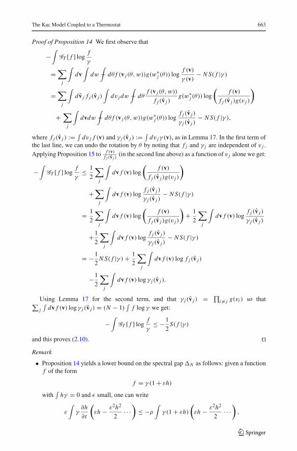
Proof of Proposition 14 We first observe that

−∫

GT [ f ] logf

γ

=∑

j

∫dv∫

dw∫− dθ f (v j (θ, w))g(w

∗j (θ)) log

f (v)γ (v)

− N S( f |γ )

=∑

j

∫d v̂ j f j (v̂ j )

∫dv j dw

∫− dθ

f (v j (θ, w))

f j (v̂ j )g(w∗

j (θ)) log

(f (v)

f j (v̂ j )g(v j )

)

+∑

j

∫dvdw

∫− dθ f (v j (θ, w))g(w

∗j (θ)) log

f j (v̂ j )

γ j (v̂ j )− N S( f |γ ),

where f j (v̂ j ) := ∫dv j f (v) and γ j (v̂ j ) := ∫

dv jγ (v), as in Lemma 17. In the first term ofthe last line, we can undo the rotation by θ by noting that f j and γ j are independent of v j .

Applying Proposition 15 to f (v)f j (v̂ j )

(in the second line above) as a function of v j alone we get:

−∫

GT [ f ] logf

γ≤ 1

2

∑

j

∫dv f (v) log

(f (v)

f j (v̂ j )g(v j )

)

+∑

j

∫dv f (v) log

f j (v̂ j )

γ j (v̂ j )− N S( f |γ )

= 1

2

∑

j

∫dv f (v) log

(f (v)

f j (v̂ j )g(v j )

)+ 1

2

∑

j

∫dv f (v) log

f j (v̂ j )

γ j (v̂ j )

+1

2

∑

j

∫dv f (v) log

f j (v̂ j )

γ j (v̂ j )− N S( f |γ )

= −1

2N S( f |γ )+ 1

2

∑

j

∫dv f (v) log f j (v̂ j )

−1

2

∑

j

∫dv f (v) log γ j (v̂ j ).

Using Lemma 17 for the second term, and that γ j (v̂ j ) = ∏i �= j g(vi ) so that∑

j

∫dv f (v) log γ j (v̂ j ) = (N − 1)

∫f log γ we get:

−∫

GT [ f ] logf

γ≤ −1

2S( f |γ )

and this proves (2.10). ��Remark

• Proposition 14 yields a lower bound on the spectral gapN as follows: given a functionf of the form

f = γ (1 + εh)

with∫

hγ = 0 and ε small, one can write

ε

∫γ∂h

∂t

(εh − ε2h2

2· · ·)

≤ −ρ∫γ (1 + εh)

(εh − ε2h2

2· · ·),

123


where ρ = μ/2. That is,∫γ h∂h

∂t≤ −ρ

∫γ h2

2.

Thus in L2(RN , γ (v)dv) we get

d

dt‖h‖ ≤ −ρ

2‖h‖.

Observe that this is very similar to the result one get from Proposition 1 but ρ < μ. Onemay wonder whether ρ is the optimal estimate for the decay rate of the relative entropy.

• In contrast to the Kac model, the presence of the thermostat guarantees that the rate ofconvergence is strictly positive uniformly in N . It is fundamental in the above analysisthat the thermostat acts on all particles. The presence of the Kac part gives no contributionto the above estimate of the exponential decay rate.

3 Propagation of Chaos

We finally turn our attention to the effective Boltzmann equation that emerges in the limitfor N → ∞. The fundamental step to this end is to show that the dynamics defined by Eq.(1.1) propagates chaos, which is done in this section.

Theorem 18 Let f (N )(v, 0) be a chaotic sequence of initial densities. Then its evolutionunder the master equation (1.1), f (N )(v, t), is a chaotic sequence for any fixed t. That is, if

limN→∞

∫

RN

ϕ1(v1) · · ·ϕk(vk) f (N )(v, 0) =k∏

j=1

limN→∞

∫

R

ϕ j (v j ) f (N )(v, 0)

for any k ∈ N and any φ1(v1), . . . φk(vk) bounded and continuous, then for any t:

limN→∞

∫

RN

ϕ1(v1) · · · ϕk(vk) f (N )(v, t) =k∏

j=1

limN→∞

∫

R

ϕ j (v j ) f (N )(v, t)

for any k ∈ N and any ϕ1(v1), . . . ϕk(vk) bounded and continuous.

The proof follows closely the McKean [2] algebraic version of Kac [1], for the Kacoperator. The idea is to write f (v, t) = e−(λGK +μGT )t f (v, 0), expand the exponential inseries of t , and use the chaotic property of the initial sequence. The key observation is thatGT is a derivation already for finite N (in the sense of Lemma 20). Two main ingredients areneeded:

Lemma 19 The series∑∞

l=0tl

l!∫ϕ1(v1) · · ·ϕk(vk)(λGK + μGT )

l f (v, 0) converges abs-

olutely if t < 14λ+μ .

Proof To prove the lemma, it is enough to show that:

||(λGK + μG ∗T )

lφ||∞ ≤ (4λ+ 2μ)lm(m + 1) · · · (m + l − 1)||φ||∞ (3.1)

and then follow the proof in [2]. The above statement follows from a simple induction startingfrom

123


|(λGK + μG ∗T )φ(v1, . . . , vm)| ≤ |λGKφ| + |μG ∗

T φ| ≤ (4λ+ 2μ)m||φ||∞.��

Calling

�Kφ := 2∑

i≤m

∫− dθ(φ(. . . , vi cos θ + vm+1 sin θ, . . .)− φ),

one can prove, as in [2], that if ϕ1(v1), . . . , ϕk(vk) are bounded and continuous then:

limN→∞

∫(λGK + μG ∗

T )l [ϕ1 · · · ϕk] f (N )(v, 0)= lim

N→∞

∫(λ�K +μG ∗

T )l [ϕ1 · · ·ϕk] f (N )(v, 0).

The main ingredient to re-sum the power series expansion and obtain the Boltzmannequation is the following “algebraic” Lemma.

Lemma 20 If (φ ⊗ ψ)(v1, . . . , vm+k) := φ(v1, . . . , vm)ψ(vm+1, . . . , vm+k), then

(�K + G ∗T )[φ ⊗ ψ] = (�K + G ∗

T )[φ] ⊗ ψ + φ ⊗ (�K + G ∗T )[ψ].

It is now possible to prove Theorem 5 by following the proof in [2] step-by-step.

4 Conclusion and Future Work

We hope to have convinced the reader that master equations of Kac type are reasonablemodels for large particle systems interacting with thermal reservoirs. The main advantage isthat physically relevant quantities such the first and second gap can be computed quite easilyand the entropic convergence to equilibrium can be established in a quantitative fashion aswell. Moreover, since propagation of chaos holds, contact is made with a Boltzmann typeequation in one dimension.

There are a number of directions for future research. The generalization to three-dimensional momentum-conserving collisions [21], while more complicated, should notpose any new real difficulties. There are other, more severe, assumptions made in our modelthat one ought to address.

For example, it is the very nature of a reservoir that it is not influenced by the interactionwith the other N particles. A more realistic situation would be to consider the reservoir asfinite but large. More precisely, consider an initial state of the form γ F where γ is a Gaussianin M variables with inverse temperatureβ and F a function of N variables with kinetic energyeN . Thus, M particles are in thermal equilibrium and N particles are not in equilibrium butwith finite energy per particle. Now we let this state evolve under the Kac evolution. Clearly,this state will evolve to a radial function in N + M variables as t → ∞. One would expectthat this function is close to a Gaussian with a temperature (M

β+ 2eN )/(M + N ). Assuming

that M >> N , is it true that the entropy has a rate of decay that is uniform in N? Notethat the problem is not to get an estimate on the entropy production of the initial state. Theinfinitesimal time evolution is precisely the weak thermostat treated in our paper. The realissue is to quantify the entropy production at later times for which the state is no longer ofthis simple form.

Another important issue is how to understand non-equilibrium steady states in a widersense. We believe that the Kac approach to kinetic theory could shed some light on this verydifficult problem. The fact that the particles interact with a single heat reservoir leads to anon-self-adjoint operator that can be brought into a self-adjoint form using a ground state

123


transformation. It is easy to write down the master equation for a system of particles thatinteract with, say, two reservoirs at different temperatures. However, the generator cannotbe brought into a self-adjoint form anymore and the equilibrium cannot be found thoughan optimization procedure, or at least not an obvious one. In particular the equilibrium isnot a simple function. How, then, can one measure the approach to steady-state for suchsystems? Note that the steady-state is, from the point of physics, not an equilibrium state,since it mediates an energy transport from a reservoir of higher temperature to one of lowertemperature. The solution of this problem would be a small step towards understandingnon-equilibrium steady states.

Acknowledgments The authors would like to thank Eric Carlen, Joel Lebowitz and Hagop Tossounianfor many enlightening discussions. We thank Hagop Tossounian for helping in the proof of Proposition 15.We also thank the referee for various helpful comments and the extremely detailed report. This work waspartially supported by U.S. National Science Foundation grant DMS 1301555. © 2013 by the authors. Thispaper may be reproduced, in its entirety, for non-commercial purposes.

References

1. Kac, M.: Foundations of kinetic theory. In: Proceedings of the Third Berkeley Symposium on Mathemat-ical Statistics and Probability. 1954–1955, vol. III, pp. 171–197. University of California Press, Berkeleyand Los Angeles (1956)

2. McKean Jr, H.P.: Speed of approach to equilibrium for kac’s caricature of a maxwellian gas. Arch. Ration.Mech. Anal. 21, 343–367 (1966)

3. Lanford III, O.E.: Time evolution of large classical systems. In: Dynamical Systems, Theory and Appli-cations (Recontres, Battelle Res. Inst., Seattle, Wash., 1974), pp. 1–111. Lecture Notes in Physics, vol.38. Springer, Berlin (1975)

4. Lanford III, O.E.: On a derivation of the Boltzmann equation. In: International Conference on DynamicalSystems in Mathematical Physics (Rennes, 1975), pp. 117–137. Astérisque, No. 40. Societe MathematiqueDe France, Paris (1976).

5. Illner, R., Pulvirenti, M.: Global validity of the Boltzmann equation for two- and three-dimensionalrare gas in vacuum. Erratum and improved result: “Global validity of the Boltzmann equation for atwo-dimensional rare gas in vacuum” [Comm. Math. Phys. 105(2), 1986, pp. 189–203; MR0849204(88d:82061)] and “Global validity of the Boltzmann equation for a three-dimensional rare gas in vacuum”[ibid. 113 (1987), no. 1, 79–85; MR0918406 (89b:82052)] by Pulvirenti. Comm. Math. Phys. 121(1),143–146 (1989). http://projecteuclid.org/getRecord?id=euclid.cmp/1104178007. Accessed 08 May 2014

6. Janvresse, E.: Spectral gap for Kac’s model of Boltzmann equation. Ann. Probab. 29(1), 288–304 (2001).doi:10.1214/aop/1008956330

7. Carlen, E., Carvalho, M.C., Loss, M.: Many-body aspects of approach to equilibrium. In: Journées “Équa-tions aux Dérivées Partielles” (La Chapelle sur Erdre, 2000), pp. Exp. No. XI, 12. University of Nantes,Nantes (2000)

8. Maslen, D.K.: The eigenvalues of Kac’s master equation. Math. Z. 243(2), 291–331 (2003). doi:10.1007/s00209-002-0466-y

9. Villani, C.: Cercignani’s conjecture is sometimes true and always almost true. Commun. Math. Phys.234(3), 455–490 (2003). doi:10.1007/s00220-002-0777-1

10. Einav, A.: On Villani’s conjecture concerning entropy production for the Kac master equation. Kinet.Relat. Models 4(2), 479–497 (2011). doi:10.3934/krm.2011.4.479

11. Fröhlich, J., Gang, Z.: Exponential convergence to the Maxwell distribution for some class of Boltzmannequations. Commun. Math. Phys. 314(2), 525–554 (2012). doi:10.1007/s00220-012-1499-7

12. Bonetto, F., Chernov, N., Korepanov, A., Lebowitz, J.L.: Nonequilibrium stationary state of a current-carrying thermostated system. EPL 102, 15001 (2013)

13. Bonetto, F., Carlen, E., Esposito, R., Lebowitz, J., Marra, R.: Propagation of chaos for a thermostatedkinetic model. http://arxiv.org/abs/1305.7282

14. Mischler, S., Mouhot, C.: Kac’s program in kinetic theory. Invent. Math. 193(1), 1–147 (2013). doi:10.1007/s00222-012-0422-3

15. Stam, A.J.: Some inequalities satisfied by the quantities of information of fisher and shannon. Inf. Control2, 101–112 (1959)

123

http://projecteuclid.org/getRecord?id=euclid.cmp/1104178007

http://dx.doi.org/10.1214/aop/1008956330

http://dx.doi.org/10.1007/s00209-002-0466-y

http://dx.doi.org/10.1007/s00209-002-0466-y

http://dx.doi.org/10.1007/s00220-002-0777-1

http://dx.doi.org/10.3934/krm.2011.4.479

http://dx.doi.org/10.1007/s00220-012-1499-7

http://arxiv.org/abs/1305.7282

http://dx.doi.org/10.1007/s00222-012-0422-3

http://dx.doi.org/10.1007/s00222-012-0422-3


16. Gross, L.: Logarithmic sobolev inequalities. Am. J. Math. 97(4), 1061–1083 (1975)17. Bakry, D., Émery, M.: Diffusions hypercontractives. In: Séminaire de Probabilités, XIX, 1983/84. Lecture

Notes in Mathematics, vol. 1123, pp. 177–206. Springer, Berlin (1985). doi:10.1007/BFb007584718. Gross, L.: Logarithmic Sobolev inequalities and contractivity properties of semigroups. In: Dirichlet

Forms (Varenna, 1992). Lecture Notes in Mathematics, vol. 1563, pp. 54–88. Springer, Berlin (1993).doi:10.1007/BFb0074091

19. Toscani, G.: Entropy production and the rate of convergence to equilibrium for the Fokker–Planck equa-tion. Quart. Appl. Math. 57(3), 521–541 (1999)

20. Loomis, L.H., Whitney, H.: An inequality related to the isoperimetric inequality. Bull. Am. Math. Soc55, 961–962 (1949)

21. Carlen, E.A., Geronimo, J.S., Loss, M.: Determination of the spectral gap in the Kac model for physicalmomentum and energy-conserving collisions. SIAM J. Math. Anal. 40(1), 327–364 (2008). doi:10.1137/070695423

123

http://dx.doi.org/10.1007/BFb0075847

http://dx.doi.org/10.1007/BFb0074091

http://dx.doi.org/10.1137/070695423

http://dx.doi.org/10.1137/070695423

the kac model coupled to a thermostat -...

Documents