J Geod (2011) 85:909–920DOI 10.1007/s00190-010-0427-x

REVIEW

The international reference ionosphere today and in the future

Dieter Bilitza · Lee-Anne McKinnell · Bodo Reinisch ·Tim Fuller-Rowell

Received: 10 June 2010 / Accepted: 16 November 2010© Springer-Verlag 2010

Abstract The international reference ionosphere (IRI) isthe internationally recognized and recommended standardfor the specification of plasma parameters in Earth’s ion-osphere. It describes monthly averages of electron density,electron temperature, ion temperature, ion composition, andseveral additional parameters in the altitude range from 60 to1,500 km. A joint working group of the Committee on SpaceResearch (COSPAR) and the International Union of RadioScience (URSI) is in charge of developing and improving theIRI model. As requested by COSPAR and URSI, IRI is anempirical model being based on most of the available andreliable data sources for the ionospheric plasma. The paperdescribes the latest version of the model and reviews effortstowards future improvements, including the development ofnew global models for the F2 peak density and height, and a

D. Bilitza (B)Space Weather Laboratory, George Mason University, Fairfax,VA 22030, USAe-mail: dbilitza@gmu.edu; dieter.bilitza-1@nasa.gov

D. BilitzaHeliospheric Laboratory, NASA Goddard Space Flight Center,Greenbelt, MD 20771, USA

L.-A. McKinnellHermanus Magnetic Observatory, PO Box 32,Hermanus 7200, South Africae-mail: lmckinnell@hmo.ac.za

B. ReinischCenter for Atmospheric Research, University of MassachusettsLowell, 600 Suffolk Street, Lowell, MA 01854, USAe-mail: Bodo_Reinisch@uml.edu

T. Fuller-RowellCIRES University of Colorado and NOAA Space Weather PredictionCenter, 325 Broadway, Boulder, CO 80305, USAe-mail: Tim.Fuller-Rowell@noaa.gov

new approach to describe the electron density in the topsideand plasmasphere. Our emphasis will be on the electron den-sity because it is the IRI parameter most relevant to geodetictechniques and studies. Annual IRI meetings are the mainvenue for the discussion of IRI activities, future improve-ments, and additions to the model. A new special IRI taskforce activity is focusing on the development of a real-timeIRI (RT-IRI) by combining data assimilation techniques withthe IRI model. A first RT-IRI task force meeting was held in2009 in Colorado Springs. We will review the outcome ofthis meeting and the plans for the future. The IRI homepageis at http://www.IRI.gsfc.nasa.gov.

Keywords Ionosphere · IRI · Empirical model ·F2 peak models · Topside

1 Introduction

Empirical models play an important role in all parts of theSun–Earth environment. They give the scientist, engineer,and educator easy access to a condensed form of the avail-able empirical evidence for a specific parameter, optimally,being based on all reliable data sources that exist for theparameter. Examples of such widely used models are theinternational geomagnetic reference field (IGRF) model forEarth’s magnetic field (IGRF 2010) and the Mass spectrom-eter and incoherent scatter (MSIS) model for Earth’s atmo-sphere (Picone et al. 2002). The ionospheric equivalent tothese models is the international reference ionosphere (IRI).Since initiated by the Committee on Space Research(COSPAR) and the International Union of Radio Science(URSI) in 1969, IRI has been steadily improved with newerdata and better modeling techniques leading to the release ofa number of key editions of the model including the IRI-78

123

910 D. Bilitza et al.

(Rawer et al. 1978), IRI-85 (Bilitza 1986), IRI-1990(Bilitza 1990), IRI-2000 (Bilitza 2001), and IRI-2007 (Bil-itza and Reinisch 2008). The model progressed from a setof tables of representative values to an analytical representa-tion of densities and temperatures on the whole globe. It is adata-based model, as requested by COSPAR and URSI, andwas developed making use of all available and reliable datasources for the ionospheric plasma. This includes the world-wide network of ionosondes that has monitored ionosphericelectron densities at and below the F-peak for more than halfa century, the powerful incoherent scatter radars that measureplasma densities, temperatures, and velocities throughout thewhole ionosphere, but unfortunately only at a few selectedlocations (∼8 in operation currently), the topside soundersatellites that have provided the global distribution of elec-tron density from the satellite altitude down to the F-peak, insitu satellite measurements of ionospheric parameters alongthe satellite orbit, and rocket observations of the lower ion-osphere, currently the only reliable method to obtain plasmaparameters in the D-region.

Being an empirical model IRI has the advantage that itdoes not depend on the evolving theoretical understandingof the processes that shape the ionospheric plasma. A goodexample is the recently discovered four maxima structurein the longitudinal variation of F-peak electron density andionospheric electron content that was first observed withIMAGE/EUV observations (Immel et al. 2006), and thenconfirmed with data from CHAMP (Lühr et al. 2007) andTOPEX (Schmidt et al. 2008) and that is thought to be causedby non-migrating, diurnal atmospheric tides that are, in turn,driven mainly by weather in the tropics. Although theoreticalmodels still grabble with including this phenomenon in theirmodeling framework, inspection of the longitudinal varia-tion of the F-peak density value NmF2 in IRI revealed thatIRI already reproduces this phenomenon (McNamara et al.2010). The amplitude of these longitudinal variations is gen-erally smaller in IRI than what is observed. However, that isunderstandable, because IRI is based on monthly averagesand the averaging process smoothes out some of these lon-gitude structures.

A disadvantage of empirical models is the strong depen-dence on the underlying data base. Regions and time periodsnot well covered by the data base will result in diminishedreliability of the model in these areas. So, for example, therepresentation of the F-peak density (NmF2; see Sect. 4) inIRI is based on the data from the global network of ionoson-des. The model performs best at continental northern mid-latitudes because that is the region with the highest densityof ionosondes stations and many of these stations have beenoperating over a long time period. Most difficult are the oceanareas, where only a few island stations exist and an interpola-tion scheme has to be applied to cover this part of the globe.The two major models in use for NmF2, the CCIR (1966)

and URSI-88 (Rush et al. 1989), differ primarily in the inter-polation scheme used for the ocean areas. IRI offers use ofboth models and based on the data background recommendsthe CCIR model for the continents and the URSI-88 modelfor the ocean areas. A radically new modeling approach forthis important parameter will be described in Sect. 4 of thispaper.

The main venue for improvements of the IRI model areannual workshops during which the latest results are pre-sented and discussed and decisions are made regarding modelupdates and additions. A new effort was started in 2009 thathas as its goal the development of the real-time IRI (RT-IRI).A first RT-IRI meeting was held at the US Air Force Acad-emy in Colorado Springs, Colorado, USA in May 2009. Theresults from the meeting and plans for the future regardingthis activity will be discussed in Sect. 6.

2 IRI relevance to geodetic techniques

From the start applications of the model have been an impor-tant driver for the IRI development and improvement activi-ties. IRI applications range across a wide user community andthis importance was recognized by the InternationalStandardization Organization (ISO) by voting it the recom-mended technical specification for ionospheric parameters(ISO 2009). Here, we will focus on applications of IRI inthe realm of geodetic techniques. We will also discuss thepotential impact of ionospheric data deduced from geodetictechniques towards improvements of IRI.

One important role of IRI is as a background ionospherefor validating the reliability and accuracy of a particularapproach for deducing ionospheric parameters from geodeticmeasurements. Hernandez-Pajares et al. (2002) and Niran-jan et al. (2007) have used IRI for testing algorithms thatconvert GPS measurements into global total electron con-tent (TEC) maps. Many tomographic techniques and radiooccultation inversion algorithms got their real first test in anIRI background ionosphere (Bust et al. 2004; Lee et al. 2008;Garcia and Crespon 2008). Starting out with an IRI groundtruth ionosphere, the simulated geodetic measurements arecomputed for this ionosphere and than the tomographic algo-rithm is applied to reconstruct the underlying ionosphere,which is then compared against the original IRI ground truth.Hocke and Igarashi (2002) used the same approach to validatetheir GPS/MET occultation measurement algorithm and Dearand Mitchell (2006) for testing their MIDAS GPS technique.Most of these techniques rely on an iterative mathemati-cal process and many use IRI to define the initial condi-tions for this process (e.g., Bust et al. 2004). Another areawhere IRI has helped these techniques is with interpolat-ing in regions where no GPS measurements are available(e.g.,Orús et al. 2002). Interesting also is the work of

123

The international reference ionosphere today and in the future 911

Datta-Barua et al. (2008), who estimated the range ofhigh-order ionospheric errors for the dual-frequency GPSuser based on an IRI ionosphere.

Global TEC maps represent the vertical TEC while GPSmeasurements provide the slant TEC along the path fromground station to satellite. Conversion from slant TEC tovertical TEC is in most cases performed using a thin shellapproach which assumes that the ionospheric plasma is com-pressed into a thin shell at height hts. The conversion factordepends on the elevation angle of the slant path and on hts.Many techniques still use a constant (often 300 km) height hts

for this conversion, even though it has been shown that usingthe varying height of maximum density from IRI, hmF2 pro-duces superior results (Komjathy et al. 1998; Brunini et al.2003).

Ionospheric parameters deduced from geodetic measure-ments are an excellent resource for improving the IRI model.Of greatest interest are electron density profiles deducedthrough tomography and occultation. Validation of thesetechniques is progressing successfully, but a few open ques-tions still remain regarding inherent limitation of these tech-niques in regions of steep gradients and areas of sparse groundstation coverage (e.g., the ocean areas). Integral measure-ments (TEC), on the other hand, are widely used for spaceweather applications and only a few small issues remain hav-ing to do with the inherent instrument bias (Garner et al. 2008)and the conversion algorithm as noted earlier in this section.Bias uncertainties remain also for vertical TEC measure-ments from dual altimeter instruments like TOPEX, Jasonand ERS. Altimeter data complement the GPS data becausethey provide TEC over the oceans, but not over land. Theyare an excellent data source for model validations, especiallyin relation to the relative variation of model parameters thusavoiding bias uncertainties.

Komjathy et al. (1998) were one of the first to assimilateglobal TEC maps deduced from GPS measurements into theIRI model and thus updating the monthly average model tothe daily and hourly ionospheric conditions monitored byGPS. An even more direct approach by Hernandez-Pajareset al. (2002) made use of individual slant TEC measure-ments. They determine an equivalent solar index by adjustingIRI-slant-TEC to the measured slant-TEC and than use IRIwith this modified solar index. More recently, Schmidt et al.(2008) and Zeilhofer et al. (2009) have developed a 4-D rep-resentation of the ionospheric electron density using IRI asreference model and using an expansion in B-spline functionsto describe the difference term between the reference modeland the data (see article by Dettmering et al. in this issue).Other IRI-GPS assimilation schemes have been developedby Fuller-Rowell et al. (2006) using IRI deduced EOF func-tions to represent TEC over the continental USA (US-TEC)and by Angling et al. (2009) using IRI and GPS data in theirelectron density assimilative model (EDAM).

3 Status and plans

The newest version of the IRI model, IRI-2011, will includesignificant improvements not only for the representations ofelectron density, but also for the description of electron tem-perature and ion composition. These improvements are theresult of modeling efforts, since the last major release, IRI-2007. Modeling progress is documented in several specialissues of Advances in Space Research: Volume 39, Number 5,2007; Volume 42, Number 4, Aug 2008; Volume 43, Number11, June 2009; Volume 44, Number 6, September 2009.

Our focus here will be only on those improvements thatwill have an impact on the electron density which is theparameter of most interest for geodetic techniques and dataanalysis. One of the most important changes is the inclusionof new neural network-based models for the point of highestdensity which are explained in Sect. 4.

In the bottomside the IRI electron density profile is nor-malized to the E and F2 peaks and the shape of the profileis determined by the bottomside thickness parameter B0 andthe shape parameter B1. Currently, two options are givenfor these parameters: (i) the standard option consisting ofa table of values and associated interpolation scheme (Bil-itza et al. 2000) and (ii) the Gulyaeva option based on themodel of Gulyaeva (1987) utilizing the half-density pointh0.5 where the topside density has dropped down to half thepeak density. Shortcomings of these older models are theirlimited data base and the resulting misrepresentation of vari-ations with season, latitude and solar activity. Altadill et al.(2008, 2009) have applied spherical harmonic analysis to datafrom 27 globally distributed ionosondes stations obtaining anew model for B0 and B1 that more accurately describes theobserved variations with latitude, local time, month, and sun-spot number. Overall, the improvements over the older IRImodel are of the order of 15–35%. The largest improvementsare seen at low latitudes.

At high-latitudes the off-set of the magnetic pole fromthe geographic pole and its rotation around the geographic(rotation axis) pole together with the influx of energetic solarwind particles results in the formation of the auroral oval atthe boundary between closed and open magnetic field lines.Ionospheric densities and temperatures exhibit characteristicvariations in and near the oval region and, therefore, the inclu-sion of an oval description in IRI has long been a high priorityof the IRI team (e.g., Szuszczewicz et al. 1993 and Bilitza1995) and is the first step towards including high-latitudecharacteristics in IRI. Zhang and Paxton (2008) have recentlydeveloped a model of the auroral electron energy flux basedon the global far ultraviolet (FUV) measurements with theglobal ultraviolet imager (GUVI) on the thermosphere iono-sphere mesosphere energetics and dynamics (TIMED) satel-lite. The model also describes the expansion of the ovalduring magnetic storms. Using a threshold flux value

123

912 D. Bilitza et al.

Zhang et al. (2010) define the poleward and equatorwardboundaries of the oval and their movement with magneticactivity. This boundary parameterization is now scheduledfor inclusion in IRI.

During night time infrared emissions measured by anotherTIMED instrument, the sounding of the atmosphere usingbroadband emission radiometry (SABER) instrument, willhelp us to represent in IRI the storm induced enhancementsof the E-region electron density that is caused by increasedparticle precipitation. Mertens et al. (2007) and Fernandezet al. (2010) have developed a model for the E-peak enhance-ment for different levels of magnetic activity using a formal-ism similar to the one used in the F-region STROM modelof Fuller-Rowell et al. (2000). Comparisons with incoherentscatter radar measurements show good agreement (Fernandezet al. 2010).

In addition, IRI-2010 will make use of the latest version ofthe International Geomagnetic Reference Field (IGRF 2010)for its computation of magnetic coordinates.

These changes will result in significant improvements ofIRI electron densities and total electron content (TEC) and,therefore, will benefit the many applications of the IRI modelfor geodetic techniques and data analysis.

4 New global models for the F2 peak parameters

The point of highest density in the ionosphere, the F2 peak,is defined by two parameters the peak height (hmF2) and thepeak plasma frequency (foF2) which is directly related to thesquare-root of the F2 peak density. A third parameter alsoof interest here is the propagation factor M(3000)F2, whichcan be monitored from the ground with the help of ionoson-des and which is inversely related to hmF2. Currently, newneural network (NN) based global models for the F2 peakparameters (foF2 and M(3000)F2) are being developed andevaluated as a possible replacement for the CCIR (1966) andURSI (Rush et al. 1989) models presently used as IRI F2 peakparameter prediction tools. The NN is the technique, wherebya computer is trained to learn the relationship between a givenset of inputs and a known output. This technique is very use-ful in predicting non-linear relationships, and makes use ofthe history of what has come before. Therefore, it is crucial tohave a large database of archived data from which to developthe NN based model. The NNs used in this work make use ofthe feed forward back propagation algorithm and the readeris referred to Haykin (1994) for more details on the workingof NNs.

4.1 foF2 model

Initially, a global foF2 model was developed using hourlyvalues of foF2 from 85 global ionospheric stations, spanningthe period 1995–2005 and for a few stations from 1976 to

1986. Data from various resources of the World Data Centre(WDC) archives (Space Physics Interactive Data ResourceSPIDR, the Digital Ionogram Database, DIDBase, and IPSRadio and Space Services) have been used in the develop-ment of the model. To satisfy all requirements for the model,data from all latitude regions with different levels of magneticand solar activity and season were used to test for the predic-tive ability of the NN model and the results were comparedwith the URSI and CCIR predictions of the IRI model. Asshown in Oyeyemi and McKinnell (2008), a large percentageof the data used is from the northern hemisphere, while fewof the data are from the southern hemisphere with not mucharound the equatorial region. A significant paucity of datafrom the polar sectors (north and south) was also found. Thedatabase consisted of a mixture of manually edited and auto-matically scaled data. Because it was too man-hour intensiveto manually edit all of the data, a general trend analysis wasperformed on all of the data to ensure that there were noextreme outliers and obvious defects in the scaling. The NNtechnique is able to cope with minor problems in the datain that the technique aims for the best average solution, andwill ignore a few serious outliers. The final NN input spacefor the first version of the foF2 global model consisted ofday number, universal time, solar zenith angle, solar activity,magnetic activity, day-of-year, geographic latitude, magneticinclination and declination. For detailed information on theinputs to the NN the reader is referred to Oyeyemi (2005)and Oyeyemi et al. (2005).

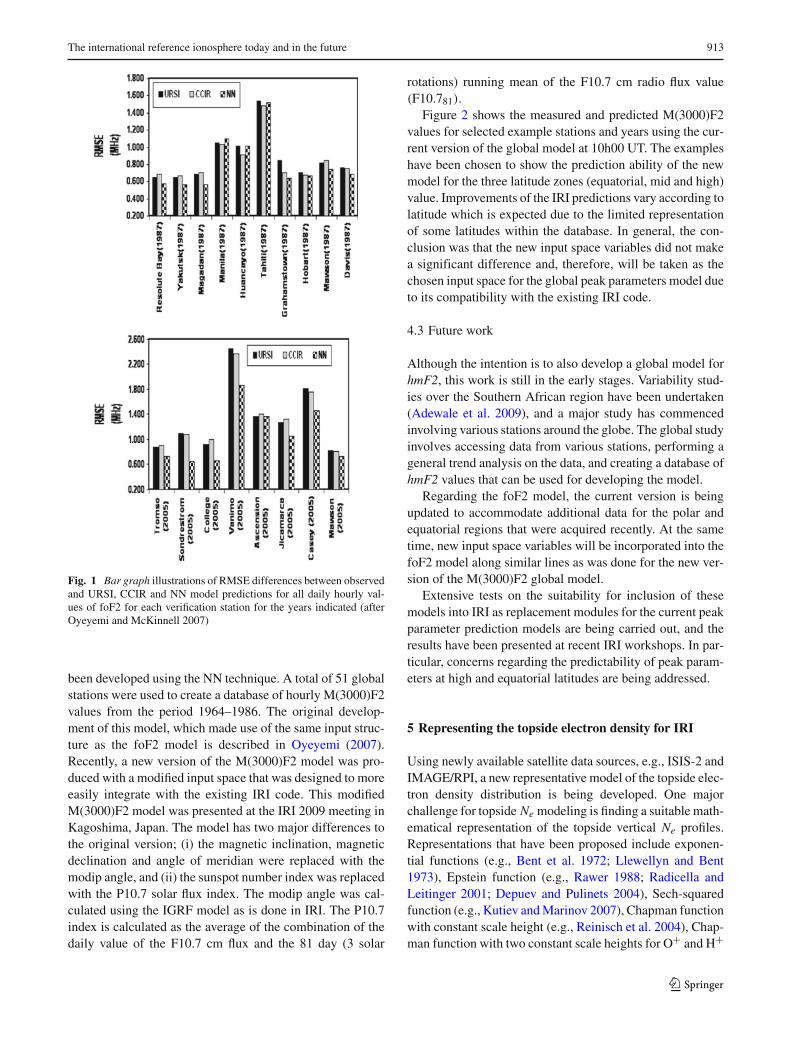
The NN model for predicting the global foF2 value hasbeen tested extensively to judge its ability to meet the require-ments for the replacement of the IRI foF2 maps. Figure 1shows the bar graphs illustrating the RMSE differencesbetween observed foF2 values and predictions by the NNmodel and the IRI model (URSI and CCIR coefficients) forthe foF2 hourly values for a few stations. Further discus-sion on the testing procedure can be found in McKinnell andOyeyemi (2009).

Currently, work is progressing on the development andevaluation of this model. Additional data have been acquiredto address the gaps in the distribution, particularly at thepolar and equatorial regions, and this data will be added tothe database and the NN re-trained. The input space is alsobeing assessed since the current input space is not compatiblewith the current IRI code, and a more compatible input spaceis required. At each stage of the development, the model istested and compared with IRI to ensure that the replacementsolution for the foF2 maps predicts to a greater accuracy thanthe current IRI solution.

4.2 M(3000)F2 model

Similarly to the above-described method for developing anew foF2 model, a model for the M(3000)F2 parameter has

123

The international reference ionosphere today and in the future 913

Fig. 1 Bar graph illustrations of RMSE differences between observedand URSI, CCIR and NN model predictions for all daily hourly val-ues of foF2 for each verification station for the years indicated (afterOyeyemi and McKinnell 2007)

been developed using the NN technique. A total of 51 globalstations were used to create a database of hourly M(3000)F2values from the period 1964–1986. The original develop-ment of this model, which made use of the same input struc-ture as the foF2 model is described in Oyeyemi (2007).Recently, a new version of the M(3000)F2 model was pro-duced with a modified input space that was designed to moreeasily integrate with the existing IRI code. This modifiedM(3000)F2 model was presented at the IRI 2009 meeting inKagoshima, Japan. The model has two major differences tothe original version; (i) the magnetic inclination, magneticdeclination and angle of meridian were replaced with themodip angle, and (ii) the sunspot number index was replacedwith the P10.7 solar flux index. The modip angle was cal-culated using the IGRF model as is done in IRI. The P10.7index is calculated as the average of the combination of thedaily value of the F10.7 cm flux and the 81 day (3 solar

rotations) running mean of the F10.7 cm radio flux value(F10.781).

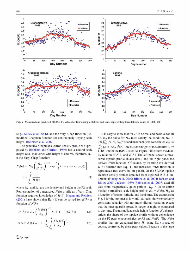
Figure 2 shows the measured and predicted M(3000)F2values for selected example stations and years using the cur-rent version of the global model at 10h00 UT. The exampleshave been chosen to show the prediction ability of the newmodel for the three latitude zones (equatorial, mid and high)value. Improvements of the IRI predictions vary according tolatitude which is expected due to the limited representationof some latitudes within the database. In general, the con-clusion was that the new input space variables did not makea significant difference and, therefore, will be taken as thechosen input space for the global peak parameters model dueto its compatibility with the existing IRI code.

4.3 Future work

Although the intention is to also develop a global model forhmF2, this work is still in the early stages. Variability stud-ies over the Southern African region have been undertaken(Adewale et al. 2009), and a major study has commencedinvolving various stations around the globe. The global studyinvolves accessing data from various stations, performing ageneral trend analysis on the data, and creating a database ofhmF2 values that can be used for developing the model.

Regarding the foF2 model, the current version is beingupdated to accommodate additional data for the polar andequatorial regions that were acquired recently. At the sametime, new input space variables will be incorporated into thefoF2 model along similar lines as was done for the new ver-sion of the M(3000)F2 global model.

Extensive tests on the suitability for inclusion of thesemodels into IRI as replacement modules for the current peakparameter prediction models are being carried out, and theresults have been presented at recent IRI workshops. In par-ticular, concerns regarding the predictability of peak param-eters at high and equatorial latitudes are being addressed.

5 Representing the topside electron density for IRI

Using newly available satellite data sources, e.g., ISIS-2 andIMAGE/RPI, a new representative model of the topside elec-tron density distribution is being developed. One majorchallenge for topside Ne modeling is finding a suitable math-ematical representation of the topside vertical Ne profiles.Representations that have been proposed include exponen-tial functions (e.g., Bent et al. 1972; Llewellyn and Bent1973), Epstein function (e.g., Rawer 1988; Radicella andLeitinger 2001; Depuev and Pulinets 2004), Sech-squaredfunction (e.g., Kutiev and Marinov 2007), Chapman functionwith constant scale height (e.g., Reinisch et al. 2004), Chap-man function with two constant scale heights for O+ and H+

123

914 D. Bilitza et al.

M30

00F

2

2

2.2

2.4

2.6

2.8

3

3.2

3.4

3.6

3.8

4

0 50 100 150 200 250 300 350

Day Number

Measured

Predicted

Grahamstown 1988

2

2.2

2.4

2.6

2.8

3

3.2

3.4

3.6

3.8

4

0 50 100 150 200 250 300 350

Day Number

M30

00F

2

Measured

Predicted

Grahamstown 1992

2

2.2

2.4

2.6

2.8

3

3.2

3.4

3.6

3.8

4

0 50 100 150 200 250 300 350

Day Number

M30

00F

2

Measured

Predicted

Argentine Islands 1987

2

2.2

2.4

2.6

2.8

3

3.2

3.4

3.6

3.8

4

0 50 100 150 200 250 300 350

Day Number

Measured

Predicted

Vanimo 1987

M30

00F

2

Fig. 2 Measured and predicted M(3000)F2 values for four example stations and years representing three latitude zones at 10h00 UT

(e.g., Kutiev et al. 2006), and the Vary–Chap function (i.e.,modified Chapman function for continuously varying scaleheight) (Reinisch et al. 2007).

The general α-Chapman electron density profile N(h) pro-posed by Rishbeth and Garriott (1969) has a neutral scaleheight H(h) that varies with height h, and we, therefore, callit the Vary–Chap function:

Ne(h) = Nm

(Hm

H (h)

)1/2

exp

[1

2(1 − y − exp (−y))

],

y =h∫

hm

dz

H (z)(1)

where Nm and hm are the density and height at the F2 peak.Representation of a measured N (h) profile as a Vary–Chapfunction requires knowledge of H (h). Huang and Reinisch(2001) have shown that Eq. (1) can be solved for H (h) asfunction of N (h)

H (h) = Hm

(N (h)

Nm

)−2

X (h) [1 − lnX (h)] (2a)

where X (h) = 1 + 1

Hm

h∫hm

(N (z)

Nm

)2

dz (2b)

It is easy to show that for H to be real and positive for allh > hm the value for Hm must satisfy the condition Hm ≥0.6

∫ hshm

[N (z)/Nm]2dz and in our analysis we selected Hm =∫ hshm

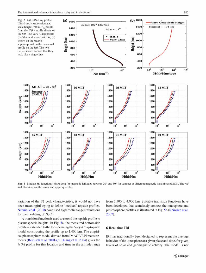
[N (z)/Nm]2dz. Here hs is the height of the satellite; hs ≈1,400 km for the ISIS-2 satellite. Figure 3 illustrates the dual-ity relation of N(h) and H (h). The left panel shows a mea-sured topside profile (black dots), and the right panel thederived H (h) function. Of course, by inserting this derivedH (h) function into Eq. (1), the measured N (h) function isreproduced (red curve in left panel). Of the 80,000 topsideelectron density profiles obtained from digitized ISIS-2 ion-ograms (Huang et al. 2002; Bilitza et al. 2004; Benson andBilitza 2009; Jackson 1969). Reinisch et al. (2007) used alldata from magnetically quiet periods (Kp ≤ 3) to derivemedian normalized scale height profiles Hn = H(h)/Hm asa function of season, latitude, and local time. The examples inFig. 4 for the summer at low mid-latitudes show remarkablyconsistent behavior with not much diurnal variation exceptthat the inter-quartile spread is larger at night as comparedto daytime. The normalized scale height function Hn charac-terizes the shape of the topside profile without dependenceon the F2 peak characteristics hmF2 and NmF2. The N (h)profiles that are calculated from Hn using Eq. (1) are, ofcourse, controlled by these peak values. Because of the large

123

The international reference ionosphere today and in the future 915

Fig. 3 left ISIS-2 Ne profile(black dots), right calculatedscale height H(h)/Hm profilefrom the N (h) profile shown onthe left. The Vary–Chap profile(red line) calculated with Hn(h)

shown on the right issuperimposed on the measuredprofile on the left. The twocurves match so well that theylook like a single line

Fig. 4 Median Hn functions (black line) for magnetic latitudes between 20◦ and 30◦ for summer at different magnetic local times (MLT). The redand blue dots are the lower and upper quartiles

variation of the F2 peak characteristics, it would not havebeen meaningful trying to define “median” topside profiles.Nsumei et al. (2010) have used hyperbolic tangent functionsfor the modeling of Hn(h).

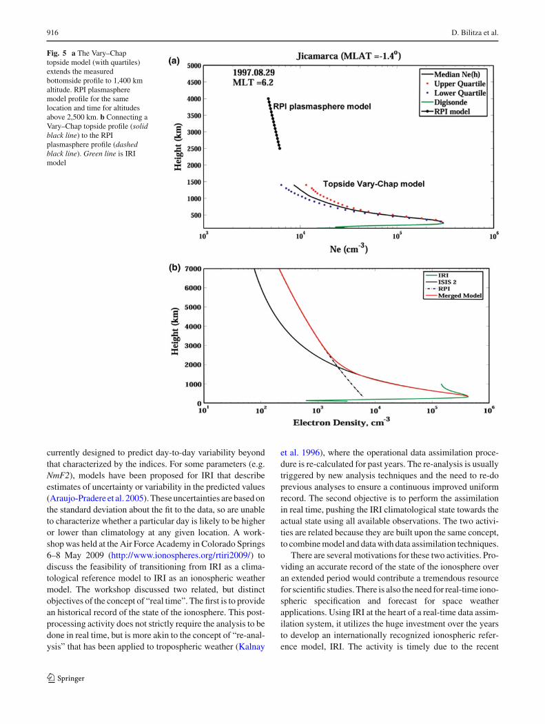
A transition function is used to extend the topside profile toplasmaspheric heights. In Fig. 5a, the measured bottomsideprofile is extended to the topside using the Vary–Chap topsidemodel constructing the profile up to 1,400 km. The empiri-cal plasmasphere model derived from IMAGE/RPI measure-ments (Reinisch et al. 2001a,b; Huang et al. 2004) gives theN (h) profile for this location and time in the altitude range

from 2,500 to 4,000 km. Suitable transition functions havebeen developed that seamlessly connect the ionosphere andplasmasphere profiles as illustrated in Fig. 5b (Reinisch et al.2007).

6 Real-time IRI

IRI has traditionally been designed to represent the averagebehavior of the ionosphere at a given place and time, for givenlevels of solar and geomagnetic activity. The model is not

123

916 D. Bilitza et al.

Fig. 5 a The Vary–Chaptopside model (with quartiles)extends the measuredbottomside profile to 1,400 kmaltitude. RPI plasmaspheremodel profile for the samelocation and time for altitudesabove 2,500 km. b Connecting aVary–Chap topside profile (solidblack line) to the RPIplasmasphere profile (dashedblack line). Green line is IRImodel

currently designed to predict day-to-day variability beyondthat characterized by the indices. For some parameters (e.g.NmF2), models have been proposed for IRI that describeestimates of uncertainty or variability in the predicted values(Araujo-Pradere et al. 2005). These uncertainties are based onthe standard deviation about the fit to the data, so are unableto characterize whether a particular day is likely to be higheror lower than climatology at any given location. A work-shop was held at the Air Force Academy in Colorado Springs6–8 May 2009 (http://www.ionospheres.org/rtiri2009/) todiscuss the feasibility of transitioning from IRI as a clima-tological reference model to IRI as an ionospheric weathermodel. The workshop discussed two related, but distinctobjectives of the concept of “real time”. The first is to providean historical record of the state of the ionosphere. This post-processing activity does not strictly require the analysis to bedone in real time, but is more akin to the concept of “re-anal-ysis” that has been applied to tropospheric weather (Kalnay

et al. 1996), where the operational data assimilation proce-dure is re-calculated for past years. The re-analysis is usuallytriggered by new analysis techniques and the need to re-doprevious analyses to ensure a continuous improved uniformrecord. The second objective is to perform the assimilationin real time, pushing the IRI climatological state towards theactual state using all available observations. The two activi-ties are related because they are built upon the same concept,to combine model and data with data assimilation techniques.

There are several motivations for these two activities. Pro-viding an accurate record of the state of the ionosphere overan extended period would contribute a tremendous resourcefor scientific studies. There is also the need for real-time iono-spheric specification and forecast for space weatherapplications. Using IRI at the heart of a real-time data assim-ilation system, it utilizes the huge investment over the yearsto develop an internationally recognized ionospheric refer-ence model, IRI. The activity is timely due to the recent

123

The international reference ionosphere today and in the future 917

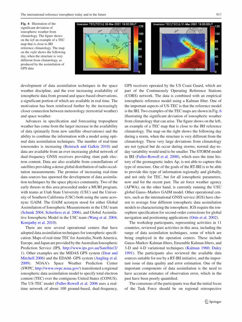
Fig. 6 Illustration of thesignificant deviation ofionospheric weather fromclimatology. The figure showson the left an example of a TECmap that is close to IRIreference climatology. The mapon the right shows the followingday, when the structure is verydifferent from climatology, asproduced by the assimilation ofGPS data

development of data assimilation techniques in the spaceweather discipline, and the ever increasing availability ofionospheric data from ground and space-based observations,a significant portion of which are available in real time. Themotivation has been reinforced further by the increasinglycloser connection between meteorology (terrestrial weather)and space weather.

Advances in specification and forecasting troposphereweather has come from the larger increase in the availabilityof data (primarily from new satellite observations) and theability to combine the information with a model using opti-mal data assimilation techniques. The number of real-timeionosondes is increasing (Reinisch and Galkin 2010) anddata are available from an ever-increasing global network ofdual-frequency GNSS receivers providing slant path elec-tron content. Data are also available from constellations ofsatellites providing a dense global distribution of radio occul-tation measurements. The promise of increasing real-timedata sources has spawned the development of data assimila-tion techniques by the space physics community. Two of theearly thrusts in this area proceeded under a MURI program,with teams at Utah State University (USU) and the Univer-sity of Southern California (USC) both using the same acro-nym: GAIM. The GAIM acronym stood for either GlobalAssimilation of Ionospheric Measurements in the USU team(Schunk 2004; Scherliess et al. 2006), and Global Assimila-tive Ionospheric Model in the USC team (Wang et al. 2004;Komjathy et al. 2010).

There are now several operational centers that haveadopted data assimilation techniques for ionospheric specifi-cation. Maps of real-time TEC for Australia, North America,Europe, and Japan are provided by the Australian IonosphericPrediction Service (IPS, http://www.ips.gov.au/Satellite/2/1). Other examples are the MIDAS GPS system (Dear andMitchell 2006) and the EDAM- GPS system (Angling et al.2009). NOAA’s Space Weather Prediction Center(SWPC, http://www.swpc.noaa.gov/) transitioned a regionalionospheric data assimilation model to specify total electroncontent (TEC) over the contiguous United States (CONUS).The US-TEC model (Fuller-Rowell et al. 2006 uses a real-time network of about 100 ground-based, dual-frequency,

GPS receivers operated by the US Coast Guard, which arepart of the Continuously Operating Reference Stations(CORS) network. The data is combined with an empiricalionospheric reference model using a Kalman filter. One ofthe important aspects of US-TEC is that the reference modelis the IRI. Two examples of the TEC maps are shown in Fig. 6illustrating the significant deviation of ionospheric weatherfrom climatology that can arise. The figure shows on the left,an example of a TEC map that is close to the IRI referenceclimatology. The map on the right shows the following dayduring a storm, when the structure is very different from theclimatology. These very large deviations from climatologyare not typical but do occur during storms; normal day-to-day variability would tend to be smaller. The STORM modelin IRI (Fuller-Rowell et al. 2000), which uses the time his-tory of the geomagnetic index Ap, is not able to capture thistype of structure. One of the goals of the RT-IRI is to be ableto provide this type of information regionally and globally,and not only for TEC, but for all ionospheric parameters,now and for the recent past. The air force weather agency(AFWA), on the other hand, is currently running the USUglobal Gauss–Markov GAIM model. Other operational cen-ters, such as the international GNSS service (IGS) have cho-sen to average four different ionospheric data assimilationmodels to characterizing the ionosphere. IGS require the ion-osphere specification for second-order corrections for globalnavigation and positioning applications (Orús et al. 2002).

The workshop participants, representing activities in 11countries, reviewed past activities in this area, including therange of data assimilation techniques, some of which arebeing employed in the operation centers. These includeGauss-Markov Kalman filters, Ensemble Kalman filters, and3-D and 4-D variational techniques (Kalman 1960; Daley1991). The participants also reviewed the available datasources suitable for use by a RT-IRI initiative, and the impor-tant issue of data quality and error estimation. One of theimportant components of data assimilation is the need tohave accurate estimates of observation error, which in thepast have been poorly quantified.

The consensus of the participants was that the initial focusof the Task Force should be on regional retrospective

123

918 D. Bilitza et al.

analysis for selected periods, and eventually combine theregions to produce a global specification in real time. Theparameters chosen to target were the 2-D maps of NmF2,hmF2, and TEC, plus estimates of uncertainty, graduallymigrating to the 3D ionospheric structure later. The data cho-sen for this first study would include hand-scaled ionogramsand ground-based GNSS receivers. Just as in troposphericnumerical weather prediction (NWP), new datasets will beadded after careful evaluation of their impact on the analy-sis (Cucurull et al. 2006). This will include radio occultationdata from the COSMIC satellite constellation (Anthes et al.2008). In the future, the assimilation period will be extendedand the results made available to the community on the IRIweb page for scientific studies. The group will also exploremethodologies to combine the regional maps to produce aglobal high-resolution analysis, recognizing the limitationsin the accuracy in data sparse regions. The availability ofspace based radio occultation data will be particularly impor-tant to improve the accuracy over the oceans.

7 Conclusions

We have presented the current status of IRI modeling activ-ities and plans for the future with special emphasis on theparameters and regions that are most important for geodeticmeasurement techniques and their data analysis schemes. IRIand geodetic techniques have benefitted each other. We havepresented many examples of applications of IRI in geodetictechniques. This includes the use of the height of largestdensity from IRI for the conversion of slant GPS-TEC tovertical TEC. IRI has been widely used as a backgroundmodel to test tomographic and radio occultation algorithmsrelated to signals from high and low orbiting GPS satellites.In turn ionospheric measurements from geodetic techniquesare a promising new resource for improvements of IRI and anexcellent candidate for data assimilation into the IRI model.With data assimilation the IRI model can progress from themonthly average conditions (climatology) that it is represent-ing now to daily and hourly conditions if a good set of globalobservations is available. The ultimate goal is the develop-ment of a Real Time IRI that assimilates all available andreliable ionospheric measurements into the model includingionosonde and incoherent scatter radar measurements frombelow, satellite in situ measurements from within, and GPSand radio occultation measurements from above. The IRIcommunity is ideally suited to perform this new extension tothe capabilities of this internationally recognized ionosphericreference model. The IRI science community has a long his-tory of working together efficiently and productively. Withthe increase in the number of data sources and the develop-ment of data assimilation techniques in the ionospheric com-munity this is the right time to make this important advance,

and follow the lead from the tropospheric weather forecastingcommunity.

Acknowledgments We acknowledge the contributions of IRI Work-ing Group members to the IRI effort and the many users of the modelwho have provided valuable feedback. This work was supported throughNSF grant ATM-0819440 and NASA Grants NNX09AJ74G, NNX07-AG38G, and NNX07AO65G.

References

Adewale AO, Oyeyemi EO, McKinnell LA (2009) Comparisons ofobserved ionospheric F2 peak parameters with IRI-2001 predic-tions over South Africa. J Atmos Solar Terr Phys 71(2):273–284.doi:10.1016/j.jastp.2008.10.014

Altadill D, Arrazola D, Blanch E, Buresova D (2008) Solar activityvariations of ionosonde measurements and modeling results. AdvSpace Res 42:610–616. doi:10.1016/j.asr.2007.07.028

Altadill D, Torta JM, Blanch E (2009) Proposal of new models ofthe bottom-side B0 and B1 parameters for IRI. Adv Space Res43:1825–1834. doi:10.1016/j.asr.2008.08.0144

Angling M, Shaw J, Shukla A, Cannon P (2009) Development of an HFselection tool based on the Electron Density Assimilative Modelnear-real-time ionosphere. Radio Sci 44:RS0A13. doi:10.1029/2008RS004022

Anthes RA, Ector D, Hunt DC, Kuo Y-H, Rocken C, Schreiner WS,Sokolovskiy SV, Syndergaard S, Wee T-K, Zeng Z, BernhardtPA, Dymond KF, Chen Y, Liu H, Manning K, Randel WJ,Trenberth KE, Cucurull L, Healy SB, Ho S-P, McCormick C,Meehan TK, Thompson DC (2008) The COSMIC/FORMOSAT-3mission: early results. Bull Am Meteorol Soc 89:313–333. doi:10.1175/BAMS-89-3-313

Araujo-Pradere EA, Fuller-Rowell TJ, Codrescu MV, Bilitza D(2005) Characteristics of the ionospheric variability as a functionof season, latitude, local time, and geomagnetic activity. Radio Sci40:RS 5009. doi:10.1029/2004RS003179

Araujo-Pradere EA, Fuller-Rowell TJ, Spencer PSJ, Minter CF(2007) Differential validation of the US-TEC model. Radio Sci42:RS3016. doi:10.1029/2006RS003459

Benson RF, Bilitza D (2009) New satellite mission with old data: res-cuing a unique data set. Radio Sci 44:RS0A04. doi:10.1029/2008RS004036

Bent RB, Llewellyn SK, Schmid PE (1972) Description and evalua-tion of the Bent ionospheric model, vol 1–3. National InformationService, Springfield, Virginia AD-753-081,-082,-083

Bilitza D (1986) International reference ionosphere: recent develop-ments. Radio Sci 21:343–346

Bilitza D (1990) International reference ionosphere 1990, NSSDC/WDC-A-R&S 90-22. National Space Science Data Center, Green-belt

Bilitza D (1995) Including auroral boundaries in the IRI model. AdvSpace Res 16(1):13–16

Bilitza D, Radicella S, Reinisch B, Adeniyi J, Mosert M, Zhang S,Obrou O (2000) New B0 and B1 models for IRI. Adv Space Res25(1):89–95

Bilitza D (2001) International reference ionosphere 2000. Radio Sci36(2):261–275

Bilitza D, Huang X, Reinisch B, Benson R, Hills HK, Schar WB(2004) Topside ionogram scaler with true height algorithm (TO-PIST): automated processing of ISIS topside ionograms. Radio Sci39(1):RS1S27. doi:10.1029/2002RS002840

Bilitza D, Reinisch BW (2008) International reference ionosphere2007: improvements and new parameters. Adv Space Res42(4):599–609. doi:10.1016/j.asr.2007.07.048

123

The international reference ionosphere today and in the future 919

Brunini C, Van Zele MA, Meza A, Gende M (2003) Quiet and per-turbed ionospheric representation according to the electron con-tent from GPS signals. J Geophys Res 108(A2):1056. doi:10.1029/2002JA009346

Bust GS, Garner TW, Gaussiran TLII (2004) Ionospheric data assim-ilation three-dimensional (IDA3D): a global, multisensor, elec-tron density specification algorithm. J Geophys Res 109:A11312.doi:10.1029/2003JA010234

CCIR (1966) Atlas of ionospheric characteristics. Report 340-1, 340-6.Comité Consultatif International des Radiocommunications,Genève, Switzerland. ISBN 92-61-04417-4

Cucurull L, Kuo Y-H, Barker D, Rizvi SRH (2006) Assessing theimpact of simulated COSMIC GPS radio occultation data onweather analysis over the Antarctic: a case study COSMIC project.Mon Weather Rev 134:3283–3296

Daley R (1991) Atmospheric data analysis. Cambridge UniversityPress, Cambridge

Datta-Barua S, Walter T, Blanch J, Enge P (2008) Bounding higher-order ionospheric errors for the dual-frequency GPS user. RadioSci 43:RS5010. doi:10.1029/2007RS003772

Dear R, Mitchell C (2006) GPS interfrequency biases and total elec-tron content errors in ionospheric imaging over Europe. Radio Sci41:RS6007. doi:10.1029/2005RS003269

Depuev VH, Pulinets SA (2004) A global empirical model of theionospheric topside electron density. Adv Space Res 34:2016–2020

Fernandez JR, Mertens CJ, Bilitza D, Xu X, Russell JMIII, Mlync-zak MG (2010) Feasibility of developing an ionospheric E-regionelectron density storm model using TIMED/SABER measure-ments. Adv Space Res 46(8):1070–1077. doi:10.1016/j.asr.2010.06.008

Friedrich M, Torkar KM, Lehmacher GA, Croskey CL, MitchellJD, Kudeki E, Milla M (2006) Rocket and incoherent scatterradar common-volume electron measurements of the equatoriallower ionosphere. Geophys Res Lett 33:L08807. doi:10.1029/2005GL024622

Fuller-Rowell TJ, Araujo-Pradere E, Codrescu MV (2000) An empir-ical ionospheric storm-time correction model. Adv Space Res25(1):139–146

Fuller-Rowell T, Araujo-Pradere E, Minter C, Codrescu M, Spencer P,Robertson D, Jacobsen A (2006) US-TEC: a new data assimila-tion product from the space environment center characterizing theionospheric total electron content using real-time GPS data. RadioSci 41. doi:10.10292005RS003393

Garcia R, Crespon F (2008) Radio tomography of the ionosphere: anal-ysis of an underdetermined, ill-posed inverse problem, and regionalapplication. Radio Sci 43:RS2014. doi:10.1029/2007RS003714

Garner TW, Gaussiran TLII, Tolman BW, Harris RB, Calfas RS, Galla-gher H (2008) Total electron content measurements in ionosphericphysics. Adv Space Res 42(4):720–726. doi:10.1016/j.asr.2008.02.025

Gulyaeva T (1987) Progress in ionospheric informatics based on elec-tron density profile analysis of ionograms. Adv Space Res 7(6):39–48

Haykin S (1994) Neural networks: a comprehensive foundation.Macmillan, New York

Hernandez-Pajares M, Juan J, Sanz J, Bilitza D (2002) Combining GPSmeasurements and IRI model values for Space Weather specifica-tion. Adv Space Res 29(6):949–958

Hocke K, Igarashi K (2002) Structure of the earth’s lower ionosphereobserved by GPS/MET radio occultation. J Geophys Res 107(A5).doi:10.1029/2001JA900158

Huang X, Reinisch BW (2001) Vertical electron content from iono-grams in real time. Radio Sci 36:335–342

Huang X, Reinisch BW, Bilitza D, Benson RF (2002) Electron densityprofiles of the topside ionosphere. Ann Geophys 45(1):125–130

Huang X, Reinisch BW, Song P, Nsumei P, Green JL, Gallagher DL(2004) Developing an empirical density model of the plasma-sphere using IMAGE/RPI observations. Adv Space Res 33:829–832

IGRF (2010) International Geomagnetic Reference Field, Version 11.http://www.ngdc.noaa.gov/IAGA/vmod/igrf.html

Immel TJ, Sagawa E, England SL, Henderson SB, Hagan ME, MendeSB, Frey HU, Swenson CM, Paxton LJ (2006) Control of equato-rial ionospheric morphology by atmospheric tides. Geophys ResLett 33:L15108. doi:10.1029/2006GL026161

ISO (2009) Space environment (natural and artificial)—Earth’s iono-sphere model: international reference ionosphere and extension tothe plasmasphere. Technical Specification TS16457, InternationalStandardization Organization, Geneva, Switzerland

Jackson JE (1969) The reduction of topside ionograms to electron-density profiles. Proc IEEE 57:960–976

Kalman RE (1960) A new approach to linear filtering and predictionproblems. Trans ASME J Basic Eng 82:35–45

Kalnay E, Kanamitsu M, Kistler R, Collins W, Deaven D, Gandin L,Iredell M, Saha S, White G, Woollen J, Zhu Y, Chelliah M,Ebisuzaki W, Higgins W, Janowiak J, Mo KC, Ropelewski C,Wang J, Leetmaa A, Reynolds R, Jenne R, Joseph D (1996) TheNCEP/NCAR 40-year reanalysis project. Bull Am Meteorol Soc77:437–471

Komjathy A, Lagnley R, Bilitza D (1998) Ingesting GPS-derived TECdata into the international reference ionosphere for single fre-quency radar altimeter ionosphere delay corrections. Adv SpaceRes 22(6):793–802

Komjathy A, Wilson B, Pi X, Akopian V, Dumett M, Iijima B, Verkho-glyadova O, Mannucci AJ (2010) JPL/USC GAIM: on the impactof using COSMIC and ground-based GPS measurements to esti-mate ionospheric parameters. J Geophys Res 115:A02307. doi:10.1029/2009JA014420

Kutiev I, Marinov P (2007) Topside sounder model of scale height andtransition height characteristics of the ionosphere. Adv Space Res39:759–766. doi:10.1016/j.asr.2006.06.013

Kutiev IS, Marinov PG, Watanabe S (2006) Model of topside iono-sphere scale height based on topside sounder data. Adv Space Res37:943–950. doi:10.1016/j.asr.2005.11.021

Lee JK, Kamalabadi F, Makela JJ (2008) Three-dimensional tomogra-phy of ionospheric variability using a dense GPS receiver array.Radio Sci 43:RS3001. doi:10.1029/2007RS003716

Llewellyn SK, Bent RB (1973) Documentation and description of theBent ionospheric model. Report AFCRL-TR-73-0657, HanscomAFB, MA

Lühr H, Hausler K, Stolle C (2007) Longitudinal variation of Fregion electron density and thermospheric zonal wind caused byatmospheric tides. Geophys Res Lett 34:L16102. doi:10.1029/2007GL030639

McKinnell LA, Oyeyemi EO (2009) Progress towards a new globalfoF2 model for the international reference ionosphere (IRI). AdvSpace Res 43:1770–1775. doi:10.1016/j.asr.2008.09.035

McNamara LF, Retterer JM, Baker CR, Bishop GJ, Cooke DL, Roth CJ,Welsh JA (2010) Longitudinal structure in the CHAMP electrondensities and their implications for global ionospheric modeling.Radio Sci 45:RS2001. doi:10.1029/2009RS004251

Mertens C, Winick J, Russell JIII, Mlynczak M, Evans D, Bilitza D, XuX (2007) Empirical storm-time correction to the international ref-erence ionosphere model E-region electron and ion density param-eterizations using observations from TIMED/SABER. Proc SPIERemote Sens Clouds Atmos 12:67451L. doi:10.1117/12.737318

Niranjan K, Srivani B, Gopikrishna S, Rama Rao PVS (2007) Spatialdistribution of ionization in the equatorial and low-latitude iono-sphere of the Indian sector and its effect on the Pierce point altitudefor GPS applications during low solar activity periods. J GeophysRes 112:A05304. doi:10.1029/2006JA011989

123

920 D. Bilitza et al.

Nsumei P, Reinisch BW, Huang X, Bilitza D (2010) Empirical topsideelectron density model derived from ISIS satellite sounding data.J Earth Planets Space (submitted)

Orús R, Hernández-Pajares M, Juan JM, Sanz J, García-Fernández M(2002) Performance of different TEC models to provide GPS ion-ospheric corrections. J Atmos Solar-Terr Phys 64(18):2055–2062

Oyeyemi EO (2005) A global ionospheric F2 region peak electron den-sity model using neural networks and extended geophysically rel-evant inputs. PhD thesis, Rhodes University, Grahamstown, SouthAfrica

Oyeyemi EO, Poole AWV, McKinnell LA (2005) On the global modelfor foF2 using neural networks. Radio Sci 40:RS6011. doi:1029/2004RS003223

Oyeyemi EO, McKinnell LA, Poole AWV (2007) Neural networkbased prediction techniques for global modeling of M(3000)F2ionospheric parameter. Adv Space Res 39(5):643–650. doi:1016/j.asr.2006.09.038

Oyeyemi EO, McKinnell LA (2008) A new global F2 peak electrondensity model for the International Reference Ionosphere (IRI).Adv Space Res 42(4):645–658. doi:10.1016/j.asr.2007.10.031

Picone JM, Hedin AE, Drob DP, Aikin AC (2002) NRLMSISE-00empirical model of the atmosphere: statistical comparisons andscientific issues. J Geophys Res 107(A12):1468. doi:10.1029/2002JA009430

Radicella SM, Leitinger R (2001) The evolution of the DGR approachto model electron density profiles. Adv Space Res 27(1):35–40

Rawer K (1988) Synthesis of ionospheric electron density profiles withEpstein functions. Adv Space Res 8(4):191–198

Rawer K, Bilitza D, Ramakrishnan S (1978) International reference ion-osphere 78. Special Report, International Union of Radio Science(URSI), Brussels, Belgium

Reinisch BW, Huang X, Haines DM, Galkin IA, Green JL, Benson RF,Fung SF, Taylor WWL, Reiff PH, Gallagher DL, Bougeret J-L,Manning R, Carpenter DL, Boardsen SA (2001) First results fromthe radio plasma imager on IMAGE. Geophys Res Lett 28:1167–1170

Reinisch BW, Huang X, Song P, Sales GS, Fung SF, Green JL, Galla-gher DL, Vasyliunas VM (2001) Plasma density distribution alongthe magnetospheric field: RPI observations from IMAGE. Geo-phys Res Lett 28:4521–4524

Reinisch BW, Huang X, Belehaki A, Shi J, Zhang ML, Ilma R(2004) Modeling the IRI topside profile using scale heights fromground-based ionosonde measurements. Adv Space Res 34:2026–2031. doi:10.1016/j.asr.2004.06.012

Reinisch BW, Nsumei P, Huang X, Bilitza DK (2007) Modeling theF2 topside and plasmasphere for IRI using IMAGE/RPI, and ISISdata. Adv Space Res 39:731–738. doi:10.1016/j.asr.2006.05.032

Reinisch BW, Galkin I (2010) Global ionospheric radio observatory(GIRO). Earth Planets Space (submitted)

Rishbeth H, Garriott OK (1969) Introduction to ionospheric physics.Academic Press, New York

Rush C, Fox M, Bilitza D, Davies K, McNamara L, Stewart F,PoKempner M (1989) Ionospheric mapping—an update of foF2coefficients. Telecomm J 56:179–182

Scherliess L, Schunk RW, Sojka JJ, Thompson DC, Zhu L (2006) UtahState University global assimilation of ionospheric measurementsgauss-markov kalman filter model of the ionosphere: modeldescription and validation. J Geophys Res 111:A11315. doi:10.1029/2006JA011712

Scherliess L, Thompson DC, Schunk RW (2008) Longitudinal variabil-ity of low-latitude total electron content: tidal influences. J Geo-phys Res 113:A01311. doi:10.1029/2007JA012480

Schmidt M, Bilitza D, Shum C, Zeilhofer C (2008) Regional 4-Dmodeling of the ionospheric electron density. Adv Space Res42(4):782–790. doi:10.1016/j.asr.2007.02.050

Schunk RW, Scherliess L, Sojka JJ, Thompson DC, Anderson DN,Codrescu MV, Minter Cliff, Fuller-Rowell TJ, Heelis RA, Hair-ston M, Howe BM (2004) Global assimilation of ionosphericmeasurements (GAIM). Radio Sci 39:RS1S02. doi:10.1029/2002RS002794

Szuszczewicz E et al (1993) Measurements and empirical model com-parisons of F-region characteristics and auroral boundaries duringthe solstial SUNDAIL campaign of 1987. Ann Geophys 11:601–613

Wang C, Hajj G, Pi X, Rosen IG, Wilson B (2004) Development ofthe global assimilative ionospheric model. Radio Sci 39:RS1S06.doi:10.1029/2002RS002854

Zeilhofer C, Schmidt M, Bilitza D, Shum C (2009) Regional 4-D mod-eling of the ionospheric electron density from satellite data andIRI. Adv Space Res 43(11):1669–1675. doi:10.1016/j.asr.2008.09.033

Zhang Y, Paxton LJ (2008) An empirical Kp-dependent global auro-ral model based on TIMED/GUVI data. J Atmos Solar-Terr Phys70:1231–1242. doi:10.1016/j.jastp.2008.03.008

Zhang Y, Paxton LJ, Bilitza D (2010) Near real-time assimilation ofauroral peak E-region density and equatorward boundary in IRI.Adv Space Res 46(8):1055–1063. doi:10.1016/j.asr.2010.06.029

123