the integrated wrf/urban modeling system: development
TRANSCRIPT
1
The integrated WRF/urban modeling system: development, evaluation, 1 and applications to urban environmental problems 2
3 Fei Chen1, Hiroyuki Kusaka2, Robert Bornstein3, Jason Ching4+, C.S.B. Grimmond5, Susanne 4 Grossman-Clarke6, Thomas Loridan5, Kevin W. Manning1, Alberto Martilli7, Shiguang Miao8, 5
David Sailor9, Francisco P. Salamanca7, Haider Taha10, Mukul Tewari1, Xuemei Wang11, 6 Andrzej A. Wyszogrodzki1, Chaolin Zhang8,12 7
8 1 National Center for Atmospheric Research*, Boulder, CO, USA 9
2 Center for Computational Sciences, University of Tsukuba, Tsukuba, Japan. 10 3 Department of Meteorology, San Jose State University, San Jose, CA, USA. 11
4 National Exposure Research Laboratory, ORD, USEPA, Research Triangle Park, NC, 12 USA 13
5 Environmental Monitoring and Modelling, Geography, King's College London, UK 14 6 Arizona State University, Global Institute of Sustainability, Tempe, AZ. USA 15 7 Center for Research on Energy, Environment and Technology. Madrid, Spain 16
8 Institute of Urban Meteorology, China Meteorological Administration, Beijing, China. 17 9 Mechanical and Materials Engineering Department, Portland State University, Portland, 18
USA 19 10 Altostratus Inc., Martinez, CA, USA 20
11 Department of Environmental Science, Sun Yat-Sen University, Guangzhou, China 21 12 Department of Earth Sciences, National Natural Science Foundation of China, Beijing, 22
China 23 24 25
Submitted to International Journal of Climatology 26 October 14, 2009 27
Revised: February 5, 2010 28 29 *The National Center for Atmospheric Research is sponsored by the National Science 30
Foundation. 31 32
Corresponding author: 33 Fei Chen 34 NCAR/RAL 35 PO Box 3000 36 Boulder, Colorado 80307-3000 37 Email: [email protected] 38
39
+ The United States Environmental Protection Agency through its Office of Research and
Development collaborated in the research described here. It has been subjected to Agency review and approved for publication.

2
Abstract 39
To bridge the gaps between traditional mesoscale modeling and microscale modeling, the 40
National Center for Atmospheric Research (NCAR), in collaboration with other agencies and 41
research groups, has developed an integrated urban modeling system coupled to the Weather 42
Research and Forecasting (WRF) model as a community tool to address urban environmental 43
issues. The core of this WRF/urban modeling system consists of: 1) three methods with 44
different degrees of freedom to parameterize urban surface processes, ranging from a simple 45
bulk parameterization to a sophisticated multi-layer urban canopy model with an indoor-46
outdoor exchange sub-model that directly interacts with the atmospheric boundary layer, 2) 47
coupling to fine-scale Computational Fluid Dynamic (CFD) Reynolds-averaged Navier–Stokes 48
(RANS) and Large-Eddy Simulation (LES) models for Transport and Dispersion (T&D) 49
applications, 3) procedures to incorporate high-resolution urban land-use, building 50
morphology, and anthropogenic heating data using the National Urban Database and Access 51
Portal Tool (NUDAPT), and 4) an urbanized high-resolution land-data assimilation system (u-52
HRLDAS). This paper provides an overview of this modeling system; addresses the daunting 53
challenges of initializing the coupled WRF/urban model and of specifying the potentially vast 54
number of parameters required to execute the WRF/urban model; explores the model 55
sensitivity to these urban parameters; and evaluates the ability of WRF/urban to capture urban 56
heat islands, complex boundary layer structures aloft, and urban plume T&D for several major 57
metropolitan regions. Recent applications of this modeling system illustrate its promising 58
utility, as a regional climate-modeling tool, to investigate impacts of future urbanization on 59
regional meteorological conditions and on air quality under future climate change scenarios. 60

3
61
1 Introduction 62
We describe in this paper an international collaborative research and development effort 63
between the National Center for Atmospheric Research (NCAR) and partners with regards to a 64
coupled land surface and urban modeling system for the community Weather Research and 65
Forecasting (WRF) model. The goal of this collaboration is to develop a cross-scale modeling 66
capability that can be used to address a number of emerging environmental issues in urban 67
areas. 68
Today’s changing climate poses two formidable challenges. On one hand, the projected 69
climate change by IPCC (Fourth Assessment Report, 2007) may lead to more frequent 70
occurrences of heat waves, severe weather, and floods. On the other hand, the current trend of 71
population increase and urban expansion is expected to continue. For instance, in 2007 half of 72
the world’s population lived in cities, and that proportion is projected to be 60% in 2030 73
(United Nations, 2007). The combined effect of global climate change and rapid urban growth, 74
accompanied with economic and industrial development, will likely make people living in 75
cities more vulnerable to a number of urban environmental problems, including: extreme 76
weather and climate conditions, sea-level rise, poor public health and air quality, atmospheric 77
transport of accidental or intentional releases of toxic material, and limited water resources. 78
For instance, Nicholls et al. (2007) suggested that by the 2070s, total world population exposed 79
to coastal flooding could grow more than threefold to around 150 million people due to the 80
combined effects of climate change (sea-level rise and increased storminess), atmospheric 81
subsidence, population growth, and urbanization. The total asset exposure could grow even 82
more dramatically, reaching US $35,000 billion by the 2070s. Zhang et al. (2009) 83
4
demonstrated that urbanization contributes to a reduction of summer precipitation in Beijing, 84
and that augmenting city green-vegetation coverage would enhance summer rainfall and 85
mitigate the increasing threat of water shortage in Beijing. 86
It is therefore imperative to understand and project effects of future climate change and 87
urban growth on the above environmental problems and to develop mitigation and adaptation 88
strategies. One valuable tool for this purpose is a cross-scale atmospheric modeling system, 89
which is able to predict/simulate meteorological conditions from regional to building scales 90
and which can be coupled to human-response models. The community WRF model, often 91
executed with a grid spacing of 0.5-1 km, is in a unique position to bridge gaps in traditional 92
mesoscale numerical weather prediction (~105 m) and microscale T&D modeling (~ 100 m). 93
One key requirement for urban applications is for WRF to accurately capture influences of 94
cities on wind, temperature, and humidity in the atmospheric boundary layer and their 95
collective influences on the atmospheric mesoscale motions. 96
Remarkable progress has been made in the last decade to introduce a new generation of 97
urbanization schemes into atmospheric models such as the Fifth-generation Pennsylvania State 98
University (PSU)–NCAR Mesoscale Model (MM5) (Taha, 1999, Taha and Bornstein, 1999, 99
Dupont et al., 2004, Liu et al., 2006, Otte et al., 2004, Taha 2008a,b), WRF model (Chen et al., 100
2004), UK Met Office operational mesoscale model (Best, 2005), French Meso-NH (Lemonsu 101
and Masson 2002) model, and NCAR global climate model (Oleson et al., 2008). Moreover, 102
fine-scale models, such as computational fluid dynamics models (Coirier et al., 2005) and fast-103
response urban T&D models (Brown 2004), can explicitly resolve airflows around city 104
buildings. However, these parameterization schemes vary considerably in their degrees of 105
freedom to treat urban processes. An international effort is thus underway to compare these 106
5
urban models and to evaluate them against site observations (Grimmond et al., 2010). It is, 107
nonetheless, not clear at this stage which degree of complexity of urban modeling should be 108
incorporated in atmospheric models, given that the spatial distribution of urban land-use and 109
building morphology is highly heterogeneous even at urban scales and given the wide range of 110
applications such a model may be used for. 111
WRF is used for both operations and research in the fields of numerical weather prediction, 112
regional climate, emergency response, air quality (through its companion online chemistry 113
model WRF-Chem, Grell et al., 2005), and regional hydrology and water resources. In WRF-114
Chem, the computations of meteorology and atmospheric chemistry share the same vertical 115
and horizontal coordinates, surface parameterizations (and hence same urban models), physics 116
parameterization for subgrid-scale transport, vertical mixing schemes, and time steps for 117
transport and vertical mixing. Therefore, our goal is to develop an integrated WRF/urban 118
modeling system to satisfy this wide range of WRF applications. As shown in Fig. 1, the core 119
of this system consists of: 1) a suite of urban parameterization schemes with varying degrees of 120
complexities, 2) the capability of incorporating in-situ and remotely-sensed data of urban land-121
use, building characteristics, anthropogenic heating, and moisture sources, 3) companion fine-122
scale atmospheric and urbanized land data assimilation systems, and 4) the ability to couple 123
WRF/urban with fine-scale urban T&D models and chemistry models. It is anticipated that in 124
the future, this modeling system will interact with human response models and be linked to 125
urban decision systems. 126
In the next section we describe the integrated WRF/urban modeling system. We address the 127
issue of initializing the state variables required to run WRF/urban in Section 3 and the issue of 128
specifying urban parameters and model sensitivity to these parameters in Section 4. Section 5 129

6
gives examples of model evaluation and of applying the WRF/urban model to various 130
urbanization problems, and it is followed by a summary in Section 6. 131
2 Description of the integrated WRF/urban modeling system 132
2.1 Modeling system overview 133
The WRF model (Skamarock et al., 2005) is a non-hydrostatic, compressible model with a 134
mass coordinate system. It was designed as a numerical weather prediction model, but can also 135
be applied as a regional climate model. It has a number of options for various physical 136
processes. For example, WRF has a non-local closure planetary boundary layer (PBL) scheme 137
and a 2.5 level PBL scheme based on the Mellor and Yamada scheme (Janjic, 1994). Among 138
its options for land surface models (LSMs), the community Noah LSM has been widely used 139
(e.g., Chen et al., 1996, Chen and Dudhia, 2001, Ek et al., 2003; Leung et al., 2006, Jiang et al., 140
2008) in weather prediction models; in land data assimilation systems, such as the North 141
America Land Data Assimilation System (Mitchell et al., 2004); and in the community 142
mesoscale MM5 and WRF models. 143
One basic function of the Noah LSM is to provide surface sensible and latent heat fluxes 144
and surface skin temperature as lower boundary conditions for coupled atmospheric models. It 145
is based on a diurnally-varying Penman potential evaporation approach, a multi-layer soil 146
model, a modestly complex canopy resistance parameterization, surface hydrology, and frozen 147
ground physics (Chen et al. 1996; Chen et al., 1997; Chen and Dudhia 2001; Ek et al. 2003). 148
Prognostic variables in Noah include: liquid water, ice, and temperature in the soil layers; 149
water stored in the vegetation canopy; and snow water equivalent stored on the ground. 150
Here, we mainly focus the urban modeling efforts on coupling different urban canopy 151
models (UCMs) with Noah in WRF. Such coupling is through the parameter urban percentage 152

7
(or urban fraction, ) that represents the proportion of impervious surfaces in the WRF sub-153
grid scale. For a given WRF grid cell, the Noah model calculates surface fluxes and 154
temperature for vegetated urban areas (trees, parks, etc.) and the UCM provides the fluxes for 155
anthropogenic surfaces. The total grid-scale sensible heat flux, for example, can be estimated 156
as follows: 157
158
where is the total sensible heat flux from the surface to the WRF model lowest 159
atmospheric layer, the fractional coverage of natural surfaces, such as grassland, shrubs, 160
crops, and trees in cities, the fractional coverage of impervious surfaces, such as buildings, 161
roads, and railways. the sensible heat flux from Noah for natural surfaces, and the 162
sensible heat flux from the UCM for artificial surfaces. Grid-integrated latent heat flux, upward 163
long wave radiation flux, albedo, and emissivity are estimated in the same way. Surface skin 164
temperature is calculated as the averaged value of the artificial and natural surface temperature 165
values, and is subsequently weighted by their areal coverage. 166
2.2 Bulk urban parameterization 167
The WRF V2.0 release in 2003 included a bulk urban parameterization in Noah using the 168
following parameter values to represent zero-order effects of urban surfaces (Liu et al., 2006): 169
1) roughness length of 0.8 m to represent turbulence generated by roughness elements and drag 170
due to buildings; 2) surface albedo of 0.15 to represent shortwave radiation trapping in urban 171
canyons; 3) volumetric heat capacity of 3.0 J m-3 K-1 for urban surfaces (walls, roofs, and 172
roads), assumed as concrete or asphalt; 4) soil thermal conductivity of 3.24 W m-1 K-1 to 173
represent the large heat storage in urban buildings and roads; and 5) reduced green-vegetation 174
fraction over urban areas to decrease evaporation. This approach has been successfully 175

8
employed in real-time weather forecasts (Liu et al., 2006) and to study the impact of 176
urbanization on land-sea breeze circulations (Lo et al., 2007). 177
2.3 Single-layer urban canopy model 178
The next level of complexity incorporated uses the single-layer UCM (SLUCM) developed 179
by Kusaka et al. (2001) and Kusaka and Kimura (2004). It assumes infinitely-long street 180
canyons parameterized to represent urban geometry, but recognizes the three dimensional 181
nature of urban surfaces. In a street canyon, shadowing, reflections, and trapping of radiation 182
are considered, and an exponential wind profile is prescribed. Prognostic variables include: 183
surface skin temperatures at the roof, wall, and road (calculated from the surface energy 184
budget) and temperature profiles within roof, wall, and road layers (calculated from the 185
thermal conduction equation). Surface sensible heat fluxes from each facet are calculated using 186
Monin-Obukhov similarity theory and the Jurges formula (Fig. 2). The total sensible heat flux 187
from roof, wall, roads, and the urban canyon is passed to the WRF-Noah model as 188
(Section 2.1). The total momentum flux is passed back in a similar way. SLUCM calculates 189
canyon drag coefficient and friction velocity using a similarity stability function for 190
momentum. Total friction velocity is then aggregated from urban and non-urban surfaces and 191
passed to WRF boundary layer schemes. Anthropogenic heating and its diurnal variation are 192
considered by adding them to the sensible heat flux from the urban canopy layer. SLUCM has 193
about 20 parameters, as listed in Table 1. 194
2.4 Multi-layer urban canopy (BEP) and indoor-outdoor exchange (BEM) models 195
Unlike the SLUCM (embedded within the first model layer), the multi-layer UCM 196
developed by Martilli et al. (2002), called BEP for Building Effect Parameterization, represents 197
the most sophisticated urban modeling in WRF, and it allows a direct interaction with the PBL 198
9
(Fig. 2). BEP recognizes the three-dimensional nature of urban surfaces and the fact that 199
buildings vertically distributes sources and sinks of heat, moisture, and momentum through the 200
whole urban canopy layer, which substantially impacts the thermodynamic structure of the 201
urban roughness sub-layer and hence the lower part of the urban boundary layer. It takes into 202
account effects of vertical (walls) and horizontal (streets and roofs) surfaces on momentum 203
(drag force approach), turbulent kinetic energy, and potential temperature (Fig. 2). The 204
radiation at walls and roads considers shadowing, reflections, and trapping of shortwave and 205
longwave radiation in street canyons. The Noah-BEP model has been coupled with two 206
turbulence schemes: Bougeault and Lacarrere (1989) and Mellor-Yamada-Janjic (Janjic, 1994) 207
in WRF by introducing a source term in the TKE equation within the urban canopy and by 208
modifying turbulent length scales to account for the presence of buildings. As illustrated in Fig. 209
3, BEP is able to simulate some of the most observed features of the urban atmosphere, such as 210
the nocturnal Urban Heat Island (UHI) and the elevated inversion layer above the city. 211
To take full advantage of BEP, it is necessary to have high vertical resolution close to the 212
ground (to have more than one model level within the urban canopy). Consequently, this 213
approach is more appropriate for research (when computational demands are not a constraint) 214
than for real-time weather forecasts. 215
In the standard version of BEP (Martilli et al., 2002), the internal temperature of the 216
buildings is kept constant. To improve estimation of exchanges of energy between the interior 217
of buildings and the outdoor atmosphere, which can be an important component of the urban 218
energy budget, a simple Building Energy Model (BEM, Salamanca and Martilli, 2009) has 219
been developed and linked to BEP. BEM accounts for the: 1) diffusion of heat through the 220
walls, roofs, and floors; 2) radiation exchanged through windows; 3) longwave radiation 221

10
exchanged between indoor surfaces; 4) generation of heat due to occupants and equipment; and 222
5) air conditioning, ventilation, and heating. Buildings of several floors can be considered, and 223
the evolution of indoor air temperature and moisture can be estimated for each floor. This 224
allows the impact of energy consumption due to air conditioning to be estimated. The coupled 225
BEP+BEM has been tested offline using the BUBBLE (Basel UrBan Boundary Layer 226
Experiment, Rotach et al., 2005) data. Incorporating building energy in BEP+BEM 227
significantly improves sensible heat-flux calculations over using BEP alone (Fig. 4). The 228
combined BEP+BEM has been recently implemented in WRF, and is currently being tested 229
before its public release in WRF V3.2 in Spring 2010. 230
2.5 Coupling to fine-scale Transport and Dispersion (T&D) models 231
Because WRF can parameterize only aggregated effects of urban processes, it is necessary 232
to couple it with finer-scale models for applications down to building-scale problems. One key 233
requirement for fine-scale T&D modeling is to obtain accurate, high-resolution meteorological 234
conditions to drive T&D models. These are often incomplete and inconsistent, due to limited 235
and irregular coverage of meteorological stations within urban areas. To address this limitation, 236
fine-scale building-resolving models, e.g., Eulerian/semi-Lagrangian fluid solver (EULAG) 237
and CFD-Urban, are coupled to WRF to investigate the degree to which the: 1) use of WRF 238
forecasts for initial and boundary conditions can improve T&D simulations through 239
downscaling and 2) feedback, through upscaling, of explicitly resolved turbulence and wind 240
fields from T&D models can improve WRF forecasts in complex urban environments. 241
In the coupled WRF-EULAG/CFD-Urban models (Fig. 5), WRF generates mesoscale (~1-242
10 km) atmospheric conditions to provide initial and boundary conditions, through 243
downscaling, for microscale (~1-10 m) EULAG/CFD-Urban simulations. WRF meso-scale 244

11
simulations are performed usually at 500 m grid spacing. Data from WRF model (i.e., grid 245
structure information, horizontal and vertical velocity components, and thermodynamic fields, 246
such as pressure, temperature, water vapor, as well as turbulence) are saved at appropriate time 247
intervals (usually each 5-15 min) required by CFD simulations. WRF model grid structure and 248
coordinates are transformed to the CFD model grid before use in the simulations. 249
The CFD-Urban model resolve building structures explicitly by considering different urban 250
aerodynamic features, such as channeling, enhanced vertical mixing, downwash, and street-251
level flow. These microscale flow features can be aggregated and transferred back, through 252
upscaling, to WRF to increase the accuracy of mesoscale forecasts for urban and downstream 253
regions. The models can be coupled in real time; and data transfer is realized through the 254
Model Coupling Environmental Library (MCEL). 255
As an example, Tewari et al. (2010) ran the WRF model at a sub-kilometer resolution (0.5 256
km), and its temporal and spatial meteorological fields were downscaled and used in the 257
unsteady coupling mode to supply initial and time-varying boundary conditions to the CFD-258
Urban model developed by Coirier et al. (2005). Traditionally, most CFD models used for 259
T&D studies are initialized with a single profile of atmospheric sounding data, which does not 260
represent the variability of weather elements within urban areas. This often results in errors in 261
predicting urban plumes. The CFD-Urban T&D predictions using the above two methods of 262
initialization were evaluated against the URBAN 2000 field experiment data for Salt Lake City 263
(Allwine et al., 2002). For concentrations of a passive tracer, the WRF-CFD-Urban 264
downscaling better produced the observed high-concentration tracer in the northwestern part of 265
the downtown area, largely due to the fact that the turning of lower boundary layer wind to 266
NNW from N is well represented in WRF and the imposed WRF simulated pressure gradient is 267

12
felt by the CFD-Urban calculations (Fig. 6). These improved steady-state flow fields result in 268
significantly improved plume transport behavior and statistics. 269
The NCAR LES model EULAG has been coupled to WRF. EULAG is a multi-scale, multi-270
physics computational model for simulating urban canyon thermodynamic and transport fields 271
across a wide range of scales and physical scenarios (see Prusa et al., 2008 for a review). Since 272
turbulence in the mesoscale model (WRF in our case) is parameterized, there is no direct 273
downscaling of the turbulent quantities (e.g., TKE) from WRF to the LES model. The LES 274
model assumes the flow at the boundaries to be laminar (with small scale random noise added 275
to the mean flow), and the transition zone is preserved between the model boundary and 276
regions where the turbulence develops internally within the LES model domain. Contaminant 277
transport in urban areas is simulated with a passive tracer in time-dependent adaptive mesh 278
geometries (Wyszogrodzki and Smolarkiewicz, 2009). Building structures are explicitly 279
resolved using the immersed boundary (IMB) approach, where fictitious body forces in the 280
equations of motion represent internal boundaries, effectively imposing no-slip boundary 281
conditions at building walls (Smolarkiewicz et al., 2007). The WRF/EULAG coupling with a 282
downscaling data transfer capability was applied for the daytime Intensive Observation Period 283
(IOP)-6 case during the Joint Urban Oklahoma City 2003 experiment (JU2003, Allwine et al., 284
2004). With five two-way nested domains, with grid spacing ranging from 0.5 to 40 km, the 285
coupled model was integrated from 1200UTC 16 July 2003 (0700CDT) for a 12-h simulation. 286
WRF was able to reproduce the observed horizontal wind and temperature fields near the 287
surface and in the boundary layer reasonably well. The macroscopic features of EULAG-288
simulated flow compare well with measurements. Figure 7 shows EULAG-generated near-289

13
surface wind and dispersion of the passive scalar from the first release of IOP-6, starting at 290
0900 CDT. 291
3 Challenges in initializing the WRF/urban model system 292 293 Executing the coupled WRF/urban modeling system raises two challenges: 1) initialization 294
of the detailed spatial distribution of UCM state variables, such as temperature profiles within 295
wall, roofs, and roads and 2) specification of a potentially vast number of parameters related to 296
building characteristics, thermal properties, emissivity, albedo, anthropogenic heating, etc. The 297
former issue is discussed in this section and the latter in Section 4. 298
High-resolution routine observations of wall/roof/road temperature are rarely available to 299
initialize the WRF/urban model, which usually covers a large domain (e.g., ~106 km2) and may 300
include urban areas with a typical size of ~ 102 km2. Nevertheless, to a large extent, this 301
initialization problem is analogous to that of initializing soil moisture and temperature in a 302
coupled atmospheric-land surface model. One approach is to use observed rainfall, satellite-303
derived surface solar insolation, and meteorological analyses to drive an uncoupled (off-line) 304
integration of an LSM, so that the evolution of the modeled soil state can be constrained by 305
observed forcing conditions. The North-American Land Data Assimilation System (NLDAS, 306
Mitchell et al., 2004) and the NCAR High-Resolution Land Data Assimilation System 307
(HRLDAS, Chen et al., 2007) are two examples that employ this method. In particular, 308
HRLDAS was designed to provide consistent land-surface input fields for WRF nested 309
domains and is flexible enough to use a wide variety of satellite, radar, model, and in-situ data 310
to develop an equilibrium soil state. The soil state spin-up may take up to several years and 311
thus cannot be reasonably handled within the computationally-expensive WRF framework 312
(Chen et al., 2007). 313
14
Therefore, the approach adopted is to urbanize HRLDAS (u-HRLDAS) by running the 314
coupled Noah/urban model in an offline mode to provide initial soil moisture, soil temperature, 315
snow, vegetation, and wall/road/roof temperature profiles. As an example, a set of experiments 316
with the u-HRLDAS using Noah/SLUCM was performed for the Houston region. Similar to 317
Chen et al. (2007), an 18-month u-HRLDAS simulation was considered long enough for the 318
modeling system to reach an equilibrium state, and the temperature difference ∆T between this 319
18-month simulation and other simulations with shorter simulation period (e.g., 6 months, 2 320
months, etc.) is used to investigate the spin-up of SLUCM. The time required for SLUCM state 321
variables to reach a quasi-equilibrium state (∆T<1 K) is short (less than a week) for roof and 322
wall temperature (Fig. 8), but longer (approximately two months) for road temperature, due to 323
the larger thickness and thermal capacity of roads. However, this spin-up is considerably 324
shorter than that for natural surfaces (up to several years, Chen et al., 2007). Results also show 325
that the spun-up temperatures of roofs, walls, and roads are different (by ~ 1-2 K) and exhibit 326
strong horizontal heterogeneity in different urban land-use and buildings. Using a uniform 327
temperature to initialize WRF/urban will not capture such urban variability. 328
4 Challenges in specifying parameters for urban models 329
4.1 Land-use based approach, gridded data set, and NUDAPT 330
Using UCMs in WRF requires users to specify at least 20 urban canopy parameters (UCPs) 331
(Table 1). A combination of remote-sensing and in-situ data can be used for this purpose 332
thanks to recent progress in developing UCP data sets (Burian et al., 2004, Feddema et al., 333
2006, Taha, 2008b, Ching et al., 2009). While the availability of these data is growing, data 334
sets are currently limited to a few geographical locations. High-resolution data sets on global 335
bases comprising the full suite of UCPs simply do not exist. In anticipation of increased 336

15
database coverage, we employ three methods to specify UCPs in WRF/urban: 1) urban land-337
use maps and urban-parameter tables, 2) gridded high-resolution UCP data sets, and 3) a 338
mixture of the above. 339
For many urban regions, high-resolution urban land-use maps, derived from in-situ 340
surveying (e.g., urban planning data) and remote-sensing data (e.g., Landsat 30-m images) are 341
readily available. We currently use the USGS National Land Cover Data (NLCD) 342
classification with three urban land-use categories: 1) low-intensity residential, with a mixture 343
of constructed materials and vegetation (30-80 % covered with constructed materials), 2) high-344
intensity residential, with highly-developed areas such as apartment complexes and row houses 345
(usually with 80-100 % covered with constructed materials), and 3) commercial/industrial/ 346
transportation including infrastructure (e.g., roads, railroads, etc.). An example of the spatial 347
distribution of urban land-use for Houston is given in Fig. 9. Once the type of urban land-use is 348
defined for each WRF model grid, urban morphological and thermal parameters can be 349
assigned using the urban-parameters in Table 1. Although this approach may not provide the 350
most accurate UCP values, it captures some degree of their spatial heterogeneity, given the 351
limited input land-use-type data. 352
The second approach, to directly incorporate gridded UCPs into WRF, was tested in the 353
context of the National Urban Database and Access Portal Tool (NUDAPT) project (Ching et 354
al., 2009). NUDAPT was developed to provide the requisite gridded sets of UCPs for 355
urbanized WRF and other advanced urban meteorological, air quality, and climate modeling 356
systems. These UCPs account for the aggregated effect of sub-grid building and vegetation 357
morphology on grid-scale properties of the thermodynamics and flow fields in the layer 358
between the surface and the top of the urban canopy. High definition (1 to 5 m) three-359
16
dimensional data sets of individual buildings, conglomerates of buildings, and vegetation in 360
urban areas are now available, based on airborne lidar systems or photogrammetric techniques, 361
to provide the basis for these UCPs (Burian et al., 2004, 2006, 2007). Each cell can have a 362
unique combination of UCPs. Currently, NUDAPT hosts datasets (originally acquired by the 363
National Geospatial Agency, NGA) for more than 40 cities in the United States, with different 364
degrees of coverage and completeness for each city. In the future, it is anticipated that high-365
resolution building data will become available for other cities. With this important core-design 366
feature, and by using web portal technology, NUDAPT can serve as the database infrastructure 367
for the modeling community to facilitate customizing of data handling and retrievals 368
(http://www.nudapt.org) for such future datasets and applications in WRF and other models. 369
370
4.2 Incorporating anthropogenic heat sources 371
The scope of NUDAPT is to provide ancillary information, including gridded albedo, 372
vegetation coverage, population data, and anthropogenic heating (AH) for various urban 373
applications ranging from climate to human exposure modeling studies. Taha (1999), Taha and 374
Ching (2007), and Miao et al. (2009a) demonstrated that the intensity of the UHI is greatly 375
influenced by the introduction of AH, probably the most difficult data to obtain. If AH is not 376
treated as a dynamic variable (section 2.4), then it is better to treat it as a parameter rather than 377
to ignore it. 378
Anthropogenic emissions of sensible heat arise from buildings, industry/manufacturing, 379
and vehicles, and can be estimated either through inventory approaches or through direct 380
modeling. In the former approach (e.g., Sailor and Lu, 2004), aggregated consumption data are 381
typically gathered for an entire city or utility service territory, often at monthly or annual 382
17
resolution, and then must be mapped onto suitable spatial and temporal profiles. Waste heat 383
emissions from industrial sectors can be obtained at the state or regional level (from sources 384
such as the Federal Energy Regulatory Commission, FERC 2006), but it is difficult to assess 385
the characteristics of these facilities that would enable estimation of diurnal (sensible and 386
latent) anthropogenic flux emission profiles. 387
Regarding the transportation sector, the combustion of gasoline and diesel fuel 388
produces sensible waste heat and water vapor. Since the network of roadways is well 389
established, the transportation sector lends itself to geospatial modeling that can estimate 390
diurnal profiles of sensible and latent heating from vehicles, as illustrated by Sailor and Lu 391
(2004). A more sophisticated method incorporating mobile source emissions modeling 392
techniques is from the air quality research community. 393
Existing whole-building-energy models can estimate both the magnitude and timing of 394
energy consumption (Section 2.4). The physical characteristics of buildings, with details of the 395
mechanical equipment and building internal loads (lighting, plug loads, and occupancy), can be 396
used to estimate hourly energy usage, and hence to produce estimates of sensible and latent 397
heat emissions from the building envelope and from the mechanical heating, cooling, and 398
ventilation equipment. Correctly estimating AH relies on building size and type data spatially 399
explicit for a city. Such geospatial data are commonly available for most large cities and can 400
readily be combined with output from simulations of representative prototypical buildings 401
(Heiple and Sailor, 2008). Recently the US Department of Energy and the National Renewable 402
Energy Research Laboratory created a database of prototypical commercial buildings 403
representing the entire building stock across the US (Torcellini et al., 2008). This database 404
provides a unique opportunity to combine detailed building energy simulation with 405

18
Geographical Information System (GIS) data to create a US-wide resource to estimate 406
anthropogenic heat emissions from the building sector at high spatial and temporal resolutions. 407
Gridded fields of AH from NUDAPT (Ching et al. 2009), based on methodologies 408
described in Sailor and Lu (2004) and Sailor and Hart (2006), provide a good example of a 409
single product, combining waste heat from all sectors, that can be ingested into WRF/urban. 410
Inclusion of hourly gridded values of AH, along with the BEM indoor-outdoor model in 411
WRF/urban, should provide an improved base to conduct UHI mitigation studies and 412
simulations for urban planning. 413
4.3 Model sensitivity to uncertainty in UCPs 414
A high level of uncertainty in the specification of UCP values is inherent to the 415
methodology of aggregating fine-scale heterogeneous UCPs to the WRF modeling grid, 416
particularly to the table-based approach. It is critical to understand impacts from such 417
uncertainty on model behavior. Loridan et al. (2010) developed a systematic and objective 418
model response analysis procedure by coupling the offline version of SLUCM with the Multi-419
objective Shuffled Complex Evolution Metropolis (MOSCEM) optimization algorithm of 420
Vrugt et al. (2003). This enables direct assessment of how a change in a parameter value 421
impacts the modeling of the surface energy balance (SEB). 422
For each UCPs in Table 1, upper and lower limits are specified. MOSCEM is set to 423
randomly sample the entire parameter space, iteratively run SLUCM, and identify values that 424
minimize the Root Mean Square Error (RMSE) of SEB fluxes relative to observations. The 425
algorithm stops when it identifies parameter values leading to an optimum compromise in the 426
performance of modeled fluxes. As an example, Fig. 10 presents the optimum values selected 427
by MOSCEM for roof albedo (αr) when using forcing and evaluation data from a measurement 428
19
campaign in Marseille (Grimmond et al., 2004; Lemonsu et al., 2004). The algorithm is set to 429
minimize the RMSE for net all-wave radiation ( ) and turbulent sensible heat flux ( ) (two 430
objectives) using 100 samples. The optimum state identified represents a clear trade-off 431
between the two fluxes, as decreasing the value of αr improves modeled (lower RMSE) but 432
downgrades modeled (higher RMSE). Identification of all parameters leading to such 433
trade-offs is of primary importance to understand how the model simulates the SEB, and 434
consequently how default table parameter values should be set. 435
This model-response-analysis procedure also provides a powerful tool to identify the most 436
influential UCPs, i.e., by linking the best possible improvement in RMSE for each flux to 437
corresponding parameter value changes, all inputs can be ranked in terms of their impact on the 438
modeled SEB. A complete analysis of the model response for the site of Marseille is presented 439
in Loridan et al. (2009). Results show that for a dense European city like Marseille, the correct 440
estimation of roof-related parameters is of critical importance, with albedo and conductivity 441
values as particularly influential. On the other hand, the impact of road characteristics appears 442
to be limited, suggesting that a higher degree of uncertainty in their estimation would not 443
significantly degrade the modeling of the SEB. This procedure, repeated for a variety of sites 444
with distinct urban characteristics (i.e., with contrasting levels of urbanization, urban 445
morphology, and climatic conditions) can provide useful guidelines for prioritizing efforts to 446
obtain urban land use characteristics for WRF. 447
5 Evaluation of the WRF/Urban model and its recent applications 448
The coupled WRF/Urban model has been applied to major metropolitan regions (e.g., 449
Beijing, Guangzhou/Hong Kong, Houston, New York City, Salt Lake City, Taipei, and 450
Tokyo), and its performance was evaluated against surface observations, atmospheric 451

20
soundings, wind profiler data, and precipitation data (Chen et al., 2004, Holt and Pullen, 2007, 452
Miao and Chen, 2008, Lin et al., 2008, Jiang et al., 2008, Miao et al., 2009a, Miao et al., 453
2009b, Wang et al., 2009, Kusaka et al., 2009; Tewari et al., 2010). 454
For instance, Fig. 11 shows a comparison of observed and WRF/SLUCM simulated diurnal 455
variation of 2-m temperature, surface temperatures, 10-m wind speed, and 2-m specific 456
humidity averaged over high-density urban stations in Beijing. Among the urban surface 457
temperatures, urban ground surface temperature has the largest diurnal amplitude, while wall 458
surface temperature has the smallest diurnal range, reflecting the differences in their thermal 459
conductivities and heat capacities. Results show the coupled WRF/Noah/SLUCM modeling 460
system able to reproduce the following observed features reasonably well (Miao and Chen, 461
2008, Miao et al., 2009a): 1) diurnal variation of UHI intensity; 2) spatial distribution of the 462
UHI in Beijing; 3) diurnal variation of wind speed and direction, and interactions between 463
mountain-valley circulations and the UHI; 4) small-scale boundary layer horizontal convective 464
rolls and cells; and 5) nocturnal boundary layer low-level jet. 465
Similarly, Lin et al. (2008) showed that using the WRF/Noah/SLUCM model significantly 466
improved the simulation of the UHI, boundary-layer development, and land-sea breeze in 467
northern Taiwan, when compared to observations obtained from weather stations and lidar. 468
Their sensitivity tests indicate that anthropogenic heat (AH) plays an important role in 469
boundary layer development and UHI intensity in the Taipei area, especially during nighttime 470
and early morning. For example, when AH was increased by 100 Wm-2, the average surface 471
temperature increased nearly 0.3-1 ºC in Taipei. Moreover, the intensification of the UHI 472
associated with recent urban expansion enhances the daytime sea breeze and weakens the 473
nighttime land breeze, substantially modifying the air pollution transport in northern Taiwan. 474
21
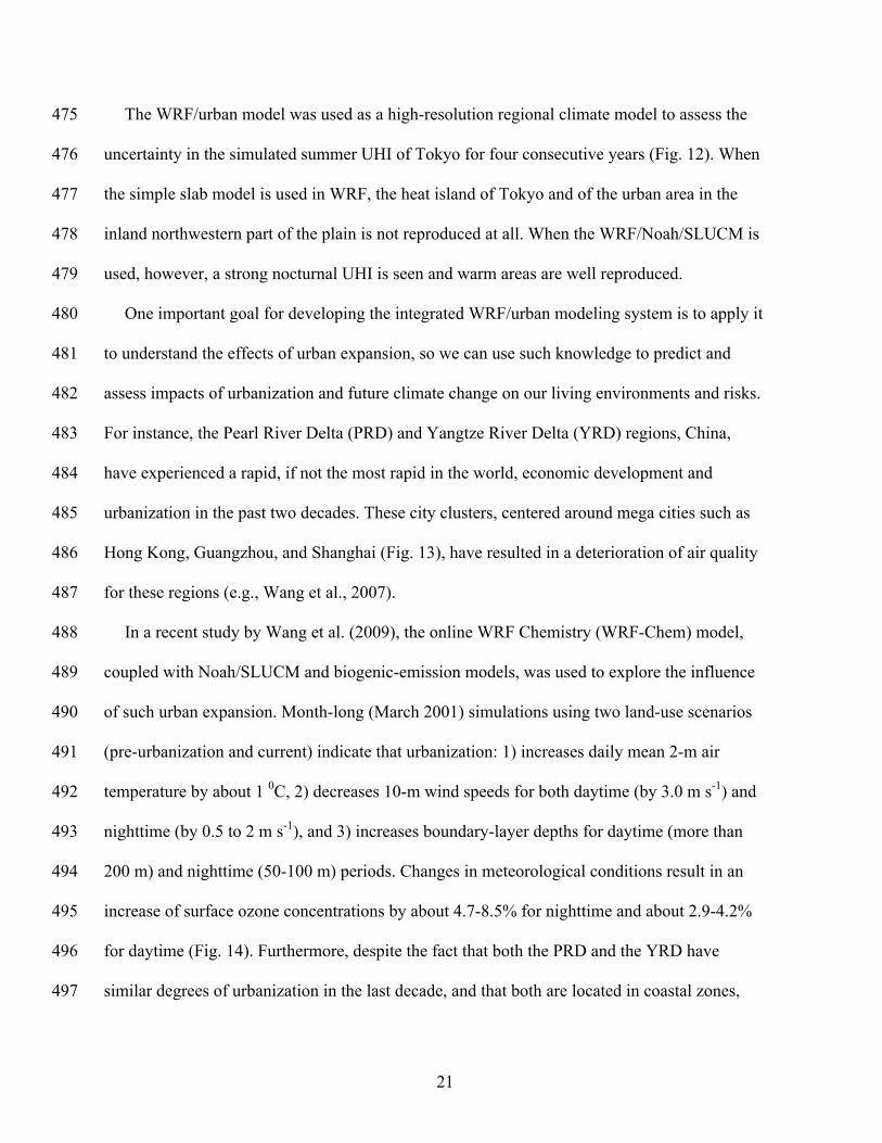
The WRF/urban model was used as a high-resolution regional climate model to assess the 475
uncertainty in the simulated summer UHI of Tokyo for four consecutive years (Fig. 12). When 476
the simple slab model is used in WRF, the heat island of Tokyo and of the urban area in the 477
inland northwestern part of the plain is not reproduced at all. When the WRF/Noah/SLUCM is 478
used, however, a strong nocturnal UHI is seen and warm areas are well reproduced. 479
One important goal for developing the integrated WRF/urban modeling system is to apply it 480
to understand the effects of urban expansion, so we can use such knowledge to predict and 481
assess impacts of urbanization and future climate change on our living environments and risks. 482
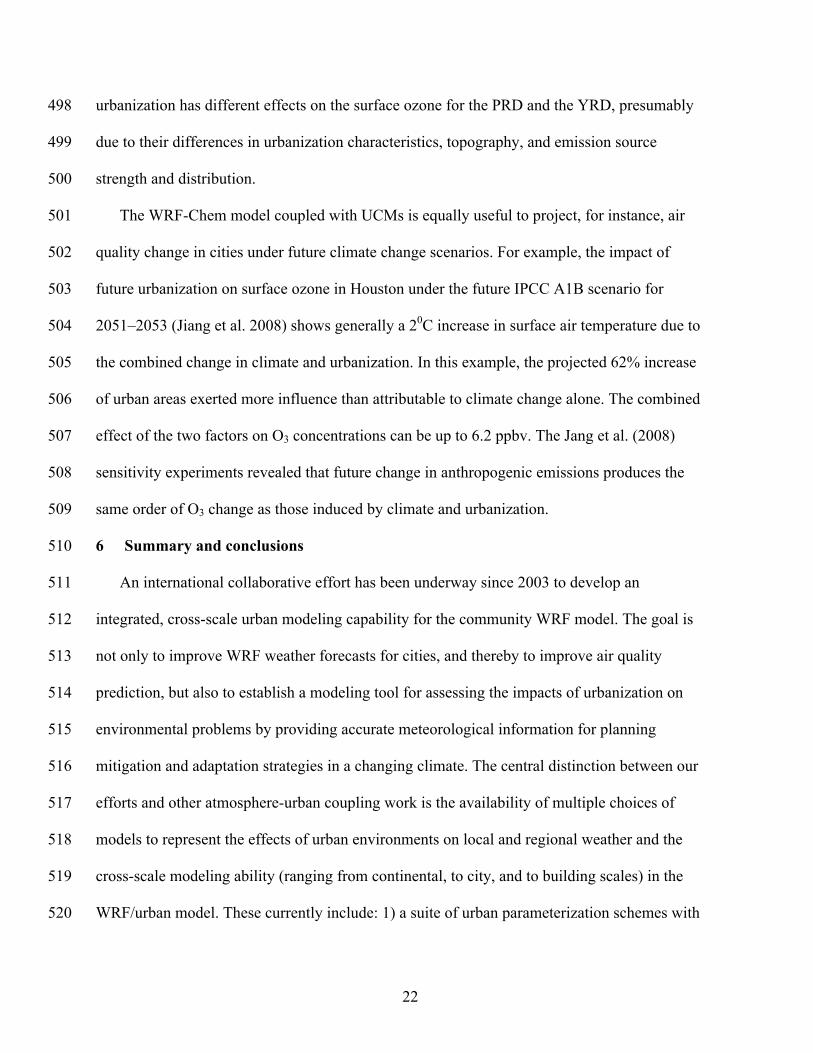
For instance, the Pearl River Delta (PRD) and Yangtze River Delta (YRD) regions, China, 483
have experienced a rapid, if not the most rapid in the world, economic development and 484
urbanization in the past two decades. These city clusters, centered around mega cities such as 485
Hong Kong, Guangzhou, and Shanghai (Fig. 13), have resulted in a deterioration of air quality 486
for these regions (e.g., Wang et al., 2007). 487
In a recent study by Wang et al. (2009), the online WRF Chemistry (WRF-Chem) model, 488
coupled with Noah/SLUCM and biogenic-emission models, was used to explore the influence 489
of such urban expansion. Month-long (March 2001) simulations using two land-use scenarios 490
(pre-urbanization and current) indicate that urbanization: 1) increases daily mean 2-m air 491
temperature by about 1 0C, 2) decreases 10-m wind speeds for both daytime (by 3.0 m s-1) and 492
nighttime (by 0.5 to 2 m s-1), and 3) increases boundary-layer depths for daytime (more than 493
200 m) and nighttime (50-100 m) periods. Changes in meteorological conditions result in an 494
increase of surface ozone concentrations by about 4.7-8.5% for nighttime and about 2.9-4.2% 495
for daytime (Fig. 14). Furthermore, despite the fact that both the PRD and the YRD have 496
similar degrees of urbanization in the last decade, and that both are located in coastal zones, 497
22
urbanization has different effects on the surface ozone for the PRD and the YRD, presumably 498
due to their differences in urbanization characteristics, topography, and emission source 499
strength and distribution. 500
The WRF-Chem model coupled with UCMs is equally useful to project, for instance, air 501
quality change in cities under future climate change scenarios. For example, the impact of 502
future urbanization on surface ozone in Houston under the future IPCC A1B scenario for 503
2051–2053 (Jiang et al. 2008) shows generally a 20C increase in surface air temperature due to 504
the combined change in climate and urbanization. In this example, the projected 62% increase 505
of urban areas exerted more influence than attributable to climate change alone. The combined 506
effect of the two factors on O3 concentrations can be up to 6.2 ppbv. The Jang et al. (2008) 507
sensitivity experiments revealed that future change in anthropogenic emissions produces the 508
same order of O3 change as those induced by climate and urbanization. 509
6 Summary and conclusions 510
An international collaborative effort has been underway since 2003 to develop an 511
integrated, cross-scale urban modeling capability for the community WRF model. The goal is 512
not only to improve WRF weather forecasts for cities, and thereby to improve air quality 513
prediction, but also to establish a modeling tool for assessing the impacts of urbanization on 514
environmental problems by providing accurate meteorological information for planning 515
mitigation and adaptation strategies in a changing climate. The central distinction between our 516
efforts and other atmosphere-urban coupling work is the availability of multiple choices of 517
models to represent the effects of urban environments on local and regional weather and the 518
cross-scale modeling ability (ranging from continental, to city, and to building scales) in the 519
WRF/urban model. These currently include: 1) a suite of urban parameterization schemes with 520

23
varying degrees of complexities, 2) a capability of incorporating in-situ and remote-sensing 521
data of urban land use, building characteristics, and anthropogenic heat and moisture sources, 522
3) companion fine-scale atmospheric and urbanized land data assimilation systems, and 4) 523
ability to couple WRF/urban to fine-scale urban T&D models and with chemistry models. 524
Inclusion of three urban parameterization schemes (i.e., bulk parameterization, SLUCM, 525
and BEP) provides users with options for treating urban surface processes. Parallel to an 526
international effort to evaluate 30 urban models, executed in offline 1-D mode, against site 527
observations (Grimmond et al., 2010), work is underway within our group to evaluate three 528
WRF urban models in coupled mode against surface and boundary layer observations from the 529
Texas Air Quality Study 2000 (TexAQS2000) field program in the greater Houston area, 530
Central California Ozone Study (CCOS2000), and Southern California Ozone Study 531
(SCOS1997). Choice of specific applications will dictate careful selection of different sets of 532
science options and available databases. For instance, the bulk parameterization and SLUCM 533
may be more suitable for real-time weather and air quality forecasts than the resource-534
demanding BEP. On the other hand, studying, for instance, the impact of air conditioning on 535
the atmosphere and in developing an adaptation strategy for planning the use of air 536
conditioning in less-developed countries in the context of intensified heat waves projected by 537
IPCC, will need to invoke the more sophisticated BEP coupled with the BEM indoor-outdoor 538
exchange model. 539
Initializing UCM state variables is a difficult problem, which has not yet received much 540
attention in the urban modeling community. Although in its early stage of development 541
(largely due to lack of appropriate data for its evaluation), u-HRLDAS may provide better 542
initial conditions for the state variables required by UCMs than the current solution that assigns 543
24
a uniform temperature profile for model grid points cross a city. Similarly, specification of 544
twenty-some UCPs will remain a challenge, due to the large disparity in data availability and 545
methodology for mapping fine-scale, highly variable data for the WRF modeling grid. 546
Currently the WRF pre-processor (WPS) is able to ingest: 1) high-resolution urban land-use 547
maps and to then assign UCPs based on a parameter table and 2) gridded UCPs, such as those 548
from NUDAPT (Ching et al., 2009). It would be useful to blend these two methods whenever 549
gridded UCPs are available. Bringing optimization algorithms together with UCMs and 550
observations, as recently demonstrated by Loridan et al. (2010), is a useful methodology to 551
identify a set of UCPs to which the performance of the UCM is most sensitive, and to 552
eventually define optimized values for those UCPs for a specific city. 553
Among these UCPs, anthropogenic heating (AH) has emerged as the most difficult 554
parameter to obtain. Methods to estimate AH from buildings, industry/manufacturing, and 555
transportation sectors have been developed (e.g., Sailor and Lu, 2004, Sailor and Hart, 2006, 556
Torcellini et al., 2008). Although data regarding the temporal and spatial distribution of waste 557
heat emissions from industry, buildings, and vehicle combustion do exist for most cities, 558
obtaining and processing these data are far from automated tasks. Nevertheless, the data 559
currently available for major US cities in NUDAPT provide examples of combining all AH 560
sources to create a single, hourly input for the WRF/urban model. 561
Evaluations and applications of this newly developed WRF/urban modeling system have 562
demonstrated its utility in studying air quality and regional climate. Preliminary results that 563
verify the performance of WRF/UCM for several major cities are encouraging (e.g., Chen et al., 564
2004, Holt and Pullen, 2007, Miao and Chen, 2008, Lin et al., 2008, Miao et al., 2009a, Miao 565
et al., 2009b, Wang et al., 2009, Tewari et al., 2010, Kusaka et al., 2009). They show that the 566
25
model is generally able to capture influences of urban processes on near-surface 567
meteorological conditions and on the evolution of atmospheric boundary-layer structures in 568
cities. More importantly, recent studies (Jiang et al., 2008, Wang et al., 2009, Tewari et al., 569
2010) have demonstrated the promising value of employing this model to investigate urban and 570
street-level plume T&D and air quality, and to predict impacts of urbanization on our living 571
environments and for risks in the context of global climate change. 572
While this WRF/urban model has been released (WRF V3.1, April 2009), except for the 573
BEM model that is in the final stages of testing, much work still remains to be done. We 574
continue to: further improve the UCMs, explore new methods of blending various data sources 575
to enhance the specification UCPs, increase the coverage of high resolution data sets, 576
particularly enhancing anthropogenic heating and moisture inputs, and link this physical 577
modeling system with, for instance, human-response models and decision support systems. 578
579 Acknowledgements 580
581 This effort was supported by the US Air Force Weather Agency (AFWA), NCAR FY07 582
Director Opportunity Fund, Defense Threat Reduction Agency (DTRA) Coastal-urban project, 583
and National Science Foundation (Grants 0710631 and 0410103). This work was also 584
supported by the National Natural Science Foundation of China (Grant Nos. 40875076, 585
U0833001, 40505002, and 40775015). Computer time was provided by NSF MRI Grant CNS-586
0421498, NSF MRI Grant CNS-0420873, NSF MRI Grant CNS-0420985, the University of 587
Colorado, and a grant from the IBM Shared University Research (SUR) program.588
26
589
References 590 591
Allwine, K, J., J.H. Shinn, G.E. Streit, K. L. Clawson, and M. Brown, 2002. Overview of 592
URBAN 2000: A multiscale field study of dispersion through an urban environment. 593
Bull. Amer. Meteor. Soc., 83, 521-536. 594
Allwine, K. J., and Coauthors, 2004: Overview of Joint Urban 2003: An atmospheric 595
dispersion study in Oklahoma City. AMS Symposium on planning, nowcasting and 596
forecasting in urban zone (on CD). Seattle, WA, Amer. Meteor. Soc. 597
Best, M. J., 2005: Representing urban areas within operational numerical weather prediction 598
models. Bound.-Layer Meteorol., 114, 91-109. 599
Bougeault, P. and Lacarrère, P. 1989. Parameterization of orography-induced turbulence in a 600
mesobeta-scale model. Mon. Wea. Rev. 117: 1872-1890. 601
Brown, M. J., 2004: Urban dispersion—Challenges for fast response modeling. Preprints, Fifth 602
Conf. on Urban Environment, Vancouver, BC, Canada, Amer. Meteor. Soc., J5.1. 603
[Available online at http://ams.confex.com/ams/AFAPURBBIO/techprogram/ 604
paper_80330.htm.] 605
Burian, S.J., S.W. Stetson, W. Han, J. Ching, and D. Byun, 2004: High‐resolution dataset of 606
urban canopy parameters for Houston, Texas. Preprint proceedings, Fifth 607
Symposium on the Urban Environment, Vancouver, BC, Canada, American 608
Meteorological Society, Boston, 23‐26 August, 9 pages. 609
Burian, S.J., and Co-authors, 2006: Emerging urban databases for meteorological and 610
dispersion. Sixth Symposium on the Urban Environment, Atlanta GA Jan 28-Feb 2, 611
American Meteorological Society, Boston, Paper 5.2. 612
27
Burian, S.J., M.J. Brown, N. Augustus, 2007: Development and assessment of the second 613
generation National Building Statistics database. Seventh Symposium on the Urban 614
Environment, San Diego, CA Sep 10-13, American Meteorological Society, Boston, 615
Paper 5.4. 616
Chen, F., and Coauthors, 1996: Modeling of land-surface evaporation by four schemes and 617
comparison with FIFE observations. J. Geophys. Res., 101, 7251-7268. 618
Chen, F., Z. Janjic, and K. Mitchell, 1997: Impact of atmospheric surface layer 619
parameterization in the new land-surface scheme of the NCEP mesoscale Eta numerical 620
model. Bound.-Layer Meteorol., l85, 391-421. 621
Chen, F., and J. Dudhia, 2001: Coupling an advanced land-surface/hydrology model with the 622
Penn State/NCAR MM5 modeling system. Part I: Model implementation and sensitivity. 623
Mon. Wea. Rev., 129, 569-585. 624
Chen, F, H. Kusaka, M. Tewari, J.-W. Bao, and H. Harakuchi, 2004: Utilizing the coupled 625
WRF/LSM/urban modeling system with detailed urban classification to simulate the 626
urban heat island phenomena over the Greater Houston area. Preprints, Fifth Symp. on the 627
Urban Environment, Vancouver, BC, Canada, Amer. Meteor. Soc., 9-11. [Available 628
online at http://ams.confex.com/ams.pdfpapers/79765.pdf.] 629
Chen, F., and Coauthors, 2007: Evaluation of the characteristics of the NCAR high-resolution 630
land data assimilation system. J. Appl. Meteor., 46, 694-713. 631
Ching, J., and Coauthors, 2009: National Urban Database and Access Portal Tool, NUDAPT, 632
Bull. American Meteorol. Soc., Vol. 90, Issue 8, pages 1157-1168. 633

28
Coirier, W. J., D. M. Fricker, M. Furmanczyk, and S. Kim, 2005: A computational f luid 634
dynamics approach for urban area transport and dispersion modeling. Environ. Fluid 635
Mech., 5, 443–479. 636
Dupont, S., T.L. Otte, and J.K.S. Ching, 2004: Simulation of meteorological fields within and 637
above urban and rural canopies with a mesoscale model (MM5) Boundary Layer Meteor., 638
2004 113: 111-158. 639
Ek, M. B., and Coauthors, 2003: Implementation of Noah land surface model advances in the 640
National Center for Environmental Prediction operational mesoscale Eta model. J. 641
Geophys. Res., 108 (D22), 8851, doi:10.1029/2002JD003296. 642
Feddema, J., K. Oleson and G. Bonan 2006. Developing a global database for the CLM urban 643
model, Sixth Symposium on the Urban Environment, 86th AMS Annual Meeting, 644
Atlanta, GA, February 1. 645
FERC 2006, “Form 714 - Annual Electric Control and Planning Area Report Data”, Federal 646
Energy Regulatory Commission, http://www.ferc.gov/docs-filing/eforms/form-647
714/data.asp. 648
Grell, G., and Coauthors, 2005: Fully coupled online chemistry within the WRF model. Atmos. 649
Environ., 39, 6957-6975 650
Grimmond, CSB, and Coauthors, 2010: The International Urban Energy Balance Models 651
Comparison Project: First results from Phase 1. J. Appl. Meteorol. Climatol., in press. 652
Grimmond CSB, Salmond JA, Oke TR, Offerle B, Lemonsu A. 2004. Flux and turbulence 653
measurements at a densely built-up site in Marseille: Heat, mass (water and carbon 654
dioxide), and momentum. Journal of Geophysical Research, Atmospheres 109: D24, D24 655
101, 19pp doi:10.1029/2004JD004936. 656
29
Heiple, SC and DJ Sailor, 2008: Using building energy simulation and geospatial modeling 657
techniques to determine high resolution building sector energy consumption profiles. 658
Energy and Buildings, 40, 1426-1436. 659
Holt, T., and J. Pullen, 2007: Urban Canopy Modeling of the New York City Metropolitan 660
Area: A Comparison and Validation of Single- and Multilayer Parameterizations. Mon. 661
Wea. Rev., 135, 1906–1930. 662
Janjic, Z. I., 1994: The step-mountain eta coordinate: Further development of the convection, 663
viscous sublayer, and turbulent closure schemes. Mon. Wea. Rev., 122, 927–945. 664
Jiang, X.Y., C. Wiedinmyer, F. Chen, Z.L. Yang, and J. C. F. Lo, 2008: Predicted Impacts of 665
Climate and Land-Use Change on Surface Ozone in the Houston, Texas, Area. J. 666
Geophys. Res., 113, D20312, doi:10.1029/2008JD009820. 667
Kusaka, H., H. Kondo, Y. Kikegawa, and F. Kimura, 2001: A simple single-layer urban 668
canopy model for atmospheric models: Comparison with multi-layer and slab models. 669
Bound.-Layer Meteor., 101, 329-358. 670
Kusaka, H., and F. Kimura, 2004: Coupling a single-layer urban canopy model with a simple 671
atmospheric model: Impact on urban heat island simulation for an idealized case. J. 672
Meteor. Soc. Japan, 82, 67-80. 673
Kusaka, H., and Coauthors, 2009: Performance of the WRF model as a high resolution regional 674
climate model: Model intercomparison study. Proc. ICUC-7 (in CD-ROM). 675
Lemonsu, A. and V. Masson, 2002: Simulation of a summer urban Breeze over Paris. Bound.-676
Layer Meteorol., 104, 463-490. 677
30
Lemonsu A, Grimmond CSB, Masson V. 2004. Modelling the surface energy balance of the 678
core of an old mediterranean city: Marseille. Journal of Applied Meteorology, 43: 312–679
327. 680
Leung, L. R., Y. H. Kuo, et al. (2006). "Research Needs and Directions of Regional Climate 681
Modeling Using WRF and CCSM." Bull. American Meteorol. Soc., 87, 1747-1751. 682
Lin, C-Y, and Coauthors, 2008: Urban Heat Island effect and its impact on boundary layer 683
development and land-sea circulation over northern Taiwan, Atmospheric Environment, 684
42, 5635-5649. doi:10.1016. 685
Liu, Y., F. Chen, T. Warner, and J. Basara, 2006: Verification of a Mesoscale Data-686
Assimilation and Forecasting System for the Oklahoma City Area During the Joint Urban 687
2003 Field Project. J. Appli. Meteorol., 45, 912–929. 688
Lo, J.C.F., A.K.H. Lau, F. Chen, J.C.H. Fung, and K.K.M. Leung, 2007: Urban Modification 689
in a Mesoscale Model and the Effects on the Local Circulation in the Pearl River Delta 690
Region. J. Appl. Meteorol. Climtol., 46, 457–476. 691
Loridan T, and Coauthors, 2010. Trade-offs and responsiveness of the single-layer urban 692
parameterization in WRF: an offline evaluation using the MOSCEM optimization 693
algorithm and field observations. Submitted to the Quarterly Journal of the Royal 694
Meteorological Society. 695
Martilli A., Clappier A., and Rotach M. W. 2002. An urban surface exchange parameterization 696
for mesoscale models. Bound.-Layer Meteorol., 104: 261-304. 697
Martilli A., and R. Schmitz, 2007, Implementation of an Urban Canopy Parameterization in 698
WRF-chem. Preliminary results. Seventh Symposium on the Urban Environment of the 699
American Meteorological Society, San Diego, USA, 10-13 September. 700

31
Miao, S., and F. Chen, 2008: Formation of horizontal convective rolls in urban areas. Atm. 701
Res., 89(3): 298-304. 702
Miao, S., F. Chen, M. A. LeMone, M. Tewari, Qingchun Li, and Yingchun Wang, 2009a: An 703
observational and modeling study of characteristics of urban heat island and boundary 704
layer structures in Beijing. J. Appl. Meteorol. Climtol, 48(3): 484–501. 705
Miao, S., F. Chen, Q. Li, and S. Fan, 2009b: Impacts of urbanization on a summer heavy 706
rainfall in Beijing, The seventh International Conference on Urban Climate: Proceeding, 707
29 June - 3 July 2009, Yokohama, Japan, B12-1. 708
Mitchell, K.E., and Coauthors, 2004: The multi-institution North American Land Data 709
Assimilation System (NLDAS): Utilizing multiple GCIP products and partners in a 710
continental distributed hydrological modeling system. J. Geophys. Res., 109, D07S90, 711
doi:10.1029/2003JD003823. 712
Otte, T. L., A. Lacser, S. Dupont, and J. K. S. Ching, 2004: Implementation of an urban 713
canopy parameterization in a mesoscale meteorological model. J. Appl. Meteor., 43, 1648-714
1665. 715
Nicholls, R.J. and Coauthors, 2007: Screening Study: Ranking Port Cities with High Exposure 716
and Vulnerability to Climate Extremes: Interim Analysis: Exposure Estimates. OECD 717
2007. (www.oecd.org/env/workingpapers). 718
Oleson, K.W., Bonan, G.B., Feddema, J., Vertenstein, M. and Grimmond, C.S.B., 2008: An 719
urban parameterization for a global climate model: 1. Formulation & evaluation for two 720
cities, J. Appl. Meteorol. Climatol. 47,1038-1060. DOI: 10.1175/2007JAMC1597.1 721
Prusa, J.M., P.K. Smolarkiewicz, and A.A. Wyszogrodzki, 2008: EULAG, a computational 722
model for multiscale flows. Computers and Fluids, 37, 1193–1207. 723

32
Rotach, M. W., and Coauthors, 2005: BUBBLE – an Urban Boundary Layer Meteorology 724
Project. Theor. Appl. Climatol. 81, 231–261. DOI 10.1007/s00704-004-0117-9 725
Sailor, DJ and L Lu, 2004: A top-down methodology for developing diurnal and seasonal 726
anthropogenic heating profiles for urban areas. Atmos. Environ., 38, 2737-2748. 727
Sailor, D.J, M. Hart, 2006: An anthropogenic heating database for major U.S. cities, Sixth 728
Symposium on the Urban Environment, Atlanta GA Jan 28-Feb 2, American 729
Meteorological Society, Boston, Paper 5.6. 730
Salamanca, F., Krpo, A., Martilli, A., Clappier, A., 2009, A new building energy model 731
coupled with an Urban Canopy Parameterization for urban climate simulations – Part I. 732
Formulation, verification and sensitivity analysis of the model. Theoretical and Applied 733
Climatology. DOI 10.1007/s00704-009-0142-9. 734
Salamanca, F., Martilli, A., 2009, A new building energy model coupled with an Urban 735
Canopy Parameterization for urban climate simulations – Part II. Validation with one 736
dimension off-line simulations. Theoretical and Applied Climatology. DOI 737
10.1007/s00704-009-0143-8. 738
Skamarock, W. C., and Coauthors, 2005: A description of the Advanced Research WRF 739
version 2. NCAR Tech. Note TN-468+STR, 88 pp. [Available from NCAR, P. O. Box 740
3000, Boulder, CO 80307.] 741
Smolarkiewicz, P. K., and Coauthors, 2007: Building resolving large-eddy simulations and 742
comparison with wind tunnel experiments. J. Comput. Phys., 227, 633-653. 743
Taha, H, 1999: Modifying a mesoscale meteorological model to better incorporate urban heat 744
storage: A bulk-parameterization approach. Journal of Applied Meteorology, 38, 466-745
473. 746
33
Taha, H. and R. Bornstein, 1999: Urbanization of meteorological models: Implications on 747
simulated heat islands and air quality. International Congress of Biometeorology and 748
International Conference on Urban Climatology (ICB-ICUC) Conference, 8-12 749
November 1999, Sydney Australia. 750
Taha, H., and J.K.S. Ching, 2007: UCP / MM5 Modeling in conjunction with NUDAPT: 751
Model requirements, updates, and applications, Seventh Symposium on the Urban 752
Environment, San Diego, CA Sep 10-13, American Meteorological Society, Boston, 753
Paper 6.4. 754
Taha, H., 2008a: Urban surface modification as a potential ozone air-quality improvement 755
strategy in California: A mesoscale modeling study. Boundary-Layer Meteorology, Vol. 756
127, 2, 219-239. doi:10.1007/s10546-007-9259-5. 757
Taha, H., 2008b: Meso-urban meteorological and photochemical modeling of heat island 758
mitigation. Atmospheric Environment, 42, 8795-8809. 759
doi:10.1016/j.atmosenv.2008.06.036 760
Tewari, M., H. Kusaka, F. Chen, W. J. Coirier, S. Kim, A, Wyszogrodzki, T. T. Warner, 2010. 761
Impact of coupling a microscale computational fluid dynamics model with a mesoscale 762
model on urban scale contaminant transport and dispersion. Atmos. Res. In Press. 763
Torcellini, P, M Deru, B Griffith, K Benne, M Halverson, D Winiarski, and DB Crawley, 764
2008: DOE Commercial Building Benchmark Models, 15 pp. 765
United Nations, 2007: World Urbanization Prospects: The 2007 Revision, 766
http://esa.un.org/unup. 767
34
Vrugt, JA, Gupta HV, Bastidas LA, Bouten W. 2003. Effective and efficient algorithm for 768
multiobjective optimization of hydrological models. Water Resources Research 39: 769
12 014, doi:10.1029/2002WR001746. 770
Wang, X. M., W. S. Lin, L. M. Yang, R. R. Deng, and H. Lin, 2007: A numerical study of 771
influences of urban land-use change on ozone distribution over the Pearl River Delta 772
Region, China. Tellus, 59B, 633-641. 773
Wang, X.M., and Coauthors, 2009: Impacts of weather conditions modified by urban 774
expansion on surface ozone: Comparison between the Pearl River Delta and Yangtze 775
River Delta regions, Adv. in Atmos. Sci., 2009b, 26,962-972. 776
Wyszogrodzki A.A., and P.K. Smolarkiewicz, 2009: Building resolving large-eddy simulations 777
(LES) with EULAG. Academy Colloquium on Immersed Boundary Methods: Current 778
Status and Future Research Directions, 15-17 June 2009, Academy Building, 779
Amsterdam, the Netherlands. 780
Zhang, C. L., F. Chen, S. G. Miao, Q. C. Li, X. A. Xia, and C. Y. Xuan (2009), Impacts of 781
urban expansion and future green planting on summer precipitation in the Beijing 782
metropolitan area. J. Geophys. Res., 114, D02116, doi:10.1029/2008JD010328. 783
784

35
784
Table 1. Urban canopy parameters currently in WRF for three urban land-use categories: 785 low-intensity residential, high-intensity residential, and industrial and commercial. The last 786 two columns indicate if a specific parameter is used in SLUCM and BEP, and the last three 787 parameters are exclusively used in BEP. 788
789 790
Specific Values for Parameter Unit Low
intensity residential
High intensity residential
Industrial, commercial
SLUCM BEP
h (Building Height)
m 5 7.5 10 Yes No
lroof (Roof Width )
m 8.3 9.4 10 Yes No
lroad (Road Width)
m 8.3 9.4 10 Yes No
AH (Anthropogenic Heat)
W m-2 20 50 90 Yes No
(Urban fraction)
Fraction 0.5 0.9 0.95 Yes Yes
CR (Heat capacity of roof)
J m-3 K-1 1.0E6 1.0E6 1.0E6 Yes Yes
CW (Heat capacity of building wall)
J m-3 K-1 1.0E6 1.0E6 1.0E6 Yes Yes
CG (Heat capacity of road)
J m-3 K-1 1.4E6 1.4E6 1.4E6 Yes Yes
λR (Thermal Conductivity of roof)
J m-1s-1K-1 0.67 0.67 0.67 Yes Yes
λW (Thermal Conductivity of building wall)
J m-1s-1K-1 0.67 0.67 0.67 Yes Yes
λG (Thermal Conductivity of road)
J m-1s-1K-1 0.4004 0.4004 0.4004 Yes Yes
αR (Surface Albedo of roof)
Fraction 0.20 0.20 0.20 Yes Yes
αW (Surface Albedo of building wall)
Fraction 0.20 0.20 0.20 Yes Yes
αG (Surface Albedo of road)
Fraction 0.20 0.20 0.20 Yes Yes
εR (Surface emissivity of roof)
- 0.90 0.90 0.90 Yes Yes

36
εW (Surface emissivity of building wall)
- 0.90 0.90 0.90 Yes Yes
εG (Surface emissivity of road)
- 0.95 0.95 0.95 Yes Yes
Z0R (Roughness length for momentum over roof)
m 0.01 0.01 0.01 Yes* Yes
Z0W (Roughness length for momentum over building wall)
m 0.0001 0.0001 0.0001 No* No
Z0G (Roughness length for momentum over road)
m 0.01 0.01 0.01 No* Yes
b) Parameters used only in BEP Street Parameters
Directions from North (degrees)
Directions from North (degrees)
Directions from north (degrees)
No Yes
0 90 0 90 0 90 W (Street Width)
m 15 15 15 15 15 15
B (Building Width)
m 15 15 15 15 15 15
h (Building Heights)
m Height % Height % Height %
5 50 10 3 5 30 10 50 15 7 10 40 20 12 15 50 25 18 30 20 35 18 40 12 45 7 50 3 791 792
*Note: For SLUCM, if the Jurges’ formulation is selected instead of Monin-Obukhov 793 formulation (a default option in WRF V3.1), Z0W and Z0G are not used.794
37
Figure Captions 795 796
Figure 1. Overview of the integrated WRF/urban modeling system, which includes urban-797
modeling data-ingestion enhancements in the WRF Preprocessor System (WPS), a suite of 798
urban modeling tools in the core physics of WRF V 3.1, and its potential applications. 799
800
Figure 2. A schematic of the single-layer UCM (SLUCM, on the left-hand side) and the multi-801
layer BEP models (on the right-hand side). 802
803
Figure 3. Simulated vertical profiles of nighttime temperature above a city and a rural site 804
upwind of the city. Results obtained with WRF/BEP for a 2-D simulation (from Martilli and 805
Schmitz, 2007). 806
807
Figure 4. Kinematic sensible heat fluxes: measured (solid line); computed offline with 808
BEP+BEM and air conditioning working 24-h a day (ucp-bemac); with BEP+BEM and air 809
conditioning working only from 0800 to 2000 LST (ucp-bemac*); with BEP+BEM, but 810
without air conditioning (ucp-bem); and with the old version BEP. Results are at 18 m for a 811
three-day period during the BUBBLE campaign (from Salamanca and Martilli, 2009). 812
813
Figure 5. Schematic representation of the coupling between the mesoscale WRF and the fine-814
scale urban T&D EULAG model. 815
816
Figure 6: Contours are the density of SF6 tracer gas (in parts per thousand) 60 minutes after the 817
third release, simulated by CFD-urban using: a) single sounding observed at the Raging Waters 818
site and (b) WRF 12-h forecast. Dots represent observed density (in same scale as in scale bar) 819
at sites throughout the downtown area of Salt Lake City (from Tewari et al. 2010). 820
821
Figure 7. Dispersion footprint for IOP6 0900 CDT release from source located at Botanical 822
Gardens (near Sheridan & Robinson avenues, Oklahoma City, Oklahoma) calculated with 823
WRF/EULAG. 824
825
38
Figure 8. Noah/SLUCM simulated differences in 4th-layer road temperature (K), valid at 1200 826
UTC 23 August 2006 for Houston, Texas, between the control simulation with 20-month spin-827
up time and a sensitivity simulation with: a) six-month, b) two-month, c) one-month, and d) 828
14-day spin-up times. 829
830
Figure 9. Land use and land cover in the Greater Houston area, Texas, based on 30-m Landsat 831
from the NLCD 1992 data. 832
833
Figure 10: Optimum roof albedo values (αr) identified by MOSCEM, when considering the 834
RMSE (W m-2) for and with forcing and evaluation data from Marseille. 835
836
Figure 11. The diurnal variation of: (a) temperature (°C), as observed (obs), modeled 2-m air 837
temperature (t2) and within the canyon (T2C), modeled aggregated land surface (TSK), and 838
facet temperatures for roof (TR), wall (TB) and ground (TG); (b) observed (obs) and modeled 839
10-m wind speed (wsp) and simulated wind-speed within the urban canyon in m s-1; and (c) 840
observed (obs) and modeled (q2) 2-m specific humidity (g kg-1). Variables were averaged over 841
high-density urban area stations for Beijing (from Miao et al., 2009a). 842
843
Figure 12. Monthly mean surface air temperature at 2 m in Tokyo area at 0500 JST in August 844
averaged for 2004-2007: (a) AMeDAS observations, (b) from WRF/Slab model, and (c) from 845
WRF/SLUCM (from Kusaka et al., 2009). 846
847
Figure 13. Urban land-use change in the PRD and YRD regions, China, marked in red from 848
pre-urbanization (1992-93) and current (2004): a) WRF-Chem domain with 12-km grid 849
spacing; b) 1992-1993 USGS data for PRD, c) 2004 MODIS data for YRD, d) 1992-1993 850
USGS data for PRD, and e) 2004 MODIS data for YRD (from Wang et al., 2009). 851
852
Figure 14. Difference of surface ozone (in ppbv) and relative 10-m wind vectors: (a) daytime, 853
(b) nighttime (from Wang et al., 2009). 854