The Indecisive Shopper:

Incorporating Choice Paralysis

into the Multinomial Logit Model

by

Anisha Patel

An honors thesis submitted in partial fulfillment

of the requirements for the degree of

Bachelors of Science

Undergraduate College

Leonard N. Stern School of Business

New York University

May 2014

Marti G. Subrahmanyam Rene Caldentey, Srikanth JagabathulaFaculty Adviser Thesis Advisers

1

The Indecisive Shopper: Incorporating Choice Paralysis into the

Multinomial Logit Model

Anisha Patel, Rene Caldentey, Srikanth Jagabathula

Stern School of Business

New York University

Abstract

In this paper, we investigate choice paralysis and its implications on business decision mak-

ing. Choice paralysis is the notion that too many options can paralyze a consumer and make

them more prone to not purchasing anything at all or reverting to some default option. Using

supermarket panel data, we find empirical evidence of this phenomenon; specifically, we find

that consumers are more likely to purchase their more preferred (default) option as the cardi-

nality of the assortment (offered set) increases. Interestingly, and despite the fact that there is

extensive research in consumer psychology that has reported and studied choice paralysis , most

popular consumer choice models –such as the Multinomial Logit model (MNL)– are not able

to capture this type of consumer purchasing behavior. Normally, these consumer choice models

assume that buyers are rational utility-maximizer agents and, under this paradigm, a retailer

who increases the offered set should expect to see an increase in the likelihood of consumers

buying a product or switching more from their default brand.

In order to bridge this gap, we aim to make two contributions: (a) provide empirical val-

idation and quantification of this choice paralysis phenomenon, and (b) modify the existing

MNL model to capture the implications of this effect. First, we analyze real-world panel data

of yogurt, coffee, milk, and shampoo sales to test for the presence of the choice paralysis effect.

Our results provide empirical validation in varying degrees across products for the choice paral-

ysis phenomenon. Specifically, we find a negative quadratic relationship between a customers’

likelihood to switch from their default brand as a function of assortment size.

Next, we propose a modification to the MNL model that aims at capturing this choice

paralysis and at the same time preserving its parsimonious nature. Our proposed model builds

upon two fundamental postulates. First, we assume that consumers have a limited capacity

(or patience) to evaluate an assortment of products and as a result they can only assess the

utility of a subset of them. We refer to this subset as the consumer’s consideration set and

view its cardinality as a measure of the consumer’s cognitive budget to evaluate the available

options. To capture heterogeneity in the consumers’ population, we model the cardinality of

the consideration set as a non-negative integer random variable. Our second postulate is that

consumers penalize the utility of the products in their consideration set with a factor that

increases with the number of products that are not in this subset. The premise behind this

postulate is that a consumer who is making a choice decision that only involves a subset of the

available products will feel that her decision is “premature” and will leave her second-guessing

whether she really made the best selection. We assume that this remorse increases with the

number of unevaluated products and acts as a disutility on those products in the consideration

set.

Combining the cognitive budget and remorse effects, we propose a variation of the MNL

model that is consistent with consumers’ choice paralysis and use this model to (i) study optimal

inventory and assortment planning decisions and to (ii) propose how these results can be used

to quantify the revenue impact of not accounting for this behavioral phenomenon.

3

Acknowledgements

This final paper would not have been possible without the guidance and support of a number of

incredible people.

First and foremost, I owe my deepest thanks to my thesis advisers, Professor Caldentey and Pro-

fessor Jagabathula, who not only provided the utmost support throughout the entire process but

worked hand-in-hand with me each week for hours at a time to ensure I had an enriching experience

and a quality product.

Thank you to Professor Subrahmanyam for creating the Senior Honors Program and providing such

a unique opportunity to pursue year-long research as an undergraduate. Thank you also to Jessie

Rosenzweig for making our trip to Omaha to visit Warren Buffett through this program possible.

To my wonderful friends, Carolyn, Taehoon, Giuseppe, and Vasudha, thank you so much for your

support. Whether it was giving me feedback on my ideas, offering help as I tried to learn Python,

staying up with me on the late nights, helping me come up with a thesis title, or coming to Stern

early on a Friday morning just to support me for my final presentation, I could not ask for a more

dedicated or caring group of friends to get me thorugh this year-long endeavor.

Aside from CodeAcademy, I would also like to thank my cousin, Anand, for his help as I took on

the formidable task of learning Python this past semester to do data analysis for my research. You

saved me from countless hours of trial and error testing and debugging.

Finally, I want to thank my parents and brother for always being my support network, regardless

of distance. No matter the endevaor, they have always encouraged me to follow my interests and

constantly challenge myself to go above and beyond.

It is your endless love and support that made this final product possible.

4

Contents

1 Introduction 6

2 Literature Review: Psychological Research on Choice 7

3 Data Analysis: Empirical Evidence of Choice Paralysis 9

3.1 Data Analysis Method: Rethinking the MNL . . . . . . . . . . . . . . . . . . . . . . 9

3.2 Data Analysis Results: Yogurt . . . . . . . . . . . . . . . . . . . . . . . . . . . . . . 11

3.3 Data Analysis Results: Coffee . . . . . . . . . . . . . . . . . . . . . . . . . . . . . . . 12

3.4 Data Analysis Results: Milk . . . . . . . . . . . . . . . . . . . . . . . . . . . . . . . . 14

3.5 Data Analysis Results: Shampoo . . . . . . . . . . . . . . . . . . . . . . . . . . . . . 15

3.6 Implications of the Results . . . . . . . . . . . . . . . . . . . . . . . . . . . . . . . . . 16

4 Background: The Multinomial Logit Model 17

5 The Multinomial Logit Model with Choice Paralysis (MNL-CP) 20

5.1 MNL-CP Model with Homogeneous Products . . . . . . . . . . . . . . . . . . . . . . 23

6 Application and Key Takeaways 25

7 Further Research 26

5

1 Introduction

Revenue management practices began with the airlines in the 1980s and have since fundamentally

changed the way companies approach decision-making in respect to the “what, when, where, and

how” of selling products to their target consumers. A critical component to this decision-making

is predicting consumers’ buying decisions through consumer choice models. These models aim

to simplistically but effectively reflect the consumer decision-making process and forecast their

purchase decisions. Companies then use these models to make key product decisions: the price of

the product, the amount of product to hold in inventory, the channels through which to sell the

product, and the potential markdown strategy over a product’s life cycle.

The success and profitability that these consumer choice models can bring to a company is entirely

contingent upon these models’ ability to accurately predict consumer behavior. However, this is

precisely where the issue lies. Existing consumer choice models fail to capture elements of choice

paralysis found in consumer behavior, resulting in sub-optimal pricing decisions and failure to

maximize revenue potential. While it is impossible to fully capture the internal consumer decision-

making process, there is overwhelming psychological research on changes in consumer behavior

when faced with choice that suggests existing consumer choice models are currently overlooking an

important component of consumer decision-making. Specifically, research has shown that there is

such a thing as too much choice, or “choice overload,” and it can be debilitating for consumers.

When companies provide too many offerings, consumers can become paralyzed by the number of

options in front of them and find it difficult or impossible to make a purchasing decision. Consumers

either must expend extra time and energy to make a selection, diminishing the enjoyment of their

overall purchasing experience and potentially reducing their likelihood to return to the business, or

they choose not to make any purchase decision at all. Both results have serious negative implications

for companies and their revenues.

In this research, we aim to quantify this choice overload phenomenon and propose a model that

aims to incorporate these currently uncaptured effects. As they currently stand, the underlying

assumptions of popular consumer choice models, specifically the Multinomial Logit (MNL), fail

to account for the choice paralysis effect. By developing and testing a model that takes existing

consumer choice models and incorporates this change in consumer behavior when faced with excess

choice, we hope to bridge the gap between these two, currently incompatible streams of thought.

The contents of this paper will look to further investigate the implications of psychological research

on choice paralysis, test for empirical evidence of this phenomenon in data, and propose a model

that more precisely quantifies the impact of this phenomenon on a consumer’s purchasing decisions.

The model can then be applied back to our original data, allowing us to more accurately determine

the effect the number of choices available has on a consumer’s likelihood to buy. We will conclude by

suggesting how companies can use this research to reevaluate how they make inventory management

and assortment planning decisions and find a balance between providing a healthy selection of

products to consumers and maximizing revenue.

6

2 Literature Review: Psychological Research on Choice

As Schwartz (2004) points out in The Paradox of Choice, we live our lives under the impression

that choice is good and therefore assume that more choice must be better. However, what if there

were such a thing as “too much choice” and it can actually make us unhappy? Such a notion seems

absurd, given our fundamental belief in the freedom to choose. Choice is an essential component to

our autonomy and, therefore, our well-being. However, in recent years, psychologists have looked

further into the matter and increasingly shown that, just as too little choice can be bad, too much

choice can be equally detrimental. More can actually be less. The implications of this finding

are huge, particularly for businesses who have constantly sought out to expand our choices and

selections in line with our desire to have more and more options. Knowing how many choices would

be “just right” is going to be critically important for companies trying to maximize revenue and

entice customers to return for future purchases. If the effect of consumer response to the number

of choices available can be quantified, companies can accordingly refine the way they operate and

prioritize the offerings they provide to create a better and more profitable shopping experience.

It is estimated that an average individual makes 72 decisions a day, meaning each of us is working

with limited time and energy to make each decision (see Cutrone, 2013). As a result, studies

conducted on the topic of consumer choice have shown that too many options burden consumers

and can negatively impact their decision-making process. Specifically, when consumers are faced

with choice overload, one of two consequences inevitably result: consumers make poor decisions

and are likely dissatisfied with their shopping experience, or consumers are paralyzed by the choice

in front of them and make no purchase at all (see chapter 1 in Schwartz, 2004). Of the customers

that do purchase, they will either make a premature selection that leaves them second-guessing

whether they really made the best selection, or they will take the time to evaluate all the options

but derive diminished utility from the purchase because of the time and energy that went into

making that choice (see chapter 1 in Schwartz, 2004)

Meanwhile, paralyzed customers make no choice at all and leave the purchasing process both

empty-handed and fatigued from their experience. This phenomenon is known as choice paralysis,

and it was best illustrated in effect in Iyengar (2010) famous jam experiment. Iyengar set up a

booth of jam samples in a California gourmet market and alternated the selection between six

jams and 24 jams every few hours. Her study discovered that 60% of customers were drawn to the

large assortment while only 40% stopped by the small assortment. This behavior is very much in

line with our common perception that more choice is better. However, when it came to making

the actual purchasing decision, 30% of the people who stopped at the small assortment made a

purchase, while only 3% of those who had the large assortment to choose from bought a jam. This

study, as Iyengar aptly puts it, shows that “the presence of choice might be appealing as a theory,

but in reality, people might find more and more choice to actually be debilitating” (for more details

see chapter 6 in Iyengar, 2010). In addition, marketing research has found that those faced with

too many choices, even in the face of pleasant choice, suffer from “decision fatigue,” making them

7

less able to concentrate later and more likely to give up quickly when trying to complete tasks

(Worth, 2009). Regardless of their ultimate purchasing decision, too much choice can have serious

negative implications on consumers.

However, contrary to what recent psychological research in consumer choice shows, the number

of choices we are offered only continues to grow. When Schwartz did an inventory valuation at a

supermarket, he found that a typical supermarket now carries more than 30,000 items, including

285 varieties of cookies, 65 ”box drinks”, 29 different chicken soups, 24 oatmeal options, and 175

types of tea bags. In addition, more than 20,000 new products hit the shelves every year and are

“doomed to fail” (see chapter 1 in Schwartz, 2004). The issue of choice multiplies many times over

when looking at online channels, where it is even easier and less costly to provide hundreds upon

hundreds of options to a consumer.

Since Iyengar published her study, some companies have begun to reevaluate the number of choices

they provide their customers and accordingly narrowed them down with much success. Proctor

& Gamble’s reduction of their 26 varieties of Head & Shoulders antidandruff shampoo down to

15 boosted sales by 10 percent. Similarly, Golden Cat Corporation’s removal of their ten worst

performing cat litters resulted in a 12 percent increase in sales and cut distribution costs in half (see

Iyengar, 2010). These findings both substantiate that choice paralysis potentially reduces company

sales and demonstrate that, by limiting choice, companies can further optimize their revenue.

As predictive demand models currently stand, however, their projections for the number of sales

a company will make of a given product do not factor in this “irrational” consumer behavior

component. While companies are vaguely aware that too much choice may be a bad thing, there

is no concrete model that, as of yet, more precisely quantifies how much choice is “too much”

choice or how much influence each unit increase in the number of options has on the probability of

non-purchase from the consumer. Early research by Miller (1956) suggested that seven products

plus or minus two is the ideal number of options to provide a consumer to maximize both sales

and happiness. This is due in large part because most people can handle only five to nine items

before they begin to consistently make errors in perception. Using people’s ability to identify

distinctions behind tones in his study, Miller showed that as more variables are added to the pool,

“we increase the total capacity, but we decrease the accuracy for any particular variable. In other

words, we can make relatively crude judgments of several things simultaneously” (Miller, 1956, pp.

88). Nonetheless, this research has not translated into quantifying the precise effect of having a

given number of options from which to choose, nor does it seem too feasible in today’s world where

people have come to expect a wide variety of choices available to them.

In the remainder of this paper, we will take the results of these psychological findings on choice and

check for empirical evidence of the choice paralysis phenomenon in other data sets. We will then

attempt to incorporate the effect of choice paralysis into the existing MNL consumer choice model

and more precisely quantify the effect of the number of choices available on consumer purchasing

decisions.

8

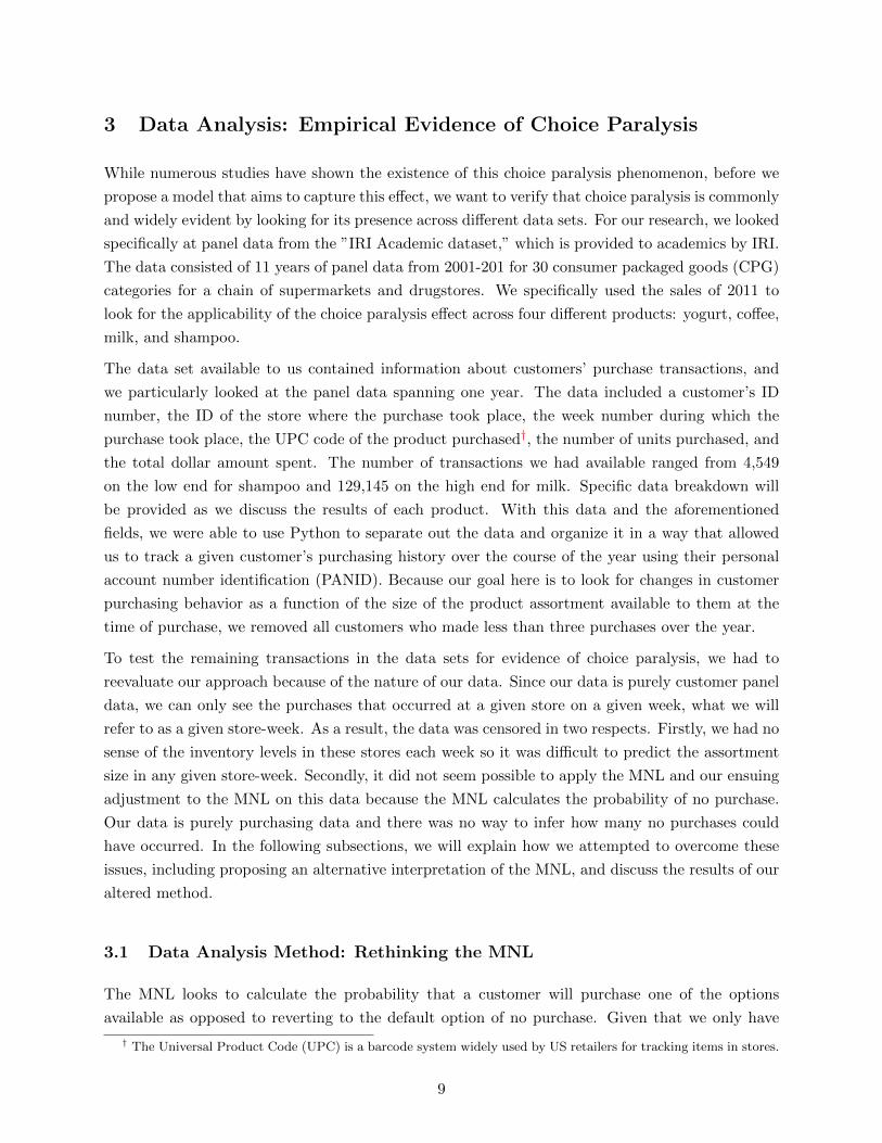
3 Data Analysis: Empirical Evidence of Choice Paralysis

While numerous studies have shown the existence of this choice paralysis phenomenon, before we

propose a model that aims to capture this effect, we want to verify that choice paralysis is commonly

and widely evident by looking for its presence across different data sets. For our research, we looked

specifically at panel data from the ”IRI Academic dataset,” which is provided to academics by IRI.

The data consisted of 11 years of panel data from 2001-201 for 30 consumer packaged goods (CPG)

categories for a chain of supermarkets and drugstores. We specifically used the sales of 2011 to

look for the applicability of the choice paralysis effect across four different products: yogurt, coffee,

milk, and shampoo.

The data set available to us contained information about customers’ purchase transactions, and

we particularly looked at the panel data spanning one year. The data included a customer’s ID

number, the ID of the store where the purchase took place, the week number during which the

purchase took place, the UPC code of the product purchased†, the number of units purchased, and

the total dollar amount spent. The number of transactions we had available ranged from 4,549

on the low end for shampoo and 129,145 on the high end for milk. Specific data breakdown will

be provided as we discuss the results of each product. With this data and the aforementioned

fields, we were able to use Python to separate out the data and organize it in a way that allowed

us to track a given customer’s purchasing history over the course of the year using their personal

account number identification (PANID). Because our goal here is to look for changes in customer

purchasing behavior as a function of the size of the product assortment available to them at the

time of purchase, we removed all customers who made less than three purchases over the year.

To test the remaining transactions in the data sets for evidence of choice paralysis, we had to

reevaluate our approach because of the nature of our data. Since our data is purely customer panel

data, we can only see the purchases that occurred at a given store on a given week, what we will

refer to as a given store-week. As a result, the data was censored in two respects. Firstly, we had no

sense of the inventory levels in these stores each week so it was difficult to predict the assortment

size in any given store-week. Secondly, it did not seem possible to apply the MNL and our ensuing

adjustment to the MNL on this data because the MNL calculates the probability of no purchase.

Our data is purely purchasing data and there was no way to infer how many no purchases could

have occurred. In the following subsections, we will explain how we attempted to overcome these

issues, including proposing an alternative interpretation of the MNL, and discuss the results of our

altered method.

3.1 Data Analysis Method: Rethinking the MNL

The MNL looks to calculate the probability that a customer will purchase one of the options

available as opposed to reverting to the default option of no purchase. Given that we only have

† The Universal Product Code (UPC) is a barcode system widely used by US retailers for tracking items in stores.

9

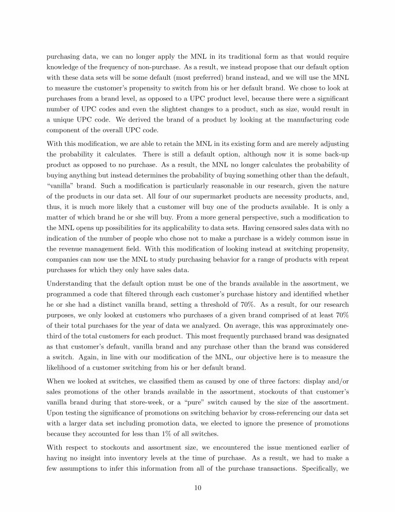
purchasing data, we can no longer apply the MNL in its traditional form as that would require

knowledge of the frequency of non-purchase. As a result, we instead propose that our default option

with these data sets will be some default (most preferred) brand instead, and we will use the MNL

to measure the customer’s propensity to switch from his or her default brand. We chose to look at

purchases from a brand level, as opposed to a UPC product level, because there were a significant

number of UPC codes and even the slightest changes to a product, such as size, would result in

a unique UPC code. We derived the brand of a product by looking at the manufacturing code

component of the overall UPC code.

With this modification, we are able to retain the MNL in its existing form and are merely adjusting

the probability it calculates. There is still a default option, although now it is some back-up

product as opposed to no purchase. As a result, the MNL no longer calculates the probability of

buying anything but instead determines the probability of buying something other than the default,

“vanilla” brand. Such a modification is particularly reasonable in our research, given the nature

of the products in our data set. All four of our supermarket products are necessity products, and,

thus, it is much more likely that a customer will buy one of the products available. It is only a

matter of which brand he or she will buy. From a more general perspective, such a modification to

the MNL opens up possibilities for its applicability to data sets. Having censored sales data with no

indication of the number of people who chose not to make a purchase is a widely common issue in

the revenue management field. With this modification of looking instead at switching propensity,

companies can now use the MNL to study purchasing behavior for a range of products with repeat

purchases for which they only have sales data.

Understanding that the default option must be one of the brands available in the assortment, we

programmed a code that filtered through each customer’s purchase history and identified whether

he or she had a distinct vanilla brand, setting a threshold of 70%. As a result, for our research

purposes, we only looked at customers who purchases of a given brand comprised of at least 70%

of their total purchases for the year of data we analyzed. On average, this was approximately one-

third of the total customers for each product. This most frequently purchased brand was designated

as that customer’s default, vanilla brand and any purchase other than the brand was considered

a switch. Again, in line with our modification of the MNL, our objective here is to measure the

likelihood of a customer switching from his or her default brand.

When we looked at switches, we classified them as caused by one of three factors: display and/or

sales promotions of the other brands available in the assortment, stockouts of that customer’s

vanilla brand during that store-week, or a “pure” switch caused by the size of the assortment.

Upon testing the significance of promotions on switching behavior by cross-referencing our data set

with a larger data set including promotion data, we elected to ignore the presence of promotions

because they accounted for less than 1% of all switches.

With respect to stockouts and assortment size, we encountered the issue mentioned earlier of

having no insight into inventory levels at the time of purchase. As a result, we had to make a

few assumptions to infer this information from all of the purchase transactions. Specifically, we

10

assumed that every brand available in a given store-week was purchased at least once. Under this

assumption, we ran through the entire data set to aggregate all of the brands purchased during a

given store-week and considered that as our assortment. The number of brands in that assortment

was our assortment size, and if a brand was not present in that assortment, we assumed it was out of

stock. If a customer ever purchased another brand other than their default brand and that vanilla

brand was missing from that store-week’s assortment, we considered the switch to be caused by a

stockout. Such stockout switches were isolated out of our data results because we are specifically

looking to understand the effect of the assortment size on a customer’s propensity to switch. All the

aforementioned data issues are common problems for which we used standard measures to address

(see Jagabathula, “Modeling Dynamic Choice Behavior of Customers”).

3.2 Data Analysis Results: Yogurt

Looking first at yogurt, we identified 70 distinct brands and 896 different store-week combinations

in the data set of 121,081 transactions. Of the 3,591 different customer IDs, 38.4% of them had a

vanilla brand they opted to purchase at least 70% of the time. Following the method just discussed,

we want to investigate the relationship between the assortment size and the number of switches

from a vanilla brand at these various assortment sizes. When plotting this relationship, we will

normalize these switches to account for the fact that we would expect to see more switches when

there are more customers. As a result, “fraction of switches” on the y-axis of Figure 1 can be

interpreted as follows: for a given assortment size, the fraction of switches is the fraction of people

who purchased who switched from their default brand. It is calculated as the total number of

switches seen at that assortment size divided by the total number of customers who viewed that

assortment size.

Understanding this distinction, we can see that Figure 1 allows us to see the effect of assortment

size on switching behavior. To make this scatterplot more meaningful, we quantified this effect by

fitting both a linear and quadratic regression line to the data. The results can be seen in the tables

below. By comparing the R2 adjusted values for both lines, we can see that there is a fairly strong

in-sample fit for the quadratic regression line, which has an R2 adjusted of 0.5467.

In addition, both coefficients are statistically significant and we can see that the line indicates a

negative quadratic relationship. Both the plot and the quadratic regression results demonstrate

clear evidence for the choice paralysis phenomenon. We see that, when the assortment size is

really small or really large, customers have a higher likelihood of sticking to their default, vanilla

brand. This is in line with the notion that too little or too much choice can be a bad thing. When

faced with very few options, customers can be fairly confident that their brand is one of the best

available. Similarly, when faced with an excessive number of options, customers may be turned off

by the prospect of evaluating all the options before them and elect to stick to what they know (their

vanilla brand) because it seems like the safest and simplest option. However, when the assortment

size is in the middle range, we see that the propensity to switch increases, suggesting customers

11

Figure 1: Yogurt scatterplot demonstrates strong evidence for a negative quadratic relationship between assort-

ment size and the fraction of switches that occur.

Figure 2: Linear regression and quadratic regression results for yogurt demonstrate strong evidence for a non-

linear relationship between assortment size and propensity to switch.

are more likely to take the time to evaluate the options and try a different brand. Before we

discuss the implications of this result for companies and their decision-making processes, we will

first investigate if this result is consistent across all products.

3.3 Data Analysis Results: Coffee

Within the 24,013 transactions of coffee, there were 96 different brands represented across 769

unique store-weeks. Of the 2,230 customer IDs that purchased coffee over the span of the year,

32.8% of them had a default brand they purchased at least 70% of the time. Plotting the same

relationship as we did with yogurt for coffee in Figure 3, we can see the relationship between the

effect of assortment size on switching for the customers in this data set from the scatterplot as well

12

as the strength of the linear and quadratic regression lines in the tables below.

Figure 3: While not as significant as yogurt, the coffee scatterplot too shows evidence for a non-linear relationship

between assortment size and the fracton of switches.

We notice that, compared to yogurt, coffee’s switching patterns at various assortment sizes are more

spaced out and the negative quadratic relationship is less clear. The R2 adjusted values of both

the linear and quadratic lines further demonstrate this difference. While the quadratic regression is

again a better in-sample fit with an R2 adjusted of 0.2474, this is much weaker than the correlation

we saw with yogurt.

Figure 4: For coffee, linear regression and quadratic regression results show a slightly weaker but still clear

preference for a a non-linear relationship between assortment size and propensity to switch.

Both coefficients, however, are still statistically significant at the 5% level and we still see that the

quadratic relationship is negative. This serves to show that, while the choice paralysis phenomenon

is not as signifcantly and clearly evident with coffee as it is with yogurt, there is still an overall

trend in line with the notion of choice overload and customers still do tend to stick to their vanilla

brand when faced with very small or very large assortment sizes. The results with coffee only

13

serve to reinforce that the strength of this choice paralysis phenomenon will vary from product to

product as customers will be more sensitive to choice with one type of purchase than another.

3.4 Data Analysis Results: Milk

With 129,145 transactions over the course of the year, milk, as expected was the most frequently

purchased product across the four being investigated. There were 92 unique brands of milk in the

data set and these were sold across 1,068 distinct store-weeks. Isolating the customers who qualified

for having a default, vanilla brand, we found that 39.2% of the 4,010 customers purchased the same

brand at least 70% of the time. Figure 5 demonstrates the relationship between assortment size

and fraction of switches for milk.

Looking at the plot, we see that milk varies quite distinctly from both yogurt and coffee in that

a linear regression seems to fit the data just as well as the quadratic. There seems to be a dis-

tinctly positive linear trend in the number of switches as the assortment size increases, with greater

variability in switching behavior as the assortment size becomes very large. Accounting for the

significance of coefficients from the tables below, we see that the linear line’s size coefficient has a

stronger stasticial significance than either of the quadratic’s coefficients. The difference in the R2

adjusted values are also negligible.

Figure 5: The milk scatterplot shows a similar fit for a linear and non-linear relationship for this product. Milk

does not appear to be as effected by this choice paralysis phenomenon.

From a quick analysis of both the plot and regression outputs, we can see that choice paralysis does

not appear to have much of an for milk. In fact, the linear line would suggest that as size increases

even up to the larger end the propensity of a customer to switch from his or her vanilla brand

will also increase. The volatility when the assortment size is greater than 20 is the only reason a

14

Figure 6: Milk showed very minimal difference between the linear and quadratic relationship results. Although

the non-linear relationship appears slightly stronger, this shows that the degree of the choice paralysis effect (and

hence, the effect of assortment size on propensity to switch) varies from product to product.

quadratic regression line still demonstrates a negative relationship on the plot and suggests slight

evidence for the trend we saw both with yogurt and coffee.

In addition to further demonstrating that the applicability of choice paralysis varies from product

to product, the results with milk suggest the products with little differentiation and low brand

identification are much less likely to be prone to switching behavior consistent with choice paralysis.

A product like milk is more or less the same regardless of which brand a customer selects to buy,

and this may have an influence on a customer’s willingness to switch from his or her vanilla brand

and try something new, even when the assortment size is larger.

3.5 Data Analysis Results: Shampoo

Lastly, we can look at the evidence of choice paralysis with a less-frequently purchased product

like shampoo. Our 4,549 shampoo purchase transactions represented 66 distinct brands across 544

different store-weeks. Approximately 30.1% of shampoo’s 575 customers met the 70% vanilla brand

threshold. As you will see with Figure 7, in stark contrast to milk, shampoo shows very strong

evidence of the choice paralysis phenomenon in effect.

Looking at coefficients in the tables below, shampoo was the only product to demonstrate a negative

relationship between assortment size and fraction of switches for both the linear and quadratic

regression lines. However, as we can see from the R2 adjusted values and p-values, a linear line

is not a good fit for this plot. The quadratic regression line, however, performs almost as well as

yogurt with an R2 adjusted value of 0.4850 and strongly significant coefficients. As a result, we can

see that shampoo, like yogurt, shows the strongest evidence of the presence of choice paralysis as

the assortment size changes. Given both of these products are widely known to have stronger brand

distinctions, this observation is in line with the hypothesis for why milk failed to show evidence of

choice paralysis.

15

Figure 7: The shampoo scatterplot shows clear evidence for a negative quadratic relationship between assortment

size and the fraction of switches. Customers were less likely to switch at both small and large assortment sizes.

Figure 8: Shampoo shows a much stronger non-linear relationship between assortment size and propensity to

switch. There appears to be very strong evidence of the choice paralysis phenomenon in this sample.

3.6 Implications of the Results

Generalizing the results of these four products, while strength of the phenomenon varies from

product to product, there is strong empirical evidence that there is non-linear switching behavior

for customers across categories as the assortment size varies. Based on past psychological studies,

one valid explanation for such switching is choice paralysis. While the effect of choice paralysis on

purchasing behavior was the initial interest of this research, empirical discovery of choice paralysis’

impact on customer switching behavior can still have significant business implications. Specifically,

these implications center around inventory management and assortment planning.

Given that we saw this negative quadratic relationship consistently across all the products, although

at varying degrees of strength, we see that switching behavior can play a key role in further

16

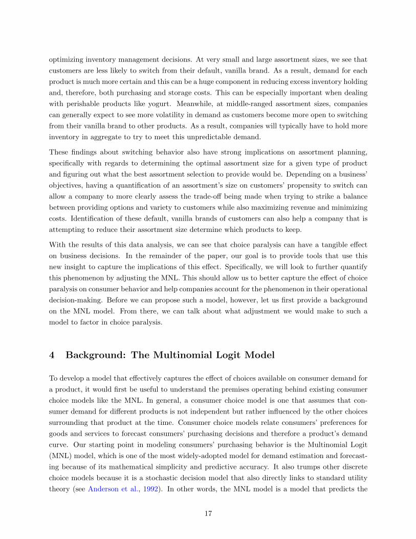
optimizing inventory management decisions. At very small and large assortment sizes, we see that

customers are less likely to switch from their default, vanilla brand. As a result, demand for each

product is much more certain and this can be a huge component in reducing excess inventory holding

and, therefore, both purchasing and storage costs. This can be especially important when dealing

with perishable products like yogurt. Meanwhile, at middle-ranged assortment sizes, companies

can generally expect to see more volatility in demand as customers become more open to switching

from their vanilla brand to other products. As a result, companies will typically have to hold more

inventory in aggregate to try to meet this unpredictable demand.

These findings about switching behavior also have strong implications on assortment planning,

specifically with regards to determining the optimal assortment size for a given type of product

and figuring out what the best assortment selection to provide would be. Depending on a business’

objectives, having a quantification of an assortment’s size on customers’ propensity to switch can

allow a company to more clearly assess the trade-off being made when trying to strike a balance

between providing options and variety to customers while also maximizing revenue and minimizing

costs. Identification of these default, vanilla brands of customers can also help a company that is

attempting to reduce their assortment size determine which products to keep.

With the results of this data analysis, we can see that choice paralysis can have a tangible effect

on business decisions. In the remainder of the paper, our goal is to provide tools that use this

new insight to capture the implications of this effect. Specifically, we will look to further quantify

this phenomenon by adjusting the MNL. This should allow us to better capture the effect of choice

paralysis on consumer behavior and help companies account for the phenomenon in their operational

decision-making. Before we can propose such a model, however, let us first provide a background

on the MNL model. From there, we can talk about what adjustment we would make to such a

model to factor in choice paralysis.

4 Background: The Multinomial Logit Model

To develop a model that effectively captures the effect of choices available on consumer demand for

a product, it would first be useful to understand the premises operating behind existing consumer

choice models like the MNL. In general, a consumer choice model is one that assumes that con-

sumer demand for different products is not independent but rather influenced by the other choices

surrounding that product at the time. Consumer choice models relate consumers’ preferences for

goods and services to forecast consumers’ purchasing decisions and therefore a product’s demand

curve. Our starting point in modeling consumers’ purchasing behavior is the Multinomial Logit

(MNL) model, which is one of the most widely-adopted model for demand estimation and forecast-

ing because of its mathematical simplicity and predictive accuracy. It also trumps other discrete

choice models because it is a stochastic decision model that also directly links to standard utility

theory (see Anderson et al., 1992). In other words, the MNL model is a model that predicts the

17

probability a consumer will select a given product among a set of options by estimating the utility

a consumer will derive from each of the products and assuming the consumer will aim to maximize

his or her utility.

Figure 9 provides a pictorial description of the MNL model. Arriving customers are exposed to an

assortment of products that includes an Offer Set, which we denote by S, and a default option, which

we denote by product ‘0’. In the classical MNL model, this default option is to the no-purchase

option, i.e., the customer walks away without buying anything. In our setting, the default option

corresponds to the consumer’s most preferred (or regular) product and the offer set S includes all

remaining products. We note that since the default option can change from customer to customer

the set S is consumer’s specific.

1

2

k

n

.

.

.

.

.

.

k+1

Offer Set

Arriving Customers

MNL

0 Default Option

Figure 9: The Multinomial Logit Model.

The MNL model provides a probabilistic description of how an arriving consumer who is exposed

to an offer set S –together with the default option– decides which one of the n + 1 products to

select. At the heart of the MNL model is a random utility model that aims to quantify the “utility”

an average consumer assigns to each product. Specifically, the utility that consumer j perceived

from purchase product i is divided in the following two parts:

Uji = Vi + εji, (1)

where Vi is the intrinsic valuation for product i which is a deterministic quantity that represents the

average preferences of the entire population, assuming everyone faces the same characteristics and

constraints. It is essentially the average utility a population would assign to product i. However, the

MNL model recognizes that this is not a very accurate estimation of consumer preferences because

it makes the assumption that all consumers are the identical and have the same utility. Therefore,

18

the second variable within the utility function, εji, is a random “error” component that aims to

capture the idiosyncratic tastes of consumer j as well as the unobserved attributes individual j

may personally assign to product i. As opposed to remaining a deterministic value, utility becomes

a random variable reflecting unobservable taste differences among consumers (see chapter 1 in

Anderson et al., 1992). The MNL model also assumes that these individual perturbations {εji} are

mutually independent across products and among the population of consumers and have a double

exponential (Gumble) distribution:

P(εji ≤ x) = exp (− exp (− [µx+ γ])) ,

where γ ≈ 0.5772 is Euler’s constant and µ is a positive parameter. Although restrictive, the

implications of this particular choice to model the distribution of the random utility components

are remarkably significant in computing the resulting choice probability. Indeed, the probability

that an individual consumer purchases product i is given by

P(Purchase of Product i

)P (i) :=

viv0 +

∑s∈S vs

, where vi := exp(µVi). (2)

The value of vi represents a modified utility associated to the purchase of product i, whose calcula-

tion we just discussed. The probability a consumer purchases any given product i is calculated as

the value or utility of that product vi divided by the sum of the utility of all the products available

plus the value of the default option, v0. The MNL model assumes that a consumer will spend the

time to evaluate all the options available and the probability he or she will purchase a given product

depends on the valuation it gives to that product relative to the value of any other product and

the value of no purchase.

Looking back at the deterministic component of utility, Vi is typically estimated using a regression

model of the observable attributes of a product. That is,

Vi = β0 + β1 xi1 + β2 xi2 + · · ·+ βA xiA,

where each xia (a = 1, . . . , A) variable reflects a different product attribute, such as price, quality,

or volume of the product.

Through this discussion of the MNL model, we see that it effectively incorporates an element of

consumer preferences and utility in its forecasting of a consumer’s likelihood to purchase a given

product. In addition, it incorporates some element of consumer heterogeneity with the error term

in the utility calculation to account for inherent preferences of individual consumers that we cannot

directly capture. However, the MNL model still has many limitations. In particular, the MNL is

still confined to situations where the “independence from irrelevant alternatives property” holds

(see Anderson et al., 1992). In addition, the MNL model assumes that the consumer evaluates

every product available before making a purchasing decision. Given this assumption, the MNL

perpetuates the idea that more is better. The more options you provide, the more likely it is that

19

every customer will find an ideal option suited for him or her. In particular, the probability that a

consumer switches from her default option and buys something from the offer set S increases with

the cardinality of S.

However, given the psychological research we have discussed on choice, this may not be a viable

assumption. Rather, it is more likely that customers will make a decision prior to evaluating all

the options or will find the option of no purchase the most attractive given the transaction and

mental costs of finding the best option are too taxing. As customers, we have a limited amount

of time or energy to spend on making a purchase decision. We will refer to this limited capacity

as a customer’s “patience” or “cognitive budget.” In the following section, we hope to take the

existing MNL model and more precisely capture the effect of choice paralysis within it, adjusting

the MNL to measure switching behavior as proposed earlier. Specifically, we will be looking to

better quantify the effect of the number of options available for a consumer to choose from on a

consumer’s probability of switching from their default option v0.

5 The Multinomial Logit Model with Choice Paralysis (MNL-CP)

To effectively modify the MNL to capture choice paralysis in its demand estimation, we aim to in-

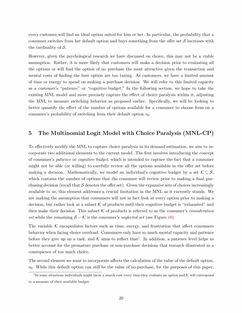
corporate two additional elements to the current model. The first involves introducing the concept

of consumer’s patience or cognitive budget, which is intended to capture the fact that a consumer

might not be able (or willing) to carefully review all the options available in the offer set before

making a decision. Mathematically, we model an individual’s cognitive budget by a set K ⊆ S,

which contains the number of options that the consumer will review prior to making a final pur-

chasing decision (recall that S denotes the offer set). Given the expansive sets of choices increasingly

available to us, this element addresses a crucial limitation in the MNL as it currently stands. We

are making the assumption that consumers will not in fact look at every option prior to making a

decision, but rather look at a subset K of products until their cognitive budget is “exhausted” and

then make their decision. This subset K of products is referred to as the consumer’s consideration

set while the remaining S − K is the consumer’s neglected set (see Figure 10).

The variable K encapsulates factors such as time, energy, and frustration that affect consumers

behavior when facing choice overload. Consumers only have so much mental capacity and patience

before they give up on a task, and K aims to reflect that‡. In addition, a patience level helps us

better account for the premature purchase or non-purchase decisions that research illustrated as a

consequence of too much choice.

The second element we want to incorporate affects the calculation of the value of the default option,

v0. While this default option can still be the value of no-purchase, for the purposes of this paper,

‡In some situations individuals might incur a search cost every time they evaluate an option and K will correspond

to a measure of their available budget.

20

.

.

.

.

.

.

Offer Set

Consideration Set

Neglected Set

Arriving Customers

0

MNL-CP

Default Option

n

k+1

1

2

k

Figure 10: The Multinomial Logit Mode with Choice Paralysis.

we will treat it as the value of sticking to your go-to, vanilla option. When we have S options

available to us but only have a patience level of K, where K ( S, we think it is fair to assume

that the number of options we never end up viewing, S − K, will affect the value we place on our

default option. As the size of the set S − K of un-viewed options increases, the probability that

a consumer will revert to her default option should also increase. This relates to the idea that a

consumer will more likely feel like she is making a premature or uninformed selection when she has

viewed only a small subset of the entire sample. To capture this remorse, we modify the utility

that consumer j gets by purchasing product i by penalizing her intrinsic valuation Vi with a factor

that is proportional to the number of products in her neglected set. To be more precise, we rewrite

consumer’s j utility Uji in equation (1) as follows:

Uji = Vi − f(S − K) + εji, i ∈ K (3)

where f(·) is a non-negative increasing set function that captures consumer’s j disutility. On the

other hand, consumer’s j utility for the default option remains unchanged, that is,

Uj0 := Uj0 = V0 + εj0.

As in the traditional MNL model, we assume the disturbances {εji} to be iid with a Gumbel

distribution. As a result, the probability that consumer j purchases product i ∈ K conditional on

consumer j having the consideration set K is equal to

P (i|K) :=vi

v0 exp(µ f(S − K)) +∑

s∈K vsi ∈ K, (4)

where vi := exp(µVi). Similarly, the probability that the consumer chooses the default option is

21

P (0|K) :=v0 exp(µ f(n−K))

v0 exp(µ f(S − K)) +∑

s∈K vs.

From the seller’s perspective, the set K is unknown and in order to compute the purchasing proba-

bilities he must compute unconditional probabilities. For this, he needs to estimate the probability

distribution of K among the population of consumers and compute the expected value over K of

the probabilities in (4), that is,

P (i) = E[

viv0 exp(µ f(S − K)) +

∑s∈K vs

]and P (0) := E

[v0 exp(µ f(S − K))

v0 exp(µ f(S − K)) +∑

s∈K vs

].

The set function f(·) becomes an additional input –together with the value of the {vi}’s– that needs

to be estimated and calibrated from data. This can prove to be a difficult task if the cardinality of

the offer set S is large as one must estimate 2n values, where n = ‖S‖ is the cardinality of the offer

set. One possible approach to tackle this problem is to use a a parametric representation of f(·).

In what follows, we describe an alternative approach which leads to a simple representation of f(·).This refinement is a direct extension of the MNL model and we will refer to it as the multinomial

logic model with consumer paralysis (MNL-CP). The MNL-CP model is built upon the idea that

a consumer with a cognitive budget K will react to the fact that she has incomplete information

by randomizing her purchasing decision. To describe this purchasing process, consider a consumer

with a cognitive budget K ⊆ S. The information available to her is the values of the intrinsic

valuations {Vi : i ∈ S ∪ {0}} as well as the value of her idiosyncratic perturbations for the

products in her consideration set {εi : i ∈ K ∪ {0}}. On the other hand, the consumer does not

the values of these perturbations for the products in her neglected set {εi : i ∈ S − K}. With

this information, she computes the utility of the products in her consideration set {Ui = Vi + εi :

i ∈ K}, the maximum utility U∗K := max{Ui : i ∈ K} and corresponding best alternative product

i∗K := argmax{Ui : i ∈ K}. Knowing the value of U∗K, the consumer randomizes her purchasing

decision and buys the product i∗K instead of selecting her default option with probability

P(U∗K ≥ U0 ∨max{Vi + εi : i ∈ S − K}

).

In other words, the consumer evaluates the utility of her best alternative product in K, estimates

the likelihood that this product dominates every other one in the offer set, and buys it with a

probability that is consistent with her estimates. Under this purchasing behavior, the probabilities

in (4) are given by

P (0|K) :=v0∑

s∈S−K vs

v0 +∑

s∈S vsand P (i|K) :=

viv0 +

∑s∈S vs

i ∈ K. (5)

From this, it follows that the penalty function f(·) associated to the MNL-CP model is given by

f(K) =1

µln

(1 +

∑i∈K

eµ (Vi−V0)

).

22

5.1 MNL-CP Model with Homogeneous Products

In this section we specialize the MNL-CP model to the case of homogeneous products. That is, we

assume that all products are nearly identical and hold the same valuation by customers, namely

that vi = v for some constant v and for every product i ∈ S§. Taking this into account, we can now

factor in the concept of a cognitive budget. Given that K is the number of products the consumer

is willing or able to review before making a purchase decision, we expect that a lower number

of options will induce a greater chance of purchase. For example, when the number of products

available is 5 or 10, it would be reasonable to believe that the consumer will consider all the

available options and make a selection accordingly. However, as the selection of products increases

into the 20s, 50s, and even 100s in the case of online channels, it is much more reasonable to believe

that people have time, energy, and/or motivation considerations that will limit their capacity and

interest to evaluate all the available products. We saw evidence of such a trend potentially at play

when the assortment sizes were large for the supermarket data.

In what follows we let ‖S‖ = n be the cardinality of the offer set. There are two scenarios that can

arise when factoring in this patience constraint of K products. In some instances, n < K, in which

case the model would function like a traditional MNL model where the customer evaluates all n

products and makes a purchasing decision accordingly. Remember here that v0 is the value of the

default option and vi = v is the value assigned to product i in this homogeneous case. Therefore,

the probability of switching to any one of these homogenous products in the offer set would be as

follows:

P(Switching | K ≥ n

)=

n v

v0 + n v.

The numerator of this formula includes the valuations of each of the possible outcomes we would

want. In this situation, that would be the sum of the valuation of all n products: v1 +v2 + · · ·+vn.

However, given this is the homogeneous case and v = vi, this simplifies to v n. The denominator of

this formula is a summation of all the possible outcomes, which includes the valuation of each of

the n products as well as the valuation of the default option, v0. In this way, this formula calculates

the probability that a consumer will choose one of these homogenous products.

On the other hand, when n > K the concept of impatience comes into play. The consumer will

no longer evaluate all n products; instead, the consumer will only evaluate K products and then

make a decision. As a result, n−K products will remain unevaluated prior to making a purchase

decision, and hence, the probability of switching will be:

P(Switching | K < n

)=

K vv0 + n v

.

In contrast to the n ≤ K scenario, we see that the numerator in this instance is instead K v. This

reflects that the consumer only viewed K options, and therefore, the probability of switching is

§Basic or staple product categories (i.e., mature products with regular demand patterns) such as most grocery

products (e.g., coffee, detergent, etc.) are more likely to satisfy this condition.

23

limited to the probability of switching to one of those K items. As a result, this naturally reduces

the probability of switching because there are n − K options that were not viewed but whose

valuation remains a component of the denominator. To better understand this, we could also have

written the denominator as v0+vK, where v0 := v0+(n−K) v is a modified utility of non-purchase

that incorporates the utility of the products that were not viewed. Hence, the n − K component

reflects the added valuation to sticking to your vanilla option, which is created by there being too

many options for a consumer to evaluate.

From the seller’s perspective –who is trying to incorporate this limited cognitive budget into her

models– the value of K is not known and moreover it varies from customer to customer. Therefore,

it seems reasonable to treat K as a random variable with a probability mass function {pk : k =

1, 2, . . . }. Factoring in this variation in the value of K, the probability of switching can then be

further developed to as follows:

P(Switching

)=

n∑k=1

(k v

v0 + n v

)pk +

∞∑k=n+1

(n v

v0 + n v

)pk =

E[min{K, n}].v0 + n

, (6)

where v0 := v0/v is the relative (or normalized) default option utility.

It follows that an optimal assortment size can obtain solving the optimization problem

n∗ = argmaxn≥1

{E[min{K, n}]

v0 + n

}. (7)

The following are some general properties of n∗ and the probability of switching.

Proposition 1

a) The probability of switching in equation (6) is a unimodal function of n. As a result, n∗

satisfies

v0 P(K ≥ n∗)−n∗−1∑k=1

k pk > 0 ≥ v0 P(K ≥ n∗ + 1)−n∗∑k=1

k pk.

b) If

v0 ≤p1

1− p1then n∗ = 1 and P

(Switching

)=

1

v0 + 1.

c) Suppose the distribution of K is bounded, that is, there exists a positive integer N such that

pN > 0 and pk = 0 for all k ≥ N + 1. If

v0 ≥E[K]

pN−N then n∗ = N and P

(Switching

)=

E[K]

v0 +N.

The solve equation (7) we need to specify the probability distribution for the random variable K.

Here are some concrete examples.

24

Example 1 (Uniform Distribution) Suppose that k is uniformly distributed in {1, 2, . . . , N} for some

fixed integer N , that is, pk = 1/N for k = 1, . . . , N and pk = 0 otherwise. It follows that for n ≤ N

P(Switching

)=

2Nn− n2 + n

2N (v0 + n)and n∗ = argmax

n≥1

{2Nn− n2 + n

v0 + n

}.

Using a continuous approximation (i.e., relaxing the integrability constraint by letting n be a continuous

variable) we get

n∗ ≈√v20 + (2N + 1) v0 − v0 and P

(Switching

)≈ 1− 2n∗ − 1

2N.

As expected, n∗ is increasing in v0 and n∗ ↑ N as v0 →∞.

Example 2 (Geometric Distribution) Suppose that k follows a geometric distribution with parameter

ρ, that is, pk = (1− ρ) ρk−1 then

P(Switching

)=

(1− ρn)

(1− ρ) (v0 + n)and n∗ = argmax

n≥1

{1− ρn

v0 + n

}.

Similar to the previous example, using a continuous approximation let y∗ be the unique non-positive

root of the equation: ey [1− y − v0 ln(ρ)] = 1. Then,

n∗ ≈ y∗

ln(ρ)and P

(Switching

)≈ − ln(ρ)

1− ρρn∗.

6 Application and Key Takeaways

Developing a model that incorporates choice paralysis in the MNL model can provide companies

with the necessary tools to help capture the implications of choice paralysis. Specifically, it will allow

both retailers and vendors to now more precisely quantify the effect of assortment size on customers’

propensity to switch, specifically by estimating the distribution of the random variable k for the

selected product. The cognitive budget level k will vary from product to product. Customers

will likely have a larger cognitive budget and more patience for less frequently purchased and

more expensive products, for example. By calibrating the k to the data set under consideration,

companies can determine the optimal assortment size for their business objectives.

From a retailer’s perspective, the implications of choice paralysis are primarily operational. Our

data analysis results helped quantify the strength of this effect on a given product, and our model

will allow retailers to address the effect size has on their customers’ behavior. Specifically, a

retailer who is looking to entice customers to try new products would actually want to promote

switching behavior and may seek to maximize the propensity to switch. Given this objective, the

MNL-CP model can be used to determine the optimal assortment size to meet this objective. In

25

contrast, a retailer who is looking to reduce demand uncertainty and limit inventory requirements

while still providing customers with a variety of options can use the MNL to determine customers’

assortment size sensitivity. The MNL provides these retailers with a better understanding of how

their assortment size decisions will affect their aggregate inventory levels and, translating it further,

their revenue.

From a vendor’s perspective, understanding this choice paralysis behavior and the effect of as-

sortment size may be useful in determining how many products to manufacture and provide. A

vendor who is looking to entice switching behavior and potentially convert customers to their brand

could use information about the retailers’ inventory variety and assortment size decisions to better

estimate the revenue potential of having their brand represented in the retail outlet.

Beyond these group-specific applications, the key takeaways from this research are really three-fold.

Firstly, both through the empirical data analysis and development of the MNL-CP model, we have

managed to more precisely quantify the choice paralysis effect so it can be accounted for in future

decision-making. Such a quantification allows companies to determine the magnitude of choice

paralysis’ impact on their customers’ purchasing behavior for a given product. Secondly, we have

proposed an extension of the MNL model’s use so that it can be applied even on censored purchasing

data. We demonstrated that the MNL model as it is popularly known today can be equally used

to measure the propensity of a customer to switch from a default product or brand. The v0 can

be generalized to refer to as some default option. That default option can either be the traditional

no-purchase option or, in situations in which customers are highly likely to make some sort of

purchase, it can be the purchase of some vanilla brand. Lastly, our research has provided insight

into how the assortment size can effect demand volatility with respect to inventory management. It

provides operational decision makers with a key factor to consider when making their assortment

planning and inventory purchasing decisions so that they can most effectively minimize costs while

remaining in line with their companies’ overall business objectives.

7 Further Research

There are a number of next steps that can be taken to further the research in the realm of choice

paralysis and its effect on business decision making. From a data analysis perspective, research

into what features or characteristics make a product more prone to the choice paralysis effect can

be incredibly instructive. Such insight can help companies determine how seriously they need to

be considering such a phenomenon in their decision making. It would be important to consider

this not only within similar-class goods, such as the varying strengths of choice paralysis across the

supermarket products investigated in this paper, but also in other classes of goods that are perhaps

larger purchases or not as urgently or frequently purchased.

As a next step to the modeling ideas proposed here, considering how this notion of choice paralysis

can be factored in when dealing with heterogeneous products that do not hold the same valuation vi

26

would be instrumental in furthering the ideas laid out in the MNL-CP and widening its applicability.

As the proposed model currently stands, the MNL-CP can only be applied to homogeneous sets of

products.

Lastly, looking back at the MNL as it was originally intended, measuring the impact of choice

paralysis in fueling no purchase should be considered in the realm of online channels, particularly

as the online medium has experienced the greatest explosion of options. Web traffic data would

also be less censored, overcoming the barrier of most in-store data’s inability to track the frequency

of non-purchase. By quantifying choice paralysis in the online realm, research can fuel discussion

on how companies can better present products so that customers do not get overwhelmed by the

options available to them while still allowing companies to provide the variety that they know

customers seek.

References

Anderson, S., A. de Palma, J.F. Thisse. 1992. Discrete Choice Theory of Product Differentiation.

The MIT Press, Cambridge, Massachusetts. 17, 19

Cutrone, C. 2013. Cutting down on choice is the best way to make better decisions. Business

Insider . 7

Iyengar, S. 2010. The Art of Choosing . Twelve, Grand Central Publishing, New York. 7, 8

Miller, G. 1956. The magical number seven, plus or minus two: Some limits on our capacity for

processing information. The Psychological Review 63(2) 81–97. 8

Schwartz, B. 2004. Paradox of Choice. HarperCollins Publishers, Inc. 7, 8

Worth, T. 2009. Too many choices can tax the brain, research shows. Los Angeles Times . 8

27