The Implicit Convex FeasibilityProblem and Its Application to

Adaptive Image Denoising

Yair Censor1, Aviv Gibali2, Frank Lenzen3 and Christoph Schnorr3

1Department of Mathematics, University of Haifa,Mt. Carmel, 3498838 Haifa, Israel

2Department of Mathematics, ORT Braude College,2161002 Karmiel, Israel

3 Heidelberg Collaboratory for Image Processing,Mathematikon, INF 205, University of Heidelberg,

69120 Heidelberg, Germany

March 20, 2016. Revised: June 14, 2016.

Abstract

The implicit convex feasibility problem attempts to find a pointin the intersection of a finite family of convex sets, some of whichare not explicitly determined but may vary. We develop simultaneousand sequential projection methods capable of handling such problemsand demonstrate their applicability to image denoising in a specificmedical imaging situation. By allowing the variable sets to undergoscaling, shifting and rotation, this work generalizes previous resultswherein the implicit convex feasibility problem was used for coopera-tive wireless sensor network positioning where sets are balls and theircenters were implicit.

Keywords: Implicit convex feasibility · split feasibility · projec-tion methods · variable sets · proximity function · image denoising

1

1 Introduction

In this paper we are concerned with the following “implicit convex feasibilityproblem” (ICFP). Given set-valued mappings Cs : Rn → 2Rn

, s = 1, 2, . . . , S,with closed and convex value sets, the ICFP is,

Find a point x∗ ∈ ∩Ss=1Cs(x∗). (1.1)

We call the sets Cs(x) “variable sets” for obvious reasons and include“implicit” in this problem name because the sets defining it are not givenexplicitly ahead of time. The problem is inspired by the work of Gholamiet al. [21] on solving the cooperative wireless sensor network positioningproblem in R2 (Rn). There, the sets Cs(x) are circles (balls) with varyingcenters. A special instance of the ICFP is obtained by taking fixed setsCs(x) ≡ Cs, for all x ∈ Rn, and all s = 1, 2, . . . , S, yielding the well-known,see, e.g., [3], “convex feasibility problem” (CFP) which is,

Find a point x∗ ∈ ∩Ss=1Cs. (1.2)

The CFP formalism is at the core of the modeling of many inverse prob-lems in various areas of mathematics and the physical sciences. This prob-lem has been widely explored and researched in the last decades, see, e.g.,[10, Section 1.3], and many iterative methods where proposed, in particularprojection methods, see, e.g., [11]. These are iterative algorithms that useprojections onto sets, relying on the principle that when a family of sets ispresent, then projections onto the given individual sets are easier to performthan projections onto other sets (intersections, image sets under some trans-formation, etc.) that are derived from the given individual sets.

Gholami et al. in [21] introduced the implicit convex feasibility problem(ICFP) in Rd (d = 2 or d = 3) into their study of the wireless sensor net-work (WSN) positioning problem. In their reformulation the variable setsare circles or balls whose centers represent the sensors’ locations and theirbroadcasting range is represented as the radii. Some of these centers areknown a priori while the rest are unknown and need to be determined. TheWSN positioning problem is to find a point, in an appropriate product space,which represents the circles or balls centers. The precise relationship betweenthe WSN problem and the ICFP can be found in [21, Section B]. For moredetails and other examples of geometric positioning problems, see [20, 22].

2

We focus on the ICFP in Rn and present projection methods for its solu-tion. This expands and generalizes the special case treated in Gholami et al.[21]. Moreover, we demonstrate the applicability of our approach to the taskof image denoising, where we impose constraints on the image intensity atevery image pixel. Because the constraint sets depend on the unknown vari-ables to be determined, the method is able to adapt to the image contents.This application demonstrates the usefulness of the ICFP approach to imageprocessing.

The paper is structured as follows. In Section 2 we show how to calculateprojections onto variable sets. In Section 3 we present two projection typealgorithmic schemes for solving the ICFP, sequential and simultaneous, alongwith their convergence proofs. In Section 4 we present the ICFP applicationto image denoising together with numerical visualization of the performanceof the methods. Finally, in Section 5 we discuss further research directionsand propose a further generalization of the ICFP.

2 Projections onto variable convex sets

We begin by recalling the split convex feasibility problem (SCFP) and theconstrained multiple-set split convex feasibility problem (CMSSCFP) thatwill be useful to our subsequent analysis.

Problem 2.1 Censor and Elfving [13]. Given nonempty, closed and convexsets C ⊆ Rn, Q ⊆ Rm and a linear operator T : Rn → Rm, the Split

Convex Feasibility Problem (SCFP) is:

Find a point x∗ ∈ C such that T (x∗) ∈ Q. (2.1)

Another related more general problem is the following.

Problem 2.2 Masad and Reich [31]. Let r, p ∈ N and Ωs, 1 ≤ s ≤ S, andQr, 1 ≤ r ≤ R, be nonempty, closed and convex subsets of Rn and Rm, re-spectively. Given linear operators Tr : Rn → Rm, 1 ≤ r ≤ R and anothernonempty, closed and convex Γ ⊆ Rn, the Constrained Multiple-Set

Split Convex Feasibility Problem (CMSSCFP) is:

Find a point x∗ ∈ Γ such that

x∗ ∈ ∩Ss=1Ωs and Tr(x∗) ∈ Qr for each r = 1, 2, . . . , R. (2.2)

3

If Tr ≡ T for all r = 1, 2, . . . , R, then we obtain a multiple-set split convexfeasibility problem (MSSCFP) [14].

A prototype for the above SCFP and MSSCFP is the Split InverseProblem (SIP) presented in [8, 15] and given next.

Problem 2.3 Given two vector spaces X and Y and a linear operator A :X → Y , we look at two inverse problems. One, denoted by IP1, is formu-lated in X and the second, denoted by IP2, is formulated in Y . The Split

Inverse Problem (SIP) is:

Find a point x∗ ∈ X that solves IP1such that y∗ = Ax∗solves IP2. (2.3)

In [8, 15] different choices for IP1 and IP2 are proposed, such as variationalinequalities and minimization problems. The latter enable, for example,to obtain a least-intensity feasible solution in intensity-modulated radiationtherapy (IMRT) treatment planning as in [39]. In [23] we further explore andextend this modeling technique to include non-linear mappings between thetwo spaces X and Y .

Let C ⊆ Rn be a nonempty, closed and convex set. For each point x ∈ Rn,there exists a unique nearest point in C, denoted by PC(x), i.e.,

‖x− PC (x)‖ ≤ ‖x− y‖ , for all y ∈ C. (2.4)

The mapping PC : Rn → C is the metric projection of Rn onto C. It iswell-known that PC is a nonexpansive mapping of Rn onto C, i.e.,

‖PC (x)− PC (y)‖ ≤ ‖x− y‖ , for all x, y ∈ Rn. (2.5)

The metric projection PC is characterized by the following two properties:

PC(x) ∈ C (2.6)

and〈x− PC (x) , y − PC (x)〉 ≤ 0, for all x ∈ Rn, y ∈ C. (2.7)

If C is a hyperplane, then (2.7) becomes an equality, [24]. We are dealingwith variable convex sets that can be described by set-valued mappings.

Definition 2.4 For a set-valued mapping C : Rn → 2Rn, we call the sets

C(x) ⊆ Rn, defined below, “variable sets”. Let Ω ⊆ Rn be a given set, calledin the sequel a “core set”.

4

(i) Given an operator µ : Rn → Rn, the variable sets C(x) := Ω +µ(x) =y + µ(x) | y ∈ Ω , for x ∈ Rn, are obtained from shifting Ω by the vectorsµ(x).

(ii) Given an x ∈ Rn let U[x] : Rn → Rn be a linear bounded operator.The variable sets C(x) := U[x](Ω) =

U[x]y | y ∈ Ω

are the U[x] images of Ω.

(iii) Given a function f : Rn → R+, the variable sets C(x) := f(x)Ω =f(x)y | y ∈ Ω , for x ∈ Rn, are obtained from scaling Ω uniformly by f(x).This can be re-written as in (ii) with U[x] = f(x)I, where I is the identitymatrix.

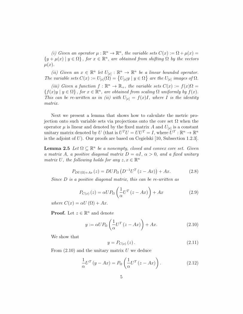
Next we present a lemma that shows how to calculate the metric pro-jection onto such variable sets via projections onto the core set Ω when theoperator µ is linear and denoted by the fixed matrix A and U[x] is a constantunitary matrix denoted by U (that is UTU = UUT = I, where UT : Rn → Rn

is the adjoint of U). Our proofs are based on Cegielski [10, Subsection 1.2.3].

Lemma 2.5 Let Ω ⊆ Rn be a nonempty, closed and convex core set. Givena matrix A, a positive diagonal matrix D = αI, α > 0, and a fixed unitarymatrix U , the following holds for any z, x ∈ Rn

PDU(Ω)+Ax (z) = DUPΩ

(D−1UT (z − Ax)

)+ Ax. (2.8)

Since D is a positive diagonal matrix, this can be re-written as

PC(x) (z) = αUPΩ

(1

αUT (z − Ax)

)+ Ax (2.9)

where C(x) = αU (Ω) + Ax.

Proof. Let z ∈ Rn and denote

y := αUPΩ

(1

αUT (z − Ax)

)+ Ax. (2.10)

We show thaty = PC(x) (z) . (2.11)

From (2.10) and the unitary matrix U we deduce

1

αUT (y − Ax) = PΩ

(1

αUT (z − Ax)

). (2.12)

5

By the characterization of the metric projection onto Ω (2.7) we have

⟨1

αUT (z − Ax)− 1

αUT (y − Ax) , w − 1

αUT (y − Ax)

⟩≤ 0, for all w ∈ Ω.

(2.13)Since α > 0 and U is unitary, we get

〈z − y, αUw + Ax− y〉 ≤ 0, for all w ∈ Ω. (2.14)

Denoting v := αUw + Ax, since w ∈ Ω we get v ∈ αU (Ω) + Ax = C(x),the

〈z − y, v − y〉 ≤ 0, for all v ∈ C(x), (2.15)

and again by the characterization of the metric projection onto C(x) (2.7)and by (2.10) y = PC(x) (z) which completes the proof.

Figure 1: Illustration of Lemma 2.5 with D,U = I

6

Figure 2: Illustration of Lemma 2.5 with D = I and A = 0

Two special cases of Lemma 2.5 are illustrated. In Figure 1 we use D,U =I so that PΩ+Ax (z) = PΩ (z − Ax) + Ax, meaning that the set Ω is shiftedby the point Ax to Ω + Ax. In Figure 2 we use D = I and A = 0 so thatPU(Ω) (z) = UPΩ

(UT z

), meaning that the set Ω is rotated by the unitary

matrix U to U (Ω).

7

3 The algorithms

The following definitions will be used.

Definition 3.1 A sequence σkk∈N of real positive numbers is called a steering

sequence if it satisfies all the following conditions: (i) limk→∞ σk = 0; (ii)

limk→∞σk+1σk = 1; and (iii)

∑∞k=0 σk = +∞. Let β be a positive integer. If

condition (ii) is replaced by

limk→∞

σkβ+j

σkβ= 1, for all 1 ≤ j ≤ β − 1, (3.1)

and (i) and (iii) remain unchanged then the sequence is called an β-steeringsequence.

Definition 3.2 A sequence i(k)k∈N of indices is called a cyclic control

sequence over the index set 1, 2, . . . , S if

i(k) = kmodS, for k ≥ 0. (3.2)

Problem 3.3 The Implicit Convex Feasibility Problem. Given set-valued mappings Cs : Rn → 2Rn

, s = 1, 2, . . . , S, with closed convex valuesCs(x), the Implicit Convex Feasibility Problem (ICFP) is

Find a point x∗ ∈ ∩Ss=1Cs(x∗). (3.3)

One way of handling this problem is to reformulate it as the unconstrainedminimization

minimize Gicfp(x)subject to x ∈ Rn,

(3.4)

where

Gicfp(x) :=1

2

S∑s=1

‖x− PCs(x)(x)‖2 (3.5)

in which PCs(x) is the metric projection operator onto the sets Cs(x).Following the works of Censor et al. [12] and Gholami et al. [21] we

present two algorithmic schemes, simultaneous and sequential, for solvingthe ICFP of Problem 3.3. For s = 1, 2, . . . , S, let Ωs be nonempty, closedand convex core sets in Rn, As ∈ Rn×n are matrices, Us ∈ Rn×n are unitary

8

matrices, and αs > 0. Then the variable sets defined in Definition 2.4 takethe form

Cs(x) = αsUs (Ωs) + Asx, (3.6)

and we assume that the projection PΩs are at hand or can be easily calculated.

Algorithm 3.4 The Simultaneous AlgorithmPreliminary calculations: For s = 1, 2, . . . , S, calculate the matrices

Ks :=1

αsUTs (I − As) (3.7)

and use matrix 2-norms to calculate the constant

Licfp =S∑s=1

‖I − As‖22 . (3.8)

Initialization: Select an arbitrary starting point x0 ∈ Rn and set k = 0.

Iterative step: Given the current iterate xk, calculate the next iterateby

xk+1 = xk − γkS∑s=1

α2sK

Ts (I − PΩs)

(Ksx

k), (3.9)

where γk ∈ (0, 2/Licfp) for all k ≥ 0.

Stopping rule: If xk+1 = xk (or, alternatively, if ‖xk+1 − xk‖ is smallenough) then stop. Otherwise, set k ← (k + 1) and go back to the beginningof the iterative step.

Algorithm 3.5 The Sequential AlgorithmPreliminary calculation: For s = 1, 2, . . . , S, calculate the matrices

Ks :=1

αsUTs (I − As) . (3.10)

Initialization: Select an arbitrary starting point x0 ∈ Rn and set k = 0.

Iterative step: Given the current iterate xk, calculate the next iterateby

xk+1 = xk − σkα2i(k)K

Ti(k)

(I − PΩi(k)

) (Ki(k)x

k), (3.11)

9

where σkk∈N and i(k)k∈N are a β-steering and a cyclic control sequences,respectively.

Stopping rule: If xk+1 = xk (or, alternatively, if ‖xk+1 − xk‖ is smallenough) then stop. Otherwise, set k ← (k + 1) and go back to the beginningof the iterative step.

3.1 Convergence

For the mappings Cs(·) of (3.6) we get, from Lemma 2.5, a simplified formof the proximity function Gicfp in (3.5),

Gicfp(x) =1

2

S∑s=1

∥∥∥∥x− (αsUsPΩs

(1

αsUTs (x− Asx)

)+ Asx

)∥∥∥∥2

=1

2

S∑s=1

∥∥∥∥αsUs (I − PΩs)

(1

αsUTs (I − As)x

)∥∥∥∥2

=1

2

S∑s=1

α2s

∥∥∥∥(I − PΩs)

(1

αsUTs (I − As)x

)∥∥∥∥2

=1

2

S∑s=1

α2s ‖(I − PΩs) (Ksx)‖2 , (3.12)

where Ks is as in (3.7).

In order to prove convergence of Algorithm 3.4 we need to show thatthe function Gicfp is convex, continuously differentiable and that its gradi-ent is Lipschitz continuous (see [21, Proposition 4]). For the convergence ofAlgorithm 3.5 it is sufficient to show only convexity and continuous differen-tiability of Gicfp, see [12, Theorem 6]. In both cases our analysis relies onthe classical theorems of Baillon and Haddad [2] and of Dolidze [18].

Proposition 3.6 The function Gicfp of (3.12) is (1) convex, (2) continu-ously differentiable, and (3) its gradient is Lipschitz continuous.

Proof. Recall that the SCFP (2.1) can also be formulated as the mini-mization problem

minimize Gscfp(x) := 12‖Tx− PQ (Tx)‖2

subject to x ∈ C, (3.13)

10

see, e.g., [7], and, moreover, for the CMSSCFP (2.2) we haveminimize Gcmsscfp(x) := 1

2

∑Ss=1 ‖x− PΩs (x)‖2 + 1

2

∑Rr=1 ‖Trx− PQr (Trx)‖2

subject to x ∈ Γ,(3.14)

see [31]. Since our proximity function Gicfp (3.12) shares some commonfeatures with the above Gscfp and Gcmsscfp functions, we follow the lines of[31] and [21, Theorem 2] to prove the proposition.

(1) The convexity of Gicfp (3.12) is obvious, see, for example [31, Lemma2].

(2) Since∇Gscfp(x) = T T (I − PQ) (Tx) (3.15)

(T T is the transpose of T ) we deduce that

∇Gicfp(x) =S∑s=1

α2sK

Ts (I − PΩs) (Ksx) , (3.16)

where KTs = (1/αs)

(I − ATs

)Us, and continuous differentiability follows.

(3) To show that ∇Gicfp is Lipschitz continuous, that is

‖∇Gicfp(x)−∇Gicfp(y)‖ ≤ Licfp ‖x− y‖ , for all x, y ∈ Rn, (3.17)

we write

∇Gicfp(x)−∇Gicfp(y) =S∑s=1

α2sK

Ts (I − PΩs) (Ksx)−

S∑s=1

α2sK

Ts (I − PΩs) (Ksy)

=S∑s=1

α2sK

Ts (I − PΩs) (Ksx−Ksy) . (3.18)

The firm-nonexpansivity of the projection operator, see, e.g., [10, Definion2.2.1] along with the triangle and the Cauchy–Schwarz inequalities imply

‖∇Gicfp(x)−∇Gicfp(y)‖ =

∥∥∥∥∥S∑s=1

α2sK

Ts (I − PΩs) (Ksx−Ksy)

∥∥∥∥∥≤

S∑s=1

α2s

∥∥KTs

∥∥2‖Ks‖2 ‖x− y‖

=S∑s=1

α2s

∥∥KTs Ks

∥∥2‖x− y‖ . (3.19)

11

Calculating

KTs Ks =

1

α2s

(I − ATs

)UsU

Ts (I − As)

=1

α2s

(I − ATs

)(I − As) =

1

α2s

(I − As)T (I − As) (3.20)

we obtain ∥∥KTs Ks

∥∥2

=

(1

αs‖I − As‖2

)2

, (3.21)

meaning that

‖∇Gicfp(x)−∇Gicfp(y)‖ ≤

(S∑s=1

‖I − As‖22

)‖x− y‖ , (3.22)

so that ∇Gicfp is Lipschitz continuous with the Lipschitz constant Licfp =∑Ss=1 ‖I − As‖

22.

Theorem 3.7 For s = 1, 2, . . . , S, let Ωs be nonempty, closed and convexcore sets in Rn, As ∈ Rn×n are matrices, Us ∈ Rn×n are unitary matrices,and αs > 0. If the solution set of the ICFP of Problem 3.3 is nonempty thenany sequence

xk∞k=0

, generated by Algorithm 3.4, converges to a solutionx∗ of (3.3).

Proof. Proposition 3.6, guarantees that Gicfp is convex, continuouslydifferentiable, and its gradient is Lipschitz continuous, therefore Algorithm3.4 is a gradient descent method for the unconstrained minimization prob-lem (3.4) which solves the ICFP (3.3). For the complete proof see, e.g., [4,Proposition 2.3.2].

Theorem 3.8 For s = 1, 2, . . . , S, let Ωs be nonempty, closed and convexcore sets in Rn, As ∈ Rn×n are matrices, Us ∈ Rn×n are unitary matrices,and αs > 0. If the solution set of the ICFP of Problem 3.3 is nonempty andany sequence

xk∞k=0

generated by Algorithm 3.5 is bounded thenxk∞k=0

converges to a solution x∗ of (3.3).

Proof. The function Gicfp can be written as

Gicfp(x) =1

2

S∑s=1

gs(x) (3.23)

12

where gs(x) := α2s ‖(I − PΩs) (Ksx)‖2 , for all s = 1, 2, . . . , S. By Proposition

3.6 each gs is convex and continuously differentiable, therefore Algorithm 3.5is a special case of [12, Algorithm 5] and its convergence is guaranteed by[12, Theorem 6].

Remark 3.9 1. Observe that the step size γk in the simultaneous projectionalgorithm 3.4 is chosen in the interval (0, 2/Licfp) which requires the knowl-edge of the matrix 2-norm. As remarked by one of the referees this kind ofstep size might be inefficient from the numerical point of view. Several alter-native step size strategies appear in [36, 30] and the references therein.

2. The ICFP of Problem 3.3 can be reformulated as an unconstrained min-imization so that by applying first-order methods we get two different schemesthat generate sequences that converge to a solution of the ICFP of Problem3.3. An alternative additional approach is to use the first-order optimalitycondition in order to reformulate the ICFP of Problem 3.3 as a variationalinequality problem and derive other appropriate algorithmic schemes, suchas, Korpelevich’s extragradient method [26].

4 Application

4.1 Model description

In the following we introduce an approach for image denoising, which isdescribed in terms of an implicit convex feasibility problem. We provideit as a specific instance of an ICFP rather than as a method of choice forimage denoising. Evaluating its practical advantages for image denoising isa direction for future work.

Various methods have been proposed in the literature for image denois-ing. These methods can roughly be divided into methods based on partialdifferential equations like the edge-preserving Perona-Malik [9] model andWeickert’s anisotropic diffusion [38], Wavelet based methods [16], non-localiterative filtering [6], collaborative filtering such as BM3D [17] and variationalapproaches [34]. Among the latter we find methods based on regularizationwith the total variation (TV) semi-norm [33] and higher order expressions[5, 35], which became popular and widely used. Recent trends include alsoadaptive [1, 19, 27, 28] and non-local [25] TV methods.

13

Below, we discuss an ansatz based on only prescribing constraints forthe pixel intensities, which leads to an ICFP. Since our ansatz with fixedconstraints (CFP) can be interpreted as a constrained optimization problemwith constant objective function, it is related to the variational approaches.Allowing the constraints to vary depending on the solution of the problem,such as the ICFP allows, introduces adaptivity.

We now turn to the description of the proposed ICFP. For simplicity, werestrict ourselves to gray value images. We represent the image to be denoisedas a matrix Y = (yi,j) ∈ Rn1×n2 , where n1 and n2 are the width and heightof the image. The noisy data Y are obtained from an unknown noise-freeimage represented by X∗ = (x∗i,j) ∈ Rn1×n2 through the relationship

yi,j = x∗i,j + ηi,j, (4.1)

where ηi,j ∈ Rn1×n2 are realizations of independent and identically distributedGaussian random variables with zero mean. We denote the denoised data Yby X= (xi,j) ∈ Rn1×n2 , which forms our estimate of X∗.

For each pixel (i, j) we will impose S constraints on the gray level in-tensity xi,j in terms of sets Ωi,j

s , s = 1, 2, . . . , S. Note that we index anindividual constraint set for an image location (i, j) by a subscript s, whilethe superscripts refer to the location. We motivate a suitable choice for thesesets as follows. Let us consider a fixed pixel (i, j) in the interior of the im-age together with its left and right neighbors yi−1,j and yi+1,j. In absence ofnoise, if the image intensities vary smoothly, we can assume that yi,j is nearthe linear interpolation of these two values, while in the case of strong noiseyi,j likely lies outside the range determined by yi−1,j and yi+1,j. Therefore, itmakes sense to impose the constraint

xi,j ∈ Ωi,j1 := [min(yi+1,j, yi−1,j),max(yi+1,j, yi−1,j)] (4.2)

for the smoothed image X, where [a, b] denotes the closed interval betweena and b. To also cover the case of boundary pixels, we assume a constantextension of the image outside the image domain, so that (4.2) is well-definedfor every (i, j).

We remark that there is a relation to TV regularization, since the totalvariation of the discrete signal (min(yi+1,j, yi−1,j), xi,j,max(yi+1,j, yi−1,j)) isminimal for xi,j ∈ Ωi,j

1 .Analogously to (4.2) we define constraint sets for every horizontal, vertical

and diagonal edge of the underlying grid graph with vertices corresponding

14

to the pixel positions (i, j):

Ωi,j2 := [min(yi,j+1, yi,j−1),max(yi,j+1, yi,j+1)],

Ωi,j3 := [min(yi+1,j+1, yi−1,j−1),max(yi+1,j+1, yi−1,j−1)],

Ωi,j4 := [min(yi+1,j−1, yi−1,j+1),max(yi+1,j−1, yi−1,j+1)].

(4.3)

In total, we end up with four different constraint sets for pixel (i, j).Note that we can express each set Ωi,j

s in the form

Ωi,js = [−ri,js (Y ), ri,js (Y )] +mi,j

s (Y ), (4.4)

where

ri,j1 (Y ) =1

2|yi+1,j − yi−1,j|, mi,j

1 (Y ) =1

2(yi+1,j + yi−1,j), (4.5)

and ri,js (Y ), and mi,js (Y ), s = 2, 3, 4, defined accordingly for the vertical and

the two diagonal directions.We further slightly generalize the sets Ωi,j

s by introducing a scaling factorα > 0 and re-define

Ωi,js := α [−ri,js (Y ), ri,js (Y )] +mi,j

s (Y ), for s = 1, 2, 3, 4. (4.6)

Based on these local constraint sets, we look at the CFP

Find X= (xi,j) ∈ Rn1×n2 such that xi,j ∈4⋂s=1

Ωi,js for all pixels (i, j). (4.7)

Recall that our approach presented in Section 3 allows mi,js to depend on X,

in contrast with (4.7). So, we consider the set-valued mappings

Ci,js (X) := α [−ri,js (Y ), ri,js (Y )] +mi,j

s (X), (4.8)

and derive the ICFP

Find X ∈ Rn1×n2 such that X ∈∏i,j

(4⋂s=1

Ci,js (X)

), (4.9)

where∏i,j

represents the product of sets. Note that the variable sets Ci,js (X)

attain the form (3.6).

15

4.2 Experiments

In our computational experiments we consider two test images. The Shepp-Logan phantom of Figure 3(a), displayed with Gaussian noise of zero meanand variance 0.1 in Figure 3(b), and an ultrasound image, displayed in Fig-ure 3(c).

For the ICFP (4.9), we implemented both Algorithms 3.4 and Algo-rithm 3.5. The parameters were chosen to be γk = 1

16and 1000 iteration

steps for Algorithm 3.4 and σβk+j :=1

kfor j = 0, 1, . . . , β and 1000 iteration

steps for Algorithm 3.5. If not noted otherwise, we use β = 100 for the latter.We compared the performance of the CFP (4.7) with that of the ICFP

(4.9). For both problems we focused on the simultaneous projection methodof Algorithm 3.4, which is known to converge even in the inconsistent case(i.e., the case where the intersection of constraint sets is empty), see, e.g,[10, 32].

In Figure 3 we present results of comparing the CFP and ICFP approacheson the noisy Shepp-Logan test image and on the ultrasound image that weused. We also provide close-ups for a specific region of interest, in order tohighlight the differences mainly in texture. We observe that the CFP is notsuited to denoise the data. In contrast, solving the ICFP leads to a denoisedimage.

In Figure 4 we study the influence of the parameter α in (4.8) for theICFP. Our experiments show, that this parameter influences the smoothnessof the result. The smaller α the smoother the result becomes.

In Figure 5, we plot the percentage of constraint sets ∩4s=1C

i,js (xk), i =

1, 2, . . . , n1, j = 1, 2, . . . , n2, depending on the iteration index k for CFP andICFP, using both algorithms for the latter.

Note that in the CFP the constraint sets do not vary and, therefore,we have a constant fraction of empty intersections, while in the ICFP weobserve that the number of empty intersections decreases significantly toa final percentage of 3.5%, showing that the constraint sets adapt to theunknown in a meaningful way.

We note that Algorithm 3.5 requires a β-steering sequence for conver-gence. To demonstrate the influence of this sequence on the speed of con-vergence we conduct an experiment with different values of β. Obviouslythe choice of β influences the solution, to which the iterative sequence gen-erated by the algorithm converges. We found that the results are of similar

16

quality (the SSIM index proposed by Wang et al. [37] varies only in therange 0.6802 ± 0.0001). Due to the non-uniqueness of the solution, we canmeasure convergence only with respect to the individual solution the algo-rithm converges to. To this end, we assume that the sequence convergeswithin the first 1000 steps. This assumption is satisfied, since the difference‖Xk−1 − Xk‖ becomes small for k ≈ 1000. The plot in Figure 6 shows thedistances dk := ‖Xk − X1000‖ for β = 10, 20, 50, 100 during the first 1000steps. We observe that the larger β is, the faster dk decreases. Thus, for afaster convergence a larger value of β is advantageous.

We conclude that the proposed ICFP has the capability of denoisingimage data. Although the approach in its current form cannot cope withcomplex state-of-the-art denoising approaches, our experiments demonstratethe usefulness of imposing constraints on image intensities. Moreover, we seethe potential for further improvements of the approach, for example by ad-ditionally making the parameter α depend on the unknown, or by combiningthe ICFP with an objective function for denoising, that has to be optimizedsubject to the given adaptive constraints.

17

(a) (b) (c)

(d) (e) (f) (g)

(h) (i) (j) (k)

Figure 3: Comparison of the results of the CFP (4.7) (d), (f) and the ICFP(4.9) (e), (g) and close-ups (h)-(k) of the regions marked in white. From theclose-ups, we observe that the ICFP is better suited as a denoising methodthan the CFP.

18

(a) α = 1 (b) α = 0.1

Figure 4: Results for varying parameter α (cf. (4.8)). Observe that decreas-ing α leads to a smoother image.

19

Figure 5: Percentage of empty constraint sets ∩4s=1C

i,js (X), i = 1, 2, . . . , n1,

j = 1, 2, . . . , n2 (inconsistent cases) with x varying during the iterations.We compare the algorithm for the CFP (dash-dotted), and for ICFP Algo-rithm 3.4 (dashed) and the sequential Algorithm 3.5 (solid). We observe,that for the ICFP, the percentage significantly decreases during the itera-tions, while for the CFP by definition it is constant.

Figure 6: Convergence for different β-steering sequences with β = 10 (blacksolid), 20 (black dashed), 50 (gray solid) and 100 (gray dashed) in Algo-rithm 3.5 applied for smoothing the phantom image. Note that the limitdepends on the chosen sequence. We depict ‖Xk−X1000‖, assuming conver-gence within the first 1000 steps. We conclude that a larger β is advantageousfor a faster convergence.

20

5 Summary and further discussion

In this paper we consider the implicit convex feasibility problem (ICFP)where the variable sets are obtained by shifting, rotating and linearly-scalingfixed, closed convex sets. By reformulating the problem as an unconstrainedminimization we present two algorithmic schemes for solving the problem,one simultaneous and one sequential. We also comment that other first-order methods can be applied if, for example, the problem is phrased as avariational inequality problem. We illustrate the usefulness of the ICFP asa new modeling technique for imposing constraints on image intensities inimage denoising.

Two instances of the ICFP, the wireless sensor network (WSN) position-ing problem and the new image denoising approach suggest the applicabilitypotential of the ICFP. In this direction we recall the nonlinear multiple-setssplit feasibility problem (NMSSFP) introduced by Li et al. [29] and later byGibali et al. [23].

In this problem the linear operator T : Rn → Rm in the split convex feasi-bility problem (2.1) is nonlinear and, therefore, the corresponding proximityfunction is not necessarily convex which means that additional assumptionson T are required, such as differentiability. Within this framework it willbe interesting to know, for example, what are the necessary assumptionson m : Rn → Rn in Definition 2.4 which will guarantee convergence of ourproposed schemes.

Another direction is when the unitary matrices Us are not given in ad-vance but generated via some procedure; for example, given a linear trans-formation M : Rn → Rn×n, such that for all x ∈ Rn, M(x) = U[x] is a unitarymatrix. The linearity assumption on M will guarantee that our analysis herewill still hold true. For a nonlinear M our present analysis will not hold or,at least, not directly hold.

Acknowledgments. We thank the anonymous referees for their com-ments and suggestions which helped us improve the paper. The first author’swork was supported by Research Grant No. 2013003 of the United States-Israel Binational Science Foundation (BSF).

21

References

[1] F. Astrom, G. Baravdish, and M. Felsberg, A tensor variational formu-lation of gradient energy total variation. In X.-C. Tai, E. Bae, T. Chan,and M. Lysaker, editors, Energy Minimization Methods in ComputerVision and Pattern Recognition, volume 8932 of Lecture Notes in Com-puter Science, pages 307–320. Springer, 2015.

[2] J. Baillon and G. Haddad, Quelques proprietes des operateurs angel-bornes et n-cycliquement monotones, Israel Journal of Mathematics 26(1977), 137–150.

[3] H. H. Bauschke and J. M. Borwein, On projection algorithms for solvingconvex feasibility problems, SIAM Review 38 (1996), 367–426.

[4] D. P. Bertsekas, Nonlinear Programming, Belmont, MA, USA: AthenaScientific, 1995.

[5] K. Bredies, K. Kunisch, and T. Pock, Total Generalized Variation,SIAM Journal on Imaging Sciences 3(2010), 492–526.

[6] A. Buades, B. Coll, and J. M. Morel, A review of image denoisingalgorithms, with a new one, SIAM Journal on Multiscale Modeling andSimulation 4 (2005), 490–530.

[7] C. Byrne, A unified treatment of some iterative algorithms in signalprocessing and image reconstruction, Inverse Problems 20 (2004), 103–120.

[8] C. Byrne, Y. Censor, A. Gibali and S. Reich, The split common nullpoint problem, Journal of Nonlinear and Convex Analysis 13 (2012),759–775.

[9] F. Catte, P.-L. Lions, J.-M. Morel, and T. Coll, Image selective smooth-ing and edge detection by nonlinear diffusion, SIAM Journal on Numer-ical Analysis 29 (1992), 182–193.

[10] A. Cegielski, Iterative Methods for Fixed Point Problems in HilbertSpaces, Springer, Heidelberg, 2012.

[11] Y. Censor and A. Cegielski, Projection methods: an annotated bibliog-raphy of books and reviews, Optimization 64 (2015), 2343–2358.

22

[12] Y. Censor, A. R. De Pierro and M. Zaknoon, Steered sequential projec-tions for the inconsistent convex feasibility problem, Nonlinear Analysis:Theory, Methods and Applications 59 (2004), 385–405.

[13] Y. Censor and T. Elfving , A multiprojection algorithm using Bregmanprojections in a product space, Numerical Algorithms 8 (1994), 221–239.

[14] Y. Censor, T. Elfving, N. Kopf and T. Bortfeld, The multiple-sets splitfeasibility problem and its applications for inverse problems, InverseProblems 21 (2005), 2071–2084.

[15] Y. Censor, A. Gibali and S. Reich, Algorithms for the split variationalinequality problem, Numerical Algorithms 59 (2012), 301–323.

[16] S. G. Chang, B. Yu, and M. Vetterli, Adaptive wavelet thresholdingfor image denoising and compression, IEEE Transactions on ImageProcessing 9 (2000), 1532–1546.

[17] K. Dabov, A. Foi, V. Katkovnik, and K. Egiazarian, Image denoising bysparse 3-d transform-domain collaborative filtering, IEEE Transactionson Image Processing, 16 (2007), 2080–2095.

[18] Z. O. Dolidze, On convergence of an analog of the gradient method,Ekonomika i Matematicheskie Metody 20 (1984), 755–758.

[19] V. Estellers, S. Soato, and X. Bresson, Adaptive regularization with thestructure tensor, IEEE Transactions on Image Processing, 24 (2015),1777–1790.

[20] M. R. Gholami, Positioning Algorithms for Wireless Sensor Networks,Licentiate Thesis 2011, Chalmers University of Technology, Gothenburg,Sweden.

[21] M. R. Gholami, L. Tetruashvili, E. G. Strom and Y. Censor, Cooperativewireless sensor network positioning via implicit convex feasibility, IEEETransactions on Signal Processing 61 (2013), 5830–5840.

[22] M. R. Gholami and H. Wymeersch and E. G. Strom and M. Rydstrom,Wireless network positioning as a convex feasibility problem, EURASIPJournal on Wireless Communications and Networking 161 (2011), 1–15.

23

[23] A. Gibali, K.-H. Kufer and P. Suss, Successive linear programing ap-proach for solving the nonlinear split feasibility problem, Journal ofNonlinear and Convex Analysis 15 (2014), 345–353.

[24] K. Goebel and S. Reich, Uniform Convexity, Hyperbolic Geometry, andNonexpansive Mappings, Marcel Dekker, New York and Basel, 1984.

[25] S. Kindermann, S. Osher, and P. Jones, Deblurring and denoising ofimages by nonlocal functionals, SIAM-Multiscale Modeling and Simula-tion, 4 (2005), 1091–1115.

[26] G. M. Korpelevich, The extragradient method for finding saddle pointsand other problems, Ekonomika i Matematicheskie Metody 12 (1976),747–756.

[27] S. Lefkimmiatis, A. Roussos, P. Maragos, and M. Unser, Structuretensor total variation, SIAM Journal on Imaging Sciences 8 (2015),1090–1122.

[28] F. Lenzen and J. Berger, Solution-driven adaptive total variation reg-ularization, In J.-F. Aujol, M. Nikolova, and N. Papadakis, editors,Proceedings of SSVM 2015, volume 9087 of LNCS, pages 203–215, 2015.

[29] Z. Li, D. Han and W. Zhang, A self-adaptive projection-type methodfor nonlinear multiple-sets split feasibility problem, Inverse Problems inScience and Engineering 21 (2013), 155–170.

[30] G. Lopez, V. Martin-Marquez, F. Wang and H.-K Xu, Solving the splitfeasibility problem without prior knowledge of matrix norms, InverseProblems 28:085004 (2012).

[31] E. Masad and S. Reich, A note on the multiple-set split convex feasibilityproblem in Hilbert space, Journal of Nonlinear and Convex Analysis 8(2007), 367–371.

[32] C. Popa, Projection Algorithms - Classical Results and Developments:Applications to Image Reconstruction, Lambert Academic Publishing -AV Akademikerverlag GmbH & Co. KG, Saarbrucken, Germany, 2012.

[33] L. Rudin, S. Osher, and E. Fatemi, Nonlinear total variation based noiseremoval algorithms, Physica D 60 (1992), 259–268.

24

[34] O. Scherzer, M. Grasmair, H. Grossauer, M. Haltmeier, and F. Lenzen,Variational Methods in Imaging,Springer, 2009.

[35] S. Setzer, G. Steidl, and T. Teuber, Infimal convolution regularizationswith discrete l1-type functionals, Communications in Mathematical Sci-ences 9 (2011), 797–872.

[36] Y. Shehu, G. Cai and O. S. Iyiola, Iterative approximation of solutionsfor proximal split feasibility problems, Fixed Point Theory and Applica-tions, 2015:123 (2015).

[37] Z. Wang, A. Bovik, H. Sheikh, and E. Simoncelli, Image quality assess-ment: from error visibility to structural similarity, IEEE Transactionson Image Processing 13 (2004), 600–612.

[38] J. Weickert, Anisotropic Diffusion in Image Processing, Teubner Verlag,1998.

[39] Y. Xiao, Y. Censor, D. Michalski and J.M. Galvin, The least-intensityfeasible solution for aperture-based inverse planning in radiation ther-apy, Annals of Operations Research 119 (2003), 183–203.

25