the impact of transport infrastructure …
TRANSCRIPT

THE IMPACT OF TRANSPORT INFRASTRUCTURE INVESTMENT ON
UNEMPLOYMENT IN SOUTH AFRICA
By
SIPOKAZI MAYEKISO
A DISSERTATION SUBMITTED IN FULFILLMENT OF THE
REQUIREMENTS FOR THE DEGREE OF
MASTER OF COMMERCE
ECONOMICS
IN THE
FACULTY OF MANAGEMENT AND COMMERCE
AT THE
UNIVERSITY OF FORT HARE
ALICE
SOUTH AFRICA
JUNE 2015
SUPERVISOR: MRS P MAKHETHA-KOSI

i
ABSTRACT
The transport infrastructure investment has been a subject of many studies for some time, mainly
in improving and predicting the economic growth of the country and improving employment in
South Africa. Given this, the study examines the impact of transport infrastructure investment on
unemployment in South Africa by using time series econometric analysis over the period 1982-
2012. Some key variables considered include unemployment, real GDP, real exchange rate, real
interest rate, and trade openness total infrastructure investment exclude transport infrastructure
investment. To separate the long and short run effect, VECM was employed after ensuring
stationarity of the series. The study found that a long run relationship exist between the
unemployment, transport infrastructure investment, real GDP, real exchange rate , real interest
rate, trade openness and total infrastructure investment exclude transport infrastructure
investment. The Results of this thesis have implications for policy and academic work.
Keywords: Transport Infrastructure investment; unemployment; South Africa

ii
DECLARATIONS
On originality of work
I, the undersigned, Mayekiso Sipokazi student number 200805226, hereby declare that the
dissertation is my own original work, and that it has not been submitted, and will not be presented
at any other University for a similar or any other degree award.
Date:………………………
Signature:…………………………………

iii
On plagiarism
I Mayekiso, Sipokazi student number 200805226 hereby declare that I am fully aware of the
University of Fort Hare’s policy on plagiarism and I have taken every precaution to comply with
the regulations.
Signature: ........................

iv
On research ethics clearance
I Mayekiso, Sipokazi student number 200805226 hereby declare that I am fully aware of the
University of Fort Hare’s policy on research ethics and I have taken every precaution to comply
with the regulations. I have obtained an ethical clearance certificate from the University of Fort
Hare’s Research Ethics Committee and my reference number is the
following:..........N/A.................
Signature: ..............................

v
ACKNOWLEDGEMENTS
I thank the Lord above for giving me strength and ability to do this thesis. A word of appreciation
goes to my Supervisor Mrs Palesa Makhetha- Kosi, I would not have done this without you. A
special thanks also goes to Mr Syden Mishi, Mr Kapingura, and Mr Khumalo for your econometric
knowledge and I would also like to thank and acknowledge my friends Ms Ngonyama, Ms
Matekenya and Dr Yako I am very blessed to have you as my friends thank you for your support,
words of encouragement and prayers.
I would also like to acknowledge my family and siblings for your love, understanding, prayers and
support.
Lastly I would like to thank Department of Transport for providing me with funding, if it wasn’t
k2for their financial support I wouldn’t have made it this far.

vi
DEDICATION
To my son Lunathi, my parents, grandmother and siblings

vii
Contents ABSTRACT ................................................................................................................................................... i
DECLARATIONS ........................................................................................................................................ ii
LIST OF FIGURES ...................................................................................................................................... x
LIST OF TABLES ....................................................................................................................................... xi
ACRONYMS AND ABBREVIATIONS ................................................................................................... xii
CHAPTER ONE ............................................................................................................................................... 1
INTRODUCTION AND BACKGROUND OF THE STUDY .................................................................................... 1
1.1 INTRODUCTION ................................................................................................................................... 1
1.2 PROBLEM STATEMENT ........................................................................................................................ 2
1.3 OBJECTIVE OF THE STUDY ................................................................................................................... 4
1.4 HYPOTHESIS ........................................................................................................................................ 4
1.5 SIGNIFICANCE OF THE STUDY ............................................................................................................. 5
CHAPTER TWO .............................................................................................................................................. 6
OVERVIEW OF THE STUDY ............................................................................................................................ 6
2.1 Introduction ........................................................................................................................................ 6
2.2 Background of infrastructure investment in South Africa .................................................................. 6
2.3 Background of transport infrastructure investment in South Africa .................................................. 8
2.4 South African transport network ...................................................................................................... 10
2.5 Total investment ............................................................................................................................... 11
2.6 Transport Infrastructure Investment ................................................................................................ 12
2.7 Infrastructure Investment and other investment in different sectors ............................................. 13
2.8 Transport Infrastructure Investment and Total Infrastructure Investment ..................................... 14
2.9 Transport Infrastructure Investment and other dependent variables ............................................. 15
2.10 Background of unemployment in South Africa ............................................................................... 16
2.11 Transport Infrastructure and Employment in different sectors ..................................................... 18
2.12 Unemployment by Province ........................................................................................................... 19
2.13 Unemployment by Gender ............................................................................................................. 20
2.14 Unemployment by Race .................................................................................................................. 22
2.15 Relationship between Transport Infrastructure Investment and Unemployment ......................... 24
2.16 Concluding Remarks ........................................................................................................................ 25
CHAPTER THREE .......................................................................................................................................... 27

viii
LITERATURE REVIEW: Theories and empirical studies ................................................................................ 27
3.1 Introduction ...................................................................................................................................... 27
3.2 Theoretical literature on labour markets.......................................................................................... 27
3.2.1 Demand for labour ..................................................................................................................... 27
3.2.2 Supply of labour ......................................................................................................................... 30
3.2.3 Standard Competitive model ..................................................................................................... 31
3.2.4 Dual Labour Market theory ........................................................................................................ 32
3.3 Empirical Evidence ............................................................................................................................ 35
3.3.1 Empirical Evidence from developed countries .......................................................................... 35
3.3.2 Empirical Evidence from developing countries .......................................................................... 39
3.3.3 Empirical Evidence from South Africa. ....................................................................................... 41
3.4 Assessment of the literature ............................................................................................................. 45
3.5 Concluding Remarks .......................................................................................................................... 46
CHAPTER FOUR ........................................................................................................................................... 47
RESEARCH METHODOLOGY ........................................................................................................................ 47
4.1 Introduction ...................................................................................................................................... 47
4.2 Model Specification and estimation ................................................................................................. 47
4.3 Estimation Technique ....................................................................................................................... 49
4.3.1 Unit root analysis ....................................................................................................................... 49
4.3.2 Augmented Dickey Fuller (ADF) ................................................................................................. 50
4.4.3 The Philips Peron (PP) test ......................................................................................................... 52
4.5 Testing for Stationarity ..................................................................................................................... 53
4.6 The Johansen Co-integration Technique and Restricted Vector Auto-regression ............................ 53
4.6.1The Johansen methodology uses the following procedure: ....................................................... 54
4.6.2 Advantages of Johansen Co-intergrating Method ..................................................................... 54
4.7 Vector Error Correction Model (VECM) ............................................................................................ 55
4.8 Impulse Response ............................................................................................................................. 55
4.9 Variance Decomposition ................................................................................................................... 56
4.10 Diagnostic checks ............................................................................................................................ 56
4.10.1 Normality Test .......................................................................................................................... 56
4.10.2 Heteroscedasticity Test ............................................................................................................ 57
4.10.3 Auto-relation Test .................................................................................................................... 58

ix
4.11 CONCLUDING REMARKS ................................................................................................................. 58
CHAPTER FIVE ............................................................................................................................................. 59
ESTIMATION AND INTERPRETATION OF RESULTS ...................................................................................... 59
5.1 Introduction ...................................................................................................................................... 59
5.2 Informal Unit Root Tests ................................................................................................................... 59
5.2.1 Graphical displays ...................................................................................................................... 59
5.2.2 Testing for Stationarity/ Unit Root ............................................................................................ 61
5.3 VAR Lag Length Selection Criteria ..................................................................................................... 64
5.4 Johansen Co-integration Test and the Vector Error Correction Model Results ............................... 67
5.4.1 Johansen Co-integration ............................................................................................................ 67
5.5 The long run regression results ......................................................................................................... 69
5.5.2 Short run relationships: Error- Correction Model ...................................................................... 72
5.6 Diagnostic checks .............................................................................................................................. 73
5.6.1 Auto-correlation LM test............................................................................................................ 74
5.7 Other Diagnostic Tests ...................................................................................................................... 76
5.8 Impulse response of Unemployment to its independents ............................................................... 77
Figure 5.5: Impulse response of Unemployment to its independents ................................................... 78
5.9 Variance decomposition of unemployment to its explanatory variables ......................................... 78
5.10 Conclusion ....................................................................................................................................... 80
CHAPTER SIX ................................................................................................................................................ 81
STUDY SUMMARY, CONCLUSIONS, POLICY IMPLICATIONS AND RECOMMENDATIONS ............................ 81
6.1 Introduction ...................................................................................................................................... 81
6.2 Summary of the study and conclusions ............................................................................................ 81
6.3 Policy recommendations and areas of further study ....................................................................... 82
6.4 Limitations of the study and areas for further research ................................................................... 83
REFERENCES ................................................................................................................................................ 84
APPENDICES ................................................................................................................................................ 90
APPENDIX 1: Data ................................................................................................................................... 90
Q data .......................................................................................................................................................... 92
APPENDIX 2: JOHANSEN COINTEGRATION TESTS RESULTS .................................................................... 95
x
LIST OF FIGURES
Figure 2.1 Trends of Total Investment
Figure 2.2 Trends of Transport infrastructure investment
Figure 2.3 Trends of infrastructure investment and investment in different sectors
Figure 2.4 Transport infrastructure investment and total infrastructure investment
Figure 2.5 Trends of Transport infrastructure and other dependent variables
Figure 2.6 Trends of unemployment
Figure 2.7 Trenk8ds of employment in transport infrastructure and employment in different
sectors
Figure 2.8 Trends of employment in different sectors
Figure 2.9 Trends of unemployment by gender
Figure 2.10 Trends of unemployment by race
Figure 2.11 Trends of transport infrastructure investment and unemployment
Figure 5.1 Graphical unit root tests 1982-2012
Figure 5.2 Graphical unit root tests 1982-2012 differenced
Figure 5.3 Cointegration Graph
Figure 5.4 AR Root Graph
Figure 5.5 Impulse response of Unemployment to its dependents

xi
LIST OF TABLES
Table 5.1 Unit root test 1982-2012 at level and first differences
Table 5.2 VAR lag order selection criteria
Table 5.3 Johansen Cointegration test results
Table 5.4 The long run regression results
Table 5.5 Vector Error Correction
Table 5.6 Langrange Multiplier Test results
Table 5.7 Residual Normality Test
Table 5.8 Other diagnostic test
Table 5.9 Variance decomposition

xii
ACRONYMS AND ABBREVIATIONS
ADF- Augmented Dickey-Fuller Test
ARDL- Autoregressive Distributed Lag Mode
DF- Dickey Fuller
ECM- Error correction model
EG- Engle Granger
GDP- Gross Domestic Product
GDP- Gross Domestic Product
OLS- Ordinary Least Squares
OTC – Over the Counter
PP- Phillips-Perron
SARB- South African Reserve Bank
STATS SA- Statistics South Africa
VECM- Vector Error correction model
1
CHAPTER ONE
INTRODUCTION AND BACKGROUND OF THE STUDY
1.1 INTRODUCTION
Investment is an important tool in the economy of any country in the world; it serves as the part of
the economic growth in a country. Investment is important for improving productivity and
increasing the competitiveness of an economy (Pettinger, 2008). Without investment, an economy
could enjoy high levels of consumption, but that can create an unbalanced economy since there
would be current deficit and little investment in future growth prospects. Most economists see
investment as the driver of the economy in any given country (Pettinger, 2008).
Effective investment should increase the productive capacity of the economy. Investment in new
technology and capital can increase the productive capacity of the economy. If investment leads
to a significant increase in productivity, then it can lead to an increase in the long run trend rate of
the economic growth (Pettinger, 2008).
Every country specializes on investing in different sectors which can boost the economic growth.
Infrastructure is said to be the physical system of a country which includes transportation,
communication, sewage, water and electricity systems. These systems tend to be high-cost
investments; however, they are vital to a country’s economic development and prosperity.
Infrastructure may be funded by public sector or private sector. Infrastructure is also an asset class
that tends to be less volatile than equities over the long-term and generally provides a higher yield.
Many governments in the world are focussing on improving their infrastructure by investing more
on infrastructure for its defensive characteristic.
Infrastructure is important for the services it provides as it provides services that support economic
growth by increasing the productivity of labours and capital, thereby reducing the costs of production
and raising profitability, production, income and employment (Yemek, 2006). Efficient
infrastructure warrants accessibility which attracts centres of production and consumption and thus

2
impacts positively on the regional economy. More efficient infrastructures enable better mobility for
people and goods as well as a better connection between regions.
Transport infrastructure is considered as one of the key elements for the economic growth and
development. It plays a fundamental role in achieving the objectives of increasing economic
growth and job creation. Transport infrastructure has an impact on economic growth, and a country
cannot be competitive without an efficient transport network (Aschaer, 1997).
Transport infrastructure is a dynamic group and economic asset that builds space and defines
mobility. It influences trade flows as well as industrial and residence locations. Its construction
and maintenance absorbs significant resources and its highly visible and public nature raises
important policy concerns, especially on its environmental effects (Short, 2005).
The maintenance and expansion of transport infrastructure are important dimensions of supporting
economic activity in a growing economy in any country. According Gramlich (1994) it is
important for the analysis of transport infrastructure investment on employment to be made to
study its impact. Firms locate where the conditions, in terms of infrastructure, agglomeration
incentives, and labour supply and investment incentives are favourable. On other hand, labour will
be attracted to regions where the manufacturing sector is developing favourably in terms of the
transport system (Dowrick, 1994).
According to the SA information reporter (2012), South Africa has a modern and well-developed
transport infrastructure. The air and network are the largest on the continent, and the roads are in
good condition. The country’s ports provide a natural stopover for shipping to and from Europe,
Americas, Asia and both coasts of Africa. The transport sector has been highlighted by the
government as a key contributor to South Africa’s competitiveness in global markets. It is regarded
as a crucial engine for economic growth and social development, and the government has unveiled
plans to spend billions of rand to improve the country’s roads, railways and ports (Hertz, 1995).
1.2 PROBLEM STATEMENT
The high rate of unemployment in South Africa has been a concern as it is probably the most
severe problem and is conceivably the cause of many other challenges such as great levels of crime

3
rate and violence. It is the greatest single cause of deep poverty and has replaced race as the major
factor in inequality, and all have a negative impact on the economy (Barker, 2003).
Statistics from Stats SA in August, 2013 revealed that unemployment is increasing. South Africa’s
Unemployment Rate averaged 25.49 percent from 2000 until 2013, reaching an all-time high of
31.20 percent in March of 2003 and a record low of 21.90 percent in December of 2008. In the
second quarter of 2013, the South African unemployment rate increased to 25.6 percent, the
highest rate in two years. Between the first and the second quarters of 2013, the labour force
increased by 222 000 persons, reflecting a rise in the number of both unemployed persons (122
000) and employed persons (100 000) (StatsSA, 2013). With the establishment of democracy in
1994, many South African unemployed people became hopeful that there was going to be
employment. This was further strengthened by the implementation of different government
policies that sought to increase economic growth and employment opportunities.
Trade Unions such as COSATU are appalled that South Africa's official unemployment rate is still
rising, and they have called for the implementation of policies such as the Industrial Policy Action
Plan in 2007. The New Growth Path in 2010, in principle, was to be achieved by increasing the
economic growth rate and reducing unemployment. The transport sector has also been targeted
under the New Growth Theory as a sector that can enhance South Africa’s employment
opportunities.
According to the budget in 2008, South Africa government have increased the infrastructure in
transport, energy and communications amounted to R89 billion. The allocation to the Department
of Transport has increased from R42 billion to R53 billion, and that shows that there is an
improvement made by government to transport infrastructure and the overall investment in
transport infrastructure grew by almost 3% (BudgetSA, 2013).
The rate of unemployment is continuously increasing while government invests more billions of
rand on transport infrastructure; the rate of unemployment keeps on increasing and is said to be a
problem that is faced by South Africa (Lombard, 1992).
Despite the implementation of the many growth supporting policies by the government to back up
employment creation, the latter still continues to weaken in South Africa. With regards to job
creation, for instance, the GEAR policy targeted, amongst other things, employment growth
4
averaging 270 000 jobs per annum from 1996 to 2000, and the number was expected to rise over
time from 126 000 in 1996 to 409 000 in 2000 (Knight, 2001).
Bhorat (1999) believes that transport infrastructure increases aggregate demand, which, in turn,
increases investment and eventually creates employment. Moreover, most studies investigating
such relationships are mostly focused on developed countries such as China, Argentina and
America, but there are very few studies on developing countries like South Africa. Given such a
gap in literature and policies, this study sought to examine the impact of transport infrastructure
investment on employment using South African data.
According to Mohr and Fourie (2005), investment is inversely related to unemployment. When
there is an increase in investment expenditure made by government or private sectors, the level of
unemployment decreases.
1.3 OBJECTIVE OF THE STUDY
The main objective of the study was to investigate the impact of transport infrastructure investment
on unemployment in South Africa.
Specific objectives
The specific objectives of the study were to:
Analyse trends on transport infrastructure investment and unemployment in South Africa
from 1982 and 2012.
Econometrically investigate the impact of transport infrastructure investment on
unemployment in South Africa.
Make policy recommendations based on the findings.
1.4 HYPOTHESIS
H0: Transport infrastructure investment does not have a positive impact on employment in South
Africa.
H1: Transport infrastructure investment does have a positive impact on employment in South
Africa.

5
1.5 SIGNIFICANCE OF THE STUDY
The government has, over the years, tried to find ways to create jobs. Various policies such as
GEAR, RDP and ASGISA had economic growth, job creation, and elimination of poverty as their
main priorities. However, as these programmes failed to achieve their objectives, the government
announced a fourth programme, the New Growth Path (NGP) in 2010. The aim of the NGP is to
increase the economic growth to sustainable rates between 6 and 7 percent per year in order to
create 5million jobs by 2020, thereby reducing the unemployment rate to 15 percent (DBSA,
2012). The government introduced Passenger Rail Agency of South Africa (PRASA) in 2013 with
the aim of revitalising the rail industry, create jobs and provide efficient, reliable and safe public
transport, which will be delivered between 2015 and 2025. Unemployment is still alarmingly high,
and as such, there is need for identification of projects or programmes that create employment
opportunities.
In the light of the uncertainty in the areas that can create jobs, this study could prove important to
the government and policy makers. It could highlight the relationship that runs between investment
in transport infrastructure and employment creation. The relevant policy arenas could find
usefulness and meaning in this study because when this study presented that a relationship does
exists between the two variables. Understanding the effect of investment in transport infrastructure
will potentially expand the information set available to policy-makers for decision-making. Such
knowledge would be worthwhile if policymakers hope to formulate policies that ensure job
creation and poverty reduction. A number of studies in South Africa have examined the impact of
transport infrastructure investment on economic growth; however, these studies have not
adequately addressed how transport infrastructure investment has an impact on employment.
Therefore, this study will contribute to different sectors of the economy from both public and
private sector.

6
CHAPTER TWO
OVERVIEW OF THE STUDY
2.1 Introduction
The purpose of this chapter is to provide an overview of the impact of transport infrastructure
investment on unemployment in South Africa. This chapter looks at the trends of infrastructure
investments, real gross domestic product, real interest rate, real exchange rate, openness and total
infrastructure investment excluding transport infrastructure investment on unemployment.
2.2 Background of infrastructure investment in South Africa There are several classifications of what creates infrastructure, but generally, infrastructure refers
to large-scale public systems, services, and facilities of a country or region that are necessary for
economic activity (Fulmer, 2009). The sector tends to be separated into two broad subsets, namely,
economic and social infrastructures. Economic infrastructure includes transport, water and
sewerage facilities, and energy distribution and telecommunication networks whereas social
infrastructure encompasses schools, universities, hospitals, public housing and prisons (Nurre,
2012).
Infrastructures are generally characterized by high development cost and long lives and are
managed and financed on a long-term basis. Historically, it was seen as the role of the government
to fund and manage these infrastructures for the good of the population (Fisher, 2003). Today, the
role of the government, as the provider of the public services, is increasingly being questioned
both in terms of the absolute cost to taxpayers and as to whether a government can deliver the
assets as efficiently as a private company competing for the privilege (Oliver, 2015).
John Oliver continues stating that from the government’s perspective, there is a strong case for
privatization, where the debt raised by the private partner remains on their balance sheets, not on
that of the Treasury’s. These factors have resulted in a gradual migration from the public provision
of infrastructure to the private sector. The private provision of these assets may take many forms
from joint ventures, concessions and franchises through to straight delivery contracts.

7
The South African Government adopted a National Infrastructure Plan (NIP) in 2012 with the aim
of transforming the economic landscape while simultaneously creating significant numbers of new
jobs and strengthening delivery of basic services. The plan also supports the integration of African
economies. Pravin Gordhan, Minister of Finance, in the 2013 budget speech, announced that the
government will, over the three years from 2013/14, invest R827 billion in building new and
upgrading existing infrastructures. These investments were aimed improve access by South
Africans to healthcare facilities, schools, water, sanitation, housing and electrisation. On the other
hand, investment in the construction of ports, roads, railway systems, electricity plants, hospitals,
schools and dams are targeted at contributing to faster economic growth (Budget speech, 2013).
Pravin Gordhan in 2013 announced that through the years of democracy, there are still major
challenges of poverty, unemployment and inequality. In order to address these challenges and
goals, Cabinet established the Presidential Infrastructure Coordinating Committee (PICC) to:
coordinate, integrate and accelerate implementation, develop a single common NIP that will be
monitored and centrally driven, and develop a 20 year planning framework beyond one
administration to avoid a stop-start pattern to the infrastructure roll out. Under the guidance of the
Cabinet, 18 strategic integration projects (SIPS) have been developed. By January 2013, work had
commenced on all 18 SIPs, and by the end of March 2013, government had spent about R860
billion rand on infrastructure development since 2009 (Budget speech, 2013).
Jacob Zuma in 2012 announced that Transnet has increased its Capital Expenditure Programme
(Capex) from R110 billion to R300 billion to ensure adequate capacity to meet future demands
through investments in rail, ports and pipeline infrastructure. Eskom embarked on a massive build
programme to boost electricity-generation. Projects include the construction of Medupi, Lephalale
and Ingula power stations, which have also created jobs and stimulated development in the
surrounding communities. Broadband Infro invested in an international undersea cable, Western
Africa Cable System, which was launched in 2012. It contributes to an increase in capacity, linking
South Africa and Europe and providing the State with the ability to provide broadband
infrastructure to national projects such as the Square Kilometre Array. Some of the highlights of
water and sanitation delivery in 2012 include: construction of the first phase of Mokolo and
Crocodile River Water Augmentation project; the project provides part of the water required for
the Matimba and the Medupi power stations (SONA, 2012).

8
The Minister of Economic Development, Ebraihim Patel, in 2013 listed the achievements made
thus: in Mpumalanga, government was ready for site-clearing and construction of the first new
large rail lines by the state since 1986, with construction of the 63km Majuba Rail coal line. This
formed part of the 140 km of new rail in Mpumalanga as part of government’s promise to move
coal from road transport to rail transport. The road maintenance programme saw basic maintenance
of some 21000 km of roads in the past year, which is almost equal to the size of the African
continent’s coastline. It also created thousands of job opportunities in the nine provinces. An
Infrastructure Development Bill was released for public comment in March, and government
planned to table the Bill in Parliament in 2013 following receipt of public comments. The Bill
builds on a new approach the state has already begun using to speed up regulatory decisions.
Government is now tracking job creation within the R24 billions of spending, and the porting alone
provides jobs to about 145000 people across the country (Patel, 2013).
Ebrahim Patel continued saying that in the last five years, there was the biggest investment in
infrastructure since the 1960s, and some of these projects are eye catching, but others are less
visible, for example, upgrades to roads and introduction of water and electricity in rural parts of
South Africa. Ebrahim Patel also said that they have some long-term infrastructure projects in the
pipeline and that they are now converting them into bankable projects, adding that the project
pipeline would cost R4.7trn (Patel, 2013).
2.3 Background of transport infrastructure investment in South Africa
There is no doubt that infrastructure, in general, and specifically, transport infrastructure plays a
major role in the economic development (Weisbrod, 1997). Infrastructure activities form a
significant part of a country’s GDP. In South Africa, the infrastructure industry contributes only
20.8% to GDP, and it is currently growing. Ferreira and Khatami in 1996 argue that investment in
transport infrastructure in South Africa will play an important role in increasing the productivity
of labour and business. The importance of social development had been particularly highlighted
in striving towards achieving the Millennium Development Goals (MDG, 2007).
The South Africa government recognized the importance of transport and transport infrastructure
in policies such as the Reconstruction and Development Programme (RDP, 1994), the Growth

9
Employment and Redistribution (GEAR in 1996) and the Accelerated Shared Growth Initiative
for South Africa (Asgisa) (Mlambo-Ngcuka, 2006). GEAR specifically states a requirement for an
increase in infrastructural development and service delivery, thereby making intensive use of
labour-based techniques.
The Asgisa strategy refines the objectives of GEAR by placing specific emphasis on economic
growth with improvements to the well-being of the poor. In terms of political economy, this
requires development strategies enabling the poor to participate in economic growth, as well as
benefit from it, for example, giving the poor better access to economic opportunities (employment,
assets and markets) as well as to basic public services (education, health, housing, water,
sanitation) which would contribute significantly to growth (Yemek, 2006).
This recognition has recently also been manifested in the South African Government’s decision to
make a special budget allocation of R320b towards infrastructure development (EN, 2005). This
figure was later increased to more than R400b. The strive for improved infrastructure in South
Africa was, of course, also currently fuelled by the expectations around a world-class soccer world
cup event in 2010. Transport features significantly in this investment as well as in mega-events
such as the World Cup. However, South Africa’s growth is currently hampered by two key
constraints: lack of skilled manpower and lack of appropriate infrastructure (Bruggemans, 2005).
The provision of adequate transport infrastructure is one of the key elements of South Africa’s
strategy for growth. While South African transport is in a stellar condition compared to other
African countries, the quality of the various components of the system is uneven and higher growth
of output and trade require new investments. Organization and financing for roads is superior to
that of the other transport systems (SAEO, 2006; 470).
The railways and ports, in particular, function poorly and constitute obstacles to increased growth.
Moreover, demand is increasing, and the growth of freight traffic has improved on most of the 20-
year growth forecasts made by the Moving South Africa (MSA) strategy in 1999. Rapid urban
development and migration to the cities, as well as the soccer World Cup in 2010 provided
additional pressure to strengthen urban transport infrastructure (SAEO, 2006; 470).

10
2.4 South African transport network
According to Minister of Transport, Dipuo Peters in 2014 she stated that Transport infrastructure
investments have changed the urban landscape and helped improve economic efficiency, thus
improving the timeous movement of goods and services. Moreover, government has positioned
the country as an attractive destination for investment. They build investor confidence and
contribute towards economic development. As a gateway to other African markets, South Africa’s
transport infrastructure such as ports, rail links, pipelines, and roads are helping to support the
economic development of the region and the continent. The many transport upgrades and road
works seen every day in and around the cities mean that that the face of South Africa is changing.
Through these changes, government is ensuring a better quality of life through better transport
(Peters, 2014).
The South African government was attempting to respond to the triple infrastructure challenge
through substantial increases in infrastructure spending. National treasury allocated R416 billion
to infrastructure development and maintenance for the period 2004/2007 (Fedderke & Garlic,
2008). This figure was increased to R568 billion for the period 2008/2011 (DBSA, 2008). The
State of City Finances report for 2007 indicates that municipal expenditure on road infrastructure
has increased substantially. Infrastructure expenditure constitutes more than half of capital
expenditure which has increased from 13% in 2004 to 17% in 2006 (SCN, 2007). Road
infrastructure accounts for the greatest share of infrastructure expenditure, followed by electricity
and water. Increased road infrastructure investment is driven, to a large extent, by the ASGISA
imperatives, that is, to halve unemployment and poverty by 2014. Considerable financial resources
have been committed to the improvement of South Africa’s public transport infrastructure.
Improvement of South Africa’s public transport system was a priority partly because of the 2010
FIFA World Cup, but also because two thirds of South Africans rely on the public transport system.
South Africa has a modern and well-developed transport infrastructure. The air and rail networks
are the largest on the continent, and the roads are in good condition. The country's ports provide a
natural stopover for shipping to and from Europe, the Americas, Asia, Australasia and both coasts
of Africa.

11
The transport sector has been highlighted by the government as a key contributor to South Africa's
competitiveness in global markets. It is regarded as a crucial engine for economic growth and
social development, and the government has unveiled plans to spend billions of rands to improve
the country's roads, railways and ports.
2.5 Total investment
-40
-30
-20
-10
0
10
20
30
40
50
82 84 86 88 90 92 94 96 98 00 02 04 06 08 10 12 14
total Inve
Figure 2.1: Trends of Total Investment
Pe
rce
tan
ge
s
Years
Data source: SARB;2015
According to figure 2.3, the trend of total investment, initially total investment, increased from
1982 to 1984; it then declined to its lowest rate of -30% during 1989, thereafter, there was an
increase. Total investment has been changing over the years of democracy after 1994, In 2000 total
investment was on its highest rate by 43%; thereafter, there was a decrease in 2001 because there
was a Rand crisis which led to a decrease in investment as a whole. In 2008, again, the trends are
showing a rapid decline on total investment caused by the global financial crisis which took place
in 2007-2008. After the global financial crisis was resolved, there was an increase on the total
investment.

12
Total investment consists of all the investment made by South Africa be it on general
infrastructure, health, education, communication networks and energy infrastructure.
2.6 Transport Infrastructure Investment
-20
-10
0
10
20
30
40
82 84 86 88 90 92 94 96 98 00 02 04 06 08 10 12 14
Tra
nsp
ort In
frastru
ctu
re In
ve
stm
en
t
Figure 2.2: Trends of Transport Infrastructure Investment
Pe
rce
nta
ge
s
Years
Data source: Easy data;2012
As shown in figure 2.1 above, the shape of the South African transport infrastructure investment
has been subject to fairly significant changes since 1988. During 1989-1992, there has been a
steady decrease in investment on transport infrastructure due to the political stances, and again in
1994, there was sharp decrease in investment caused by the changes in political positions since
there was a democratic transaction which took place. Therefore, the government was not investing
much on transport infrastructure. In 2000, there have been significant changes in transport
infrastructure investment which shifted from being positive to being negative. In 1995, there was
a sharp increase of 29% because South Africa had become a democratic country and government
was investing more on infrastructure - transport infrastructure, in particular, and the economy of
the country was recovering.

13
In 2005, the transport infrastructure investment started recovering and as a results transport
infrastructure investment was increasing to the point where it reached its highest peak in 2007. In
2008, there was rapid fall in transport infrastructure investment due to the extreme global financial
crisis which took place in 2008 and affected transport infrastructure investment and resulted into
negative values. In 2009, there was a steady recovery of the infrastructure, particularly on
transport, which was caused by the 2010 World Cup which took place in South Africa.
Government invested more on the logistics and infrastructure on transport of the country.
Thereafter, transport infrastructure investment decreased in 2012.
2.7 Infrastructure Investment and other investment in different sectors
-50
-40
-30
-20
-10
0
10
20
30
40
82 84 86 88 90 92 94 96 98 00 02 04 06 08 10 12 14
Tran INFR INVE
Inve in Mining
Inve in agr
Figure2.3: Infrastructure Investment and Investment in different sectors
Pe
rce
nta
ge
s
YearsData source: SARB;2012
In figure 2.2 above looked at the difference in investment on infrastructure, investment in mining
and investment in agriculture. The purpose of doing that is to check how much government
invested on transport infrastructure compared to the investment in agriculture and mining. As it
shows on the trends that from 1982-1986 government invested more on agriculture than on

14
transport infrastructure and mining, in 1988-2001 there was contradiction of trends where there is
a decrease in investment in agriculture and mining up to a negative level while the investment in
transport infrastructure was on its highest level, which shows a negative relationship between the
three. In 2005, there was a rapid decrease in investment in mining. During 2006, transport
infrastructure investment was on its highest peak, but investment in agriculture and investment in
mining was negative. During the global financial crisis in 2008, investment in transport
infrastructure fell to negatives compared to the investment in agriculture which was increasing
including investment in mining, which was also increasing; thereafter, they all declined on 2012.
2.8 Transport Infrastructure Investment and Total Infrastructure Investment
-40
-30
-20
-10
0
10
20
30
40
50
82 84 86 88 90 92 94 96 98 00 02 04 06 08 10 12 14
Tran INFR INVEtotal Inve
Figure 2.4: Trends of Transport Infrastructure Investment and Total Infrastructure Investment
Pe
rce
nta
ge
s
Years
Data source: SARB, Easy data;2012
Figure 2.4 above shows that over the years’ review, the total infrastructure investment has been
changing and increasing above the transport infrastructure investment. From 1982-1989, the
transport infrastructure investment increased and the total investment was also increased. In 1990,
there was a rapid decrease in total investment by more than 15% but then increased again in1991.

15
From 1994 to 2012, when the total investment increased, the transport infrastructure investment
also increased, and the trend of total investment was above the transport infrastructure investment.
This shows a positive relationship between the two variables.
2.9 Transport Infrastructure Investment and other dependent variables
-40
-20
0
20
40
60
80
100
120
82 84 86 88 90 92 94 96 98 00 02 04 06 08 10 12 14
RGDP
Tran INFR INVE
RI
REXCH
OPEN
Figure 2.5: Trends of Transpot Infrastrcture Investment and other dependent variables
Pe
rce
nta
ge
s
YearsData source: SARB, Easy data;2012
According to the figure 2.5, the trends of Transport infrastructure investment on other dependent
variables such as Real interest rate, Real GDP, Real exchange rate, and openness, initially transport
infrastructure investment was decreasing but afterwards picked up to 20% as the Real exchange
rate initially was increasing but afterwards declined to be negative; in 1985, it was increased to
positive. Real interest rates and Real exchange rates keep changing over the years together with
transport infrastructure investment trending above them. Real GDP seems more constant but at an
increasing rate.
From 1982 to 2007, trade openness has been increasing constantly, and in 2008, trade openness
began to decrease due to the global financial crisis. There was an improvement in 2010 due to the
2010 World Cup as it started to increase again until 2012.

16
Transport Infrastructure investment is negative related to unemployment as suggested by Smith
(2003). Real Gross Domestic Product is negatively related to unemployment as suggested by
Barker (2007). Real Exchange rate is either negative or positive on the unemployment rate. If the
rand depreciates, exports are expected to increase, thereby increasing economic growth which will
lead to job creation. If the rand appreciates, exports are expected to decrease, thereby decreasing
economic growth, which will lead to less jobs; imports are expected to increase, thus causing a
deterioration of the current account in the balance of payment; this causes causing a decline in
economic growth (Appleyard & Field, 2005). Real interest rate is a positive relationship between
interest rates and unemployment.
2.10 Background of unemployment in South Africa
Unemployment in South Africa has reached a crisis level if one pays attention into the persistent
high levels of unemployment and the pace at which unemployment has been increasing since the
beginning of the 80s (Schoeman & Blaauw, 2005).
According to Duncan in 2013, apartheid laws are to blame for South Africa’s alarming
unemployment rate, and there is no doubt that apartheid is the root of a lot of South Africa’s
problems. Under apartheid, most South Africans did not get an education that was worth anything
much, and most South Africans were not allowed to move freely around the country, were not able
to borrow money on fair terms, were not able to start their businesses freely, and in many cases,
were not even able to live with their families because of the patterns of migration and employment
that were common (Duncan, 2013).
Duncan continues saying that, historically, black schools still have average or fewer resources,
higher learner-to-teacher ratios, and less favorable outcomes. The close relationship between
government and trade unions has led to a series of labour regulations that are very pleasant for
those who have a job, but that makes hiring new staff unappealing for employers. Requirements
for industries to adopt the determinations of wage negotiations between big employers and unions,
as well as very tough restrictions on hiring and firing have tended to discourage job creation and
encourage capital-intensive production. At the same time, government has done relatively little to
encourage the development of the small business sector, which is a key driver of new employment
in most economies (Duncan, 2013).

17
8
12
16
20
24
28
32
82 84 86 88 90 92 94 96 98 00 02 04 06 08 10 12 14
Un
em
plo
ym
en
t
Figure 2.6 Trends of Unemployment
Pe
rce
nta
ge
s
YearsData source: World Bank;2012
From 1982-1994, unemployment was increasing rapidly with more than 1 percent annually. The
rapid increase in unemployment was caused by the challenges of the apartheid regime that was
taking place at that time, and most of the people were unemployment and uneducated, especially
black people. They were oppressed by the apartheid laws, there were less opportunities for one to
start a business or to get a proper education, the most desirable jobs were for white people only,
who were the minority, and most of the majority of the people in South Africa were unemployed
and under-priviledged.
After 1994 to 1995, there was a decrease in unemployment rates from 22.89 to 16.71 percent,
which was a 6.18 percentage change. South Africa was noting an end of the apartheid regime, and

18
the democratic government was taking over the country, bringing the change in policy systems
that were oppressive to the people.
2.11 Transport Infrastructure and Employment in different sectors
-20
-10
0
10
20
30
40
82 84 86 88 90 92 94 96 98 00 02 04 06 08 10 12 14
Tran INFR INVE
employment in agric.
emply In mining
Figure 2.7: Trends of Employment in Trasport Infrastructure and Employment in different sectors
Pe
rce
nta
ge
s
Years
Data source: Easy data;2012
Figure 2.7 above looks at the trends of employment in the transport infrastructure sector and other
two different sectors questioning: how much is the employment rate on these sectors and which
one has the most employment rate than the other? From the graph, it is clear that the sector with
more employment is the agricultural sector since this sector is which is considered to be a primary
sector. Furthermore, the agricultural sector tended to employ more people because of the size of
the sector. The trends of employment in the agricultural sector are above the employment in mining
and transport infrastructure. From 1982 to 1985, the trends showed that employment in the mining
sector was constant at 20% up until 1986 to 1990 where there was a decline. The mining sector
during that period was retrenching a number of people while the agricultural sector was employing
more people. In 1998 to 2001, most employment came from the mining sector more than in the

19
agricultural sector while in 2000, the transport infrastructure sector had a negative rate. In 2006
and 2008, the agricultural sector employed 29% of the labour market while the mining sector only
employed 26% of the labour market. In 2010 and 2011, the mining sector retrenched many miners,
which resulted to labour unrest.
The Mining Intelligence Database points out that currently, the mining and related industries not
only employ over one million people – spending R78 billion in wages and salaries – but are the
largest contributor by value to Black Economic Empowerment (BEE). Importantly, mining
provides job mining opportunities for unskilled and semi-skilled people.
2.12 Unemployment by Province
0
5
10
15
20
25
30
35
40
2008 2009 2010 2011 2012 2013 2014
western Cape
Northern Cape
KZN
GAUTENG
Free States
eastern Cape
Pe
rce
nta
ge
s
years
Figure 2.8: Trends of Employment in different sectors
Data source Easy data;2014
The graph above shows the trends of unemployment from different sectors, from 2008 to 2014,
using the quarterly data in the Western Cape Province. Initially the province with very low level
of unemployment, it was between 4% and 8%, and currently, the Western Cape Province has more
job opportunities than any province in the country because it has a lesser population compared to
other provinces and within that population, most are employed. The second province is the KZN.

20
From 2008 (Q1), KZN was above Gauteng Province at 22.5%, but in 2009 (Q2), unemployment
declined to 18% below Gauteng Province. KZN continued to be the 2nd Province to have low
unemployment in the country until 2012 (Q4) where KZN and Gauteng were equal at 22%.
Gauteng Province is the 3rd province with low unemployment rates in South Africa. During
2011(Q4), Gauteng Province experienced a high level of unemployment, and one of the causes of
that was the labour unrest and the Marikana massacre which took place in 2011-2012.
Northern Cape, Eastern Cape and Free State appeared to be more or less at the same level between
20% and 30% and have been fluctuating over the years. Free State Province seemed to be the
province with the highest unemployment rate from 2011(Q4), and the unemployment rate in Free
State Province has been increasing constantly. In 2014(Q2), Free State Province had the highest
level of unemployment rate but afterwards, trends showed a slight decline in unemployment to
23.2% in 2014(Q4).
However, it is important to note that the unemployment analysis should be understood within the
context of labour market segmentation and limited mobility of new entrants in the market.
2.13 Unemployment by Gender

21
22
24
26
28
30
32
2008 2009 2010 2011 2012 2013 2014
FEMALES
MALES
Figure 2.9: Trends of Unemployment by GenderP
erc
en
tag
es
YearsData source: Easy data; 2014
According to figure 2.9, the trends of unemployment between males and females in 2008-2014
using a quarterly data. At the initial level from 2008(Q1), males are shown to have the lowest
unemployment rate and fluctuates below the females’ rate of unemployment. That situation might
be caused by the gender inequality which was the issue with the apartheid government where most
job opportunities such as within the transport infrastructure and other infrastructures, mining, and
executive management positions favoured males only. Another reason could be that in some
cultures in South Africa, females were not allowed to participate in the labour force market.
During 2009(Q2), the unemployment rate of females declined to 25% compared that of males
which increased 29%. Then again, in 2010(Q4), there was rapid decrease in trends of
unemployment of males and females due to the 2010 World Cup. Afterwards, both increased at a
high rate, particularly the female rate of unemployment. In 2014(Q3), both decreased, but the male
rate was above the female rate of unemployment, which clearly showed that in labour force, males
are employed more than females, and that is there is still a high level of labour inequality.

22
2.14 Unemployment by Race
0
5
10
15
20
25
30
35
2008 2009 2010 2011 2012 2013 2014
WHITES
COLOURED
BLACKS
Figure 2.10: Trends of Unemployment by Race
Pe
rce
nta
ge
s
Years
Data source: Easy data;2014
From the trends of unemployment by race in figure 2.10, it is clear that whites have a very low
level of unemployment rate which is less than 15% overall. From 2008(Q1) to 2014(Q4) it changed
but not more than 15%; during 2012(Q2), the period with the highest rate of unemployment, this
was less than 15% compared to coloureds and blacks. According to statistics, whites are the ones
who are employed more and were in higher positions. This was caused by the apartheid regime
where the government of the minority was ruling and favouring white domination in terms of better
lifestyles and better job opportunities (STATSSA, 2009).
As a result of such trends there was inequality between whites, coloureds and blacks. Coloureds
are the second race with a low unemployment rate as compared to blacks (who have high levels of
unemployment). During 2008(Q4), coloureds had the highest unemployment rate compared to
blacks, but that suddenly changed as trends of unemployment in coloureds rapidly declined to 20%

23
from 33%, while trends of unemployment in blacks was increasing. During 2012(Q1), trends in
unemployment of coloureds increased to be equal to those of blacks, which were constant on 30%.
During 2014(Q1), there was a decrease in the unemployment levels of blacks while the rate of
unemployment in coloureds increased above the trends of unemployment of blacks. The trends of
unemployment by race suggest that there is still inequality which is taking place in the country
even after the democracy era.

24
2.15 Relationship between Transport Infrastructure Investment and
Unemployment
-20
-10
0
10
20
30
40
82 84 86 88 90 92 94 96 98 00 02 04 06 08 10 12 14
Tran INFR INVE
UNEMPL
Figure 2.11 Trends of Transport Infrastructure Investment and Unemployment
Pe
rce
nta
ge
s
YearsData source:World Bank, SARB;2012
According to figure 2.11 above, the transport infrastructure investment has been changing over the
years. From 1982, there was a fall up until it went towards negative while unemployment was
increasing gradually; this shows a negative relationship between the two variables. Transport
infrastructure investment kept rising and falling but was positive between 1984 and 1988. During
1995, there was a rapid increase by 26.8% in transport infrastructure investment due to the end of
apartheid wherein the democratic government invested on the transport infrastructure when
unemployment was decreasing. In 2000, investment in the transport infrastructure became rapidly
low by -11% because of the world Rand crisis which took place during that time; therefore,
government invested less funds on infrastructures such as transport.
On the other hand, unemployment was increasing at a higher rate. In 2006, the transport
infrastructure investment was at its highest point in the history of the democracy by 36% while
unemployment was decreasing. In 2009, the transport infrastructure investment made a rapid fall
25
to -5.11% due to the financial crisis which took place in 2008 which made unemployment to
increase to 24.9%. In 2010, due to the World Cup, transport infrastructure investment increased to
18%; afterwards, it declined to 0.74 by 2012. Provision of transport infrastructure investment is
one of the effective means made by the government of the country with the aim of improving
economic growth.
Transport infrastructure investment is said to be negative related to unemployment, as suggested
by the labour market theories (Smith, 2003). If government spends more on the transport
infrastructure, this would decrease in unemployment. According to labour markets theory of
infrastructure, investment has a negative impact on the unemployment.
During periods of high unemployment and depressed economic growth, governments tend to fund
infrastructure projects that are labour-intensive. According to Kangas (1997), the United States of
America (USA) embarked on a transport infrastructure drive to pull themselves out of the Great
Depression of the 1930s. Great economists such as John Maynard Keynes supported moves that
increased spending on transport infrastructure development. His theory was that an increase in
capital formation, through public works, during times when employment is low has a greater
impact than when the country is near full employment, (Kangas, 1997).
Well-developed transport infrastructure networks are essential for less-developed communities to
enable them to access economic activities and services. Transport, including quality roads,
railroads, ports and air transport, enable entrepreneurs to get their goods and services to the market
places in a secure and timely manner and facilitates the movement of workers to their places of
employment, (Kangas, 1997).
2.16 Concluding Remarks
This chapter was aimed at analyzing the South African Transport infrastructure investment and its
impact on unemployment looking at trends of the variables. The chapter looked at the trends of
transport infrastructure investment and the relationship between unemployment and transport
infrastructure investment which have a negative relationship. The trends of the transport
infrastructure investment, investment in mining and investment in agriculture to see which sector

26
is being invested more on between the three and agricultural sector is the one with more
investments.
The trends of total infrastructure investment against the transport infrastructure investment were
discussed in this chapter. The chapter also checked the transport infrastructure investment against
other variables used such as the employment in agriculture and mining and employment by
provinces to see which provinces have more unemployment than others.
The chapter also looked at the trends of Unemployment by Gender in females and males and lastly,
it looked at the trends of unemployment by Race which includes coloureds, whites and blacks, and
research showed that whites are the most employed race followed by coloureds, whilst blacks are
the least employed race in South Africa.

27
CHAPTER THREE
LITERATURE REVIEW: Theories and empirical studies
3.1 Introduction
This chapter provides a review of literature on theories and empirical studies on labour markets.
The first section looks at: the theoretical literature, demand for labour, supply of labour, standard
competitive model and dual market theory. The second section looks at the empirical evidence
from developing and developed countries. The last section is the conclusion of the chapter.
3.2 Theoretical literature on labour markets
3.2.1 Demand for labour
Labour demand is defined as a set of decisions that the employers must take in relation to their
workers in terms of hiring, wages, ascents and training (Hamermesh, 1993). In neoclassical terms,
the objective of the labour demand is to identify the principles that explain the amount of workers
demanded by the companies, the type of workers required and the wages that they are prepared to
pay to those workers. The labour demand, in this sense, should be understood similarly to derive
demand as it is a factor among others into a productive process for goods and services
(Hamermesh, 1993).
This theory is primarily a derived demand, and an employer can sell the products of that labour in
the market at a price which not compensates the worker for the wage that the employer pays, but
also gives an employer a surplus. For the classical and new-classical economists, labour was only
one of the many commodities being sold and purchased in the market.
The neo-classical theory, on the basis of the law of Diminishing Returns, hypothesized that every
addition to the firm’s labour force will bring a diminishing return to the firm and therefore will
carry a lower wage rate. As the marginal productivity will be declining, the wages will also have
to decline in order to encourage the employers to have the additional hands. The employer will
stop expanding the size of his labour force where the value of marginal productivity of labour

28
equals the prevailing wage. That is the point of the firm’s equilibrium at which necessitates the
firm having no motive to either to expand or contract. This is a very abstracted view of the
behaviour of the firm, and this view simply says that given the falling marginal productivity of
labour, the prevailing wage rate will decide how many hands or how much of the labour force will
be employed by the firm. Therefore, the demand schedule of the firm consists of the prevailing
wage rate and the value of the marginal productivity of labour at different levels of employment
(Sinha, 2012).
The firm, again, assuming a competitive model, having no control over prevailing wage rates, is a
passive entity seeking to reach the point of equilibrium of the economy by changing the size of its
labour force. The firm becomes restless if there is any departure from this equilibrium point, either
from the side of the wages or from the side of the level of employment. In addition, the firm keeps
shifting its labour force strength by way of reducing or expanding it in order to attain the
equilibrium point (Sinha, 2012).
Increasing government spending could be one way to raise demand and reduce unemployment,
but given concerns about high debt levels, increase in government spending would have to be
compensated by higher fiscal revenues. This could be achieved if governments were to invest in
areas with significant growth impact that are, ultimately, self-financing and add little to
government debt service (Nickell, 1985).
According to the classical economics, the labour demand is unable to get sufficient employment
because of external inflexibilities operating into the economy, for instance government policies
and the relative power of the unions. The classical economist thought that just by eliminating the
external inflexibilities of the labour market, it would be possible to eliminate the unemployment
because the employment price could become completely flexible (Bellais, 2004). Keynesian
economics provided a theory arguing that full employment depends on the full aggregate demand,
meaning a demand level is considered as both consumption and investment.
According to Keynes, getting full employment will not be possible just by increasing the aggregate
consumption, but that the investment rate should also be equal to the difference between the

29
disposable income and aggregate consumption (Stckhammer, 2009). With such a point of view,
even though the wages could became absolutely flexible, this is not enough in order to eliminate
unemployment, which depends on the investment decisions as well. The classical economics and
labour market institutions should be the most important variable affecting unemployment because
they can alter the market equilibrium through imposing higher cost of labour (Barker, 2002).
However, empirical evidence is not conclusive in order to confirm this theoretical assumption
It was pointed out earlier that a firm can expand its size of labour force, that is, increase
employment, if wages were reduced; therefore, the major cause of unemployment could be the
reluctance of the workers to accept lower wages, that is, the stickiness of wages. This means that,
according to this view, the entire stock of labour could find employment at a wage level equal to
marginal productivity of this stock of labour (Hazlitt, 1965).
The Neo-classical theory supports a reduction in wages as a measure to fight cyclical
unemployment. Referring to the policy measures of raising wages or calling a stop to falling wages
as a measure to fight unemployment, Hazlitt (2006) states that raising the price of a commodity is
a strange way of seeking to promote its sale. The mistakes involved in the neo-classical position
regarding the behaviour of a firm and its deducing a picture of the behaviour of the economy from
the behaviour of the firm have been sufficiently exposed and analyzed to merit any further
elaboration here. However, a discussion of the demand for labour at the level of the economy is
improper for proper appreciation of any theory of employment or unemployment (Blanchard,
1997).
The other approach which explains employment effects more extensively considers the influences
of transport infrastructure on the labour market. In particular, investments in transport
infrastructure are viewed to have effects on both the labour demanded by firms and the quantity of
labour force supplied to the labour market by households (Eberts & Stone, 1992; Dalenberg &
Partridge, 1995, 1997; Dalenberg et al, 1998). Transport infrastructure provision can represent a
firm’s amenity, thereby enhancing a firm’s productivity and attracting businesses into an area,
which, in turn, leads to changes in the local demand for labour.

30
3.2.2 Supply of labour
The supply of labour is of crucial importance as a foundation to other more applied aspects of
labour economics like unemployment in the context of a welfare benefit system that can influence
labour supply decisions. Wasmer (1999) argues that an increase in supply of inexperienced labour
can bring about a fall in the wage of unskilled workers and an increase in unemployment and its
persistence.
Unemployment occurs when workers are rationed in the labour market, and demand for labour
falls short of its supply, (Heintz, 2000). Identifying classification for lack of sufficient labour
supply by labelling the Keynesian unemployment theory in which a lack of sufficient aggregate
supply in the product market leads to lower of capacity utilization by firms and less demand for
labour. Therefore, when sellers are rationed in the goods market, that is, they cannot sell everything
that they can produce, rationing of jobs in the labour market occurs. Using this definition, the
supply of labour is expressed as total supply of goods and services divided by the average labour
productivity in the economy (Heintz, 2000). When supply of labour prevails, the increasing
aggregate supply of goods and services reduces the level of involuntary unemployment.
On the supply side of the job market, improvements in transport infrastructure could lead to
adjustments in labour supply by attracting households that consider access to good transport
services as a residential amenity. Therefore, to the extent that transport infrastructure investment
causes these shifts in labour demand and labour supply, this can be translated into changes in
employment.
Another reason for transport infrastructure investment is that transport investments can lead to an
increase in labour supply by attracting in-migration of households and improve job accessibility.
The basic principle of the theory maintains that the interaction between the demand for labour and
the supply of labour determines the equilibrium level of wages and employment in a local labour
market. The equilibrium state of the labour market would remain unchanged unless it is disturbed
by an economic disturbance or shock to the market. As explicitly pointed out by Eberts and Stone
(1992), transport infrastructure investment can be thought of as a shock to the labour market. It

31
could lead to the enhancement of a region’s attractiveness, thereby affecting the decisions of firms
and households in several ways. Therefore, if transport infrastructure investment leads to
adjustments in labour supply, the current equilibrium of the labour market will move toward a new
position that subsequently results in changes in the levels of local wages and/or employment
(Cowart, 2000).
The supply side of the labour market can be influenced by transport infrastructure in two major
ways. Within a given population, improved access to jobs caused by investments in transportation
can lead to adjustments in local labour supply in the short run through changes in the geographical
size of the labour market and the amount of labour force participation. A reduction in commuting
time and costs associated with transport improvements enables people to increase the geographical
scale of their job search and could also encourage potential workers to participate in the labour
force. In the long run, improved transport infrastructure could cause the overall population base of
a region to increase beyond what it would otherwise be by attracting in-migrations or halting out-
migration. As good transportation services can directly serve as a household amenity,
improvements in transport infrastructure in the region can also stimulate employment
opportunities, which are bound to attract households. Therefore, it is possible that investments in
transportation infrastructure could result in an increase in population size, all else being equal,
which, in turn, increases the number of persons who will be available to supply the labour to the
market (Noland, 2001).
3.2.3 Standard Competitive model
According to labour market theories, the standard competition model assumes that firms and
workers are price-takers in the product and labour markets, and that wages and employment are
set at the level where aggregate labour demand and aggregate labour supply are equalized. Thus,
unemployment is voluntary and is defined as the difference between some exogenous time
endowment and actual hours worked, (Brigden & Thomas, 2001).
On the demand side, output is produced according to a Cobb-Douglas production function with
labour and capital and as factor inputs. Assuming that firms are always on their labour supply

32
curve, which means they set the employment. Employment is affected by technological changes
that are biased towards a particular factor input and changes the level of unemployment benefits.
Technological changes shift the labour demand curve, while benefit changes shift the labour
supply curve (Layard, 1991).
Transport infrastructure is considered to enter the production process as a factor that augments the
productivity of other inputs employed by firms. Therefore, improvements in transport
infrastructure can generally be regarded as an increase in the technology of production that could
enhance the overall productivity of affected businesses. Better transportation systems, for instance,
enable the movement of goods and workers to be more efficient. It can also increase a firm’s
productivity by lowering the transportation costs of inputs and outputs. Moreover, productivity
gains may come from a reduction in other business costs (Quinn, 2001).
For example, good quality roads could lead to savings on vehicle maintenance costs. An increase
in the reliability of transport allows firms to reduce stock inventory costs. In some circumstances,
transport improvements may also help improve access to customers or remove trade barriers,
encouraging firms to exploit economies of scale by serving larger markets. This will result in a
reduction in long-run average costs of such firms that can be translated into an increase in
productivity. Therefore, one way in which transport infrastructure investment influences firms’
productivity is by its effect on production costs, which tends to reduce unemployment.
3.2.4 Dual Labour Market theory
Labour market theory was established in the early 1960s by the Irish political economist, John
Elliott Cairnes. Many economists observe the labour market as a market of individuals with
different characteristics of education and motivation as well as technology performing a major role
in terms of producing output. This opinion later assisted in observing at the demand side of the
market. In the theory of labour market, there exist important differences on the demand side which
imply differences in compensation and links that are not explained by individual workers’
characteristics. Dual labour market was advanced as an alternative to human capital theory by
several authors in the early 1970s. Following a brief period of popularity, it faded after influential
critiques suggested that existing evidence did not distinguish between labour market and standard

33
human capital theory (Wachter, 1974; Cain, 1976). In the last decade, several important theoretical
and empirical developments have generated a recovery of interest in the theory.
David Gordon in 1971 explained the labour market as the historical process whereby political
economic forces encourage the division of the labour market into separate submarkets, or
segments, distinguished by different labour markets’ characteristics and behavioral rules. Dual
labour markets are based on employers’ needs to motivate workers. In order to stimulate effort
from their workers, employers may find it optimal to pay more than the going wage. This changes
fundamentally the character of labour markets. The model is applied to a wide range of labour
market phenomena. It provides a coherent framework for understanding the claims of industrial
policy advocates. It also can provide the basis for a theory of occupational segregation and
discrimination that will not be eroded by market forces. The model also provides the basis for a
theory of involuntary unemployment (Stiglitz, 1984; Yellen, 1984).
South Africa has been described as having a dual labour market since jobs fall into either the
primary or the secondary sector. Jobs in the primary sector are good jobs characterized by high
wages, job security, substantial responsibility, and ladders where internal promotion is possible.
Jobs in the secondary sector are characterized by low wages and casual attachments between
workers, firms and are unskilled (Doeringer & Piore, 1971)
According to dual labour market theory, many economists take the position that competitive
markets will tend to make efficient micro-economic decisions about the composition of national
output and means by which it is produced, but that macro-economic problems of unemployment
will remain. An alternative view is that unemployment and periods of recession are just the most
obvious manifestations of market imperfections that pervasively distort the allocation of resources.
Market failures that can lead to unemployment are also likely to distort micro-economic aspects
of performance badly, (Bulow & Summers, 2009).
The existence of unemployment and the implied failure of the labour market to clear can result
only from the failure of wages to adjust to the point at which the supply and demand for labour are
equated. Absent minimum wage laws or other institutional impediments, and the failure of firms

34
to reduce wages in the face of unemployment must mean that for some reason, it is unprofitable
for them to do so, (Bulow & Summers, 2009).
Reder (1955) and Thurow (1975) have emphasized relative wage rigidities and argued that
unemployment is allocated across industries and occupations by the creation and destruction of
job opportunities and not by changes in relative wages. Wages are determined largely by social
custom and institute factors and queues of workers and fixed wages constitute the supply curve of
labour.
Other writers such as Doeringer and Piore (1971) have argued that it is useful to think of
employment and the working conditions associated with particular jobs as being determined within
dual labour markets. There are two aspects of dual labour theories that are being identified in this
theory.
In the short and medium term, the economy generates jobs in both markets at differential rates
that are largely independent of relative factor prices and classes of workers. Short and long term
can be characterized by the gender, race or social background tend to be confined to one or the
other of the labour markets. Some literature also argues that jobs are gender or racially typed and
that this rigidity tends to be long standing. The dual labour market theories mention some processes
which explain unemployment, unemployment in the primary and secondary market, which is when
jobs require and develop stable working habits, and skills are often acquired on the job ladder.
Secondary jobs do not require and often discourage stable working habits, wages are low, turnover
is high, and job ladders are few. Secondary jobs are mainly filled by minority workers, women and
youth, (Doeringer & Piore, 1971).
Unemployment by Race, with minority workers are present in secondary, subordinate primary and
independent primary segments, they often face distinct segments within those submarkets. Certain
jobs are race-type segregated through prejudice and labour market institutions. Unemployment by
gender implies that certain jobs are restricted to men and others to women. Wages in the female
segment are usually lower than in comparable male jobs, and female jobs often require and
encourage a serving mentality and orientation towards providing services to other people and
particularly to men (Gordon, 1997; Harrison, 1991).
35
3.3 Empirical Evidence
Linkages between public infrastructure investment and unemployment could be established, but
the direction of connection may not be unambiguous. Therefore, in order to empirically investigate
the influence of transport infrastructure investment and unemployment, it is important to employ
estimation techniques that can disentangle the causal nature of infrastructure impact and that can
isolate economic changes attributable to improved infrastructure from changes due to other factors
An important research theme relates to differentials in the impact of public infrastructure
investment among various industrial sectors. Most previous research has been devoted to
examining the role of transport infrastructure investment in an aggregate economy. However, the
results found may mask significant information on sectorial differences in the economic
development impact of transport infrastructure improvement. Some previous studies have shown
that the significance, magnitude, and timing of the impact of infrastructure investment can vary
dramatically for different sectors of the economy.
As a measure of the economic development impact from transport infrastructure, the
unemployment impact from transport infrastructure investment has been a subject of considerable
interest for decades. While the direct economic impact on jobs generated from construction works
of transportation projects is of a short-term nature, reduced travel times and costs of travel
associated with improved transport facilities could have long-term economic impacts by
influencing both firms’ and household decisions that can affect employment in several ways.
3.3.1 Empirical Evidence from developed countries
Many studies (Tatom, 1991; Gramlich, 1994; Hulten & Schwab, 1991; Finn, 1993) that have
looked at Transport Infrastructure Investment and Economic Growth in the US attribute the change
in productivity that occurred between the end of the Second World War and the end of the 1970s,
in part, to the construction of the first interstate highways. The results recognized that transport
plays an important role in the economy, and developed economies spend substantial sums on

36
investing, maintaining and managing their transport networks. Economic growth in US over the
last 20 years has been coupled with increased transport demand.
Walsh (2000) looked at the impact of transport infrastructure investment on regional development
in the United Kingdom using the cost benefit analysis (CBA) for the purpose of concentrating on
direct user benefits of transport. However, it has been suggested that transport infrastructure
investment has a wide impacts on regional development which range beyond direct user benefits;
these should also be taken into account in order to ensure efficient allocation of resources. The
finding was that there is a high benefit of transport infrastructure investment on regional
development.
Many studies have been reviewed concerning the transport infrastructure investment and
unemployment. Such studies are those by Lombard (1992) and Dlenberg (1998) whereby they
both investigated the impact of transport infrastructure on employment in India using an OLS
model from 1982 to 2012; they found that transport infrastructure is positively and significantly
related to the employment,
In developed countries, whether rates of investment influence rate of unemployment in the very
long-run remains an unsettled question. However, Rowthron (1995) investigated the relationship
between transport investment and employment in the United Kingdom using the VECM model
from the period 1984-1994, and the results showed a positive relationship between transport
investment and employment. Nickell (1990) pointed out that without capital stock from labour
demand, valuations can turn to mistakes of misrepresentation. The level to which extra transport
investment affects employment is complex regarding the expectations made about technology and
the substitutability of capital for labour between other factors.
Sahoo, Dash and Nataraj, (2010) looked at the impact made by the transport infrastructure
investment on economic growth in China. The annual data for the period 1975 to 2007 was
analysed, using the VAR model. They estimated that the output elasticity of infrastructure
investment in China is around 0.2 to 0.41 percent and concluded that China’s transport
infrastructure investment strategy was successful since it was embedded in an overall economic
policy that focused not only on improving physical infrastructure, but also reducing unemployment
rate.

37
Chen, Salike and Luan (2014) investigated the transportation infrastructure on Economic Growth
in China, using panel data for a sample of 28 provinces over the period of 2009 -2010. Empirical
findings showed that the eastern region should prioritize the intra-city infrastructure investment to
alleviate the negative influence of within city congestion even though the economic impact of
highway investment is the largest; while the economic growth of western region of China relies
heavily on railway development and the middle area depends more on highway infrastructure
investment.
Noland (2006) investigated the extent to which investments in transport contribute to aggregate
country-level employment in the private sector of the State of North Carolina, using a panel data
model for all 100 North Carolina countries over the period 1985-1997. The results were that
employment effect of transport infrastructure depends critically on the model specification
considered, and it is essential to account for the dynamics of employment adjustment and potential
endogeneity of transport infrastructure to avoid biases in the estimated effect of transport.
Melo, Graham and Brage-Ardao (2013) investigated the productivity of transport infrastructure
investment based on a sample of 563 estimates obtained from 33 countries from 1980-2010. The
results indicate that the existing estimates of the productivity effect of transport infrastructure can
vary across main industry groups, tend to be higher for the US economy than for European
countries, and are higher for roads compared to other modes of transport. The variation in the
estimates of the output elasticity of transport is also explained by differences in the methods and
data used in previous studies. Failing to control for unobserved heterogeneity and spurious
associations tends to result in higher values, while failing to control for urbanization and
congestion levels leads to omitted variable bias. These findings can be used to inform future
research on the choice of model specification and estimation and transport-related policy making.
Echui’s (2013) the study examined the temporal relationship between transport infrastructure
investment and output in Côte d’Ivoire over the period 1970-2002. Using co-integration and
causality tests within a multivariate framework, it was found that the public investment in transport
infrastructure, private investment and economic output are co-integrated. The results of the
Granger causality tests reveal that public investment in transport does not have a causal impact on
economic growth; conversely, economic growth has a causal impact on transport investment.

38
Tong, Yu and Roberts (2014) examined the dynamic relationships among transport infrastructure,
exports and economic growth in the United States using a multivariate time-series analysis. Results
suggested that the formation of highways and streets affects economic growth indirectly through
enhancing the capital stock of non-transport infrastructure and crowding in private capital. The
reverse causality from economic output to highway and street infrastructure was also observed.
Aggregate capital stock of non-transport infrastructure, excluding national defense, has sustainable
positive effects on economic output and exports over a number of years.
Egert, Kozluk and Sutherland (2009) investigated the investment in network infrastructure that
can boost long-term economic growth in OECD countries. They found that infrastructure
investment can have a positive effect on growth that goes beyond the effect of the capital stock
because of economies of scale, the existence of network externalities and competition- enhancing
effects. The paper links between infrastructure and growth with the role of public policies and
reports the links with growth from a variety of econometric approaches. Time-series results reveal
a positive impact of infrastructure investment on growth. They also show that this effect varies
across countries and sectors and over time. In some cases, these results reveal evidence of possible
over-investment, which may be related to inefficient use of infrastructure. The Bayesian model
averaging of cross-section growth regressions confirms that infrastructure investment in
telecommunications and electricity sectors has a robust positive effect on long-term growth (but
not in railways and road networks). Furthermore, this effect is highly non-linear as the impact is
stronger if the physical stock is lower.
Nazwi and Ramirez (1997) analyzed the impact on economic growth of public and private
investment spending in Mexico. Public investment expenditures had a positive and significant
effect on output growth. Public investment's impact on economic growth was statistically identical
to the impact of private capital spending. The contribution of public investment to output
expansion came at the expense of private investment as indicating a significant crowding out effect.
The majority of empirical studies find a strong correlation between physical indicators of
infrastructure quality, coverage and accessibility as well as the rate of economic growth. While
Aschauer’s (1989) seminal studies of the growth performance of the U.S and other G 7 countries

39
since the Second World War found a significant and positive relationship between public
investment and growth, more recent studies, based on a broader range of countries and more
sophisticated statistical methods, have found a much smaller and, in some cases, negative, impact
of public investment on growth (Barro, 1991; Haltz-Eaken & Scwartz, 1994; Deuarajan, 1996). A
recent survey of the literature on public investment and growth by the IMF (2004) found no clear-
cut relationship between the two. Straub (2008), who looked specifically at the link between public
investment in infrastructure and growth, found the relationship to be positive.
3.3.2 Empirical Evidence from developing countries
Edward (2001) looked at the relationship between transport infrastructure investment and
employment in Kenya using the OLS model from 1986 to 2006. The results were that there is a
negative relationship between transport infrastructure investment and employment. Edward
believed that transport infrastructure investment has a negative effect on local industries as it
enhances job exploitation.
Kayode and Adegbemi (2002) investigated the impact of public sector investment in transport on
economic growth using Nigeria as a case study. The empirical model for the study was developed
from the endogenous growth framework in which transport investment entered into the production
function as input using the Ordinary Least Squares (OLS) estimation technique and time series
properties tests conducted on variables. Data for the study covered from 1977 to 2009. The findings
showed that transportation played an insignificant role in the determination of economic growth
in Nigeria. An increase in public funding and complete overhauling of the transportation system
in the country were suggested.
Morgenroth’s (2014) paper reflected on some of the effects of transport infrastructure on regional
development. Transport infrastructure investment over the period from 1995 was not overly
concentrated in the Dublin area. It was also shown that peripherally, is difficult to eliminate,
thereby suggesting that peripheral parts of the country will need additional advantages over more
central locations other than transport infrastructure. The paper reviewed various strands of the
literature on the effect of transport infrastructure on economic development. The theoretical

40
literature highlights a number of channels by which transport investment can impact on growth
and some conditions which might reduce this impact. The empirical literature also shows some
mixed results.
While on average, studies find a positive return of transport infrastructure investment, the return
is smaller than sometimes assumed and at the regional level, spillovers are important. Indeed, some
results suggest that investment in neighbouring regions can have a bigger positive effect on
peripheral regions than investment in the region itself.
Oosterhaven and Knaap (2003) looked at the spatial economic impacts of transport infrastructure
investment Kenya. The study used spatial computable general equilibrium models (SCGE models)
in 1980-1992. Results of a SCGE model with 14 sectors and 548 municipalities on a proposed
transport (magnetic levitation train) project from Schiphol Airport to Groningen City, confirm that
the SCGE approach has a high potential. Moreover, its implementation appeared to be far easier
than was expected.
Isaksson (2009) looked at two different questions: firstly, to what extent does transport
infrastructure explain why some countries have managed to industrialize while others have not?
Secondly, can growth of transport infrastructure explain differential rates of industrialization? To
answer these questions, a simple empirical model, drawing from the deep determinants literature
as well as the one on structural change, was formulated and applied to nearly 80 industrialized and
developing countries for a time period of 1970 to 2000. The answer or the results to the first
question was in the affirmative, especially at the lowest income levels and for the fast-growing
Asian tigers. In terms of explaining differential growth rates, faster rate of investment in railway
infrastructure is likely to spur industrial development in the Tiger economies, while for the other
country groups, this does not seem to be the case. This appears to be the case for road infrastructure
as well, that is, Tigers should increase their spending on roads. The overall conclusion is that
transport infrastructure significantly explains long-term levels, but that in the case of the short-
term concern, the growth dividend of road infrastructure is quite small.

41
3.3.3 Empirical Evidence from South Africa.
Perkins, Fedderke and Luiz (2005) examined an analysis of Economic infrastructure investment
in South Africa. The study analysed the long-term trends in the development of South Africa’s
economic infrastructure and how this relates to the country’s long-term economic growth. A
database covering railways, roads, ports, air travel, phone lines and electricity was established for
this purpose and may facilitate further quantitative research. Pesaran, Shin and Smith, 1996,
2001(PSS) F-tests are used to identify directions of association between economic infrastructure
and economic growth. These indicate long-run forcing relationships from public sector economic
infrastructure investment and fixed capital stock to gross domestic product (GDP), from roads to
GDP, and from GDP to a range of other types of infrastructure.
There is also evidence of potential simultaneity between specific types of infrastructure and GDP.
The results suggested three main findings. Firstly, the relationship between economic
infrastructure and economic growth appears to run in both directions. Inadequate investment in
infrastructure could create bottlenecks, and opportunities for promoting economic growth could
be missed. Secondly, South Africa’s stock of economic infrastructure has developed in phases.
Policymakers should focus on choosing or encouraging the right type of infrastructure at the right
time. Thirdly, the need for investment in economic infrastructure never goes away. The
maintenance and expansion of infrastructure are important dimensions of supporting economic
activity in a growing economy, provided that individual projects are chosen on the basis of
appropriate cost-benefit analyses.
Rust and Wyk (2012) looked at the role of R&D in transport infrastructure in South Africa. Using
the panel data from 2008-2010, the results showed that in spite of current government policy in
South Africa, R&D expenditure has increased to a minimum of one per cent of GDP. There is,
currently, a lack of focus in the national R&D agenda and in government departments on transport-
related research. A list pf potential focus areas for future transport research in South Africa was
compiled from local and international information.
Chateni (2013) examined the impact of transport infrastructure investment and transport sector
productivity on South African economic growth for the period 1975-2011. Cheteni used a Vector

42
Error Correction Model and a Bayesian Vector Autoregressive model as empirical tools. The
models provide an insight into the dynamic shocks on economic growth through impulse
responses. The VECM reveals that economic growth is influenced by inflation, domestic fixed
transport investments, and real exchange rate, yet on the BVAR model, it was influenced by
inflation, domestic fixed transport investments, multi-factor productivity, real exchange rate and
second period Gross Domestic Product.
Newbery (2012) looked at infrastructure and growth in South Africa from 2004-2012 using the
cost benefit method (CBM). The results reported a significant positive effect of infrastructure on
output, productivity, or long-term growth rates. Infrastructure investment is complementary to
other investment in the sense that insufficient infrastructure investment constrains other
investment, while excessive infrastructure investment has no added value to the extent that
suboptimal infrastructure investment constrains other investment, it constrains growth
Pereira (2000) adopted a strategy to study the effects of different types of infrastructure spending.
Pereira considers a multiple-equation econometric system that includes private GDP, private
investment, and alternative types of public investment (by federal, state, and local governments),
from 1956 to 1997, using annual data. The results showed that Congress cannot react within a year
to changes in economic conditions. The study reported, among other statistics, the long-run
(cumulative) multipliers for total infrastructure spending and its breakdown.
Sequeira (2013) investigated the impact of investments in transport infrastructure on firm
performance. Using an original survey of approximately 900 firms in Southern Africa, the impact
of access to a railway on firm sales and the exposure to railway infrastructure was shown to be
instrumented by geographic proximity to the historical layout of a railway line destroyed by a civil
war in the 1980s and rebuilt in 2008. To further account for historical advantages of regions served
by the original railway which adopted differences in the Differences approach that compares the
performance of firms in the catchment area of a new railroad to that of firms in other historical
transport corridors that planned to rebuild their railroads. The findings were limited firm-level
gains from access to the railway. The study provided suggestive evidence on how the absence of
impact may be driven by monopolistic practices of railway parastatals managing access to rail

43
services. These findings highlight important policy complementarities between investments in
“hard” and “soft” railway infrastructure.
Iacono and Levinson (2013) investigated the impact of transportation investment to identify the
impact on the local and state economy. The analysis focuses on the construction, manufacturing,
retail, wholesale industries and transportation-intensive industries. Earnings data from 1991 to
2009 were collected for the country in which the project was located, along with neighboring
counties, forming a panel data set. These data are used to fit an earnings regression with controls
for population, state-level earnings in the industry of interest, and national output. The model was
estimated using a panel correction technique that accounts for correlation across panels in the data
as well as serial correlation. The effect of the improvement was estimated via a series of interaction
variables that identify the county in which the improved highway is located, along with the time
period of the observation. Results indicated that none of the industries studied in either case study
locations show evidence of statistically significant increase in earnings following completion of
the respective improvements, once population and macro-economic trends are controlled for.
Kularatne (2005) looked at the Social and Economic Infrastructure Impacts on Economic Growth
in South Africa. The study implied that economic infrastructure investment responds to growth.
Social infrastructure investment is found to have a direct, positive impact on GVA. Theoretical
evidence does posit the belief that even though public and private capital may be complementary,
there may exist threshold effects with respect to public infrastructure expenditure. The findings do
mention the possibility of a non-linear relationship existing between per capita output and social
infrastructure investment. This threshold is not reached at 1.3% with regard to the social
infrastructure net investment rate. The threshold between the private investment rate and net
investment rate in economic infrastructure is not reached at 6%. This implies that the government
can afford to invest (net) at least 1.3% and 6% in social and economic infrastructure, respectively.
Kumo (2012) investigated the infrastructure investment and economic growth in South Africa
whereby the paper conducted pairwise Granger causality tests between economic growth,
economic infrastructure investment, and employment in South Africa for the period 1960-2009
using bivariate vector autoregression (VAR) model with and without a structural break. The results
indicate that there is a strong causality between economic infrastructure investment and GDP
growth that runs in both directions, thus implying that economic infrastructure investment drives

44
the long-term economic growth in South Africa while improved growth feeds back into more
public infrastructure investments. The study found a strong two-way causal relationship between
economic infrastructure investment and public sector employment reflecting the role of such
investments on job creation through construction, maintenance and the actual operational activities
while increased employment could, in turn, contribute to further infrastructure investments
indirectly through higher aggregate demand and economic growth.
According to Fedderke (2006), public sector infrastructural investment had the effect of promoting
private sector investment in physical capital which, in turn, had a positive impact on GDP.
Fedderke (2006) argues that the relationship between infrastructure investment and growth, based
on an examination of infrastructure investment between 1875 and 2001, suggests that
infrastructure investment is closely related to economic growth in South Africa. The author found
a “forcing relationship running from infrastructural fixed capital stock to GDP, suggesting that
infrastructure leads economic growth” in South Africa (Fedderke 2006, p. 1042). This seems to be
a two-way relationship where investment in infrastructure stimulates economic growth, and
increasing economic growth both requires and provides funding for greater investment in
economic infrastructure. The infrastructures included in the model are railway goods stock,
locomotives, unpaved and paved roads, goods and passenger vehicles, and electricity outputs
(Fedderke, 2006).
Banister and Berechman (2000) looked at the transport infrastructure as a pre-requisite for
economic development. They found that a road infrastructure plays a significant role in economic
growth and that a fast growing economy warrants an even faster improvement of infrastructure.
The relationship between infrastructure and economic growth has, in recent years, become one of
the most important economic topics in both academic and policy circles. At the same time,
academic journals have seen a flurry of infrastructure-related publications beginning to correct a
historical paucity of South African empirical research into the growth infrastructure relationship.
Early international studies by Aschauer (1989a, 1989b, 1989c) and Munnell (1990) found a strong
positive relationship between infrastructure and growth, thus sparking considerable academic
interest in the study of this relationship.

45
3.4 Assessment of the literature Regarding theoretical literature review, the labour market theories reviewed are: demand for
labour, supply of labour, standard competitive model and structural unemployment.
According to the labour market theory, labour is compensated by the wages in transport
infrastructure and also labour is demanded in which there is a need for employment therefore
transport infrastructure can create employment. On the contrary, the demand for labour highlights
the law of diminishing returns, that is, every labour that is employed or added will bring a
diminishing return on production, which will reduce wages and cause unemployment. However,
an increase in transport infrastructure investment could be one way of increasing demand for
labour with the level of wages and reduce unemployment.
According to Nickell (2002), the theory of supply of labour and transport infrastructure is
considered to be the supply of labour, for it provides labour with employment. The theory
highlights the fact that whether a fall in the wages of transport infrastructure jobs compares to the
pay available elsewhere in the labour market, this will not only lead to a decline in the quantity of
labour being supplied to the infrastructure specifically on transport infrastructure, but also to a fall
in the quality of that labour supply. Therefore, increase in transport infrastructure investment can
increase the level of employment by increasing the quality and quantity of labour supply.
The Standard competitive model stipulates that the level where aggregate labour demand and
aggregate supply are equalized the wages and employment are set. Regarding transport
infrastructure investment, where there is availability of demand for labour and supply of labour at
the same time, wages and employment are created, that is, unemployment is tackled through
transport infrastructure. The theory of transport infrastructure investment is considered as the
labour supply, meaning it sets employment.
Dual labour market theory argues for a division of labour markets according to the wages and skills
creation on different infrastructural and service sectors. A sector dominated by standard
employment as a reference point, it mainly address different dualism of the service economy:
traditional sectors (banking and insurance), new high-skill sectors (infrastructure and
technological) and growing areas of low-skill services (hotel and restaurants). The dynamic job

46
creation in these segments of the services sector is possible if the government is investing more on
infrastructure, specifically transport infrastructure (Wener & Marx, 2009).
Dual labour markets have been a bottleneck for South African and productivity. In the secondary
sector, where workers are confined to develop a certain pattern of job instability, moving
frequently among jobs and out of unemployment and labour force participation. Transport
infrastructure also creates the secondary sector where most workers are unskilled or semi-skilled
for the job, whereas good jobs make up the primary sector of the dual economy. On the other hand,
bad jobs and workers frozen out of the primary sector compose the secondary sector. This implies
that sector jobs are sufficiently plentiful to employ all workers, but they are low paying, unstable
and generally unattractive. Workers are barred from the primary sector not so much by their own
lack of human capital as by institutional restraints such as gender, race and age differences and by
simple lack of good jobs. As such, workers in the secondary sector suffer from under-employment.
Overall, empirical evidence shows that most of the studies that have been done on developed and
developing countries, related to transport infrastructure investment on employment, exhibit a
positive impact between transport infrastructure investment and employment; others are of the
view that transport infrastructure investment has a negative relationship on employment.
3.5 Concluding Remarks
This chapter looked at the theories of labour market which are: demand for labour, supply of
labour, standard competitive model and dual labour market theory. It also looked at the empirical
evidence from developing countries and developed some empirical evidence of the view that
transport infrastructure investment can be the tool to tackle the issue of unemployment in a country
as it reduces unemployment and creates decent jobs. At the same time, some theories are of the
view that transport infrastructure investment cannot be used as the tool to eliminate unemployment
in a country as it is increases unemployment.

47
CHAPTER FOUR
RESEARCH METHODOLOGY
4.1 Introduction
This chapter presents the analysis of the impact of transport infrastructure investment on
unemployment in South Africa. The previous review of the literature on the relationship between
transport infrastructure investment and unemployment has shed some light on the linkage between
the two variables. This chapter builds on that background using the case of South Africa to setup
the analytical framework used in this study. First, a Vector Autoregression (VAR) model was used,
using yearly data for the period 1982 to 2012 formulated to capture the relationship between
transport infrastructure investment and unemployment.
4.2 Model Specification and estimation
For the empirical analysis, the study benefitted from the model that was developed by Ianchovichia
et al’s (2013) model. Ianchovichia et al’s (2013) in which he expressed the following variables
(Public sector employment, Real Gross domestic product, Public Infrastructure Spending and trade
Openness) investigated Job Creation through Infrastructure Investment in the Middle East.
However, in the case of this study the model was adopted and modified by including some of the
variable such as RExch, Tii, TT-Tii, and Ri and eliminate some variable.
The general equation is as follows:
Ue= f (Tii , RGDP, RExch, Ri, OPEN, TT-Tii) ……………………………………………... (1.1)
In investigation of the impact of transport infrastructure investment on unemployment in SA, the
variables were based on the overview of the study in chapter two. The explanatory variables in this
study are transport infrastructure investment (Tii), real gross domestic product (RGDP), real
exchange rate (RExch), real interest rates (Ri), Openness (OPEN) and total infrastructure
investment minus transport infrastructure (TT-Tii). Unemployment (Ue) is a dependent variable.

48
The dependent variable is explained by movement in transport investment, real gross domestic
product, real exchange rate, real interest rates, openness and total infrastructure investment minus
transport infrastructure.
The econometric model is expressed in a log-linear form:
Ue= β0 + β1Tiit + β2RGDPt + β3RExcht + β4Rit + β5OPEN t + β6TTt-Tiit + εt ……………... (1.2)
Ue = unemployment;
Tii = transport infrastructure investment;
RGDP = real gross domestic product;
RExch = real exchange rate;
Ri = real interest rate;
OPEN = openness;
TT-Tii = total infrastructure investment minus transport infrastructure
investment
The remainder of the above equations is β0 which is an interception, β1, β2, β3, β4, β5 and β6
are the coefficient of the independent variables, and t is the time. The influence of the omitted
variables in the specification of the model is represented by ε.
The examination of the dynamic impact of transport infrastructure investment on unemployment
in South Africa was carried out using the Vector Autoregression (VAR) methodology. Westaway
(1999:28) states that Vector Autoregressions (VARs) are dynamic systems of equations in which
the current level of each variable in the system, for example, real exchange rates and interest rates,
depends on past movements in that variable and on all the other variables in the system. It also
uses minimal assumptions about the underlying structure of the economy and, instead, focuses

49
entirely on deriving a good statistical representation of the past interactions between economic
variables, letting the data determine the model.
Stock and Watson (2001) clarify that there are three varieties of VARs that are discussed in
econometric literature, namely, reduced form, recursive and structural. Reduced form VAR
expresses each variable as a linear function of its past values and the past values of all other
variables being considered and a serially uncorrelated error term. A recursive VAR constructs the
error terms in each regression to be uncorrelated in the preceding equations. In VAR, all variables
of interest are endogenous, all equations use the same explanatory variables, and explanatory
variables are mainly lagged variables. However, even VARs are not completely devoid of
assumptions, since the choice of variables to include in the system and the length of lags allowed
represent a type of restriction, which can have important implications.
4.3 Estimation Technique
4.3.1 Unit root analysis
The first step in the analysis is to test for stationarity of our variables. This test is undertaken to
examine the time series properties of the individual variables. The precise definition of stationarity
is that the distribution of the time series variable does not change over time. Stationarity, thus,
requires the future to be like the past, at least in a probabilistic sense. In practice, however, many
economic time series are non-stationary and, thus, cause the conventional OLS-based statistical
inferences to be misleading. The purpose of these stationarity tests, therefore, is to determine the
order of integration of each of the variables under consideration in this study and, thus, the number
of times that a particular variable must be differenced to achieve stationarity. Besides, it is also to
avoid the possibility of a spurious regression. Gujarati (2003) suggests that a stationary stochastic
process implies that the mean and variance are constant over time, and the covariance between two
periods depends only on the lag between the two time periods and not the actual time at which the
covariance is computed. This implies, therefore, that a non-stationary time series will have a
varying mean or varying variance or both.

50
There are various methods for testing for stationarity and unit roots, consisting of informal and
formal tests. The informal tests are carried out by means of visual plots of data in the form of
graphs and correlogram (auto-correlation function). The formal unit root tests include the
Augumented Dickey-Fuller (ADF) and the Phillips-Perron (PP) tests. This study employed both
informal and formal tests to establish stationarity/unit roots in the variables. Informal tests are
simple and check for stationarity by plotting the time series and looking for evidence of a trend in
mean, variance, auto-correlation and seasonality. The study made use of subjective visual
inspection of plots and correlograms.
However, the study gives hints as to the presence or absence of stationarity. Formal tests help with
determining stationarity and are based, for the most part, on formal statistical tests. The difference
between the different types of formal tests lies in the stringency of the assumptions they use as
well as in the form of the null and alternative hypotheses they adopt. Most economists adapt to
formal tests because of their statistical nature. The time series properties of the variables were
analyzed carefully through the Augmented Dickey Fuller (ADF) and the Phillips Peron (PP) tests.
The two methods were used so as to obtain robust results
4.3.2 Augmented Dickey Fuller (ADF)
The DF method has been criticized for the near observation equivalence. This arises when the
analytical tests have low statistical power because they often cannot distinguish between true
Unit-root processes and near unit-root processes. In addition, the DF test is valid only if µt is
assumed not to be auto-correlated, but would be so if there is auto-correlation in the dependent
variable of the regression ΔYt . The test would, therefore, be outsized, meaning that the true size of
the test would be higher than the normal size used. The error term should, thus, satisfy the
assumption of normality, constant error variance and independent error terms failure would render
the DF test biased (Takaendesa, 2006). These problems can be eliminated by using a stricter
version of DF test method known as the ADF test together with the PP test. The ADF test is
preferred to the DF test since the latter has critical values that are bigger in absolute terms and may
sometimes lead to a rejection of a correct null hypothesis (Brooks, 2004:379).

51
An ADF is a test for a unit root in a time series sample. It is an augmented version of the Dickey-
Fuller test for a larger and more complicated set of time series models. The ADF statistic, used in
the test, is a negative number. The more negative it is, the stronger the rejection of the hypothesis
that there is a unit root at some level of confidence. The ADF test is one of the most used tests for
unit root in time series models. It involves the use of the ordinary least-squares (OLS) method to
find the coefficients of the chosen model. The t-statistic is computed and compared with the
relevant critical value to estimate the significance of the co-efficient. If the test statistic is less than
the critical value, then the null hypothesis is rejected with the conviction that there is no unit root
(Brooks, 2002).
The respective time series was first be tested utilizing the improved ADF test as it gives better
results than the DF test since it includes extra lagged terms of the dependent variable in order to
eliminate auto-correlation.
The ADF test for unit root involves the estimation of the following equation:
Δyt = α0 + λ yt-1 + α2t + ∑
βi Δ μt μ yt-1 + μt ……………………………..……………………….. (3)
The equation shows that ΔYt = Yt – Yt-1; ΔYt-1 = Yt-1 –Yt-2, and the number of lags to be
included is empirically determined using Schwarz information criteria. The same critical values
for the DF are calculated by Monte Carlo simulation in MacKinnon-Haug-Michelis (1999) as the
distribution is not standard. The test proceeds by testing the significance of the co-efficient of Yt
Where μt is the pure white noise error term The number of lagged difference terms to include is
often determined empirically, the idea being to include enough terms so that the error term in (3)
is serially correlated (Gujarati, 2003:819). The null hypothesis is that there exists a unit root in the
time series (nonstationary time series), which is H0: α=0 against the alternative hypothesis, H1: α
<0, that the time series is stationary (no unit root). -1.
The augmenting is done to remove possible auto-correlation among error terms. In the event that
the calculated values are greater than the critical values, we reject the null and state that the variable
is stationary.
The assumptions that the error terms are independent and have a constant variance raises problems
related to the fact that the true data-generating process may contain both auto-regressive and
moving average (MA) components. In this case, we do not know how to conduct the test if the

52
order of the MA terms is unknown, we cannot properly estimate α and its standard error unless all
the auto-regressive terms are included in the estimating equation, the DF test considers only a
single unit root and it is difficult to ascertain where the intercept and/or time trend belongs (Enders,
1995:225). In addition, the DF test tends to accept the null hypothesis of the unit root more often
than needed. That is, according to Brooks (2002: 381) and Gujarati (2003:819), it exhibits low
power.
4.4.3 The Philips Peron (PP) test
This is a unit root test similar to the Augmented Dickey-Fuller (ADF) test, but the test incorporates
an automatic correction to the Dickey-Fuller (DF) procedure to allow for auto-correlated residuals.
It is used in time series analysis to test the null hypothesis that a time series is integrated of order
1. Like the ADF test, the PP test addresses the issue that the process of generating data for yt might
have a higher of auto-correlation than is admitted in the test equation, making yt-1 endogenous and
thus invalidating the Dickey-Fuller t-test. These tests often give the same conclusions as, and suffer
from most of the same important limitations as, the ADF tests.
This test allows for fairly mild assumption concerning the distribution of errors. The test regression
for the Phillips-Perron test is the AR (1) process given as:
Δyt-1 = α0 + λ yt-1 + et ………………………………………………………………………….. (4)
As there is likely to be serial correlation in our explanatory variables (real gross domestic product,
real interest rates, real exchange rates….), the PP test corrects for higher order serial correlation
by adding lagged differenced γ from the AR (1) regression to account for the serial correlation in
et . In addition, the PP test has an advantage over the ADF test when the concerned time series has
serial correlation, and there is a structural break, as in our case. All the variables were tested for
stationarity using the above methods.
A great advantage of Philips-Perron test is that it is non-parametric, i.e. it does not require selecting
the level of serial correlation as in ADF. It rather takes the same estimation scheme as in the DF
test, but corrects the statistic to conduct for auto-correlations and heteroskedasticity
(Heteroskedasticity and auto-correlation consistent [HAC] type corrections). The other
disadvantage of the PP test is that it is that it is based on asymptotic theory.

53
4.5 Testing for Stationarity
The assumptions of the Classical regression model necessitate that both the dependent and
independent variables be stationary, and the errors have a zero mean and finite variance. Non-
stationary variables results in spurious regression, and Granger and Newbold (1974) argued that
they are characterized by a high R2 and low Durbin-Watson (dw) statistic, t-and F-statistics that
appear to be significant, but the results derive no economic sense (Verbeek, 2000:281). The results
“looks good” because the least-squares estimates are not consistent, and the customary test of
statistical inference do not hold (Enders, 1995:215).
In addition, a series is said to be integrated and is denoted a I (d), where d I is the order of
integration. The order of integration refers to the number of unit roots in the series, or the number
of differencing operations it takes to make a variable stationary (Takaendesa,2004). In particular,
as shown in Phillips (1986), the ordinary least squares estimator does not converge in probability
as the sample size increases, the t-and F-statistics do not have well defined asymmetric
distributions, and the dw statistic converges to zero. The reason is that with variables being I(I),
the error term μt will also be a non-stationary I(I) variable (Verbeek, 2000:281). Enders (1995:215)
noted four cases of spurious regression: Case I - when both variables are stationary, the classical
regression is appropriate. Case II - regression equations using variables which are integrated of
different sequences are meaningless. Case III - if the variables in non-stationary sequence are
integrated of the same order and the sequences contains a stochastic trend, the regression is
spurious. The results from such spurious regressions are meaningless in that all errors are
permanent. In this case, it is often recommended that the regression equation be estimated in first
differences, Case IV - if variables in non-stationary, sequences are integrated of the same order,
the residual sequences is stationary and the variables are co-integrated.
4.6 The Johansen Co-integration Technique and Restricted Vector Auto-
regression
The study will utilize the Johansen co-integration technique in establishing if there is a long-term
relationship between the variables of interest. The Johansen method is preferred to the Engle-
Granger approach because it captures the underlying time series properties of the data. It is a
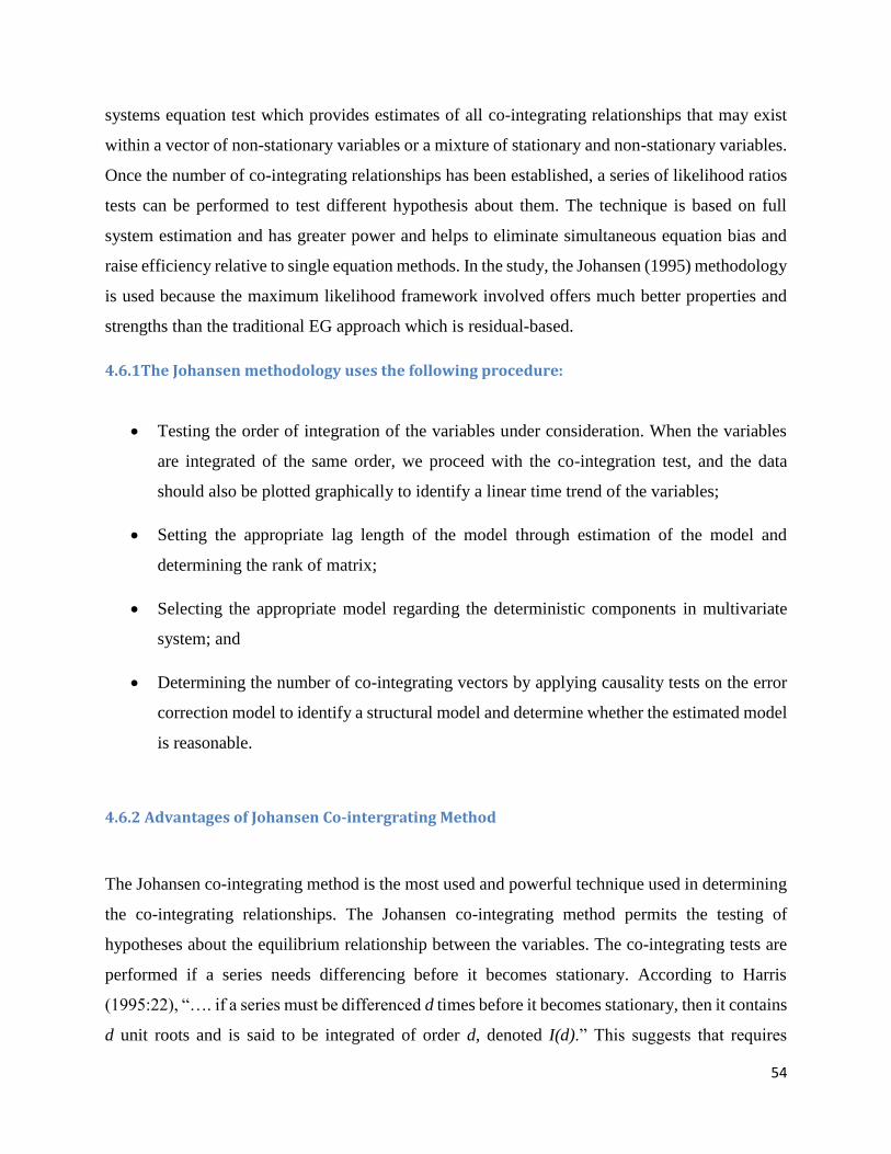
54
systems equation test which provides estimates of all co-integrating relationships that may exist
within a vector of non-stationary variables or a mixture of stationary and non-stationary variables.
Once the number of co-integrating relationships has been established, a series of likelihood ratios
tests can be performed to test different hypothesis about them. The technique is based on full
system estimation and has greater power and helps to eliminate simultaneous equation bias and
raise efficiency relative to single equation methods. In the study, the Johansen (1995) methodology
is used because the maximum likelihood framework involved offers much better properties and
strengths than the traditional EG approach which is residual-based.
4.6.1The Johansen methodology uses the following procedure:
Testing the order of integration of the variables under consideration. When the variables
are integrated of the same order, we proceed with the co-integration test, and the data
should also be plotted graphically to identify a linear time trend of the variables;
Setting the appropriate lag length of the model through estimation of the model and
determining the rank of matrix;
Selecting the appropriate model regarding the deterministic components in multivariate
system; and
Determining the number of co-integrating vectors by applying causality tests on the error
correction model to identify a structural model and determine whether the estimated model
is reasonable.
4.6.2 Advantages of Johansen Co-intergrating Method
The Johansen co-integrating method is the most used and powerful technique used in determining
the co-integrating relationships. The Johansen co-integrating method permits the testing of
hypotheses about the equilibrium relationship between the variables. The co-integrating tests are
performed if a series needs differencing before it becomes stationary. According to Harris
(1995:22), “…. if a series must be differenced d times before it becomes stationary, then it contains
d unit roots and is said to be integrated of order d, denoted I(d).” This suggests that requires

55
differencing before it becomes stationary is integrated of the order equivalent to the number of
times that series is differenced. The Johansen co-integration test, which is a Vector auto-regressive
(VAR) framework, provides a unified approach for the multivariate co-integration system based
on the error correction mechanism of the VAR (k) model.
4.7 Vector Error Correction Model (VECM)
In the event that co-integration is established in the study, the VECM is estimated to analyse the
short-term interaction between the variables of interest.
The VECM specifies the short-run dynamics of each variable in the system and in a framework
that anchors the dynamics to long-run equilibrium relationship suggested by economic theory. For
instance, the economic theory suggests that economic activity across regions should converge. If
this convergence hypothesis is true, we might observe long run relationships between employment
performances across regions. The existence of such long run conditions does not prevent the
existence of stationary, though variable short run deviation from them. Phillips and Perron (1998)
showed that forecasts based on a VEC model that explicitly estimates co-integrating relationships
and unit roots are consistent and asymptotically optimal.
4.8 Impulse Response
Impulse responses traces out the response of current and future values of each variable to a one
unit increase in the current value of one of the errors, assuming that this error returns to zero in
subsequent periods and that all other errors are equal to zero (Stock & Watson, 2006). Therefore,
for each variable from each equation separately, a unit shock is applied to the error, and the effects
upon the VAR system, over time, are noted. Thus, if there are g variables in a system, a total of
impulse responses could be generated. This is achieved, in practice, by expressing the VAR model
as a vector moving average (VMA). If the system is stable, the shock will gradually die away
(Brooks, 2008:299).
To determine the reaction of stock prices to changes in monetary policy, impulse response
functions were constructed from the VAR. Brooks (2008) points out that impulse response
functions trace out the responsiveness of the dependent variables in the VAR to shocks to each of

56
the variables. For each variable from each equation, separately, a unit shock is applied to the error,
and the effects upon the VAR system over time are noted. Thus, this helped us to analyze the
response of stock prices to changes in monetary policy for a unit shock in the other variables.
4.9 Variance Decomposition
In addition to the impulse response function results, we also conducted variance decomposition
analysis. Yinusa and Akinlo (2008) showed that while impulse response functions trace the effects
of a shock to one endogenous variable on to other variables in the VAR, variance decomposition
separates the variation in an endogenous variable into the component shocks to the VAR. The
variance decomposition analysis, thus, provides information about the relative importance of each
random innovation in affecting the variables in the VAR. Thus, in this study, variance
decomposition gave us the proportion of the movement in the stock prices versus shocks to other
variables. This helped us to identify factors which affect stock prices in the short, medium and
long run.
4.10 Diagnostic checks
Diagnostic checks are vital in the examination of the relationship between transport infrastructure
investment and unemployment variables because they validate the parameter evaluation outcomes
achieved by the estimated model. These checks test the stochastic properties of the model such as
residual auto-correlation, heteroscedasticity and normality, among others. The multivariate
extensions of the residual tests just mentioned are applied in this study and briefly discussed.
4.10.1 Normality Test
This is a test of normality that has now become very popular and is included in several statistical
packages is the Jarque-Bera (JB) test. This test first computes the coefficients of skewness and
kurtosis of a random variable. For a normally distributed variable, skewness is zero and kurtosis
is three (Gujarati, 2009).
The assumptions of the Classical Linear Regression Model (CLRM) require that the residuals are
normally distributed with zero mean, and a constant variance and violation of this restriction will

57
result in t-and F-statistics being not valid. One way of detecting mis-specification problems is
through observing the regression residuals. Usually, the normality test checks for skewness (third
moment) and excess kurtosis (fourth moment) (for details on the test, see Verbeek, 2000:173). The
Jarque-Bera normality test compares the third and fourth moments of the residuals to those from
the normal distribution under the null hypothesis that residuals are normally distributed, and a
significant Jarque-Bera statistic, therefore, points to non-normality in the residuals may not render
co-integration tests invalid.
4.10.2 Heteroscedasticity Test
This test is an extension of White’s (1980) test to systems of equations. It tests the null hypothesis
that the errors are both homoscedastic (no heterocedasticity problem) and independent of the
regressors and that there is no problem of mis-specification. The test regression is ran by regressing
each cross product of the residuals on the cross products of the regressors and testing the joint
significance of the regression. The failure of any one or more of the conditions just mentioned
above could lead to a significant test statistic. Thus, under the null of no Heteroscedasticity and no
misspecification, the test statistic should not be significant.
Heteroskedasticity arises if different error terms do not have identical variances, so that the
diagonal elements of the covariance matrix are not identical. The error terms are mutually
uncorrelated while the variance of μi may vary over the observations. The consequences of using
the usual testing procedures despite the heteroskedasticity are that the conclusions we draw or the
inferences we make may be very misleading (Gujarati, 2003:399). In this study, we employed the
White test. The general white test of heteroskedasticity does not rely on the normality assumption
and is easy to implement (Gujarati, 2003:413). The basis of this test is to check whether there is
any systematic relation between the squared residuals and the explanatory variables (Mukherjee
at al.1998:261). It tests the null hypothesis that there is no heteroskedasticity in which the test
statistic should not be significant in the absence of heteroskedacity and mis-specification.

58
4.10.3 Auto-relation Test
The term auto-correlation can be defined as correlation between members of observations ordered
in time series data. Auto-correlation is usually associated with time series data although as the
preceding definition suggests autocorrelation can occur in cross-sectional data. There is serial
correlation (i.e. auto-correlation) when either the dependent variable or the residual show
correlation with its values in pasts periods. This is a problem because standard errors are not
consistent, thereby affecting statistical inferences (i.e. Hypothesis testing). It arises in cases where
the data have a time dimension and where two or more consecutive error terms are related. In this
case, the error term is subject to auto-correlation or serial correlation. It arises as a result of either
excluded variables or the use of incorrect functional form. The consequences of auto-correlation
are that the OLS remains unbiased, but becomes inefficient and its standardized errors are
estimated in the wrong way (Gujarati, 2003: 454; Verbeek, 2000:90).
The study applied the Lagrange Multiplier (LM) test, a multivariate test statistic for residual serial
correlation up to the specified lag order. Harris (1995: 82) argues that the lag order for this test
should be the same as that of the corresponding VAR. The Lagrange Multiplier (LM) tests the null
hypothesis, H0: ρ1=ρ2= ……. =ρp=0 (no auto-correlation) against the alternative hypothesis, H1:
at least one of the ρs is not zero, thus serial correlation.
4.11 CONCLUDING REMARKS The chapter presented the procedures involved in the Johansen (1988), Johansen and Juselius
(1990) approach. The co-integration technique has been chosen as the preferred parameter
estimation technique for monetary policy model. This is because of its several advantages over
alternative techniques. Based on the co-integration approach, the error correction model, which
contains information on both the long run and short run relationship between variables is estimated.
The estimated model has to pass all the diagnostic checks which involve the auto-correlation LM
test, white heteroskedasticity test and residual normality test. Having familiarized ourselves with
the estimation techniques, we now apply these techniques to South African data in order to achieve
the objectives of this study as set out in Chapter one.

59
CHAPTER FIVE
ESTIMATION AND INTERPRETATION OF RESULTS
5.1 Introduction
The main aim of this chapter is to present, interpret and analyze all the tests results. This chapter
also applies the techniques discussed previously using South African data in order to achieve the
objectives set out in Chapter 1. It amplifies the trends analysis of Chapter 2 by applying the
analytical techniques proposed on annual data covering 1982 to 2012. The results presented
include those of unit root and co-integration. Assuming the presence of at least one co-integration
relationship among the variables, the error correction model (VECM) is estimated; otherwise VAR
analysis is done. After the VECM and VAR analysis, the study moves on to carry out diagnostic
checks to ensure the adequacy of the model. The econometric package used in this study is the E-
views version.
5.2 Informal Unit Root Tests
5.2.1 Graphical displays
A popular informal test for Stationarity is the graphical analysis of the series. This is a visual plot
of the series which is an important step in the analysis of time series before pursuing any formal
tests. This introductory examination of the data is important as it allows the recognition of any
data capturing errors and structural breaks and gives an idea of the trends and Stationarity of the
data set. Figure 5.1 below displays plots of all variables considered for the unemployment model.
Figure 5.1 below shows five of the series (Unemployment, RGDP, RExch, OPEN,Ri) are trending
upwards with some fluctuations while the rest of the series (transport infrastructure investment and
total infrastructure – transport infrastructure investment) do not show any trend, notwithstanding
huge fluctuations.
All other variables in figure 5.1 follow a stationary process-white noise process as it moves closely
around the mean and could be stationary or closer to the stationary boundary; it also seems to be

60
hovering around its mean, but the variance is clearly not constant over time. Except for the
variables Unemployment, GDP and OPEN, they have a time variant mean and variance suggesting
that they are not stationary in their levels.
Figure 5. 1: Graphical unit root tests 1982-2012
5.2.1i Stationarity test: levels
10
15
20
25
30
35
1985 1990 1995 2000 2005 2010
UNEMPL
-20
-10
0
10
20
30
40
1985 1990 1995 2000 2005 2010
Tran INFR INVE
8
10
12
14
16
18
20
22
1985 1990 1995 2000 2005 2010
RGDP
-30
-20
-10
0
10
20
30
1985 1990 1995 2000 2005 2010
REXCH
40
60
80
100
120
1985 1990 1995 2000 2005 2010
OPEN
-30
-20
-10
0
10
20
30
1985 1990 1995 2000 2005 2010
Tti-Ti
-4
0
4
8
12
16
1985 1990 1995 2000 2005 2010
RI
Based on this analysis above, we cannot be certain of the stationarity of the variables, especially
those that do not follow a clear trend such as transport infrastructure investment in this study.
Therefore, more analysis is required.

61
Figure 5.2: Graphical unit root tests 1982-2012
5.2.1.ii Stationarity test: differenced
-8
-6
-4
-2
0
2
4
6
1985 1990 1995 2000 2005 2010
Differenced UNEMPL
-30
-20
-10
0
10
20
30
40
1985 1990 1995 2000 2005 2010
Differenced Tran INFR INVE
-5
-4
-3
-2
-1
0
1
2
1985 1990 1995 2000 2005 2010
Differenced RGDP
-30
-20
-10
0
10
20
30
40
1985 1990 1995 2000 2005 2010
Differenced REXCH
-30
-20
-10
0
10
1985 1990 1995 2000 2005 2010
Differenced OPEN
-40
-20
0
20
40
60
1985 1990 1995 2000 2005 2010
Differenced Tti-Ti
-8
-4
0
4
8
12
1985 1990 1995 2000 2005 2010
Differenced RI
Figure 5.2 shows the time series data at first differencing. The trends from the variables
(Unemployment, Tii, RGDP, RExch, OPEN, Ri and TT-Tii) follows a stationary process-white
noise process, as they move closely around the mean. Formal tests stationarity are used to augment
informal graphical analysis of stationarity. These formal tests are discussed in the subsequent
section.
5.2.2 Testing for Stationarity/ Unit Root

62
The formal tests used in this study are the Augmented Dickey (ADF) and Phillips-Peron (PP). The
results of these tests are reported in table 5.1, and these confirmed that differencing once was all
that was required to bring these variables to stationarity.
These tests were applied to the data under different deterministic trend assumptions, that is, those
that excluded constant and trend and have trend and intercept produced robust results. The option
with constant and no trend produced ‘explosive’ results (especially under the ADF).
Granger and Newbold (1974) argued that when the dependent and independent variables have unit
roots, traditional estimation methods using observations on levels of those variables will likely
find a statistically significant relationship, even when a meaningful economic linkage is absent.
For meaningful policy analysis, it is important, therefore, to distinguish between a correlation that
arises from a shared trend and one associated with an underlying causal relationship. Thus, in this
study, to achieve that, the data was subjected to two types of tests to establish their univariate time
series behaviour in order to determine the basic unit of observation. These tests are the Augmented
Dickey-Fuller (ADF) and Phillips-Perron (PP).
The unit root tests considered both the null hypothesis of a random walk without a drift
(untrended) and a random walk with a drift (trended). The results of these tests are reported in
Table 5.1.
In this section, we follow the estimation techniques developed in the analytical framework given
in Chapter 4. Thus, the following step involves subjecting the variable to stationarity.
The results are shown in table 5.1 below:
Table 5.1: Unit root tests 1982-2012 at levels and first differences (Δ)
Variables Augmented Dickey-Fuller (ADF) Phillips Peron (PP) Ord
er of
Inte
grati
on
INTERCEP
T
TREND
AND
NONE INTERCEP
T
TREND
AND
NONE

63
INTERCEP
T
INTERCEP
T
UNEMPL
Δ(UNEMP
L)
-5.242942***
-6.528687***
-5.354462***
-6.398641***
0.731969*
-5.131256***
-2.342435*
-5.441617***
-2.056712
-
7.554440***
0.853910
-
5.135623*
**
I(1)
Ti
Δ (Ti)
-4.691293***
-8.265613***
-4.987490***
-8.142329***
-3.523379***
-8.414018***
-4.683783***
-18.54074***
-
4.946772***
-
19.48874***
-
3.466719*
**
-
17.66655*
**
I(0)
RGDP
Δ (RGDP)
-4.771845***
-4.479275***
-0.488928
-5.213531***
0.832469
-4.627427***
-1.680152
-4.759339***
-0.511978
-
5.300405***
0.773073
-
4.619777*
**
I(1)
RExch
Δ(RExch)
-4.982391***
-6.937591***
-4.921890**
-6.763648***
-5.052861***
-7.069887***
-6.109283***
-18.34451***
-
7.267285***
-
18.12989***
-
6.103292*
**
-
17.19374*
**
I(0)
Ri
Δ (Ri)
-2.794733*
-6.739867***
-2.922135
-6.677872***
-1.047434
-6.893383***
-2.857881*
-6.878240***
-2.993088
-
6.664359***
-0.795720
-
7.042366*
**
I(0)
OPEN
Δ(OPEN)
-5.623352***
-5.390222***
-5.511715***
-5.457232***
1.937265*
-5.530860***
-0.228826
-7.517259***
-2.915481
-
7.273865***
3.025153*
**
-
4.838943*
**
I(1)
Tti-Ti
Δ(Tti-Ti)
-4.690509***
-6.257001***
-5.813699***
-6.123816***
-4.746631***
-6.300522***
-4.685112***
-22.14774***
-
6.248874***
-
21.50399***
-
4.742778*
**
-
17.91749*
**
I(0)

64
Critical
Values 1%
5%
10%
-3.670170
-2.963972
-2.621007
-4.309824
-3.574244
-3.221728
-2.647120
-1.952910
-1.610011
-3.670170
-2.963972
-2.621007
-4.296729
-3.568379
-3.218382
-2.644302
-1.952473
-1.610211
Values marked with *** represent a stationary variable at a 1% significance level, and **
represents a stationary variable at a 5% significant level. * 10% significant level.
The results in Table 5.1 show that the null hypothesis of non-stationarity cannot be rejected when
variables are at levels. When the test is applied to first differences of the series, they all become
stationary. We, therefore, can conclude that the variables in our co-integration regression are first
difference stationary, that is, each series is characterized as integrated of order one I(I).
The graphical analysis serves as a benchmark for the formal measure of the unit root. Table 5.1
shows that it is apparent that the series (transport infrastructure investment, real exchange rate, real
interest rate, and total infrastructure investment - transport infrastructure investment) are stationary
at levels, except for variables of unemployment, real gross domestic product, and openness which
exhibit non-stationarity at level series.
The indication of stationarity of variables means that variables exhibit some fluctuations around a
zero mean.
5.3 VAR Lag Length Selection Criteria
Dimitrious and Hall (2001) state that the issue of finding the appropriate lag length is of importance
because a model has to have standard normal error terms that do not suffer from non-normality,
auto-correlation, and heteroskedasticity.
The most common procedure in choosing the optimal lag is to estimate a VAR model including
all the variables in levels (non-differenced data). This VAR model should be estimated for a large
number of lags, then reducing down by re-estimating the model for one lag less until zero lags are
reached.

65
The common information criteria are the: Akaike Information Criteria (AIC), Schwarz Information
Criterion (SIC), Hannan-Quinn Information Criterion (HQI), Final Prediction Error (FPE) and the
Likelihood Ratio test (LR). An optimal lag length suggested by the above information criteria can
be chosen as these criteria may sometimes produce conflicting lag length choices. However,
decisions about the lag structure of a VAR model could be based on the fact that a given criterion
produces a white noise residual and conserves degrees of freedom. Table 5.2 below presents the
selection of an optimal lag length for this study.
Table 5.2: VAR Lag Order Selection Criteria
VAR Lag Order Selection Criteria
Endogenous variables: UNEMPL Tii RGDP REXCH OPEN RI TT_Tii
Exogenous variables: C
Date: 08/28/14 Time: 15:46
Sample: 1982-2012
Included observations: 116
Lag LogL LR FPE AIC SC HQ
0 -2507.646 NA 1.59e+10 43.35597 43.52213 43.42342
1 -1313.421 2223.730 42.39801 23.61071 24.94003 24.15033
2 -1165.265 257.9953 7.738270 21.90112 24.39360
*
22.91293
3 -1136.048 47.35226 11.12957 22.24220 25.89783 23.72618
4 -1113.612 33.65399 18.37232 22.70021 27.51899 24.65636
5 -904.1923 288.8547 1.242791 19.93435 25.91629 22.36267
6 -794.3783 138.2141
*
0.486826
*
18.88583
*
26.03092 21.78633
*
7 -761.8590 37.00467 0.760859 19.16998 27.47823 22.54266

66
8 -725.0231 37.47107 1.180027 19.37971 28.85111 23.22456
* indicates lag order selected by the criterion
LR: sequential modified LR test statistic (each test at 5%
level)
FPE: Final prediction error
AIC: Akaike information
criterion
SC: Schwarz information
criterion
HQ: Hannan-Quinn information criterion
In the empirical analysis, the choice of optimal lag length to be used in the estimation is imperative,
especially in a VAR model. This is important to avoid spurious rejection or acceptance of estimated
results. In addition, the lag length also influences the power of rejecting the null hypothesis. As
reported in table 5.2, the information criterion are the Akaike Information Criteria (AIC), Schwarz
Information Criterion (SIC), Hannan-Quinn Information Criterion (HQI), Final prediction error
(FPE) and the Likelihood Ratio test (LR). Of the available information criteria, the LR test is
regarded as the best approach in determining the lag length. Unlike the other information criteria,
the LR is a formal test whilst the other information criteria operate like the adjusted R2 measuring
the goodness of fit of the model. However, the LR performs the best, given a bigger sample size.
Thus, it is more reliable, given a bigger sample.
However, in the event that the information criteria produces conflicting results, Asteriou and Hall
(2011) argue that decisions about the lag structure of a VAR model could be based on the fact that
a given criterion produces a white noise residual and conserves degrees of freedom. In addition,
Takaendesa (2006) argues that if there is no consensus from the information criteria, there is no
conclusion which can be reached based on the multivariate approach. The standard approach
would be to examine the model with the different lags.

67
The lag length results in Table 5.2 shows that a lag 2 is chosen by one information criterion,
namely, the Schwarz information criterion (SC); lag 6 is chosen by four information criteria,
namely, the sequential modified (LR) test statistic (each test at 5% level), Final prediction error
(FPE), Akaike information criterion (AIC) and Hannan-Quinn information criterion (HQ). We
therefore, chose a lag of 6.
5.4 Johansen Co-integration Test and the Vector Error Correction Model
Results
5.4.1 Johansen Co-integration
Having tested for Stationarity and lag length and found that all variables I (1) were stationary
(except for Unemployment, GDP and OPEN) at 0.05 and 0.01 levels of significance, we tested for
possible co-integration among these variables.
The study applied the multivariate co-integration technique developed by Johansen and Juselius
(1990) to the system variables. The Johansen was chosen based on the fact that it performs better
than single-equation and alternative multivariate methods (lbrahim, 2000). The results of the Co-
integration tests are reported in Table 5.5 below.
Table 5.3: Johansen Co-integration Test results
Date: 09/01/14 Time: 11:27
Sample (adjusted): 1983-2012
Included observations: 119 after adjustments
Trend assumption: Linear deterministic trend
Series: UNEMPL Tii RGDP REXCH OPEN RI TT_Tii
Lags interval (in first differences): 1 to 4
Unrestricted Co-integration Rank Test (Trace)
Hypothesiz
ed
Trace 0.05
No. of
CE(s)
Eigenvalue Statistic Critical
Value
Prob.**
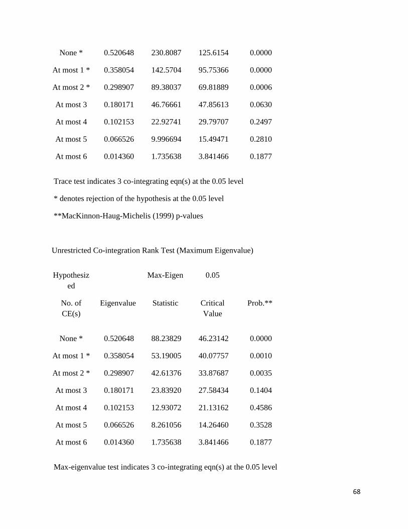
68
None * 0.520648 230.8087 125.6154 0.0000
At most 1 * 0.358054 142.5704 95.75366 0.0000
At most 2 * 0.298907 89.38037 69.81889 0.0006
At most 3 0.180171 46.76661 47.85613 0.0630
At most 4 0.102153 22.92741 29.79707 0.2497
At most 5 0.066526 9.996694 15.49471 0.2810
At most 6 0.014360 1.735638 3.841466 0.1877
Trace test indicates 3 co-integrating eqn(s) at the 0.05 level
* denotes rejection of the hypothesis at the 0.05 level
**MacKinnon-Haug-Michelis (1999) p-values
Unrestricted Co-integration Rank Test (Maximum Eigenvalue)
Hypothesiz
ed
Max-Eigen 0.05
No. of
CE(s)
Eigenvalue Statistic Critical
Value
Prob.**
None * 0.520648 88.23829 46.23142 0.0000
At most 1 * 0.358054 53.19005 40.07757 0.0010
At most 2 * 0.298907 42.61376 33.87687 0.0035
At most 3 0.180171 23.83920 27.58434 0.1404
At most 4 0.102153 12.93072 21.13162 0.4586
At most 5 0.066526 8.261056 14.26460 0.3528
At most 6 0.014360 1.735638 3.841466 0.1877
Max-eigenvalue test indicates 3 co-integrating eqn(s) at the 0.05 level

69
* denotes rejection of the hypothesis at the 0.05 level
**MacKinnon-Haug-Michelis (1999) p-values
Notes
Both the Trace test and Ma-Eigen Statistic indicate 3 Co-integrating equations at a 0.05
level of significance;
*denotes rejection of the null hypothesis at 0.05 level of significance;
The series of estimation are: UNEMPL, Tii, RGDP, REXCH, OPEN, RI, TT_Tii, and
critical values are from Mcknnon-Haug-Michells (1999); and
The results are based on the assumption of a constant linear trend in the data with optimal
lag length 4.
Source: Author’s Computation using Eviews 7 Econometric Package
From table 5.3 above, the null hypothesis of no co-integration was rejected at a 0.05 level of
significance. This indicates that there are four co-integrating relationships among variables:
Unemployment, Transport infrastructure investment, Real gross domestic product, Real
exchange rate, Real interest rate, Openness, and Total infrastructure investment minus
transport infrastructure investment. This implies an existence of a long run relationship among
the variables in the study. Therefore, a Vector Error Correction Model (VECM) can be
specified from the results of the regression analysis.
The study proceeded to estimate a VECM normalized on Unemployment where unemployment
is a dependent variable.
5.5 The long run regression results
Table 5.5.1: The long run regression result table
Variable Coefficient Standard
error
T-Stat

70
Constant -28.33393 - -
Unemployment 1.000000 - -
Tii 2.761845 0.51312
5.38243
RGDP 2.716086 1.06291 -2.55533
RExch 0.153478 0.22730 0.67522
Ri -2.095376 0.66100
3.17003
OPEN 0.294578 0.19537 1.50778
TT-Tii 4.009540 0.56342 -7.11641
Source: Author’s own computation using Eviews 7
The results from the table above show the long-run relationship between explanatory variables
(Tii, RGDP, RExch, Ri, OPEN and TT-Tii) and the dependent variable Unemployment. From the
findings, the long-run co-integrating equation can be estimated as follows:
Unemplt = - 28.33393 - 2.761845Tii - 2.716086RGDP - 0.153478RExch + 2.095376Ri
-0.294578OPEN - 4.009540TT-Tii + µt………………………...……………………...…….. (5.1)
The standard procedure in interpreting the long-run VECM results was applied. All the variables
enter the long-run equation significantly, and the signs and magnitudes also appear reasonable. In
particular, the results suggest that transport infrastructure investment and other variables have a
negative impact on unemployment in South Africa. However, real interest rates have a positive
effect on unemployment in South Africa.
As indicated on the long-run equation, transport infrastructure investment is significant in
specification; the negative coefficient of the variable in the regression suggests that an increase in
investment in the transport infrastructure will lead to a decrease in unemployment, as suggested
by the labour market theories. Smith (2003) states that if government spends more on the transport
infrastructure, this would decrease unemployment.
RGDP, as a measure of economic activity, is significant in the specification model, and the
negative coefficient in the regression suggests that a decrease in RGDP will result in an increase

71
in unemployment. This is consistent with the a priori expectation that during the economic
downswing, unemployment shows upward sloping or becomes positively sloped. When there is a
decline in real gross domestic product, the unemployment rate becomes possibly (Barker, 2007).
Real exchange rate, as a measure of external balances, is significant. The negative coefficient in
the regression suggests that a decrease in real exchange rate will lead to an increase in
unemployment. If the rand depreciates, exports are expected to increase, thereby increasing
economic growth, which will lead to job creation. If the rand appreciates, exports are expected to
decrease, thereby decrease economic growth which will lead to less jobs; imports are expected to
increase causing a deterioration of the current account in the balance of payment, and this may
result in a decline in economic growth (Appleyard & Field, 2005). This does corroborate the a
priori expectations.
Real interest rates have a positive relationship in the regression results, thus indicating that an
increase in real interest rates will lead to an increase in unemployment. This does corroborate the
a priori expectations, as supported by Phillips’ curve theory which states that there is a positive
relationship between real interest rate and unemployment; as real interest rate increases
unemployment will also increase (Phillips, 1958).
Trade openness was expected to be negative or positive in the a priori expectations. There is a
negative relationship in the regression results indicating that a decrease in trade openness will lead
to an increase in unemployment of the country.
TT-Tii is significant in the specification model, and the negative coefficient in the regression
suggests that a decrease in TT-Tii will result in an increase in the unemployment; this corroborates
the a priori expectations.

72
Figure 5.4: Co-integration Graph
-60
-40
-20
0
20
40
60
82 84 86 88 90 92 94 96 98 00 02 04 06 08 10 12
Cointegrating relation 1
Source: Author’s own computation using Eviews 7
The residual tests of the co-integrating equation are stationary, graphically. From the graph above,
the residuals are stationary further confirming the goodness of fit of our model.
5.5.2 Short run relationships: Error- Correction Model
Short run analysis is intended to capture the short run determinants of unemployment. Comparing
the coefficients of the error correction terms (CointEq1), of Table 5.5 below, for the first Vector
shows that the D(TT-Tii) has the most significant coefficient and has a correct positive sign. Other
variables have less significance, suggesting that the total investment minus transport investment
equation constitutes the true co-integrating relationship in the first co-integration vector in Table
5.
Table 5.5: Vector Error Correction
Error Correction: D(UNEMPL) D(Tii) D(RGDP) D(REXCH) D(OPEN) D(RI) D(TT_Tii)
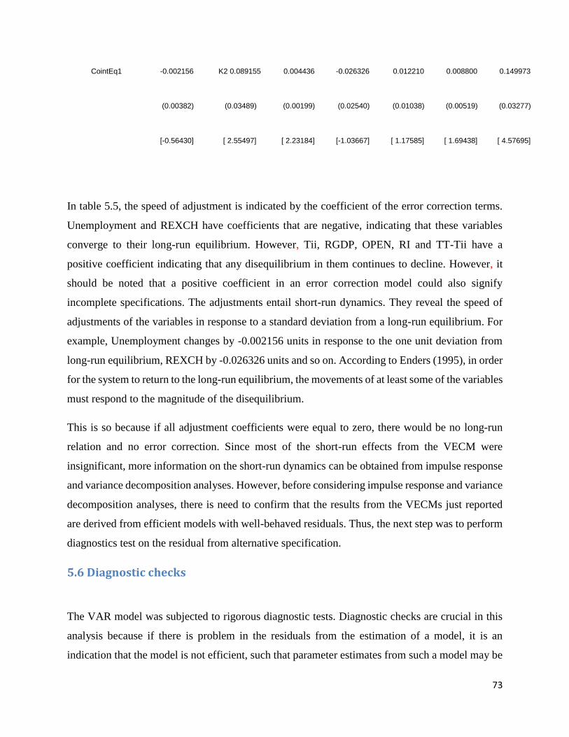
73
CointEq1 -0.002156 K2 0.089155 0.004436 -0.026326 0.012210 0.008800 0.149973
(0.00382) (0.03489) (0.00199) (0.02540) (0.01038) (0.00519) (0.03277)
[-0.56430] [ 2.55497] [ 2.23184] [-1.03667] [ 1.17585] [ 1.69438] [ 4.57695]
In table 5.5, the speed of adjustment is indicated by the coefficient of the error correction terms.
Unemployment and REXCH have coefficients that are negative, indicating that these variables
converge to their long-run equilibrium. However, Tii, RGDP, OPEN, RI and TT-Tii have a
positive coefficient indicating that any disequilibrium in them continues to decline. However, it
should be noted that a positive coefficient in an error correction model could also signify
incomplete specifications. The adjustments entail short-run dynamics. They reveal the speed of
adjustments of the variables in response to a standard deviation from a long-run equilibrium. For
example, Unemployment changes by -0.002156 units in response to the one unit deviation from
long-run equilibrium, REXCH by -0.026326 units and so on. According to Enders (1995), in order
for the system to return to the long-run equilibrium, the movements of at least some of the variables
must respond to the magnitude of the disequilibrium.
This is so because if all adjustment coefficients were equal to zero, there would be no long-run
relation and no error correction. Since most of the short-run effects from the VECM were
insignificant, more information on the short-run dynamics can be obtained from impulse response
and variance decomposition analyses. However, before considering impulse response and variance
decomposition analyses, there is need to confirm that the results from the VECMs just reported
are derived from efficient models with well-behaved residuals. Thus, the next step was to perform
diagnostics test on the residual from alternative specification.
5.6 Diagnostic checks
The VAR model was subjected to rigorous diagnostic tests. Diagnostic checks are crucial in this
analysis because if there is problem in the residuals from the estimation of a model, it is an
indication that the model is not efficient, such that parameter estimates from such a model may be

74
biased. The VAR was tested for AR Roots test and serial correlation, and the results are indicated
in Figure 5.4 below.
Figure 5.4 AR Roots Graph
The AR Roots Graph reports the inverse roots of the characteristic AR polynomial. The estimated
VAR is stable (stationary) if all roots have modulus less than one and lie inside the unit circle. If
the VAR is not stable, certain results such as impulse response standard errors are not valid. Figure
5.4 shows that all roots lie inside the unit circle, which is an indication that our VAR is stable.
Of importance in this analysis are the residual diagnostic checks for serial correlation, normality
and heteroskedasticity. As mentioned in Chapter 4, the three tests are based on the null hypothesis
that there is no serial correlation, there is no normality and there is no heteroskedasticity problem
for the LM, Jarque-Bera and White heteroskedasticity tests, respectively.
5.6.1 Auto-correlation LM test
-1.5
-1.0
-0.5
0.0
0.5
1.0
1.5
-1.5 -1.0 -0.5 0.0 0.5 1.0 1.5
Inverse Roots of AR Characteristic Polynomial

75
The Lagrange Multiplier (LM) test was carried out to check for auto-correlation based on residual
auto covariances. The null hypothesis of the test is that there is no serial correlation in the residuals
up to the specified lag order.
Table 5.6: Langrange Multiplier Test results
VEC Residual Serial Correlation LM Tests
Null Hypothesis: no serial correlation at lag
order h
Date: 08/28/14 Time: 16:35
Sample: 1982-2012
Included observations: 30
Lags LM-Stat Prob
1 42.09273 0.7471
2 62.37848 0.0949
3 39.85503 0.8212
4 195.1493 0.0000
5 45.84075 0.6020
6 39.00083 0.8461
7 18.23311 1.0000
8 309.6684 0.0000
9 55.43142 0.2451
10 31.25139 0.9773
11 24.46229 0.9987
12 224.8972 0.0000
Probs from chi-square with 49 df.
There is serial correlation when the residuals show correlation with its values in past periods. A
zero probability value would indicate the presence of serial correlation and if the probability of the

76
LM statistic is high, we fail to reject the null that there is no serial correlation. In the above table,
probability of 0.8461 is high (greater than 0.05). Therefore, we fail to reject the null hypothesis
and, thus, conclude: there is no serial correlation among our variables.
Table 5.7: Residual Normality Test
Null hypothesis: Residual are multivariate normal
Chi-Squ P-Value
Skewness 1.722483 0.1894
Kurtosis 2.279648 0.1311
Jarque Bera 4.002132 0.1352
The probabilities of the Kurtosis (p-value 0.1311) and Skewness (p-value 0.1894) are both
insignificant, thus we fail reject the null hypothesis which is a clear indication of normality. The
diagnostic test results reveal that the model is relatively well-specified. The study moved on and
checked the impulse response and variance decomposition of the series.
5.7 Other Diagnostic Tests
Table 5.8 Diagnostic Tests
Test H0 Conclusion
Jarque-Bera Residuals are
normally
distributed
Errors are
normally
distributed
VEC Residual Serial
Correlation LM Tests
There is no serial
Correlation in the residuals.
No 2nd-order auto-
correlation
VEC Residual Heteroskedasticity
Tests
The residuals are
homoscedastic
No
Heteroskedasticity

77
Table 5.8 shows that the results do not suffer from auto-correlation, non-normality and
heteroscedasticity. The results obtained from analysis are, therefore, robust.
5.8 Impulse response of Unemployment to its independents
Since this study focuses on the determinants of the yield curve, only the responses of the yield
spread to shocks in its determinants are reported in figure 5.5. These impulse response functions
show the dynamic response of the real exchange rate to a one-period standard deviation shock to
the innovations of the system and also indicate the directions and persistence of the response to
each of the shocks over a 32 year period.
Thus, as indicated in chapter 4, the impulse response function traces the temporal and directional
response of an endogenous variable to a change in one of the structural innovations. Impulse
response functions give an indication of the lag structure in the economy, showing the responses
of a particular variable to a one-time shock in each of the variables in the system. It follows that
the interpretation of the impulse response functions should take into consideration the use of first
differencing of the variables as well as the vector error correction estimates. Thus, a one-time
shock to the first difference in a variable is a permanent shock to the level of that variable.

78
Figure 5.5: Impulse response of Unemployment to its independents
To outline the responsiveness of the dependent variable (Unemployment) in a VAR to shocks from
each of the explanatory variables (Tii, RGDP, REXCH, OPEN, RI and TT_Tii), impulse response
tests are employed. In the study, impulse response analysis traces out the responsiveness of
Unemployment to unanticipated shocks from its explanatory variables. Figure 5.5 shows the
results of impulse response analysis in this study.
The response of unemployment to its own shocks show that from 1982, the response was positive
and increasing, and during 1990, it started decreasing but still remained positive. After 2002, it
then started showing a constant trend up until 2012.
5.9 Variance decomposition of unemployment to its explanatory variables
As mentioned in Chapter 4, variance decomposition analysis provides a means of determining the
relative importance of shocks in explaining variations in the variable of interest. In the context of
-1.0
-0.5
0.0
0.5
1.0
1.5
5 10 15 20 25 30
Response of UNEMPL to UNEMPL
-1.0
-0.5
0.0
0.5
1.0
1.5
5 10 15 20 25 30
Response of UNEMPL to TRAN_INFR_INVE
-1.0
-0.5
0.0
0.5
1.0
1.5
5 10 15 20 25 30
Response of UNEMPL to RGDP
-1.0
-0.5
0.0
0.5
1.0
1.5
5 10 15 20 25 30
Response of UNEMPL to REXCH
-1.0
-0.5
0.0
0.5
1.0
1.5
5 10 15 20 25 30
Response of UNEMPL to OPEN
-1.0
-0.5
0.0
0.5
1.0
1.5
5 10 15 20 25 30
Response of UNEMPL to RI
-1.0
-0.5
0.0
0.5
1.0
1.5
5 10 15 20 25 30
Response of UNEMPL to TTI_TI
Response to Cholesky One S.D. Innovations
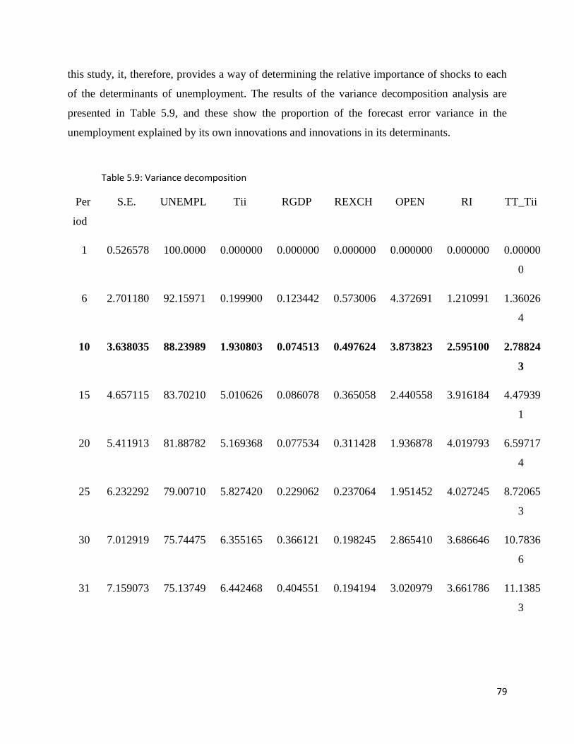
79
this study, it, therefore, provides a way of determining the relative importance of shocks to each
of the determinants of unemployment. The results of the variance decomposition analysis are
presented in Table 5.9, and these show the proportion of the forecast error variance in the
unemployment explained by its own innovations and innovations in its determinants.
Table 5.9: Variance decomposition
Per
iod
S.E. UNEMPL Tii RGDP REXCH OPEN RI TT_Tii
1 0.526578 100.0000 0.000000 0.000000 0.000000 0.000000 0.000000 0.00000
0
6 2.701180 92.15971 0.199900 0.123442 0.573006 4.372691 1.210991 1.36026
4
10 3.638035 88.23989 1.930803 0.074513 0.497624 3.873823 2.595100 2.78824
3
15 4.657115 83.70210 5.010626 0.086078 0.365058 2.440558 3.916184 4.47939
1
20 5.411913 81.88782 5.169368 0.077534 0.311428 1.936878 4.019793 6.59717
4
25 6.232292 79.00710 5.827420 0.229062 0.237064 1.951452 4.027245 8.72065
3
30 7.012919 75.74475 6.355165 0.366121 0.198245 2.865410 3.686646 10.7836
6
31 7.159073 75.13749 6.442468 0.404551 0.194194 3.020979 3.661786 11.1385
3

80
32 7.301982 74.55254 6.536267 0.444218 0.191002 3.161807 3.651374 11.4627
9
Cholesky Ordering: UNEMPL Tii RGDP REXCH OPEN RI TT_Tii
The variance decomposition is reported over 32 quarters. The results show that for the 32 periods,
the predominant source of variation in unemployment is own shock, which accounts for between
80% and 100%. This is consistent with Brooks (2002) and Goyenko et al (2008). Another
important source of variation in unemployment is total infrastructure investment-transport
investment, which accounts for nearly 12% in the variation in the long-run. Transport
infrastructure investment and real interest rate are also important factors determining
unemployment; this is consistent with a priori expectations and supports the long-run results.
5.10 Conclusion
This chapter focused on interpreting the results of models estimated in chapter 4. The chapter
began with analyzing the time series properties of the data using three methods of testing for unit
root. All two methods confirmed that the variables are integrated of order one I(1). Having
determined the order of integration of the variables, the lag length used in the estimation for the
Johansen co-integration was determined empirically, with the majority of the information criteria
settling for the lag of 1 whilst the LR suggested a lag of 6. The two lag lengths were, therefore,
used in the estimation. At a lag of two, the Johansen co-integration test established that there is
one co-integrating equation whilst at a lag of 6, there were seven (3) co-integrating equations. This,
therefore, implied that there is a long-term relationship between unemployment and its
determinants. The VECM was also estimated to analyze both the long-run and the short-run
interaction between the variables. The long-run equation showed that all the variables employed
in the model are significant and carried the correct signs. The results established that financial
sector development has facilitated the accumulation of unemployment in South Africa, which was
the aim of the study. These results were all confirmed by the variance decomposition. The results
also observed all the assumptions which underlie the classical linear regression model.

81
CHAPTER SIX
STUDY SUMMARY, CONCLUSIONS, POLICY IMPLICATIONS AND
RECOMMENDATIONS
6.1 Introduction
This chapter focuses on conclusion based on the results of the study and makes recommendations
for future policy formulation as well as articulates the implications of the findings on South Africa
and the global context on developing and emerging market economies.
6.2 Summary of the study and conclusions
The purpose of this study was to investigate the nature of the relationship between transport
infrastructure investment and unemployment in South Africa using the annual data from the period
of 1982-2012. The study also reviewed whether the trends of unemployment in transport
infrastructure investment, RGDP, REXCH, OPEN, RI, TT_Tii are closely related.
Chapter 3 reviewed theoretical and empirical literature which looked at demand for labour, supply
of labour, standard competitive model and structural unemployment. These theories complement
each other in that the limitation of one theory is overcome by the advantage of the other. Some
empirical studies supported the theoretical foundations that there is a positive relationship between
transport infrastructure investment and unemployment did receive sufficient attention in the South
African studies that were reviewed. Most of the empirical literature looked at transport
infrastructure investment and economic growth in South Africa; there are few studies which looked
at unemployment in South Africa.
The explanatory variables used in this study are: transport infrastructure investment, real gross
domestic product, real exchange rate, real interest rate, trade openness, and total infrastructure
investment minus transport infrastructure investment. All these explanatory variables carried

82
coefficient signs that conformed to unemployment. Annual data for the period 1982-2012 was used
for the purpose of running a regression.
In order to determine both long-run properties of the models, the Johansen co-integration and error
correction methods were preferred to the other techniques. These techniques were chosen because
of the advantages they have over those alternative techniques. In applying these methods, the time
series was subjected to both informal and formal tests for stationarity. The variables in the co-
integration regression were found to be first difference stationary, that is, each series is
characterized as integrated of order on I(1). Johansen co-integration tests provided evidence that
there is co-integration between unemployment and its targets, which were included in these
models. Evidence of co-integration allowed the estimation of VECM’s, which simultaneously
provided the parameter estimated for both the long-run and short-run. In both cases, the estimated
models were robust and passed all the relevant diagnostic test. The results conform to theoretical
literature reviewed for the study.
6.3 Policy recommendations and areas of further study
The results of the study revealed a number of policy implications which affect transport
infrastructure investment and unemployment. A negative relationship between transport
infrastructure investment and unemployment means that if transport infrastructure investment
increases, unemployment will decrease, and there is an inverse relationship between the two
variables.
This study, therefore, recommends that efforts should be made to lower the level of unemployment
in South Africa. To this end, the government of South Africa should invest more on the transport
infrastructure as it is an important engine to reduce unemployment. The policies that focus on
transport infrastructure will, in turn, increase the economic growth of South Africa, meaning that
the more resources the government spends on transport infrastructure, the more growth in the
economy.
It is recommended that the government should improve the transport infrastructure in both rural
and in urban areas as this will lead to a decline in the level of unemployment in South Africa.

83
6.4 Limitations of the study and areas for further research
The study focused on selected macro-economic variables determining the unemployment in South
Africa that can be accommodated by the models. Furthermore, this work only considered the
period of 1982 up to 2012. The study is limited to the South African economy, and the consequence
is that the results obtained may not be directly applicable to other economies. Nonetheless, the
study remains significant as the conclusions draw from it may prove to be useful in South Africa
context. Applications to other economies must be done with caution, given different economic
structures and the nature of the monetary policy and interest rate regimes.

84
REFERENCES
Akinlo, A.E. (2003). Assessing the impact of Nigeria’s naire depreciation on output and inflation.
Applied Economics, 1/1/2003.
Appleyard, D.R., Cobb S.L. & Field A.J. (2010). International economics (7th edition). New York:
McGraw Hill international.
Aschauer, D.A. (1989). Is public expenditure productive? Journal of Monetary Economics, 23(2):
177‐200.
Bangane, T. (1999). The Unemployment problem in South Africa with specific reference to the
Lekoa Vaal Triangle Metropolitan Area (LVTMA), Johannesburg.
Barker, F. (2003). The South African Labour Market (4th edition). Hatfield, South Africa
Barker, F. (2007). The South African Labour Market Theory and Practice (4th edition)
Barro, R.J. (1990). Government Spending in a Simple Model of Endogenous Growth. Journal of
Political Economy, 98: 103- 126.
Biza R.A., F.M., Kapingura, & Tsegaye, A. (2015). Do budget deficits crowd out private
investment? An analysis of the South African economy? International Journal of Economic Policy
in Emerging Economies.
Brigden A. & Thomas J. (2001). What does economic theory tell us about labour market tightness.
Working paper no: 185, London: Thread needle page 12.
Brynard, P.A (2010). “Implementation of Unemployment Policies in South Africa” Working paper.
Damir, C. (2012). Research Report: Assessing the influence of World Bank Research
Department of Trade and Industry. (2006). Economic Research Unit Database. (Online) Available
at http://www.dti.gov.za. Accessed on 06/07/2007.
Department of Trade and Industry. (2008). Economic Research Unit Database. (Online).
Available at http://www.dti.gov.za. Accessed on 04/04/2008.

85
Department of Transport (DFT) UK. (2005). Transport, Wider Economic Benefits and Impacts on
GDP. Discussion Paper, London.
Development Bank of Southern Africa. (2012). Development Planning Division
Dickey, D. A. & Fuller, W.A. (1979). Distribution of the Estimator for Autoregressive Time Series
with a Unit Root. Jamer. Statistics. Association. 74, 427-431.
Dickey, D.A. & Fuller, W.A. (1981). Likelihood Ratio Statistics for Autoregressive Time Series
with a With Root. Econometrics, 49, page 105-107
Duncan F (2013). Is apartheid to blame for South African’s Unemployment problem
E Chinembiri (2010) “An Empirical Assessment of the impact of trade liberation on Employment
in South Africa”
Eichhorst, W. & Marx, P. (2009). Dual Apprenticeship system to a dual Labour Market.
Elliot, R. (1991). Labour Economics: A comparative text. London: McGraw-Hill.
FC Rust, & L Van Wyk (2012) “The role of R&D in Transport Infrastructure in South Africa.”
Fisher KM.(2003) Understanding infrastructure investments Analyst Investments Berkley Group
10/2003
Fourie, J., (2008). A note on infrastructure quality in South Africa: development Southern Africa.
Stellenbosch Economic working papers 03/07/2008
Fourie, L. & Mohr, P. (2005). Economics for South African Students (4th edition). South Africa
Francisco S. (2013). Special Report 312: “Transportation Investments in Response to Economic
Downturns Should Transportation Funding Be Included In A Stimulus Program?” A Review of
the literature by Sylvain Leduc Daniel Wilson Federal Reserve Bank.
Fuller, W.A. (1976). Introduction to Statistical Times Series. New York: Wiley.
Fulmer, J. (2009). What in the world is infrastructure?. PEI Infrastructure Investor(July/August):
30–32.
Gozgor G. (2013). The impact of trade openness on the unemployment rate in G7 countries.

86
Gujarati, D.N. (2004). Basic econometrics (4th edition). New York: McGraw-Hill Inc.
Gujarati, N. & Dawn, C. (2009). Essentials of Econometrics (4th edition). New York: McGraw Hill
international.
Gujarati, N. & Dawn, C. (2010). Basic Econometrics (5th edition). New York: McGraw Hill
international.
Heintz, J. (2000). Distribution, Investment, and Employment in South Africa. Massachusetts:
Department of Economics, University of Massachusetts.
Ianchovichina, E., Estache, A., Foucart, R. Garsous, G. & Yepes, T. (2013). Job creation through
infrastructure investment in the Middle East North Africa. Policy Research working paper series,
6164. The World Bank.
International Financial Statistics. (2007). Economic Research Unit Database. (Online) Available
at http:// ifs.co.za.
Jeremy I. Bulow Lawrence H. Summers (1985) A Theory of Dual Labor Markets with Application
to Industrial Policy, Discrimination, and Keynesian Unemployment, Stanford University and
National Bureau of Economic Research, Harvard University and National Bureau of Economic
Research
Jiwattanakulpaisarn, P. (2010). Causal linkages between highways and sector-level employment.
Transportation Research Part A.
Kozluk, E. & Sutherland, E. (2009). Infrastructure and Growth: Empirical Evidence. OECD
Economics Department Working Papers, No. 685, OECD Publishing.
Lakshmanan, T.R. & William P. A. (2002). Transportation Infrastructure, Freight Services Sector
and Economic Growth. Boston: Center for Transportation Studies Working Paper, Boston
University.
Lakshmanan, T.R., Nijkamp, P., Rietveld, P. & Verhoef, E.T. (2001). Benefits and Costs of
Transport Classification, Methodologies and Policies. Papers in Regional Science, 80(2): 139-164.

87
Levinson M. (2013). Case Studies of Transportation Investment to Identify the Impacts on the
Local and State Economy. Final Report: Department of Civil Engineering University of
Minnesota.
Lutkepohl, H. & Reimers, H.E. (1992). Impulse Response Analysis of a Co-integrated System.
Journal of Economic Dynamics and Control, 16: 53-78.
Mackie, P. & Nellthorp R. (2003). Spatial Economic Impacts of Transport Infrastructure
Investments. Ashgate: Transport Projects, Programmes and Policies: Evaluation Needs and
Capabilities.
Mackinnon, J.G., Haug, A.A. & Michelis, L. (1999). Numerical Distribution functions of
likelihood ratio tests for Co-integration. Journal of Applied Econometrics, 14: 563–577.
Mahadea D. & Simson R. (2010). Challenges of low Employment Economic growth in South
Africa.
Melo, P., Graham, D & Brage-Ardao S. (2013). The Productivity of Transport Infrastructure
Investment” A meta-analysis of empirical evidence. London: Centre for Transport Studies,
Department of Civil and Environmental Engineering, Imperial College London.
Mpofu, T.R. (2013). Real exchange Rate Volatility and Employment growth in South Africa.
Public Culture, 21:2.
Murwirapachena G. & Kapingura, F.M. (2015). Determinants of external debt in South Africa: a
VAR-based approach. International Journal of Economic Policy in Emerging Economies.
Nadiri, M. I. (1993). Infrastructure Capital and Productivity Analysis: Cost and profit Function
Approaches. Paper prepared for Apogee Research, Inc and for the U.S. Army Corps of Engineers.
Nannan, Y. (2012). Growth impact of transport infrastructure investment: Regional analysis for
China (7th edition).

88
Ncwadi, R. Onceya S., & Siswana, B. (2014). Economic Empowerment Policies and Economic
Growth in the Post-Apartheid South Africa – A Co-integration and Granger Causality.
Mediterranean Journal of Social Sciences.
Nurre, SG. Restoring infrastructure systems: An integrated network design and scheduling (INDS)
problem. European journal of operational research. (12/2012), 223 (3), p. 794 - 806.
Oliver J. (2013). Infrastructure . Assets Stewardship
Perkins, P., Fedderke, J. & Luiz, J. (2005). An analysis of Economic Infrastructure Investment in
South Africa. Southern Africa: Oxford University press.
Phillips, P.C.B. & Perron, P. (1988). Testing for a Unit Root in Time Series Regression. Available
online: http://www.ssc.wisc.edu/~bhansen/718/PhillipsPerron1988.pdf [Accessed on
17/04/2014].
Porter, G.A (2009). Basic Econometrics (4th edition).
Quinn K. (2001). Studies on Economic growth and social impacts. Final report, London: Federal
Highway
Research and Statistics Branch Working Paper 13/2009 on Track for Industrial Development
Anders Isaksson Research and Statistics Branch Programme Coordination and Field Operations
Division
Sahoo P. , Dash RK. & Nataraj G. (2010). Infrastructure Development and Economic Growth in
China. Discussion Paper No: 261.
Sequeira Q. (2013). Transport Infrastructure and Firm Performance: Evidence from Southern
Africa. LSE
Sinha, G.P. (2012). Labour Market, Demand for Labour of a Firm. Patna University
Sitima, I. & Hlatywayo C. (2014). The Impact of Exchange Rate Expectations and Interest Rate
Differentials on Trade in South Africa: An Econometric Analysis. Mediterranean Journal of
Social Sciences.
Smith, S. (2003). Labour Economics (2nd edition).
South African Economic Outlook (2006) OECD, African Development Bank page 470

89
South African Economic Outlook (2006) Business & Economics SOECD Publishing, 23 May
2006 page:588
South African Reserve Bank. (2009). Financial stability review. March.Pretoria.
South African Reserve Bank. (2009). SARB Quarterly bulletin. No 253. September.
South African Reserve Bank. (2010) Monetary Policy Review. Pretoria.
Statistics South Africa. (2009). Work Programme 2009/10” StatsSA. Available online at
http://www.statssa.gov.za/about_statssa/work_programme_2009.pdf.
Yang C., Salike N. & Luan F. (2014) Transport Infrastructure on Economic growth evidence from
China June 30, 2014: China
Yifu J., & Doerte D. (2012). Beyond Keynesianism: Global Infrastructure Investments in Times
of Crisis. Journal of International Commerce Economics and Policy.

90
APPENDICES
APPENDIX 1: Data
Year
UNEMP
L
Tii RGD
P
Rexc
h
OPE
N
TT-Tii Ri empl
y In
mini
ng
employ in
agric.
1982 10.755 -13.8964 10 -3.9 41.6 0.9900 0.08392 20 16.9
1983 12.543 8.145393 10.1 11.8 41 -5.2083 9.69664 20 19.3
1984 13.718 6.85772 9.6 -13.2 42.1 16.521 4.02347 20 21
1985 15.452 -0.63199 11.5 -21.8 46.5 -0.87719 -2.3307 20 25.2
1986 16.049 -6.614 11.4 -3.7 44.7 -0.88495 -1.7446 16.9 23.3
1987 16.592 9.383115 11.3 12.1 46.8 8.870967742 0.13033 16.9 25
1988 17.238 0.20311 12.4 -4 50.6 3.875968992 2.1956 16.9 25.4
1989 17.829 -17.6015 12.9 2.1 51.6 5.147058824 4.7424 16.9 27.2
1990 18.784 -9.03458 13.6 5.6 51.4 0.729927007 3.96233 19.3 27.1
1991 20.162 -26.6636 13.7 4.2 50.7 5.517241379 3.7834 19.3 24.7
1992 21.213 7.160207 14.5 1.8 53.6 5.22875817 2.71539 19.3 23.8
1993 22.163 -8.30379 15.3 -1.3 59.2 4.375 5.46501 19.3 22.6
1994 22.89 23.50162 16 -2 60.6 10.61452514 6.93468 21 22.3
1995 16.71 0.400871 17.9 -1.5 67.3 6.282722513 10.5756 21 22.5
1996 19.321 15.28239 19.1 -6.2 72.1 3.045685279 11.0017 21 23.7
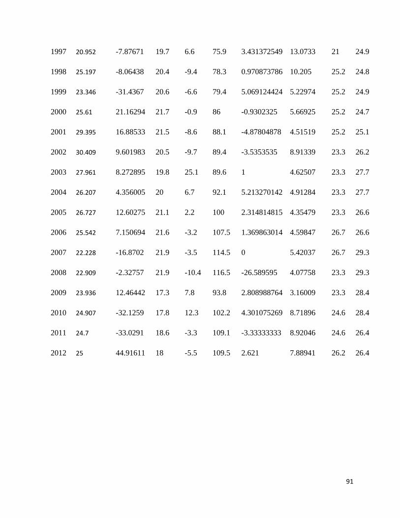
91
1997 20.952 -7.87671 19.7 6.6 75.9 3.431372549 13.0733 21 24.9
1998 25.197 -8.06438 20.4 -9.4 78.3 0.970873786 10.205 25.2 24.8
1999 23.346 -31.4367 20.6 -6.6 79.4 5.069124424 5.22974 25.2 24.9
2000 25.61 21.16294 21.7 -0.9 86 -0.9302325 5.66925 25.2 24.7
2001 29.395 16.88533 21.5 -8.6 88.1 -4.87804878 4.51519 25.2 25.1
2002 30.409 9.601983 20.5 -9.7 89.4 -3.5353535 8.91339 23.3 26.2
2003 27.961 8.272895 19.8 25.1 89.6 1 4.62507 23.3 27.7
2004 26.207 4.356005 20 6.7 92.1 5.213270142 4.91284 23.3 27.7
2005 26.727 12.60275 21.1 2.2 100 2.314814815 4.35479 23.3 26.6
2006 25.542 7.150694 21.6 -3.2 107.5 1.369863014 4.59847 26.7 26.6
2007 22.228 -16.8702 21.9 -3.5 114.5 0 5.42037 26.7 29.3
2008 22.909 -2.32757 21.9 -10.4 116.5 -26.589595 4.07758 23.3 29.3
2009 23.936 12.46442 17.3 7.8 93.8 2.808988764 3.16009 23.3 28.4
2010 24.907 -32.1259 17.8 12.3 102.2 4.301075269 8.71896 24.6 28.4
2011 24.7 -33.0291 18.6 -3.3 109.1 -3.33333333 8.92046 24.6 26.4
2012 25 44.91611 18 -5.5 109.5 2.621 7.88941 26.2 26.4
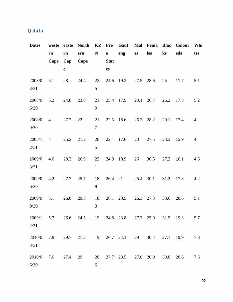
92
Q data
Dates weste
rn
Cape
easte
rn
Cap
e
North
ern
Cape
KZ
N
Fre
e
Stat
es
Gaut
eng
Mal
es
Fema
les
Blac
ks
Colour
eds
Whi
tes
2008/0
3/31
5.1 28 24.4 22.
5
24.6 19.2 27.5 28.6 25 17.7 5.1
2008/0
6/30
5.2 24.8 23.8 21.
9
25.4 17.9 23.1 26.7 26.2 17.8 5.2
2008/0
9/30
4 27.2 22 21.
7
22.5 18.6 26.3 28.2 29.1 17.4 4
2008/1
2/31
4 25.2 21.2 20.
5
22 17.6 23 27.5 23.3 15.9 4
2009/0
3/31
4.6 28.3 26.9 22.
1
24.8 18.9 26 30.6 27.2 16.1 4.6
2009/0
6/30
4.2 27.7 25.7 18.
9
26.4 21 25.4 30.1 31.2 17.8 4.2
2009/0
9/30
5.1 26.8 29.3 18.
3
28.1 23.5 26.3 27.3 33.6 20.6 5.1
2009/1
2/31
5.7 26.6 24.5 19 24.8 23.8 27.3 25.9 31.5 19.3 5.7
2010/0
3/31
7.8 29.7 27.2 19.
1
26.7 24.1 29 30.4 27.1 19.9 7.8
2010/0
6/30
7.6 27.4 29 20.
6
27.7 23.5 27.8 26.9 30.8 20.6 7.6

93
2010/0
9/30
6.9 26.7 25.3 19.
5
29.7 23.9 25.1 28.4 33.9 21.8 6.9
2010/1
2/31
5.6 24.2 24.3 19.
4
27.1 23.7 24.4 24.1 32.5 21.3 5.6
2011/0
3/31
5.6 26.7 31.1 19.
8
27.9 23.3 27 26.4 31.2 22.1 5.6
2011/0
6/30
4.2 28.4 28.4 20 28 25.2 26.6 30.3 32.2 20.9 4.2
2011/0
9/30
5.5 26.8 28 18.
7
25 25.6 25.8 27.8 31.4 24.1 5.5
2011/1
2/31
6 26.9 26.4 18.
8
29.2 23.1 25.4 28.5 30.6 20.8 6
2012/0
3/31
5.3 28 25.3 20 31.9 23.2 26.6 29.4 32 23.1 5.3
2012/0
6/30
7 28.5 29.9 19.
3
32.7 23.7 27.6 29.4 32.4 22 7
2012/0
9/30
6.5 28.8 29.6 20.
6
31.6 22 28.7 28.9 34.7 24.3 6.5
2012/1
2/31
4.8 29.5 28.3 21.
9
32.7 21.2 27.3 31.9 32.8 23.6 4.8
2013/0
3/31
7.1 29.8 29.3 20.
5
31.2 23.2 29.7 30 32 22.9 7.1
2013/0
6/30
5.4 30.2 29.5 22.
2
32.8 22.1 30.6 29.7 33.3 24.1 5.4

94
2013/0
9/30
5 30.4 27.9 20.
6
33.7 22.1 31.2 29.5 32.7 23.6 5
2013/1
2/31
6.5 27.8 24.9 19.
9
33 22.4 27.5 28.2 30.4 20.8 6.5
2014/0
3/31
7.1 29.4 29 20.
7
34.7 23.6 30 28.8 31 19.8 7.1
2014/0
6/30
6.6 30.4 32.3 23.
7
35 22.2 30 30.8 31.3 24.1 6.6
2014/0
9/30
7.5 29.5 29.7 24.
1
34.6 21.5 31.1 27.7 33.6 23.1 7.5
2014/1
2/31
6 29.1 28.7 20.
8
32.2 21.8 30.9 27.2 33.2 22.1 6

95
APPENDIX 2: JOHANSEN COINTEGRATION TESTS RESULTS
Unrestricted Cointegration Rank Test (Trace)
Hypothesized Trace 0.05
No. of CE(s) Eigenvalue Statistic Critical Value Prob.**
None * 0.950448 209.5272 125.6154 0.0000
At most 1 * 0.841479 122.3899 95.75366 0.0002
At most 2 0.733420 68.97573 69.81889 0.0582
At most 3 0.419718 30.63534 47.85613 0.6860
At most 4 0.298648 14.85237 29.79707 0.7896
At most 5 0.121453 4.564766 15.49471 0.8532
At most 6 0.027534 0.809675 3.841466 0.3682
Trace test indicates 2 cointegrating eqn(s) at the 0.05 level
* denotes rejection of the hypothesis at the 0.05 level
**MacKinnon-Haug-Michelis (1999) p-values
Unrestricted Cointegration Rank Test (Maximum Eigenvalue)
Hypothesized Max-Eigen 0.05
No. of CE(s) Eigenvalue Statistic Critical Value Prob.**
None * 0.950448 87.13732 46.23142 0.0000
At most 1 * 0.841479 53.41413 40.07757 0.0009
At most 2 * 0.733420 38.34039 33.87687 0.0137
At most 3 0.419718 15.78297 27.58434 0.6841
At most 4 0.298648 10.28760 21.13162 0.7172
At most 5 0.121453 3.755091 14.26460 0.8842
At most 6 0.027534 0.809675 3.841466 0.3682

96
Max-eigenvalue test indicates 3 cointegrating eqn(s) at the 0.05 level
* denotes rejection of the hypothesis at the 0.05 level
**MacKinnon-Haug-Michelis (1999) p-values
Lag length
Lag LogL LR FPE AIC SC HQ
0 -622.7142 NA 1.71e+10 43.42857 43.75860 43.53193
1 -477.1712 210.7864 24348706 36.77043 39.41072* 37.59734
2 -406.4062 68.32485* 10625851* 35.26939* 40.21995 36.81984*
* indicates lag order selected by the criterion
LR: sequential modified LR test statistic (each test at 5% level)
FPE: Final prediction error
AIC: Akaike information criterion
SC: Schwarz information criterion
HQ: Hannan-Quinn information criterion
Choosing the appropriate model
Selected (0.05 level*) Number of Cointegrating Relations by Model
Data Trend: None None Linear Linear Quadratic
Test Type No Intercept Intercept Intercept Intercept Intercept
No Trend No Trend No Trend Trend Trend

97
Trace 2 3 2 3 3
Max-Eig 2 3 3 3 3
*Critical values based on MacKinnon-Haug-Michelis (1999)
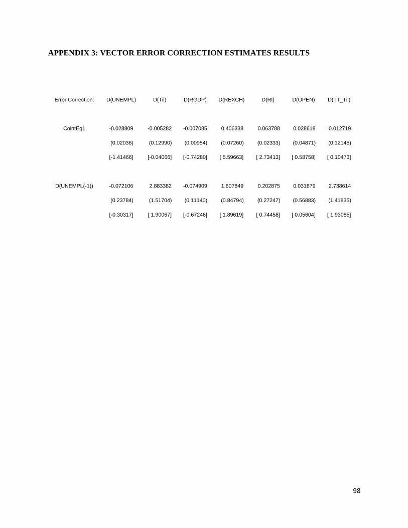
98
APPENDIX 3: VECTOR ERROR CORRECTION ESTIMATES RESULTS
Error Correction: D(UNEMPL) D(Tii) D(RGDP) D(REXCH) D(RI) D(OPEN) D(TT_Tii)
CointEq1 -0.028809 -0.005282 -0.007085 0.406338 0.063788 0.028618 0.012719
(0.02036) (0.12990) (0.00954) (0.07260) (0.02333) (0.04871) (0.12145)
[-1.41466] [-0.04066] [-0.74280] [ 5.59663] [ 2.73413] [ 0.58758] [ 0.10473]
D(UNEMPL(-1)) -0.072106 2.883382 -0.074909 1.607849 0.202875 0.031879 2.738614
(0.23784) (1.51704) (0.11140) (0.84794) (0.27247) (0.56883) (1.41835)
[-0.30317] [ 1.90067] [-0.67246] [ 1.89619] [ 0.74458] [ 0.05604] [ 1.93085]