THE IMPACT OF THE INCREASE IN SMALL SATELLITE LAUNCH TRAFFIC ON THELONG-TERM EVOLUTION OF THE SPACE DEBRIS ENVIRONMENT

Jonas Radtke(1), Enrico Stoll(1), Hugh Lewis(2), and Benjamin Bastida Virgili(3)

(1)Technische Universitaet Braunschweig, Institute of Space Systems, Braunschweig, Germany, Email: {j.radtke,e.stoll}@tu-braunschweig.de

(2)Astronautics Research Group, University of Southampton, Southampton SO17 1BJ, UK, Email: h.g.lewis@soton.ac.uk(3)IMS Space Consultancy @ ESA/ESOC Space Debris Office (OPS-GR), Robert-Bosch-Str. 5, DE-64293 Darmstadt,

Germany, Email: Benjamin.Bastida.Virgili@esa.int

ABSTRACT

In recent years, the launch traffic to low Earth orbits(LEO) has undergone a significant change: while inthe beginning of this century the launch rates droppedto their lowest level since the beginning of the spaceage, the yearly number of launches performed has nowrecovered to 20th century levels. Although absolutelaunch numbers are now comparable to historic levels,fundamental space activity has changed dramatically:instead of launching few, complex, large and expensivespacecraft, as done typically by governments, the trendis now towards the deployment of space systems that aremuch smaller, less complex and of lower cost. A majorfactor in this change of philosophy has been the shiftfrom institutional operators towards those from privateindustries. Current market analyses furthermore assumethat these recent changes in launch traffic are only thebeginning of a continuing change in the use of LEO.

When considering this shift towards increasing numbersof smaller satellites, the question arises what impactwill these objects have on the long-term evolutionof the space debris environment? A general concernexists that small satellites might pose a major threat toclassical missions, as many of them are not equippedwith propulsion systems and thus cannot perform anycollision avoidance or end-of-life disposal manoeuvres.To assess the role of these small satellite missions inthe evolution of the space debris environment, long-term projections of the space debris environment fordifferent assumptions of small satellites’ launch rates,release orbits and capabilities have been performedand their results are presented in this paper. For theseprojections, the Institute of Space System’s tool LUCA(Long Term Utility for Collision Analysis) has been used.

In this paper, the current trends in launch traffic are firstsummarized, focusing on describing the characteristicsof small satellites. Following this, an approach to projectfuture launch traffic scenarios using knowledge from

currently launched small satellites is described. Thisapproach is based on deriving distributions that capturethe characteristics of current small satellites missions,such as their mass, shape, release orbit, launcher, etc.Depending on the scenario to be simulated, these dis-tributions are manipulated and to-be-launched objectsdrawn from them during the simulations. This methodis applied to different parametric variations of the smallsatellite launch traffic, including the number of objectsto be launched, their orbital distribution, their potentialto perform post-mission disposal and collision avoidancemanoeuvres, and their launch as swarms of satellites.

Key words: Long-term evolution; small satellites; newspace; LUCA;.

1. INTRODUCTION

In recent years, launch traffic to low Earth orbits (LEO)has undergone enormous changes. Alongside a generalrecovery of the launch rate, which dropped to an all-timelow in the beginning of this century (cf. Figure 1), thenumber of launched small satellites and their share inall launched objects has increased significantly. In thispaper, the term small satellites is used for all payloadswith masses below 100 kg. The reason for this changeis probably a combination of several factors, such asthe general miniaturization of satellite parts and theirstandardization, new, and supposably cheaper launchopportunities such as the Indian PSLV or upcominglaunchers such as Virign’s LauncherOne or RocketLab’s Electron, alongside with America’s legalizationof private spaceflight in 2004 [1]. These factors arefurthermore enhanced by newly emerging markets fromincreased worldwide connectivity and computationcapabilities, allowing easy and automated processing ofthe vast amounts of data collected by the small satellites.While the underlying reasons of this shift shall not bediscussed in detail in this paper, questions of ”‘if”’ and”‘how”’ the increase of launched payloads, although

Proc. 7th European Conference on Space Debris, Darmstadt, Germany, 18–21 April 2017, published by the ESA Space Debris Office

Ed. T. Flohrer & F. Schmitz, (http://spacedebris2017.sdo.esoc.esa.int, June 2017)

small and of low masses, might affect the long-termevolution of the space debris environment are important.This is vital to be able to judge on the applicability ofexisting space debris mitigation guidelines and standardsfor small satellites.

Some work on this topic has already been published [2],[3], [4], [5]. In these studies, different projections forpossible future CubeSat or small satellite traffic weredesigned and the impact of this traffic on the spacedebris environment analysed. All publications agreethat, if current trends in small satellite traffic continue orare even surpassed, small satellites will pose a possiblethreat to the space debris environment. This papercomplements the previous work by designing differentsmall satellite traffic scenarios, and additionally varyingcharacteristics, and capabilities of small satellites ina parametric manner. All performed variations aresummarized in Table 1. Some early results on smallsatellites’ impact on the space debris environment fromthe same study were already published in [5].

2. TRENDS IN CURRENT LAUNCH TRAFFIC

The evolution of both the number of launched objects aswell as their relative share in all launches for differentmass classes of satellites is shown in Figure 1. From thisfigure, two trends become apparent: first of all, the totalnumber of launched objects has been increasing since thevery low numbers encountered in the first decade of the21st century, which is valid for all masses of objects. Sec-ond, both in terms of total number of objects but also theirrelative share in all objects, small satellites with massesbelow 100 kg have encountered the largest increase, lead-ing to at least 100 objects launched per year since 2012and a share well above 50%.

Figure 1. Histogram of number of launches per mass binfor years 2005 to 2015 and share of small satellites inoverall launch rates. Data from Discos.

Besides the number of objects, their distributions of or-bital parameters, mass, area-to-mass ratios etc. are also

of high interest for a launch traffic creation. To gather thisinformation, a compilation of databases from the Univer-sity of Southampton [2] and TU Berlin [6] was used, andpartially updated when information on objects was miss-ing. Due to availability of the data at the time the analyseswere performed, only small satellites launched betweenJanuary 2012 and May 2015 were considered.

3. LONG-TERM SCENARIOS

To be able to estimate the impact of the increasing num-ber of small satellites, a set of future launch traffic sce-nario was defined, on which basis characteristics and ca-pabilities of small satellite launches were varied para-metrically. These scenarios were then used to projectthe long-term evolution of the space debris environment.Simulations shown in this paper were performed usingthe long-term evolution tool LUCA (Long term utilityfor collision analysis) [7]. The results of the simula-tions were then compared against a reference scenario, inwhich no additional small satellite launches were consid-ered. In the following, the different scenarios are gener-ally described, a detailed description of the small satellitelaunch traffic is given in Section 4.

The reference scenario was chosen to be in-line withcurrent simulations performed by the Inter-AgencySpace Debris Coordination Committee (IADC) andthose for other publications, such as those in [9]. Theinitial population used for the simulations includedall LEO-crossing objects ≥ 10 cm on January 1st

2013, derived from ESA’s Meteoroid and Space DebrisTerrestrial Environment Reference Model (MASTER)[10], [11]. The traffic was created by repeating all LEOand geostationary transfer orbit (GTO) launches between2005 and 2012. It was assumed that no further explosionsoccur and that 90% of all spacecraft and rocket bodiesperform a disposal to an eccentric 25-year orbit at the endof their active mission, if their orbital lifetime exceedsthis limit. Note that this assumption for post-missiondisposal is rather optimistic compared to results fromrecent studies, which show that only about 20% of allspace systems, which are not naturally compliant, meeta 25-year disposal rule [12], [13]. For the future solaractivity, five different random-cycles were created. Allsimulations were performed for simulation time framesof 200 years, performing 50 Monte-Carlo runs perscenario.

Atop this reference scenario, different assumptions forfuture small satellite traffic were assumed. The completesimulation plan is shown in Table 1. For the sake of clar-ity, scenario 1.a.2 is from hereon denoted as small satel-lite baseline scenario. If not stated otherwise, all varia-tions are performed in reference to this scenario.

Table 1. Simulation plan of long-term scenarios includ-ing small satellites. SMA stands for semimajor axis,PMD for post-mission disposal.

Scen. Number Short description VariationRef Reference scenario -1.a.1 Low small sat. traffic Assume a low, constant small

sat. launch rate1.a.2 Medium small sat. traffic Assume a medium small sat.

launch rate1.a.3 High small sat. traffic Assume a high small sat. launch

rate1.b.1 Increase CubeSat form factor 1U to 3U, 3U to 6U1.b.2 Increase CubeSat form factor 1U to 6U, 3U to 12U1.b.3 Increase CubeSat form factor 1U to 12U, 3U to 24U1.c.1 Assume low small sat. launch

altitudeLaunch small satellites 50\50 toSMA bins 2 and 3 from Table 3

1.c.2 As 1.c.1, increase piggy backrate

As 1.c.1, 80% piggy backlaunched

1.c.3 Assume high small sat. launchaltitude

Launch small satellites to SMAbins 3 (25%), 4 (50%), and 5(25%) from Table 3

1.c.4 As 1.c.3, increase piggy backrate

As 1.c.3, 80% piggy backlaunched

1.d.1.i-iii Some small sats. are launchedin swarms

launch 20% of small sats inswarms of [10 - 30; 30 - 50; 50- 80] sats.

1.d.1.iv-vi Half of all small sats. arelaunched in swarms

launch 50% of small sats inswarms of [10 - 30; 30 - 50; 50- 80] sats.

1.d.1.vii-ix Most small sats. are launched inswarms

launch 80% of small sats inswarms of [10 - 30; 30 - 50; 50- 80] sats.

2.a.1.i-iii∗ Small sats perform PMD to 25year orbits

[30%; 60%; 90%] PMD suc-cess; eccentric 25 year PMD or-bits.

2.a.1.iv-vi∗ Small sats perform PMD to 10year orbits

[30%; 60%; 90%] PMD suc-cess; eccentric 10 year PMD or-bits.

2.a.1.vii-ix∗ Small sats perform PMD to 5year orbits

[30%; 60%; 90%] PMD suc-cess; eccentric 5 year PMD or-bits.

2.a.2.i-iv∗ Small satellites perform colli-sion avoidance

[30%; 70%; 90%; 100%] colli-sion avoidance success.

∗Small satellites are assumed to have active lifetimes of five years.

4. CREATION OF FUTURE LAUNCH TRAFFIC

To perform the long-term simulations, most crucial isthe creation of traffic for future launches. As the sce-narios shall be comparable against each other, and es-pecially also against the reference scenario, the under-lying assumptions for launched objects need to be con-sistent. Therefore, the launch traffic creation is based onderiving distribution functions from prior launched smallsatellites and randomly drawing objects from these dis-tributions. For background objects, random objects weredrawn from the repeating launch cycle. To launch ob-jects during the simulations, the following parameters areneeded:

• total number of payloads to be launched,

• orbital parameters,

• satellite characteristics such as mass and cross-section,

• number of objects included in a single launch,

• used launcher system,

• insertion of mission related objects (MRO) duringthe launch,

• capabilities of the launched objects such as post-mission disposal and collision avoidance.

4.1. Number of payloads to be launched

The numbers of launched background objects and smallsatellites were derived differently. To be in-line with thereference scenario, the number of launched backgroundobjects is a repeating cycle, based on launches performedbetween 2005 and 2012. For the small satellite launchrates, three different scenarios were assumed: One con-stant scenario, one medium launch rate scenario, and onehigh launch rate scenario. For the constant launch ratescenario, it was assumed that the number of small satel-lites stays about the same as in 2013, thus 100 objectsper year were included. Similar to [2], the number ofsmall satellites launched per year during the other sce-narios were estimated using different Gompertz Logisticcurves:

L = bae−bec(t−t0)

+ 0.5c. (1)

The coefficients used for the different scenarios areshown in Table 2; Figure 2 shows the numbers of pay-loads launched during the different scenarios, includingthe historical rate for small satellites..

Table 2. Gompertz coefficients used in the logistic func-tions to determine number of launched small satellitesduring long-term simulations.

Coefficient Medium Higha 270 540b 5 21.5c 0.15 0.235t0 2003 2003

Figure 2. Launch rate of small satellites and backgroundpayloads for different future scenarios.

4.2. Orbital parameters of payloads

Second, the orbital parameters for each launch includingsmall satellites needed to be determined. To achieve this,orbital parameters of past launches have been analysed,from which distributions of the orbital parameters werederived. To create the launch traffic scenarios, the orbitalparameters were then drawn from these distributions.The distributions have only been derived for smallsatellites, background objects were randomly drawnfrom the objects in the repeating launch cycle.

The basis for the small satellite launches is the semi-major axis. From the distribution of past small satel-lite launches, a Gaussian mixture with five componentswas derived. It was decided to use a Gaussian mixturefor three reasons: First of all, it was assumed that smallsatellites will be launched in the futures to similar re-gions of interest as today, but not to identical orbits. Us-ing a parametric distributions offers an easy solution toadd a spread to the orbital parameters. Secondly, fromanalysis of past launches, different altitude regions of in-terest were identified: launches directly from the ISS,two peaks in semimajor axes around 7000 km and 7200km, some launches between the ISS orbit and 7000 km,and last very some launches to high orbits above 7200km. Third, in the progress of the study, variations of thelaunch altitudes were to be performed. Using the deriveddistributions, this aim can simply be achieved by adopt-

Table 3. Components of the Gaussian mixture distribu-tion to draw the semimajor axis for small satellite pay-loads. For scenarios 1.c.x, the mixing coefficients havebeen varied accordingly.

Class Mix. Coeff. µ / km σ / kmSMA 1 0.3075 6547.5 20.47SMA 2 0.1139 6751.7 63.14SMA 3 0.4191 7045.8 45.57SMA 4 0.1503 7171.9 39.69SMA 5 0.0091 7787.4 141.85

ing the mixing coefficients. The resulting distributionstogether with the histogram of launched small satellitesare shown in Figure 3. The expected values, standard de-viations and mixing coefficients for the distributions areshown in Table 3.

Figure 3. Gaussian mixture distribution to determine fu-ture small satellite launches together with the histogramof semimajor axis from launched small satellites. For thehistogram, 120 bins have been used.

The second orbital parameter needed is the eccentricity.Here it was found that so far, all small satellites wereplaced on near-circular orbits, random values from alog-normal distribution with a mean of −6.39 and astandard deviation of 1.3 were drawn. In accordancewith the available data, only eccentricities above 0 andbelow 0.08 were accepted.

The third orbital parameter used is the inclination. Again,a Gaussian mixture model was derived for their distribu-tion, but as the inclinations used depend on the semima-jor axes, one model was derived for each semimajor axisclass. The resulting components are shown in Table 4, thedistribution together with a histogram of the inclinationsfrom small satellites launches are shown exemplary forsemimajor axis class three in Figure 4. For those classesof the mixture functions that were identified to representsun-synchronous objects, the inclinations were not deter-mined by a random draw from the distribution, but using

Table 4. Components of the Gaussian mixture distribu-tions to draw the inclination for small satellite payloads.

Class Mix. Coeff. µ / ◦ σ / ◦

1, 1 0.2593 37.0466 7.35851, 2 0.6074 51.6151 0.02351, 3 0.1111 67.0353 2.28701, 4 0.0222 SSO -2, 1 0.44 39.2659 1.53642, 2 0.4 51.638 0.00412, 3 0.16 SSO -3, 1 0.1196 65.2630 1.81823, 2 0.8151 SSO -3, 3 0.0652 120.4981 0.00014, 1 0.0455 19.9633 0.00584, 2 0.3636 45.0158 0.01324, 3 0.1667 76.46 5.40264, 4 0.4242 SSO -5, 1 0.5 82.485 0.02125, 2 0.5 SSO -

the simplified formulation for sun-synchronous inclina-tions:

isso = acos(−0.09896 · a

RE·(1− e2

)). (2)

Here, a is the semimajor axis of the orbits,RE the Earth’sradius and e the eccentricity.

Figure 4. Gaussian mixture distribution to determine fu-ture small satellite launches together with the histogramof inclinations from launched small satellites of semima-jor axis class 3. For the histogram, 75 bins have beenused.

Figure 5 shows the orbits of 10000 small satellites drawnfrom the distribution functions together with those fromthe underlying databases. It can be seen that the “hotspots” are well reproduced using the distributions. Due tousing normal distribution functions and the large numberof objects, the spread around these areas are enlarged.

Figure 5. Inclination over semimajor axis for small satel-lites from databases (red) and drawn from derived distri-butions (green). 10000 random draws.

As all objects were placed on near-circular orbits, the ar-gument of perigee is of less interest, so it was set on arandom value between 0◦ and 360◦. Furthermore, theright ascension of ascending node (RAAN) and meananomaly are randomized during the collision rate deter-mination algorithms used. Therefore, these two valuesare randomly set between 0◦ and 360◦. Note that thisprocedure was different for those scenarios in which asubset of the small satellites was launched within swarms(refer to Section 4.7).

4.3. Satellite characteristics

For the long-term simulations, the satellites’ characteris-tics are described using the mass and diameter. For thelaunch traffic creation it was decided to use the mass asindependent variable and a double-logarithmic fit to de-termine the diameter based on the mass. For CubeSats, adifferent approach was used.

The mass of the to-be-launched small satellite was sim-ply determined by randomly drawing from all satelliteswithin the used databases. Then, based on the mass, a fitover all available satellite masses and diameters was usedto determine the diameter:

d = 10−0.8877 ·m0.4523. (3)

To account for variations within the densities of typicalsatellites, a random variation of ±50% of the diameterwas allowed. To determine the cross sections (and thusthe area-to-mass ratios important for the propagation), allsmall satellites were assumed to be spherical. As thisestimation does not work out well for very light-weightsatellites, which typically are CubeSats. In the database,CubeSats are mostly 1U, 2U or 3U satellites. Therefore,objects with masses according to the CubeSat standardwere assumed to be CubeSats. The cross sections of theseCubeSats were determined using the tool CROC from

Table 5. characteristics of CubeSats during the simula-tions. Note that CubeSats larger than 3U were only con-sidered during simulations 1.b.x.

Type Mass / kg Diameter / m Cross-Section / m2

1U 1.333 0.1377 0.01492U 2.666 0.1884 0.02793U 4.0 0.2224 0.03886U 12.0 0.2642 0.054812U 24.0 0.3186 0.079724U 48.0 0.4061 0.1295

ESA’s DRAMA Tool Suite [8]. Their values are statedin Table 5. Note that CubeSats larger than 3U were onlyused in simulations 1.b.x.

4.4. Number of objects per launch

Next to payloads, the number of rocket bodies injectedalso have a large impact on the long-term evolution ofthe space debris environment, so the number of objectsthat are launched together need to be considered. To de-termine this number, the launches are distinguished be-tween background launches, piggy-back and dedicatedsmall satellite launches. In case of piggy-back launches,the small satellites are released into orbit together with agenerally larger background object.

For the number of background objects per launch, the re-peating launch cycle was used. The launches included inthere could be fitted using a log-normal distribution withµ = 0.4171 and σ = 0.67. A maximum number of eightbackground objects per launch were allowed.

To determine the number of piggy-back objects in onelaunch, the number of small satellites per launch vehiclelaunched between 2012 and 2015 have been used. Thesemove between 1 and 12 objects per launch, with the ex-ception of US military missions with more than 25 ob-jects per launch. Additionally, almost 80 small satelliteswere launched from the ISS. For the launch traffic cre-ation, the latter ones have been assumed to be exceptionalevents, and a normal logarithmic distribution function hasbeen used to describe the number of small satellite inpiggy-back launches with µ = 0.8869 and σ = 1.0346.

To determine the number of small satellites in dedicatedlaunches, a log-normal distribution with µ = 1.2653 andσ = 1.10551 was used.

If not stated otherwise, it was assumed that 50% of thesmall satellites were launched as piggy back objects withbackground objects.

4.5. Used launcher system

For the launch system used, all launches included in therepeating launch cycle were analysed in regards to theirmass delivered to orbit. Based on the mass to be deliv-ered to orbit in the long-term simulation, an appropriatesystem was randomly chosen from those used in the re-peating launch cycle.

In addition to the rocket bodies from launch to LEO, alsorocket bodies to GTOs were also considered in the sim-ulations. As these are not correlated with any missionwithin this study, the GTO rocket bodies were includedbased on the launches in the repeating background launchcycle.

4.6. Insertion of mission related objects

From the launches performed between 2005 and 2012 itwas found that 28% of all LEO missions released at leastone mission related object (MRO) into orbit that lasted atleast three months. Furthermore 73% of all GTO rocketbodies released at least one, in general very large, missionrelated object. Therefore, for both types of launches, ran-domly chosen mission related objects were released intoclose vicinity of the launch orbit.

4.7. Launching swarms of satellites

In one of the scenarios, different shares of all smallsatellites were assumed to be launched in swarms ofsatellites of different sizes. As swarms of satellites,three different types were assumed possible: stringsof pearl, Walker-Delta constellations, and Walker-Starconstellations.

In the process, at first the number of objects in the swarmto be created is determined by a random draw from anuniform distribution of even numbers. Second, it is de-cided if the swarm was a string of pearl or any type ofconstellation. No data is available to indicate a correla-tion between number of objects in a swarm of satellitesand type of swarm, as the underlying assumption is thatstrings of pearls tend to be smaller than other types ofconstellations. To apply this assumption, a normal distri-bution of the shape

pc =1

2

(1 + erf

(nsats − µ√

2σ2

))(4)

is used. Here, the mean value is decribed by µ = 25and the standard deviation with σ = 10. For a swarmconsisting of nsats members, the probability of being aconstellation pc is determined. Then, this probability iscompared against a random number z from a uniformdistribution in the interval [0, 1[. If z ≤ pc, the swarmis assumed to be a constellation, else it is considered

as a string of pearls. Furthermore is decided if theconstellation is Walker-Star or Walker-Delta. Again, nodata is available to support this decision, therefore it wasassumed that highly inclined constellations are generallyWalker-Star, others are Walker-Delta. To decide betweenthose two types, again a normal distribution was used,with the inclination being the independent variable,µ = 80◦ and σ = 2◦. If the inclination exceeds 90◦,180◦ − i is used. The resulting value is used as probabil-ity, if a constellation is a Walker-Star constellation.

Next, the distribution of the objects along their orbitalplanes is determined. For strings of pearls, the approachis straight forward, as all object are on a single orbitalplane. This plane is randomly drawn, the objects arethen evenly distributed in slots along this plane. Forthe constellations, first the number of planes are deter-mined, which are randomly chosen to be between threeand eight. Second, the nodes of the single planes areset. For Walker-Delta constellations, they are evenly dis-tributed along 360◦, for Walker-Star constellations along180◦. Last, the objects are evenly distributed in slotsalong each plane. For Walker-Delta constellations, theoffset between slots in neighbouring planes is defined bythe Walker factor as:

w =2π

nsats,plane· 1

nplanes. (5)

For Walker-Star constellations, the slots are also evenlydistributed along the orbital planes, with the offsetbetween neighboring planes being half the difference ofobjects in a single plane.

5. RESULTS OF THE LONG-TERM SIMULA-TIONS

5.1. Reference and baseline scenarios

All simulations were analysed in comparison to areference scenario, in which no extra small satelliteswere included (only those included in the repeatinglaunch cycle were considered). The main results ofthis simulation are shown in Figure 6. The simulationprojects a constant median number of objects, with theworst case being an increase of about 65% and a bestcase a decrease to about 73% of the initial number ofobjects in orbit. On the median, during the first half ofthe simulation, 0.17 catastrophic collisions are triggeredper year, afterwards the collision rate decreases to 0.13per year. In between, the collision rate undergoes asubtle change. Considering these numbers it has to bekept in mind that the chosen scenario has, comparedwith most periods of spaceflight, a very low launchtraffic. Furthermore, the results are highly sensitive toimplementations of underlying models and assumptionssuch as future solar activity.

The scenario in which a medium launch rate of smallsatellites is superimposed to the traffic of background ob-jects is chosen as the small satellite baseline scenario.The results of this scenario are also shown in Figure 6. Inthis scenario, the additional launch traffic leads to a directincrease of the number of objects in LEO by about 70%during the first half of the simulation. From then, only alow further increase by less than 10% on the median overthe rest of simulation time frame can be observed. Thenumber of catastrophic collisions evolves similar to thatof the reference scenario, but at different rates. Again,after about half of the simulation time frame, the rate de-creases again. Until then, 0.31 collisions are trigged peryear. For the rest of the simulation time, on the median0.25 collision occur per year. Both rates behave very lin-ear over the stated time frames (with correlation coeffi-cients of R2 = 0.99 between the correlation rates andtheir linear trends).

To determine the statistical significance of the differencein the median of two long-term simulations, the results interms of numbers of objects in the environment have beenanalysed using a Wilcoxon rank sum test [14]. This is anon-parametric hypothesis test using as null-hypothesisthat the medians of the tested samples from independentpopulations are identical at an assumed significance level(α). As result, the test returns a p-value, which describesthe probability that the tested samples come fromdistributions which fulfill the null-hypothesis. If p < α,the null-hypothesis is rejected, indicating a significantdifference in the medians of the tested simulations. Thestandard significance level for this test is α = 0.05,which has also been used in the context of the paper.With this test, always two long-term scenarios, whichdiffer in one parameter of the simulation set-up werecompared. If the null-hypothesis hypothesis is rejectedwith this test, the influence of the changed parameter hada significant impact on the median results.

While the difference between reference and baseline sce-nario appears obvious already from the graphical com-parison, differences were less obvious when consideringother scenarios. Comparing these two scenario, using theWilcoxon rank sum test, the null-hypothesis is rejectedat the 5% significance level over the complete simulationtime frame.

5.2. Variation of the small satellite launch trafficrate (scenarios 1.a.x)

The first variation of the small satellite launch trafficwas with respect to the number of objects includedinto the population. The results of the variations areshown together with the reference and baseline scenariosin Figure 7. Note that the spread in the simulationresults of the baseline and high launch traffic scenario areomitted for clarity, but exist in all results in similar extent.

Scenario 1.a.1 has the lowest number of added small

Figure 6. Results of the baseline scenario considering a medium small satellite launch rate. Shown are median (thick line)and 10% and 90% quantiles (thin lines). Left: Effective number of objects in LEO over time, right: Cumulated numberof catastrophic collisions. Computed from 50 Monte-Carlo runs.

satellites. The median number of objects increases by26% and behaves in an almost linear fashion. The num-ber of catastrophic collisions increases strongly duringthe first half of the simulation with 0.22 median collisionsper year, followed by 0.18 collisions per year. Again,the cumulative number of collisions behaves linear dur-ing both time frames (R2 = 0.99). In the scenario with ahigh small satellite traffic, the median number of objectsincreases by about 80% until the year 2060, followed bya less strong increase over the remaining 150 years ofsimulations leading to a total increase of 135%. In con-trast to the other scenarios, the number of catastrophiccollision increases almost linearly with 0.43 collisionsper year (R2 = 0.99) over the complete simulation timeframe.

Again, the difference of the scenarios with respect tothe reference scenario, but also against one another hasbeen tested using the rank sum test. Even though thespreads within the simulation results overlap, especiallyfor the reference scenario and case 1.a.1 (constant launchrate), the null-hypothesis is rejected over the completesimulation time frame for all scenarios when comparedagainst the reference case. Comparing the small satellitescenarios against one another, a significant differenceis achieved after 15 years when comparing the baselinescenario and scenario 1.a.1 (constant launch rate) andalready after five years when comparing either of thescenarios against scenario 1.a.3 (high launch rate). Whilethis result is not surprising for the small satellite baselinecase and scenario 1.a.3 (high launch rate), it shows thatalready the small satellite launch traffic as performedtoday, which is represented by scenario 1.a.1 (constantlaunch rate), has already a significant impact on the longterm evolution of the space debris environment.

5.3. Variation of the small satellite form factor (sce-narios 1.b.x)

The second variation was a change in the form factorof all launched CubeSats. The variation has beenperformed under the assumption that CubeSat sizes willincrease in the future to enable more capable payloadsfor commercial missions. Three variations as shown inTable 1 were performed with CubeSat characteristics(mass and cross section) as stated in Table 5. The resultsof these simulations are shown in Figure 8.

In terms of the median number of objects in the environ-ment, during the first about eighty years, all simulationsbehave similarly, leading to an increase in the number ofobjects between about 60% (for the baseline scenario andscenario 1.b.1) and 75% (for scenarios 1.b.2 and 1.b.3).Over the time, the results start to differ and the increaserelaxes in all cases, but while for the baseline case thenumber of objects stays almost constant for the remain-ing simulation time frame, it further increases for the sce-narios with the variations. This leads to a total increaseof about 75% in scenario 1.b.1, 100% in scenario 1.b.2,and even 110% in scenario 1.b.3. A similar behaviour isshown for the number of catastrophic collisions: whileduring the first half of the simulation all small satellitescenario show a median of about 0.31 collisions per year,the numbers start differing between scenarios afterwards.For the baseline scenario, the rate decreases to 0.25 col-lisions per year, for scenario 1.b.1 it stays around 0.31,and for scenarios 1.b.2 and 1.b.3 it increases to 0.34, andeven 0.47 during the last 50 years of the simulation timeframe. Therefore, in terms of collisions, the scenarios inwhich the CubeSats sizes are increased, an accelerationin the collision activities can be observed.

In terms of the statistical significance of the results,the null-hypothesis is rejected when comparing thevariations against the baseline scenario at the end ofthe simulation time frame. For the first 40 years nev-

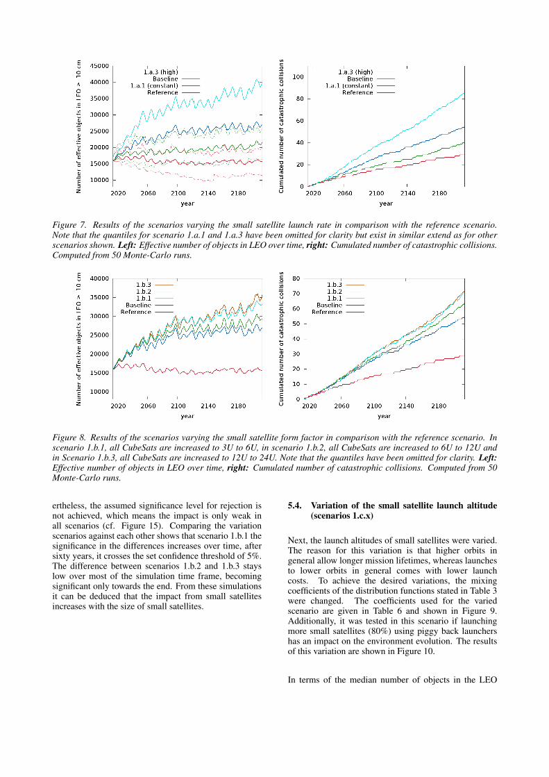
Figure 7. Results of the scenarios varying the small satellite launch rate in comparison with the reference scenario.Note that the quantiles for scenario 1.a.1 and 1.a.3 have been omitted for clarity but exist in similar extend as for otherscenarios shown. Left: Effective number of objects in LEO over time, right: Cumulated number of catastrophic collisions.Computed from 50 Monte-Carlo runs.

Figure 8. Results of the scenarios varying the small satellite form factor in comparison with the reference scenario. Inscenario 1.b.1, all CubeSats are increased to 3U to 6U, in scenario 1.b.2, all CubeSats are increased to 6U to 12U andin Scenario 1.b.3, all CubeSats are increased to 12U to 24U. Note that the quantiles have been omitted for clarity. Left:Effective number of objects in LEO over time, right: Cumulated number of catastrophic collisions. Computed from 50Monte-Carlo runs.

ertheless, the assumed significance level for rejection isnot achieved, which means the impact is only weak inall scenarios (cf. Figure 15). Comparing the variationscenarios against each other shows that scenario 1.b.1 thesignificance in the differences increases over time, aftersixty years, it crosses the set confidence threshold of 5%.The difference between scenarios 1.b.2 and 1.b.3 stayslow over most of the simulation time frame, becomingsignificant only towards the end. From these simulationsit can be deduced that the impact from small satellitesincreases with the size of small satellites.

5.4. Variation of the small satellite launch altitude(scenarios 1.c.x)

Next, the launch altitudes of small satellites were varied.The reason for this variation is that higher orbits ingeneral allow longer mission lifetimes, whereas launchesto lower orbits in general comes with lower launchcosts. To achieve the desired variations, the mixingcoefficients of the distribution functions stated in Table 3were changed. The coefficients used for the variedscenario are given in Table 6 and shown in Figure 9.Additionally, it was tested in this scenario if launchingmore small satellites (80%) using piggy back launchershas an impact on the environment evolution. The resultsof this variation are shown in Figure 10.

In terms of the median number of objects in the LEO

Table 6. Components of the Gaussian mixture distribu-tion to draw the semimajor axis for small satellite pay-loads for scenarios 1.c.x. 1.c.1 and 1.c.2 launched to lowaltitudes, 1.c.3 and 1.c.4 launched to high altitudes.

Class Low altitude High altitudeSMA 1 0 0SMA 2 0.5 0SMA 3 0.5 0.25SMA 4 0 0.5SMA 5 0 0.25

Figure 9. Semimajor axis distributions used during sce-nario 1.c.x, 1.c.1 and 1.c.2 used the low distribution,1.c.3 and 1.c.4 used the high distribution, the baselinescenario used the medium distribution.

environment, launching to higher altitudes (scenarios1.c.3 and 1.c.40 leads to an increase in the number ofobjects by 160%. Again, the increase is higher until theyear 2100. Launching to generally low orbits, as donein scenarios 1.c.1 and 1.c.2, still leads to an increasein the number of objects by 47%, compared to thebaseline scenario; nevertheless this difference is verylow. Similar evolutions can be found for the cumulativenumber of catastrophic collisions: scenarios 1.c.1 and1.c.2 have yearly collision rates very similar to that of thebaseline scenario, thus on the median 0.31 until 2100 and0.25 afterwards. Scenario 1.c.3 and 1.c.4 neverthelessclearly show a different trend. Here, over the completesimulation time frame the median collision rate is 0.38collisions per year, which increases to 0.47 collisions peryear during the last 50 years of the simulation.

Looking at the statistical significance of the difference inthe simulations, first of all it can be found that launch-ing more small satellites using dedicated launchers didnot lead to a significant change in the simulation re-sults (only in some years was the null-hypothesis rejectedwhen comparing scenario 1.c.1 against scenario 1.c.2 orscenario 1.c.3 against 1.c.4 respectively). The reasonfor this is probably that the orbital distributions of smallsatellites and background objects are generally too sim-

ilar to show a very clear effect. This should be furtherinvestigated though. Comparing the general change ofthe launch altitude for small satellites shows a significantimpact though (cf. Figure 16). This is especially the casefor the scenario in which small satellites were launchedto higher altitudes than today. Although the altitudes cho-sen for the simulations might appear unrealistically high,it leads to an assumption that also less drastic changes inthe launch altitudes might lead to both more objects inthe environment and more collisions.

5.5. Small satellites launched in swarms of satellites(scenarios 1.d.x)

In the following variation, it was assumed that a set ofsmall satellites was launched as swarms of satellites.The process to achieve this is described in Section 4.7.The rationale for this scenario was to test if releasinglarge numbers of satellites on very similar orbits changesthe collision rates between these objects. Two differenteffects were expected: firstly, the small satellites werereleased on identical semimajor axes, which for acertain time should reduce the collision rate between thesatellites of one swarm as the orbital motion is phased.Secondly, launching large numbers of small satellitesinto identical orbits leads to a local increase in the spatialdensities, which furthermore might increase collisionrates, once the first effect has vanished and after a certaintime of propagation. The results of some of the simulatedscenarios are shown in Figure 11.

In the figure, it becomes obvious that the impact oflaunching large numbers of the small satellites showedonly a very limited impact on the long-term evolution.In terms of number of objects, only the case in whichmany swarms with many small satellites were launched,demonstrated a clear separation from other scenarios.Similar behaviour is found in the evolution of thecumulative number of catastrophic collisions.

The rank sum test for the swarm satellite scenariosupport the observations from the shown results (cf.Figure 17). Nevertheless, as there appears to be a signif-icant difference when launching many large swarms ofsmall satellites, it should be studied more closely: howthis difference is achieved, and if and how this effectmight be beneficial for the future evolution of the debrisenvironment.

5.6. Small satellites perform end of life manoeuvres(scenarios 2.a.1.x)

In the next variation, it was assumed that differentfractions of the small satellites were equipped withpropulsion systems and capable of performing post-mission disposal manoeuvres to different remaining

Figure 10. Results of the scenarios varying the small satellite launch altitude in comparison with the reference scenario.Note that the quantiles have been omitted for clarity. Left: Effective number of objects in LEO over time, right: Cumulatednumber of catastrophic collisions. Computed from 50 Monte-Carlo runs.

Figure 11. Results of the scenarios launching different shares of all small satellites as swarms of satellites consisting ofvarying numbers of objects. Note that the quantiles have been omitted for clarity. Left: Effective number of objects inLEO over time, right: Cumulated number of catastrophic collisions. Computed from 50 Monte-Carlo runs.

lifetime orbits. The stated success rates where appliedper object. When comparing these scenarios against theothers it has to be considered that in here, small satelliteshave an active lifetime of 5 years (compared to 0 in allother cases). Therefore, to allow a first order comparison,the number of objects on orbit has to be increased in thebaseline scenario by at least 1350 (which accounts forthe small satellites launched during the 5 years). Thisnumber neglects possible collisions involving activesmall satellites. Similarly, when considering the numberof collisions over time, it needs to be considered that allsmall satellites spend five years longer on-orbit and cancollide during this time. Note that no collision avoidanceis performed in this scenario. Therefore, the number ofcatastrophic collisions is naturally a little bit higher.

The results of a section of these simulations are shownin Figure 12. In these figures, clearly a positive effectfrom performing post-mission disposal can be observed,both in terms of the median number of objects on orbit as

well as cumulative number of catastrophic collisions. Inparticular the case in which 90% of all small satellites aredisposed to 5-year orbits benefits. After an increase inthe median by 18% during the first 50 years, the numberof objects stays on a constant level over the rest of thesimulation time frame. The median number of collisionsis 0.2 over the complete time frame, which is reduced to0.18 during the last 50 years of simulation.

The findings from the direct results are again supportedby the rank sum analysis. After the first few years, allscenarios showed significantly lower median numbersof objects in the environment. For the case, in which30% of the objects were disposed to 25 year orbits, thenull-hypothesis is rejected from the year 2137. Nev-ertheless, the difference in the simulation assumptionsshould be considered. Therefore, a clear statementcan be made that performing post-mission disposal forsmall satellites is highly beneficial for the long-termenvironment evolution. Taking the additional simulations

Figure 12. Results of the scenarios assuming different post-mission disposal strategies and success rates for small satel-lites. The success rate is used as ’per satellite’ for those satellites that do not comply naturally. Note that the quantileshave been omitted for clarity. Left: Effective number of objects in LEO over time, right: Cumulated number of catas-trophic collisions. Computed from 50 Monte-Carlo runs.

of this case into account (compare Table 1), it couldbe shown that most benefit is achieved by a high PMDsuccess rate, with the remaining orbital lifetime to be ofsecondary value (in the limits analysed in this study).Nevertheless, it needs to be considered that even with avery strict disposal to short-living orbits, the impact ofsmall satellites on the space debris environment is stillsignificant, leading to 11 extra collision on the median.

5.7. Small satellites perform collision avoidance(scenarios 2.a.2.x)

Last, the possible impact from small satellites perform-ing collision avoidance was analysed. Alongside thecollision avoidance capabilities it was assumed that 30%of all small satellites perform an end-of-life manoeuvreto a 25 year disposal orbit after their active missionlifetime of five years (during which collisions could beavoided). Four variations were performed, in which thecollision avoidance success rate was set to 30%, 70%,90% and 100%. This success rate is used per encounterper active small satellite. The results of these scenariosare shown in Figure 13. Note that in this case, instead ofthe baseline scenario, scenario 2.a.1.i (in which 30% ofthe small satellites perform a 25 year disposal) is usedfor the comparison.

Looking at the results, the effect of collision avoidanceof small satellites shows a rather low impact: the mediannumber of objects in orbit can be lowered in compar-ison to scenario 2.a.1.i, but the differences are almostindistinguishable. The reason for this might be thatcollisions involving small satellites lead to a generallylow number of fragments. In terms of the number ofcollisions, the effect is more clearly visible. On themedian, 5 collisions can be avoided when small satellites

have collision avoidance capabilities. Nevertheless, thedifferences between the success rate of the collisionavoidance remain small.

For those scenarios in which collision avoidance isperformed with either 30% or 60% success, the impacton the number of object is insignificant at most times(cf. Figure 18). For cases, in which collision avoidanceis 90% or higher, the null-hypothesis can be rejectedmost of the times, however, leaving the conclusion thatcollision avoidance, if enough small satellites participate,can support the reduction of the number of objects onorbit.

To further understand the impact on the number of catas-trophic collisions over time, the collision partners forsmall satellites have been investigated. They are shownin Figure 14. It becomes evident that most avoided colli-sions are against payloads, which explains the lowerednumber of objects on orbit during the collision avoid-ance scenarios, followed by those against small satellites.For other types of collision partners, the reduction in col-lisions is not as clear, especially against rocket bodies.Here the assumption is that collisions with rocket bod-ies occur mostly after the active lifetime of small satel-lites. Therefore, although the median number of colli-sions cannot significantly be reduced in scenarios withcollisions avoidance for small satellites, it leads to a de-creasing number of collisions involving small satellitesthemselves as well as collisions against other payloads.Thus, it can be used to support mitigating the overall im-pact of small satellites.

Figure 13. Results of the scenarios assuming different collision avoidance success rates for small satellites, alongside theassumption that 30% of all small satellites perform an end-of-life manoeuvre to an eccentric 25-year disposal orbit. Thesuccess rate is used as ’per satellite’ for those that do not comply naturally.. Note that the quantiles have been omittedfor clarity. Left: Effective number of objects in LEO over time, right: Cumulated number of catastrophic collisions.Computed from 50 Monte-Carlo runs.

Figure 14. Collision partners (payloads (p/l), rocket bod-ies (r/b), mission related objects (MRO), small satellites(s/sat) and fragments (frag)) for catastrophic collisionsinvolving small satellites in all Monte-Carlo runs in thecollision avoidance scenarios. Numbers stated in the fig-ure refer to the collision avoidance success rates.

6. CONCLUSION AND OUTLOOK

A large number of long-term simulations including dif-ferent scenarios of future small satellite traffic have beenperformed. From these simulations, several conclusionscan be drawn:

• In all performed simulations, small satellites had asignificant impact on the long-term space debris en-vironment. In fact, no single Monte-Carlo run wasperformed that resembled a Monte-Carlo run fromthe reference scenario in terms of the number of ob-jects on orbit or number of catastrophic collisions.

• It was furthermore shown that the long-term evolu-

tion is highly sensitive to changes in small satellitenumbers, characteristics and capabilities. Increasedsizes or higher launch altitudes of small satellitescompared to today’s values will lead to an ampli-fication of the overall impact.

• Performing post-mission disposal nevertheless helpsmitigating the impact of small satellites. For this,focus should be set on performing end-of-life ma-noeuvres with as many objects as possible, followedby the selection of the remaining lifetime of the dis-posal orbit. Collision avoidance capabilities help toreduce the risk for both active small satellites them-selves as well as other payloads, but is only of sec-ondary importance.

• Therefore, it is important that small satellites adhereto available guidelines, standards, and regulations.

Although these conclusions can be drawn from the sim-ulations results as presented, more work needs to be per-formed to fully understand the impact of small satelliteson the long-term evolution of the space debris environ-ment. This includes on the one hand understanding betterthe variations presented in this paper, especially the im-pact of collision avoidance and the release of small satel-lites as swarms. On the other hand, important influenceswere not studied in the frame of this paper, such as pos-sible changes in the behaviour of the background popula-tion. Furthermore, the analysis presented here was basedon describing the direct simulation outputs. Follow-upanalyses need to go one step further and investigate theimportance of the different variations to be able to pro-vide guidelines, on how to most effectively reduce theimpact of small satellites, without restricting the emerg-ing small satellites market.

Last, for all shown results it should be kept in mind thatthe simulations were performed using 50 Monte-Carlo

runs only. Although the statistical significance whencomparing the runs was tested many more runs wouldbe needed, especially in cases which showed only slightdifferences.

7. ACKNOWLEDGEMENTS

The work presented in this paper were performed in theframe of the ESAESOC contract GSP-SIM-SOW-00167-HSO-GR lead bythe Astronautics Research Group of the University ofSouthampton.

REFERENCES

1. COMMERCIAL SPACE LAUNCH AMENDMENTSACT OF 2004, PUBLIC LAW 108492DEC. 23, 2004

2. Lewis H. G,, Schwarz B. S., George S. G., StokesH, (2014). An Assessment of Cubesat Collision Risk.Proceedings of the 65th International AstronauticalCongress, Toronto (Canada), 29 September - 3 Octo-ber. 2014.

3. B. Bastida Virgili, H. Krag, Small Satellites and theFuture Space Debris Environment, Proceedings of the30th ISTS, Kobe, Japan, 2015.

4. G.E. Peterson, A.B. Jenkin, M.E. Sorge, J.P. McVey,Implications of proposed small satellite constellationson space traffic management and long-term growth innear-earth environment, Proceedings of the 67th Inter-national Astronautical Congress, Guadalajara, Mexico,2016. IAC-16,A6,2,4,x34551.

5. B. Bastida Virgili, H. Krag, H. Lewis, J. Radtke, A.Rossi, Mega-constellations, small satellites and theirimpact on the space debris environment, Proceed-ings of the 67th International Astronautical Congress,Guadalajara, Mexico, 2016. IAC-16,A6,7,8,x32389.

6. Busche M., Brieß K.,(2014). Analysis of regulatorychallenges for Small Satellite Developers based on theTUB Small Satellite Database. ITU Workshop on theefficient use of the spectrum/orbit resource, Limassol(Cyprus), 14-16 April.

7. Jonas Radtke, Enrico Stoll, Comparing long-term projections of the space debris environ-ment to real world data Looking back to 1990,Acta Astronautica, Volume 127, OctoberNovem-ber 2016, Pages 482-490, ISSN 0094-5765,http://dx.doi.org/10.1016/j.actaastro.2016.06.034.

8. Gelhaus, J., Kebschull, C., Braun, V., Sanchez-Ortiz,N., Endrino, E. P., de Oliveira, J. M. C., and Gon-zalez, R. D. (2014). Upgrade of ESAs Space De-bris Mitigation Analysis Tool Suite. Final Report4000104977/11/D/SR, Institute of Aerospace Systems,TU Braunschweig.

9. Bastida Virgili, B., Dolado, J., Lewis, H., Radtke,J., Krag, H., Revelin, B., Cazaux, C., Colombo, C.,

Crowther, R., and Metz, M. (2016). Risk to Space Sus-tainability from Large Constellations of Satellites. ActaAstronautica, 126:154 – 162.

10. Flegel, S. (2011). Maintenance of the ESA MAS-TER Model. Final Report 21705/08/D/HK, Institute ofAerospace Systems, TU Braunschweig.

11. Wiedemann, C., Flegel, S., Kebschull, C., Addi-tional Orbital Fragmentation Events. Proceedings ofthe 65th International Astronautical Congress, Toronto(Canada), 29 September - 3 October. 2014.

12. . Krag, S. Lemmens, T. Flohrer, H. Klinkrad, Globaltrends in achieving successful end-of-life disposal inLEO and GEO, in: Proceedings of the Thirteenth In-ternational Conference on Space Operations, Pasadena,CA, 59 May, 2014.

13. J.C. Dolado-Perez, V. Morand, C. Le Fevre, D.A.Handschuh, Analysis of miti- gation guideline compli-ance at international level in Low Earth Orbit, J. SpaceSaf. Eng. 1 (2) (2014) 8492.

14. S. Siegel (Ed.), Nonparametric Statistics for the Be-havioral Sciences, McGraw-Hill, New York, 1956.

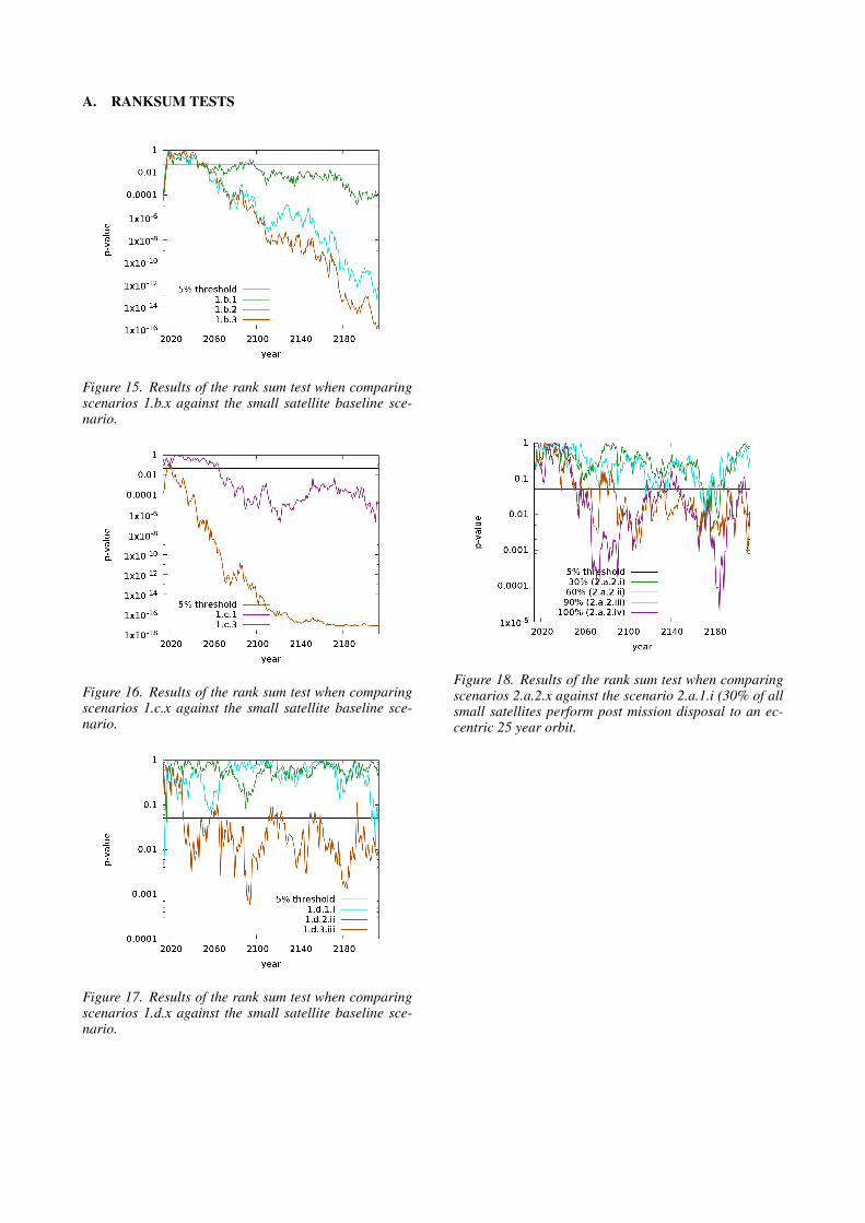
A. RANKSUM TESTS

Figure 15. Results of the rank sum test when comparingscenarios 1.b.x against the small satellite baseline sce-nario.

Figure 16. Results of the rank sum test when comparingscenarios 1.c.x against the small satellite baseline sce-nario.

Figure 17. Results of the rank sum test when comparingscenarios 1.d.x against the small satellite baseline sce-nario.

Figure 18. Results of the rank sum test when comparingscenarios 2.a.2.x against the scenario 2.a.1.i (30% of allsmall satellites perform post mission disposal to an ec-centric 25 year orbit.