The impact of technological and organizational changes on labor

flows. Evidence on French establishments.

Philippe Askenazy∗ Eva Moreno Galbis†

May 11, 2004

Abstract

This paper investigates the effect of organizational and technological changes on job sta-

bility of different occupations. We first develop a basic matching model with endogenous

job destruction. It predicts that new technologies should stimulate labor flows of low-skilled

workers, but innovative work organization has ambiguous consequences. Second, we exten-

sively exploit a unique French data set on a representative sample of French establishments.

Empirical results globally corroborate our theoretical predictions. The adoption of informa-

tion technologies increases flows of manual workers, employees and intermediary occupations.

In addition, tayloristic organization reduces flows of employees and manual workers, while

most of the new work practices raise employment variation of managers.

JEL classification: J23, J41, J63, L23, O33

Keywords: Job Flows; Information and Communication technologies; Organizational

Change

∗CNRS and CEPREMAP, 48 bd. Jourdan. 75014 Paris. philippe.askenazy@cepremap.ens.fr.†Universite Catholique de Louvain and IRES, Place Montesquieu, 3, B-1348 Louvain-la-Neuve (Belgique).

E-mail: moreno@ires.ucl.ac.be, moreno@delta.ens.fr

1

1 Introduction

The consequences of the information and communication technologies (ICT) revolution have

been largely analyzed by the economic literature. While authors like Berman, Bound, and

Griliches (1994), Fitz Roy and Funke (1995), Machin, Ryan, and Van Reenen (1998), Krusell

et al. (2000) and Moreno-Galbis (2002) claim that the capital-skill complementarity relation-

ship has led to a skill-biased technological change, other authors, like Caroli and Van Reenen

(2001) argue that it is the internal re-organization of firms following ICT adoption that has been

skill-biased. Nowadays, there is an increasing agreement about the complementary relationship

between ICT adoption, inside organizational changes of firms and skills (see Askenazy and Gi-

anella (2000), Bresnahan, Brynjolfsson, and Hitt (2002) Cappelli (1996), Caroli and Van Reenen

(2001) and Greenan (1996)). According to this argument, the introduction of ICT is necessarily

associated with changes in the organizational and skill infrastructure of the firms.

In spite of the numerous works about the effects of the ICT revolution, there is no much evidence

about its consequences on jobs quality. Our paper focuses on this issue, more particularly, we

explore the effects of new technologies and new organizational practices (introduced by firms

in order to efficiently exploit these ICT) on labor flows of different professional categories in

France.

There are many articles analyzing labor and jobs flows, such as Burgess and Nickell (1990), who

already in the beginning of the nineties developed a theoretical model distinguishing between the

determinants of quits and layoffs and estimated it working with UK data on the manufacturing

sector. Using Dutch data Hamermesh, Hassink, and Van-Ours (1996) describe the job flows

within a firm, the job flows to and from the firm, the net employment changes within a firm

and the patterns of hiring and firing. Burgess, Lane, and Stevens (2000), Neumark, Polsky, and

Hansen (1999) or Valletta (1999) analyze the evolution job stability (job security in the last

case) working with US data. Finally, using French data, Abowd and Kramarz (2003) address

the extent of entry and exit of workers associated with job creation and destruction, the role of

skill in simultaneous hiring and separation rates and the importance of short-term and long-term

contracts in the adjustment process. None of these papers analyzes the sources of labor and job

flows. The authors compute and describe flows without wondering about the effects that ICT

2

adoption, introduction of high performance workplace organizational (HPWO) practices (such

as delayering1, team work, decentralization of decision making within firms, quality control,

Total Quality Management) or other factors may have over these flows.

ICT1 investment

HPWO2 practices

in OECD countries

1980 1990 2000 Task Working Higher Reduction

rotation teams worker implication in hierarchy

Belgium .. .. 12 .. .. .. ..

France 6.1 8.5 13.1 6 30 44 21

Germany 7.7 13.9 19.2 7 20 19 30

Italy 8.0 14.2 16.7 13 28 24 10

Netherlands 11.2 15.5 20.9 9 9 46 47

Spain 5.6 11.9 10.1 14 34 33 ..

United Kingdom 5.6 13.8 22.0 13 33 48 45

United States 15.2 22.5 31.4 .. .. .. ..

1. Percentage of non residual gross fixed capital formation, total economy. ICT equipment is defined as computer and office

equipment and communication equipment; software includes both purchased and own account software.

2. Percentage of establishments stating in 1996 some of the HPWO practices adopted by their employers during the three

previous years (concerning Italy data refers to the three previous months).

.. Unavailable data.

Source concerning ICT: OECD estimates based on national accounts.

Source concerning HPWO: OECD Employment Outlook 1999, table 4.4, page 206.

Table 1: ICT investment and adopted HPWO practices in some OECD countries.

When comparing the scarce available data about the introduction of ICT and HPWO practices

with the also non abundant data concerning the workers’ feeling on job stability2, we observe that

in most European countries new technologies and innovative organizational practices adoption1Delegating responsibilities to lower hierarchical levels inside the firm by removing one or more managerial

levels.2It would be more interesting to compare the adoption of ICT and HPWO practices with the evolution of job

turnover, however the available data on this variable concerns, for most European countries, the average values

of job turnover between the mid-eighties and the beginning of the nineties (see OECD (1996) table 5.1 page 176),

therefore we cannot analyze its evolution.

3

Feeling1 of job instability Evolution2 of job instability

1996 1985-1995

Belgium 71.5 -6*

France 78.7 -14*

Germany 71.8 -18*

Italy 69.6 -5*

Netherlands 60.3 -12*

Spain 71.2 ..

United Kingdom 66.9 -22*

United States .. ..

1. Percentage of workers being in total disagreement with the statement my job is ensure.

2. Evolution in percentage points in the proportion of workers answering favorably to the question concerning the stability

of their job.

.. Unavailable data. * Significant evolution.

Source: OECD Employment Outlook 1997, table 5.2, page 148, and table 5.3, page 149.

Table 2: Job instability in OECD countries.

has been associated to an increased feeling of job instability by workers (see tables 1 and 2).

Using a unique French data set this paper tries to estimate the effects of ICT and HPWO

practices on the labor flows of different professional categories.

Related theoretical literature concerns Michelacci and Lopez-Salido (2004). On the empirical

side, Bauer and Bender (2002), working with a German employer-employee matched panel data

set, examine the impact of ICT and HPWO practices on gross job and worker flows. The authors

conclude that the organizational change is skill-biased since it leads to higher job destruction and

separation rates for low- and medium-skilled workers, while employment patterns of high-skilled

are not affected significantly. They also find that new technologies do not have significant effects

on gross job and workers flows. Neumark and Reed (2004), working with US data, estimate a

positive link between new economy jobs, defined either as employment in high-tech cities or as

industry employment growth, and contingent3 or alternative4 employment relationships. Jones,

Kato, and Weinberg (2003) implement a case study over ten US manufacturing establishments3A contingent worker is defined as an individual holding a job that is temporary by its nature.4Alternative employment arrangements are: independent contractors, on-call workers, temporary help agency

workers and workers provided by contract firms.

4

in order to determine how the quality of jobs is affected by the managerial decision on business

strategy. They conclude that in medium sized-establishment located in depressed areas and with

workers of low-educational level, the proper adoption of HPWO practices can yield favorable

worker outcomes: workers are more empowered, satisfied, committed, trusting, communicative

and hardworking. Moreover, on the basis of the European Survey on Working Conditions,

Bauer (2004) also finds that higher involvement in HPWO practices is associated with higher

job satisfaction. Finally, Givord and Maurin (2004), using the French Labor Force Survey,

develop an econometric analysis trying to identify the structural factors that have driven the

upturn in the risk of involuntary job loss experienced by French workers over the last 20 years.

They conclude that technological change seems to be at the origin of the increased job insecurity,

but its effect may be mitigated by institutional changes. Our paper tests this hypothesis (impact

of ICT) at the plant level.

This paper is divided in two interrelated parts. The first part develops a simple theoretical model

that provides a structure for implementing the empirical analysis of the second part. Since we

are concerned about the effects of new technologies and innovative organizational practices over

the labor flows, we try to embed these features in a basic theoretical setup. Mortensen and

Pissarides (1994) endogenous job destruction model provides an appropriate framework to do

so. More particularly, we consider a perfectly segmented labor market where we distinguish

between simple jobs, occupied by low-skilled workers, and complex jobs, occupied by high-

skilled workers. Each type of job is characterized by a constant productivity component which

is modified in case of biased technological or organizational changes.

In the second part of the paper we implement an empirical analysis. We use a database re-

sulting from merging two French surveys conducted in 1999 and covering more than twenty-five

hundred establishments: the REPONSE survey (RElations PrOfessionnelles et NegotiationS

d’Entreprise), which describes the use of new technologies and innovative organizational prac-

tices by the establishment, and the DMMO survey (Declaration Mensuelle de Mouvements de

main d’Oeuvre), describing the labor flows in the establishment by gender, age, professional cat-

egory, etc. We estimate the effects of ICT and HPWO practices on the labor flows of different

categories of workers. Results reveal that, in France, labor flows of blue collars are increased by

5

ICT adoption while the turnover of white collars are stimulated by some of the HPWO practices.

Our approach is focused on the total number of movements by professional categories while the

analysis developed in Bauer and Bender (2002) estimated job creation and destruction patterns

for different skill groups as well as worker replacement rates inside plants. Findings in both

studies can, thus, be considered as complementary.

The paper is organized as follows. Section 2 presents a basic theoretical model providing the

structure for our empirical analysis . The comparative static analysis reveals that the introduc-

tion of any technological or organizational change relatively favoring the productivity of white

collars stimulates labor flows of blue collars. In contrast any change favoring the relative pro-

ductivity of blue collar workers increases labor flows of white collars. Section 3 describes both,

the data surveys and the data itself. Section 4 develops the econometric analysis and results are

explained in Section 5. Section 6 concludes.

2 A simple model

2.1 Assumptions

We develop a basic model giving a theoretical foundation of the effects of ICT and HPWO

practices on job stability. This theoretical setup is inspired in a discrete version of Mortensen

and Pissarides (1994), developed in Cahuc and Postel-Vinay (2002) for the case of one firm

offering different types of contracts to homogenous workers. Here we assume two types of

competitive firms employing labor as a unique input:

• Firms producing a complex good only employ high-skilled workers since the production of

these goods involves complex task requiring a high-skill qualification.

• Firms producing simple goods only employ low-skilled workers since their production pro-

cess involves simpler tasks.

Therefore we have completely segmented labor markets, where high-skilled workers only occupy

complex jobs and low-skilled workers simple jobs (no job competition).

When the firm opens a vacancy, it can be filled and start producing or remain empty and

continue searching. Any job that is not producing or searching is destroyed (job destruction).

6

In contrast, a job is created when a firm with a vacant job and a worker meet and both decide

to start producing (it is mutually profitable to produce). The number of complex and simple

contacts per period (M ct and M s

t ) is respectively represented by the following linear homogeneous

matching functions:

M ct = M c(vc

t , uht ) and M s

t = M s(vst , u

lt) (1)

where vct and vs

t represent the number of complex and simple vacancies and uht and ul

t the

number of high- and low-skilled unemployed normalized by the fixed labor force size (which is

itself assumed equal to one).

We denote labor market tensions in the complex and simple segment by θct and θs

t , where:

θct ≡

vct

uht

and θst ≡

vst

ult

. (2)

The probabilities of filling a complex and a simple job vacancy are respectively decreasing in θct

and θst and they are defined as:

M ct

vct

= q(θct ) and

M st

vst

= q(θst ). (3)

With linear homogeneous matching functions, the probabilities of finding a complex or a simple

job can be respectively written as follows:

M ct

uht

= θctq(θ

ct ) and

M st

ult

= θst q(θ

st ). (4)

The complex job is associated to a fixed coefficients technology requiring one high-skilled worker

to produce ε+h1 units of output in period t. The simple job is associated to a fixed coefficients

technology requiring one low-skilled worker to produce ε + h2 units of output in period t. The

term ε is a random idiosyncratic productivity parameter which is the same whether we are

considering complex or simple jobs. All the values of ε are drawn from the distribution φ =

Φ′ over the interval [ε, ε], for both, complex and simple jobs. The process that changes this

idiosyncratic term is Poisson with arrival rate λ ε [0, 1]. Therefore, there exists a probability λ

that the job is hit by a shock such that a new value of ε has to be drawn from φ. The terms

h1 et h2 addition to one (h1 + h2 = 1) and they can be interpreted as the constant productivity

component specific to each production sector (complex sector or simple sector).

7

It is important to notice that all job contacts do not lead to a job creation, since the match may

not be productive enough. The initial productivity level ε + h1 (or ε + h2) is revealed to the

firm and the worker immediately after the match is formed. Because search and hiring activities

are costly, the productivity level may be too low to compensate either party for their efforts.

Therefore, there exists a productivity level, called reservation productivity and denoted εc for

the complex segment and εs for the simple one, below which it is not in the interest of the firm

and the worker to trade.

2.2 Concepts and notation

An open vacancy can remain empty and searching or be filled and start producing. The associ-

ated asset value to each of these situation is represented by Πvc(resp. Πvs

) when the complex

(resp. simple) vacancy is empty and by Πc(ε) (resp. Πs(ε)) when the complex (resp. simple)

vacancy is filled. In the same way, the value to the worker in a complex (resp. simple) job is

denoted as V c(ε) (resp. V s(ε)). Finally, the average expected return on the high-skilled (resp.

low-skilled) worker’s human capital when looking for a job is represented by V uh(V ul

). Since

search and hiring activities are costly, when a match is formed a joint surplus is generated:

Sc(ε) = Πc(ε)−Πvc+ V c(ε)− V uh

Joint surplus in a complex job.

Ss(ε) = Πs(ε)−Πvs+ V s(ε)− V ul

Joint surplus in a simple job.

At the beginning of every period the firm and the employee renegotiate wages through a Nash

bargaining process, that splits the joint surplus into fixed proportions at all times. Denoting as

η ε [0, 1] the bargaining power5 of workers (whether they are in complex or simple positions),

we have that:

Πc(ε)−Πvc= (1− η) Sc(ε) or V c(ε)− V uh

= η Sc(ε) , (5)

Πs(ε)−Πvs= (1− η) Ss(ε) or V s(ε)− V ul

= η Ss(ε) . (6)

When a firm producing a complex good opens a vacancy it has to support a cost ac per unit

of time. When a firm producing a simple good opens a vacancy it has to support a cost as per

unit of time. There is a probability 1−q(θc) and 1−q(θs) that the complex and simple vacancy,5For proofs we will exclude the extreme cases η = 0 and η = 1.

8

respectively, remain empty next period. On the opposite, there is a probability q(θc) and q(θs)

that the complex and the simple vacancies get filled. The asset value associated to a searching

vacancy is then:

Πvc= −ac + β (1− q(θc)) Πvc

+ β q(θc)∫ ε

εMax[Πc(x), Πvc

] dΦ(x) , (7)

Πvs= −as + β (1− q(θs)) Πvs

+ β q(θs)∫ ε

εMax[Πs(x), Πvs

] dΦ(x) . (8)

where β is the discount factor.

When the vacancy is filled and actively producing, we know that there is a probability λ that

the job is hit by a shock, so that a new value of ε is drawn from the distribution φ. The asset

values associated to the complex and simple jobs are respectively:

Πc(ε) = ε + h1 − wc + β (1− λ) Max[Πc(ε),Πvc] + β λ

∫ ε

εMax[Πc(x),Πvc

] dΦ(x) ,(9)

Πs(ε) = ε + h2 − ws + β (1− λ) Max[Πs(ε), Πvs] + β λ

∫ ε

εMax[Πs(x), Πvs

] dΦ(x) ,(10)

where wc and ws represent, respectively, the wages paid to a high- and a low-skilled workers.

Independently of her skills, an unemployed worker receives a flow of earnings wu including

unemployment benefits, leisure, etc. The high-skilled job seeker comes in contact with a complex

vacant slot at rate θcq(θc) while the low-skilled comes in contact with a simple vacancy at rate

θsq(θs). The value to the workers of unemployment is given by:

V uh= wu + β (1− θcq(θc)) V uh

+ βθcq(θc)∫ ε

εMax[V c(x), V uh

] dΦ(x) (11)

V ul= wu + β (1− θsq(θs)) V ul

+ βθsq(θs)∫ ε

εMax[V s(x), V ul

] dΦ(x) . (12)

As just mentioned, a complex job with productivity ε + h1 pays a wage wc to the worker, while

a simple job with productivity ε + h2 pays ws. Both types of jobs are hit by a shock with

probability λ. The present value of a complex and simple job to the worker solve:

V c(ε) = wc + β (1− λ) Max[V c(ε), V uh] + β λ

∫ ε

εMax[V c(x), V uh

] dΦ(x) , (13)

V s(ε) = ws + β (1− λ) Max[V s(ε), V ul] + β λ

∫ ε

εMax[V s(x), V ul

] dΦ(x) . (14)

9

2.3 Job Creation and Job Destruction

We develop in detail the calculus of the steady state in appendix 1. This section presents the

equilibrium job creation and job destruction rules obtained for each labor market segment. Job

creation rules of the complex and simple segments are defined as:

ac

β(1− η) q(θc)=

11− β(1− λ)

∫ ε

εc

(1− Φ(x)) dx , (15)

as

β(1− η) q(θs)=

11− β(1− λ)

∫ ε

εs

(1− Φ(x)) dx , (16)

As shown in appendix 1, both equations determine a negative relationship between market

tightness and ε, meaning that the job creation curves are negatively sloped in the space (θi, ε)

for i = c, s.

Complex and simple job destruction rules are given by:

η ac θc

1− η= εc + h1 − wu +

β λ

1− β(1− λ)

∫ ε

εc

(1− Φ(x)) dx , (17)

η as θs

1− η= εs + h2 − wu +

β λ

1− β(1− λ)

∫ ε

εs

(1− Φ(x)) dx . (18)

It is proved in the appendix that both curves are positively sloped in the space (θc, ε) and (θs, ε),

respectively.

2.4 Comparative Static Analysis

We analyze now the variations in job creation and destruction predicted by the model when

some exogenous biased shocks modify the specific productivity component of each sector. The

theoretical results described in this section permit to better understand the empirical findings

presented afterwards.

Notice first, that depending on the values of h1, h2, θc, θs, ac and as, we might have an initial

situation where the reservation productivity levels are such that: εc > εs or εc < εs or εc = εs. In

any case, since the objective of the static comparative analysis we implement is to determine the

evolution (increase or decrease) in the turnover of complex and simple jobs, the initial situation

does not matter for the analysis . We focus on the effects of ICT and HPWO practices in each

market segment separately.

10

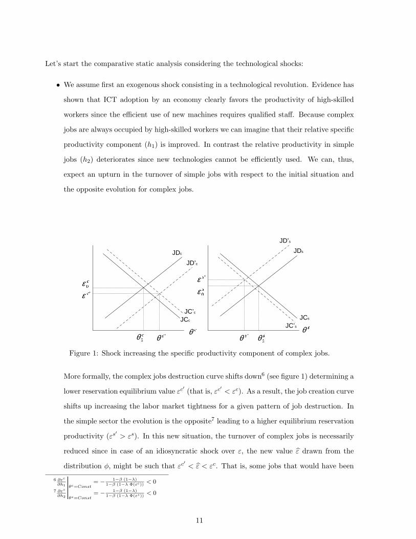
Let’s start the comparative static analysis considering the technological shocks:

• We assume first an exogenous shock consisting in a technological revolution. Evidence has

shown that ICT adoption by an economy clearly favors the productivity of high-skilled

workers since the efficient use of new machines requires qualified staff. Because complex

jobs are always occupied by high-skilled workers we can imagine that their relative specific

productivity component (h1) is improved. In contrast the relative productivity in simple

jobs (h2) deteriorates since new technologies cannot be efficiently used. We can, thus,

expect an upturn in the turnover of simple jobs with respect to the initial situation and

the opposite evolution for complex jobs.

�

θ�

θ�

��

θ�

��

θ

�

ε

�

�ε�

�ε

�

ε

JCc

JDc

JD’c

JCs

JD’s

JDs

JC’s

JC’c

Figure 1: Shock increasing the specific productivity component of complex jobs.

More formally, the complex jobs destruction curve shifts down6 (see figure 1) determining a

lower reservation equilibrium value εc′ (that is, εc′ < εc). As a result, the job creation curve

shifts up increasing the labor market tightness for a given pattern of job destruction. In

the simple sector the evolution is the opposite7 leading to a higher equilibrium reservation

productivity (εs′ > εs). In this new situation, the turnover of complex jobs is necessarily

reduced since in case of an idiosyncratic shock over ε, the new value ε drawn from the

distribution φ, might be such that εc′ < ε < εc. That is, some jobs that would have been

6 ∂εc

∂h1

���θc=Const

= − 1−β (1−λ)1−β (1−λ Φ(εc))

< 0

7 ∂εs

∂h2

���θs=Const

= − 1−β (1−λ)1−β (1−λ Φ(εs))

< 0

11

destroyed in the initial situation, are not destroyed now that the specific productivity

component of complex jobs has increased and the reservation productivity decreased. On

the contrary, in the the simple segment job turnover is stimulated since the reduction of the

specific productivity component determines a higher equilibrium reservation productivity,

(εs′ > ε > εs).

• We consider now a shock of a completely different nature. We assume that chain production

systems (tayloristic systems) are introduced in both sectors of the economy. Such a change

is likely to improve the relative marginal productivity of simple jobs (h2) reducing their

turnover. Because we are considering biased shocks (h1 + h2 = 1) an improvement in the

marginal productivity of simple jobs implies a deterioration in that of complex jobs (fall in

h1). In graphical terms (see figure 2), the job destruction curve of the simple segment shifts

right, determining a lower equilibrium reservation productivity in this market (εs′ < εs),

while in the complex segment the job destruction curve moves upward leading to εc′ > εc.

In this new situation, we require a stronger idiosyncratic shock over ε, with respect to the

initial situation, to have simple jobs destroyed. On the contrary the idiosyncratic shock

required to destroy complex jobs is now weaker.

In sum, technological shocks stimulate turnover in the labor market segment (complex or simple)

whose specific productivity component is negatively affected by the shock, while turnover falls

in the segment with an improved relative productivity. The static comparative analysis con-

cerning the introduction of HPWO practices follows this same principle. We briefly comment

the consequences on labor turnover of some particular HPWO practices:

• One of the main HPWO practices implemented by firms consists in introducing au-

tonomous teams of production and multidisciplinary or project working groups. As Jones,

Kato, and Weinberg (2003) show, these new organizational practices permit low-skilled

workers to get more empowered with the firm, to be more satisfied, more committed and

trusting in the managerial structure as well as more hardworking. Therefore, we can ex-

pect that such organizational practices improve the specific productivity component of

simple jobs (h2) while deteriorating that of complex jobs (h1). Turnover is, thus, reduced

in the simple segment and augmented in the complex segment (figure 2) .

12

• Another commonly used HPWO practice consists in implementing total quality control

procedures. Evidently this control can only be implemented by qualified workers, which

implies that the relative productivity of high-skilled workers is improved with respect to

that of low-skilled (figure 1).

• The rotation of workers among different tasks or the just in time production practices inside

firms are more likely to affect production workers (simple sector) rather than managers

(complex sector). The main objective of such practices is not simply to form workers

with more flexible abilities which permits firms to easily adapt to market demand changes,

but also to avoid workers loosing motivation due to repetitive tasks. The adoption of the

rotation or the just in time production systems is then likely to stimulate the relative

specific productivity component of simple jobs, reducing in this way their turnover. On

the contrary, the turnover of high-skilled workers is stimulated (figure 2).

�

θ�

θ�

��

θ�

��

θ

�

ε�

�ε

�

�ε�

ε

JCc

JDc

JD’c

JCs

JD’s

JDs

JC’s

JC’c

Figure 2: Shock increasing the specific productivity component of simple jobs.

• The introduction of the HPWO practice consisting in delayering (delegating responsibili-

ties to lower hierarchical levels inside the firm by removing one or more managerial levels),

stimulates the relative productivity specific component of production workers (simple jobs)

deteriorating that of managers in the firm (complex jobs). This measure is then likely to

raise the turnover of complex jobs and decrease that of simple jobs (figure 2). Indeed

in Caroli and Van Reenen (2001) it is shown that, in the French case, the reduction in

13

the number of hierarchical levels (delayering) has mainly favored skilled manual workers,

whose wage bill share has been increased.

3 The data

The database used results from merging two French surveys conducted in 1999 and refereing to

1998: the REPONSE survey (RElations PrOfessionnelles et NegotiationS d’Entreprise) and the

DMMO survey (Declaration Mensuelle de Mouvements de main d’Oeuvre).

In REPONSE more than twenty-five hundred establishments were surveyed with senior man-

agers being asked about the economic situation of the establishment, its internal organization,

technological changes, the wage negotiation with unions and conflicts with workers. Only estab-

lishments with 20 or more employees were sampled and no public sector employees were included

(except workers in state-owned industries). Concerning ICT and HPWO practices, managers

were asked either about their presence in the establishment (1993 and 1998 waves) either about

the proportion of workers benefitting from the corresponding technology or workplace practice

(1998 wave). The REPONSE survey, which is also used in Caroli and Van Reenen (2001),

contains, thus, very detailed information on the technological and organizational practices of a

representative sample of French establishments.

In the DMMO survey, each establishment with at least 50 employees makes a monthly declaration

of the beginning-of-the-month employment, end-of-the-month employment and the total entries

and exists within the month. Furthermore, the respondent establishment reports the nature of

the employment transaction (type of contract of the new entries and reasons for the exit), as

well as the skill level, age and seniority of the employee involved in this transaction.

In the present paper we consider the effect that different technological and organizational vari-

ables have on the labor flows of five professional categories (all workers, managers, intermediary

professions, employees and manual workers) as well as on women and men. We work with a

cross section referred to 1998. Since the REPONSE survey and the DMMO survey were both

conducted also in 1993, there does exist a small panel referring to 1993 and 1998. Unfortunately

14

its reduced size and the highly probably presence of a bias leads to meaningless estimations. We

explain below the variables used in the econometric analysis.

3.1 Labor flows

The variables capturing the workers flows of different professional categories are defined as

follows:

• TOTAL=(Number of movements of all the workers in the establishment)/Total number

of workers in the establishment.

• MANAGERS=(Number of movements of managers in the establishment)/Total number

of managers in the establishment.

• INT. PROFES.=(Number of movements of intermediary professionals in the establish-

ment)/Total number of intermediary professionals in the establishment.

• EMPLOYEES=(Number of movements of employees in the establishment)/Total number

of employees in the establishment.

• WORKERS=(Number of movements of manual workers in the establishment)/Total num-

ber of manual workers in the establishment.

• WOMEN=(Number of movements of women in the establishment)/Total number of women

in the establishment.

• MEN=(Number of movements of men in the establishment)/Total number of men in the

establishment.

The number of movements is defined as the sum of entries and exits.

3.2 Technological variables

New technologies, specially ICT, are widely spread on French establishments, therefore we con-

sider two technological variables:

• COMPUTER: It is a dummy variable taking the value 1 if 50% or more workers use a

computer.

15

• NET: It is a dummy variable taking the value 1 if between 20 and 50% of the workers use

the net system.

In addition, automated production is captured by the variable:

• CHAIN: It is a dummy variable taking the value 1 when the establishment still uses

tayloristic production systems (robots, computer assisted systems, etc.).

3.3 Organizational variables

To measure the effects of HPWO practices we consider six different variables:

• AUTONOMOUS: It is a dummy variable taking the value 1 if between 20 and 50% of the

workers participates in autonomous teams of production.

• PROJECT: It is a dummy variable taking the value 1 if between 20 and 50% of the workers

participates in multidisciplinary working groups or project groups.

• ROTATION: It is a dummy variable taking the value 1 when a majority of workers rotates

among tasks inside the firm.

• QUALITY: It is a dummy variable taking the value 1 when the establishment develops a

total quality control procedure.

• HIERARCHY: It is a dummy variable taking the value 1 when the establishment has

reduced the number of hierarchical levels.

• JUST TIME: It is a dummy variable taking the value 1 when the establishment practices

just in time production methods.

3.4 Other variables

In the regressions we control for the size of the establishment, the economic sector, the relative

importance of employees, technicians, short term contracts and women in the establishment

and we also consider whether the establishment has already implemented the reduction in the

number of working hours (35 hours per week). We define these variables as:

16

• Size: Dummy variable taking the value 1 if the number of workers in the firm is between

50 and 500.

• Hours: Dummy variable taking the value 1 if the firm has already implemented the reduc-

tion in the number of working hours.

• % Employees and % Technicians are the percentage of employees and technicians in the

establishment.

• % Women is the percentage of women in the establishment.

• % Contract is the percentage of fixed duration contract in the establishment.

• Energy, Building, Finance, Services firms, Services individuals, Education and Adminis-

tration are sectorial variables. They represent respectively the following sectors: energy

sector (Energy); building sector (Building); financial activity sector (Finance); services to

firms (Services firms); services to individuals (Services individuals); education, health and

social action (Education); and administration (Administration).

3.5 Descriptive statistics

Appendix 3 summarizes the means and standard deviation of all variables used in our model.

Remark that the category of workers having the relatively most important turnover are the

employees, followed by the managers, the intermediate professionals and the manual workers.

Even if the manual workers are those with the smallest labor flows, they have also the smallest

standard deviation, which contrast with the high standard deviation of mangers or employees.

Most of these labor flows correspond to women.

Notice also, the high presence of chain production systems and the importance of organizational

practices such as the reduction of hierarchical levels, just in time production systems and the

implementation of quality control procedures.

Appendix 4 presents the correlation matrix between labor flows, technological variables and

organizational variables. In the upward part of the table we present the pairwise correlations

between the labor flows and the technological and organizational variables of the model. In the

17

downward part of the table we present the pairwise correlations between the technological and

the organizational variables.

From the first part of the table, we remark the positive correlation between the labor flows

of manual workers with respect to COMPUTER and NET. This contrast with the systemat-

ically negative correlation observed for labor flows and CHAIN. Organizational practices such

as rotation of workers among different tasks, total quality control procedures or the reduction

of hierarchical levels are negatively correlated with the turnover of intermediate professionals,

employees and manual workers. In contrast, AUTONOMOUS and PROJECT are positively

related to the managers’ turnover.

From the second part of the table we remark that the use of new technologies and the introduction

of new organizational practices are most of the times positively correlated (complementary

relationship). However, the rotation of workers among task or the just in time production

systems are negatively correlated with COMPUTER and NET. A negative correlation between

the autonomous teams of production and COMPUTER is also observed.

4 Econometric modelling

According to our structural model, any technological or organizational change improving (dete-

riorating) the relative productivity of a particular professional category should reduce (increase)

its turnover. More particularly we have seen that ICT adoption stimulates the turnover of pro-

duction workers (simple jobs) while most HPWO practices increase the turnover of managers

(complex jobs). We proceed now to estimated the following econometric model:

Yiet = α1 Iiet + α2 Oiet + α3 Xiet + υiet (19)

where the dependent variables are the labor flows of all workers, of managers, intermediary

professions, employees, manual workers, women workers and men workers. The vector Iiet con-

tains all variables measuring the presence of information and communication technologies in

the establishment. These variables are COMPUTER, NET and CHAIN. We expect α1 > 0 for

intermediary professions, employees and manual workers, and α1 < 0 for managers. The vector

18

Oiet consists on all variables describing the introduction of HPWO practices by the establish-

ment. It contains: AUTONOMOUS, PROJECT, ROTATION, QUALITY, HIERARCHY and

JUST TIME. In this case, we expect α2 > 0 for managers and α2 < 0 for the rest of workers

categories. Finally Xit is the vector of controls, where we introduce other variables that could

affect the labor flows. More particularly, we control for the size of the firm, the number of hours

worked in the establishment, the sector of activity, the percentage of employees, technicians and

women in the establishment, as well as the percentage of workers with fixed duration contract.

Because the percentage of workers with short term contract may be endogenous, we estimate

the model twice, once controlling for this variable and the other without controlling for it.

Another econometric problem that we must solve concerns the selection bias that is likely to

be present when considering the labor flows of manual workers. Indeed less than half of the

establishments have manual workers employed. Furthermore, since many of these establishments

belong to the service sector, it seems logical that those employing manual workers will present

particular characteristics. Therefore the risk of a selection bias arises and applying the Heckman

selection model for the labor flows of manual workers seems convenient. According to this

method, in the relationship:

WORKERSet = α1 Iet + α2 Oet + α3 Xet + υet (20)

the dependent variable is not always observed. Its observability will depend in a certain number

of characteristics. Therefore, the Heckman selection model estimates first:

y∗t = β Zt + ut , (21)

where y∗t is the probability to observe a manual worker labor flow and Zt a vector containing

technological and organizational variables, as well as variables concerning the economic situation

of the firm, its size, its labor composition, its economic sector, its investment on training workers

and its internal conflicts. Notice that,

WORKERSt = 1 if y∗t > 0 (22)

WORKERSt = 0 otherwise . (23)

On the basis of this result the relationship (20) is re-estimated without selection bias this time.

Indeed when corr(υt, ut) = ρ > 0, the Heckman selection model provides consistent, asymp-

19

totically efficient estimates for all parameters. Therefore we directly implement this procedure

when dealing with manual workers turnover.

5 Results

5.1 Effect of ICT and HPWO practices

Final estimates from the regressions are reported in tables 3 and 4 (see table 7 in appendix 2 for

reference on the set variables initially used, before eliminating the least significant variables). In

the former table the percentage of fixed duration contracts in the establishment is introduced

as a control variable, while in table 4 we do not control for this variable. Results are essentially

the same in both cases, suggesting that there is not endogeneity problem with the variable %

Contract.

This paper tries to shed some light regarding the deterioration or the improvement in the quality

of jobs due to the introduction of ICT and/or HPWO practices. Empirical results obtained in

this section reveal that the effects of these variables differ, and are even contradictory, depending

on the professional category under analysis.

Consider first the labor flows of all workers (i.e: all professional categories confounded). Results

suggest that the organizational practice consisting in the rotation of workers among different

tasks inside the establishment stimulates workers’ flows while the more traditional chain pro-

duction systems (tayloristic system) reduce these flows. The analysis becomes more interesting

when considering separately each professional category:

• The managers’ turnover is stimulated by the just in time production systems and the or-

ganizational practices targeting to improve the workers and employees’ empowerment and

commitment to the firm, such as the autonomous teams of production or multidisciplinary

groups. On the contrary, the organizational practice consisting in implementing total

quality control procedures reduces the labor flows of managers, as this practice requires

qualified staff to be developed.

• We look now results concerning intermediate professionals, employees and manual workers.

Starting with the intermediate professionals we realize that the massive use of computers

20

Table 3: Determinants of labor flows for different categories of workers controlling for short term

contracts.

Dependent variable: labor flows for

TOTAL MANAGERS INT. PROFES. EMPLOYEES WORKERS WOMEN MEN

COMPUTER 0.102 -1.386 0.554 0.551 0.070 0.033 0.159

(0.093) (1.303) (0.195)*** (0.292)* (0.189) (0.289) (0.160)

NET -0.054 -0.412 0.144 -0.070 0.286 -0.228 -0.191

(0.091) (1.247) (0.183) (0.283) (0.175)* (0.279) (0.154)

CHAIN -0.120 0.135 0.058 -0.418 -0.235 -0.364 -0.196

(0.051)** (0.698) (0.102) (0.156)*** (0.094)** (0.154)** (0.085)**

AUTONOMOUS 0.006 2.175 0.038 -0.161 -0.061 -0.242 0.126

(0.089) (1.220)* (0.177) (0.278) (0.158) (0.273) (0.150)

PROJECT -0.022 2.451 -0.127 0.044 -0.197 0.255 -0.117

(0.087) (1.190)** (0.175) (0.270) (0.172) (0.264) (0.146)

ROTATION 0.116 -1.217 0.082 0.226 -0.113 0.176 0.101

(0.081) (1.123) (0.163) (0.253) (0.147) (0.247) (0.137)

QUALITY -0.023 -2.498 0.197 -0.011 -0.090 0.036 0.158

(0.078) (1.092)** (0.161) (0.244) (0.159) (0.240) (0.133)

HIERARCHY -0.045 0.774 -0.140 -0.345 0.039 -0.157 -0.076

(0.051) (0.708) (0.104) (0.160)** (0.096) (0.156) (0.086)

JUST TIME 0.068 1.118 -0.044 -0.043 0.091 0.164 0.085

(0.043) (0.606)* (0.088) (0.136) (0.079) (0.134) (0.074)

Size -0.042 -0.220 0.149 -0.452 0.129 -0.410 -0.120

(0.086) (1.186) (0.173) (0.266)* (0.164) (0.263) (0.145)

Hours 0.016 4.024 0.274 -0.306 -0.023 -0.109 -0.056

(0.108) (1.479)*** (0.215) (0.337) (0.192) (0.330) (0.182)

% Employees 0.623 2.954 0.523 -2.756 3.254 1.510 0.520

(0.150)*** (2.084) (0.309)* (0.459)*** (0.451)*** (0.454)*** (0.250)**

% Technicians -0.196 -0.472 -2.781 -1.195 0.820 -1.260 -0.075

(0.246) (3.464) (0.525)*** (0.808) (0.578) (0.768)* (0.423)

% Women 0.333 0.646 0.416 1.837 0.603 -3.976 1.948

(0.156)** (2.162) (0.318) (0.481)*** (0.306)** (0.474)*** (0.261)***

% Contract 0.434 -4.730 0.570 2.351 1.185 0.616 -0.047

(0.340) (4.607) (0.670) (1.025)** (0.689)* (1.029) (0.566)

Sectors (16) YES YES YES YES YES YES YES

Constant 0.411 -1.153 0.257 1.486 -0.035 2.300 0.047

(0.127)*** (1.780) (0.264) (0.396)*** (0.247) (0.390)*** (0.215)

Adj. R2 0.119 0.032 0.122 0.065 0.073 0.105

Observations 1645 1689 1575 1631 1140 1719 1722

*Significant at 10%.**Significant at 5%.***Significant at 1%.

21

by the establishment (when more than 50% of the staff uses them) is associated to a

higher flows of this category of workers. In contrast, the HPWO practices seem to have

no effect on this turnover. According to our model, these results indicate that, while the

ICT deteriorate the intermediate professionals’ relative productivity, the HPWO practices

must not have so much effect on it.

The massive use of computers in the establishment also increases job instability of employ-

ees. In contrast, the use of the tayloristic production systems as well as the organizational

practices consisting in removing managerial levels so as to delegate responsibilities to lower

hierarchical levels improve the relative productivity, motivation, commitment and empow-

erment of this worker category reducing its turnover.

The labor flows of manual workers are increased by the use of ICT which negatively affect

their relative marginal productivity. On the opposite, chain production systems permit

manual workers to improve their relative productivity, reducing in this way their turnover.

HPWO practices have no effect at all in manual workers’ job stability.

In sum, the use of ICT is clearly associated to higher labor flows of intermediate profession-

als, employees and manual workers. On the contrary, because chain production systems

improve the blue collar workers’ relative productivity, they also reduce the turnover of these

categories of workers. The progressive disappearance of the tayloristic systems would ex-

plain then the upturn in blue collars’ labor flows. The HPWO practices do not seem be

a key determinant on the labor flows of intermediate professionals and manual workers.

In contrast employees have clearly benefited from the organizational practice consisting in

delaying responsibilities to lower hierarchical levels.

• Equation (19) is also estimated for the women and men workers. Evidently, in this case all

workers categories are confounded, that is, inside women workers there will be managers

as well as manual workers and the same applies for men. Similarly to results concerning all

workers flows (TOTAL), we conclude that the introduction of chain production systems is

associated to lower labor flows of men and women.

22

Table 4: Determinants of labor flows for different categories of workers without controlling for

short term contracts.

Dependent variable: labor flows for

TOTAL MANAGERS INT. PROFES. EMPLOYEES WORKERS WOMEN MEN

COMPUTER 0.104 -1.287 0.559 0.537 0.099 0.038 0.168

(0.093) (1.291) (0.193)*** (0.290)* (0.187) (0.287) (0.158)

NET -0.056 -0.360 0.143 -0.090 0.289 -0.224 -0.189

(0.090) (1.235) (0.182) (0.281) (0.173)* (0.276) (0.152)

CHAIN -0.120 0.116 0.051 -0.423 -0.229 -0.363 -0.192

(0.050)** (0.688) (0.101) (0.155)*** (0.093)** (0.153)** (0.084)**

AUTONOMOUS 0.001 2.156 0.044 -0.135 -0.061 -0.256 0.124

(0.088) (1.207)* (0.176) (0.276) (0.157) (0.270) (0.148)

PROJECT -0.023 2.364 -0.117 0.091 -0.194 0.247 -0.121

(0.086) (1.177)** (0.173) (0.268) (0.171) (0.262) (0.144)

ROTATION 0.118 -1.116 0.086 0.213 -0.110 0.184 0.113

(0.080)* (1.110) (0.162) (0.251) (0.146) (0.245) (0.135)

QUALITY -0.107 -2.422 0.190 -0.015 -0.074 0.026 0.158

(0.077) (1.075)** (0.159) (0.241) (0.157) (0.238) (0.131)

HIERARCHY -0.046 0.786 -0.148 -0.360 0.033 -0.144 -0.077

(0.050) (0.699) (0.103) (0.158)** (0.095) (0.155) (0.085)

JUST TIME 0.064 1.065 -0.040 -0.052 0.083 0.164 0.081

(0.042) (0.598)* (0.087) (0.135) (0.785) (0.132) (0.073)

Size -0.042 -0.206 0.141 -0.489 0.140 -0.425 -0.124

(0.085) (1.174) (0.171) (0.264)* (0.163) (0.260)* (0.144)

Hours 0.007 3.851 0.276 -0.311 -0.004 -0.101 -0.064

(0.106) (1.457)*** (0.211) (0.333) (0.190) (0.325) (0.179)

% Employees 0.621 2.896 0.509 -2.785 3.078 1.530 0.515

(0.148)*** (2.054) (0.305)* (0.454)*** (0.441)*** (0.448)*** (0.247)**

% Technicians -0.194 0.511 -2.806 -1.300 0.647 -1.266 -0.077

(0.243) (3.417) (0.518)*** (0.800) (0.570) (0.760)* (0.418)

% Women 0.353 0.580 0.421 1.986 0.614 -3.938 1.942***

(0.153)** (2.122) (0.313) (0.474)*** (0.300)** (0.465)*** (0.256)

% Contract NO NO NO NO NO NO NO

Sectors (16) YES YES YES YES YES YES YES

Constant 0.431 -1.427 0.303 1.625 0.037 2.310 -0.051

(0.124)*** (1.735) (0.258) (0.387)*** (0.242) (0.381)*** (0.209)

Adj. R2 0.119 0.031 0.120 0.061 0.074 0.104

Observations 1669 1714 1595 1656 1156 1744 1747

*Significant at 10%.**Significant at 5%.***Significant at 1%.

23

To summarize, empirical estimates suggest that, since ICT are skill-requiring, its adoption re-

sults in higher turnover of intermediate professionals, employees and manual workers, who do

not have these skills. At the same time, the turnover of these categories of workers falls when

the establishment adopts tayloristic production systems. Because most HPWO practices try to

stimulate motivation, participation and productivity of blue collar workers (production workers),

its adoption is associated to higher labor flows of managers, whose relative productivity is nega-

tively affected by these organizational practices. To conclude notice that, since ICT adoption is

generally accompanied by changes in the internal organization of firms (HPWO practices), we

can suggest that the labor flows of all workers categories must have been stimulated over the

last years, either through the ICT for the blue collars, either by the HPWO practices for the

white collars. Moreover, the reduction in the use of chain production systems has reinforced job

instability of all workers categories.

5.2 Solving the Endogeneity Bias

The high degree of intercorrelation among the explicative variables (see table 9) indicates that

the empirical model estimating the impact of the ICT and HPWO practices on the labor flows

may yield biased coefficients. To solve this endogeneity problem a traditional approach used in

the literature (e.g., Ichniowski, Shaw, and Prennushi (1997)) when only cross-sectional data is

available, consists in defining sets of highly correlated practices. We consider in this paper two

types of clusters differing in their economic interpretation:

• We analyze first the impact of what we will call “incremental organization” or “additive

clusters”. These sets of practices capture a kind of continuity in the technological and

organizational changes.

• Second, we consider the effect of clusters including complementary technological and or-

ganizational practices (“multiplicative clusters”). There is an increasing literature (e.g.,

Ichniowski, Shaw, and Prennushi (1997) or Askenazy and Gianella (2000)) claiming that

firms realize the largest gains in productivity by adopting clusters of complementary prac-

tices. It seems, thus, relevant to analyze the effect that these sets of interactive practices

have on the labor flows.

24

5.2.1 The incremental organization

The incremental organization can be economically interpreted as measuring a continuity in

the process of introduction of technological and organizational changes. We define five sets of

variables capturing practices having a similar objective and being highly intercorrelated:

1. TECHNOLOGY: Cluster including the technological variables COMPUTER and NET.

The presence of one of these practices is sufficient to guarantee the non nullity of TECH-

NOLOGY.

2. CHAIN: Dummy variable taking the value 1 when the establishment still uses systems of

tayloristic production systems (robots, computer assisted systems, etc.).

3. TEAMWORK: Set of organizational variables including all practices tending towards

the delegation of responsibilities and the promotion of working teams. The positivity

of TEAMWORK is guaranteed by the presence of any of the following practices: AU-

TONOMOUS, PROJECT or HIERARCHY.

4. FLEXIBILITY: Cluster covering all organizational practices stimulating a flexible job as-

signment (ROTATION and JUST TIME).

5. QUALITY: Dummy variable taking the value 1 when the establishment develops a total

quality control procedure.

Results in table 5 can be summarized as follows:

• The upturn in job instability of all workers (TOTAL) seems to be explained, rather than

by the simple introduction of new technologies, by the combination of the progressive

reduction in the use of tayloristic production system and progressive increase in the use

of flexible job assignment practices.

• The workplace organizational practices favoring the delegation of responsibilities to lower

hierarchical levels as well as the presence of working teams (TEAMWORK) are at the

origin of the increased turnover observed for the managers. In contrast, quality control

procedures continue to have an stabilization effect on their turnover.

25

Table 5: Effect of incremental organization over the labor flows.

Dependent variable: labor flows for

TOTAL MANAGERS INT. PROFES. EMPLOYEES WORKERS WOMEN MEN

TECHNOLOGY 0.022 -0.767 0.330 0.248 0.179 -0.069 -0.030

(0.050) (0.693) (0.102)*** (0.156) (0.106)* (0.154) (0.085)

CHAIN -0.120 -0.113 0.058 -0.418 -0.236 -0.367 -0.194

(0.051)** (0.699) (0.102) (0.157)*** (0.094)*** (0.155)** (0.085)**

TEAMWORK -0.030 1.497 -0.100 -0.217 -0.036 -0.076 -0.044

(0.036) (0.495)*** (0.072) (0.111)** (0.067) (0.109) (0.060)

FLEXIBILITY 0.078 0.542 -0.016 0.016 0.040 0.161 0.087

(0.037)** (0.507) (0.073) (0.115) (0.066) (0.112) (0.062)

QUALITY -0.112 -2.434 0.187 -0.024 -0.088 0.037 0.152

(0.078) (1.091)** (0.161) (0.244) (0.160) (0.241) (0.133)

Size -0.040 -0.246 0.148 -0.449 0.131 -0.410 -0.121

(0.086) (1.187) (0.173) (0.266)* (0.164) (0.263) (0.145)

Hours 0.011 3.803 0.263 -0.336 0.000 -0.125 -0.068

(0.107) (1.471)*** (0.213) (0.336) (0.191) (0.328) (0.181)

% Employees 0.630 2.952 0.537 -2.719 3.243 1.542 0.537

(0.149)*** (2.075) (0.308)* (0.457)** (0.449)*** (0.452)*** (0.250)**

% Technicians -0.179 0.346 -2.713 -1.085 0.718 -1.144 -0.063

(0.245) (3.445) (0.520)*** (0.805) (0.575) (0.765) (0.421)

% Women 0.338 0.531 0.427 1.863 0.591 -3.967 1.958

(0.156)** (2.161) (0.318) (0.481)*** (0.306)** (0.473)*** (0.261)***

% Contract 0.436 -4.530 0.583 2.361 1.179 0.632 -0.050

(0.339) (4.608) (0.670) (1.025)** (0.690)* (1.028) (0.566)

Sectors (16) YES YES YES YES YES YES YES

Constant 0.403 -1.569 0.240 1.394 0.034 2.220 -0.053

(0.125)*** (1.752) (0.259) (0.389)*** (0.242) (0.384)*** (0.211)

Adj. R2 0.120 0.032 0.123 0.064 0.074 0.105

Observations 1645 1689 1575 1631 1140 1719 1722

*Significant at 10%.**Significant at 5%.***Significant at 1%.

26

• The only professional category whose turnover seems clearly to have been stimulated by

the ICT adoption is the intermediate professions.

• Regarding employees and manual workers, results in table 5 point to the progressive re-

duction in the tayloristic production systems as the main responsible of the increased job

instability of these professional categories. On the other side, ICT adoption has stimu-

lated labor flows of manual workers while the introduction of TEAMWORK practices has

stabilized employees turnover.

• Finally, when considering separately all women workers and all men workers, the variable

CHAIN appears again as the only practice having a significant effect.

Two general conclusions can, thus, be drawn from previous results. First, the progressive re-

duction in the use of tayloristic production systems, rather than simply ICT adoption, is at

the origin of the generalized increase in job instability, more particularly in that of employees

and workers. Indeed, only the upturn in the turnover of intermediate professions seems to be

uniquely determined by the introduction of new technologies. Second, HPWO practices consist-

ing in the reduction of hierarchical levels or in the promotion of autonomous working groups

accelerate the turnover of managers and reduce the one of employees. In contrast, because

quality control procedures require qualified staff, they promote stability in the manager’s labor

flows.

5.2.2 The complementary relationships

Ichniowski, Shaw, and Prennushi (1997) argue that the firms realize the largest gains in pro-

ductivity by adopting clusters of complementary practices (“multiplicative clusters”). It seems,

thus, relevant to analyze the effect these sets of complementary practices have on the labor flows.

We consider two sets of variables8:

1. TEAMWORK*: Set of organizational variables including all practices tending towards

the delegation of responsibilities and the promotion of working teams. The positivity of8Alternative clusters of complementary variables have been considered, but they were non significant.

27

TEAMWORK is only guaranteed when the HPWO practices AUTONOMOUS, PROJECT

and HIERARCHY are present in the establishment.

2. ICT FLEXIBILITY: This cluster combines technological and organizational variables. It

tries to capture for the fact that the massive use of new technologies (COMPUTER)

together with the introduction of flexible job assignment practices (ROTATION), normally

act in the same sense over labor flows.

Results in table 6 suggest that the generalized increase in job instability (see TOTAL and MEN)

is explained by both, reduction in the chain production systems and the introduction of ICT and

flexible assignment job practices. The complementary effect of technological and organizational

changes over the labor flows is, thus, well captured by the variable ICT FLEXIBILITY. The

detailed analysis of the different professional categories reveals that:

• Regarding managers, the individual variables AUTONOMOUS, PROJECT and HIER-

ARCHY loose their significance, while the variable capturing their interactions (TEAM-

WORK*) becomes significant and positive. The 3 HPWO practices reinforce, thus, each

other, and it is this interaction the main responsible of the more important labor flows.

The just in time production systems continue to accelerate the managers’ turnover, while

quality control procedures reduce it.

• As when considering incremental organization, job stability of intermediate professionals

is uniquely affected by the massive use of computers and not by any other technological

or organizational practices, or a combination of them.

• Concerning employees, the disappearance of the tayloristic production systems together

with the combination of technological and flexible organizational practices (ICT FLEX-

IBILITY), is at the origin of the increased labor turnover. Only the HPWO practice

consisting in delegating responsibilities to lower hierarchical levels (HIERARCHY) acts in

the opposite sense, decreasing job instability.

• Finally, results regarding the manual workers turnover are not modified with respect to

tables 3 and 4. The combined reduction in chain production systems and increased use of

28

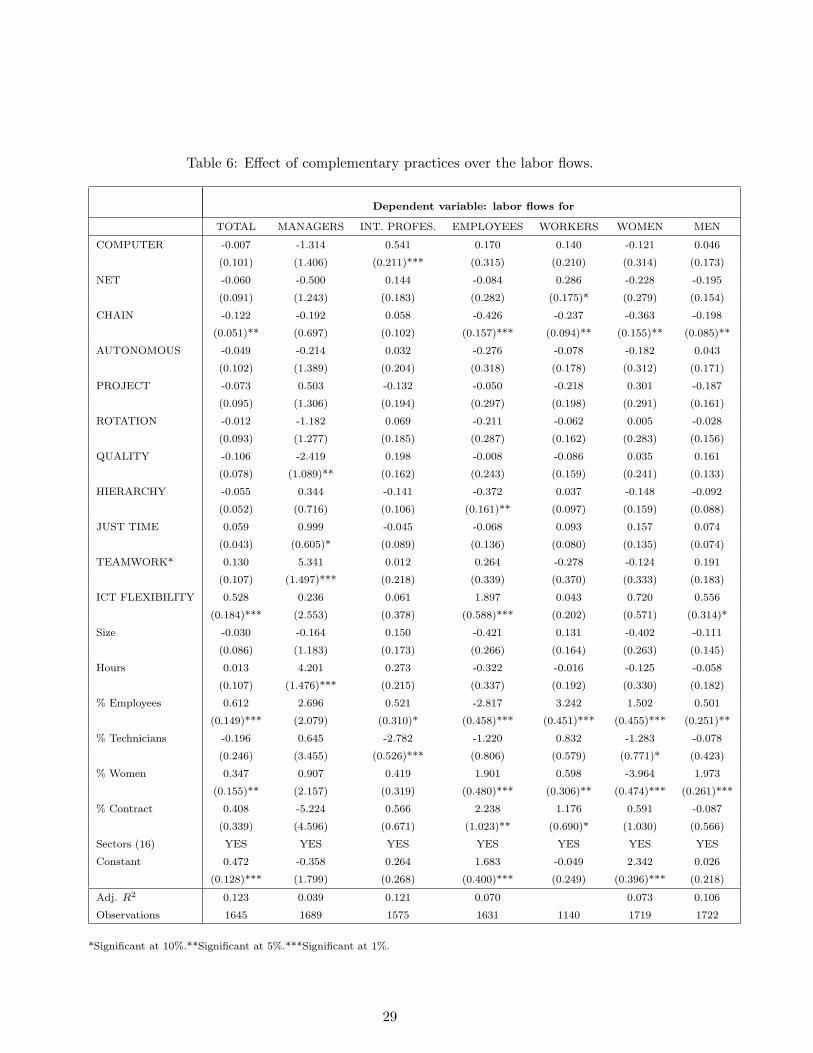
Table 6: Effect of complementary practices over the labor flows.

Dependent variable: labor flows for

TOTAL MANAGERS INT. PROFES. EMPLOYEES WORKERS WOMEN MEN

COMPUTER -0.007 -1.314 0.541 0.170 0.140 -0.121 0.046

(0.101) (1.406) (0.211)*** (0.315) (0.210) (0.314) (0.173)

NET -0.060 -0.500 0.144 -0.084 0.286 -0.228 -0.195

(0.091) (1.243) (0.183) (0.282) (0.175)* (0.279) (0.154)

CHAIN -0.122 -0.192 0.058 -0.426 -0.237 -0.363 -0.198

(0.051)** (0.697) (0.102) (0.157)*** (0.094)** (0.155)** (0.085)**

AUTONOMOUS -0.049 -0.214 0.032 -0.276 -0.078 -0.182 0.043

(0.102) (1.389) (0.204) (0.318) (0.178) (0.312) (0.171)

PROJECT -0.073 0.503 -0.132 -0.050 -0.218 0.301 -0.187

(0.095) (1.306) (0.194) (0.297) (0.198) (0.291) (0.161)

ROTATION -0.012 -1.182 0.069 -0.211 -0.062 0.005 -0.028

(0.093) (1.277) (0.185) (0.287) (0.162) (0.283) (0.156)

QUALITY -0.106 -2.419 0.198 -0.008 -0.086 0.035 0.161

(0.078) (1.089)** (0.162) (0.243) (0.159) (0.241) (0.133)

HIERARCHY -0.055 0.344 -0.141 -0.372 0.037 -0.148 -0.092

(0.052) (0.716) (0.106) (0.161)** (0.097) (0.159) (0.088)

JUST TIME 0.059 0.999 -0.045 -0.068 0.093 0.157 0.074

(0.043) (0.605)* (0.089) (0.136) (0.080) (0.135) (0.074)

TEAMWORK* 0.130 5.341 0.012 0.264 -0.278 -0.124 0.191

(0.107) (1.497)*** (0.218) (0.339) (0.370) (0.333) (0.183)

ICT FLEXIBILITY 0.528 0.236 0.061 1.897 0.043 0.720 0.556

(0.184)*** (2.553) (0.378) (0.588)*** (0.202) (0.571) (0.314)*

Size -0.030 -0.164 0.150 -0.421 0.131 -0.402 -0.111

(0.086) (1.183) (0.173) (0.266) (0.164) (0.263) (0.145)

Hours 0.013 4.201 0.273 -0.322 -0.016 -0.125 -0.058

(0.107) (1.476)*** (0.215) (0.337) (0.192) (0.330) (0.182)

% Employees 0.612 2.696 0.521 -2.817 3.242 1.502 0.501

(0.149)*** (2.079) (0.310)* (0.458)*** (0.451)*** (0.455)*** (0.251)**

% Technicians -0.196 0.645 -2.782 -1.220 0.832 -1.283 -0.078

(0.246) (3.455) (0.526)*** (0.806) (0.579) (0.771)* (0.423)

% Women 0.347 0.907 0.419 1.901 0.598 -3.964 1.973

(0.155)** (2.157) (0.319) (0.480)*** (0.306)** (0.474)*** (0.261)***

% Contract 0.408 -5.224 0.566 2.238 1.176 0.591 -0.087

(0.339) (4.596) (0.671) (1.023)** (0.690)* (1.030) (0.566)

Sectors (16) YES YES YES YES YES YES YES

Constant 0.472 -0.358 0.264 1.683 -0.049 2.342 0.026

(0.128)*** (1.799) (0.268) (0.400)*** (0.249) (0.396)*** (0.218)

Adj. R2 0.123 0.039 0.121 0.070 0.073 0.106

Observations 1645 1689 1575 1631 1140 1719 1722

*Significant at 10%.**Significant at 5%.***Significant at 1%.

29

net technologies explains the increased labor flows. In this case, the potential complemen-

tarities among technological and organizational variables are not significant.

To sum up, complementarities among HPWO practices (TEAMWORK*) or among technological

and organizational practices (ICT FLEXIBILITY) must also be considered when analyzing labor

flows issues. More particularly, the combination of ICT and flexible job assignment practices

has led to a higher aggregate job instability (TOTAL, MEN and EMPLOYEES). In contrast,

the combination of HPWO practices (TEAMWORK*) has mainly affected managers.

6 Conclusion

The main objective of this paper was to bring some light to one aspect for which the existent

literature is not very abundant: the effect of ICT and HPWO practices on job stability (labor

flows). We develop an empirical analysis based on a French database and covering more than

twenty-five hundred establishments. Our estimations reveal that at the aggregate level, labor

flows of all workers are accelerated by the combination of flexible job assignment practices and

ICT. In contrast, the traditional systems of production (chain production systems) reduce the

labor flows. In terms of job categories, we conclude that the labor flows of managers are stimu-

lated by HPWO practices (more particularly by the presence of just in time production systems,

reduction of hierarchical levels, autonomous teams of production or multidisciplinary groups)

while new technologies accelerate labor flows of intermediate professionals, manual workers and

employees. For the last ones, complementarities between ICT and flexible job assignment prac-

tices have been a key determinant in the increased job instability.

In order to provide a structure to these empirical results, we also develop a very simple theoretical

model inspired in Cahuc and Postel-Vinay (2002). The comparative static analysis of the model

reproduces the econometric estimations. That is, any technological or organizational change

improving the relative productivity of one type of job will tend to reduce its turnover and

increase the turnover of the other jobs.

30

References

Abowd, J., and F. Kramarz. 2003. “The Costs of Hiring and Separations.” Labour Economics

10 (5): 499–530.

Askenazy, P., and C. Gianella. 2000. “Le Paradoxe de Productivite: les Changements Or-

ganisationnels, facteur complementaire a l’informatisation.” Economie et Statistique 9/10

(339-340): 219–242.

Bauer, T. 2004. “High Performance Workplace Practices and Job Satisfaction: Evidence from

Europe.” IZA Working Paper, pp. 1–33.

Bauer, T., and S. Bender. 2002. “Technological Change, Organizational Change, and Job

Turnover.” IZA Discussion Paper, no. 570 (September).

Berman, E., J. Bound, and Z. Griliches. 1994. “Changes in the demand for skilled labor

within U.S. manufacturing: evidence from the Annual Survey of Manufacturers.” Quarterly

Journal of Economics 109:367–397.

Bresnahan, T.F., E. Brynjolfsson, and L.M. Hitt. 2002. “Information Technology, Workplace

organization, and the Demand for skilled Labor: Firm-Level Evidence.” The Quarterly

Journal of Economics 117 (1): 339–376.

Burgess, S.M., J. Lane, and D. Stevens. 2000. “Job Flows , Worker Flows, and Churning.”

Journal of Labor Economics 18 (3): 473–502 (July).

Burgess, S.M., and S. Nickell. 1990. “Labour Turnover in UK Manufacturing.” Economica 57

(227): 295–317 (August).

Cahuc, P., and F. Postel-Vinay. 2002. “Temporary Jobs, Employment Protection and Labor

Market Performance.” Labour Economics 9:63–91.

Cappelli, P. 1996. “Technology and Skill Requirements: Implications for Establishment Wage

Structures.” New England Economic Review, pp. 139–154.

Caroli, E., and J. Van Reenen. 2001. “Skilled Biased Technological Change? Evidence from

a Pannel of British and French Establishments.” Quarterly Journal of Economics 116 (4):

1449–1492.

31

Fitz Roy, F., and M. Funke. 1995. “Capital Skill Complementarity in West German Manufac-

turing.” Empirical Economics 20:651–665.

Givord, P., and E. Maurin. 2004. “Changes in job security and their causes: An empirical

analysis for France, 1982-2002.” European Economic Review 48 (3): 595–615 (June).

Greenan, N. 1996. “Progres Technique et Changements Organisationnels: leur Impact sur

l’Emploi et les Qualifications.” Economie et Statistique CCXCVIII:35–44.

Hamermesh, D., W.H.J. Hassink, and J.C. Van-Ours. 1996. “Job Turnover and Labor Turnover:

A Taxonomy of Employment Dynamics.” Annales d’Economie et de Statistique 41/42:21–

39.

Ichniowski, C., K. Shaw, and G. Prennushi. 1997. “The Effects of Human Resource Man-

agement Practices on Productivity: A Study of Steel Finishing Lines.” The American

Economic Review 87 (3): 291–313 (June).

Jones, D.C., T. Kato, and A. Weinberg. 2003, September. Low Wage in America. Edited

by E. Appelbaum, A. Bernhardt, and R.J. Murnane. Russell Sage Foundation. Chapter

13: Managerial Discretion, Business Strategy, and the Quality of Jobs: Evidence from

Medium-Sized Manufacturing Establishments in Central New York.

Krusell, P., L.E. Ohanian, J.V. Rios-Rull, and G.L. Violante. 2000. “Capital skill complemen-

tarity and inequality: A macroeconomic analysis.” Econometrica 68 (5): 1029–53.

Machin, S., A. Ryan, and J. Van Reenen. 1998. “Technology and changes in skill structure:

Evidence from seven OECD countries.” Quarterly Journal of Economics 113:1215–44.

Michelacci, C., and D. Lopez-Salido. 2004. “Technology Shocks and Job Flows.” mimeo.

Moreno-Galbis, E. 2002. “Causes of the Change in the Skill Structure of the Labour Force:

An Empirical Application to the Spanish case.” IRES Dicussion Paper, no. No. 35.

Mortensen, D., and C.A. Pissarides. 1994. “Job Creation and Job Destruction in the Theory

of Unemployment.” Review of Economic Studies 61:397–415.

Neumark, D., D. Polsky, and D. Hansen. 1999. “Has Job Stability Declined Yet? New Evidence

for the 1990s.” Journal of Labor Economics 4, no. S29-S64 (October).

32

Neumark, D., and D. Reed. 2004. “Employment Relationships in the New Economy.” Labour

Economics 11 (1): 1–31 (February).

OECD. 1996, July. “OECD Employment Outlook.” Technical Report, OECD.

Pissarides, C. 1990. Equilibrium Unemployment Theory. Edited by MIT Press. Cambridge,

Massachusetts: MIT Press.

Valletta, R.D. 1999. “Declining Job Security.” Journal of Labor Economics 17 (4): S170–S197.

33

Appendix 1: Steady State.

At the equilibrium the firms open vacancies until no more benefit can be obtained, that is, all

rents are exhausted and the free entry condition applies: Πvc= 0 and Πvs

= 0. From equations

(5), (6), (7) and (8) we derive the following expressions for each period:

ac

β(1− η) q(θc)=

∫ ε

εMax[Sc(x), 0] dΦ(x) , (24)

as

β(1− η) q(θs)=

∫ ε

εMax[Ss(x), 0] dΦ(x) . (25)

We notice, that all jobs contacts will not lead to a job creation since, once the contact is made

and the idiosyncratic productivity revealed, both parties may realize that the match is not

productive enough to compensate for the search and hiring efforts. A contact will become a

productive match if and only if the joint surplus (the one obtained by the firm plus the one of

the worker) is positive. Therefore, for each type of job there exists a a critical productivity level,

εc and εs, such that Sc(εc) = 0 and Ss(εs) = 0. Below these reservation productivity levels the

joint surplus is negative and it is not profitable to create or continue a job.

To compute εc and εs, we first define the joint surplus of both types of jobs using equations

(5)-(14) as well as the free entry conditions, (24) and (25):

Sc(ε) = ε + h1 − wu + β(1− λ)Max[Sc(ε), 0] + βλ

∫ ε

εMax[Sc(x), 0]dΦ(x)− ηacθc

1− η,(26)

Ss(ε) = ε + h2 − wu + β(1− λ)Max[Ss(ε), 0] + βλ

∫ ε

εMax[Ss(x), 0]dΦ(x)− ηasθs

1− η.(27)

At the threshold values εc and εs, equations (26) and (27) respectively become zero leading to:

η ac θc

1− η= εc + h1 − wu + β λ

∫ ε

εc

Sc(x) dΦ(x) , (28)

η as θs

1− η= εs + h2 − wu + β λ

∫ ε

εs

Ss(x) dΦ(x) . (29)

From (26) and (27) we know that S′ c = 11−β(1−λ) > 0 and S′ s = 1

1−β(1−λ) > 0. Using these

results and integrating by parts the integrals in (28) and (29) permits to determine the complex

and simple job destruction rule:

η ac θc

1− η= εc + h1 − wu +

β λ

1− β(1− λ)

∫ ε

εc

(1− Φ(x)) dx , (30)

η as θs

1− η= εs + h2 − wu +

β λ

1− β(1− λ)

∫ ε

εs

(1− Φ(x)) dx . (31)

34

Whether we consider the complex or the simple segment of the labor market we observe a positive

relationship between the market tightness of the corresponding segment and its reservation

productivity (see proof bellow). Therefore, the job destruction curves of the complex and simple

segment of the labor market are positively sloped in the space (θc, ε) and (θs, ε), respectively.

Proof.

We analyze the slope of the job destruction curve for the complex segment of the labor market,

but the procedure is identical for the simple segment.

η ac

1− η

dθc

dεc= 1 +

β λ

1− β(1− λ)d

dεc

∫ ε

εc

(1− Φ(x))dx , (32)

= 1 +β λ

1− β(1− λ)

(− d

dεc

∫ εc

ε(1− Φ(x))dx

),

= 1− β λ

1− β(1− λ)(1− Φ(εc)) .

From the previous expression we realize that:

signdθc

dεc= sign

(1− β λ

1− β(1− λ)(1− Φ(εc))

)(33)

We proceed then to determine the sign of the right hand side of equation (33). Because 0 < β < 1

we know that 1− β + β λ > β λ. Therefore:

0 <β λ

1− β(1− λ)< 1 .

At the same time, since Φ(x) is a probability distribution function we know that 0 ≤ 1−Φ(εc) ≤1. Multiplying two numbers smaller than one leads to a positive number smaller than one,

therefore:

1− β λ

1− β(1− λ)(1− Φ(εc)) > 0 which implies

dθc

dεc> 0 . (34)

The job destruction curve in the complex segment is positive sloped. The positivity of the slope

in the simple segment can be determined in a similar way. ¥

35

We apply on equations (24) and (25) the same procedure developed to compute (30) and (31)

so as to determine the job creation rule of each type of firm:

ac

β(1− η) q(θc)=

11− β(1− λ)

∫ ε

εc

(1− Φ(x)) dx , (35)

as

β(1− η) q(θs)=

11− β(1− λ)

∫ ε

εs

(1− Φ(x)) dx , (36)

We prove now that both equations determine a negative relationship between market tightness

and ε, meaning that the job creation curves are negatively sloped in the space (θi, ε) for i = c, s.

Proof.

We develop the proof for the complex case but, here again, the same procedure applies for the

simple segment.

− ac

β (1− η)q′(θc)q2(θc)

dθc

dεc=

11− β(1− λ)

d

dεc

∫ ε

εc

(1− Φ(x))dx , (37)

− ac

β (1− η)q′(θc)q2(θc)

dθc

dεc= − 1

1− β(1− λ)d

dεc

∫ εc

ε(1− Φ(x))dx ,

ac

β (1− η)q′(θc)q2(θc)

dθc

dεc=

11− β(1− λ)

(1− Φ(εc)) .

Because 0 < β < 1, 0 < η < 1 and ac > 0 the first term on the left hand side, ac

β (1−η) , is positive.

At the same time, since 0 < λ < 1 and Φ(x) is a probability distribution function, the right

hand part of equation (37) is positive. Therefore:

signdθc

dεc= sign

q2(θc)q′(θc)

(38)

As q2(θc) is always positive and the probability of filling a vacancy is a decreasing function

on the labor market tightness (q′(θc) < 0), we find that q2(θc)q′(θc) < 0. The job creation curve is

negatively sloped. ¥

Finally, substituting the value functions into the surplus sharing rules (5) and (6) we obtain the

following expression for the wages (see Pissarides (1990) chapter 2):

wc = (1− η) wu + η(ε + h1 + acθc) , (39)

ws = (1− η) wu + η(ε + h2 + asθs). (40)

36

Appendix 2: Original regressions

The variables included in the estimations of equation (19) (tables 3 and 4), have been chosen

after successively eliminating the least significant variables among the following:

1. Explicative variables

• COMPUTER: Dummy variable taking the value 1 if 50% or more workers use a

computer.

• NET: Dummy variable taking the value 1 if between 20 and 50% of the workers use

the net system.

• INTERNET: Dummy variable taking the value 1 if between 20 and 50% of the workers

use the internet.

• CHAIN: Dummy variable taking the value 1 when the establishment still uses systems

of tayloristic production systems (robots, computer assisted systems, etc.).

• AUTONOMOUS: Dummy variable taking the value 1 if between 20 and 50% of the

workers participate in autonomous teams of production.

• PROJECT: Dummy variable taking the value 1 if between 20 and 50% of the workers

participate in multidisciplinary working groups or project groups.

• ROTATION: Dummy variable taking the value 1 when a majority of workers rotates

among tasks inside the firm.

• QUALITY: Dummy variable taking the value 1 when the establishment develops a

total quality control procedure.

• HIERARCHY: Dummy variable taking the value 1 when the establishment has re-

duced the number of hierarchical levels.

• JUST TIME: variable taking the value 1 when the establishment practices the just

in time production methods either with the customer or with the supplier.

2. Control variables:

• Tech. change: Dummy variable taking the value 1 if in 1998 there has been an

important technological change in the establishment.

37

Table 7: Determinants of labor flows for different categories of workers.TOTAL MANAGERS INT. PROFES. EMPLOYEES WORKERS WOMEN MEN

COMPUTER 0.111 -1.069 0.252 0.632 0.086 0.079 0.188(0.102) (1.417) (0.209) (0.317)** (0.181) (0.314) (0.173)

NET -0.027 0.032 0.024 -0.040 0.339 -0.225 -0.118(0.095) (1.305) (0.190) (0.296) (0.165)** (0.291) (0.161)

INTERNET -0.171 -0.223 -0.225 0.070 -0.557 0.234 -0.410(0.167) (2.307) (0.336) (0.531) (0.351)* (0.513) (0.283)

CHAIN -0.094 -0.298 0.053 -0.221 -0.193 -0.346 -0.159(0.057)* (0.781) (0.113) (0.176) (0.097)* (0.174)* (0.095)

AUTONOMOUS 0.029 2.177 0.084 -0.158 -0.024 -0.226 0.134(0.090) (1.238)* (0.180) (0.282) (0.147) (0.277) (0.152)

PROJECT -0.000 2.678 -0.248 0.077 -0.201 0.261 -0.080(0.088) (1.216)** (0.178) (0.275) (0.151) (0.270) (0.149)

ROTATION 0.115 -1.404 0.132 0.321 -0.120 0.165 0.116(0.082) (1.145) (0.166) (0.258) (0.136) (0.253) (0.139)

QUALITY -0.110 -2.597 0.191 -0.007 -0.075 0.106 0.154(0.080) (1.111)** (0.164) (0.247) (0.143) (0.245) (0.135)

HIERARCHY -0.050 0.732 -0.160 -0.326 0.050 -0.143 -0.082(0.052) (0.718) (0.105) (0.161)** (0.089) (0.159) (0.088)

JUST TIME 0.065 1.098 -0.041 -0.067 0.075 0.185 0.068(0.044) (0.613)* (0.089) (0.138) (0.074) (0.136) (0.075)

Tech. change -0.083 -1.065 0.137 -0.007 -0.283 0.139 0.006(0.091) (1.251) (0.182) (0.281) (0.163)* (0.278) (0.154)

Variation -0.027 -0.366 -0.062 -0.003 -0.013 -0.236 0.074(0.084) (1.163) (0.171) (0.259) (0.146) (0.257) (0.142)

Increasing 0.043 -1.124 0.269 -0.114 0.271 0.437 0.087(0.404) (4.919) (0.798) (1.083) (0.598) (1.098) (0.626)

Decreasing 0.247 2.596 0.515 -0.220 0.138 0.347 0.509(0.411) (5.033) (0.813) (1.110) (0.611) (1.123) (0.639)

Stable 0.148 -1.154 0.158 -0.341 0.329 0.463 0.057(0.405) (4.923) (0.800) (1.085) (0.600) (1.100) (0.627)

Size 0-50 -0.003 0.683 0.352 -0.543 -0.162 -0.642 -0.132(0.392) (5.278) (0.843) (1.164) (0.718) (1.179) (0.629)

Size 50-500 -0.000 0.218 0.128 -0.418 0.033 -0.396 -0.127(0.095) (1.314) (0.192) (0.294) (0.160) (0.291) (0.160)

Size +500 0.094 1.044 0.018 0.035 -0.143 0.011 0.004(0.080) (1.102) (0.161) (0.246) (0.137) (0.244) (0.135)

Hours 0.005 3.898 0.275 -0.202 -0.042 -0.173 -0.029(0.109) (1.493)*** (0.215) (0.339) (0.180) (0.332) (0.183)

% Employees 0.580 3.591 0.843 -3.902 2.400 1.248 0.353(0.176)*** (2.451) (0.362)** (0.534)*** (0.397)*** (0.532)** (0.294)

% Technicians -0.232 0.226 -2.820 -1.762 1.016 -1.428 -0.146(0.255) (3.574) (0.536)*** (0.827)** (0.504)** (0.792)** (0.436)

% Managers 0.077 -2.318 2.734 -0.855 0.363 -0.680 0.058(0.312) (4.323) (0.651)*** (0.977) (0.689) (0.956) (0.527)

% Women 0.354 1.097 0.363 1.925 0.644 -4.613 2.083(0.168)** (2.341) (0.344) (0.517)*** (0.294)** (0.512)*** (0.282)***

% Contract 0.464 -3.630 0.856 1.997 1.261 0.596 -0.034(0.346) (4.690) (0.680) (1.040)* (0.587)** (1.045) (0.575)

AgricultureFood industry -0.307 1.630 -6.254 -0.738 1.291 0.975 0.593

(0.406) (5.472) (0.967)*** (1.209) (0.852) (1.171) (0.659)Consumption industry -0.528 0.736 -6.289 -0.930 0.927 1.425 0.294

(0.397) (5.376) (0.958)*** (1.186) (0.846) (1.164) (0.645)Car industry -0.572 1.061 -6.127 -0.621 1.167 0.130 0.543

(0.441) (5.986) (1.028)*** (1.339) (0.895) (1.277) (0.722)Equipment industry -0.427 1.869 -6.262 -0.272 0.988 0.256 0.620

(0.401) (5.398) (0.958)*** (1.195) (0.852) (1.145) (0.650)Intermediary industry -0.511 1.485 -6.252 -0.540 1.123 0.300 0.522

(0.395) (5.304) (0.950)*** (1.172) (0.842) (1.125) (0.637)Energy -0.584 1.637 -6.134 -0.059 3.947 0.745

(0.517) (7.021) (1.150)*** 1.629 (1.019)*** (0.854)Building -0.415 1.647 -6.116 -0.224 1.165 -0.363 0.898

(0.414) (5.582) (0.978)*** (1.248) (0.861) (1.188) (0.672)Trade -0.389 0.068 -6.393 1.151 1.187 1.073 0.797

(0.391) (5.230) (0.941)*** (1.149) (0.842) (1.147) (0.626)Transport -0.333 1.304 -6.312 -0.086 1.208 0.028 0.795

(0.413) (5.502) (0.979)*** (1.210) (0.852) (1.191) (0.661)Finance -0.545 1.862 -6.370 1.075 -0.767 2.018 -0.012

(0.429) (5.735) (1.011)*** (1.271) (1.123) (1.258) (0.690)Housing -0.573 -6.215 0.556 1.315

(0.510) (1.172)*** (1.054) (1.546)Services firms 0.127 1.644 -6.151 0.077 1.237 1.618 0.945

(0.395) (5.321) (0.954)*** (1.170) (0.859) (1.157) (0.637)Services individuals 1.353 21.549 -4.852 4.953 2.173 4.580 3.187

(0.435)*** (5.924)*** (1.020)*** (1.291)*** (0.988)** (1.292)*** (0.705)***Education -0.127 -0.168 -3.792 1.644 -0.250 3.676 0.481

(0.392) (5.317) (0.946)*** (1.168) (0.832) (1.184)*** (0.635)Administration 1.407 2.371 1.822 1.949

(6.931) (1.540) (1.523) (0.829)**Constant 0.700 -1.823 6.060 1.983 -1.342 1.434534 -0.833

(0.571) (7.235) (1.250)*** (1.592) (1.032) (1.593) (0.889)

*Significant at 10%.**Significant at 5%.***Significant at 1%.

38

• Variation: Dummy variable taking the value 1 if the economic activity of the estab-

lishment has suffered an unusual variation in 1998.

• Increasing: Dummy variable taking the value 1 if the economic activity of the estab-

lishment has been increasing in 1998.

• Decreasing: Dummy variable taking the value 1 if the economic activity of the estab-

lishment has been decreasing in 1998.

• Stable: Dummy variable taking the value 1 if the economic activity of the establish-

ment has remained stable in 1998.

• Size 0-50: Dummy variable taking the value 1 if the number of workers in the firm is

lower than 50.

• Size 50-500: Dummy variable taking the value 1 if the number of workers in the firm

is between 50 and 500.

• Size +500: Dummy variable taking the value 1 if the number of workers in the firm

is above 500.

• Hours: Dummy variable taking the value 1 if the firm has already implemented the

reduction in the number of working hours.

• % Employees, % Technicians and % Managers are the percentage of employees, tech-

nicians and managers in the firm.

• % Women is the percentage of women in the firm.

• % Contract is the percentage of fixed duration contract in the firm.

• We control for the following economic sectors: agriculture and fishing (Agriculture);

agricultural and food industry (Food industry); consumption industry (Consump-

tion industry), automobile industry (Car industry); equipment industry (Equipment

industry); intermediary goods’ industry (Intermediary industry); energy sector (En-

ergy); building sector (Building); trade sector (Trade); financial activity sector (Fi-

nance); housing activities (Housing); services to firms (Services firms); services to

individuals (Services individuals); education, health and social action (Education);

and administration (Administration).

39

Appendix 3: Means and standard deviations

Table 8: Mean and standard deviation of variables in cross section analysis.

Variables Mean Standard deviationTOTAL 0.741 2.213MANAGERS 0.764 18.800INT. PROFES. 0.697 2.835EMPLOYEES 0.921 4.323WORKERS 0.574 2.149WOMEN 1.081 4.338MEN 0.845 2.536COMPUTER 0.317 0.465NET 0.252 0.434CHAIN 0.778 0.805AUTONOMOUS 0.192 0.394PROJECT 0.244 0.430ROTATION 0.251 0.433QUALITY 0.606 0.489HIERARCHY 0.924 0.726JUST TIME 0.708 0.846Size 0.189 0.392Hours 0.106 0.308% Employees 0.314 0.322% Technicians 0.162 0.162% Women 0.380 0.284% Contract 0.058 0.114Energy 0.007 0.086Building 0.058 0.233Finance 0.036 0.186Services firms 0.101 0.301Services individuals 0.0439 0.205Education 0.126 0.332Administration 0.013 0.115

40

Appendix 4: Correlation matrix

Table 9: Correlation matrix.TOTAL MANAGERS INT. PROFES. EMPLOYEES WORKERS WOMEN MEN

TOTAL 1.000

MANAGERS 0.214 1.000(0.000)

INT. PROFES. 0.224 -0.003 1.000(0.000) (0.887)

EMPLOYEES 0.452 -0.001 0.199 1.000(0.000) (0.959) (0.000)

WORKERS 0.270 0.036 0.089 0.160 1.000(0.000) (0.187) (0.001) (0.000)

WOMEN 0.348 0.016 0.190 0.212 0.151 1.000(0.000) (0.516) (0.000) (0.000) (0.000)

MEN 0.727 0.301 0.444 0.486 0.251 0.272 1.000(0.000) (0.000) (0.000) (0.000) (0.000) (0.000)

COMPUTER 0.031 -0.016 -0.004 0.023 0.075 -0.026 0.014(0.163) (0.481) (0.854) (0.337) (0.005) (0.249) (0.525)

NET -0.044 -0.015 -0.024 -0.023 0.073 -0.057 -0.060(0.049) (0.533) (0.320) (0.328) (0.007) (0.012) (0.007)

CHAIN -0.149 -0.028 -0.122 -0.116 -0.118 -0.117 -0.152(0.000) (0.234) (0.000) (0.000) (0.000) (0.000) (0.000)

AUTONOMOUS -0.042 0.046 -0.039 -0.031 -0.047 -0.032 -0.013(0.056) (0.049) (0.108) (0.193) (0.079) (0.153) (0.557)

PROJECT -0.023 0.039 0.002 0.007 -0.037 0.008 -0.010(0.304) (0.092) (0.932) (0.765) (0.166) (0.717) (0.666)

ROTATION -0.029 -0.014 -0.039 0.001 -0.058 -0.020 -0.014(0.191) (0.540) (0.102) (0.982) (0.033) (0.380) (0.541)

QUALITY -0.103 -0.037 -0.045 -0.046 -0.058 -0.033 -0.034(0.000) (0.113) (0.063) (0.049) (0.031) (0.147) (0.128)

HIERARCHY -0.043 0.032 -0.101 -0.080 -0.028 -0.048 -0.064(0.051) (0.173) (0.000) (0.001) (0.300) (0.033) (0.004)

JUST TIME -0.039 0.032 -0.0890 -0.058 -0.033 -0.040 -0.057(0.081) (0.172) (0.000) (0.013) (0.223) (0.078) (0.011)

COMPUTER NET CHAIN AUTONOMOUS PROJECT ROTATION QUALITY

COMPUTER 1.000

NET 0.496 1.000(0.000)

CHAIN -0.012 0.086 1.000(0.531) (0.000)

AUTONOMOUS -0.038 0.036 0.171 1.000(0.042) (0.056) (0.000)

PROJECT 0.184 0.204 0.061 0.153 1.000(0.000) (0.000) (0.001) (0.000)

ROTATION -0.107 -0.049 0.134 0.098 -0.004 1.000(0.000) (0.010) (0.000) (0.000) (0.822)

QUALITY -0.004 0.061 0.317 0.159 0.100 0.095 1.000(0.841) (0.001) (0.000) (0.000) (0.000) (0.000)

HIERARCHY 0.075 0.136 0.249 0.117 0.144 0.061 0.209(0.000) (0.000) (0.000) (0.000) (0.000) (0.001) (0.000)

JUST TIME -0.081 -0.002 0.316 0.135 0.007 0.169 0.242(0.000) (0.931) (0.000) (0.000) (0.696) (0.000) (0.000)

HIERARCHY

HIERARCHY 1.000

JUST TIME 0.210 1.000(0.000)

() Significance levels.

41