The Impact of Sprawl on Commuting in Alabama

By

Joe Weber Department of Geography

University of Alabama Tuscaloosa, Alabama

And

Selima Sultana Department of Geography

University of North Carolina at Greensboro Greensboro, North Carolina

Prepared by

UTCA University Transportation Center for Alabama The University of Alabama, The University of Alabama at Birmingham,

and The University of Alabama at Huntsville

UTCA Report 04108 June 14, 2005

ii

Technical Report Documentation Page

1. Report No

2. Government Accession No. 3. Recipient Catalog No.

5. Report Date May 31, 2005

4. Title and Subtitle The Impact of Sprawl on Commuting in Alabama

6. Performing Organization Code

7. Authors Joe Weber and Selima Sultana

8. Performing Organization Report No.

10. Work Unit No.

9. Performing Organization Name and Address Department of Geography The University of Alabama Tuscaloosa, AL, and Greensboro Department of Geography University of North Carolina-Greensboro Greensboro, NC

11. Contract or Grant No. DTSR0023424

13. Type of Report and Period Covered Final Report 1/1/2004 – 4/30/2005

12. Sponsoring Agency Name and Address University Transportation Center for Alabama The University of Alabama Box 870205, Tuscaloosa, AL 35487

14. Sponsoring Agency Code

15. Supplementary Notes 16. Abstract This research examines the influence and importance of urban sprawl on commuting patterns within Birmingham and Tuscaloosa, Alabama. Geographic Information Systems -based methodologies were used to define and map urban sprawl, with the 2000 Census Transportation Planning Package as the primary dataset. The results confirmed that workers living in sprawl areas commute farther to work in both mileage and travel time than those living in older, higher density areas of the city. Workers who commute into urban areas from outlying sprawl zones have the longest commutes, while those who commute entirely within the city have the shortest. This suggests that as residences continue to move to sprawl areas commuting times can be expected to greatly increase as workers journey to urban jobs. However, as jobs continue to move to sprawling areas, commuting times may decrease due to an increase of shorter within-sprawl commuting. Increasing sprawl could therefore lead to an equalization of commuting times. 17. Key Words

18. Distribution Statement

19. Security Class (of report)

20. Security Class . (Of page) 21. No of Pages

22. Price

FORM F1700.7

iii

Contents

Contents……………………………………………………………………………………. iii Tables………………………………………………………………………………………. iv Figures……………………………………………………………………………………… iv Executive Summary………………………………………………………………………… v 1.0 Introduction…………………………………………………………………………….. 1 2.0 Background……………………………………………………………………………... 2

Sprawl Definitions………………………………………………………………..… 2 Mapping Sprawl…………………………………………………………………….. 4 Sprawl and Commuting…………………………………………………………..… 4

3.0 Data and Methodology……………………………………………………………….… 6 4.0 Results………………………………………………………………………….……….. 8

Mapping Sprawl Areas………………………………………………………………8 Sprawl and Commuting Patterns…………………………………………………….9 Home and Job Locations………………………………………………………….…10

5.0 Conclusions and Recommendations………………………………………………….…13

Generalizations about Sprawl and Commuting……………………………………..13 Planning Implications………………………………………………………….……14 Applicability to Other Areas……………………………………………………….. 15 Recommendations for Further Work………………………………………….…….15

6.0 References…………………………………………………………………………….…17

iv

List of Tables Number Page 4-1 Commuting differences between sprawl and urban areas………………………. 10 4-2 Commuting patterns in Birmingham……………………………………….……. 11 4-3 Commuting patterns in Tuscaloosa…………………………………………..….. 12

List of Figures Number Page 1-1 Sprawl at the metropolitan level……………………………………………….….. 2 1-2 Sprawl in Alabama……………………………………………………………..…. 3 4-1 Sprawl in Birmingham and Tuscaloosa…………………………………………… 8

v

Executive Summary

It is well known that in many cities considerable population growth is occurring outside the urban core area, with very low densities of residential and commercial activity in surrounding areas. This condition is often known as urban sprawl and has been subject to a wide range of criticism for its wasteful use of land, increased traffic congestion and lengthened travel required by residents. However, the effects of this sprawl remain largely in the realm of qualitative judgments. The objective of this research was to identify the influence and importance of urban sprawl on commuting patterns within Alabama cities, using the Birmingham and Tuscaloosa metropolitan areas as study areas. The commuting times and distances of residents from sprawl and urban were compared to determine the significance and magnitude of sprawl impacts. Geographic Information Systems-based methodologies were used to define and map urban sprawl. The 2000 Census Transportation Planning Package was used as the primary dataset. This allows commuting times and distances to be identified for workers in different areas, allowing comparisons between sprawl and urban areas. It also allows determination of the locations of jobs associated with commuting patterns. The results confirmed that workers living in sprawl areas commute farther to work in both mileage and travel time than those living in older, higher density areas of the city. However, transit, biking and walking times generally do not vary between sprawling and urban areas. The research provides important insights into the importance of sprawl locations on the relationships between home and work. Workers who commute into urban areas from outlying sprawl zones have the longest commutes, while those who commute entirely within the city have the shortest. This suggests that as residences continue to move to sprawl areas commuting times can be expected to greatly increase as workers journey to urban jobs. As jobs continue to move to sprawling areas, commuting times may decrease due to an increase of shorter within-sprawl commuting (even if within-sprawl commuting is not quite as short as within-urban commuting). Increasing sprawl could therefore lead to an equalization or even reduction of commuting times, suggesting that sprawl may have important benefits in additional to the more commonly mentioned costs.

1

Section 1 Introduction

It is well known that in most cities and towns growth is occurring outside the urban core area, with very low densities of residential and commercial activity in surrounding areas. This condition is often known as urban sprawl and has been subject to a wide range of criticism, including for its negative effects on travel behavior and commuting. Residents of sprawl areas may drive longer distances to more dispersed destinations, be more reliant on automobiles due to a lack of transit service and limited opportunities for biking or walking, and contribute unnecessarily to air pollution and congestion. Unfortunately, there is little agreement about what constitutes sprawl. One review identified several ways of talking about sprawl (Galster, et al 2001). One of the most common is to hear of sprawl as a stereotype or common form of growth found in a particular area, such as Los Angeles. Sprawl is also often defined as any growth considered ugly, such as commercial strips. It may be seen as the outcome of poor planning, or as the cause of congestion or increased pollution. Sprawl may be defined as a low-density urban pattern, or as a particular urban growth process. Additionally, sprawl is increasingly used to describe any urban growth (as in Chapman and Lund 2004; Crane and Chatman 2004; Gutfreund 2004; Wolch, Pastor, and Dreier 2004). Expectations about the relationships between sprawl and commuting may vary widely depending on which perspective is used. This project treats sprawl as an urban growth process with high rates of population growth and low densities. This research uses a straightforward definition of sprawl based on growth and density that is implemented using Geographic Information Systems (GIS) and readily-available data. This definition is applied to the Birmingham and Tuscaloosa, Alabama, metropolitan areas. Sprawl is be mapped for these areas and combined with data on commuting to compare how the journey to work differs for residents of sprawl areas versus older and denser urban areas. Prior to this project, it was expected that commuting trips were longer and more automobile dominated for residents of sprawling areas, but this had not been directly tested. This project provided an opportunity to identify how sprawl affects the lives of urban residents in Alabama.

2

Section 2 Background

Sprawl Definitions A number of researchers have constructed quantitative definitions of urban sprawl, usually focusing on counties or Metropolitan Statistical Areas (MSAs, which are areas based on counties defined by the Census Bureau around large cities). A simple approach is to define sprawl as growth located outside a certain radius of the urban center (Kahn 2001). Another approach treats sprawl as previously undeveloped land that experiences high rates of growth (Transportation Research Board 2002). Because the Census Bureau defines an Urbanized Area (UA) around each city, sprawl can be defined as growth that takes place outside this boundary (El Nasser and Overberg 2001). More elaborate measures also used the concentration, continuity, and land use mix of development (Malpezzi 1999; Galster, et al 2001; Ewing, Pendall, and Chen 2004; Hasse and Lathrop 2003; Frumkin, Frank, and Jackson 2004; Tsai 2005). Because these definitions are designed for metropolitan areas, they can be mapped to indicate national sprawl patterns. Figure 1-1 shows one set of sprawl rankings, with higher numbers representing greater sprawl (El Nasser and Overberg 2001). Contrary to popular perception, it shows Los Angeles is not the most sprawling city in the country, but one of the least sprawling.

Figure 1-1. Sprawl at the metropolitan level

3

Instead, sprawl is greatest for many eastern metropolitan areas, with Nashville, Tennessee, and Charlotte, and Greensboro, North Carolina being the three most sprawling large cities. This regional pattern of greater sprawl in the eastern U.S. is not recent, and appears to have existed since at least the 1960s (Lamb 1983). Sprawl exists in Alabama as well (Figure 1-2). The most sprawling city in the state is Mobile, which is the 36th most sprawling metropolitan area in the country. Birmingham was ranked 99th, while Tuscaloosa, the least sprawling metro area in the state, is 229th nationally. With higher rates of population growth these rankings would surely be much higher.

Figure 1-2. Sprawl in Alabama That physical and especially political geography is an important element in reducing the potential for sprawl in many cities has been noted. This is addressed directly by Lang (2003), who finds that Western cities tend to more densely developed. Although Sunbelt metropolitan areas are often fast growing, there are tremendous differences between the “wet” Sunbelt (in the Southeast, typified by cities such as Atlanta and Nashville) and the “dry” Sunbelt (in the Southwest, Nevada, and California, typified by places like Phoenix). National parks, forests, military bases, and Indian reservations limit growth around the peripheries of dry Sunbelt cities, while a monopoly on the provision of municipal services such as water lines also makes for higher density in that area. There is therefore little barrier to the development of a continuously sprawling Piedmont metropolitan area between Raleigh, NC, and Birmingham, AL. There is less chance that cities such as Las Vegas and Los Angeles will sprawl together, partly due to the existence of Mojave National Preserve between them, a park that was created with sprawl prevention in mind (Hamin 2003).

4

Mapping Sprawl Although mapping sprawl for metropolitan areas has been common, there have been few attempts at mapping it within cities. Mapping growth patterns of cities at the rural-urban fringe provides one approach, and presents a detailed view of how cities expand into surrounding lands. In the case of Phoenix, a dry-western Sunbelt metropolis, the process through the 1990s was a very orderly outward expansion, with a fairly narrow area of peak growth (Gober and Burns 2002). This type of growth represents a wave of pushing outwards during real estate booms, which has been characterized as an urban “bow wave” of development (Hart 1991). Growth patterns need not be mapped for standard census statistical units, but can also be mapped for watersheds (Sultana and Chaney 2003) or using raster cells (Weber and Maret 2003). With these approaches the location of sprawl within a metropolitan area can be identified. Mapping at this level is appropriate because “sprawl has different meanings on different spatial scales” (Frumkin, Frank, and Jackson 2004, 5), and the results obtained at the metropolitan scale need to be matched with sprawl at the level of neighborhoods, shopping centers, and commuting patterns.

Sprawl and Commuting In addition to defining the term, attention has focused on the impacts of sprawl. In terms of transportation and travel behavior, the primary argument focuses on high levels of dependence on cars for transportation and greater distances between destinations. Impacts of these could include more and longer daily trips and greater traffic congestion, reducing access to services or jobs (Johnson 2001; Gillham 2002). Spending more time in cars may reduce social contacts with others and could be related to obesity and other health problems (Freeman 2001; Sui 2003; Frumkin, Frank, and Jackson 2004; Kelly-Schwartz, Stockard, Doyle, and Schlossberg 2004). Building roads in low-density environments costs less than in denser urban areas (Carruthers and Ulfarsoon 2003). At the metropolitan level studies linking urban density to commuting times or mileage has become common, with the common result that average commuting lengths have remained surprisingly constant despite substantial increases in urban population and congestion (Gordon, Kumar, and Richardson 1989a, 1989b, Gordon, Richardson, and Jun 1991; Levinson and Kumar 1994, 1997; Crane and Chatman 2004). This “commuting paradox” is explained by the declining importance of traditional downtown employment centers and consequent replacement of long inward commuting trips with potentially shorter trips within suburban areas. It is also expected that workers are relocating their homes to be closer to jobs, thereby preserving conveniently short commuting times. There has been very little research on the relationship between sprawl and commuting at the intraurban level, but the influence of various aspects of urban form (such as density, street configuration, and land use mixes) on travel behavior have been increasingly investigated. This has been motivated by the possibility of using urban design and architecture as a means of altering automobile dominated travel patterns in favor of more balanced use of transit and walking densities (Frank and Pivo 1994; Friedman, Gordon, and Peers 1994). However, because of the range of data and methods that have been used, and the possibility that people will relocate

5

near work, or choose particular residential areas for reasons entirely unrelated to travel choices, relationships between urban form and travel behavior remain uncertain (Berman 1996; Crane 1996; Handy 1996; Crane and Crepeau 1998; Boarnet and Crane 2001). Some work has explicitly examined sprawl at this scale. In the Auburn-Opelika area rapid low-density growth patterns at the watershed level have been found to be associated with longer commutes and greater auto use among residents (Sultana and Chaney 2003). Transit services are unlikely to reach into sprawling areas, and will serve these areas poorly due to lower population densities (Weber and Maret 2003). This research will help fill in the lack of knowledge about the impacts of sprawl on commuting behavior at the intraurban level. It will use readily available data and methods involving GIS software and Census-derived data.

6

Section 3 Data and Methodology

Definitions of urban sprawl can obviously take a range of forms, but should include areas of low density beyond the established urban area. Ideally, this should also take into account high rates of growth to be expected from sprawling development patterns. The review of sprawl indices in the previous section shows that there is a range of approaches to quantifying sprawl. Unfortunately, many of these require data that is not readily available, cannot easily be applied to define sprawl within a metropolitan area, and are sometimes not easy to interpret. In this research sprawl is defined as rapid but low-density urban growth that takes place within the MSA but outside the Urbanized Area. Rapid growth is defined as percentage change between 1990 and 2000 that is above the average for each MSA, equivalent to 7.25 percent for Birmingham and 9.6 percent growth in Tuscaloosa. Low-density is similarly defined as a population per square kilometer below the 2000 average for each MSA, or 160.83 for Birmingham (Jefferson and Shelby Counties), and 47.11 for Tuscaloosa. Using definitions based on individual metropolitan areas ensures that these measures will be based on local conditions. This approach follows an earlier project that used Census data and zones to define sprawl (Dakan and Maret 2002; Weber and Maret 2003), but the data source for this project is the 1990 and 2000 Census Transportation Planning Package (CTPP), which were obtained on CDs from the Bureau of Transport Statistics and the West Alabama Regional Commission. This data set is a collection of 2000 Census data designed for the needs of transportation planners. It contains commuting times, vehicle usage, times of day commuters left for work, home and workplace locations, all cross-tabulated with a wide range of socio-economic data. Part 1 of this data set provides data by place of residence of workers, while Part 2 provides similar data by job location. Part 3 matches commute origins with destinations. All data is aggregated to standard census and planning zones, which the dataset includes in the form of shapefiles for the ArcView GIS system. Shapefiles are a widely used GIS data format used to store and analyze maps. The smallest zones available in the CTPP are Traffic Analysis Zones (TAZs), which are created from Census blocks. There are 419 TAZs in Tuscaloosa, and 802 in Jefferson and Shelby Counties. Sprawl was mapped using TAZs. Population data for 1990 and 2000 required to calculate percentage change was extracted from the 1990 and 2000 CTPP data sets. However, because the 1990 CTPP no longer functions on current versions of Microsoft Windows, it was not possible to extract TAZ boundaries directly. Instead, 1990 TAZs had to be constructed from 1990 Census blocks using an index file that listed which blocks were contained in individual TAZs. This was a lengthy procedure, as there were several miscoded blocks. Considerable editing was also required because many 1990 blocks contained only water features that were not listed as part of any TAZ, and these had to be recoded individually with TAZ ID numbers. Once this procedure was finished, 1990 population for TAZs was extracted and joined to the TAZ map.

7

Unfortunately, many TAZs do not have consistent boundaries between the two years, so 1990 data could not be directly transferred to the 2000 zones. Instead, a population surface was created with ArcView GIS. The 1990 TAZ population was interpolated to a raster grid with 100 meter wide cells, and the 2000 TAZ map was then overlaid onto this surface. 1990 population values were then transferred to the 2000 zones based on areal weighting. With population for both years, percent change was easily calculated. Finding population density for 2000 required the calculation of TAZ area, which was done in ArcView. Once percent change and population density were found, TAZs that met the sprawl threshold values were identified. To eliminate those TAZs inside the UA, a spatial operation was carried out in ArcView to select only those sprawl TAZs that had their centers outside the UA. Because of the irregular shape of many TAZs and the algorithm used by ArcView to identify the location of zone centers, a substantial portion of the area of several TAZs was still located within the UA. Those zones with more than 50 percent of their area inside the UA were manually excluded from the analysis.

8

Section 4 Results

Mapping sprawling areas When sprawl in Birmingham and Tuscaloosa is mapped it can be seen to be widespread and appears outwards from the Urbanized Area boundary in all directions. In Birmingham 99,620 people live within sprawl TAZs, making up about 12.37 percent of the population. The city is ringed by sprawl, including much of Shelby County (Figure 4-1). This is not surprising, as this is the fastest growing county in the state (Remington 2002). In Tuscaloosa 10.42 percent of the population, or 17,175 people, live in sprawl. These areas are often some distance outwards from the UA boundary, and surrounds it. The towns of Vance, Moundville, and Brookwood are all located within sprawl areas. Areas surrounding Lake Tuscaloosa also appear. Sprawl is clearly quite geographically dispersed throughout these metropolitan areas.

Figure 4-1. Sprawl in Birmingham and Tuscaloosa

9

Sprawl and Commuting Patterns Part 1 of the CTPP contains data by place of residence of workers. TAZs were classified by whether they were sprawl or urban, and by the values of several commuting variables compared between them. The average length of commute trips in miles, duration in minutes, driving time for those commuting by car, bus travel time, and bicycle and walking times were examined, with significant differences between sprawl and urban areas tested using ANOVA (Table 4-1). The CTPP does not directly contain data on commuting mileage. However, because Part 3 lists the origin and destination TAZ, it was possible to measure the street mileage between each pair of origin and destination zones within GIS. Shapefiles for street networks in the study areas were obtained from the U.S. Census Bureau TIGER data set. These were brought into ArcView, and shortest paths were computed between origin and destination TAZs. The mileage from each origin zone to each workplace TAZ was multiplied by the number of workers who commuted between these zones, and then summed to find the total mileage traveled by workers in each sprawl TAZ. The average commuting distance for these zones was then calculated. Not surprisingly, in both cities the average distance and commuting time, along with driving time, are significantly longer for workers who live in sprawl areas. This corresponds to expectations. However, in Tuscaloosa walking and biking travel times are greater for workers residing in urban areas, which is unexpected. Commuting patterns for bus riders do not vary between sprawl and urban areas in either city, but this may reflect the very small numbers of transit users. Other variables were also included. Mode choice was included, listing the percentage of workers who traveled by single-occupancy vehicle, transit, and biking or walking. However, most results did not show any significant differences, except that in Birmingham workers from sprawl homes are slightly more likely to ride the bus to work. There is no difference in the percentage of people who leave for work during the morning rush hour. Household and individual variables also show significant differences between urban areas and sprawling locations. In both cities sprawl areas have lower population density, lower worker densities, whiter populations, more homeowners, higher household incomes, and fewer households living in poverty. These fit common expectations about poverty.

10

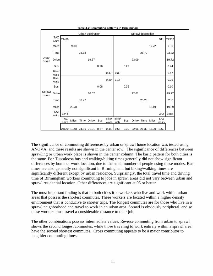
These results match most assumptions about the impacts of sprawl, but they do not take into account the location of employment. It may be that travel times and mode choice are influenced not just by home location but also by job locations. Job sprawl may have an important influence on commuting patterns, as workers commuting entirely within urban areas would likely have shorter commutes than those commuting to the city from sprawl areas. Testing this is possible using Part 3 of the CTPP. Home and Job Locations Part 3 of the CTPP lists the number of workers commuting between each pair of TAZs. The origin zone represents the workers home, while destinations are job locations. This allows both home and work locations to be classified as urban or sprawl, resulting in four possible combinations of commuting trips. Workers can commute from an urban home to an urban workplace, an urban home to a sprawl workplace, a sprawl home to an urban job, or a sprawl home to a sprawl job. It can be expected that there will be significant differences in commuting times and mileage between these four possibilities. Each of the commuting time variables were taken from Part 3, and mileage was calculated as discussed earlier. Because there are four possible commuting trip types, the average commuting values for each type was shown in a separate quadrant of the tables (Tables 4-2 and 4-3). Home locations in sprawl or urban areas are shown on the left side, with the destination of the commuting trip in urban or sprawl areas listed along the top.

Variable Urban Sprawl Urban Sprawl

Number of TAZs 646 62 204 59

Average Commute Miles 6.77 17.97* 4.47 16.61*

Average Commute Time 17.71 29.039* 16.16 29.734*Avrerage Drive Time 16.90 28.473* 15.97 28.895*

Average Bus Time 10.99 6.49 1.24 2.97

Average Bike/Walk Time 5.41 3.10 3.18 0.532**Average Number of Vehicles 1.25 2.19 1.51 2.16*

Percent Who Drive Alone 61.39 88.34 74.95 76.40

Percent who use transit 1.13 0.131** 0.15 0.46Percent who Bike/Walk 1.99 0.75 2.57 1.96

Percent leaving during Morning Rush 27.14 28.28 28.53 25.55

Population Density 947.56 66.832* 922.81 20.25*Worker Density 360.30 32.692* 391.84 8.599*

Household Density 392.52 24.46* 363.71 7.688*Housing Density 477.53 26.17* 405.61 7.969*

Percent White 42.40 91.11* 53.54 87.583*

Percent who are Homeowners 47.59 87.02* 52.88 87.909*Average Household Income ($) 38909.63 66725.24 39133.65 50026.61*

Percent Below Poverty 6.35 2.49 10.48 3.519*

Table 4-1. Commuting differences between sprawl and urban areas

* = significant differences at .01 or better; ** = significant at .05

11

The significance of commuting differences by urban or sprawl home location was tested using ANOVA, and these results are shown in the center row. The significance of differences between sprawling or urban work place is shown in the center column. The basic pattern for both cities is the same. For Tuscaloosa bus and walking/biking times generally did not show significant differences by home or work location, due to the small number of people using these modes. Bus times are also generally not significant in Birmingham, but biking/walking times are significantly different except by urban residence. Surprisingly, the total travel time and driving time of Birmingham workers commuting to jobs in sprawl areas did not vary between urban and sprawl residential location. Other differences are significant at 05 or better. The most important finding is that in both cities it is workers who live and work within urban areas that possess the shortest commutes. These workers are located within a higher density environment that is conducive to shorter trips. The longest commutes are for those who live in a sprawl neighborhood and travel to work in an urban area. Sprawl is obviously peripheral, and so these workers must travel a considerable distance to their job. The other combinations possess intermediate values. Reverse commuting from urban to sprawl shows the second longest commutes, while those traveling to work entirely within a sprawl area have the second shortest commutes. Cross commuting appears to be a major contributor to lengthier commuting times.

Urban destination Sprawl destinationTAZ pairs

21426 911 22337

Miles 9.00 17.72 9.36

Time 23.18 26.72 23.32

Urban origin Drive 19.57 23.09 19.72

Bus 0.76 0.29 0.74

Bike/ walk

0.47 0.32 0.47

Bike/ walk

0.20 1.17 0.29

Bus 0.08 0.35 0.10

Sprawl origin

Drive 30.52 22.61 29.77

Time 33.72 25.28 32.91

Miles 20.28 16.19 19.89

TAZ pairs

3244 342 3586

TAZ pairs Miles Time Drive Bus

Bike/ walk

Bike/ walk Bus Drive Time Miles

TAZ pairs

24670 10.48 24.56 21.01 0.67 0.44 0.55 0.30 22.96 26.33 17.30 1253

Table 4-2 Commuting patterns in Birmingham

12

The column totals along the bottom show averages by place of work, while the row totals along the right side show averages by place of residence. Because these values do not show workers who live in, or commute to, other counties, these totals will not necessarily be the same as that shown earlier for Part 1. Workers from sprawl homes have longer commutes than those from urban locations, but in both cases it is interesting that the longer commutes of workers traveling between sprawl and urban areas (in either direction) have increased the average commuting lengths. This raises the possibility that moving jobs to outlying locations would decrease commuting times for sprawl residents (but increase them for urban residents). As more workers move to sprawl homes, average metropolitan commuting lengths could therefore decrease.

Urban destination Sprawl destinationTAZ pairs

2933 78 3011

Miles 4.18 15.77 4.48

Time 14.99 23.34 15.21Urban origin

Drive 12.88 20.1213.07

Bus 0.10 ---- 0.10Bike/walk

0.61 ---- 0.60Bike/walk

0.47 0.47 0.47

Bus 0.12 ---- 0.11

Drive 24.51 10.9623.07

Sprawl origin Time 28.59 15.79 27.23

Miles 16.82 7.10 15.79TAZ pairs

481 57 538TAZ pairs Miles Time Drive Bus

Bike/walk

Bike/walk Bus Drive Time Miles

TAZ pairs

3414 5.96 16.91 14.52 0.10 0.59 0.20 0.00 16.26 20.15 12.11 135

Table 4-3 Commuting patterns in Tuscaloosa

13

Section 5 Conclusions and Recommendations

Generalizations about Sprawl and Commuting The relationships found between commuting and sprawl in Birmingham and Tuscaloosa provide empirical confirmation of widespread assumptions about sprawl, as well as showing the magnitude of the difference that sprawl makes. The discussion in this section supports the general body of existing work, as illustrated by citations taken from the literature. The major contribution of this research is to show how commuting patterns vary between (and within) sprawl and urban areas, and how it contributes to overall metropolitan commuting patterns. Using origin-destination data (Section 3 of this report) is particularly revealing of the importance of sprawl to commuting, and the interrelationships that exist between workplace and home locations. People who travel from sprawling areas to urban jobs have the longest commutes, while those who commute entirely within sprawl commute fewer minutes, though not as few as those who travel between urban homes and urban jobs. Cross commuting is clearly a contributor to longer average commute times. These results suggest that commuting patterns may be altered by the continuing decentralization of jobs and workers. If workers move to sprawling areas but continue to work in urban areas, metropolitan commuting times can be expected to greatly increase. However, if jobs follow the movement of population to sprawl areas, then metropolitan commuting time averages should decrease. The latter possibility has also been observed at the metropolitan level (Crane and Chatman 2004). Increasing sprawl could potentially result in commuting times within sprawl and older urban areas becoming more equal. It is clearly important to understand commuters’ workplace and residential histories to verify if this is in fact the case. It is also important to examine workers’ residential preferences, as this has been shown to affect commuting choices (Schwanen and Mokhtarian 2005). A person’s desire to live in a particular type of urban area may be reflected in mode choice, so that someone who lives in an urban area, but would rather live in suburbs, may rely on automobiles for trave l whether he or she has other choices or not. It has been suggested that “rather than trying to motivate suburbanites-at-heart to move to urban areas against their true preferences, simply make it easier for those who want to live in such areas anyway to do so” (Schwanen and Mokhtarian 2005, 97). Given that sprawl could result in reduced commuting times, the shift of jobs from urban areas to sprawl may be a better fit for many workers’ preferences and may provide the benefit of shorter, or at least constant, commuting times within the metropolitan area. Of the general original-destination, mode choice and commuting factors in this study, all but one follow the expected patters. The lack of differences between transit and biking/walking travel times is surprising, but is probably due to the small number of people using these modes in Alabama. This shows that the effects sprawl can be expected to take a range of manifestations

14

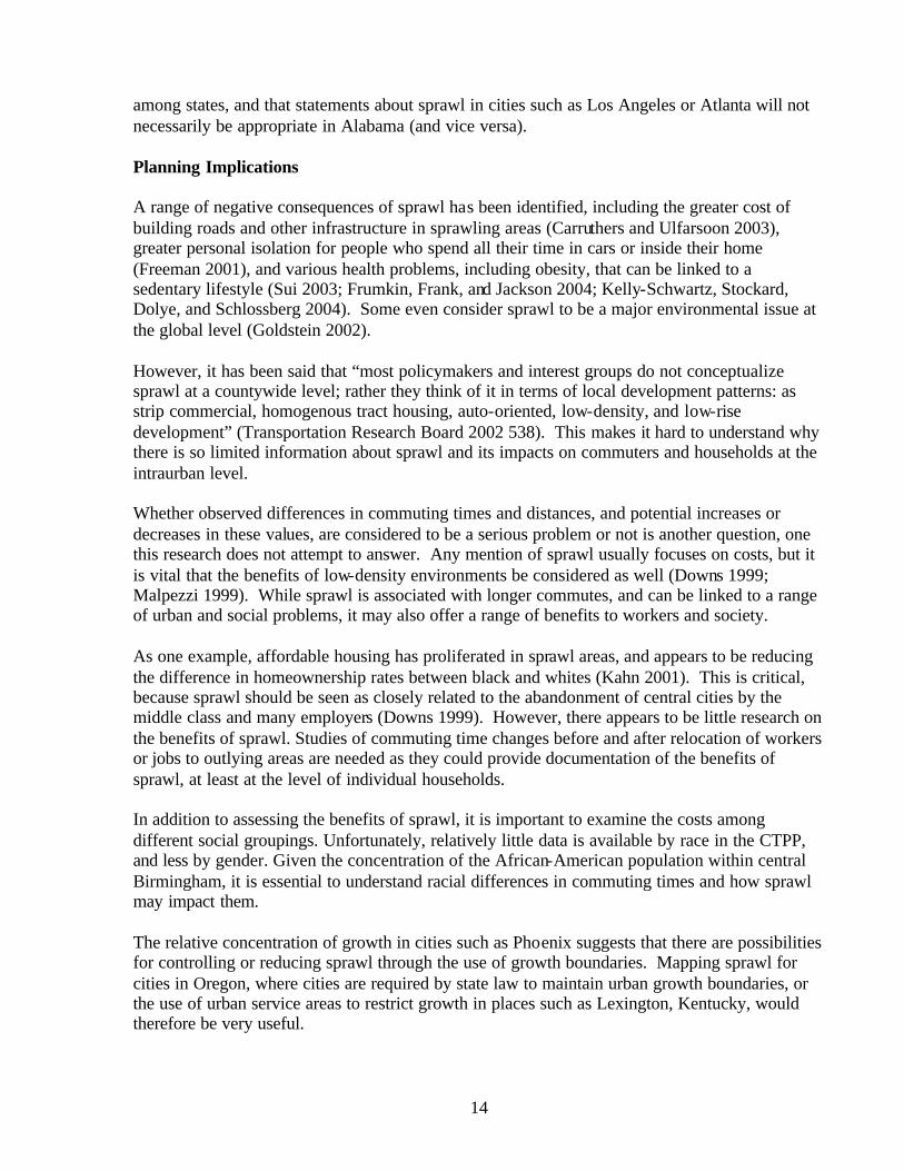
among states, and that statements about sprawl in cities such as Los Angeles or Atlanta will not necessarily be appropriate in Alabama (and vice versa). Planning Implications A range of negative consequences of sprawl has been identified, including the greater cost of building roads and other infrastructure in sprawling areas (Carruthers and Ulfarsoon 2003), greater personal isolation for people who spend all their time in cars or inside their home (Freeman 2001), and various health problems, including obesity, that can be linked to a sedentary lifestyle (Sui 2003; Frumkin, Frank, and Jackson 2004; Kelly-Schwartz, Stockard, Dolye, and Schlossberg 2004). Some even consider sprawl to be a major environmental issue at the global level (Goldstein 2002). However, it has been said that “most policymakers and interest groups do not conceptualize sprawl at a countywide level; rather they think of it in terms of local development patterns: as strip commercial, homogenous tract housing, auto-oriented, low-density, and low-rise development” (Transportation Research Board 2002 538). This makes it hard to understand why there is so limited information about sprawl and its impacts on commuters and households at the intraurban level. Whether observed differences in commuting times and distances, and potential increases or decreases in these values, are considered to be a serious problem or not is another question, one this research does not attempt to answer. Any mention of sprawl usually focuses on costs, but it is vital that the benefits of low-density environments be considered as well (Downs 1999; Malpezzi 1999). While sprawl is associated with longer commutes, and can be linked to a range of urban and social problems, it may also offer a range of benefits to workers and society. As one example, affordable housing has proliferated in sprawl areas, and appears to be reducing the difference in homeownership rates between black and whites (Kahn 2001). This is critical, because sprawl should be seen as closely related to the abandonment of central cities by the middle class and many employers (Downs 1999). However, there appears to be little research on the benefits of sprawl. Studies of commuting time changes before and after relocation of workers or jobs to outlying areas are needed as they could provide documentation of the benefits of sprawl, at least at the level of individual households. In addition to assessing the benefits of sprawl, it is important to examine the costs among different social groupings. Unfortunately, relatively little data is available by race in the CTPP, and less by gender. Given the concentration of the African-American population within central Birmingham, it is essential to understand racial differences in commuting times and how sprawl may impact them. The relative concentration of growth in cities such as Phoenix suggests that there are possibilities for controlling or reducing sprawl through the use of growth boundaries. Mapping sprawl for cities in Oregon, where cities are required by state law to maintain urban growth boundaries, or the use of urban service areas to restrict growth in places such as Lexington, Kentucky, would therefore be very useful.

15

The cities examined in this study show that sprawl can readily occupy small towns well removed from both urbanized and rural areas. Growth boundaries must therefore not just restrict new development within a particular urban area but also operate at a much larger spatial scale. Indeed, previous research (Weber and Maret 2003) has shown that rural sprawl is widespread in Alabama, indicating that growth boundaries originally limited to large cities are appropriate for smaller cities as well. Any effective anti-sprawl policy must operate by influencing land use development, not simply by encircling a problem area. This research presents an application of the CTPP, a data set in use by Alabama transportation planners as part of the standard metropolitan transport planning process. Using the CTPP to map sprawl could enable these planners to better understand the impacts of current growth pattens. Additionally, overlaying the sprawl database created with other digital data will allow integration with land use and natural resource planning, remote sensing data, historic preservation, economic development, site selection by both public agencies and private organizations, business management and logistics, allowing identification of the impact of sprawl on other facets of urban communities. Applicability to Other Areas The data used in this project is freely available from the U.S. Census Bureau and Bureau of Transportation Statistics, and the methodology developed in this project could be easily used in other Alabama metropolitan areas or those of other states. At the present time Part 3 has not been released on CD, although it is possible to download it from the Bureau of Transportation Statistics website (www.bts.gov). Although this was not a problem for Alabama metropolitan areas, downloading Part 3 for larger MSAs may be difficult as the resulting files are extremely large and may overwhelm some software systems. As noted above, the reliance on TAZs posed a number of problems. The 1990 CTPP software does not function with any operating system newer than Windows 95, so TAZs must be reconstructed from 1990 Blocks, while the population tables must be opened us ing a spreadsheet. Considerable editing is required to create the 1990s TAZs and interpolation must still be used to transfer population values to 2000 zones. As the shapefiles used in the 2000 CTPP software are proprietary, this lack of compatibility may reoccur for the 2010 CTPP. The use of Census Blocks or Tracts would remove these software difficulties, but these boundaries also change, and as data from the 2000 CTPP does exist for these zones, no relationships between sprawl and commuting could be established. Within Alabama TAZs have been defined not only for Tuscaloosa, Jefferson, and Shelby counties but also for other metropolitan areas. Expansion of this methodology to non-metropolitan counties would require the use of other Census units, such as Blocks or Tracts. These could be interpolated to raster surfaces to identify percentage change between 1990 and 2000, as has been done by Maret and Dakan (2003). But again, there would be no ability to integrate data from the 2000 CTPP. Recommendations for Further Work This research has shown that mapping sprawl at the intraurban level and assessing its relationship to travel behavior can be carried out relatively easily using GIS software and data

16

from the CTPP. Previous research and discussions of sprawl have not gone beyond discussing definitions and providing summary measures. This is therefore the first project to map sprawl within cities and to identify areas where growth patterns and traffic should be monitored. And because commuting is an inherently spatial act, there can be no meaningful discussion of the impact on sprawl without taking into account the actual location of sprawl within a metropolitan area, as well as relating it to the location of homes and workers. This research is also the first to accomplish this. Despite the significance and utility of this approach, it has several weaknesses and limitations. This approach simply identifies areas as sprawl or not sprawl, while a ranking or intensity value would be useful, so that the leve l of sprawl within a sprawling zone could be assessed. Making use of a ranking system for sprawl, as seen at the interurban level, would provide greater sensitivity to sprawl conditions and more precise understanding of its impacts on commuting patterns. As noted in Section 2, many measures of sprawl at the metropolitan level do rank individual metro areas by sprawl intensity, but these approaches are not readily transferable to the intraurban level. Rankings at the scale of TAZs or similar zones might instead be based on the magnitude of population density and growth. This research is based on discrete zones, which means that the results may vary according to the number, size, and boundaries of these zones. This is known as the Modifiable Areal Unit Problem, or MAUP (Openshaw 1996; Green and Flowerdew 1996). This problem results from the fact that the size and shape of zones, no matter how disaggregate, will influence observed averages and relationships. These problems exist not only for arbitrary zones such as city boundaries, which may have a weak relationship to the actual urbanized area (Lamb 1983), but for all zones. Studies should use zones that reflect the scale at which the phenomena of interest operates, such as using a watershed to model water pollution. Using raster cells to represent sprawl has been suggested (Galster, et al 2001), but there are possibilities for making use of zones that are more appropriate for commuting patterns (Sultana 2002; Horner and Murray 2002; Hasse and Lathrop 2003). Perhaps the most significant limitation of this methodology is that it is based only on density and population growth rate. While this allows a straightforward definition and mapping, it does not take into account street patterns, presence or absence of sidewalk, leapfrog development, strip commercial development, or other manifestations of sprawl that can influence commuting and other travel behavior. Expanding the definition to take into account factors other than density and growth rate would therefore be very useful. However, many of these possibilities would require data not available in the CTPP or Census data, such as land use mix, street characteristics, or housing unit level population data. One possibility for obtaining this data is from remote sensing sources, such as aerial photography or even satellite imagery (Ryznar and Wagner 2001; Stanilov 2002; Hasse and Lathrop 2003). This data can be integrated relatively easily with other GIS data, and may be an excellent choice for mapping and ana lyzing sprawl in Alabama. The possibility of using such remotely sensed data to measure transportation phenomena such as traffic counts by time of day or proximity to bus stations and availability of sidewalks also exists (Cowen and Jensen 1998) and should be examined.

17

Section 6

References Berman, Michael A. 1996. The transportation effects of neo-traditional development. Journal of

Planning Literature 10: 347-363. Boarnet, Marlon G., and Randall Crane. 2001. Travel by Design: the Influence of Urban Form

on Travel. Oxford: Oxford University Press. Carruthers, John I., and Gudmundur F. Ulfarsson. 2003. Urban sprawl and the cost of public

services. Environment and Planning B 30: 503-522. Chapman, Nancy, and Hollie Lund. 2004. Housing density and livability in Portland. In The

Portland Edge: Challenges and Successes in Growing Communities, edited by Connie P. Ozawa. Washington, DC: Island Press.

Cowen, David J., and John R. Jensen. 1998. Extraction and modeling of urban attributes using remote sensing technology. In People and Pixels: Linking Remote Sensing and Social Science, edited by Diana Liverman, Emilio F. Moran, Ronald R. Rindfuss, and Paul C. Stein. Washington, DC: National Academy Press.

Crane, Randall. 1996. On form versus function: will the New Urbanism reduce traffic, or increase it? Journal of Planning Education and Research 15: 117-126.

Crane, Randall, and Richard Crepeau. 1998. Does neighborhood design influence travel?: A behavioral analysis of travel diary and GIS data. Transportation Research D 3: 225-238.

Crane, Randall, and Daniel G. Chatman. 2004. Traffic and sprawl: evidence from US commuting 1985-1987. In Urban Sprawl in Western Europe and the United States, edited by Harry W. Richardson and Chang-Hee Christine Bae. Aldershot: Ashgate.

Dakan, William, and Isabelle Maret. 2002. Delineating Urban and Non-Urban Sprawl: A GIS Approach in the Southeastern U.S. Paper presented at the Annual Meeting of the Southeastern Division of the Association of American Geographers, Richmond, Virginia, November 23 – 26.

Downs, Anthony. 1999. Some realities about sprawl and urban decline. Housing Policy Debate 10: 955-974.

El Nasser, Haya, and Paul Overberg. 2001. A Comprehensive Look at Sprawl in America. www.usatoday.com/news/sprawl/main/htm. Retrieved 28 September 2004.

Ewing, R., R. Pendall, and D. Chen. 2004. Measuring Sprawl and Its Impact: The Character and Consequences of Metropolitan Expansion. http://www.smartgrowthamerica.org. Retrieved November 26, 2004.

Frank, L., and G. Pivo. 1994. Relationships between Land Use and Travel Behavior in the Puget Sound Region. Seattle: Washington State Transportation Center.

Freeman, Lance. 2001. The effects of sprawl on neighborhood social ties. Journal of the American Planning Association 67: 69-77.

Friedman, Bruce, Stephen P. Gordon, and John B. Peers. 1994. Effect of neotraditional neighborhood design on travel characteristics. Transportation Research Record 1466: 63-70.

Frumkin, Howard, Lawrence Frank, and Richard Jackson. 2004. Urban Sprawl and Public Health: Designing, Planning, and Building for Healthy Communities. Washington, DC: Island Press.

18

Galster, G., R. Hanson, M.R. Ratcliffe, H. Wolman, S. Coleman, and J. Freihage. 2001. Wrestling Sprawl to the Ground: Defining and Measuring an Elusive Concept. Housing Policy Debate 12: 681-717.

Gillham, O. 2002. The Limitless City: A Primer on the Urban Sprawl Debate. Island Press, Washington DC.

Gober, Patricia, and Elizabeth K. Burns. 2002. The size and shape of Phoenix’s urban fringe. Journal of Planning Education and Research 21: 379-390.

Goldstein, Natalie. 2002. Earth Almanac: An Annual Geophysical Review of the State of the Planet, Second Edition. Westport, CT: Oryx Press.

Gordon, P., A. Kumar, and H.W. Richardson. 1989a. The influence of metropolitan spatial structure on commuting time. Journal of Urban Economics 26: 138-151.

Gordon, P., A. Kumar, and H.W. Richardson. 1989b. Congestion, changing metropolitan structure, and city size in the United States. International Regional Science Review 12: 45-56.

Gordon, P., H.W. Richardson, and Myung-Jin Jun. 1991. The commuting paradox: evidence from the top twenty. Journal of the American Planning Association 57: 416-420.

Green, M., and R. Flowerdew. 1996. New evidence on the modifiable unit problem. In Spatial Analysis: Modelling in a GIS Environment, edited by P. Longley and M. Batty. New York: John Wiley and Sons.

Gutfreund, Owen D. 2004. Twentieth-Century Sprawl: Highways and the Shaping of the American Landscape. Oxford: Oxford University Press.

Hamin, Elisabeth M. 2003. Mojave Lands: Interpretive Planning and the National Preserve. Baltimore: Johns Hopkins Press.

Handy, Susan. 1996. Methodologies for exploring the link between urban form and travel behavior. Transportation Research D 1: 151-165.

Hart, John Fraser. 1991. The perimetropolitan bow wave. Geographical Review 81: 37-51. Hasse, John, and Richard G. Lathrop. 2003. A housing-unit- level approach to characterizing

residential sprawl. Photogrammetric Engineering and Remote Sensing 69: 1021-1030. Horner, Mark W., and Alan T. Murray. 2002. Excess commuting and the modifiable areal unit

problem. Urban Studies 39: 131-139. Johnson, M. P. 2001. Environmental impacts of urban sprawl: a survey of the literature and

proposed research agenda. Environment and Planning A 33: 717-735. Kahn, Matthew E. 2001. Does sprawl reduce the black/white housing consumption gap?

Housing Policy Debate 12: 77-86. Kelly-Schwartz, Alexia C., Jean Stockard, Scott Doyle, and Marc Schlossberg. 2004. Is sprawl

unhealthy? A multilevel analysis of the relationship of metropolitan sprawl to the health of individuals. Journal of Planning Education and Research 24: 184-196.

Lamb, Richard F. 1983. The extent and form of exurban sprawl. Growth and Change 14: 40-47.

Lang, Robert E. 2003. Open spaces, bounded places: does the American West’s arid landscape yield dense metropolitan growth? Housing Policy Debate 13: 755-778.

Levinson, D.M., and A Kumar. 1997. Density and the journey to work. Growth and Change 28: 147-172.

Levinson, D.M., and A. Kumar. 1994. The rational locator: why travel times have remained stable. Journal of the American Planning Association 60: 319-332.

Malpezzi, S. 1999. Estimates of the measurements and determinants of Urban Sprawl in US Metropolitan Areas. Madison: Center for Urban Land Economics, University of Wisconsin.

19

Openshaw, Stan. 1996. Developing GIS-relevant zone-based spatial analysis methods. In Spatial Analysis: Modelling in a GIS Environment, edited by P. Longley and M. Batty. New York: John Wiley and Sons.

Remington, W. Craig, ed. 2002. Atlas of Alabama Counties, Fourth Edition. Tuscaloosa: University of Alabama Department of Geography Cartographic Research Laboratory.

Ryznar, Rhonda M., and Thomas W. Wagner. 2001. Using remotely sensed imagery to detect urban change: viewing Detroit from space. Journal of the American Planning Association 67: 327-336.

Schwanen, Tim, and Patricia Mokhtarian. 2005. What affects commute mode choice: neighborhood physical structure or preferences toward neighborhoods? Journal of Transport Geography 13: 83-99.

Stanilov, Kiril. 2002. Postwar trends, land-cover changes, and patterns of suburban development: the case of Greater Seattle. Environment and Planning B 29: 173-195.

Sui, Daniel Z. 2003. Musings on the fat city: are obesity and urban forms linked? Urban Geography 24: 75-84.

Sultana, Selima. 2002. Job/Housing Imbalance and Commuting Time in the Atlanta Metropolitan area: Exploration of Causes of Longer Commuting time. Urban Geography 23: 728-749.

Sultana, Selima, and P. Chaney. 2003. Impact of Urban Sprawl on Trave l Behaviors and Local Watersheds in the Auburn-Opelika Metropolitan Area: A Case Study on a Small MSA. Papers and Proceedings of the Applied Geography Conference, Vol. 26.

Transportation Research Board. 2002. Costs of Sprawl – 2000. TCRP Report 74. Washington, DC: National Academy Press.

Tsai, Yu-Hsin. 2005. Quantifying urban form: compactness versus ‘sprawl’. Urban Studies 42: 141-161.

Weber, Joe, and Isabelle Maret. 2003. Urban Sprawl and Access to Public Transportation. Paper presented at the 42nd Annual Southern Regional Science Association Meeting, Louisville, KY, April 10-12.

Wolch, Jennifer, Manuel Pastor Jr., and Peter Dreier, eds. 2004. Up Against the Sprawl: Public Policy and the Making of Southern California. Minneapolis: University of Minnesota Press.

Wolman, Harold, George Galster, Royce Hanson, Michael Ratcliffe, Kimberly Furdell, and Andrea Sarzynski. 2005. The fundamental challenge in measuring sprawl: which land should be considered? Professional Geographer 57: 94-105.