The Impact of Organizational Structure and Lending Technology

on Banking Competition

Hans Degryse CentER - Tilburg University, TILEC, KU Leuven and CESifo

Department of Finance

PO Box 90153, NL 5000 LE Tilburg, The Netherlands Telephone: +31 13 4663188, Fax: +31 13 4662875

E-mail: h.degryse@uvt.nl

Luc Laeven∗∗∗∗

International Monetary Fund, CEPR and ECGI

Research Department 700 19th Street NW, Washington DC, 20431, USA

Telephone: +1 202 623 9020, Fax: +1 202 623 4740 E-mail: llaeven@imf.org

Steven Ongena CentER - Tilburg University and CEPR

Department of Finance

PO Box 90153, NL 5000 LE Tilburg, The Netherlands Telephone: +31 13 4662417, Fax: +31 13 4662875

E-mail: steven.ongena@uvt.nl

First Draft: February 21st, 2006 This Draft: February 16th, 2007

∗ Corresponding author. We are grateful to Klaus Adam, Lamont Black, Elena Carletti, Giovanni Dell’Ariccia, Valeriya Dinger, Don Fraser, Robert Hauswald, Jan Krahnen, Jose Liberti, Fabio Panetta, Efrat Tolkowsky, as well as seminar participants at the 2006 European Finance Association Meetings (Zurich), 2006 Changing Geography of Banking Conference (Ancona), 2006 CEPR European Summer Symposium on Financial Markets (Gerzensee), 2006 Konstanz Seminar on Monetary Theory and Policy (Island of Reichenau), the joint ECB-CFS-Bundesbank Lunch Seminar, Norges Bank, the University of Ghent, and Maastricht University for many valuable comments. Degryse gratefully acknowledges financial support from FWO-Flanders, NWO-The Netherlands, and the Research Council of the University of Leuven. Degryse holds the TILEC-AFM Chair on Financial Regulation. We would like to thank Thomas Provoost for data assistance. The paper was partly written while Laeven was at the World Bank. This paper’s findings, interpretations, and conclusions are entirely those of the authors and do not necessarily represent the views of the International Monetary Fund, its Executive Directors, or the countries they represent.

The Impact of Organizational Structure and Lending Technology

on Banking Competition

Abstract: Recent theoretical models argue that a bank’s organizational structure reflects its

lending technology. A hierarchically organized bank will employ mainly hard information,

whereas a decentralized bank will rely more on soft information. We investigate theoretically

and empirically how bank organization shapes banking competition. Our theoretical model

illustrates how a lending bank’s geographical reach and loan pricing strategy is determined

not only by its own organizational structure but also by organizational choices made by its

rivals. We take our model to the data by estimating the impact of the lending and rival

banks’ organization on the geographical reach and loan pricing of a singular, large bank in

Belgium. We employ detailed contract information from more than 15,000 bank loans

granted to small firms, comprising the entire loan portfolio of this large bank, and

information on the organizational structure of all rival banks located in the vicinity of the

borrower. We find that the organizational structures of both the rival banks and the lending

bank matter for branch reach and loan pricing. The geographical footprint of the lending

bank is smaller when rival banks are large and hierarchically organized. Such rival banks

may rely more on hard information. Geographical reach increases when rival banks have

inferior communication technology, have a wider span of organization, and are further

removed from a decision unit with lending authority. Rival banks’ size and the number of

layers to a decision unit also soften spatial pricing. We conclude that the organizational

structure and technology of rival banks in the vicinity influence local banking competition.

Keywords: banking sector, competition, hierarchies, authority, technology.

JEL: G21, L11, L14.

Introduction

The allocation of control within organizations shapes agents’ incentives (see e.g.

Grossman and Hart (1986), Hart (1995), and Hart and Moore (2005)). Organizational

theories of the firm have only recently been applied to the banking industry. Stein (2002),

for example, shows that a centralized hierarchical bank offers greater incentives to employ

information that is easy to communicate and store within an organization – i.e., “hard”

information – whereas, in contrast, a decentralized bank provides an environment

advantageous to “soft” information.1 And Petersen and Rajan (2002) document that banks

that rely more on hard information communicate in more impersonal ways with their

borrowers.

Hence, the bank’s mode of organization influences the lending technology employed.

Aghion and Tirole (1997) show that the amount of communication in an organization

depends on the allocation of authority, suggesting that the information generated at a bank

branch depends on the extent to which authority has been delegated to this branch. For a

sample of large U.S. firms, Rajan and Wulf (2006) find that the number of positions

reporting to the CEO and the level of authority delegated to division managers have both

increased significantly in recent years.

We present a stylized model that embeds these drivers to explain geographical reach and

spatial pricing in lending. We build a spatial discrimination model, starting from a

Hotelling (1929) – framework, to show how a bank’s own and its rivals’ organizational

choices may shape banking competition. In particular, we incorporate in our framework

1 In addition to these principal-agent theories of the firm, there also exists a large literature on transaction costs theories. See, for example, Williamson (1967, 1975). In Arrow (1975) the rationale for vertical integration of firms is to remove informational asymmetries within the firm. Earlier theoretical work on the communication and processing of information within organizations includes Cremer (1980), Radner (1993) and Bolton and Dewatripont (1994). None of these studies consider managers’ incentives and agency problems.

2

how bank hierarchy influences distance-related transportation costs incurred by either

borrowers or banks, and how differences in bank’s technology affect branch reach. Our

model shows that when rival banks are more hierarchically layered, the bank’s own

geographical reach shrinks and spatial pricing softens. The underlying rationale is simply

that hierarchically organized rival banks employ more hard information in reaching their

loan decisions, reducing either the borrowers’ or their own transportation costs. Also,

differences in technology and organizational swiftness between the lending bank and its

rivals affect their geographical reach.

To test the key hypotheses emanating from our theory, we combine two unique data sets

that contain detailed loan contract, firm, branch and bank information, including

information about the organizational form of each bank. The first data set contains detailed

contract information, including firm and lending branch location, for more than 15,000

loans to (mainly) small businesses. The second data set includes comprehensive

information on all 145 banks operating in Belgium, detailing for 7,477 branches of these

banks: (1) physical location, (2) organizational position and status, and (3) communication

technology.

Consequently, the combination of the two datasets encompasses information on the

complete set of loans granted to small and medium-sized business borrowers by a single

large bank in Belgium, the lending branch’s position in the lending bank’s organization,

and the organization structure of all the branches of rival banks in the vicinity of the

borrower’s location, resulting in around 250,000 borrower – rival bank branch

combinations.

We exploit the heterogeneity in banks’ organizational structure to identify the impact

lending technology has on the geographical reach and spatial pricing at bank branches. We

3

construct two types of empirical proxies for organizational complexity. The first are bank-

specific and identify heterogeneity in rival banks, i.e., bank size and the degree of

organizational hierarchy. The second are branch-specific and incorporate both lending

branch and rival branch characteristics, i.e., span of organization and the number of levels

to a decision unit (telex) to capture the degree to which lending authority has been

delegated. Finally, we use the presence of a fax to capture the lending technology at each

branch.

We find that the banks’ organizational form matters for both branch reach and the degree

of spatial pricing. The presence of a large and more hierarchically organized rivals in the

vicinity shrinks the geographical reach of the lending branch, as lending decisions of large

banks possibly become more driven by hard information. Also, when branches of rival

banks exhibit a greater organizational span of control (relative to the lending branch) and

are further removed from a unit with lending authority (as captured by a greater number of

layers to telex), the geographical reach of the lending branch increases. The presence of

rival banks that are large, have a large span of organization, and have many layers to the

telex attenuates spatial pricing. Hence, organizational form of the lending branch, and size

and hierarchy of rival banks in the vicinity of a borrower, determines both geographical

reach and loan pricing.

Empirical work analyzing how the nature of a bank’s organization affects the way it does

business typically suffers from a lack of data on the organizational form of the banks.

Existing work typically uses the size of the bank as a proxy for organizational complexity.

Berger, Miller, Petersen, Rajan and Stein (2005), for example, show that small banks are

indeed better able to collect and act on soft information. They also report that large banks

lend at greater distance and in a more impersonal way than small banks do. Liberti (2004)

examines how a change in the organizational form within a large bank affects incentives.

4

He finds that the reliance on soft information is higher under decentralized than centralized

structures. Liberti (2005) analyzes how information flows within the organization both

across layers (vertically) and horizontally (number of branch officers reporting to a

supervisor). He demonstrates that loan applications that need to pass more organizational

layers for approval are based more on hard information. This internal ‘hardening’ of the

information requirements however is mitigated when direct contact between the bottom and

top organizational layer is possible. Also loans granted directly by the branch, as well as

branches with ‘leaner’ horizontal organization can employ more soft information.

We contribute to this empirical literature by constructing and analyzing a novel dataset

that contains information on the hierarchical structure of all banks in Belgium, and by

highlighting the role of rival banks’ organizational form.

We organize the rest of the paper as follows. Section I introduces a stylized model of

banking competition. Section II introduces the data and variables employed in the

empirical analysis. Section III presents our empirical results. Section IV concludes.

5

I. Theory

Recent theoretical and empirical work highlights the importance of geographical distance

for the mode of interaction between banks and firms and for pricing of bank loans. In this

section we model and explore the impact of bank heterogeneity on bank branch reach and

loan pricing. We develop a stylized model in which firms can borrow at branches from

different banks. Banks themselves differ in their organizational form creating a different

specialization in dealing with hard or soft information. Our theoretical model takes the

organizational form of the bank and its branch as exogenously given. We then formulate

testable hypotheses about the impact of bank type on branch reach and loan pricing. In

particular, our model identifies how distance-related costs that are bank (and branch)

specific further increase the economic relevancy of geography and spatial pricing.

A. Literature

Our main point of departure is that lending conditions not only depend on the distance

between the borrower and the lender and the distance between the borrower and the closest

competing bank, but also on the characteristics of the banks involved. Our stylized

framework finds its inspiration in location differentiation models following Hotelling

(1929) (see Armstrong (2005) for a review). In these models, customers, in casu

borrowers, are typically assumed to incur identical (per unit of distance) transportation

costs when visiting a firm, i.e. a bank branch. An alternative, but for our purposes

strikingly similar, interpretation is developed in Sussman and Zeira (1995). They model

spatial pricing based on distance-related monitoring costs faced by the banks. In their

model the banks also face identical per unit of distance monitoring costs. While we will

formally derive our hypotheses placing the (differential) transportation costs with the

6

borrower, as is done in most models, we also acknowledge the equivalent interpretation in

which, as said, it is the lenders that face the distance-related monitoring costs.

Why would borrower or lender transportation costs depend on the type or organizational

form of banks involved? One straightforward explanation consists in the number of visits

the borrower has to make to the bank branch to obtain and service a loan (or the number of

visits the lender makes to screen and monitor the borrower). For example, if a borrower

knows her loan officer at the branch will insist on three face-to-face visits before granting

the loan (say one visit to file the loan application, one visit to negotiate the loan conditions,

and one visit to sign the final loan contract), her expected transportation costs will be three

times the costs visiting a one-stop bank branch were loan applications are approved on the

spot (or by mail afterwards). Alternatively, the borrower may know that loan officers from

one bank show up three times a year to check on their borrowers’ business, while another

bank may have a hands-off approach (entailing no monitoring). In both cases borrower and

bank ex ante know how many screening and/or monitoring visits are required to fully

bridge their informational asymmetries.

Recent theoretical work explains why loan officers working for different banks may

handle loan applications differently, causing the number of required visits to vary. Stein

(2002), for example, models the collection and transfer of information within hierarchical

versus decentralized financial institutions. Stein shows that centralization motivates loan

officers located in the branches to compile and transfer hard information (e.g., accounting

numbers) to support their demand for internal capital. Decentralization of decision-making

on the other hand provides loan officers incentives to collect and rely more on soft

information (e.g., impressions of borrower character), information that is by nature more

difficult to obtain and to transfer in an internal funding request.

7

If loan officers rely mostly on hard information, face-to-face contact with the borrower

becomes less important and more impersonal ways of communicating (such as telephone,

fax, or email) will gain ground (Petersen and Rajan (2002)).2 The number of personal visits

that is necessary to arrive at a loan decision or to monitor the borrower will become

smaller. On the other hand, when more soft information is employed, loan officers may

want to meet the applicant or visit her professional premises at least a few times to screen

and monitor the loan application. As a result, distance related costs per loan in the latter

“soft” case will be higher than in the former “hard” case.

Our stylized framework assumes that when the transportation costs are incurred, bank

officers perfectly solve the asymmetric information problem. We therefore assume that

loans are repaid with probability one (as long as the probability of repayment is identical

across borrowers and banks, qualitatively the same results hold). Hauswald and Marquez

(2006), on the other hand, specify a model where the quality of information decreases with

distance and informational problems linger. In particular, in their model the informational

signal the bank receives from close borrowers is more precise than the signal from far

borrowers. As a consequence the winner’s curse problem exacerbates when the bank

engages a borrower close to the rival bank. Banks also decide on the level of information

acquisition in Hauswald and Marquez (2006). More information acquisition aggravates the

winner’s curse problem and increases (in absolute value) the association between distance

and the loan rate. However their model only deals with symmetric equilibria in which

banks invest an equal amount in information acquisition. As a result their “transportation

2 Petersen and Rajan (2002) show that in the case of the US, where credit scoring of small business borrowers has become common practice among banks, the distance between small firms and their lenders has been increasing and banks and firms started to communicate in more impersonal ways. In Belgium, however, credit scoring of small firms was virtually non-existent during our sample period (1995-1997), and hence distance still plays an important role for the firms in our sample.

8

costs” are identical, while we, in admittedly a much more stylized setup, allow for

differences in transportation costs.

B. Model

We now introduce the different transportation costs into the stylized framework to explore

its impact on bank branch reach and loan pricing. As discussed previously, different

transportation costs capture the differences in the number of visits borrowers or lenders

make, possibly as a result of the varying bank organizational structure influencing the

banks’ usage of hard and soft information. We analyze branch reach and loan pricing when

firms differ in terms of location, but banks’ organizational form implies differences in their

usage of hard and soft information.

1. Non-Linear Transportation Costs

Formally we assume there are two bank branches from two different banks, denoted A and

B, at opposite ends of a line of length L . Borrowers are uniformly distributed across the

line with density one. We assume that a borrower located at x faces non-linear

transportation costs αxtA and α)( xLtB − in visiting branch A and B respectively. The slope

parameters At and Bt are associated with the impact of distance to reach branch A and B,

respectively. Bhaskar and To (2004) derive the solution to this non-linear transportation

problem for the case where the slope parameters are equal, i.e., BA tt = . We study the more

general case BA tt ≠ , with the difference capturing (as already indicated) the fact that

branches may have different screening and monitoring technologies and may rely on a

different mix of hard and soft information.

In taking a loan at branch A, a borrower located at x incurs a cost:

αxtr AAx + ,

9

with Axr the (net of repayment of the initial investment) loan rate charged by branch A to a

borrower located at x . Similarly, borrowing from branch B implies a cost:

α)( xLtr BBx −+ .

A borrower located at x is indifferent between borrowing from A or B when:

αα )( xLtrxtr BBxAAx −+=+ .

We assume that borrowers cannot arbitrage among each other in order to benefit from

lower loan rates and that their willingness to pay is high enough to guarantee they take a

loan in equilibrium. We further assume that both branches have information about the

borrower’s location before pricing the loan and that both branches have information about

the transportation costs the borrowers face to visit either bank, such that branches perfectly

price discriminate based upon borrower’s location and the difference in transportation costs

to visit either bank branch (as in Thisse and Vives (1988)).

For a borrower close by, i.e., 0=x , branch A enjoys some local market power, as from

the borrower’s perspective branch B’s best loan rate offer is its marginal cost of obtaining

funds plus her own transportation costs to B. We normalize marginal costs for both

branches to zero, and assume the same willingness to pay for obtaining a loan at both

branches. We will relax this assumption to deal with (other) issues of organizational span

and internal swiftness in the next subsection. For zero marginal costs at both branches, it is

clear then that branch A can charge αLtr BA =0 . That is, branch A can appropriate the

borrower’s transportation cost to branch B. Similarly, for Lx = , branch B charges

αLtr ABL = and appropriates that borrower’s transportation cost to branch A.

Let y be the borrower that receives a perfectly competitive loan rate 0== ByAy rr , as:

10

αα )( yLtyt BA −= .

All borrowers x to the left of y ( Lyx ≤≤≤0 ) are being serviced by branch A at a loan

rate:

( ) ααxtxLtr ABAx −−= .

That is, branch A charges a borrower at x the savings in transportation costs it makes

from borrowing at A rather than B.

Branch A’s total borrower portfolio y or geographical reach is determined by 0=Ayr ,

such that:

α/1

=

− A

B

t

t

yL

y, or

α

α

/1

/1

1

+

=

A

B

A

B

t

t

t

tL

y .

For changes in x , the change in interest rate equals:

( ) 11 −−−−−= αα

αα xtxLtdx

drAB

Ax .

Hence, our stylized model yields two testable hypotheses: (1) the geographical reach y of

branch A depends on At and on Bt , and (2) the slope of spatial pricing dx

drAx is negative and

depends on At and Bt . While branch A’s reach increases in the rival’s transportation costs

Bt but decreases in the own transportation cost At , the degree of spatial pricing measured

by the absolute value of the slope increases in At and Bt .3

3 In our empirical investigation, we assume logarithmic transportation costs. This yields similar predictions.

11

2. Linear Transportation Costs

To illustrate the main intuition in our model we set 1=L and 1=α . In this case, the

borrower receiving the perfect competitive loan rate 0== ByAy rr is located at:

BA

B

tt

ty

+= .

All borrowers “to the left” of y ( 10 ≤≤≤ yx ) are served by branch A at a loan rate:

( ) xtttxtxtr BABABAx )(1 +−=−−= .

The other borrowers ( 10 ≤≤≤ xy ) are served by branch B at loan rate:

( ) xtttxtxtr BABBABx )(1 ++−=−−= .

Figure 1 displays the resulting linear loan rate schedules for borrowers of both A and B.

The figure further highlights the two testable implications of our model. First, market

shares y and y−1 of branches A and B equal BA

B

tt

t

+ and

BA

A

tt

t

+, respectively. Hence a

decrease in transportation cost to the rival branch reduces the own market share. The

opposite result holds for the own transportation cost (notice that a uniform distribution of

borrowers further implies that market share equals branch size; since the length of the line

is normalized to one, geographical reach equals in this case branch size). Second, the rate

at which both branches discriminate in distance (i.e., the absolute value of the slopes of

both schedules) equals BA tt + , hence increases in both At and Bt .

3. Differential Marginal Costs

Assume, for example, that the marginal cost for branch B equals 0>µ , while the

marginal cost for branch A equals zero. With appropriate modifications, µ could also

reflect the differential repayment probabilities to the two branches, or differences in

12

willingness-to-pay for loans from a specific branch. When branch B uses inferior

technology, for example, or when its international organization is such that it does not have

the authority or capacity to make quick decisions on loan approvals, its µ would be

positive. In this setting, branch A now appropriates the close borrower’s transportation cost

to branch B plus the marginal cost differential. Hence, for 0=x , branch A charges

µ+= BA tr 0 . Branch B can only charge AB tr =0 to the close borrower. Let y again be the

borrower that receives the most competitive loan rate from both A and B, i.e. 0=Ayr and

µ=Byr , then µ+−= )1( ytyt BA and:

BA

B

tt

ty

+

+=

µ.

All borrowers “to the left” of y ( 10 ≤≤≤ yx ) are served by branch A at a loan rate:

( ) xtttxtxtr BABABAx )(1 +−+=−+−= µµ .

The other borrowers ( 10 ≤≤≤ xy ) are served by branch B at loan rate:

( ) xtttxtxtr BABBABx )(1 ++−=−−= .

Consequently the market reach (and share) of branch A increases in the marginal cost

differential µ . Put differently in terms of technology differences, branch reach increases in

the technology differential between the own branch and the rival branch. However the rate

at which both branches discriminate remains unaltered and equal to BA tt + .

To conclude, differential transportation and marginal costs determine branch geographical

reach and loan pricing. In particular, relatively lower transportation costs to a rival bank

branch limits the geographical reach of the own branch and the slope of spatial pricing,

while higher marginal costs (or inferior technology) at a rival branch extends the own reach

13

(Appendix 1 analyzes how borrower-specific transportation costs stemming from

information availability can further enrich this picture). We now turn to testing these

theoretical predictions.

II. Data and Variables

A. Data

The dataset we analyze consists of 15,044 loans made to independents or single-person

businesses, and small-, medium-, and large-sized firms by an important Belgian bank that

operates throughout Belgium. Degryse and Van Cayseele (2000) first employed the bank-

firm relationships data set, while Degryse and Ongena (2005) added distance variables and

showed that both distance to lender and distance to closest competitor play a role in loan

pricing.

The sample encompasses all existing small and medium enterprise loans granted by this

Belgian bank as of August 10, 1997 that were initiated or repriced after January 1, 1995.

The bank is one out a few truly national and general-purpose banks operating in Belgium in

1997. It lends to firms located in most postal zones, and is active in 49 different industries.

Around 83% of the firms in its portfolio are single-person businesses and most borrowers

obtain just one (relatively small) loan from this bank. As of December 31st, 1994, we

identify 7,477 branches, operated by 145 different banks and located in 837 different postal

zones.

Each postal zone carries a postal code between 1,000 and 9,999. The first digit in the code

indicates a geographical region, which we call “postal area” and which in most cases

coincides with one of the ten Provinces in Belgium. A postal zone covers on average 26 sq

km, and contains on average approximately six bank branches. A postal area covers 3,359

sq km, on average. Not surprisingly, borrowers are often located in more densely banked

14

areas, with on average more than 17 bank branches per postal zone, resulting in around

250,000 possible borrower – competing bank branch pairs.

Table 1 provides summary statistics for the 15,044 contracts of our variables, broken

down into eight sets of characteristics: (1) dependent variables; the transportation cost

drivers of interest: (2) bank organization and technology, (3) bank and market type, and (4)

geographical distance; and the control variables: (5) postal zone variables (6) relationship

characteristics, (7) loan contract characteristics, (8) loan purpose, (9) firm characteristics,

and (10) interest rate variables.

B. Dependent Variables

Our theoretical model suggests employing two different dependent variables. The first is

Branch Reach. We distinguish Quartile Reach, computed as the log of one plus the

traveling time of the branch’s quartile most remote borrower and the branch itself, in

minutes, and Maximum Reach, representing the log of one plus the maximum distance

between the most remote borrower and the branch.4 The mean across all branches for

Quartile (Maximum) Reach is 2.60 (3.52), translating into approximately 14 (40) minutes

traveling time to the remote borrower (see Table 1). We will also check the robustness of

our findings using the Number of Loans as measures of branch size (as branch reach and

size are equivalent in our theoretical framework).

The second dependent variable is the Loan Rate, the interest rate on the loan until the next

revision. For fixed interest rate loans, this is the yield to maturity of the loan. For variable

interest rate loans, this is the interest rate until the date at which the interest rate will be

revised as stipulated in the contract. The average interest rate on a loan in our sample is

8.12% or 812 basis points (we employ basis points throughout the paper). The loan rate

4 Degryse and Ongena (2005) provide more details on computational issues related to our distance-variables as well as other minor sample selection issues.

15

varies widely not only nationally (the standard deviation is 236 basis points), but also at the

branch level (the average standard deviation at the branch level is still 217 basis points).

We will also check the robustness of our findings using the natural logarithm of Loan Size

as an independent variable (we will multiply this variable times 1,000 to get easily readable

coefficients). The median loan size is around 300,000 Belgian Francs (7,500 US Dollar).5

C. Bank Organization and Technology

Our theoretical model suggests that the mode of organization and the lending technology

employed by the lending branch and the closest competitor matters for branch reach and the

degree of spatial pricing. The Belgian financial landscape shows substantial heterogeneity

in rival banks. In addition to other large banks, a number of smaller (savings) banks are

also present. To address the impact of organizational structure and technology, we

combine the loan information data set employed by Degryse and Ongena (2005) with a new

data set on the type and organizational structure of all bank branches in Belgium.

We introduce two variables that measure a bank’s specific internal organization. First, we

start by constructing a variable Large Bank, which measures the size of the geographically

closest bank, in terms of total assets, relative to the largest bank.6 Large Bank ranges

between zero and one, and equals one when the closest competitor is the largest bank. We

obtain data on the total assets of all banks in Belgium from the Documenten en Aspecten

(Documents and Aspects) published by the Belgische Vereniging van Banken (Belgian

Bankers Association). Summary statistics reported in Table 1 show that Large Bank is on

average 0.62.

5 40 Belgian Francs (BEF) are approximately equal to 1 US$ during the sample period.

6 As for the other relevant variables we actually average across the 25% geographically closest competitors.

16

Second, we measure the Hierarchy of the closest competitor at the bank level (Hierarchy

Bank). Stein (2002), for example, shows that a centralized hierarchical bank offers an

environment advantageous to hard information. For each branch in the bank we follow the

‘chain of command’ all the way up to the top branch that has no reporting duty (to a higher

level) and count the layers traveled. The levels per branch counted in this way range

between zero and five. We can construct this variable on the basis of information from the

1994 annual report Bankkantoren in België (Bank Branches in Belgium) published by the

Belgische Vereniging van Banken (Belgian Bankers Association). This document lists to

which branch higher up in the hierarchy of the bank each of the 7,477 branches reports.

We then (1) average the counted levels across the branches of each bank, (2) take the

value of this measure for the closest competitor, and (3) scale by the maximum across

banks (which is around four). This constitutes our measure of hierarchy for each bank. By

construction Hierarchy Bank ranges between zero and one, and does not exhibit

heterogeneity between branches of the same bank. The average is 0.366 indicating that the

competing bank branch has around 1.5 levels of organizational layers above it.

Importantly, Table 2 indicates that bank size and hierarchy and are only weakly correlated,

with a correlation coefficient of 0.375.

While Large Bank and Hierarchy Bank only take information from competing banks into

account (as such do not exhibit heterogeneity for the branches of the lending bank), we next

also formulate three variables that take into account branch-specific information in the

bank’s organizational form. This allows us to incorporate information on the

organizational form from both the lending branch and the rival branches. For each variable,

we first provide a general description; afterwards, we provide more details for rival

branches and for the lending bank, respectively.

17

First, the organizational span is a key dimension of organizational complexity (Rajan and

Wulf (2006)). To construct our branch-specific span measure, we count the number of

branches at the same level as the branch of the bank. A higher span of the organization

may reflect both more reliance on hard information and higher transaction costs due to

organizational diseconomies (see Williamson (1967)). Branches of the closest competitors

have on average 369 branches at the same level in the bank (Span Organization

Competitor). The lending branch is surrounded by fewer branches at the same level (only

107 on average) (Span Organization Lender).

Second, we measure the number of hierarchical levels to a telex at each branch to proxy

for the degree of authority at the branch. Telex communication can be used to confirm

financial transactions and consequently this variable proxies for the organizational

swiftness by which loans are cleared internally (and may be communicated to the credit

register).7 Banks may be granting real authority to a branch with a telex. A higher number

for Levels to Telex may imply higher transaction costs, as decisions take longer. Also,

because the information generated at a bank branch depends on the extent to which

authority has been delegated to this branch (see Aghion and Tirole (1997)), a higher

number for Levels to Telex may imply that the branch is at a informational disadvantage

and incurs higher communication costs. In both cases a higher number of the Levels to

Telex implies higher transaction costs for the branch.

There are on average 1.3 hierarchical levels to cross from the closest competing bank

branch to reach the closest telex within that bank (Levels to Telex Competitor). The

number of hierarchical levels from a lending branch to a telex within the lending bank is

1.85 on average (Levels to Telex Lender).

7 By 1997 bank transfers via telex were largely replaced by SWIFT and internet-based transactions. But Belgian banks still frequently used telex communication as a reliable technology for the internal approval of loans.

18

Finally, we also consider whether a branch has a fax in 1994 or not.8 This information

stems from the 1994 annual report Bankkantoren in België (Bank Branches in Belgium)

published by the Belgische Vereniging van Banken (Belgian Bankers Association). The

presence of a fax allows for a more impersonal mode of communication and introduces

greater possibilities to transfer hard information between borrower and bank (Petersen and

Rajan (2002)) as well as within the bank. Advanced communication technologies, such as

a fax, may also reduce communication costs and improve the flow of information within a

corporate hierarchy (Aghion and Tirole (1997)). About half of the competing branches had

a fax at the end of 1994 (Fax Competitor), while 78% of the branches of the lending bank

had a fax at the end of 1994 (Fax Lender).

For the geographical reach regressions our theoretical model suggests taking the ratio of

the competitors’ branch values and the sum of the competitors’ branch values and the

lending branch values. We label those newly created variables as Span Organization,

Levels to Telex and Fax, respectively. For the loan rate specifications, our theoretical

model suggests adding the competitors’ branch and the lending branch values; we label

these sums as s(Span Organization), s(Levels to Telex) and s(Fax).

D. Market Type

We include an Urban dummy that equals one if the borrower is located in an

agglomeration with more than 250,000 inhabitants, and is zero otherwise. Borrowers in an

urban setting may face more congestion when traveling to their banks. Urban may further

capture heterogeneity in information available to banks. For example, banks in urban areas

may rely more on hard information while rural banks may collect more soft information

(Klein (1992)).

8 Although one may expect the fax to be a widespread technology among banks, about half the bank branches in Belgium did not have a fax in the mid-1990’s.

19

E. Geographical Distance

For each borrower we calculate the distance to the lending bank’s branch. We take the

natural log of (1 + Distance to Lender) to accommodate for potential fixed costs in

transportation. To identify the impact of the closest competitor, we also compute the

distance between the borrower and the branches of all other competing banks located in the

same postal zone as the borrower, and effectively take the 25th percentile. We label this

variable as ln(1+Distance to Closest Competitor).

The distance to the lender for the median borrower is around 4 minutes and 20 seconds.

The distance to the quartile closest competitors for the median borrower in our sample is 3

minutes and 50 seconds in the same postal zone. The quartile closest competitor is the

bank branch with the 25th percentile traveling time located in the same postal zone as the

borrower.

F. Postal Zone and Relationship Variables

Our dataset further includes postal zone variables, relationship characteristics, loan

characteristics and purpose, firm characteristics, and interest rate variables. We calculate

both the HHI (Herfindahl-Hirschman Index), as the summed squares of bank market shares

by number of branches in borrower’s postal zone, and the Number of Firms registered in

the borrower’s postal zone (in thousands). The HHI equals 0.17 on average while the

Number of Firms is around 0.75 (i.e. 750 firms) on average in each postal zone.

Our dataset further includes two relationship characteristics, Main Bank and Duration of

Relationship. Main Bank indicates whether this bank considers itself to be the main bank

of that firm or not. The bank’s definition in determining whether it is the main bank or not

is “having a monthly ‘turnover’ on the current account of at least BEF 100,000 (U.S. Dollar

2,500), and buying at least two products from the bank”. More than half of all borrowers

20

are classified as Main Bank customers. Main Bank captures the scope of the relationship.

The Duration of the Relationship measures the number of years the firm has had a

relationship with that particular bank at the time the loan rate is decided upon. A

relationship starts when a firm buys for the first time a product from that bank. The

average duration of the relationship in the sample is about eight years.

G. Other Variables

Our loan contract characteristics encompass four dummies capturing the effect of the

“revisability” of the loan, as some loan contracts allow resetting the loan rate at fixed dates

subject to contractual terms. Other loan characteristics are Collateral and Repayment

Duration of Loan. The variable Collateral indicates whether the loan is collateralized or

not. Approximately 26% of the loans are collateralized. We assume, as in Berger and

Udell (1995) and Elsas and Krahnen (1998), among others, that collateral and interest rate

conditions are determined sequentially, with the collateral decision preceding the interest

rate determination.

Another loan contract characteristic is the Repayment Duration of the Loan. For all loans

to the firms, we know at what ‘speed’ the loans are repaid. This allows us to compute the

repayment duration of a loan. We include the natural logarithm of (one plus) this variable

in the regression analysis in order to proxy for the risk associated with the time until the

loan is repaid.

We also include dummies capturing the loan purpose. We have seven types of loans in

our sample. While we cannot reveal the relative importance of the types of loans, we

include the seven loan purpose dummies in Table 1 for convenient reference. We further

include a separate Rollover dummy (also listed in the Loan Purpose category), which takes

a value of one if the loan is given to prepay another loan, and is zero otherwise.

21

The firm characteristics include both proxies for the size and legal form of the firm. In

terms of firm size, a distinction can be made between Single-Person Businesses (82.98% of

the sample), Small (15.99%), Medium (0.89%), and Large (0.14%) Firms; and in terms of

legal form of organization, a distinction is made between Sole Proprietorships (82.22%),

Limited Partnerships (11.97%), Limited Partnerships with Equal Sharing (1.18%),

Corporations (3.78%), and Temporary Arrangements (0.85%). In the regressions, we

exclude the dummies for Single-Person Businesses and Sole Proprietorships. We include

49 two-digit NACE code dummies to capture industry characteristics.

The interest rate variables are incorporated to control for the underlying cost of capital in

the economy. The first is the interest rate on a Belgian Government Security with the same

repayment duration as the loan granted to the firm. Secondly, we include a Term Spread,

defined as the difference between the yield on a Belgian government bond with repayment

duration of five years and the yield on a 3-month Treasury bill. Finally, we incorporate two

year dummies for 1996 and 1997 (with 1995 the base case) to control for business cycle

effects.

III. Empirical Results

A. Organizational Structure, Technology and Branch Reach

1. Control Variables

We now turn to the first implication of our theoretical model developed in Section II: the

geographical reach of branches and the role of the competing and lending banks’

organizational structure. We employ two indicators of branch reach. Quartile Reach

captures the distance to the quartile most remote borrower and Maximum Reach measures

the distance to the most remote borrower of the branch. As branch reach and size are

equivalent in our theoretical framework, we will also report the findings using the Number

22

of Loans as a measure of branch size. Table 2 shows that the three dependent variables we

employ are highly correlated.

As most control variables remain virtually unaltered throughout the exercises in this

paper, we only discuss them once. We tabulate key coefficients in Table 3 and a complete

set of coefficients for selected specifications in Appendix 2. We base our discussion on

Model I of Table 3. The dummy variable Urban shows different signs across the different

models. We include the HHI to control for banking competition. As already indicated we

resort to using the number of bank branches of each bank in the postal zone to construct

market shares. The estimate of the coefficient on HHI (0.12) implies that an increase of 0.1

in the HHI, say from a competitive (HHI < 0.1) to a “highly concentrated” (HHI > 0.18)

market, would increase reach by less than 0.5 percent. A doubling from the Number of

Firms registered in the borrower’s postal zone, at the mean, would increase reach by 1.25

percent.

The impact of the bank-firm relationship characteristics is captured by Main Bank and the

ln(1+Duration of Relationship). The coefficient on Main Bank is mostly insignificant,

while the coefficient on Duration is negative and significant but economically quite small.

The loan contract characteristics include whether the loan is collateralized, its repayment

duration, and the loan revisability options (these coefficients are tabulated in Appendix 2).

Only the coefficient on Collateral is significant but economically close-to irrelevant.

Finally, he dummy variable Urban shows different signs across the different models. To

conclude, our control variables reveal that in less concentrated banking markets and when

more firms are in the postal zone, geographical reach increases somewhat.

23

2. Bank Organization and Technology

In addition to the set of control variables, the regression models reported in Table 3

include our indicators of bank organizational form. The first two indicators are bank-

specific and measure the impact of the competitors’ organizational form on the branch

reach of the lending bank. Recall that our bank-specific measures exhibit no variation for

the lending bank.

Large Bank, a measure employed by Berger et al. (2005), is negative and statistically

significant in Model I. Quartile Reach is reduced by approximately 9% when the closest

competitor is a very large bank compared to a very small bank (i.e., from 14 minutes to

about 12.8 minutes). More importantly, Hierarchy Bank is statistically significant and

negative, in line with our theoretical model. A lending branch that faces the most

hierarchical bank as closest competitor has a 10% smaller reach than when the closest

competitor is a “flat deck” (i.e. 12.6 minutes versus 14 minutes). Recall that Hierarchy

Bank and Large Bank are only to a limited extent positively correlated (0.375).

An interesting question then is whether it is Large Bank, Hierarchy Bank, or both which

influences branch reach. Our theory highlights that it is not bank size per se that is

responsible for geographic reach but a bank’s organizational form. Jumping ahead, Model

VI indeed shows that Hierarchy Bank remains significant, whereas Large Bank looses its

statistical and economic significance when we include both variables in one regression

model. This result suggests that Hierarchy Bank may be a more appropriate measure of

lending technology stemming from organizational form than simply bank size.

Models III-IV deal with the impact of Span Organization, Levels to Telex, and Fax on

branch reach, respectively. These three measures are branch-specific and are determined

by both lending branch and rival branch heterogeneity. As indicated earlier, these three

24

measures are defined as the ratio of the competitors’ branch values and the sum of the

competitors’ branch values and the lending branch values. Span Organization is positive

but statistically insignificant. Levels to Telex has a positive coefficient, that is statistically

significant and economically relevant. When competitors have relatively larger values for

Levels to Telex, the lending bank’s branch reach increases. An increase from the minimum

to the maximum Levels to Telex increases branch reach with approximately 29%. More

hierarchical layers towards the decision making unit at the rival bank (as captured by the

number of vertical layers to the first branch with a telex) implies less rivals’ branch

authority and higher rivals’ organizational communication costs, enhancing the lender

branch’s reach.

Fax exhibits a negative sign and is statistically and economically significant (Model V).

Varying Fax from the minimum to the maximum makes the quartile branch reach drop by

almost 26 percent (i.e. from 14 minutes to 10 minutes). Thus when rival branches have

more advanced technology and the lending branch does not, transportation costs towards

the rival branch decrease, transportation costs to the own bank increase and the relative

transaction costs of the rival decrease, all cutting into the lending bank’s branch reach.

Model VI incorporates our five bank-specific and branch-specific measures

simultaneously. As already mentioned, Large Bank looses its economic and statistical

significance. Span Organization becomes marginally significant, suggesting that a larger

Span Organization, entailing more transaction diseconomies, increases the lending bank’s

branch reach. These results are further robust to using the Maximum Reach (Model VII) or

Number of Loans (Model VIII) as dependent variable, except for Span Organization, which

becomes marginally significant with a negative sign in Model VII.

25

All in all, we find these results in line with the predictions of our model, suggesting that

when rivals’ organizational structure is such that transportation costs are lower and

decisions are taken more swiftly, the geographical reach of the lending branch reduces.

3. Robustness: Branch Reach for Small Loans and Endogeneity Issues

In this subsection, we deal with the issue of branch reach for small loans as well as

potential endogeneity issues. Table 4 presents the results when focusing on the smallest

loans only. Liberti and Mian (2006), for example, find that larger loans are decided at

higher levels in the bank hierarchy. To the extent this is also the case here, our

organizational form measures might be biased as they incorporate characteristics of the

lending branch that might not be relevant. We address this issue by focusing on the

smallest loans only, as these are very likely to be decided “locally” for all branches.

Models I to VIII replicate the specifications of Table 3. The results for the small loans in

Table 4 are very similar to the general results in Table 3; we therefore only discuss the

differences. Large Bank becomes insignificant in Model I, suggesting that heterogeneity in

rival’s bank size does not influence branch reach for small loans. Span Organization is now

significant in Model III. Larger transactional diseconomies at rivals relative to our lending

branch increase the geographical reach of the lending branch for small loans.

Thus far we have taken the banks’ organizational form as given. In reality, bank

organization may respond to local circumstances and banks with a certain organizational

setup may prefer to branch out in local banking markets with a particular competitive

structure. Regions with many small firms, for example, may be populated by small banks,

flatly organized banks, branches with a low span of organization, and branches with

substantial personal mode of communication (see Berger et al. (2005) and Brickley, Linck

and Smith (2003)). In other words, the local geographic and business environment in

26

which the bank operates may determine the banks’ organizational structure. We are

concerned that this endogenous relationship between the banks’ organizational structure

and the business environment affects the relationship between organizational structure and

spatial pricing of loans that we are interested in.

To mitigate these endogeneity concerns, we employ instrumental variables. We

instrument all independent variables with (1) a dummy that equals one if the postal zone is

in and around Brussels, and for each postal zone (2) the average firm size, (3) the average

firm number of employees, (4) the average firm leverage, (5) the industry concentration

index, and (6) a bank multi-market contact index. These variables are proxies for the local

business environment in which the bank operates. We include the Brussels dummy

variable to capture the fact that most of the head offices of Belgian banks are located in

Brussels, the financial center of the country, which is likely to affect our hierarchy variables

in the Brussels postal zone. We assume that an individual bank has no effect on these

average firm characteristics we employ in each postal zone.

The instrumental variables results are reported in Table 5, and if anything, our findings on

the impact of bank organizational form and technology are reinforced. Models I to V show

that for greater Large Bank, Hierarchy Bank, and Fax, and for lower Span Organization and

Levels to Telex, the geographical reach of the lending branch is lower. Model VI includes

all variables on banks’ organizational form simultaneously.9 Only Large Bank becomes

insignificant, a result which again shows that Hierarchy Bank may be the relevant indicator

of lending technology, and not bank size per se. Models VII and VIII focus on two other

9 The Bound, Jaeger and Baker (1995) F-statistics for the independent variables are listed below each respective column. The Sargan (1958) test suggests no rejection of the null at the 1% level of significance.

27

measures of branch reach, maximum reach and number of loans, respectively. The results

are in line with those we discussed in Table 3.10

B. Organizational Structure, Technology and Loan Pricing

Next we analyze the determinants of the loan rate by regressing the Loan Rate (in basis

points) on our “transportation cost drivers”, relationship, competition, and control variables,

which as already indicated include loan contract characteristics, loan purpose, firm

characteristics, and interest rates. We use ordinary least squares estimation. Our first

model in Table 6 highlights a parsimonious fixed-effects specification containing only

distance and control variables and then we turn to specifications containing also the

interactions between distance and bank organizational form variables in Models II to VI.

1. Control Variables

As most control variables remain virtually unaltered throughout the exercises in this

paper, we again only discuss them once (tabulated in Column III in Appendix 2). The

impact of the bank-firm relationship characteristics is captured by Main Bank and the

ln(1+Duration of Relationship). Main bank captures the scope of the bank-firm

relationship. The loan rate decreases 55 basis points when the scope of the relationship is

sufficiently broad (Main bank = 1). Appendix 2 also shows that the loan rate increases with

the duration of the relationship (see also Degryse and Van Cayseele (2000)). For example,

an increase in duration from the median (7.5 years) to the median plus one standard

deviation (13 years) increases the loan rate by around 10 basis points.

10 In unreported exercises, we interact our hierarchy variables with a “small firm dummy”, which equals one when the firm is a small limited liability firm, and zero otherwise. Our findings indicate that while reach is negatively affected by the presence of “hard” rivals, i.e. (large) hierarchical rivals with faxes, the effects are partly mitigated when firms are “soft”, i.e. small. This result indicates that the reach of banks that specialize in collecting and processing soft information is less affected by rival competition than those specializing in hard information.

28

The loan contract characteristics include whether the loan is collateralized, its repayment

duration, and the loan revisability options. A collateralized loan carries a loan rate that is

approximately 38 basis points lower. This result is in line with the sorting-by-private-

information paradigm, which predicts that safer borrowers pledge more collateral (e.g.,

Besanko and Thakor (1987)), but differs from the empirical findings of Berger and Udell

(1990) and Berger and Udell (1995), and Elsas and Krahnen (1998) and Machauer and

Weber (1998) who report a positive (though economically small) effect of collateralization

on loan rates.

The coefficient of ln(1+Repayment Duration of Loan) is significantly negative at a 1%

level: An increase in duration from say five to six years reduces the loan rate by 17 basis

points. We also include four loan revisability dummies (but do not tabulate these

coefficients to conserve space). However, we can reject (at a 1% significance level) the

hypothesis of the joint equality to zero of the coefficients of the four loan revisability

dummies. The coefficient on the Rollover dummy indicates that if a loan is given to prepay

another loan, the loan rate increases by approximately 15 basis points. Term, Bridge, and

Consumer Credit loans carry a significantly lower loan rate. However, again we can report

the rejection, at a 1% significance level, of the hypothesis of the joint equality to zero of the

coefficients of the six Loan Purpose dummies.

Appendix 2 also shows that Small Firms pay a higher interest rate, while Medium and

Large Firms pay a significantly lower interest rate than do Single-Person Businesses (the

base case). This non-monotonicity is due to differences in legal exposure. Almost all

Single-Person Businesses are Sole Proprietors, and owners thus face unlimited liability for

their business debts. On the other hand, all Small Firms are Partnerships, Corporations, or

Temporary Arrangements; their owners for the most part face only limited liability.

Diversification and reputation effects (due to increased firm size) eventually overwhelm the

29

impact of limited liability, however, and lower the loan rate for the average Medium and

Large Firms. Corporations and Limited Partnerships with Equal Sharing pay a significantly

lower interest rate than do Sole Proprietorships, possibly reflecting both the effects of

limited liability and increased firm size.

While few individual coefficients on either the eight postal area or the 49 industry

dummies are significant, both sets of coefficients are highly significant as a group. The

interest rate variables are important in explaining the variation of the loan rate. The change

in the loan rate due to a basis point change in the interest rate on a Government Security

with the same repayment duration equals 0.34. This coefficient suggests sluggishness in

loan rate adjustments, possibly due to the implicit interest rate insurance offered by banks

(e.g., Berlin and Mester (1998)), credit rationing (e.g., Fried and Howitt (1980) and Berger

and Udell (1992)), or the downward drift in Belgian interest rates during our sample period.

This decrease in interest rates is actually reflected in our sample loan rates, as the (non-

tabulated) coefficients on the two year dummies indicate that the average 1995 (1996) loan

rate is a significant 127 (18) basis points above the average 1997 loan rate, ceteris paribus.

A basis point parallel shift of the Term Spread implies a positive 0.57 basis point shift in

the loan rate.

2. Bank Organization and Communication Technology

We now turn to the coefficients on the distance variables and their relation with bank

organizational form. We employ for each of our distance measures the log of (one plus) the

distance, as we conjecture the marginal impact on the loan rate to decrease with distance.

Model 0 in Table 6 is the fixed-effects equivalent of a specification in Degryse and Ongena

(2005) (their Table V, Model III), which we will use as benchmark. The negative and

significant coefficients on ln(1+Distance to Lender) reveal that borrowers located farther

30

away from the lender pay a lower loan rate at the lending bank; an increase of one standard

deviation in the distance between the borrower and the lender (i.e. an increase from 0 of 7.3

minutes) decreases the loan rate with 20 basis points. The positive and significant

coefficient on the variable ln(1+Distance to Closest Competitors) shows that the lender’s

market power increases with the distance between the borrower and the closest

competitors:11 An increase of one standard deviation between the borrower and the closest

competitor (i.e. an increase of 2.3 minutes) increases the loan rate with 17 basis points.

Our theoretical model suggests that the organizational form, and the associated

implementation of lending technology, matters for the degree of spatial pricing. In Model

I, we investigate whether the size of the closest competitor influences the severity of spatial

pricing. The results are displayed in the second column of Table 6. We interact Large

Bank with ln(1+Distance to Lender) and ln(1+Distance to Closest Competitor). We expect

that larger banks employ more hard information, implying that the degree of spatial pricing

should be substantially lower, all else equal. Our results are in line with this expectation;

the interaction term ln(1+Distance to Lender) * Large Bank is positive (significant at the

12% level) while the interaction term ln(1+Distance to Closest Competitor) * Large Bank is

significantly negative. This suggests that the degree of spatial pricing is lower when the

closest competitor is a large bank.

Actually, when the closest (quartile) competitor is the largest bank (Large Bank = 1), then

the degree of spatial pricing becomes close to zero as the sums of the coefficients on our

distance variables and the interactions between the distance variables and Large Bank

reveal. In particular, the sum of the coefficients of ln(1+Distance to Lender) and

ln(1+Distance to Lender) * Large Bank becomes 0.01, and the sum of the coefficients on

11 The correlation between the variables ln(1+Distance to Lender) and ln(1+Distance to Closest Competitor) is low, 0.16, suggesting that these are independent effects.

31

ln(1+Distance to Closest Competitor) and ln(1+Distance to Closest Competitor) * Large

Bank becomes -6.4. In contrast, the degree of spatial pricing when a small bank is the

closest rival (Large Bank = 0) becomes substantial, as the coefficients on ln(1+Distance to

Lender) and ln(1+Distance to Closest Competitor) indicate: a one standard deviation

increase of the distance to lender (from 0 to 7.3 minutes) implies a drop in the loan rate of

about 48 basis points and an increase of one standard deviation in the distance to closest

competitor (0 to 2.3 minutes) yields an increase in the loan rate of about 50 basis points.

To summarize, when rivals are large, the branches of the lending bank do not practice

spatial pricing; in contrast, when rivals are small, the branches do practice spatial pricing.

Model III displays the results when interacting the distance variables with Hierarchy

Bank. We expect that more hierarchically organized rival banks employ more hard

information, and therefore, spatial pricing should soften. The coefficients on ln(1+Distance

to Lender) * Hierarchy Bank and ln(1+ Distance to Competitor) * Hierarchy Bank exhibit

the expected sign, are economically relevant, but are not statistically significant. In sum,

the results for the bank-specific variables suggest that spatial pricing softens when rivals

are large and more hierarchically organized.

Models III to V of Table 6 investigate how the impact of lending branch and rival branch

specific organizational form shape spatial pricing. Model III includes interaction terms

ln(1+Distance to Lender) * Span Organization and ln(1+Distance to Closest Competitor) *

Span Organization. Both are statistically insignificant and economically unimportant,

suggesting that heterogeneity in Span Organization does not affect spatial pricing. More

interestingly, Model IV discusses the results of including interaction terms ln(1+Distance to

Lender) * s(Levels to Telex) and ln(1+Distance to Closest Competitor) * s(Levels to

Telex). We expect that when the sum of the lending branch levels to telex and the rivals’

branches levels to telex (s(Levels to Telex)) increases, more hard information will be

32

employed. This should dampen spatial pricing. Our results indeed reveal that the degree of

spatial pricing softens when s(Levels to Telex) increases. For example, the coefficient on

the sum of ln(1+Distance to Lender) + ln(1+Distance to Lender) * s(Levels to Telex)

equals -13.7 for the average s(Levels to Telex) and drops to approximately zero when

adding two standard deviations to s(Levels to Telex). That is, while moving from zero to

the median distance to lender implies a drop of 28 basis points for the average level of

telex, distance does not have an impact when evaluated at the average s(Levels to Telex)

plus two standard deviations. This shows that spatial pricing drops in s(Levels to Telex).

Model V of Table 6 includes Fax. There is no evidence of differences in spatial pricing

stemming from heterogeneity in Fax. Both coefficients are close to zero and therefore

statistically and economically insignificant.

Finally, Model VI includes interaction terms with all five proxies of bank and branch

organizational form. Two interaction terms with distance to lender turn significant:

s(Levels to Telex) and Span Organization. While s(Levels to Telex) is economically

relevant, the impact of Span Organization on spatial pricing seems economically not very

large.

3. Robustness

Models VII to IX present some robustness checks. Models VIII and IX display the results

for small loans and for loans granted outside Brussels, respectively. The reasoning to deal

with small loans is that our proxies for bank organizational form as well as technology may

be more accurately measured for smaller loans. The results are displayed in Table 6

(Model VIII). While most variables appear with the expected coefficient, only the

coefficient on ln(1+Distance to Competitor) * Span Organization is significant. The impact

33

of distance to competitor becomes lower when the rival’s span organization increases. This

result is in line the use of more hard information when Span Organization increases.

Model IX excludes the loans that are granted in Brussels. The reasoning again is that our

proxies for branch organizational form as well as technology may be less accurately

measured in the Brussels region as that city hosts most headquarters of banks. But again

most coefficients are not significant, with the exception of s(Levels to Telex) interacted

with Distance to Lender, which exhibits the expected positive sign.

In Model VII, the dependent variable is the natural logarithm of Loan Size. Banks can use

quantity differentiation as an alternative to price differentiation in the lending process.

Increased bank competition may thus benefit firms not only in terms of lower pricing of

loans but also in terms of larger quantity of loans. We indeed find, as expected, that our

main variables of interest enter the bank size regression with the opposite sign as compared

to the loan rate regression. Hence, bank hierarchy interacts with distance to affect not only

the price but also the size of the loans. Interestingly, we now find that most of the

interaction terms with distance turn significant, including some of the interactions with

distance to competitor. Overall, we find supporting evidence that the organizational

structure of both lending bank and rival banks have implications for the loan pricing of

banks. Spatial pricing is more pronounced when branches of small rivals are the closest

competitors and when the levels to telex are low.

34

IV. Conclusions

Recent theory highlights that the mode of firm organization determines agents’ incentives.

Centralized hierarchical firms employ hard information whereas flat decentralized firms

exploit soft information. We present a stylized banking competition model incorporating

the importance of the own and rivals’ organizational structure and the lending technology

employed for geographical reach and spatial pricing. Our theoretical model predicts that

when rival banks are more hierarchically organized, a bank’s geographical reach decreases,

and the degree of spatial pricing reduces. Also, when lending decisions are communicated

more swiftly at rival banks, this negatively affects a bank’s geographical reach.

Our empirical analysis employs two unique data sets, allowing us to combine information

on firms’, lenders’, and rival banks’ locations, as well as the organizational structure of

lending and rival banks. We find that the organizational form of banks matters for both

geographical reach and loan pricing. In particular, branch reach is lower when the closest

competitors are large, hierarchical, and have fax technology. Also, the geographical reach

of the lending bank increases when rivals’ span of organization and number of levels to

telex is larger than those of the lending branch. Large rival banks and banks with more

levels to telex imply substantially lower spatial price discrimination. To summarize, we

show that the organizational structure and technology of rival banks in the vicinity

determine geographical reach, spatial pricing, and banking competition.

REFERENCES

Aghion, P., and J. Tirole, 1997, "Formal and Real Authority in Organization," Journal of Political

Economy 105, 1-29. Armstrong, M., 2005. "Recent Developments in the Economics of Price Discrimination," University

of London, Mimeo. Arrow, K., 1975, "Vertical Integration and Communication," Bell Journal of Economics 6, 173-183. Berger, A.N., N.M. Miller, M.A. Petersen, R.G. Rajan, and J.C. Stein, 2005, "Does Function Follow

Organizational Form? Evidence From the Lending Practices of Large and Small Banks," Journal of Financial Economics 76, 237-269.

Berger, A.N., and G.F. Udell, 1990, "Collateral, Loan Quality and Bank Risk," Journal of Monetary Economics 25, 21-42.

Berger, A.N., and G.F. Udell, 1992, "Some Evidence on the Empirical Significance of Credit Rationing," Journal of Political Economy 100, 1047-1077.

Berger, A.N., and G.F. Udell, 1995, "Relationship Lending and Lines of Credit in Small Firm Finance," Journal of Business 68, 351-381.

Berlin, M., and L.J. Mester, 1998, "On the Profitability and Cost of Relationship Lending," Journal of Banking and Finance 22, 873-897.

Besanko, D., and A.V. Thakor, 1987, "Collateral and Rationing: Sorting Equilibria in Monopolistic and Competitive Credit Markets," International Economic Review 28, 671-689.

Bhaskar, V., and T. To, 2004, "Is Perfect Price Discrimination Really Efficient? An Analysis of Free Entry," RAND Journal of Economics 35, 762-776.

Bolton, P., and M. Dewatripont, 1994, "The Firm as a Communication Network," Quarterly Journal of Economics 109, 810-839.

Bound, J., D.A. Jaeger, and R.M. Baker, 1995, "Problems with Instrumental Variables: Estimation When the Correlation between the Instruments and the Endogenous Explanatory Variable is Weak," Journal of the American Statistical Association 90, 443-450.

Brickley, J.A., J.S. Linck, and C.W. Smith, 2003, "Boundaries of the Firm: Evidence from the Banking Industry," Journal of Financial Economics 70, 351-383.

Cremer, J., 1980, "A Partial Theory of the Optimal Organization of a Bureaucracy," Bell Journal of Economics 11, 683-693.

Degryse, H., 1996, "On the Interaction between Vertical and Horizontal Product Differentiation: An Application to Banking," Journal of Industrial Economics 44, 169-186.

Degryse, H., and S. Ongena, 2005, "Distance, Lending Relationships, and Competition," Journal of Finance 60, 231-266.

Degryse, H., and P. Van Cayseele, 2000, "Relationship Lending Within a Bank-Based System: Evidence from European Small Business Data," Journal of Financial Intermediation 9, 90-109.

Elsas, R., and J.P. Krahnen, 1998, "Is Relationship Lending Special? Evidence from Credit-File Data in Germany," Journal of Banking and Finance 22, 1283-1316.

Fried, J., and P. Howitt, 1980, "Credit Rationing and Implicit Contract Theory," Journal of Money, Credit and Banking 12, 471-487.

Grossman, S., and O. Hart, 1986, "The Costs and Benefits of Ownership: A Theory of Vertical and Lateral Integration," Journal of Political Economy 94.

Hart, O., and J. Moore, 2005, "On the Design of Hierarchies: Coordination versus Specialization," Journal of Political Economy 113, 675-702.

Hart, O.D., 1995. Firms, Contracts, and Financial Structure (Oxford University Press, Oxford). Hauswald, R., and R. Marquez, 2006, "Competition and Strategic Information Acquisition in Credit

Markets," Review of Financial Studies 19, 967-1000. Hotelling, H., 1929, "Stability in Competition," Economic Journal 39, 41-45. Klein, D.B., 1992, "Promise Keeping in the Great Society: A Model of Credit Information Sharing,"

Economics and Politics 4, 117-136. Liberti, J.M., 2004. "Initiative, Incentives and Soft Information: How Does Delegation Impact the

Role of Bank Relationship Managers?," Kellogg School of Management Northwestern, Mimeo.

Liberti, J.M., 2005. "How Does Organizational Form Matter?," Kellogg School of Management Northwestern, Mimeo.

Liberti, J.M., and A. Mian, 2006. "How Valuable is Private and Soft Information?," Northwestern University,

Machauer, A., and M. Weber, 1998, "Bank Behavior Based on Internal Credit Ratings of Borrowers," Journal of Banking and Finance 22, 1355-1383.

Neven, D., and J.F. Thisse, 1990, "On Quality and Variety Competition," in J. J. Gabszewicz, J. F. Richard, and L. Wolsey, eds.: Economic Decision Making: Games, Econometrics and Optimization. Contributions in Honour of J. Dreze (North-Holland, Amsterdam), 175-199.

Petersen, M.A., and R.G. Rajan, 2002, "Does Distance Still Matter? The Information Revolution in Small Business Lending," Journal of Finance 57, 2533-2570.

Radner, R., 1993, "The Organization of Decentralized Information Processing," Econometrica 61, 1109-1146.

Rajan, G.R., and J. Wulf, 2006, "The Flattening Firm: Evidence from Panel Data on the Changing Nature of Corporate Hierarchies," Review of Economics and Statistics Forthcoming.

Sargan, J., 1958, "The Estimation of Economic Relationships Using Instrumental Variables," Econometrica 26, 393-415.

Stein, J., 2002, "Information Production and Capital Allocation: Decentralized versus Hierarchical Firms," Journal of Finance 57, 1891-1922.

Sussman, O., and J. Zeira, 1995. "Banking and Development," CEPR, Discussion Paper. Thisse, J.F., and X. Vives, 1988, "On the Strategic Choice of Spatial Price Policy," American

Economic Review 78, 122-137. Williamson, O.E., 1967, "Hierarchical Control and Optimum Firm Size," Journal of Political Economy

75, 123-138. Williamson, O.E., 1975. Markets and Hierarchies: Analysis and Antitrust Implications (The Free

Press, New York).

FIGURE 1. BRANCH SPATIAL PRICING, BRANCH REACH, AND PROFITABILITY

The figure displays the impact of differential transportation costs on branch spatial pricing and branch reach. The transportation cost to branch A and B are tA and tB, respectively.

0

tA + tB

tA + tB

0

Loan Rate

tB

tA

A

0

B

1

tB /(tA + tB)

TABLE 1. DATA DESCRIPTION

The table defines the variables employed in the empirical specifications and provides their mean, median, minimum, maximum, and standard deviation. The maximum number of observations is 15,044. a The definition used by the bank to determine whether it is the main bank is: For single-person businesses and small firms, these have a turnover on the current account of at least BEF 100,000 per month and buy at least two products from that bank. b For bank-strategic considerations we cannot reveal the relative importance of the types of loans. c 40 Belgian Francs (BEF) are approximately equal to 1 US$ during the sample period. The data sources (S) include Degryse and Van Cayseele (2000) and Degryse and Ongena (2005) (D), Documenten en Aspecten (Documents and Aspects) (A) and Bankkantoren in België (Bank Branches in Belgium) (B) published by the Belgische Vereniging van Banken (Belgian Bankers Association), and BelFirst (F).

Variables Definition S Mean Median Min. Max. St. Dev

Dependent variables

Quartile Reach Shortest traveling time to the quartile remote borrower of the branch, in minutes

D 14.06 13 1 87 7.67

Maximum Reach Shortest traveling time to the most remote borrower of the branch, in minutes

D 40.05 34 1 186 27.81

Number of Loans Relative size of the lending branch by number of loans, in percent

D 0.25 0.21 0.00 0.90 0.15

Loan Rate Interest rate on loan until next revision, in basis points D 812 782 200 2,200 236 Loan Size Size of loan, in millions of BEFc

D 0.88 0.30 0.01 80 1.83

Variables of interest

Bank organization and technology

Large Bank Average asset size of the quartile closest competitors relative to the asset size of the largest bank

A 0.61 0.67 0 1 0.17

Hierarchy Bank Average number of layers of the quartile closest competitors relative to the bank that is the most hierarchically organized

B 0.36 0.39 0 1 0.20

Span Organization Lender Number of branches at the same level as the lending branch, in hundreds

B 1.07 1.30 0 8 0.55

Span Organization Competitor Average number of branches in each bank at the same level B 3.69 3.60 0 8 1.61

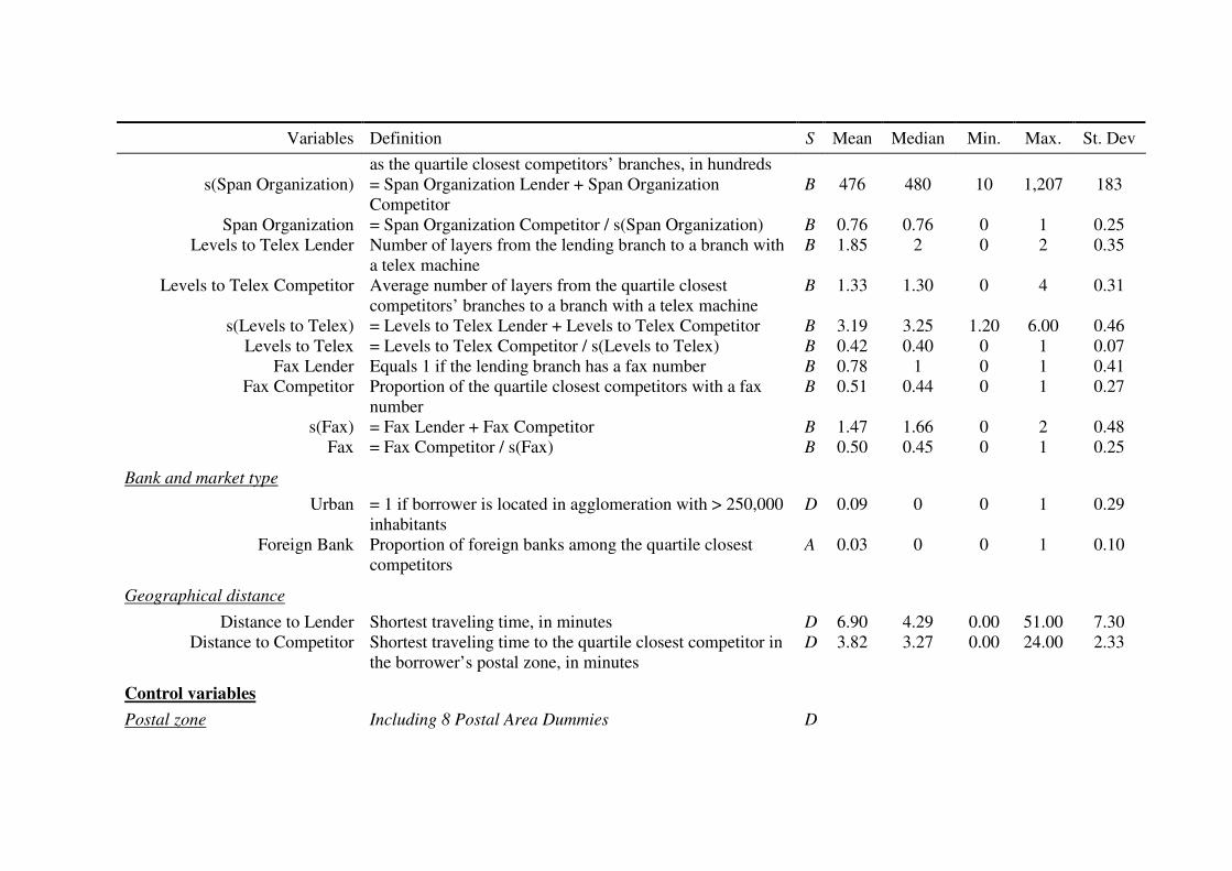
Variables Definition S Mean Median Min. Max. St. Dev

as the quartile closest competitors’ branches, in hundreds s(Span Organization) = Span Organization Lender + Span Organization

Competitor B 476 480 10 1,207 183

Span Organization = Span Organization Competitor / s(Span Organization) B 0.76 0.76 0 1 0.25 Levels to Telex Lender Number of layers from the lending branch to a branch with

a telex machine B 1.85 2 0 2 0.35

Levels to Telex Competitor Average number of layers from the quartile closest competitors’ branches to a branch with a telex machine

B 1.33 1.30 0 4 0.31

s(Levels to Telex) = Levels to Telex Lender + Levels to Telex Competitor B 3.19 3.25 1.20 6.00 0.46 Levels to Telex = Levels to Telex Competitor / s(Levels to Telex) B 0.42 0.40 0 1 0.07

Fax Lender Equals 1 if the lending branch has a fax number B 0.78 1 0 1 0.41 Fax Competitor Proportion of the quartile closest competitors with a fax

number B 0.51 0.44 0 1 0.27

s(Fax) = Fax Lender + Fax Competitor B 1.47 1.66 0 2 0.48 Fax = Fax Competitor / s(Fax) B 0.50 0.45 0 1 0.25

Bank and market type

Urban = 1 if borrower is located in agglomeration with > 250,000 inhabitants

D 0.09 0 0 1 0.29

Foreign Bank Proportion of foreign banks among the quartile closest competitors

A 0.03 0 0 1 0.10

Geographical distance

Distance to Lender Shortest traveling time, in minutes D 6.90 4.29 0.00 51.00 7.30 Distance to Competitor Shortest traveling time to the quartile closest competitor in

the borrower’s postal zone, in minutes D 3.82 3.27 0.00 24.00 2.33

Control variables

Postal zone Including 8 Postal Area Dummies D

Variables Definition S Mean Median Min. Max. St. Dev

Herfindahl-Hirschman Index Summed squares of bank market shares by number of branches in borrower’s postal zone

B 0.17 0.15 0.05 1 0.11

Number of Firms Number of registered firms in the borrower’s postal zone, in thousands

F 0.74 0.45 0.00 6.10 0.89

Relationship characteristics

Main bank = 1 if bank considers itself as main bank,a in percent D 58.82 100 0 100 49.22

Duration of Relationship Length of relationship with current lender, in years D 7.93 7.47 0.00 26.39 5.44

Contract characteristics Including 4 Loan Revisability Dummies D

Collateral = 1 if loan is secured via collateral, in percent D 26.40 0 0 100 44.08 Repayment Duration of Loan Repayment duration of loan, in years D 2.35 0.55 0.00 20.00 3.26

Loan purpose

Mortgage = 1 if loan is a business mortgage loan D n/ab Term = 1 if loan is a business term loan (investment credit) D n/ab

Securitizable term = 1 if loan is a securitizable business term loan (investment credit)

D n/ab

Bridge = 1 if loan is a bridge loan D n/ab Prepay taxes = 1 if loan is credit to prepay taxes D n/ab

Consumer credit = 1 if loan is a consumer credit loan (capturing installment loans)

D n/ab

Other = 1 if loan is given for another purpose or its purpose is not specified

D n/ab

Rollover = 1 if loan is given to prepay another loan, in percent D 10.20 0 0 100 30.27

Firm characteristics Including 49 Industry Dummies D

Small firm = 1 if < 10 employees and turnover < 250 mln. BEF,c in percent

D 15.99 0 0 100 36.64

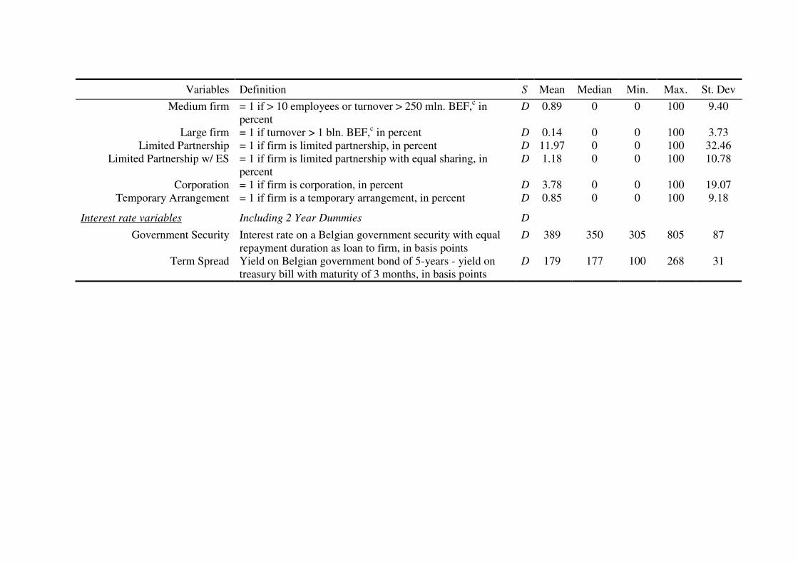
Variables Definition S Mean Median Min. Max. St. Dev

Medium firm = 1 if > 10 employees or turnover > 250 mln. BEF,c in percent

D 0.89 0 0 100 9.40

Large firm = 1 if turnover > 1 bln. BEF,c in percent D 0.14 0 0 100 3.73 Limited Partnership = 1 if firm is limited partnership, in percent D 11.97 0 0 100 32.46

Limited Partnership w/ ES = 1 if firm is limited partnership with equal sharing, in percent

D 1.18 0 0 100 10.78

Corporation = 1 if firm is corporation, in percent D 3.78 0 0 100 19.07 Temporary Arrangement = 1 if firm is a temporary arrangement, in percent D 0.85 0 0 100 9.18

Interest rate variables Including 2 Year Dummies D

Government Security Interest rate on a Belgian government security with equal repayment duration as loan to firm, in basis points

D 389 350 305 805 87

Term Spread Yield on Belgian government bond of 5-years - yield on treasury bill with maturity of 3 months, in basis points

D 179 177 100 268 31

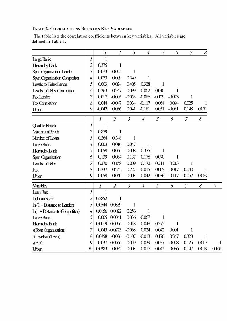
TABLE 2. CORRELATIONS BETWEEN KEY VARIABLES

The table lists the correlation coefficients between key variables. All variables are defined in Table 1.

1 2 3 4 5 6 7 8

Large Bank 1 1

Hierarchy Bank 2 0.375 1

Span Organization Lender 3 -0.073 -0.025 1

Span Organization Competitor 4 0.073 0.009 0.249 1

Levels to Telex Lender 5 0.003 0.024 0.405 0.328 1

Levels to Telex Competitor 6 0.263 0.347 -0.099 0.062 -0.010 1

Fax Lender 7 0.017 -0.005 -0.053 -0.086 -0.129 -0.073 1

Fax Competitor 8 0.044 -0.047 0.034 -0.117 0.064 0.094 0.025 1

Urban 9 -0.042 0.036 0.041 -0.181 0.051 -0.031 0.148 0.071

1 2 3 4 5 6 7 8

Quartile Reach 1 1

Maximum Reach 2 0.879 1

Number of Loans 3 0.264 0.348 1

Large Bank 4 -0.003 -0.016 -0.047 1

Hierarchy Bank 5 -0.059 -0.066 -0.008 0.375 1

Span Organization 6 0.139 0.084 0.137 0.178 0.070 1

Levels to Telex 7 0.270 0.158 0.209 0.172 0.211 0.213 1

Fax 8 -0.237 -0.242 -0.227 0.015 -0.005 -0.017 -0.040 1

Urban 9 0.059 0.040 -0.008 -0.042 0.036 -0.117 -0.057 -0.089

Variables 1 2 3 4 5 6 7 8 9

Loan Rate 1 1

ln(Loan Size) 2 -0.5852 1

ln (1 + Distance to Lender) 3 -0.0544 0.0859 1

ln(1 + Distance to Competitor) 4 0.0156 0.0022 0.256 1

Large Bank 5 0.005 0.0041 0.036 -0.067 1

Hierarchy Bank 6 -0.0019 0.0026 -0.018 -0.048 0.375 1

s(Span Organization) 7 0.045 -0.0273 -0.068 0.024 0.042 0.001 1

s(Levels to Telex) 8 0.0358 -0.026 -0.107 -0.013 0.176 0.247 0.328 1

s(Fax) 9 0.037 -0.0266 0.059 -0.039 0.037 -0.028 -0.125 -0.067 1

Urban 10 -0.0283 0.032 -0.008 0.017 -0.042 0.036 -0.147 0.019 0.162

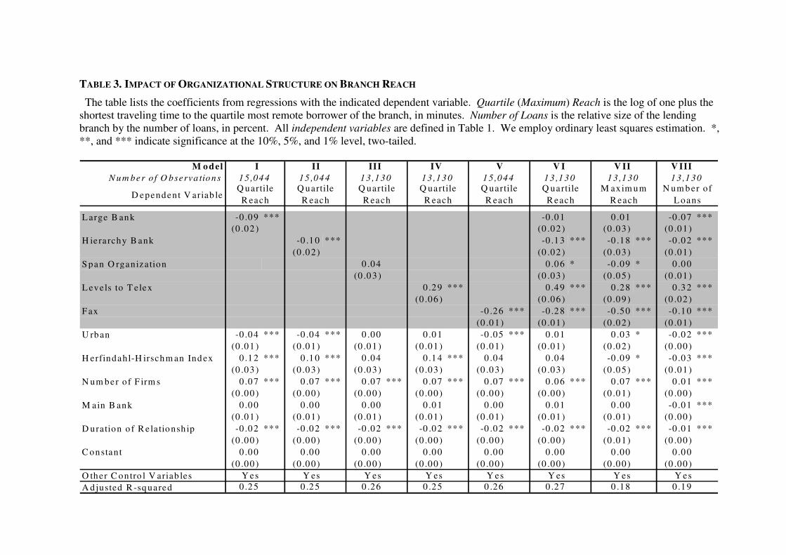
TABLE 3. IMPACT OF ORGANIZATIONAL STRUCTURE ON BRANCH REACH

The table lists the coefficients from regressions with the indicated dependent variable. Quartile (Maximum) Reach is the log of one plus the shortest traveling time to the quartile most remote borrower of the branch, in minutes. Number of Loans is the relative size of the lending branch by the number of loans, in percent. All independent variables are defined in Table 1. We employ ordinary least squares estimation. *, **, and *** indicate significance at the 10%, 5%, and 1% level, two-tailed.

M o del I II III IV V V I V II V III

N u m ber o f O bserva tio ns

D ependent V ariab le

L arge B ank -0 .0 9 *** -0 .0 1 0 .01 -0 .0 7 ***

(0 .02 ) (0 .02 ) (0 .0 3) (0 .01 )

H ierarchy B ank -0 .1 0 *** -0 .1 3 *** -0 .18 *** -0 .0 2 ***

(0 .0 2) (0 .02 ) (0 .0 3) (0 .01 )

S pan O rganization 0 .04 0 .0 6 * -0 .09 * 0 .0 0

(0 .0 3 ) (0 .03 ) (0 .0 5) (0 .01 )

L evels to T elex 0 .2 9 *** 0 .4 9 *** 0 .28 *** 0 .3 2 ***

(0 .06 ) (0 .06 ) (0 .0 9) (0 .02 )

F ax -0 .26 *** -0 .2 8 *** -0 .50 *** -0 .1 0 ***

(0 .0 1) (0 .01 ) (0 .0 2) (0 .01 )

U rb an -0 .0 4 *** -0 .0 4 *** 0 .00 0 .0 1 -0 .05 *** 0 .0 1 0 .03 * -0 .0 2 ***

(0 .01 ) (0 .0 1) (0 .0 1 ) (0 .01 ) (0 .0 1) (0 .01 ) (0 .0 2) (0 .00 )

H erfindahl-H irschm an Ind ex 0 .1 2 *** 0 .1 0 *** 0 .04 0 .1 4 *** 0 .04 0 .0 4 -0 .09 * -0 .0 3 ***

(0 .03 ) (0 .0 3) (0 .0 3 ) (0 .03 ) (0 .0 3) (0 .03 ) (0 .0 5) (0 .01 )

N um ber o f F irm s 0 .0 7 *** 0 .0 7 *** 0 .07 *** 0 .0 7 *** 0 .07 *** 0 .0 6 *** 0 .07 *** 0 .0 1 ***

(0 .00 ) (0 .0 0) (0 .0 0 ) (0 .00 ) (0 .0 0) (0 .00 ) (0 .0 1) (0 .00 )

M ain B ank 0 .0 0 0 .0 0 0 .00 0 .0 1 0 .00 0 .0 1 0 .00 -0 .0 1 ***

(0 .01 ) (0 .0 1) (0 .0 1 ) (0 .01 ) (0 .0 1) (0 .01 ) (0 .0 1) (0 .00 )

D uration o f R ela tio nsh ip -0 .0 2 *** -0 .0 2 *** -0 .02 *** -0 .0 2 *** -0 .02 *** -0 .0 2 *** -0 .02 *** -0 .0 1 ***

(0 .00 ) (0 .0 0) (0 .0 0 ) (0 .00 ) (0 .0 0) (0 .00 ) (0 .0 1) (0 .00 )

C onstant 0 .0 0 0 .0 0 0 .00 0 .0 0 0 .00 0 .0 0 0 .00 0 .0 0

(0 .00 ) (0 .0 0) (0 .0 0 ) (0 .00 ) (0 .0 0) (0 .00 ) (0 .0 0) (0 .00 )

O ther C ontro l V ariab les Y es Y es Y es Y es Y es Y es Y es Y es

A djusted R -sq uared 0 .2 5 0 .2 5 0 .26 0 .2 5 0 .26 0 .2 7 0 .18 0 .1 9

Q uartile

R each

M axim um

R each

Q uartile

R each

1 3 ,1 3015 ,04 4 1 3 ,1 30 13 ,13 01 5 ,04 4

Q uartile

R each

Q uartile

R each

Q uartile

R each

Q uartile

R each

1 3 ,1 301 5 ,0 44 1 3 ,1 3 0

N um b er o f

L oans

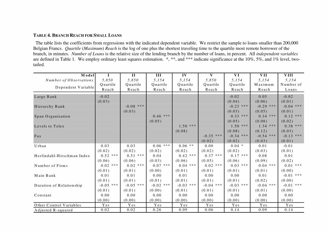
TABLE 4. BRANCH REACH FOR SMALL LOANS

The table lists the coefficients from regressions with the indicated dependent variable. We restrict the sample to loans smaller than 200,000 Belgian Francs. Quartile (Maximum) Reach is the log of one plus the shortest traveling time to the quartile most remote borrower of the branch, in minutes. Number of Loans is the relative size of the lending branch by the number of loans, in percent. All independent variables are defined in Table 1. We employ ordinary least squares estimation. *, **, and *** indicate significance at the 10%, 5%, and 1% level, two-tailed.

M o d el I II III IV V V I V II V III

N u m b er o f O b serva tio n s

D ep end ent V ariab le

L arge B ank -0 .0 2 -0 .0 2 0 .0 5 -0 .0 2

(0 .0 3 ) (0 .0 4 ) (0 .0 6 ) (0 .0 1 )

H ierarchy B ank -0 .0 8 *** -0 .2 3 *** -0 .2 9 *** -0 .0 4 ***

(0 .0 3 ) (0 .0 3 ) (0 .0 5 ) (0 .0 1 )

S p an O rgan iza tio n 0 .4 6 *** 0 .3 3 *** 0 .3 4 *** 0 .1 2 ***

(0 .0 5 ) (0 .0 5 ) (0 .0 8 ) (0 .0 2 )

L evels to T e lex 1 .5 0 *** 1 .5 0 *** 1 .3 4 *** 0 .3 8 ***

(0 .0 8 ) (0 .0 8 ) (0 .1 2 ) (0 .0 3 )

F ax -0 .3 5 *** -0 .3 4 *** -0 .5 4 *** -0 .1 3 ***

(0 .0 2 ) (0 .0 2 ) (0 .0 3 ) (0 .0 1 )

U rb an 0 .0 3 0 .0 3 0 .0 6 *** 0 .0 6 ** 0 .0 0 0 .0 4 * 0 .0 1 -0 .0 1

(0 .0 2 ) (0 .0 2 ) (0 .0 2 ) (0 .0 2 ) (0 .0 2 ) (0 .0 2 ) (0 .0 3 ) (0 .0 1 )

H erfind ah l-H irschm an Ind ex 0 .5 2 *** 0 .5 1 *** 0 .0 4 0 .4 2 *** 0 .3 7 *** 0 .1 7 *** 0 .0 8 0 .0 1

(0 .0 6 ) (0 .0 6 ) (0 .0 3 ) (0 .0 6 ) (0 .0 5 ) (0 .0 6 ) (0 .0 9 ) (0 .0 2 )

N um b er o f F irm s 0 .0 2 *** 0 .0 2 *** 0 .0 7 *** 0 .0 4 *** 0 .0 2 *** 0 .0 3 *** 0 .0 4 *** 0 .0 1 ***

(0 .0 1 ) (0 .0 1 ) (0 .0 0 ) (0 .0 1 ) (0 .0 1 ) (0 .0 1 ) (0 .0 1 ) (0 .0 0 )

M ain B ank 0 .0 1 0 .0 1 0 .0 0 0 .0 1 0 .0 0 0 .0 0 0 .0 1 -0 .0 1 ***

(0 .0 1 ) (0 .0 1 ) (0 .0 1 ) (0 .0 1 ) (0 .0 1 ) (0 .0 1 ) (0 .0 2 ) (0 .0 0 )

D ura tio n o f R ela tio nsh ip -0 .0 5 *** -0 .0 5 *** -0 .0 2 *** -0 .0 3 *** -0 .0 4 *** -0 .0 3 *** -0 .0 4 *** -0 .0 1 ***

(0 .0 1 ) (0 .0 1 ) (0 .0 0 ) (0 .0 1 ) (0 .0 1 ) (0 .0 1 ) (0 .0 1 ) (0 .0 0 )

C o nstan t 0 .0 0 0 .0 0 0 .0 0 0 .0 0 0 .0 0 0 .0 0 0 .0 0 0 .0 0

(0 .0 0 ) (0 .0 0 ) (0 .0 0 ) (0 .0 0 ) (0 .0 0 ) (0 .0 0 ) (0 .0 0 ) (0 .0 0 )

O ther C o ntro l V ariab les Y es Y es Y es Y es Y es Y es Y es Y es

A d justed R -sq uared 0 .0 2 0 .0 2 0 .2 6 0 .0 9 0 .0 6 0 .1 4 0 .0 9 0 .1 4

Q uartile

R each

Q uartile

R each

5 ,1 5 45 ,8 5 0 5 ,1 5 4

N um b er o f

L o ans

Q uartile

R each

M axim um

R each

Q uartile

R each

5 ,1 5 45 ,8 5 0 5 ,1 5 4 5 ,1 5 45 ,8 5 0

Q uartile

R each

Q uartile

R each

TABLE 5. INSTRUMENTAL VARIABLE ESTIMATION: ORGANIZATIONAL STRUCTURE AND BRANCH REACH

The table lists the coefficients from regressions with the indicated dependent variable. We instrument all independent variables indicated in italics with (1) a dummy that equals one if the postal zone is in and around Brussels, and for each postal zone (2) the average firm size in terms of total assets, (3) the average firm employment in terms of number of employees, (4) the average firm leverage, (5) the industry concentration index, and (6) a bank multi-market contact index. Quartile (Maximum) Reach is the log of one plus the shortest traveling time to the quartile most remote borrower of the branch, in minutes. Number of Loans is the relative size of the lending branch by the number of loans, in percent. All independent variables are defined in Table 1. We employ instrumental variable estimation. *, **, and *** indicate significance at the 10%, 5%, and 1% level, two-tailed.

M odel I II III IV V VI VII VIII

Number of Observations

Dependent Variable

Large Bank -0.06 *** -0.03 -0.02 -0.07 ***

(0.02) (0.02) (0.03) (0.01)

Hierarchy Bank -0.12 *** -0.25 *** -0.32 *** -0.02 ***

(0.02) (0.02) (0.03) (0.01)

Span Organization 0.50 *** 0.37 *** 0.35 *** 0.13 ***

(0.03) (0.03) (0.05) (0.01)

Levels to Telex 1.48 *** 1.50 *** 1.30 *** 0.36 ***

(0.05) (0.05) (0.07) (0.02)

Fax -0.36 *** -0.35 *** -0.55 *** -0.13 ***

(0.01) (0.01) (0.02) (0.00)

Urban 0.03 ** 0.04 *** 0.07 *** 0.07 *** 0.01 0.06 *** 0.03 -0.01 ***

(0.01) (0.01) (0.01) (0.01) (0.01) (0.01) (0.02) (0.00)

Herfindahl-Hirschman Index 0.51 *** 0.50 *** 0.04 0.38 *** 0.37 *** 0.15 *** 0.02 -0.01

(0.03) (0.03) (0.03) (0.03) (0.03) (0.03) (0.05) (0.01)

Number of Firms 0.03 *** 0.03 *** 0.07 *** 0.04 *** 0.03 *** 0.04 *** 0.04 *** 0.01 ***

(0.00) (0.00) (0.00) (0.00) (0.00) (0.00) (0.01) (0.00)

Main Bank -0.01 * -0.01 * 0.00 0.01 -0.02 *** 0.00 -0.01 -0.02 ***

(0.01) (0.01) (0.01) (0.01) (0.01) (0.01) (0.01) (0.00)

Duration of Relationship -0.04 *** -0.04 *** -0.02 *** -0.03 *** -0.04 *** -0.02 *** -0.03 *** -0.01 ***

(0.00) (0.00) (0.00) (0.01) (0.00) (0.00) (0.01) (0.00)

Constant 0.00 0.00 0.00 0.00 0.00 0.00 0.00 0.00

(0.00) (0.00) (0.00) (0.00) (0.00) (0.00) (0.00) (0.00)

Other Control Variables Yes Yes Yes Yes Yes Yes Yes Yes

Adjusted R-squared 0.03 0.04 0.26 0.10 0.07 0.16 0.10 0.13

F-Tests Instruments 446.03 *** 104.25 *** 104.84 *** 90.28 *** 83.94 ***

Quartile

Reach

Maximum

Reach

Quartile

Reach

13,11915,028 13,119 13,11915,028

Quartile

Reach

Quartile

Reach

Quartile

Reach

Quartile

Reach

13,11915,028 13,119

Number of

Loans

TABLE 6. BANKS’ ORGANIZATIONAL STRUCTURE AND THE SEVERITY OF SPATIAL PRICING

The table lists the coefficients from regressions with the Loan Rate until the next revision, in basis points, and 1,000 times the log of Loan

Size, in Belgian Francs, as the dependent variables. Distance to Lender is the shortest traveling time to the lender, in minutes. Distance to

Competitor is the shortest traveling time to the closest quartile competitor, in minutes. All other independent variables are defined in Table 1. We restrict the sample to loans smaller than 200,000 Belgian Francs (LS < 0.2) in Model VIII, and remove Brussels postal zones in Model IX (Outside Bxl). We employ ordinary least squares estimation. *, **, and *** indicate significance at the 10%, 5%, and 1% level, two-tailed.

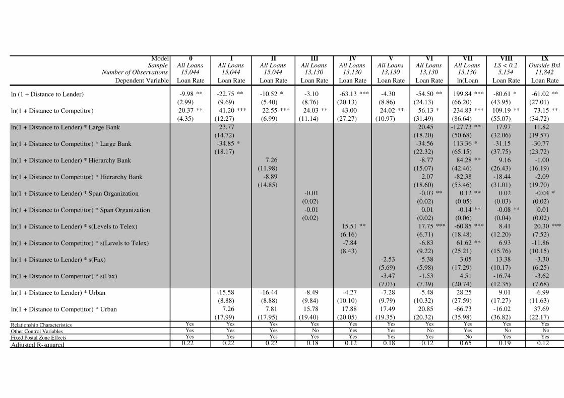
ModelSample

Number of Observations

Dependent Variable

ln (1 + Distance to Lender) -9.98 ** -22.75 ** -10.52 * -3.10 -63.13 *** -4.30 -54.50 ** 199.84 *** -80.61 * -61.02 **

(2.99) (9.69) (5.40) (8.76) (20.13) (8.86) (24.13) (66.20) (43.95) (27.01)

ln(1 + Distance to Competitor) 20.37 ** 41.20 *** 22.55 *** 24.03 ** 43.00 24.02 ** 56.13 * -234.83 *** 109.19 ** 73.15 **

(4.35) (12.27) (6.99) (11.14) (27.27) (10.97) (31.49) (86.64) (55.07) (34.72)

ln(1 + Distance to Lender) * Large Bank 23.77 20.45 -127.73 ** 17.97 11.82

(14.72) (18.20) (50.68) (32.06) (19.57)

ln(1 + Distance to Competitor) * Large Bank -34.85 * -34.56 113.36 * -31.15 -30.77

(18.17) (22.32) (65.15) (37.75) (23.72)

ln(1 + Distance to Lender) * Hierarchy Bank 7.26 -8.77 84.28 ** 9.16 -1.00

(11.98) (15.07) (42.46) (26.43) (16.19)

ln(1 + Distance to Competitor) * Hierarchy Bank -8.89 2.07 -82.38 -18.44 -2.09

(14.85) (18.60) (53.46) (31.01) (19.70)

ln(1 + Distance to Lender) * Span Organization -0.01 -0.03 ** 0.12 ** 0.02 -0.04 *

(0.02) (0.02) (0.05) (0.03) (0.02)

ln(1 + Distance to Competitor) * Span Organization -0.01 0.01 -0.14 ** -0.08 ** 0.01

(0.02) (0.02) (0.06) (0.04) (0.02)

ln(1 + Distance to Lender) * s(Levels to Telex) 15.51 ** 17.75 *** -60.85 *** 8.41 20.30 ***

(6.16) (6.71) (18.48) (12.20) (7.52)

ln(1 + Distance to Competitor) * s(Levels to Telex) -7.84 -6.83 61.62 ** 6.93 -11.86

(8.43) (9.22) (25.21) (15.76) (10.15)

ln(1 + Distance to Lender) * s(Fax) -2.53 -5.38 3.05 13.38 -3.30

(5.69) (5.98) (17.29) (10.17) (6.25)

ln(1 + Distance to Competitor) * s(Fax) -3.47 -1.53 4.51 -16.74 -3.62

(7.03) (7.39) (20.74) (12.35) (7.68)

ln(1 + Distance to Lender) * Urban -15.58 -16.44 -8.49 -4.27 -7.28 -5.48 28.25 9.01 -6.99

(8.88) (8.88) (9.84) (10.10) (9.79) (10.32) (27.59) (17.27) (11.63)

ln(1 + Distance to Competitor) * Urban 7.26 7.81 15.78 17.88 17.49 20.85 -66.73 -16.02 37.69

(17.99) (17.95) (19.40) (20.05) (19.35) (20.32) (35.98) (36.82) (22.17)Relationship Characteristics Yes Yes Yes Yes Yes Yes Yes Yes Yes Yes

Other Control Variables Yes Yes Yes No Yes Yes No Yes No No

Fixed Postal Zone Effects Yes Yes Yes Yes Yes Yes Yes No Yes Yes

Adjusted R-squared 0.22 0.22 0.22 0.18 0.12 0.18 0.12 0.65 0.19 0.12

0All Loans

15,044

Loan Rate

11,842

Loan Rate

IXOutside Bxl

5,154

Loan Rate

VIIILS < 0.2

I IVIII

ln(Loan

VII

13,130All LoansAll Loans All LoansAll Loans

Loan Rate

13,130

Loan Rate Loan Rate Loan RateLoan RateLoan Rate

15,044 13,130 13,130 13,13015,044

VIII VAll Loans All Loans All Loans

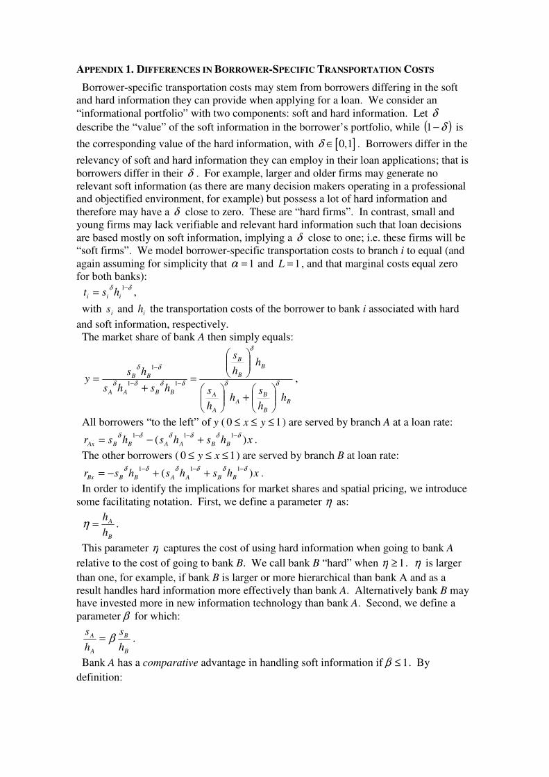
APPENDIX 1. DIFFERENCES IN BORROWER-SPECIFIC TRANSPORTATION COSTS

Borrower-specific transportation costs may stem from borrowers differing in the soft and hard information they can provide when applying for a loan. We consider an “informational portfolio” with two components: soft and hard information. Let δ

describe the “value” of the soft information in the borrower’s portfolio, while ( )δ−1 is

the corresponding value of the hard information, with [ ]0,1δ ∈ . Borrowers differ in the

relevancy of soft and hard information they can employ in their loan applications; that is borrowers differ in their δ . For example, larger and older firms may generate no relevant soft information (as there are many decision makers operating in a professional and objectified environment, for example) but possess a lot of hard information and therefore may have a δ close to zero. These are “hard firms”. In contrast, small and young firms may lack verifiable and relevant hard information such that loan decisions are based mostly on soft information, implying a δ close to one; i.e. these firms will be “soft firms”. We model borrower-specific transportation costs to branch i to equal (and again assuming for simplicity that 1=α and 1=L , and that marginal costs equal zero for both banks):

δδ −=

1

iii hst ,

with is and ih the transportation costs of the borrower to bank i associated with hard

and soft information, respectively. The market share of bank A then simply equals:

B

B

BA

A

A

B

B

B

BBAA

BB

hh

sh

h

s

hh

s

hshs

hsy

δδ

δ

δδδδ

δδ

+

=+

=−−

−

11

1

,

All borrowers “to the left” of y ( 10 ≤≤≤ yx ) are served by branch A at a loan rate:

xhshshsr BBAABBAx )(111 δδδδδδ −−−

+−= .

The other borrowers ( 10 ≤≤≤ xy ) are served by branch B at loan rate:

xhshshsr BBAABBBx )(111 δδδδδδ −−−

++−= .

In order to identify the implications for market shares and spatial pricing, we introduce some facilitating notation. First, we define a parameter η as:

B

A

h

h=η .

This parameter η captures the cost of using hard information when going to bank A

relative to the cost of going to bank B. We call bank B “hard” when 1≥η . η is larger

than one, for example, if bank B is larger or more hierarchical than bank A and as a result handles hard information more effectively than bank A. Alternatively bank B may have invested more in new information technology than bank A. Second, we define a parameter β for which:

B

B

A

A

h

s

h

sβ= .

Bank A has a comparative advantage in handling soft information if 1≤β . By

definition:

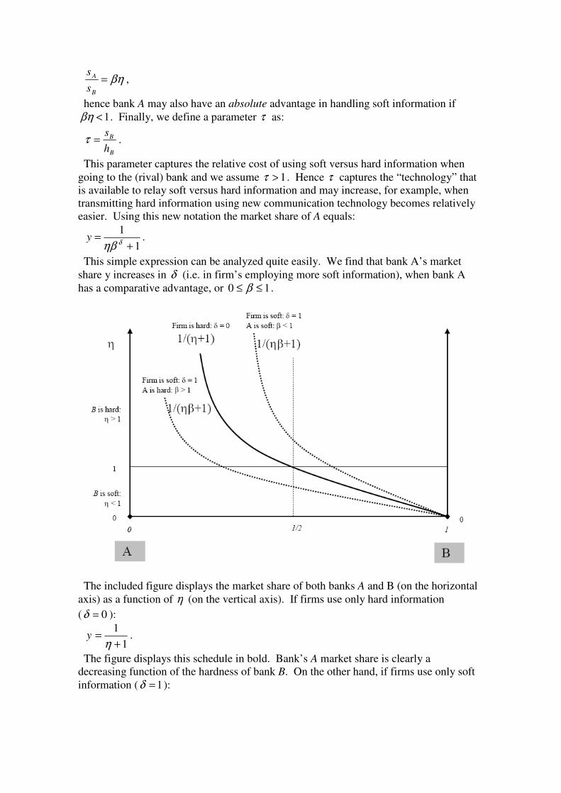
βη=B

A

s

s,

hence bank A may also have an absolute advantage in handling soft information if 1<βη . Finally, we define a parameter τ as:

B

B

h

s=τ .

This parameter captures the relative cost of using soft versus hard information when going to the (rival) bank and we assume 1>τ . Hence τ captures the “technology” that is available to relay soft versus hard information and may increase, for example, when transmitting hard information using new communication technology becomes relatively easier. Using this new notation the market share of A equals:

1

1

+=

δηβy .

This simple expression can be analyzed quite easily. We find that bank A’s market share y increases in δ (i.e. in firm’s employing more soft information), when bank A has a comparative advantage, or 10 ≤≤ β .

The included figure displays the market share of both banks A and B (on the horizontal

axis) as a function of η (on the vertical axis). If firms use only hard information

( 0=δ ):

1

1

+=

ηy .

The figure displays this schedule in bold. Bank’s A market share is clearly a decreasing function of the hardness of bank B. On the other hand, if firms use only soft information ( 1=δ ):

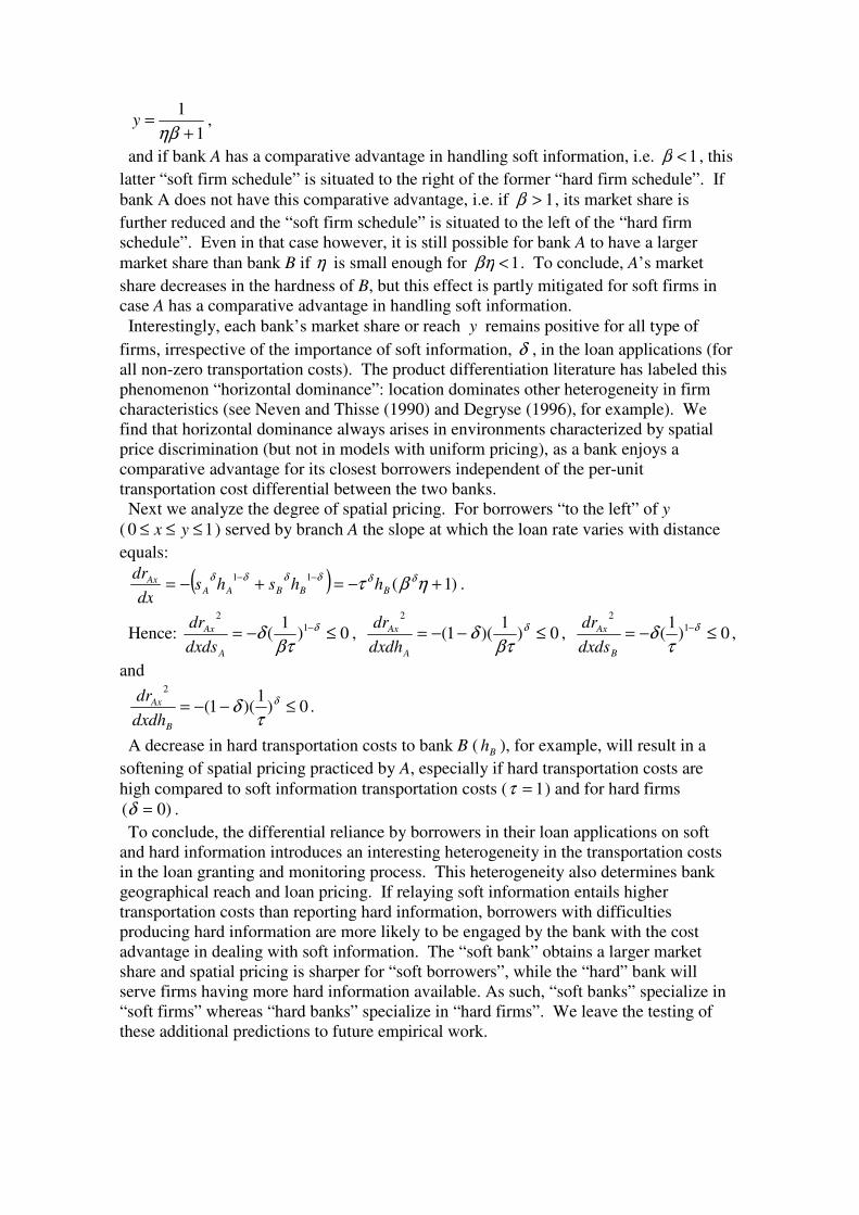
1

1

+=

ηβy ,

and if bank A has a comparative advantage in handling soft information, i.e. 1<β , this

latter “soft firm schedule” is situated to the right of the former “hard firm schedule”. If bank A does not have this comparative advantage, i.e. if 1>β , its market share is

further reduced and the “soft firm schedule” is situated to the left of the “hard firm schedule”. Even in that case however, it is still possible for bank A to have a larger market share than bank B if η is small enough for 1<βη . To conclude, A’s market

share decreases in the hardness of B, but this effect is partly mitigated for soft firms in case A has a comparative advantage in handling soft information. Interestingly, each bank’s market share or reach y remains positive for all type of

firms, irrespective of the importance of soft information, δ , in the loan applications (for all non-zero transportation costs). The product differentiation literature has labeled this phenomenon “horizontal dominance”: location dominates other heterogeneity in firm characteristics (see Neven and Thisse (1990) and Degryse (1996), for example). We find that horizontal dominance always arises in environments characterized by spatial price discrimination (but not in models with uniform pricing), as a bank enjoys a comparative advantage for its closest borrowers independent of the per-unit transportation cost differential between the two banks. Next we analyze the degree of spatial pricing. For borrowers “to the left” of y

( 10 ≤≤≤ yx ) served by branch A the slope at which the loan rate varies with distance

equals:

( ) )1(11

+−=+−=−−

ηβτ δδδδδδ

BBBAAAx hhshs

dx

dr.

Hence: 0)1

( 1

2

≤−= −δ

βτδ

A

Ax

dxds

dr, 0)

1)(1(

2

≤−−= δ

βτδ

A

Ax

dxdh

dr, 0)

1( 1

2

≤−= −δ

τδ

B

Ax

dxds

dr,

and

0)1

)(1(2

≤−−= δ

τδ

B

Ax

dxdh

dr.

A decrease in hard transportation costs to bank B ( Bh ), for example, will result in a

softening of spatial pricing practiced by A, especially if hard transportation costs are high compared to soft information transportation costs ( 1=τ ) and for hard firms

)0( =δ .

To conclude, the differential reliance by borrowers in their loan applications on soft and hard information introduces an interesting heterogeneity in the transportation costs in the loan granting and monitoring process. This heterogeneity also determines bank geographical reach and loan pricing. If relaying soft information entails higher transportation costs than reporting hard information, borrowers with difficulties producing hard information are more likely to be engaged by the bank with the cost advantage in dealing with soft information. The “soft bank” obtains a larger market share and spatial pricing is sharper for “soft borrowers”, while the “hard” bank will serve firms having more hard information available. As such, “soft banks” specialize in “soft firms” whereas “hard banks” specialize in “hard firms”. We leave the testing of these additional predictions to future empirical work.

APPENDIX 2. COEFFICIENTS OF CONTROL VARIABLES IN SELECTED SPECIFICATIONS

The table lists the coefficients from regressions with the indicated dependent variable. All variables are defined in Table 1. Light gray cells were already reported in the other tables. We employ ordinary least squares estimation. The number of observations equals 15,044. *, **, and *** indicate significance at the 10%, 5%, and 1% level, two-tailed.

M odel V I V II V III

N um ber o f O b serva tion s

D ep end ent V ariab le

L arge B ank -0 .0 1 0 .01 -0 .07 ***

H ierarchy B ank -0 .1 3 *** -0 .18 *** -0 .02 ***

S pan O rganiza tio n 0 .06 * -0 .09 * 0 .00

L evels to T elex 0 .49 *** 0 .28 *** 0 .32 ***

F ax -0 .2 8 *** -0 .50 *** -0 .10 ***

U rb an 0 .01 0 .03 * -0 .02 ***

H erfindahl-H irschm an Index 0 .04 -0 .09 * -0 .03 ***

N um b er o f F irm s 0 .06 *** 0 .07 *** 0 .01 ***

M ain B ank 0 .01 0 .00 -0 .01 ***

D ura tion o f R elatio nship -0 .0 2 *** -0 .02 *** -0 .01 ***

C olla teral 0 .06 *** 0 .07 *** -0 .04 ***

ln( 1 + R epaym ent D ura tio n o f Loan) 0 .03 0 .04 0 .00

M ortgage -0 .0 4 -0 .06 0 .05 ***

T erm -0 .0 5 * -0 .07 0 .09 ***

S ecuritizab le term -0 .0 8 * -0 .10 0 .05 ***

B rid ge -0 .0 7 0 .02 0 .03

P rep ay taxes -0 .4 4 -0 .49 0 .04

C onsum er c red it -0 .0 3 * -0 .04 ** 0 .02 ***

R ollo ver 0 .02 0 .05 ** 0 .00

T erm Spread -0 .0 3 ** -0 .05 ** -0 .01 **

C onstant 0 .00 0 .00 0 .00

8 P ostal A rea D um m ies Yes Yes Yes

4 L oan R evisab ility D um m ies Yes Yes Yes

4 9 Ind ustry D um m ies Yes Yes Yes

2 Y ear D um m ies Yes Yes Yes

A djusted R -sq uared 0 .27 0 .18 0 .19

N um ber o f

Lo ans

1 3 ,13 013 ,130

M axim um

R each

Q uartile

R each

13 ,1 30