NORTHWESTERN UNIVERSITY

The Impact of Information Sharing on Supply ChainPerformance

A DISSERTATION

SUBMITTED TO THE GRADUATE SCHOOLIN PARTIAL FULFILLMENT OF THE REQUIREMENTS

for the degreeDOCTOR OF PHILOSOPHY

Field of Industrial Engineering and Management Sciences

ByYao Zhao

EVANSTON, ILLINOISDecember 2002

c© Copyright by Yao Zhao 2008

All Rights Reserved

ii

ABSTRACT

The Impact of Information Sharing on Supply Chain

Performance

Yao Zhao

This thesis is motivated by the impact that information technology has had

on supply chain management. In particular, information technology has changed

the way companies interact with suppliers and customers. For example, in quick

response, suppliers receive Point-of-Sales (POS) data from retailers and use this

information to improve their forecast and better manage production and inventory

activities.

Our objective is to study the value of information sharing and how to effec-

tively utilize demand related information in supply chains. For this purpose, we

develop and analyze two models, the first one focuses on inventory cost reduction in

a two-stage supply chain where the manufacturer has a limited production capacity.

The second model characterizes the forecast accuracy improvement in a multi-stage

supply chain facing stationary and correlated demand.

The thesis starts by analyzing a periodic review, two-stage production-inventory

system with a single capacitated manufacturer and a single retailer facing stochas-

tic demand. The manufacturer receives demand information from the retailer even

during time periods in which the retailer does not place orders. Assuming a finite

time horizon, we characterize the optimal production-inventory policy for the man-

ufacturer, explore the policy structure, and study the optimal frequency and timing

in which information should be shared.

We then analyze a similar model in infinite time horizon. First, we provide a new

iii

and simple proof for the optimality of the cyclic order-up-to policy under average

cost criterion. Then, using Infinitesimal Perturbation Analysis (IPA) we quantify

the impact of information sharing, as well as the impact of the frequency and timing

of information sharing on the manufacturer’s performance.

In the last part of the thesis, we consider a distribution system with a single

manufacturer, a single distribution center and multiple non-identical retailers in

infinite time horizon. The retailers place orders periodically, the distribution center

transfers the aggregated orders from the retailers to the manufacturer. Assuming

stationary and correlated external demands, we quantify the impact of sharing the

order and demand information of individual retailers on the manufacturer’s forecast

accuracy.

iv

Acknowledgments

My first and foremost appreciation goes to my advisor, Professor David Simchi-

Levi, under whose guidance the thesis was written, for his superb mentorship and

continuous support throughout the course of this research. I am greatly inspired by

his work ethic and high standard. His passion for cutting-edge research combined

with profound intellectual integrity has always been a major source of support and

inspiration. While the friendship and the personal guidance that he offered me make

my long academia life very enjoyable, the industrial experiences that he guided me

through have deepened my thinking and enriched my academic life substantially. I

feel greatly privileged to be one of his students. Finally, David, I would like to thank

you for providing me the chance to visit MIT Operations Research Center (ORC).

I was so lucky to stay in two of the most exciting places of Industrial Engineering

and Operations Research. I will be benefiting from these experiences for the years

to come.

All of the faculty members in the Industrial Engineering and Management Sci-

ences Department earn my gratitude. In particular, I want to thank Professor Barry

Nelson for being a mentor over the past 4 years. He taught me stochastic processes

and simulation, provided hints for me for some of the proofs in Chapter 3, proof

v

read the entire thesis, and provided me ideas for future research. Barry is so knowl-

edgeable and willing to help at any time, it makes my feel so lucky to be a student

of IE/MS. I would also like to thank Professor Seyed Iravani, for providing the in-

sightful suggestions and making valuable comments on the dissertation. In addition,

Seyed has an open door and is always willing to share knowledge. I am very grate-

ful for the support and academic advice offered by our department chair, Professor

Ajit Tamhane. Ajit introduced me to the field of time series analysis, and provided

valuable comments on Chapter 4. Finally, I would like to thank Professor Yehuda

Bassok for his time and effort on my thesis. His support is greatly appreciated.

My thanks also go to the staff and the graduate students in IE/MS at North-

western University and Operations Research Center at MIT. In particular, I would

like to thank Xin Chen at ORC for helping me check my proofs, and my dear fellow

students Max Shen, Hui Liu, Mabel Chou, Julie Swann at IE/MS for the provoca-

tive research discussions. I would also like to thank the graduate students at both

IE/MS and ORC for their time and comments during my seminar talks.

Finally, my thanks go to my family: my wife, my parents and my boy, who is

now 6 months old. I am particularly indebted to my wife, I remember the days and

nights that we spent together in Chicago and Boston, .... Words are not enough to

express my appreciation for you, my dear. This thesis would not have been possible

without your love, understanding and support.

vi

Contents

Abstract iii

Acknowledgments v

1 Introduction 1

1.1 Background and motivation . . . . . . . . . . . . . . . . . . . . . . . 1

1.2 Objectives and contributions . . . . . . . . . . . . . . . . . . . . . . . 5

1.3 Literature review . . . . . . . . . . . . . . . . . . . . . . . . . . . . . 9

1.3.1 Batch ordering . . . . . . . . . . . . . . . . . . . . . . . . . . 10

1.3.2 Advance demand information strategies . . . . . . . . . . . . . 13

1.3.3 Correlated demand processes . . . . . . . . . . . . . . . . . . 14

1.3.4 Other sources . . . . . . . . . . . . . . . . . . . . . . . . . . . 16

1.3.5 Summary . . . . . . . . . . . . . . . . . . . . . . . . . . . . . 17

1.4 Structure of the thesis . . . . . . . . . . . . . . . . . . . . . . . . . . 18

2 A capacitated two-stage supply chain: finite time horizon 20

2.1 Models . . . . . . . . . . . . . . . . . . . . . . . . . . . . . . . . . . . 20

2.1.1 No information sharing . . . . . . . . . . . . . . . . . . . . . . 23

2.1.2 Information sharing with optimal policy . . . . . . . . . . . . 25

vii

2.1.3 The value of information sharing . . . . . . . . . . . . . . . . 30

2.1.4 Analysis of non-dimensional parameters . . . . . . . . . . . . . 33

2.1.5 Information sharing and the greedy policy . . . . . . . . . . . 34

2.2 Timing of information sharing . . . . . . . . . . . . . . . . . . . . . . 35

2.3 Computational results . . . . . . . . . . . . . . . . . . . . . . . . . . 39

2.3.1 The effect of information sharing on the optimal policy . . . . 41

2.3.2 The effect of capacity . . . . . . . . . . . . . . . . . . . . . . . 44

2.3.3 The effect of penalty cost . . . . . . . . . . . . . . . . . . . . 48

2.3.4 The effect of the number of information periods . . . . . . . . 49

2.3.5 Optimal timing for information sharing . . . . . . . . . . . . . 51

2.4 Conclusion . . . . . . . . . . . . . . . . . . . . . . . . . . . . . . . . . 57

3 A capacitated two-stage supply chain: infinite time horizon 59

3.1 The model . . . . . . . . . . . . . . . . . . . . . . . . . . . . . . . . . 60

3.2 Properties of cyclic order-up-to policy . . . . . . . . . . . . . . . . . . 64

3.3 A Markov decision process . . . . . . . . . . . . . . . . . . . . . . . . 72

3.3.1 Discounted cost criterion . . . . . . . . . . . . . . . . . . . . . 73

3.3.2 Average cost criterion . . . . . . . . . . . . . . . . . . . . . . 78

3.4 Computational results . . . . . . . . . . . . . . . . . . . . . . . . . . 79

3.4.1 Computational method . . . . . . . . . . . . . . . . . . . . . . 80

3.4.2 The effect of capacity . . . . . . . . . . . . . . . . . . . . . . . 81

3.4.3 The effect of frequency of information sharing . . . . . . . . . 83

3.4.4 Optimal timing for information sharing . . . . . . . . . . . . . 84

3.5 Conclusion . . . . . . . . . . . . . . . . . . . . . . . . . . . . . . . . . 86

viii

4 A multi-stage supply chain: forecast accuracy 88

4.1 The model . . . . . . . . . . . . . . . . . . . . . . . . . . . . . . . . . 90

4.2 Information sharing . . . . . . . . . . . . . . . . . . . . . . . . . . . . 94

4.3 No information sharing . . . . . . . . . . . . . . . . . . . . . . . . . . 95

4.4 Computational results . . . . . . . . . . . . . . . . . . . . . . . . . . 104

4.5 Discussion and conclusion . . . . . . . . . . . . . . . . . . . . . . . . 108

5 Proofs and technical details 111

5.1 Proof of Lemma 2.1 . . . . . . . . . . . . . . . . . . . . . . . . . . . . 111

5.2 Proof of Lemma 2.3 . . . . . . . . . . . . . . . . . . . . . . . . . . . . 112

5.3 Proofs of Chapter 3 . . . . . . . . . . . . . . . . . . . . . . . . . . . . 114

5.4 IPA in the case of information sharing . . . . . . . . . . . . . . . . . 122

5.5 IPA in the case of no information sharing . . . . . . . . . . . . . . . . 125

5.6 IPA and the timing of information sharing . . . . . . . . . . . . . . . 126

5.7 Proofs of Chapter 4 . . . . . . . . . . . . . . . . . . . . . . . . . . . . 127

References 130

ix

List of Tables

1 The impact of production capacity . . . . . . . . . . . . . . . . . . . 41

2 The impact of penalty cost . . . . . . . . . . . . . . . . . . . . . . . . 42

3 The impact of demand variability . . . . . . . . . . . . . . . . . . . . 43

4 Two ordering periods . . . . . . . . . . . . . . . . . . . . . . . . . . . 44

x

List of Figures

1 The impact of production capacity. . . . . . . . . . . . . . . . . . . . 45

2 The benefits of using information optimally. . . . . . . . . . . . . . . 46

3 Fill rates: the optimal policy vs. the greedy policy. . . . . . . . . . . 47

4 The impact of penalty cost . . . . . . . . . . . . . . . . . . . . . . . . 49

5 The impact of information sharing frequency. . . . . . . . . . . . . . . 50

6 The impact of the timing of information sharing. . . . . . . . . . . . . 51

7 Optimal timing for information sharing with different penalty cost. . 53

8 The impact of the timing of information sharing. . . . . . . . . . . . . 54

9 The impact of the timing of information sharing. . . . . . . . . . . . . 55

10 The impact of capacity and penalty cost on the optimal timing. . . . 56

11 The impact of the production capacity . . . . . . . . . . . . . . . . . 82

12 The impact of the frequency of information sharing . . . . . . . . . . 84

13 The impact of the timing of information sharing. . . . . . . . . . . . . 85

14 The impact of the transportation lead-time when |I | → ∞ . . . . . . 103

15 The impact of the number of retailers (K tends to infinity) . . . . . . 105

16 The impact of transportation lead-time (K tends to infinity) . . . . . 106

17 The averaged ratio of forecast errors . . . . . . . . . . . . . . . . . . 107

18 The 95% confidence interval of the ratio of forecast errors . . . . . . . 108

xi

Chapter 1

Introduction

1.1 Background and motivation

Information technology is an important enabler of efficient supply chain strategies.

Indeed, much of the current interest in supply chain management is motivated by the

possibilities introduced by the abundance of data and the savings inherent in sophis-

ticated analysis of these data. For example, information technology has changed the

way companies interact with suppliers and customers. Strategic partnering, which

relies heavily on information sharing, is becoming ubiquitous in many industries.

As observed by Stein and Sweat (1998), sharing demand related information

vertically among supply chain members has achieved huge impact in practice. Ac-

cording to Stein and Sweat, by ”exchanging information, such as Point of Sales

(POS), forecasting data, inventory level and sales trends, these companies are re-

ducing their cycle times, fulfilling orders more quickly, cutting out millions of dollars

in excess inventory, and improving customer service.”

To understand the impact of information sharing, consider traditional supply

chain strategies. Supply chains are highly complex systems with multiple production

1

2

and storage facilities. A typical supply chain consists of raw material suppliers,

assembly manufacturers, distributors and retailers. It is often managed in a decen-

tralized manner, i.e., each stage is managed based on information received from its

immediate suppliers and customers (decentralized information) and the objective of

the stage is to maximize profit with no, or very little regards, to its impact on other

stages in the supply chain (decentralized control). Thus, each stage makes locally

optimal decisions based on the orders placed by its customers, and the replenishment

lead time provided by its suppliers.

Such a decentralized information and control system faces significant challenges.

For example, ordering information flow may be distorted in the sense that the vari-

ation of orders tends to increase as one moves up the supply chain, a phenomenon

known as Bullwhip effect. The Bullwhip effect was first observed in practice by

companies such as Procter & Gamble and Hewlett-Packard, and later quantified by

Lee, Padmanabhan and Whang (1997a, b), and Chen, Drezner, Ryan and Simchi-

Levi (2000). Lee et al. identified the sources of Bullwhip effect to be: promotional

activities, inflated orders, order batching and price variation. Chen et al. (2000)

show that traditional forecasting methods such as moving average and exponential

smoothing also contribute to the increase in variability, that is, they also play an

important role in the bullwhip effect. They also show that transferring demand in-

formation across supply chain partners can significantly reduce the Bullwhip Effect

but it will never eliminate it.

The impact of the Bullwhip effect can be very significant. Indeed, the increase

in order variability implies that the firm needs to increase safety stock levels, or

otherwise service levels decrease. In addition, it is difficult to manage resources,

3

e.g., labor, equipment and transportation, effectively. More importantly, companies

are slow to respond to market changes because of the distortion in market signals.

The question, of course, is how to match demand and supply with minimal

inventory? In particular, the challenge is to do that in supply chains with long

production and transportation lead-times, and short product lifetime. To address

these challenges, a number of trends have emerged in supply chain strategies, all of

which take advantage of the abundance of information available in today’s supply

chains:

Quick Response: In this strategy, retailers share with the suppliers Point-Of-

Sales (POS), inventory levels and forecast data, as well as information on pro-

motional events. With the visibility of current demand and inventory levels,

suppliers can better forecast and schedule their production-inventory activi-

ties, and provide better service to their customers. Indeed, information sharing

can reduce the demand uncertainty to such an extent that suppliers can build

inventory well in advance of receiving a promotional order (Fahrenwaid, Wise

and Glynn, 2001). Of course, the ability of suppliers to prepare in advance

of an incoming order implies that they can reduce lead-times to the retailers.

This, together with an improved fill rate, allows retailers to reduce inventory

levels and the Bullwhip Effect, see Chen et al. (2000). For example, Milliken

and Company, a U.S. based textile and chemicals manufacturer, asked its retail

partners not only to provide the manufacturer, Milliken and Company, with

demand information, but also to provide the same information to its suppliers,

so that Milliken and Company can synchronize its production schedule with

its suppliers. This allowed Milliken and Company to reduce replenishment

4

lead-time to its retailers from 18 weeks to 3 weeks (Simchi-Levi, Kaminsky

and Simchi-Levi, 1999).

Collaborative Planning, Forecasting and Replenishment (CPFR): Many

companies not only share information with their supply chain partners, but

also jointly make decisions to improve supply chain performance. Specifically,

in CPFR, companies share information and also collaborate on forecasts, pro-

motional activities and production strategies. One of the most cited examples

is that of Wegmans grocery chain and Nabisco. The two companies use CPFR

on 22 items. Nabisco sales force developed a forecast for these items, which was

compared with Wegmans’ own forecasts. The pilot was successful: Nabisco

sales grew by 31%, while Wegmans sales increased by 16% with a surprising

18% decrease in inventory.

Henkel, the worldwide manufacturer of adhesives, consumer brand name prod-

ucts and industrial specialties, collaborates with its customer Eroski, Spain’s

largest food distribution group, by combining their complementary knowledge

of the market. In particular, Eroski brought to the partnership its understand-

ing of sales dynamics and promotions, while Henkel provided an expertise on

its products. Thus, Eroski focused more on the impact of promotion on sales,

while Henkel focused more on synchronizing demand planning with its produc-

tion planning. By integrating information of promotion, new product introduc-

tion and local activities into one forecast, these companies increased forecast

accuracy, improved customer service and reduced inventory level (Fahrenwaid,

Wise and Glynn, 2001).

5

Vendor Managed Inventory (VMI): A different type of collaboration between

retailers and suppliers based on information sharing is VMI. In this strategy,

the supplier determines not only her production schedule, but also the ship-

ments and inventory policies at retail facilities. Thus, VMI is a centralized

control strategy, in which the objective is to optimize decisions for the entire

supply chain. We refer readers to Simchi-Levi, Kaminsky and Simchi-Levi

(1999) for more details.

All these trends have one thing in common: they require retailers to transfer

demand information to their suppliers, and sometimes even to their suppliers’ sup-

pliers. However, sharing information also posses significant challenges. As reviewed

in Lee and Whang (1998), the challenges include: incentive issues, confidentiality

of the information shared, anti-trust regulations, reliability and cost of information

technology, the timeliness and accuracy of the shared information, and finally the

development of capabilities that allow companies to utilize the shared information

in an effective way.

In this thesis we focus on Quick Response. Our objective is to quantify the

benefits of information sharing and identify strategies that allow companies to utilize

information in an effective way. Evidently, an important related challenge, also

addressed in this thesis, is associated with the frequency and timing of information

sharing.

1.2 Objectives and contributions

The second and third chapters of this thesis are motivated by the Milliken and

Company example described earlier. As observed, Milliken and Company reduced

6

replenishment lead-time to the department stores from 18 weeks to 3 weeks by imple-

menting Quick Response. Although the underlying intuition is clear, i.e., demand

information can help suppliers better prepare for incoming orders, issues such as

when information sharing provides significant cost savings and how manufacturers

can use this information most effectively in a make-to stock production system, are

not well understood.

To address these issues, we considered a two-stage supply chain with a single

manufacturer having a finite production capacity and a single retailer facing inde-

pendent demand. The manufacturer produces to stock and the retailer manages her

inventory using an order-up-to inventory policy. Because many companies place or-

ders periodically while they can share information with their partners continuously,

we assume that the manufacturer can receive demand information from the retailer

even during time periods in which the retailer doesn’t place orders.

Specifically, we assume that the retailer has a fixed ordering interval. That

is, every T time periods, e.g., four weeks, the retailer places an order to raise his

inventory position to a certain level. The manufacturer receives demand information

from the retailer every τ units of time, τ ≤ T . For instance, the retailer places

an order every four weeks but provides demand information every week. This is

clearly the case in many retailer-manufacturer partnerships in which orders are

placed by the retailer at certain points in time but POS data is provided every day

or every week. In all these cases, POS data is provided to the manufacturer more

frequently than retailer orders. We refer to the time between successive orders as

the ordering period and the time between successive information sharing as the

information period. Of course, in most supply chains, information can be shared

7

almost continuously, e.g., every second, while decisions are made less frequently, e.g.,

every week. Thus, information periods really refers to the time interval between

successive use of the information provided.

Our objective is to characterize the benefit of information sharing for the man-

ufacturer, as well as to understand what can be done to make information sharing

most beneficial, e.g. how frequently should information be shared and when should

it be shared so that the manufacturer can realize the potential benefits.

For this purpose, we analyze the model in a finite time horizon and in an in-

finite time horizon setting. Throughout the thesis, we compare the following two

strategies. In the first strategy, referred to as no information sharing, the retailer

does not share information with the manufacturer except for orders. In the second

strategy, referred to as information sharing with optimal policy, the retailer

shares demand information with the manufacturer at the end of each information

period. We assume that the manufacturer knows the external demand distribution

for each information period, and uses an optimal strategy to schedule production

so as to minimize his own expected holding and shortage cost. For the finite horizon

model, we also considered a third strategy, referred to as information sharing

with greedy policy. In this strategy, the retailer shares demand information with

the manufacturer just as in the previous strategy, but instead of the optimal policy,

the manufacturer uses an heuristic that is easy to implement in practice, based on

demand and shortage in the previous information period, as well as his production

capacity.

This part of the thesis makes the following contributions:

8

• For the finite horizon case we characterize the structure of the optimal pro-

duction inventory policy.

• For the infinite horizon case we characterize the optimal production-inventory

policy under both discounted and average cost criteria. In particular, we

provide a new and simple proof for the optimality of the cyclic order-up-to

policy under average cost criterion.

• Using a computational study, we report on the impact of information sharing

on the manufacturer’s cost as a function of the production capacity and the

frequency and timing in which demand information is transferred from the

retailer to the manufacturer.

The fourth chapter of this thesis considers a simple distribution system with a

single manufacturer, a single cross-docking distribution center (DC) and multiple

retailers. In such a system, the retailers place orders to the DC, the DC aggregates

the orders from various retailers and transfers the orders to the manufacturer. This

chapter is motivated by our observation that many manufacturing companies gen-

erate forecast only based on the history of aggregated orders received from DCs.

That is, typically manufacturers do not utilize demand and order information of

individual retail stores when generating forecasts. This is the case either because

the information is not available to the manufacturer or because the benefits of these

information is not clear even if they are readily available.

For example, we are aware of a cosmetic manufacturing company that generates

forecast for its manufacturing facilities only based on the aggregated orders placed

by distribution centers, which in turn serve some 2000 retail stores. Interestingly

9

enough, in this case the demand and order information of individual retail stores is

available to the forecaster but, for some reason, the manufacturer chooses to ignore

the available information.

Assuming stationary and correlated external demands, we analyze the follow-

ing two cases: In the first case, which we refer to as no information sharing, the

manufacturer only receives the aggregated orders from the distribution center. In

the second case, which we refer to as information sharing, the manufacturer not

only receives the aggregated orders, but also the order and demand information of

individual retailers. Our objective is to quantify the impact of information sharing

on the manufacturer’s forecast accuracy.

This part of the thesis makes the following contributions:

• We analyze the impact of information sharing on the manufacturer’s forecast

accuracy, and compare it to the forecast accuracy without information sharing.

• Using a computational study, we report on the impact of information shar-

ing on the manufacturer’s forecast accuracy as a function of the number of

retailers, transportation lead-time and the number of historical data included

in determining the forecast.

1.3 Literature review

In this section we review the literature on models involving information sharing and

its impact on supply chain partners. We focus on

• Batch Ordering Models

• Advance Demand Information Strategies

10

• Correlated Demand Models

• Models that involve Promotional Activities

1.3.1 Batch ordering

Chen and Zheng (1997) compare the optimal installation stock and echelon stock

policies for a simple two-stage serial system with batch ordering. In an installation

stock policy, the inventory policy of each facility is determined so as to minimize the

expected supply chain cost, thus the supply chain is under centralized control. But

each stage is managed based on the corresponding policy using only local informa-

tion available to this stage (local information). In an echelon inventory policy, while

the objective remains the same, each stage is managed using information from all

of its downstream facilities (centralized information). Chen and Zheng observe that

the value of centralized stock information is insignificant for their test examples.

Similarly, Chen (1998) studies multi-stage serial production-inventory systems, and

compares the optimal echelon inventory policy (centralized information) with the

optimal installation inventory policy (local information). Assuming i.i.d. external

demand, Chen shows that the benefit of centralized information is 0-9% with a

average of 1.75%, and the benefit increases as lead-times and batch sizes increase.

Cachon and Fisher (2000) study the impact of centralized information on a peri-

odic review single supplier and multi-retailer system under centralized control. They

compared the following three strategies: first, no demand and inventory information

is shared between the retailers and the supplier, and the supplier uses first come

first serve (FCFS) principle to satisfy retailers’ orders. In the second strategy, each

time retailers place orders, they also transfer inventory information to the supplier

11

so that the supplier can choose an effective inventory allocation scheme. The third

strategy allows the retailers to transfer inventory information to the supplier each

time period, independent of whether an order is made. This information allows

the supplier to better manage its own inventory as well as more effectively allocate

inventory among the different retailers. Using a computational study, they report

that the gap between the first strategy and the third strategy is 2.2% on average,

and can be as high as 12%. Cachon and Fisher concludes that the benefits of infor-

mation sharing is small, while the benefits of automating transactions maybe much

larger since it helps reducing the lead-times and batch sizes.

Gallego, et al. (2001) consider a decentralized controlled system with one sup-

plier and one retailer. In a decentralized control system each party optimizes deci-

sions by looking at its own costs. The supplier, however, is charged with a penalty

costs proportional to its backlogged level. The supplier uses a base-stock policy

while the retailer uses a (Q, r) policy. All policies are continuously reviewed. With

continuous information sharing, the supplier knows exactly the retailer’s inventory

position at any time. She can reduce her cost by delaying her orders until the re-

tailer’s inventory position drop to a certain level. Thus, the supplier can obtain

substantial benefits from information sharing, while the retailer maybe slightly bet-

ter off, or even worse off due to the delayed supplier lead-time.

Another paper focusing on decentralized controlled distribution system is by

Aviv and Federgruen (1998). They analyze a single supplier multi-retailer system

where retailers face random demand and share inventories and sales data with the

supplier. Since it is quite difficult to find the optimal policy for the entire system,

these authors use heuristics. Specifically, they analyze the effectiveness of a VMI

12

program where sales and inventory data is used by the supplier to determine the

timing and the amount of shipments to the retailers. For this purpose, they compare

the performance of the VMI program with that of a traditional, decentralized system,

as well as a supply chain in which information is shared continuously, but decisions

are made individually, i.e., by the different parties. Their focus in the three systems

analyzed is on minimizing long-run average cost. Aviv and Federgruen report that

information sharing reduces system wide cost by 0% to 5% while VMI reduces cost,

relative to information sharing, by 0.4% to 9.5% and on average by 4.7%. They

also show that information sharing provides substantial benefits for the supplier,

but almost zero benefits for the retailers.

So far, all the papers either report limited benefits of information sharing for

the entire supply chain under centralized control, or substantial benefits but only

for the supplier under decentralized control. Cheung and Lee (2002) shows that

it is possible to design policies to take advantage of the shared information and

bring substantial benefits for both the supplier and the retailers in a decentralized

distribution system. Specifically, they show how information sharing can help the

supplier better coordinate shipments and rebalance the inventory level among a

number of retailers in a single supplier/multi-retailer system. They assume that

each partner uses continuous review (Q, r) policies, and the supplier and retailers

are located in a close proximity so that a single truck can serve all retailers in one trip.

By receiving demand and inventory information from the retailers, the supplier can

send out a shipment whenever the accumulative demand from all retailers reaches the

truck load. Their computational results show that utilizing the shared information

in this way can reduce both the retailers’ and the supplier’s inventory holding costs

13

without increasing transportation cost.

The papers described above consider the impact of information sharing on the

entire system. Gavirneni, Kapuscinski and Tayur (1999) focuses exclusively on the

party receiving the information. They analyze a simple two-stage supply chain with

a single capacitated supplier and a single retailer. In this periodic review model,

the retailer makes ordering decisions every period, using an (s, S) inventory policy,

and transfers demand information to the manufacturer every period, independent of

whether an order is made. Assuming the retailer can acquire from another supplier

any part of the order that manufacturer can not satisfy, they show that the benefit,

i.e., the supplier cost savings, due to information sharing, increases as production

capacity increases and it ranges from 1% to 35%.

1.3.2 Advance demand information strategies

Advance demand information strategies have been used in practice and analyzed in

academia for quite some time. Hariharan and Zipkin (1995) studied a single-stage

inventory system in which customers place orders well ahead of their due date.

Hariharan and Zipkin refer to the time between the placement of the order and the

due date as the customer lead-time. They show that the customer lead-time has the

exact opposite effect as that of replenishment lead-time. That is, the effect of longer

customer lead time is identical to the impact of shorter replenishment lead time.

Gallego and Ozer (2001) extend this idea to allow customers to place partial

orders ahead of the due date. The customers can modify but cannot cancel the

orders as the due date draw closer. The problem is then modeled as a Markov De-

cision Process (MDP) with state space of multiple dimensions. Assuming unlimited

14

production capacity, they find that a state dependent (s, S) or a base-stock policy

are optimal depending on whether the model incorporates setup cost. They quan-

tify the benefits of advance demand information through a numerical study and find

that system performance can be improved as customers place orders further into the

future. This is, of course, quite intuitive: since future demand is partially known,

demand uncertainty is significantly reduced.

Ozer and Wei (2001) extend the results above to include finite production ca-

pacity. They report that a state dependent modified base-stock policy is optimal

under discounted cost criterion if there is no setup cost. If the setup cost is non-zero,

a heuristic policy, first introduced by Gallego and Wolf (2000), is utilized: either

produce up-to full capacity or nothing. Using a computational study, Ozer and Wei

report the benefits of advance demand information and observe that the benefit

increases as capacity utilization increases.

Chen (2001) integrates advance demand information with price discounts by

assuming that customers are willing to accept longer delays if the supplier offers

price discounts in return. He discusses how such price discounts should be given,

how firms should make use of the advance demand information to manage inventory,

and what are the advantages and disadvantages of this strategy, both from revenue

and inventory cost points of views.

1.3.3 Correlated demand processes

All the models reviewed so far assume independent demand processes. A number of

recent papers quantify the benefits of information sharing when the external demand

is correlated in time.

15

Lee, So and Tang (2000) consider a two-stage supply chain with a single man-

ufacturer and a single retailer. In their model, external demand follows an AR(1)

process, and the supply chain members use periodic review base-stock policies. Ob-

serve, that since the demand process is not i.i.d., the retailer’s base-stock levels may

vary from period to period. They considered a traditional model without informa-

tion sharing as well as a model in which the retailer transfers demand, inventory

policy and forecast data to the manufacturer each time she (the retailer) places an

order. They make two important assumptions: (i) the retailer can return excessive

inventory to the manufacturer without charge if her inventory position is higher

than the target base-stock level, and (ii) the manufacturer is not able to utilize the

order history to calculate the actual demand. Under these assumptions, they report

that information sharing can help the manufacturer reduce inventory cost substan-

tially. The percentage cost saving increases as demand correlation or transportation

lead-time between the supplier and the retailer increases.

Raghunathan (2001) points out the weakness of the assumption that the supplier

is not able to utilize the order history to calculate actual demand. He argues that

information sharing has zero benefit if the supplier is intelligent enough so that it can

retrieve all the demand information from the order history given that it knows the

retailer’s inventory control policy. Thus, he concludes that only sharing information

of unexpected events, e.g. promotion, is beneficial.

Finally, Aviv (2002) explores the value of sharing market signals in a two-stage

distribution system, where a single supplier serves multiple retailers. Market signals

are defined to be the portion of demand uncertainty observable in advance, e.g.,

the impact of weather or promotion on demand. Furthermore, the demand process

16

can be characterized by a linear regressional form that depends on early market

signals. He discusses and compares the following three supply chain configurations:

In the first setting, the supplier and retailers coordinate their policy parameters in

order to minimize system-wide costs, but they do not share their observed market

signals. In the second setting, the supplier uses VMI without receiving the market

signals observed by the retailers. In the third setting, all demand related information

are shared between the supplier and the retailers in addition to the VMI strategy.

Assuming an AR(1) external demand process, Aviv demonstrates through numerical

examples that sharing market signals will likely be more beneficial for the entire

supply chain as demand correlation increases, and as companies are able to explain

larger portion of demand uncertainty.

1.3.4 Other sources

So far customer demand was modeled as exogenously determined stochastic process.

Iyer and Ye (2000) study the impact of sharing promotion related information, e.g.,

the timing of retail promotion, on a decentralized controlled supply chain with a

single retailer and a single manufacturer. In their model, the retailer can choose a

pricing scheme to maximize her expected profits and customer demand is assumed

to be sensitive to price. The manufacturer uses all information available to generate

an inventory policy that maximizes her expected profits subject to the service-level

requirement. Iyer and Ye observe that (1) if the retailer does not share promotion

related information with the manufacturer, the increased fluctuation in demand

will decrease the manufacturer’s profits; (2) if the retailer shares promotion related

information with the manufacturer, then both the retailer and the manufacturer can

17

benefit from promotions.

Finally, it is appropriate to observe that all the literature reviewed so far focuses

on information sharing from the downstream facilities to an upstream facility. Re-

cently, Yu and Chen (2001) study the impact of sharing supply related information,

e.g., production schedule, from an upstream to a downstream facility. The basic idea

is to use information as a tool to reduce supply uncertainty, and hence safety stock

at the downstream facility. Specifically, Yu and Chen study a single supplier and

single retailer system, in which the supplier makes her production schedule visible

to the retailer so that the retailer can better estimate the lead time for each order.

They compare this system with a traditional system without information sharing

and show that the retailer can achieve substantial cost savings from information

sharing.

1.3.5 Summary

To summarize, research on the benefits of information sharing and supply chain

collaboration is still in its early stage. Significant achievements have been made,

while many issues are still not well understood. For instance, what is the impact

of information sharing on a supplier with limited production capacity? How can

suppliers use the shared information most effectively in a quick response type of

partnership? In particular, how often should information be shared? If information

cannot be used continuously, when should it be shared? More importantly, how

can a capacitated supplier take advantage of the information shared even at times

when orders are not placed? And finally, how can suppliers improve their forecast

accuracy by using the demand and order information of individual retailers in a

18

multi-retailer distribution system? Some of these questions are answered in this

thesis.

1.4 Structure of the thesis

The thesis is organized as follows: In Chapter 2, we study a single product, periodic

review, two-stage production-inventory system with a single manufacturer and a

single retailer in a finite time horizon. The manufacturer has finite production ca-

pacity and the retailer faces independent demand. Assuming that the manufacturer

can receive demand information from the retailer even during time periods in which

the retailer does not place orders, we characterize the optimal production-inventory

policy for the manufacturer, and quantify the impact of information sharing on the

manufacturer’s cost and service level.

In Chapter 3, we analyze a similar model in an infinite time horizon. We provide

a new and simple proof for the optimality of the cyclic order-up-to policy under

average cost criterion. Using extensive computational analysis, we quantify the

impact of information sharing as well as the impact of the frequency and timing of

information sharing on the manufacturer’s performance.

Finally, in Chapter 4, we consider a single product distribution system with a

single manufacturer, a single distribution center and multiple retailers in infinite

time horizon. The retailers place orders periodically and use an order-up-to policy

to control their inventory. The distribution center serves as a cross docking point

and transfers the aggregated orders from the retailers to the manufacturer. Assum-

ing stationary and correlated external demands, we compare a supply chain with

information sharing to a supply chain without information sharing. When there is

19

no information sharing the manufacturer’s forecast is based on the historical data

of aggregated orders received from the DC. In a system with information sharing,

the manufacturer’s forecast is based on the historical data of external customer’s

demand as well as orders from each retailer. Using an analytic and a computational

study, we quantify the impact of information sharing on the manufacturer’s forecast

accuracy.

The results described in this thesis appear in Simchi-Levi and Zhao (2001a),

Simchi-Levi and Zhao (2001b), and Simchi-Levi and Zhao (2002).

Chapter 2

A capacitated two-stage supplychain: finite time horizon

In this chapter, we consider the simple two-stage supply chain in a finite time hori-

zon. Our objective is not only to characterize the benefit of information sharing, but

also to understand what can be done to make information sharing most beneficial,

e.g. how frequently should information be shared and when should it be shared so

that the manufacturer can realize the potential benefits.

This chapter is organized as follows: In Section 2.1, we set up the models for the

three strategies described in Chapter 1. In addition, we identify the policies used

by the manufacturer, discuss their properties and show the value of information

sharing. In Section 2.2, the optimal timing of information sharing is discussed. In

Section 2.3, we compare the performance of the three strategies using a numerical

study. Section 2.4 concludes the chapter.

2.1 Models

We consider a single product, periodical review, two-stage system with a single

retailer and a single manufacturer. External demand faced by the retailer every

20

21

information (ordering) period is an i.i.d. random variable. To simplify the analysis,

we assume that the retailer controls her inventory position (outstanding order plus

on-hand inventory minus backorder) by an order-up-to policy with constant order-

up-to level, i.e., in every ordering period, the retailer raises her inventory position

to a constant level. All unsatisfied demand at the retailer is backlogged, thus the

retailer transfers external demand of each ordering period to the manufacturer.

The manufacturer has a production capacity limit, i.e., a limit on the amount the

manufacturer can produce per unit of time. The manufacturer runs her production

line always at the full capacity limit. Our objective is to compare the performance

of the three strategies (see Chapter 1) in a finite time horizon.

The sequence of events in our model is as follows. At the beginning of an ordering

period the retailer reviews her inventory and places an order to raise the inventory

position to the target inventory level. The manufacturer receives the order from

the retailer, fills the order as much as she can from stock, then makes a production

decision. If the manufacturer cannot satisfy all of a retailer’s order from stock,

then the missing amount is backlogged. The backorder will not be delivered to the

retailer until the beginning of the next ordering period. Notice that changing the

manufacturer’s policy may affect the manufacturer’s service level, thus the retailer’s

performance. It will be interesting to study the impact of information sharing on the

entire system with both the manufacturer and the retailer. This problem may involve

incentive issues and coordination between the manufacturer and the retailer, which

we would like address in future studies. In this thesis, we choose to focus exclusively

on the manufacturer and assume that the retailer can adjust her order-up-to level

to meet her objectives. Finally, transportation lead-time between the manufacturer

22

and the retailer is assumed to be zero. Similarly, at the beginning of an information

period, the retailer transfers the POS data of the previous information period to the

manufacturer. Upon receiving this demand information, the manufacturer reduces

this demand from her inventory position although she still holds the stock, then

makes a production decision.

Throughout this chapter, we equally divide each ordering period into an integer

number of information periods unless otherwise mentioned. Thus, N = T/τ is an

integer and it represents the number of information periods in one ordering period.

We index information periods within one ordering period 1, 2, . . . , N where N is

the first information period in the ordering period and 1 is the last. Let C denote

the production capacity per information period, τ , while C denotes the production

capacity per ordering period, T . Hence, C = NC . Finally, c denotes the production

cost per item.

Since we calculate inventory holding cost for each information period, we let h be

the inventory holding cost per unit product per information period. Let 0 < β ≤ 1

be the time discount factor for one information period, evidently, one unit of product

kept in inventory for n information periods, n = N, N − 1, . . . , 1, will incur a total

inventory cost hn = h(1 + β + · · · + βn−1). To keep the consistency of notation, let

h0 = 0. It’s easy to see that the earlier the manufacturer makes a production run in

one ordering period, the longer she will carry the inventory, thus the more holding

cost she will have to pay. Penalty cost is charged at the end of each ordering period

and thus, let π be the penalty cost per backlogged item per ordering period. We

use D to denote the end user demand in one information period, τ . D is assumed

to be i.i.d., with fD(·) (FD(·)) being the pdf (cdf) function and μ being its mean.

23

Finally,∑

D is the total end user demand in one ordering period, T .

2.1.1 No information sharing

Recall that in this strategy, the retailer does not share information with the manufac-

turer. Since the retailer uses a constant order-up-to policy and unsatisfied demands

are fully backlogged, her order equals to the demand during the last T periods.

Thus, we assume that the manufacturer knows the external demand distribution for

each ordering period.

Consider a finite horizon model with M ordering periods and N information

periods in each ordering period. Ordering periods are indexed in a reverse order,

that is, 0 is the index of the last ordering period in the planning horizon, while M−1

is the index of the first ordering period. The ith information period, i = 1, 2, . . . , N,

in ordering period m, m = 0, 1, . . . , M − 1 is referred to as the mN + i information

period.

Let U′mN+i(x) be the minimum expected inventory and production costs from

period mN + i until the end of the planning horizon, when we start period mN + i

with an inventory position x.

It is easy to verify that W′mN+i(x, y), the expected inventory and production cost

in information period mN + i given that the period starts with an inventory position

x and produces in that period y − x, only depends on i. So we use W′i to represent

W′mN+i for the ith information period, and write it as follows.

W′i (x, y) =

{c(y − x) + hi−1(y − x), i = 2, ..., Nc(y − x) + E(L(y,

∑D)), i = 1

where L(y,∑

D) = hN (y −∑D)+ + π(

∑D − y)+, and E(L(y,

∑D)) is the expec-

tation of L(y,∑

D) with respect to∑

D. In the very first information period, i.e.,

24

in information period NM , a cost of hNx+ will be charged for the initial inventory

position. In the very last information period, i.e., in information period 1, inventory

holding cost for items left at the end of the planning horizon is charged at a level

of hN per unit product.

Let the salvage cost U′0(·) ≡ 0. If the initial inventory position is zero, then,

U′mN+i(x) =

{minx≤y≤x+C{W ′

i (x, y) + βU′mN+i−1(y)}, i = 2, ..., N, ∀m

minx≤y≤x+C{W ′i (x, y) + βE(U

′mN+i−1(y −∑

D))}, i = 1, ∀m.

To find the optimal policy, for m = 0, ..., M − 1, we rewrite the dynamic program

as follows:

U′mN+i(x) = −(c + hi−1)x + V

′mN+i(x), ∀i

V′

mN+i(x) = minx≤y≤x+C{J ′mN+i(y)}, ∀i

J′mN+i(y) =

{cy + hi−1y + βU

′mN+i−1(y), i = 2, ..., N

cy + EL((y,∑

D)) + βE(U′mN+i−1(y −∑

D)), i = 1.

We now discuss properties of the above dynamic program. A straightforward anal-

ysis of the finite planning horizon, see Federgruen and Zipkin (1986b), shows the

following two results:

Lemma 2.1 The set A ≡ {(x, y)|x ≤ y ≤ x + C} is convex. For all m = 0, ...,

M − 1 and i = 1, ..., N we have:

(a) E(L(y,∑

D)), J′mN+i(y), V

′mN+i(x) and U

′mN+i(x) are convex,

(b) U′mN+i(x) → ∞, when |x| → ∞, and

(c) if βN−1π > c + hN−1, then J′mN+i(y) → +∞ when |y| → +∞.

See Section 5.1 for a proof.

Lemma 2.2 Let y∗mN+i be the smallest value minimizing J

′mN+i, and x is the in-

ventory position at the beginning of period mN + i. Then, y∗mN+i is finite and the

25

optimal production-inventory policy is to produce

⎧⎪⎨⎪⎩

0; x ≥ y∗mN+i

y∗mN+i − x; 0 ≤ y∗

mN+i − x ≤ CC ; otherwise.

A third, quite intuitive property, is that given two policies that produce the same

amount in a given ordering period, a cost-effective policy will postpone production

as much as possible during the ordering period. Of course, this property does not

need any proof.

We use dynamic programming methods to solve for y∗m in single and multiple

ordering period cases.

2.1.2 Information sharing with optimal policy

In this strategy, the retailer provides the manufacturer demand information every

information period and the data is used by the manufacturer to optimize production

and inventory costs. We consider the following two cases:

One ordering Period

We start by considering a single ordering period with N information periods.

We follow the convention that N is the first information period and 1 is the last

information period. Let In be the manufacturer on-hand inventory level at the

beginning of the nth information period; Dn represents the demand during the nth

information period. We use xn ≡ In − ∑Ni=n+1 Di. Thus, xn is inventory position

at the beginning of the nth information period. Let yn be the inventory position at

the end of nth information period after production in this period but not taking Dn

into account. That is, yn is equal to xn plus the amount produced in the nth time

period.

26

Let Un(xn) be the minimum total inventory and production costs from the be-

ginning of nth information period until the end of the planning horizon, given an

initial inventory position xn. To simplify notation, we drop the index n from xn, yn

and Dn; this will cause no confusion. Clearly,

U1(x) = minx≤y≤x+C{c(y − x) + E(L(y, D))}Un(x) = minx≤y≤x+C{c(y − x) + hn−1(y − x) + βE(Un−1(y − D))},

n = 2, · · · , N − 1UN (x) = minx≤y≤x+C{c(y − x) + hN−1(y − x) + βE(UN−1(y − D))} + hNx+

(1)

Unsold product at the end of the ordering period are charged at a rate of hN dollars

per unit. As before, L(y, D) = hN (y − D)+ +π(D − y)+ and E(·) is the expectation

with respect to D, the demand in one information period. Observe that the holding

cost for y − x items produced in information period n is hn−1(y − x), since these

items are kept in inventory from the end of period n until the end of period 1.

Rearranging the equations above, we get:

U1(x) = −cx + V1(x)V1(x) = minx≤y≤x+C{J1(y)}J1(y) = cy + E(L(y, D))

Un(x) = −(c + hn−1)x + Vn(x)Vn(x) = minx≤y≤x+C{Jn(y)}Jn(y) = cy + hn−1y + βE(Un−1(y − D))

n = 2, ..., N − 1

(2)

UN (x) = −(c + hN−1)x + hNx+ + VN (x)VN (x) = minx≤y≤x+C{JN(y)}JN (y) = cy + hN−1y + βE(UN−1(y − D))

Multiple Ordering Periods

Using the same notation as in the no information sharing model, it is easy to

verify that Wi, the expected inventory and production cost in the information period

27

mN + i given that the period starts with an inventory position x and produces in

that period y − x, can be written as follows.

Wi(x, y) = φi(x) + ϕi(y), (3)

where

φi(x) =

{ −cx, i = 1−(c + hi−1)x, otherwise,

ϕi(y) =

{cy + E(L(y, D)), i = 1(c + hi−1)y, otherwise,

and

L(y, D) = hN (y − D)+ + π(D − y)+.

Thus, the following recursive relation must hold.

UmN+i(x) = minx≤y≤x+C{Wi(x, y) + βE(UmN+i−1(y − D))},

which can be written as,

UmN+i(x) = φi(x) + VmN+i(x)VmN+i(x) = minx≤y≤x+C{JmN+i(y)}JmN+i(y) = ϕi(y) + βE(UmN+i−1(y − D)).

(4)

Of course, in the very first information period of the whole planning horizon, we

have to add hNx+ to UMN(x) to account for the holding cost for initial inventory.

This is identical to what we did in the no information sharing model.

Similar properties to Lemma 2.1 and Lemma 2.2 can be shown for this model.

Specifically,

Lemma 2.3 The set A ≡ {(x, y)|x ≤ y ≤ x+C} is convex. For all m = 0, ..., M−1

and i = 1, ..., N we have:

(a) E(L(y, D)), JmN+i(y), VmN+i(x) and UmN+i(x) are convex,

28

(b) UmN+i(x) → ∞, when |x| → ∞, and,

(c) if βN−1π > c + hN−1, then JmN+i(y) → +∞ when |y| → +∞.

See Section 5.2 for a proof.

Lemma 2.4 Let y∗mN+i be the smallest value minimizing JmN+i, and x is the in-

ventory position at the beginning of period mN + i. Then, y∗mN+i is finite and the

optimal production-inventory policy is to produce

⎧⎪⎨⎪⎩

0; x ≥ y∗mN+i

y∗mN+i − x; 0 ≤ y∗

mN+i − x ≤ CC ; otherwise.

The question is whether one can identify the relationship between the optimal

order-up-to-levels of two consecutive information periods. Intuitively, delaying pro-

duction until close to the end of the ordering period should allow to reduce inventory

holding cost. The risk, of course, is that delaying too much may lead to a short-

age, due to the limited production capacity. Thus, the next property characterizes

sufficient conditions under which postponing production as much as possible is prof-

itable.

Proposition 2.1 If Pr(D > C) = 0, then y∗mN+i ≤ y∗

mN+i−1, for i = 2, ..., N ;

m = 0, 1, . . . , M − 1.

Proof: We prove the result for the last ordering period, i.e. m = 0. For n = 2, ..., N ,

rewrite equation (2) as following,

Jn(yn) = (1 − β)cyn + (hn−1 − βhn−2)yn + β(c + hn−2)E(D) + βQn(yn)Qn(yn) = E(Vn−1(yn − D))

= E{minyn−D≤yn−1≤yn−D+C [Jn−1(yn−1)]}.

29

Let yn be the smallest value minimizing Qn(yn). Observe that y∗n−1, the minimizer

of Jn−1(y), satisfies

Qn(y∗n−1) = E{min[Jn−1(y

∗n−1)]}.

This is true since Pr(D > C) = 0, which implies that y∗n−1 is feasible in

y∗n−1 − D ≤ y∗

n−1 ≤ y∗n−1 − D + C,

for all realization of D. Hence, yn ≤ y∗n−1. Furthermore, we notice that the difference

between Jn(yn) and Qn(yn) is a linearly increasing function, so the first-order right-

hand derivative of Jn is positive at y∗n−1 (The first-order right-hand derivative exists

for Jn because Jn is convex). Finally, since Jn is convex, the result follows. The

proof for all other ordering periods is identical.

In practice, of course, the assumption that Pr(D > C) = 0 may not always hold

and thus the question is whether one can identify other situations where we can

characterize the relationship between y∗n and y∗

n−1.

Observe that if Pr(D > C) > 0, then yn ≥ y∗n−1, since Qn(yn) ≥ Qn(y

∗n−1) for

yn < y∗n−1. Thus, a result similar to Proposition 2.1 can not be proven.

Since Jn(yn), n = 1, 2, ..., N is convex, it is continuous and right-hand differen-

tiable. Hence, define Δ = ddy

to be the right-hand derivative. We have

ΔJn(yn) = (1 − β)c + (hn−1 − βhn−2) + ΔβQn(yn)

= (1 − β)c + (hn−1 − βhn−2) + β∫ (yn−y∗n−1)+

0 ΔJn−1(yn − D)fD(D)dD+β

∫∞(yn−y∗n−1)+ΔJn−1(yn − D)fD(D + C)dD,

Clearly, if ΔJn(y∗n−1) ≥ 0, then from the convexity and the limiting behavior of Jn,

we have y∗n ≤ y∗

n−1. Thus, plug in y∗n−1

ΔJn(y∗n−1) = (1 − β)c + (hn−1 − βhn−2) + β

∫ ∞

0ΔJn−1(y

∗n−1 − D)fD(D + C)dD,

30

where ΔJn−1(y∗n−1 −D) ≤ 0 for D ≥ 0. Since it’s not clear whether ΔJn(y

∗n−1) ≥ 0,

we use numerical methods to evaluate ΔJn−1 in our computational study.

2.1.3 The value of information sharing

In this subsection we quantify the benefits from information sharing in a model with

M ordering periods and each of which has N information periods. Our focus is on

the extreme case in which production capacity is infinite so that the manufacturer

only needs to produce in the last information period. Notice that the sequence of

events in our model excludes a make to order policy when production capacity is

infinite. That is, in our model, the manufacturer will satisfy the order only from her

on-hand stock. If the manufacturer does not have enough stock on hand, she will

pay penalty cost for backlogging the missing amount. We can regard this model as

the limiting case as the production capacity approaches infinity.

First, consider the no information sharing strategy. The cost function for the

last ordering period is

B′1(x) = c(y − x) + L(y,

∑D

1) = −cx + g(y,

∑D

1),

where x is the initial inventory position at the beginning of the ordering period, y is

the target inventory position,∑

Dk is the total demand in the kth ordering period

and

g(y,∑

D1) = cy + L(y,

∑D

1).

Let α = βN be the time discount factor for one ordering period. Since salvage

cost is equal to zero, the total cost in M ordering periods is

B′M (xM) =

∑M−1

m=0αm[−cxM−m + g(yM−m,

∑D

M−m)],

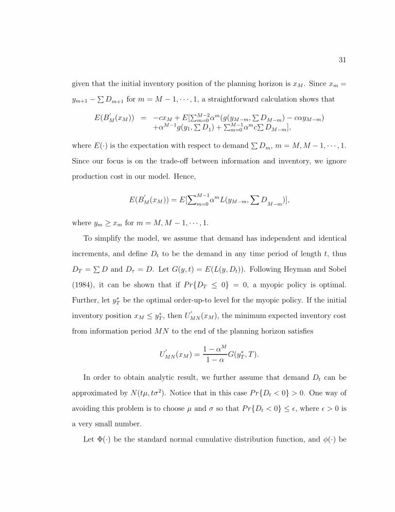
31

given that the initial inventory position of the planning horizon is xM . Since xm =

ym+1 −∑Dm+1 for m = M − 1, · · · , 1, a straightforward calculation shows that

E(B′M(xM )) = −cxM + E[

∑M−2m=0 αm(g(yM−m,

∑DM−m) − cαyM−m)

+αM−1g(y1,∑

D1) +∑M−1

m=0 αmc∑

DM−m],

where E(·) is the expectation with respect to demand∑

Dm, m = M, M − 1, · · · , 1.Since our focus is on the trade-off between information and inventory, we ignore

production cost in our model. Hence,

E(B′M(xM )) = E[

∑M−1

m=0αmL(yM−m,

∑D

M−m)],

where ym ≥ xm for m = M, M − 1, · · · , 1.To simplify the model, we assume that demand has independent and identical

increments, and define Dt to be the demand in any time period of length t, thus

DT =∑

D and Dτ = D. Let G(y, t) = E(L(y, Dt)). Following Heyman and Sobel

(1984), it can be shown that if Pr{DT ≤ 0} = 0, a myopic policy is optimal.

Further, let y∗T be the optimal order-up-to level for the myopic policy. If the initial

inventory position xM ≤ y∗T , then U

′MN(xM), the minimum expected inventory cost

from information period MN to the end of the planning horizon satisfies

U′MN(xM ) =

1 − αM

1 − αG(y∗

T , T ).

In order to obtain analytic result, we further assume that demand Dt can be

approximated by N(tμ, tσ2). Notice that in this case Pr{Dt < 0} > 0. One way of

avoiding this problem is to choose μ and σ so that Pr{Dt < 0} ≤ ε, where ε > 0 is

a very small number.

Let Φ(·) be the standard normal cumulative distribution function, and φ(·) be

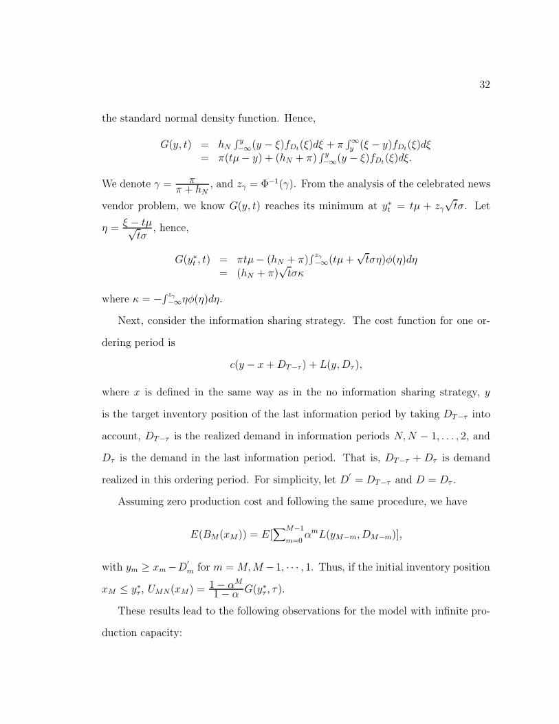
32

the standard normal density function. Hence,

G(y, t) = hN

∫ y−∞(y − ξ)fDt(ξ)dξ + π

∫∞y (ξ − y)fDt(ξ)dξ

= π(tμ− y) + (hN + π)∫ y−∞(y − ξ)fDt(ξ)dξ.

We denote γ = ππ + hN

, and zγ = Φ−1(γ). From the analysis of the celebrated news

vendor problem, we know G(y, t) reaches its minimum at y∗t = tμ + zγ

√tσ. Let

η =ξ − tμ√

tσ, hence,

G(y∗t , t) = πtμ− (hN + π)

∫ zγ−∞(tμ +

√tση)φ(η)dη

= (hN + π)√

tσκ

where κ = −∫ zγ−∞ηφ(η)dη.

Next, consider the information sharing strategy. The cost function for one or-

dering period is

c(y − x + DT−τ ) + L(y, Dτ ),

where x is defined in the same way as in the no information sharing strategy, y

is the target inventory position of the last information period by taking DT−τ into

account, DT−τ is the realized demand in information periods N, N − 1, . . . , 2, and

Dτ is the demand in the last information period. That is, DT−τ + Dτ is demand

realized in this ordering period. For simplicity, let D′= DT−τ and D = Dτ .

Assuming zero production cost and following the same procedure, we have

E(BM(xM)) = E[∑M−1

m=0αmL(yM−m, DM−m)],

with ym ≥ xm−D′m for m = M, M −1, · · · , 1. Thus, if the initial inventory position

xM ≤ y∗τ , UMN(xM) = 1 − αM

1 − α G(y∗τ , τ ).

These results lead to the following observations for the model with infinite pro-

duction capacity:

33

• Information sharing has the same fill rate as no information sharing.

• The expected cost in the information sharing strategy is proportional to√

τ

while expected cost under no information sharing is proportional to√

T =√

Nτ , where N is the number of information periods in one ordering period.

Thus, the percentage cost saving due to information sharing (defined as the

ratio between cost saving due to information sharing and the cost of no infor-

mation sharing) is proportional to 1 −√

(1/N),

• This implies that, if the initial inventory position is low so that we can reach

optimal order-up-to level, then 4 information periods will reduce total cost by

50% relative to no information sharing.

2.1.4 Analysis of non-dimensional parameters

Our objective in the analysis of non-dimensional parameters is to identify the param-

eters which may have an impact on the percentage cost reduction due to information

sharing. For simplicity, we focus on a single ordering period, but a similar method

can be applied to the problem with any number of ordering period.

Dividing both sides of Equation (1) by hNNμ, we get

U1(x)

hNNμ= min

xNμ

≤ yNμ

≤ xNμ

+ 1N

Cμ

{ c

hN

(y − x)

Nμ+

1

hNNμ

∫L(y, ξ)fD(ξ)dξ}

Let η = ξNμ, D

′= D

Nμ , it is easy to see that fD(ξ) = ddξ

FD(ξ) = ddξ

Pr( DNμ ≤

ξNμ) = d

dξFD′ (

ξNμ) = 1

NμfD′ (η). Hence,

1

hNNμ

∫L(y, ξ)fD(ξ)dξ =

∫((

y

Nμ− η)+ +

π

hN(η − y

Nμ)+

)fD′ (η)dη.

34

Let x′= x

Nμ , y′=

yNμ , c

′= c

hN, ρ =

μC , π

′= π

hN, U

′1 = U1

hNNμand L

′(y

′, η) =

(y′ − η)+ +π

′(η− y

′)+. We omit ′ from the notation without creating any confusion,

and we can rewrite the non-dimensionalized function U1 as follows:

U1(x) = minx≤y≤x+ 1

N1ρ

{c(y − x) +∫

L(y, η)fD(η)dη}.

A similar technique can be applied to Un(x) for n = 2, ..., N . Hence,

Un(x) = minx≤y≤x+ 1N

1ρ{c(y − x) +

hn−1

hN(y − x) + βEUn−1(y − D)},

n = N − 1, ..., 2

UN(x) = minx≤y≤x+ 1N

1ρ{c(y − x) +

hN−1

hN(y − x) + βEUN−1(y − D)} + x+

Thus, the percentage cost reduction associated with information sharing relative to

no information sharing depends only on the following non-dimensional parameters:

ρ, N , π, c, β and fD(η), where ρ is the capacity utilization μ/C , N is the frequency

of information sharing, π and c are the non-dimensionalized penalty and production

costs, and fD(η) is the probability density function of the non-dimensionalized de-

mand. In our computational study, we will focus on the impact of these parameters

on the benefit from information sharing.

2.1.5 Information sharing and the greedy policy

In this strategy, we apply a simple heuristics that makes production decisions so as

to match supply and demand. Such a greedy heuristic represents a special case of

the policies commonly used in practice. The reason that we study this policy is to

understand the benefits of using information optimally versus heuristically.

Specifically, the manufacturer produces in every information period, n = N −1, N − 2, . . . , 2 an amount equal to

min{C, Dn+1 − x−n },

35

where x−n = min{0, xn} is the shortage level at the beginning of the nth information

period. In the first information period, i.e., n = N , the manufacturer produces

min{C,−x−N}.

Finally, in the last information period, i.e., n = 1, the inventory level is raised to

a certain level determined by production capacity, inventory at the beginning of

the information period, production and inventory holding costs, and the demand

distribution. This can be done by solving a news vendor problem with capacity

constraint (please Lee and Nahmias 1993 for a review of news vendor problems).

2.2 Timing of information sharing

An important question in information sharing is when to share information? To

simplify the analysis, we focus on the single ordering period model and assume

that the retailer can share information with the manufacturer only once during the

ordering period. Intuitively, the higher the production capacity per unit time is, the

later the time information may be shared. Of course, the later time information is

shared, the more accurate the information on demand during the ordering period but

the smaller the remaining production capacity, i.e. the product of the per unit time

production capacity and the remaining time until the end of the ordering period.

For instance, if production capacity per unit of time is very high, information should

be transferred and used almost at the end of the ordering period. As production

capacity per unit of time decreases, we expect that it is optimal to share information

earlier. Thus, our objective is to find (1) the optimal time to share information, and

(2) the parameters which may affect the best timing for sharing information.

36

In order to find the optimal timing, we need to develop a continuous time model.

For this purpose, all notations associated with information period will be changed

to per unit of time, while the others remains the same. Hence, h is the inventory

holding cost per unit of time; C is the production capacity per unit of time; and D is

customer demand per unit of time with mean μ. Finally, we set β = 1 in this section

for simplification. Similar to the discrete time model, production is assumed to take

place at the full capacity rate C until the target inventory position is reached.

Consider an ordering interval [0, T ] and a given t < T , let T − t be the time

when information is shared. Thus, t = 0 (t = T ) implies that information is shared

at the end (beginning) of the ordering period. We assume that customer demand

Dτ in any time interval of length τ is Poisson(τμ). This implies that customer

demand at any time interval [t, t + τ ] ⊂ [0, T ] of length τ depends only on τ and

not on t, and demand in different time intervals (not overlapping) is independent.

The dynamic program is formulated below. Given that information is shared after

T − t units of time, let U1(x, t) (U2(x, t)) be the minimum expected inventory and

production costs from the time information is shared (the time the ordering period

starts, respectively) to the end of the horizon given an initial inventory position x.

U2(x, t) = minx≤y≤x+(T−t)C{c(y − x) + H2(x, y, t) + E(U1(y − DT−t, t))}U1(x, t) = minx≤y≤x+tC{c(y − x) + H1(x, y, t) + E(L(y, Dt))} (6)

where

H2(x, y, t) = T × h × x+ + h × t× (E(DT−t) − x) + h2

(y − x)2

C ,

H1(x, y, t) = h × t × x + h2

(y − x)2

C ,

L(y, D) = T × h × (y − D)+ + π × (D − y)+.

The first term of H2 represents the holding cost for initial inventory. The facts that

production line always runs at its full rate C , and the manufacturer will postpone

37

production as much as she can, explain the last term of H1, H2. The middle term

of H2 and the first term of H1 come from the fact that the inventory accumulated

in the first part of the ordering period (before information sharing) will be carried

throughout the second part of the ordering period. Assuming the initial inventory

position to be x and the order-up-to level in the first part to be y, then it equals

h×t×(y−x) = h×t×(y−DT−t+DT−t−x) = h×t×(y−DT−t)+h×t×(DT−t−x).

Take the expectation with respect to DT−t and notice that y − DT−t is the initial

inventory position at the beginning of the second part of the ordering period, then

we obtain the expression for H1, H2.

If t is fixed, then it is easy to show that V1(x, y, t) = c(y − x) + H1(x, y, t) +

E(L(y, Dt)) is jointly convex in both x and y (since the Hessians of H1(x, y, t),

H2(x, y, t) are positive semi-definite). This observation implies the following.

Proposition 2.2 U1(x, t) and U2(x, t) are convex in x.

Proof: : We start by proving that U1(x, t) is convex in x. Suppose we have x1, x2,

x1 �= x2, and y∗1, y

∗2, where U1(x1, t) = V1(x1, y

∗1 , t) with x1 ≤ y∗

1 ≤ x1 +(T − t)C and

U1(x2, t) = V1(x2, y∗2, t) with x2 ≤ y∗

2 ≤ x2 + (T − t)C . Let x = λx1 + (1 − λ)x2 and

y = λy∗1 + (1 − λ)y∗

2 , obviously, for any λ ∈ (0, 1), x ≤ y ≤ x + (T − t)C . Hence,

U1(x, t) = min{V1(x, y, t)|x ≤ y ≤ x + (T − t)C}≤ V1(x, y, t)≤ λV1(x1, y

∗1, t) + (1 − λ)V1(x2, y

∗2, t)

= λU1(x1, t) + (1 − λ)U1(x2, t).

To prove that U2(x, t) is convex, observe that since U1(x, t) is convex in x, thus

V2(x, y, t) = c(y − x) + H2(x, y, t) + E(U1(y −DT−t, t))

38

is jointly convex in x and y. Applying the same proof as before, we can show that

U2(x, t) is convex in x.

Unfortunately, it is not clear whether or not E(U1(y−DT−t, t)) and U2(x, t) are

convex in t. Thus, for any given t, we can compute the optimal y efficiently by using

Proposition 2.2. But to find the optimal timing of information sharing, we need to

discretize the ordering period and use enumeration.

We further analyze the impact of the timing of information sharing when the

retailer can transfer demand information to the manufacturer twice an ordering

period. Consider an ordering period [0, T ], let 0 ≤ t1 ≤ t2 ≤ T be the times when

information is shared, then the following dynamic program holds,

U3(x, t1, t2) = minx≤y≤x+t1C{c(y − x) + K3(x, y, t1) + E(U2(y − Dt1 , t1, t2))}U2(x, t1, t2) = minx≤y≤x+(t2−t1)C{c(y − x) + K2(x, y, t2) + E(U1(y − Dt2−t1 , t2))}

U1(x, t2) = minx≤y≤x+(T−t2)C{c(y − x) + K1(x, y) + E(L(y, DT−t2))},

where K3(x, y, t1) = T ×h×x+ + h2

(y − x)2

C + (T − t1)×h× (y−x), K2(x, y, t2) =

h2

(y − x)2

C + (T − t2) × h × (y − x), K1(x, y) = h2

(y − x)2

C . Similarly, we can show

U3(x, t1, t2), U2(x, t1, t2) and U1(x, t2) are convex in x. Since it is not clear whether

U3(x, t1, t2) is convex in t1, t2, we will compute the optimal timings by discretization

of the ordering period and enumeration.

Finally, we identify the non-dimensional parameters which may affect the optimal

timing. We divide Equation (6) by hT 2μ, let x′= x

Tμ , y′=

yTμ , t

′= t

T , c′= c

Th,

ρ = μC , π

′= π

Th, U

′1 = U1

hT 2μ, U

′2 = U2

hT 2μH

′1 = H1

hT 2μ, H

′2 = H2

hT 2μ, D

′= D

Tμ and

L′(y

′, η) = (y

′ − η)+ + π′(η − y

′)+. We omit ′ from the notation without creating

any confusion, and rewrite the non-dimensionalized functions U1(x, t) and U2(x, t)

39

as follows:

U2(x, t) = minx≤y≤x+

(1−t)ρ

{c(y − x) + H2(x, y, t) + E(U1(y − D1−t, t))}U1(x, t) = minx≤y≤x+ t

ρ{c(y − x) + H1(x, y, t) + E(L(y, Dt))}

where H2(x, y, t) = x+ + t(1− t− x) +ρ2(y − x)2, H1(x, y, t) = tx +

ρ2(y − x)2, and

L(y, D) = (y −D)+ + π(D − y)+. This analysis shows that the non-dimensional

optimal timing is a function of only ρ, π, c and fD(·), of which we will study the

effects of ρ and π in the following section.

In the case when information can be shared twice in one ordering period, a

similar non-dimensional analysis shows that the non-dimensional optimal timings

t1/T, t2/T are functions of only ρ, π, c and fD(·).

2.3 Computational results

In this Section, we use computational analysis to develop insights on the benefits

of information sharing. Our goal is two-fold: (1) determine situations where infor-

mation sharing provides significant cost savings compared to supply chains with no

information sharing; (2) identify the benefits of using information optimally com-

pared to using information greedily. Our focus is on the manufacturer’s cost and

service level.

According to Section 2.1.4, we examined cases with variations on the following

non-dimensional parameters: production capacity over mean demand, the number

of information periods in one ordering period, the time when information is shared,

coefficient of variation of demand distribution and finally the ratio between penalty

cost and inventory holding cost.

We set production cost equal to zero, and focus on holding and penalty costs.

40

Let inventory holding cost per ordering period to be equal to a constant 0.4 $

per unit product for all cases. Thus, the inventory holding cost per information

period is 0.4/N where N is the number of information periods within one ordering

period. Penalty cost varies from 1.9 to 7.9 $ per unit and takes the following values

1.9, 3.4, 4.9, 6.4, 7.9. In all cases of our computational analysis, the time discount

factor β is assume to be 1.

Let initial inventory at the beginning of the first ordering period, x, to be equal

to zero. To simplify the calculation, we use discrete probability distributions for

customer demand in one information period. In our study, we consider discrete

distributions such as Poisson, Uniform and Binomial. In addition, we also analyze

the following discrete distributions: the first, referred to as Disc1, demand takes

values from the set (0, 1, 3, 6) with probability (0.1, 0.3, 0.5, 0.1) respectively. In

the second, referred to as Disc2, demand takes the same values with probability

(0.05, 0.2, 0.7, 0.05), respectively.

The dynamic programming algorithms allow us to find the cost associated with

the first two strategies. For the third strategy, the newsboy model allows us to find

the optimal order-up-to level in the last information period of every ordering period,

while the cost associated with the strategy is estimated through simulation. Finally

simulation results provided us with service level for all three strategies. Following

convention, we measure service level by type one fill rate, which is defined to be the

expected fraction of ordering periods in which no backorders occur.

In the simulation models, each system is simulated 40, 000 times. The fill rate is

calculated as follows: let Xi be a random variable taking the value one if demand (at

the end of the ordering period) is satisfied with no shortage in the ith run, and zero

41

otherwise. Our estimation of the type one fill rate is the sample mean X =∑

i Xi/n,

where n is 40,000. Since our estimation of the standard deviation of Xi is equal to√X(1 − X), which is less than 0.5, thus, the length of a 95% confidence interval of

the fill rate is no more than 0.0098. Similarly, when we estimate the average cost for

the third strategy using simulation, we can ensure that a 95% confidence interval

has a length no larger than 0.098.

The following discussions are based on our computation results for models with

one ordering period and four information periods unless otherwise mentioned. For

multi-ordering period planning horizon, similar results are obtained.

2.3.1 The effect of information sharing on the optimal pol-

icy

Table 1: The impact of production capacity

demand distribution capacity/ED Penalty/Holding costs order-up-to-levelsPoisson(5) 1.2 8.5 (8,9,9,8)Poisson(5) 1.6 8.5 (2,5,7,8)Poisson(5) 2 8.5 (-4,1,5,8)

Uniform(0,1,...,9) 1.22 8.5 (10,10,10,8)Uniform(0,1,...,9) 1.67 8.5 (4,6,8,8)Uniform(0,1,...,9) 2.11 8.5 (-2,2,6,8)Binomial(0.5,10) 1.2 8.5 (6,7,7,7)Binomial(0.5,10) 1.6 8.5 (0,3,5,7)Binomial(0.5,10) 2 8.5 (-6,-1,3,7)

In this subsection we analyze the impact of capacity, penalty cost and demand

variability on the optimal policy when information is shared.

Table 1 presents the effect of production capacity for three different distributions

of demand in one information period. For each demand distribution, we increase

42

production capacity over average demand (the column capacity/ED) and calculate

the order-up-to-level in all information periods. Thus, the last column represents

the order-up-to-level for each of the four information periods.

Observe that

• Proposition 2.1 holds for almost all cases except the one for which capacity is

very tight, e.g., capacity/ED =1.2.

• As capacity increases, the difference between order up to levels in different

information periods increases. The intuition is clear: as capacity increases,

the optimal policy delays production as much as possible.

• The order-up-to-levels in the first few information periods may be negative,

which implies that the inventory position can be negative.

Table 2: The impact of penalty cost

Demand distribution capacity/ED Penalty/Holding costs order-up-to-levelsPoisson(5) 1.6 4.75 (0,3,6,7)Poisson(5) 1.6 12.25 (3,6,8,8)Poisson(5) 1.6 19.75 (5,7,9,9)

Uniform(0,1,...,9) 1.67 4.75 (1,4,7,8)Uniform(0,1,...,9) 1.67 12.25 (5,7,9,9)Uniform(0,1,...,9) 1.67 19.75 (7,8,9,9)Binomial(0.5,10) 1.6 4.75 (-1,2,5,6)Binomial(0.5,10) 1.6 12.25 (1,4,6,7)Binomial(0.5,10) 1.6 19.75 (2,4,6,8)

Table 2 analyzes the impact of penalty cost. In this table, we increase the ratio

of penalty to holding costs from 4.75 to 19.75 for each demand distribution. The

table demonstrates that

43

• As penalty cost increases, the order-up-to-level increases.

• As penalty cost increases, the difference between order up to levels in different

information periods decreases.

Table 3: The impact of demand variability

Demand distribution coefficient of variation order-up-to-levelsUniform(3,4,5,6) 0.25 (-3,1,4,6)Uniform(2,3,...,7) 0.38 (-1,2,5,7)Uniform(1,2,...,8) 0.51 (3,5,7,8)Uniform(0,1,...,9) 0.64 (7,8,9,9)

Table 3 presents the impact of demand variability. In this case the capacity over

average demand was kept constant, at a level of 1.67 for all cases, while penalty

over holding cost was 7.9 for all cases. It is easy to see the demand coefficient of

variation has a similar impact as the penalty cost. That is,

• As the coefficient of variation increases, the order-up-to-level increases.

• As the coefficient of variation increases, the difference between order up to

levels in different information periods decreases.

In Table 4 we consider two ordering periods with four information periods in

each one. We observe that the differences in the order-up-to-levels for the same

information periods between two consecutive ordering periods are small relative

to the average total demand in one ordering period. For example, in the case of

Binomial demand distribution, the maximal difference is 2 while the average total

demand in one ordering period is 20.

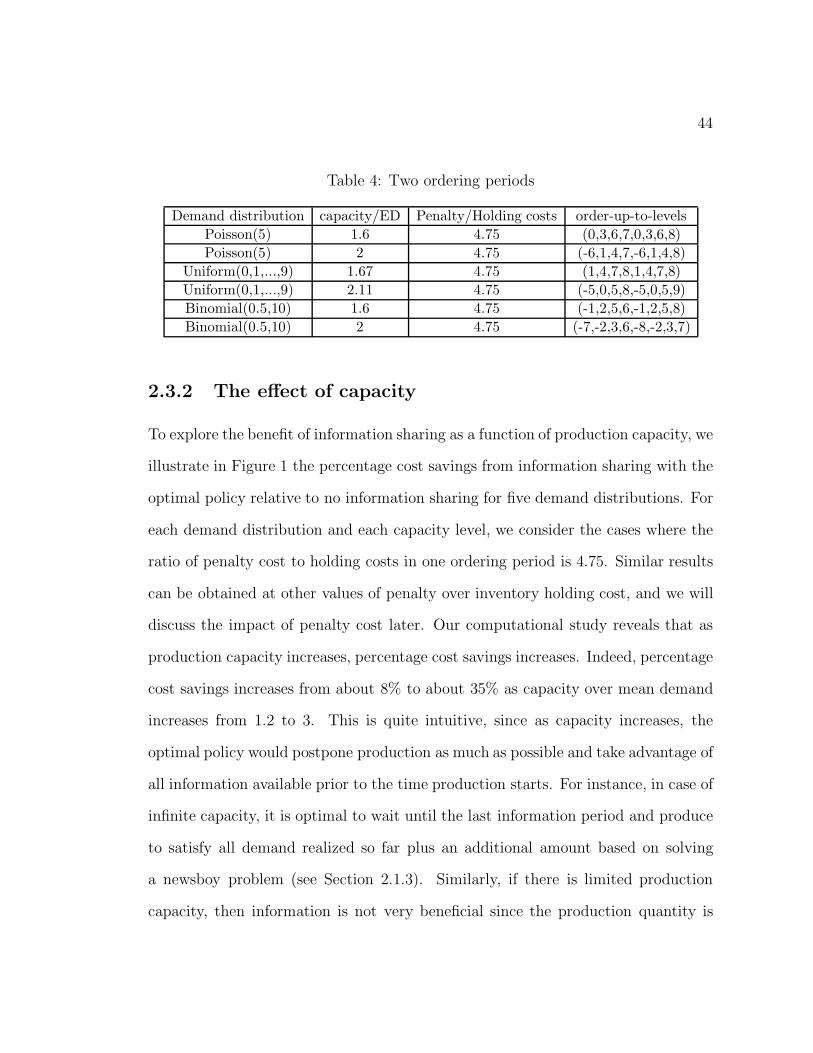
44

Table 4: Two ordering periods

Demand distribution capacity/ED Penalty/Holding costs order-up-to-levelsPoisson(5) 1.6 4.75 (0,3,6,7,0,3,6,8)Poisson(5) 2 4.75 (-6,1,4,7,-6,1,4,8)

Uniform(0,1,...,9) 1.67 4.75 (1,4,7,8,1,4,7,8)Uniform(0,1,...,9) 2.11 4.75 (-5,0,5,8,-5,0,5,9)Binomial(0.5,10) 1.6 4.75 (-1,2,5,6,-1,2,5,8)Binomial(0.5,10) 2 4.75 (-7,-2,3,6,-8,-2,3,7)

2.3.2 The effect of capacity

To explore the benefit of information sharing as a function of production capacity, we

illustrate in Figure 1 the percentage cost savings from information sharing with the

optimal policy relative to no information sharing for five demand distributions. For

each demand distribution and each capacity level, we consider the cases where the

ratio of penalty cost to holding costs in one ordering period is 4.75. Similar results

can be obtained at other values of penalty over inventory holding cost, and we will

discuss the impact of penalty cost later. Our computational study reveals that as

production capacity increases, percentage cost savings increases. Indeed, percentage

cost savings increases from about 8% to about 35% as capacity over mean demand

increases from 1.2 to 3. This is quite intuitive, since as capacity increases, the

optimal policy would postpone production as much as possible and take advantage of

all information available prior to the time production starts. For instance, in case of

infinite capacity, it is optimal to wait until the last information period and produce

to satisfy all demand realized so far plus an additional amount based on solving

a newsboy problem (see Section 2.1.3). Similarly, if there is limited production

capacity, then information is not very beneficial since the production quantity is

45

0

5

10

15

20

25

30

35

40

45

50

0 0.5 1 1.5 2 2.5 3 3.5

Capacity/Mean demand

% c

ost

sav

ing

Poisson(5)

Binomial(0.5,10)

Uniform(0,1,…,9)

Disc1

Disc2

Figure 1: The impact of production capacity.

mainly determined by capacity, not based on realized demand. Finally, from fill-

rate point of view, our computational study reveals that information sharing with

the optimal policy and the no information sharing strategies have almost identical

fill rates.

To explore the effectiveness of information sharing with the greedy policy, we

provide in Figure 2 the percentage cost savings of information sharing with the

optimal policy relative to information sharing with the greedy policy under similar

conditions as above. The Figure illustrates that

46

0

10

20

30

40

50

60

70

0 1 2 3 4 5Capacity/Mean demand

% c

ost

sav

ing

Disc1

Disc2

Possion(5)

Uniform(0,1,…,9)

Binomia(0.5,10)

Figure 2: The benefits of using information optimally.

• information sharing with the optimal policy reduces cost by at least 15% rel-

ative to information sharing with the greedy policy and the savings can be as

much as 50-60%.

• When capacity is tightly constrained, the savings provided by information

sharing with the optimal policy is relatively high. This is because the greedy

policy only responds to demand and does not build safety stock until the last

information period. In the last information period, if capacity is very tight,

the greedy policy may not be able to build as much safety stock as needed,

thus results in heavy penalty cost. On the other hand, the optimal policy can

47

-0.1

0

0.1

0.2

0.3

0.4

0.5

0.6

0.7

0.8

0.9

0 1 2 3 4 5

Capacity/Mean demand

Dif

fere

nce

of

typ

e o

ne

fill

rate

Disc1Disc2Possion(5)Uniform(0,1,…,9)Binomial(0.5,10)

Figure 3: Fill rates: the optimal policy vs. the greedy policy.

start building safety stock from the beginning of the ordering period by taking

advantage of excessive capacity in all information periods.

• As capacity increases, the benefit from information sharing with the optimal

policy relative to information sharing with the greedy policy decreases first and

then increases again. This is true, since as capacity becomes very large relative

to average demand, information sharing with the optimal policy will postpone

production as much as possible, while information sharing with the greedy

policy will build inventory starting from the beginning of ordering periods,

thus results in heavy inventory holding cost.

48

Figure 3 shows the difference between type-one fill rates for information sharing

with the optimal policy and information sharing with the greedy policy as a function

of production capacity for various demand distributions. The figure demonstrates

that when capacity is relatively tight, the difference in the fill-rates may be sub-

stantial. However, as capacity increases, the two strategies have almost identical

fill-rates.

2.3.3 The effect of penalty cost

To explore the benefit of information sharing as a function of the penalty cost, we

present in Figure 4 the percentage cost savings with information sharing relative

to no information sharing. The Figure illustrates the percentage cost savings as a

function of the ratio between penalty cost and inventory holding cost for various

capacity levels. Demand distribution in one information period is assumed to be

Uniform(0, 1, · · · , 9).The Figure 4 illustrates that

• When capacity is tightly constrained (e.g. capacity/mean demand =1.2), the

percentage cost saving could decrease as penalty cost increases. This is ex-

plained as follows: when capacity is tightly constrained, the total cost for both

the no information sharing and information sharing strategy increases quite

fast as penalty costs increases. Thus, the percentage saving decreases.

• When capacity is not tightly constrained, the benefit from information sharing

increases initially as penalty cost increases. As Kapuscinski and Tayur (1998)

points out, benefit from information sharing eventually decreases as penalty

cost becomes very large.

49

0

5

10

15

20

25

30

35

40

45

50

0 5 10 15 20 25Penalty/Holding cost

% c

ost

sav

ing Capacity/Mean

demand=32.11

1.67

1.22

Figure 4: The impact of penalty cost

2.3.4 The effect of the number of information periods

To explore the benefit of information sharing as a function of the number of informa-

tion periods, we present in Figures 5 the percentage cost savings with information

sharing relative to no information sharing for two production capacity levels. The

number of information periods, N , was 2,4,6 and 8 while the length of the ordering

period was assumed to be constant in all the models. The demand distribution

during the entire ordering period is assumed to be Poisson(λ) with λ = 24, hence

demand in a single information period follows Poisson(λ/N). Similarly, the total

production capacity, and the inventory holding cost per item, in the entire ordering

50

0

10

20

30

40

50

60

70

0 2 4 6 8 10Number of information period in one ordering

period

% c

ost

sav

ing

Capacity/meandemand = infinityCapacity/meandemand=2Capacity/meandemand=4/3

Figure 5: The impact of information sharing frequency.

period are kept constant and are equally divided among the different information

periods. The ratio of penalty to holding cost is 4.75. Figure 5 illustrates that

• As the number of information periods increases, the percentage savings in-

creases.

• Most of the benefits from information sharing is achieved within about 4 infor-

mation periods. That is, the marginal benefit is a decreasing function of the

number of information periods. Specifically, the benefit achieved by increasing

the number of information periods from 4 to 8 is relatively small.

51

0

0.1

0.2

0.3

0.4

0.5

0.6

0.7

0.8

0 0.2 0.4 0.6 0.8 1

Time when information is shared

Co

st

Capacity/Meandemand=1.67

2

3.3

5

Figure 6: The impact of the timing of information sharing.

• Define the maximum potential benefit from information sharing to be the per-

centage cost reduction when the manufacturer has unlimited capacity. A man-

ufacturer with production capacity twice as much as mean demand can achieve

a substantial percentage of the maximum potential benefit, e.g., when the fre-

quency of information period is 4, the manufacturer can obtain about 50% of

the cost benefit that a manufacturer with unlimited capacity can achieve.

2.3.5 Optimal timing for information sharing

In this subsection we analyze the impact of the time(s) when information is shared

on the manufacturer’s total inventory and penalty costs.

52

Sharing information once in one ordering period

Figure 6 presents the manufacturer’s total cost as a function of the time when

information is shared, assuming that the manufacturer can only share information

once in one ordering period. The Figure provides the normalized manufacturer’s

cost as a function of a normalized time. That is, time is normalized and is mea-

sured from 0 to 1, while the cost is normalized by the cost of carrying one ordering

period’s expected demand for one ordering period. Thus, 0 in x coordinate implies

that information is shared at the beginning of ordering period, and 1 means that

information is shared at the end of the ordering period and hence can not be uti-

lized. Demand distribution is assumed to be Poisson(10) and penalty over holding

cost equals 4.

In Figure 7 we study the impact of the production capacity and penalty cost on

the optimal timing of information sharing. These figures illustrate that

• As information sharing is delayed, the manufacturer’s total cost first decreases

and then increases sharply. The cost reaches its maximum when information

is shared at the beginning or end of one ordering period.

• The optimal timing for information sharing is not in the middle of ordering

period for any combination of production capacity and penalty cost, rather,

it’s in the later half of the ordering period.

• Both the production capacity and penalty cost have minor effects on the opti-

mal timing of information sharing. For all combination of production capacity

and penalty cost, the optimal timing is somewhere between 0.75 to 0.9 of

normalized time, and very close to 0.8 on average.

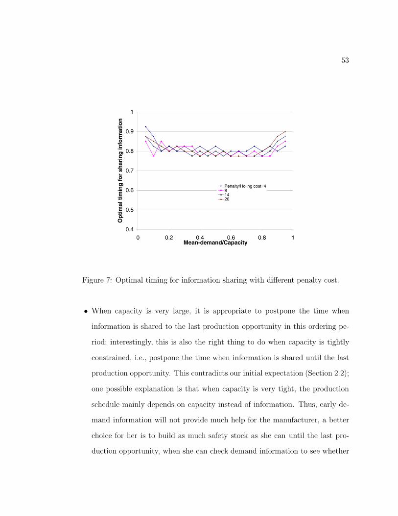
53

0.4

0.5

0.6

0.7

0.8

0.9

1

0 0.2 0.4 0.6 0.8 1Mean-demand/Capacity

Op

tim

al t

imin

g f

or

shar

ing

info

rmat

ion

Penalty/Holing cost=481420

Figure 7: Optimal timing for information sharing with different penalty cost.

• When capacity is very large, it is appropriate to postpone the time when

information is shared to the last production opportunity in this ordering pe-

riod; interestingly, this is also the right thing to do when capacity is tightly

constrained, i.e., postpone the time when information is shared until the last

production opportunity. This contradicts our initial expectation (Section 2.2);

one possible explanation is that when capacity is very tight, the production

schedule mainly depends on capacity instead of information. Thus, early de-

mand information will not provide much help for the manufacturer, a better

choice for her is to build as much safety stock as she can until the last pro-

duction opportunity, when she can check demand information to see whether

54

0

0.2

0.4

0.6

0.8

1

0

0.2

0.4

0.6

0.8

10

0.1

0.2

0.3

0.4

0.5

0.6

0.7

0.8

0.9

t1t2

Cos

t

Figure 8: The impact of the timing of information sharing.

she needs to produce more or not, before the demand is finally realized.

Sharing information twice in one ordering period

Figure 8 presents the manufacturer’s total cost as a function of the times when

information is shared, assuming that the manufacturer can share information twice

in one ordering period. Similar to the previous Section, the Figure provides the

normalized manufacturer’s cost as a function of a normalized time. Demand distri-

bution is assumed to be Poisson(10), penalty over holding cost equals 4, and the

production capacity is twice as much as the mean demand. Figure 9 illustrates the

manufacturer’s cost as a function of t1/T for given t2/T .

55

0.5

0.55

0.6

0.65

0.7

0.75

0.8

0.85

0 0.2 0.4 0.6 0.8 1 1.2

t1

Co

st

t2=1t2=0.9t2=0.8t2=0.6t2=0.4t2=0.2

Figure 9: The impact of the timing of information sharing.

In Figure 10 we study the impact of the production capacity and penalty cost

on the optimal timings of information sharing. The higher curves are the optimal

timing for the second information sharing, and the lower curves are the optimal

timing for the first information transferring. These figures illustrate that

• Sharing information twice an ordering period may help the manufacturer

achieve substantially more benefits than sharing information once, e.g. in Fig-

ure 9, the manufacturer’s maximum cost saving increases from 14.6% (once

an ordering period) to 20.7% (twice an ordering period).

• The optimal timing of the first information sharing varies significantly as the

56

0

0.2

0.4

0.6

0.8

1

1.2

0 0.2 0.4 0.6 0.8 1

Mean demand/capacity

Op

tim

al t

imin

gs

Penalty/Holding = 8, t28, t1

12, t2

12, t1

16, t2

16, t1

20, t2

20, t1

Figure 10: The impact of capacity and penalty cost on the optimal timing.

ratio between mean demand and production capacity changes, and it ap-

proaches the end of the ordering period as the ratio tends to zero. The ratio

between penalty and holding cost also has an impact on this optimal timing,

especially when capacity utilization is neither very high nor very low.

• The optimal timing of the second information sharing varies slightly for differ-

ent ratios between the mean demand and production capacity, and approaches

the end of the ordering period as the ratio tends to zero.

• The optimal timing of the second information transferring is unlikely to be

in the first half of the ordering period for all combination of parameters. On

57

the other hand, the optimal timing of the first information sharing can be

either in the first or the second halves of the ordering period. Indeed, in

our computational results the optimal timing of the first information sharing

varied from 0.22 to 0.82.

2.4 Conclusion

In this chapter, we consider a two-stage supply chain with a single retailer facing i.i.d

demand and a single manufacturer with finite production capacity. In the model, the

manufacturer receives demand information from retailer even during time periods

in which the retailer does not order. By analyzing the model in finite time horizon,

we study the value of information sharing for the manufacturer as well as how the

manufacturer can use the shared demand information effectively.

As for the optimal inventory control policy with information sharing, we find the

following property holds under certain conditions: the optimal order-up-to-levels in

any ordering period increase as we move from the first information period to the

last one. From our computational analysis, we find that even if these conditions do

not hold, the property is still true in most cases except when production capacity is

tightly constrained.

We demonstrate, through an extensive computational study, the potential ben-

efits of sharing demand information in terms of the manufacturer’s cost and service

level. For instance, if the manufacturer has a large capacity, information sharing

can be very beneficial. Indeed, the manufacturer can cut down inventory cost while

maintaining service level to the retailer by using information effectively. One in-

teresting observation is that the manufacturer can realize most of the benefits from

58

information sharing if the retailer shares demand information with the manufacturer

only a few times in each ordering period.

If the retailer has only one opportunity to share information with the manufac-

turer, then the best timing to share information is in the later half of the ordering

period. Parameters such as the production capacity and penalty cost have limited

impact on the optimal timing.

Finally, although the greedy policy is easy to implement, it may not perform

well in manufacturer’s costs and fill rate.

In this chapter we focus exclusively on the benefit of information sharing for the

manufacturer. In fact, information sharing can be also beneficial to the retailer if

the retailer and the manufacturer share the benefits. For example, the manufac-

turer can provide a better service level to the retailer in exchange for the demand

information. As we discuss in Section 2.1, this represents a very interesting future

research direction. Another future research direction is the impact of information

sharing on multi-product capacitated production systems in finite time horizon.

Chapter 3

A capacitated two-stage supplychain: infinite time horizon

In this chapter we extend the analysis of the previous chapter to the infinite time

horizon model. Specifically, we study the value of information sharing in a two-

stage supply chain with a single manufacturer and a single retailer in infinite time

horizon, where the manufacturer has finite production capacity and the retailer faces

independent demand. As before, the manufacturer receives demand information

even during periods of time in which the retailer does not order. Allowing for time

varying cost functions, our objective is to characterize the impact of information

sharing on the manufacturer’s cost and service level.

The optimal control of a periodic review production-inventory system in infinite

time horizon is a classical Markov decision problem with infinite state space and

unbounded cost function. The literature on these problems is quite voluminous, see

e.g., Heyman and Sobel (1984), Bertsekas (1987) and Puterman (1994) for general

theory of Markov decision process; Karlin (1960a, b), Zipkin (1989), Sethi and Cheng

(1997), and Song and Zipkin (1993) for systems with time varying parameters; and

59

60

Federgruen and Zipkin (1986a) and (1986b) for systems with production capacity

constraints.

The work of Aviv and Federgruen (1997) and Kapuscinski and Tayur (1998) is

closely related to our research. These authors analyzed periodic review production-

inventory systems with capacity constraints and time varying parameters. They

show that a modified cyclic order-up-to policy, i.e., a modified order-up-to policy

with periodically varying order-up-to levels, is optimal under both discounted and

average cost criterion. This is done by employing the optimality conditions devel-

oped by Sennott (1989) and Federgruen, Schweitzer and Tijms (1983).

In the next Section we describe our model and identify the main differences

between our model and results and those of Aviv and Federgruen (1997) and Ka-

puscinski and Tayur (1998).

3.1 The model

Consider the infinite time horizon version of the model analyzed in Chapter 2. In

this periodic review model, a single capacitated manufacturer can receive demand

information from a single retailer every τ units of time, while the retailer places

orders every T time periods, τ ≤ T . The external demand faced by the retailer

is assumed to be independent, but not necessarily identical, and the retailer uses

an order-up-to inventory policy to control her inventory. In what follows, we focus

on the differences between the model that we discuss here and the model that we

analyze in Chapter 2.

Let N = T/τ be an integer which represents the number of information periods

in one ordering period. We index information periods within one ordering period

61

1, 2, . . . , N where 1 is the first information period in the ordering period and N is the

last. We use Di to denote the end user demand in information period i, i = 1, . . . , N .

Di is assumed to be independent, its distribution only depends on i, and its mean is

defined as EDi. To simplify the analysis, we assume that costs do not change from

information period to information period; later we will demonstrate that our results

can be easily extended to include cases where costs change periodically within one

ordering period but are the same across different ordering periods.

We start by considering a finite time horizon model with M ordering periods.

Index the ordering periods from 0 to M − 1 where the 0 ordering period is the first

one and the M − 1 ordering period is the last one. The finite horizon starts in the

first ordering period at the beginning of the jth information period, 1 ≤ j ≤ N .

Consider the ith information period, i = 1, 2, . . . , N, in ordering period m, m =

0, 1, . . . , M − 1. Of course, mN + i ≥ j. We refer to this information period as the

mN + i information period. For instance, information period mN + 1 is the first

information period in the mth ordering cycle. We refer to this indexing convention

as a forward indexing process.

Define Si to be the state space for inventory position x at the beginning of

the ith information period, and y − x is the amount produced in that information

period, y ∈ Ax and Ax is the set of feasible actions. Let ξ(x, y, D) to be the transition

function and D be the demand. In our case, Ax = [x, x+C ], and ξ(x, y, D) = y−D.

It is easy to verify that gmN+i(x, y), i = 1, 2, . . . , N ,m = 0, . . . , M − 1, the

expected inventory and production cost in information period mN + i given that

the period starts with an inventory position x and produces in that period y − x

62

items, can be written as follows.

gmN+i(x, y) =

{c(y − x) + E(L(y, DN )), i = Nc(y − x) + hN−i(y − x), otherwise,

where E(·) is the expectation with respect to DN . Since gmN+i(x, y) depends only

on i and not m, we can write gmN+i(x, y) = ri(x, y), ∀m = 0, 1, . . . , M − 1 and all

i =, 1, . . . , N . Furthermore, ri(x, y) can be written as the sum of a function of x,

(φi(x)) and a function of y, (ϕi(y)) where

φi(x) =

{ −cx, i = N−(c + hN−i)x, otherwise,

ϕi(y) =

{cy + E(L(y, DN )), i = N(c + hN−i)y, otherwise,

and

L(y, D) = hN (y − D)+

+ π(D − y)+.

Finally, we assume the salvage cost function gMN+1 = 0.

We define the optimal policy under discounted cost criterion as follows. Let

σ = {σ1, σ2, . . .} be any feasible policy where σk is a function depending on the

initial inventory position in period k, i.e. σk = σk(x) and σk(x) ∈ Ax for all k. Let

Π be the set of all feasible policies. Define the expected discounted cost from the

ith information period in the first ordering period until the end of the horizon when

M → ∞, as

Uβi (x, σ) = E( lim

M→∞

MN∑k=i

βk−igk(xk, σk(xk))|xi = x),

where E(·) denotes the expectation with respect to demand in all information pe-

riods, and xi is the initial inventory position of the ith information period for

63

i = 1, 2, . . . , N . A policy σ∗ = {σ∗1, σ

∗2, . . .} ∈ Π is called optimal under the dis-

counted cost criterion if for all x ∈ S and i,

Uβi (x, σ∗) = inf

σ∈ΠUβ

i (x, σ).

To simplify the notation, we define uβi (x) = Uβ

i (x, σ∗).

Similarly, the optimal policy in infinite time horizon under average cost criterion

can be defined. Following Heyman and Sobel, the performance measure for any

feasible policy δ = {δ1, δ2, . . .} ∈ Π under average cost criterion is defined as follows,

Gi(x, δ) = limM→∞ sup(

E{MN∑k=i

gk(xk, δk(xk))|xi = x}MN − i + 1

).

As before, a policy δ∗ is optimal if it minimizes Gi(x, δ) for all x and i over Π.

It is easily seen that, in our model of information sharing, except for those pe-

riods in which orders are placed, the cost function ϕi(y) can go to negative infinity

as y → −∞. This implies that the results obtained by both Aviv and Federgruen

and Kapuscinski and Tayur cannot be applied to this model since they all assume

ϕi(y), for all i, are bounded from below. To further explain the difference between

this model and previous models, consider following three cases. First, if the manu-

facturer only has inventory holding cost but no penalty cost for all periods, then a

finite optimal policy does not exist, since producing nothing in all periods is clearly

the optimal policy. Second, if the manufacturer has both inventory holding cost

and penalty cost for all periods, then we have the models studied by Aviv and Fed-

ergruen (1997) and Kapuscinski and Tayur (1998). Finally, if in some periods the

manufacturer only has inventory holding cost, while in other periods, she has both

holding and penalty cost, then it is not clear whether there exists a finite optimal

policy if the manufacturer has finite production capacity.

64

Thus, the objective of this chapter is two fold: First, characterize the finite

optimal policy for the information sharing model under both discounted and average

cost criterion. Second, identify the conditions under which information sharing is

most beneficial, that is, characterize how frequently information should be shared

and when it should be shared so that the manufacturer can maximize the potential

benefits.

For this purpose, we first develop a new method in Section 3.2 to prove that the

steady-state average cost is finite for any finite cyclic order-up-to policy under certain

non-restrictive conditions. Then, in Section 3.3.1 we characterize the conditions for

cyclic order-up-to policy to be optimal under the discounted cost criterion, and

prove that a cyclic order-up-to policy is also optimal under average cost criterion

(Section 3.3.2). Next, extensive computational study is conducted in Section 3.4,

using the Infinitesimal Perturbation Analysis (IPA), to characterize the effects

of frequency and timing of information sharing. Finally, we conclude the chapter

with a discussion of our results and contributions in Section 3.5.

3.2 Properties of cyclic order-up-to policy

Consider the information sharing problem with the cost function ri(x, y) ∼ O(|x|ρ)+O(|y|ρ), where ρ is a positive integer. Define a cyclic order-up-to policy as a policy

with different order-up-to levels for different information periods, but these levels

are the same for the same information period in different ordering periods. That is,

the order up to level in information period mN + i is the same for all m but may

be different for different i, i = 1, 2, . . . , N .

65

In this section we study the Markov processes associated with any cyclic order-

up-to policy and identify conditions under which they are positive recurrent and have

finite steady-state average cost. The conditions are similar to those identified by

Aviv and Federgruen and Kapascinski and Tayur but the analysis is quite different.

Let Di, i = 1, · · · , N be the random variable representing demand in information

period mN + i for all m, demand is assumed to be discrete. Consider a cyclic order-

up-to policy with levels a1, a2, · · · , aN , and define the shortfall processes {smN+i, m =

0, 1, · · ·} for different i = 1, · · · , N as smN+i = ai−ymN+i, if we are in period mN + i

and ymN+i is the inventory position at the end of this period before demand is

realized. Hence the dynamics of shortfall are,

smN+i+1 =

⎧⎪⎨⎪⎩

(ai+1 − ai) + smN+i + Di − C, if (ai+1 − ai) + smN+i + Di > C,0, if 0 ≤ (ai+1 − ai) + smN+i + Di ≤ C,(ai+1 − ai) + smN+i + Di, if (ai+1 − ai) + smN+i + Di < 0.

Observe that the shortfall can be negative when initial inventory is higher than the

order-up-to level in this period. If excessive stock is returned when the inventory

position is higher than the order-up-to level, then the dynamics of shortfall processes

{srmN+i, m = 0, 1, · · ·} for i = 1, · · · , N is sr

mN+i+1 = (ai+1 − ai + srmN+i + Di −C)+.

We refer to this policy as an order-up-to policy with returns.

Aviv and Federgruen show that if (1) E(Dli) < ∞ for all positive integers l ≤ ρ+1

and i = 1, · · · , N , (2) E(∑N

i=1 Di) < NC, then for any finite order-up-to policy, the

shortfall process has a finite set of states such that it can be reached with finite

expected cost from any starting state. Kapascinski and Tayur prove that in steady

state, E(|xi|ρ), E(|si|ρ) are finite for order-up-to zero policy under similar conditions

as those proved by Aviv and Federgruen, namely (1) E(D2ρ+2i ) < ∞ for i = 1, · · · , N ,

(2) E(∑N

i=1 Di) < NC.

66

Using a new and simpler method based on Foster’s criterion and one of its

extension, we will prove that {xmN+i, m = 0, 1, · · ·} (defined to be the inventory

positions at the beginning of mN + ith information period), {ymN+i, m = 0, 1, · · ·}(inventory positions at the end of mN + ith information period before demand

realized) and {smN+i, m = 0, 1, · · ·} (shortfalls) generated by any finite cyclic order-

up-to policy give rise to Markov Chains with single irreducible and positive recurrent

class and finite steady-state average cost under the same condition as Aviv and

Federgruen; that is we require (1) E(Dli) < ∞ for all positive integer l ≤ ρ + 1 and

i = 1, · · · , N , and (2) E(∑N

i=1 Di) < NC.

Our method is to first show that single irreducible and positive recurrent class

and finite steady state average cost hold true for order-up-to a constant (zero) policy

under these conditions. We then extend the results to any finite order-up-to policy

with returns. Finally, we show that properties such as positive recurrence and finite

steady-state average cost can be transferred from a system using a cyclic order-up-to

policy with returns to a similar system without returns.

We begin our analysis by presenting new proofs for the positive recurrence and

finite steady-state average cost of order-up-to zero policy. To simplify the analysis,

let’s assume Pr(Di < 0) = 0, ∀i.

Proposition 3.1 Given an order-up-to zero policy, the inventory positions {xmN+i,

m = 0, 1, · · ·}, {ymN+i, m = 0, 1, · · ·} and the shortfall process {smN+i, m = 0, 1, · · ·}for i = 1, · · · , N , generate Discrete Time Markov Chains (DTMC) with single irre-

ducible and positive recurrent class if∑N

i=1 EDi < NC.

Proof: See Section 5.3 for details.

67

The proof that the steady-state average cost associated with an order-up-to zero

policy is finite is based on the following generalization of Foster’s criterion.

Lemma 3.1 A generalization of Foster’s Criterion Consider an irreducible

and aperiodic Markov chain {Xn, n = 0, 1, · · ·} with a single period cost function

r(·), which is continuous and bounded from below. Assume there exists a potential

function V (·) mapping the state space S to [0,∞), and a constant η such that

E{V (Xn+1) − V (Xn)|Xn = x} ≤ −r(x) + η, ∀x ∈ S.

Then given an initial state x0 with V (x0) < ∞, the Markov chain Xn has finite

steady-state average cost if Xn is positive recurrent.

Proof: See Section 5.3 for details.

This Lemma is a variation of the generalization of Foster’s criterion by Meyn

and Tweedie (1993) (see Theorem 14.0.1 (f-regularity)). As we will see later, our

generalization allows us to prove the following.

Lemma 3.2 Consider an order-up-to zero policy. If E((Di)k) < ∞ for all integer

0 ≤ k ≤ ρ + 1, ∀i and∑N

i=1 EDi < NC, then in steady state

(1) E(|si|ρ) < ∞, E(|xi|ρ) < ∞ and E(|yi|ρ) < ∞ for all i = 1, · · · , N ,

(2) for 0 < β < 1, E(∑∞

n=0 βn|yn|ρ) < ∞ and E(∑∞

n=0 βn|xn|ρ) < ∞ for any

initial inventory position x0 and initial information period i.

Proof: See Section 5.3 for details.

Proposition 3.1 and Lemma 3.2 can be extended to any finite cyclic order-up-to

policy with returns as follows,

68

Proposition 3.2 Consider any finite cyclic order-up-to policy with returns. If∑N

i=1

EDi < NC and E((Di)k) ≤ ∞ for any positive integer k ≤ ρ + 1 and ∀i, then

(1) each shortfall process {srmN+i, m = 0, 1, · · ·}, i = 1, · · · , N gives rise to a

Markov chain with single irreducible and positive recurrent class,

(2) E(|xri |ρ) < ∞ and E(|yr

i |ρ) < ∞ for all i,

(3) for 0 < β < 1, E(∑∞

n=0 βn|yrn|ρ) < ∞ and E(

∑∞n=0 βn|xr

n|ρ) < ∞ for any

initial finite inventory position xr0 and initial information period i.

Proof: Assume ai, i = 1, · · · , N, to be the order-up-to levels. We only need to

transform this policy to an order-up-to 0 policy, and then apply Proposition 3.1 and

Lemma 3.2.

Consider yrmN+i, the inventory positions at the end of period mN + i before

demand is realized. For simplicity, we drop subscript mN . The system dynamics is

yri+1 = min{yr

i −Di +C, ai+1} = ai+1 +(yri −ai+1−Di +C)−, where x− = min{0, x}.

Let z′i = yr

i − ai and D′i = Di + (ai+1 − ai), then z

′i+1 = (z

′i − D

′i + C)− and

∑Ni=1 D

′i =

∑Ni=1 Di < NC. For z

′i and D

′i, this is order-up-to zero policy, where

demand D′i can be negative, but bounded from below.

Notice that the shortfall processes associated with this order-up-to zero policy

have state space {0, 1, 2, · · ·} even if demand can be negative. Using similar proofs

as those of Proposition 3.1 and Lemma 3.2, we can show that the same results

hold for this order-up-to zero policy if there exists a positive constant di so that

Pr{Di < −di} = 0, ∀i = 1, 2, · · · , N .

We are ready to study the gap between the inventory position processes without

returns, ymN+i, and with returns, yrmN+i, assuming they start with the same initial

inventory level and face the same stream of demand.

69

Proposition 3.3 Consider two inventory systems with cyclic order-up-to levels a1,

..., aN , for N ≥ 2, one system without returns and the second one with returns. If

the two systems start with the same initial state x0 ≤ max{a1, · · · , an}, and face

the same stream of random demand, then the stochastic process {zmN+i = ymN+i −yr

mN+i, m = 0, 1, · · ·} has following properties for all i:

(1) zmN+i ≥ 0 for all m,

(2) zmN+i ≤ max{a1, · · · , aN} − min{a1, · · · , aN} for all m.

Proof: The proof is by induction. Clearly, z1 = 0. Consider period mN + i and

assume 0 ≤ zmN+i ≤ max{a1, · · · , aN} − min{a1, · · · , aN}. We distinguish between

the following two cases. In the first case, ai ≤ ai+1 and in the second case ai > ai+1.

ai ≤ ai+1: There are two sub cases to consider. (1) xmN+i+1 and xrmN+i+1 are

no larger than ai+1. In this case ymN+i+1 = min{xmN+i+1 + c, ai+1} and yrmN+i+1 =

min{xrmN+i+1 + c, ai+1} and hence

0 ≤ ymN+i+1 − yrmN+i+1 ≤ xmN+i+1 − xr

mN+i+1 = ymN+i − yrmN+i.

(2) xmN+i+1 > ai+1 ≥ xrmN+i+1. This can only occur if N > 2, and ai+1 <

max{a1, · · · , aN}. Clearly, ymN+i+1 = xmN+i+1 and yrmN+i+1 = min{xr

mN+i+1 +

c, ai+1} which implies that

0 ≤ ymN+i+1 − yrmN+i+1 ≤ xmN+i+1 − xr

mN+i+1 = ymN+i − yrmN+i.

ai > ai+1: In this case there are three possible sub cases. (1) xmN+i+1 and

xrmN+i+1 are no larger than ai+1. (2) xmN+i+1 > ai+1 ≥ xr

mN+i+1. (3) xmN+i+1

and xrmN+i+1 are larger than ai+1. The proof of the first two sub cases is identi-

cal to the proof in the previous case. Consider (3) and observe that in this case

70

ymN+i+1 = xmN+i+1 and yrmN+i+1 = ai+1 and hence

0 ≤ ymN+i+1 − yrmN+i+1 = xmN+i+1 − ai+1 ≤ max{a1, · · · , aN} − min{a1, · · · , aN}.

Remark: If x0 > max{a1, · · · , aN}, then the state space for {zmN+i, m = 0, 1, · · ·}is {0, 1, · · · , x0 − min{a1, · · · , aN}}, ∀i.

Lemma 3.3 Consider two arbitrary irreducible DTMCs {xn, n = 0, 1, · · ·} and {yn,

n = 0, 1, · · ·} starting with same initial state. If their difference process {zn =

xn − yn, n = 0, 1, · · ·} has finite state space Sz, and if xn is positive recurrent and

has certain finite steady-state moments, then yn is also positive recurrent and the

same steady state moments of yn are finite.

Proof: First, we show that positive recurrence is transferable from yn to xn. Define

Sx, Sy to be the state space for {xn, n = 0, 1, · · ·} and {yn, n = 0, 1, · · ·}. Assume yn

is positive recurrent, using contradiction, we assume xn is transient or non-recurrent

for all of its states. Since yn = xn − zn and y0 = x0, we have

Pr{yn = i|y0} = Pr{yn = i|x0}=

∑k∈Sz

Pr{xn = i + k, zn = k|x0}=

∑k∈Sz

Pr{zn = k|xn = i + k, x0}Pr{xn = i + k|x0}≤ ∑

k∈SzPr{xn = i + k|x0}.

Since Sz has only a finite number of states, and xn is transient or non-recurrent, so

Pr{yn = i|y0} → 0 as n → ∞ for i ∈ Sy. This contradicts to the assumption that

yn is positive recurrent (see Kulkarni pg 80 Theorem 3.4, and Kemeny, Snell and

Knapp 1966 pg 36 Proposition 1-61).

Second, assume yn has finite steady state moments E(|y|l) for 0 < l ≤ ρ, where

ρ is a positive integer. Consider

71

∑i∈Sx

|i|ρPr{xn = i|x0}=

∑i∈Sx

|i|ρ∑k∈SzPr{yn = i− k, zn = k|x0}

=∑

i∈Sx|i|ρ∑k∈Sz

Pr{zn = k|yn = i − k, y0}Pr{yn = i − k|y0}≤ ∑

k∈Sz

∑i∈Sx

|i− k + k|ρPr{yn = i − k|y0},

Taking the limit n → ∞ on both side, we obtain

E(|x|ρ) ≤ |Sz|(E(|y|ρ) + c1E(|y|ρ−1) + · · · + cρ) < ∞.

where c1, · · · , cρ are positive finite constants, and |Sz| is the size of the state space

for zn.

This Lemma is quite intuitive; it provides a method to simplify Markov chains

with infinite state space and complicated dynamics. A consequence of Lemma 3.3,

Proposition 3.3 and 3.2 is,

Proposition 3.4 Consider any finite cyclic order-up-to policy σ. If∑N

i=1 EDi <

NC, and E((Di)k) ≤ ∞ for all i and positive integers k such that k ≤ ρ + 1, then

(1) each shortfall process {smN+i, m = 0, 1, · · ·}, i = 1, · · · , N gives rise to a

Markov chain with single irreducible and positive recurrent class,

(2) E(|xi|ρ) < ∞ and E(|yi|ρ) < ∞ for all i.

(3) For 0 < β < 1, E(∑∞

n=0 βn|xn|ρ) < ∞ and E(∑∞

n=0 βn|yn|ρ) < ∞ for any

finite initial inventory position x0 and initial information period i.

(4) For 0 < β < 1, we have

Uβi (x, σ) = E( lim

M→∞

MN∑k=i

βk−igk(xk, σk(xk))|xi = x) < ∞.

The next step is to show that the long-run average cost convergences to a finite

value.

72

Proposition 3.5 Consider the information sharing model, if∑N

i=1 EDi < NC, and

E((Di)l) < ∞ for any positive integer l ≤ ρ + 1 and all i. Using any finite cyclic

order-up-to policy, we have

limM→∞

E{MN∑k=i

gk(xk, yk)|xi = x}MN − i + 1

converges to a finite value independent of initial period i and initial state x.

Proof: From Proposition 3.4, we have that in steady state∑N

i=1 E(ri(x, y)) < ∞ due

to the assumption that ri(x, y) ∼ O(|x|ρ) + O(|y|ρ). The proposition also implies

that the shortfall processes and thus the inventory positions before and after demand

arrives, ymN+i and xmN+i+1, give rise to Markov chains with single irreducible and

positive recurrent class. Without loss of generality, assume that the Markov chains

are ergodic (Kulkarni 1995, Theorem 3.16). Let the steady state distribution for

(x, y) in the ith information period be pi(x,y), where (x, y) ∈ Ωi (the feasible region of

(x, y)), then E(ri(x, y)) =∑

(x,y)∈Ωi pi(x,y)ri(x, y) must converge since the summation

is over at most countable number of positive values and it is bounded from above.

Finally, applying the Proposition 1-61 (arithmetic average) of Kemeny, Snell and

Knapp, the long-run average cost converges and equals to the steady state average

cost.

3.3 A Markov decision process

Our objective in this section is to discuss the discounted and average cost criterion

and present optimal policies for the information sharing model. For discounted cost

criterion, we will mainly follow the ideas of Heyman and Sobel; while for average

73

cost criterion, we will take the advantage of the special cost structure of the problem,

and develop a simple proof based on the idea of Blackwell optimal policy.

3.3.1 Discounted cost criterion

In this subsection, we present conditions for cyclic order-up-to policy to be optimal

under discounted cost criterion. These conditions are due to Heyman and Sobel

(1984) and Federgruen and Zipkin (1986b). Their variations are discussed in Aviv

and Federgruen (1997) or Kapuscinski and Tayur (1998).

It is well known that for infinite horizon problems, if single-period cost functions

are bounded from below, then the optimal cost function uβi (x) (see Section 3.1 for

definition) satisfies the following Bellman’s equation,

uβi (x) = minx≤y≤x+C{ri(x, y) + βE(uβ

i−1(y − Di))},

for i = 1, 2, . . . , N , where subscript 0 refers to N . A finite horizon dynamic pro-

gramming provides a successive approximation method to find the optimal policy

(Bertsekas 1987).

We index periods in a reverse order starting at the end of the planning horizon.

Let m = 0 be the last ordering period while m = M − 1 be the first ordering

period. We set i = N for the first information period and 1 for the last information

period in any ordering period. Thus, period mN + i represents the ith information

period in the m − 1th ordering period. Finally, let gmN+i(x, y) = ri(x, y) denote the

single period expected cost in this information period. We refer to this indexing as

backward index, and we will only use backward index in this subsection.

Let UβmN+i(x) be the minimum expected total costs if there are mN + i periods

remaining in the planning horizon, starting with an initial state x. Let the salvage

74

cost Uβ0 ≡ 0, and hence,

UβmN+i(x) = Miny∈Ax{gmN+i(x, y) + βE(Uβ

mN+i−1(y −Di))}= Miny∈Ax{ri(x, y) + βE(Uβ

mN+i−1(y − Di))}where E(·) is the expectation with respect to Di. Since ri(x, y) can be written as

the sum of a function of x, (φi(x)) and a function of y, (ϕi(y)) where

φi(x) =

{ −cx, i = 1−(c + hi−1)x, otherwise,

ϕi(y) =

{cy + E(L(y, D1)), i = 1(c + hi−1)y, otherwise,

Thus, the following recursion must hold.

UβmN+i(x) = φi(x) + V β

mN+i(x)

V βmN+i(x) = Minx≤y≤x+C{Jβ

mN+i(y)}Jβ

mN+i(y) = ϕi(y) + βE(UβmN+i−1(y − Di)).

(1)

Observe that in the very first information period (i.e., information period (M −1)N + N = MN) of the entire planning horizon, we have to add hNx+ to Uβ

MN(x)

to account for the holding cost of initial inventory.

The dynamic programming model has the following properties:

(a) Cost function ri(x, y) for each information period i = 1, · · · , N is positive

and convex in y. Thus, the following property, proved in Kapuscinski and Tayur

(1998), holds, UβmN+i(x) ≥ Uβ

(m−1)N+i(x) for any x, m = 1, · · · , M and i = 1, · · · , N .

(b) ri(x, y) = φi(x) + ϕi(y) for all i, and there exists a positive integer ρ so

that φi(x) ∼ O|x|ρ and ϕi(y) ∼ O|y|ρ. From Proposition 3.4, the total expected

discounted cost using cyclic order-up-to policy is finite if∑N

i=1 EDi < NC, and

E((Di)l) < ∞ for any positive integer l ≤ ρ + 1, ∀i. Which implies Uβ

mN+i(x)

converge point-wise to a finite value for any finite x and for all i (Heyman and Sobel

Theorem 8-13). Let Uβi (x) denote the convergence point of Uβ

mN+i(x).

75

(c) Obviously, Ax = [x, x + C ] is convex and finite for all x if we consider

denumerable state space. Thus, following the proof of Heyman and Sobel Theorem

8-14, we obtain,

Proposition 3.6 Uβi (x) satisfies the Bellman’s equation

Uβi (x) = Miny∈Ax{ri(x, y) + βE(Uβ

i−1(ξ(x, y, Di)))}

for i = 1, · · · , N , where subscript 0 refers to N .

The next property of the dynamic programming model is:

(d) JβmN+i(y) is convex in y, for all m, i.

The main difficulty in proving that an order-up-to policy is optimal is that the

function ϕi(y) maybe unbounded from both above and below for some time periods.

To overcome this difficulty, we need to aggregate N consecutive information periods

and identify conditions under which the cost function for all these periods tends to

positive infinity as action variables approach either positive or negative infinity.

For this purpose, we re-arrange Equation (1) to get,

UβmN+i(x) = Miny∈Ax{ri(x, y) + βE(Uβ

mN+i−1(y − Di))}= Miny∈Ax{φi(x) + ϕi(y) + βE(Uβ

mN+i−1(y − Di))}= φi(x) + miny∈Ax{Jβ

mN+i(y)}

where JβmN+i(y) = ϕi(y) + βE(Uβ

mN+i−1(y − Di)). Hence,

JβmN+i(y) = wi(y) + βE{Miny

′∈BiyJβ

mN+i−1(y′)}, ∀i

where Biy = [y − Di, y − Di + C ],

wi(y) =

{(1 − β)cy + (hi−1 − βhi−2)y + β(c + hi−2)EDi, i �= 1,(1 − β)cy + E(L(y, Di)) − βhN−1y + β(c + hN−1)EDi, i = 1.

76

Aggregate N consecutive information periods starting from the ith information

period in one ordering period until the (i + 1)th information period in the next

ordering period, where i = N −1, N −2, · · · , 1. When i = N , the aggregation starts

from the N th information period in one ordering period until the 1st information

period in the same ordering period. We use here a cyclic order so that all indices j

refer to the ith information period if j mod N = i. Define

Wi(yi) = wi(yi) + βE{Minyi−1∈Biyiwi−1(yi−1) + βE{Minyi−2∈Bi−1

yi−1wi−2(yi−2)

+ · · · + βE{Minyi−N+1∈Bi−N+2yi−N+2

wi−N+1(yi−N+1)} · · ·}},

which is the total cost in terms of yi for these N information periods. Following the

same analysis as in Chapter 5 Section 5.2, we find that if βi−1π > c+hi−1, Wi(y) →+∞ as |y| → +∞, for i = 1, 2, · · · , N . Finally, if βN−1π > c + hN−1, Wi(y) → +∞as |y| → +∞ for all i = 1, 2, · · · , N , and thus lim|y|→+∞JmN+i(y) → +∞ for all m

and i.

From these analysis, we have the following results,

Theorem 3.1 For Markov decision process defined in Equation (1), if

(a)∑N

i=1 EDi < NC, and E((Di)l) < +∞ for any positive integer l ≤ ρ + 1, ∀i,

(b) βN−1π > c + hN−1,

then

(1) Order-up-to policy is optimal for any m and i,

(2) Optimal order-up-to levels y∗mN+i are bounded as m → +∞,

(3) JmN+i(y) convergences to Ji(y) for all y, i, and every limit of y∗mN+i is a

minimal point for Ji(x).

(4) Cyclic order-up-to policy is optimal under discounted cost criterion.

77

Proof: Since JβmN+i(y) is a convex function of y, and lim|y|→+∞Jβ

mN+i(y) → +∞ for

all m and i, the order-up-to policy is optimal for all m and i. Since UβmN+i(x) is

bounded from above for any m and finite x, order-up-to levels are finite as m →+∞ because of (b) (see the proof of Theorem 2 in Aviv and Federgruen). Notice

that UβmN+i(x) is nondecreasing and converges to Uβ

i (x), which implies JβmN+i(y)

is nondecreasing and converges to, say Jβi (y), due to the Monotone Convergence

Theorem. Hence, (3) is true (see the proof of Theorem 2 in Aviv and Federgruen).

Finally, (1), (2) and (3) implies that cyclic order-up-to policy is optimal under the

discounted cost criterion.

For the capacitated inventory system in which ϕi(y), ∀i is unbounded from above,

but bounded from below, Aviv and Federgruen (1997) find that under certain condi-

tion, the optimal order-up-to levels under the discounted cost criterion are uniformly

bounded for all 0 < ε ≤ β < 1. Here we extend their result to the case where ϕi(y)

is unbounded from both above and below for some i.

Proposition 3.7 For the Markov decision process defined by Equation (1), if the

conditions of Theorem 3.1 are satisfied, then the optimal order-up-to levels y∗i , i =

1, 2, . . . , N under the discounted cost criterion are uniformly bounded both from above

and from below for any 0 < ε ≤ β < 1. Furthermore, the bounds are independent of

β.

Proof: see Section 5.3 for details.

As we shall see in the next subsection, this property allows us to extend the

optimality of cyclic order-up-to policy from discounted cost criterion to average cost

criterion in a simple way.

78

3.3.2 Average cost criterion

The following lemma applies the varnishing discount method to show sufficient con-

ditions for the optimality of cyclic order-up-to policy under average cost criterion.

Theorem 3.2 Consider the information sharing model and suppose:

(a) Cyclic order-up-to policy is optimal under the discounted cost criterion,

(b) For all 0 < ε ≤ β < 1, the optimal order-up-to levels under discounted cost

criterion are uniformly bounded both from above and from below,

(c) The long-run average cost of any finite cyclic order-up-to policy converges to

a finite value,

then cyclic order-up-to policy is optimal under the average cost criterion.

Proof: Consider a sequence of β1, β2, · · · , βj, · · · ↑ 1 as j → ∞. Since the optimal

order-up-to levels under the discounted cost criterion are uniformly bounded from

both above and below for all 0 < ε ≤ β < 1, there must exist an finite cyclic order-

up-to policy f and a subsequence jn → ∞, so that f is the optimal policy for all

Uβjni (x), ∀i = 1, 2, . . . , N .

Since we can show that for any finite cyclic order-up-to policy σ,

Gi(x, σ) = limM→∞

E{MN∑k=i

gk(xk, σk(xk))|xi = x}MN − i + 1

converges to a finite value which is independent of the initial period i and initial

state x (see Proposition 3.5), then by Tauberian Theory (Heyman and Sobel, pg

172),

Gi(x, f) = limβjn↑1(1 − βjn)Uβjni (x)

≤ limβj↑1sup((1 − βj)Uβj

i (x))≤ Gi(x, δ), ∀δ ∈ Π; x, i

79

The last inequality is justified by the Lemma A2 of Sennott (1989).

Finally, we combine Theorem 3.2, Theorem 3.1, Proposition 3.7 and 3.5, to get

Proposition 3.8 In the information sharing model, if

(a)∑N

i=1 EDi < NC, and E((Di)l) < +∞ for any positive integer l ≤ ρ + 1, ∀i,

(b) βN−1π > c + hN−1,

then cyclic order-up-to policy is optimal under the average cost criterion.

3.4 Computational results

In this section, we report on an extensive computational study conducted to de-

velop insights about the benefits of information sharing. Our goal is to determine

situations where information sharing provides significant cost savings compared to

supply chains with no information sharing. In what follows, we determine the opti-

mal order-up-to levels under average cost criterion.

We examine the cases with variation on the following parameters: production

capacity, the number of information periods in one ordering period, and the time

when information is shared. In all the numerical studies, we set the production

cost c = 0 and focus on holding and penalty costs. The inventory holding cost per

ordering period is set to be a constant 4 $ per unit product for all cases. Thus,

the inventory holding cost per information period is 4/N where N is the number

of information periods within one ordering period. Finally, the initial inventory

position, x, at the beginning of the first ordering period is set to be zero without

loss of generality.

80

3.4.1 Computational method

To compute the optimal order-up-to levels and cost, we apply the Infinitesimal

Perturbation Analysis (IPA) (Fu 1994 and Glasserman and Tayur 1995) for the

production-inventory systems analyzed in this chapter.

The Model with Information Sharing

For capacitated, multi-echelon production-inventory systems with linear ordering

cost, Glasserman and Tayur (1995) develop the estimators for the derivatives of cost

function with respect to order-up-to levels, and prove these estimators converge

to the correct value for the finite horizon problems and infinite horizon problems

under discounted and average cost criteria. Since our models are special cases of

their general systems, their convergence results apply to our models. More detailed

description of the sample path derivatives, method validation and simulation are

included in Section 5.4.

The Model with No Information Sharing

In the model with no information sharing, the retailer only places orders at the

end of each ordering period to the manufacturer without transferring demand infor-

mation anytime during the ordering period. Since the retailer uses an order-up-to

policy with constant order-up-to level, the order placed by the retailer is equal to

the total demand in one ordering period. Thus, we assume that the manufacturer

knows the demand distribution in one ordering period. To make this model compa-

rable to the model with information sharing, we assume that the manufacturer also

charges inventory holding cost per information period.

The model with no information sharing can be considered as a special case of

81

the information sharing model. Indeed, consider an instance of the model with

no information and construct an information sharing model in which demand in

every information period within an ordering period is exactly zero except in the

last information period. Demand in this information period equals total demand

during that ordering period. This information sharing model has the same dynamic

programming formulation as the model with no information sharing. Thus, the

dynamic program designed to solve the information sharing model can be applied

to solve the model in which information is not shared. Finally, cyclic order-up-to

policy is optimal for the model with no information sharing under both discounted

and average cost criterion.

To find the best order-up-to levels for the model with no information sharing, we

use the same computational method as in the model of information sharing. Please

see Section 5.5 for more details.

3.4.2 The effect of capacity

To explore the benefit of information sharing, we examine in Figure 11 the percent-

age cost savings from information sharing relative to no information sharing as a

function of the production capacity. The demand distribution of one information

period are Poisson(5), Uniform(0,10) and truncated Normal(5,4). Where truncated

Normal distribution is defined as follows: when the realization of the random vari-

able is negative, we set it to be zero. For each demand distribution and each capacity

level, we consider the cases where the ratio of penalty cost to holding costs in one

ordering period is 4.75, and there are 4 information periods in each ordering period.

The computational study reveals that as production capacity increases, the percent-

82

0

5

10

15

20

25

30

35

40

0 0.5 1 1.5 2 2.5 3 3.5

Capacity/Mean demand

% c

ost

sav

ing

s

Poisson(5)Normal(5,4)Uniform(0,10)

Figure 11: The impact of the production capacity

age cost saving increases. Indeed, percentage cost saving increases from about 5%

to about 35% as capacity over mean demand increases from 1.2 to 3. This is quite

intuitive, since as capacity increases, the optimal policy would postpone production

as much as possible and take advantage of all information available prior to the

time production starts. For instance, in case of infinite capacity, it is optimal to

wait until the last information period and produce to satisfy all demand realized

so far plus an additional amount based on solving a newsboy problem. Similarly,

if the production capacity is very limited, then information is not that beneficial

since production quantity is mainly determined by capacity, not based on realized

demand. Finally, from fill-rate point of views, our computational study reveals that

83

information sharing and no information sharing have almost identical fill rates.

3.4.3 The effect of frequency of information sharing

To understand the impact of information sharing frequency, we display in Figure 12

the percentage cost savings from information sharing as a function of the number

of information periods in one ordering period, for two production capacity levels.

The number of information periods, N , was 2,4,6 and 8 while the length of the

ordering period was assumed to be constant in all cases. The demand distribution

during the entire ordering period is assumed to be Poisson with parameter λ = 18,

hence demand in a single information period is Poisson with parameter λ/N . Total

production capacity and inventory holding cost per item in the entire ordering pe-

riod are kept constant and equally divided among the different information periods.

Finally, the ratio of penalty to holding costs is set to be 4.75. Figure 12 illustrates

that

• As the number of information periods increases, the percentage savings in-

crease.

• Most of the benefits from information sharing is achieved within a few infor-

mation periods, e.g., 4. That is, the marginal benefit is a decreasing function

of the number of information periods. Specifically, the benefit achieved by

increasing the number of information periods from 4 to 8 is relatively small.

• Define the maximum potential benefit from information sharing to be the

percentage cost reduction when the manufacturer has unlimited capacity, i.e.

capacity equals M (see Chapter 2, Section 2.1.3). A manufacturer with pro-

duction capacity twice as much as mean demand can achieve a substantial

84

0

10

20

30

40

50

60

70

0 1 2 3 4 5 6 7 8 9

Number of information period in one ordering period

% c

ost

sav

ing

s Capacity/Mean demand = MCapacity/Mean demand=2Capacity/Mean demand=4/3

Figure 12: The impact of the frequency of information sharing

percentage of the maximum potential benefit, e.g., when the frequency of in-

formation period is 4, the manufacturer can obtain almost 50% of the benefit

that a manufacturer with unlimited capacity can achieve.

3.4.4 Optimal timing for information sharing

In this subsection, we study the impact of the time when information is shared,

given that the retailer only shares demand information once with the manufacturer

in one ordering period. For this purpose, we equally divide one ordering period

into 10 intervals, and compute the total cost for the manufacturer when the retailer

shares demand information with her at one of these intervals. The sample path

85

0

0.1

0.2

0.3

0.4

0.5

0.6

0 0.2 0.4 0.6 0.8 1 1.2

Timing of information sharing

Co

st

1.6723.335

Figure 13: The impact of the timing of information sharing.

derivatives are computed in a similar way as in the model of information sharing.

More details can be found in Section 5.6.

Figure 13 presents the total cost of the manufacturer as a function of the time

when information is shared. The figure provides normalized cost as a function of

normalized time. That is, time is normalized and is measured from 0 to 1, while cost

is normalized by hN · N · ED. Thus, 0 in x coordinate implies that information is

shared at the beginning of ordering period, and 1 means that information is shared

at the end of the ordering period and hence can not be used. Demand distribution

is assumed to be Poisson(24) and the ratio of penalty to holding costs is 4. This

figure illustrates that

86

• As information sharing is delayed, manufacturer’s cost first decreases and then

increases sharply. Cost reaches its maximum when information is shared at

the beginning or end of one ordering period.

• When capacity is very large relative to mean demand, e.g. capacity over

mean demand equals 5, it is appropriate to postpone the time of information

sharing to the last production opportunity in this ordering period, e.g., 0.9 of

one ordering period. On the other hand, when capacity is relatively tightly

constrained, i.e., capacity over mean demand = 2, 1.67, manufacturer’s cost is

less sensitive to the timing of information sharing. For instance, in these two

cases, cost keeps almost constant when the time of information sharing varies

from 0.4 to 0.9.

3.5 Conclusion

In this chapter, we analyzed the value of information sharing in a two-stage supply

chain with a single manufacturer and a single retailer. The manufacturer has finite

production capacity and she receives demand information from the retailer even

during periods of time in which the retailer does not make ordering decisions. We

prove that cyclic order-up-to policy is optimal under both discounted and average

cost criterion.

For this purpose, we show that for any finite cyclic order-up-to policy, the as-

sociated inventory positions and shortfalls give rise to Markov chains with single

irreducible, positive recurrent class and finite steady-state average cost under cer-

tain non-restrictive conditions. The proof is based on an extension of the Foster’s

criterion. Then, we prove that cyclic order-up-to policy is optimal under average

87

cost criterion by showing that the optimal order-up-to levels under discounted cost

criterion are uniformly bounded for 0 < ε < β < 1.

Using extensive computational study, we demonstrate the potential benefits of

information sharing on the manufacturer’s cost and service level. For instance, by

using information effectively, the manufacturer can cut down inventory cost by 5-

35% while maintaining or increasing service level to the retailer. One interesting

observation is that the manufacturer can realize most of the benefits from informa-

tion sharing if the retailer shares demand information with the manufacturer only

a few times in each ordering period.

Finally, we analyze the optimal timing of information sharing. We show that if

the retailer has only one opportunity to share information with the manufacturer in

one ordering period, then the best timing for sharing information is in the later half of

the ordering period. This is true when capacity is large relative to average demand.

On the other hand, when capacity is tightly constrained, the manufacturer’s cost

becomes less sensitive to the time when information is shared.

Chapter 4

A multi-stage supply chain:forecast accuracy

In this chapter, we consider a single product distribution system with a single man-

ufacturer, a single distribution center and multiple retailers in infinite time horizon.

The retailers place orders periodically and use order-up-to policy to control their

inventory. The distribution center serves as a cross docking point and transfers the

aggregated orders from the retailers to the manufacturer. Assuming stationary and

correlated external demands, we analyze the following two cases: In the first case,

which we refer to as no information sharing, the manufacturer only receives the ag-

gregated orders from the distribution center. In the second case, which we refer to as

information sharing, the manufacturer not only receives the aggregated orders, but

also the order and demand information of individual retailers. The objective of this

chapter is to understand the impact of information sharing on the manufacturer’s

forecast accuracy.

Recently, a number of papers have explored the benefits of information sharing

in distribution systems facing stationary and correlated demand. The results are

mixed. As we reviewed in Chapter 1, Lee, So and Tang (2000) show that sharing

88

89

the retailer’s demand information will bring substantial benefits for the manufac-

turer, and the benefits increase along with demand correlation. On the other hand,

Raghunathan (2001) shows that by intelligently analyzing the order history, the

manufacturer can retrieve all the demand information, and thus sharing informa-

tion provides no benefit to the manufacturer when external demand is stationary.

Both works focus on a system with a single manufacturer and a single retailer.

Of course, in practice, distribution systems often have multiple retailers, and

the aggregated order of all retailers generally cannot be decomposed into orders

of individual retailers. Thus, the manufacturer cannot retrieve the exact demand

information of all retailers by analyzing the aggregated order history. This raises an

important question: Can individual retailer’s demand and order information help

the manufacturer improve its forecast of future aggregated orders received from the

DCs?

To answer this question, we consider a general distribution system with a single

manufacturer, a single distribution center and multiple retailers facing correlated

external demand. Our objective is to quantify the impact of sharing demand and

order information of each individual retailers on the manufacturer’s forecast accu-

racy. We choose to focus on forecast accuracy instead of inventory cost since forecast

accuracy is directly related to inventory cost. As Aviv (2001) points out, inventory

cost is almost proportional to the forecast error. Thus, reducing forecast error is as

important as reducing demand variation.

As far as we are aware of, Aviv (2002) is the only work on forecast accuracy

involving a single supplier, multi-retailer system with correlated demand. The fo-

cus is on the value of sharing market signals, i.e., unexpected random events such

90

as promotions, part of which maybe observable by different parties, between the

supplier and the retailers.

This chapter is organized as follows: we describe the model in detail in Section

4.1, analyze the information sharing model in Section 4.2 and the no information

sharing model in Section 4.3. In Section 4.4, we present results from our numerical

study. The chapter is concluded in Section 4.5.

4.1 The model

Consider a supply chain with a single manufacturer receiving orders from a single

distribution center (DC). The DC serves a set I of non-identical retailers. The

retailers review their inventory status periodically, and place orders according to

an order-up-to inventory policy. The DC does not hold inventory, but serves as

a cross-docking point between the manufacturer and the retailers. Transportation

lead-time, L, between the DC and the manufacturer is assumed to be constant.

Since in practice DCs are often close to retailers, we assume that the transportation

lead-time between the DC and the retailers is negligible.

Define the time between two consecutive orders to be ordering period. We assume

that all the retailers have the same ordering period and order at the same time

interval. Without loss of generality, we assume that the transportation lead time L

is an integer multiple of an ordering period. Following Lee, So and Tang, we assume

that the retailers can return excess inventory for free, and all unsatisfied demand at

the retailers are backlogged. Throughout this chapter, we assume no communication

among the manufacturer, DC and the retailers within any ordering period, thus the

manufacturer cannot update its forecast during any ordering period.

91

Define the discrete times at which the retailers place orders to be tn, and the

external demand faced by retailer i ∈ I in the nth ordering period (between tn and

tn+1) to be Din. At the beginning of the n + 1th ordering period, tn+1, demand

Din is realized, the retailer makes a forecast F R,i

n+1 for future demands and places an

order qin+1 to the DC. Upon receiving the orders, the DC transfers the aggregated

order Qn+1 =∑

i∈I qin+1 to the manufacturer. At tn+1, the manufacturer receives

the order Qn+1 from the DC in no time and fills the order from on-hand inventory.

If the manufacturer cannot satisfy the entire order, then the DC can receive the

missing part from an alternative source (we point out that the same assumption is

made by Lee, So and Tang). Finally, the manufacturer makes a forecast F Mn+1 for

the aggregated retailers’ order, Qn+2, in next time period.

Our objective is to analyze the benefits of sharing demand information of indi-

vidual retailers to the manufacturer in infinite time horizon, assuming that external

demands at all retailers follow stationary, but retailer dependent, processes.

Notice that in order to satisfy the DC order, Qn+1 at tn+1, the manufacturer

has to make a forecast F Mn at time tn. The manufacturer’s ability of matching

demand with supply is determined by how good the forecast F Mn is compared to

Qn+1. We realize that the manufacturer may need to forecast the quantity Qn+1

well in advance because of production capacity constraints. Here we choose to focus

exclusively on the most updated forecast F Mn . Since no information is transferred

during an ordering period, one key problem the manufacturer facing at tn is that

she has to forecast the DC’s order (the aggregated retailers’ orders) at tn+1 without

knowing the demand Din during the nth time period. This demand information is

critical for the retailers to determine their orders qin+1 and hence Qn+1 =

∑i∈I qi

n+1 at

92

tn+1. Thus, even the most effective utilization of the demand and order information

at each individual store will not enable the manufacturer to forecast the future

orders from the retailers without error.

To simply the analysis, we assume that the demand faced by the ith ∈ I retailer

follows an AR(1) process with parameters ai, ρi and δi, i ∈ I as is assumed in the

papers of Lee, Padmanabhan and Whang (1997a, b) and Chen, Drezner, Ryan

and Simchi-Levi (1999). Lee, So and Tang (2001) point out that demand is often

positively correlated in time, thus, we assume that ρi ≥ 0, ∀i ∈ I . Finally, the

external demands are independent across different retailers.

Focus on the ith retailer, and omit the index i without causing any confusion.

Dn+1 = a + ρDn + εn+1,

where εn+1 ∼ N(0, δ2) are i.i.d Normal random variables, and a, ρ, δ are positive

constants. It’s easy to show that E(D) = a1 − ρ and V ar(D) = δ2

1 − ρ2 . Under

the infinite time horizon assumption, the retailer must know exactly the demand

process (see also Lee, So and Tang for a similar assumption). Thus, at time tn+1

the retailer knows the last period demand, Dn, and has to forecast the demand for

the time interval [tn+1, tn+1+L] to cover for transportation lead time. The retailer’s

forecast for period n + 1 + l, l = 0, . . . , L made at time tn+1 is

D′n+1+l = a(1 + ρ + · · · + ρl) + ρl+1Dn.

The retailer has to plan for the next L + 1 periods, and the forecast of the retailer

at time tn+1 of total demand in next L + 1 periods is

F Rn+1 = D

′n+1 + · · · + D

′n+1+L.

93

Since the retailer uses a myopic inventory policy, her order up to level is

yRn+1 = F R

n+1 + sR,

where sR is the retailer’s safety stock, which depends on the demand uncertainty,

lead time and the service level provided to external demand by the retailer.

Assuming that sR does not vary from period to period, the retailer can return

excessive stock at no cost, and noticing that all unsatisfied demand at the retailer

are backlogged, thus the retailer’s order quantity at time tn+1 is

qn+1 = F Rn+1 − F R

n + Dn

= (Dn − Dn−1)(ρ + ρ2 + · · · + ρL+1) + Dn

= (b + 1)Dn − bDn−1

= a(b + 1) + (bρ + ρ − b)Dn−1 + (b + 1)εn

= a + ρqn + (b + 1)εn − bεn−1,

(1)

where b = ρ + ρ2 + · · ·+ ρL+1 = ρ1 − ρL+1

1 − ρ . The mean of qn+1 is equal to E(D),

while the variance of qn+1 equals σ2 = V ar(D)(1 + 2b(b + 1)(1 − ρ)).

Thus, the aggregated order Qn+1 can be written as,

Qn+1 =∑

i∈I qin+1 =

∑i∈I ai(bi + 1) +

∑i∈I(biρi + ρi − bi)D

in−1 +

∑i∈I(bi + 1)εi

n

=∑

i∈I ai +∑

i∈I ρiqin +

∑i∈I(bi + 1)εi

n −∑i∈I biε

in−1.

We now analyze the manufacturer’s forecast. At time tn, the manufacturer

needs to make a forecast F Mn of the next DC’s order, Qn+1. We consider two sys-

tems depending on whether the manufacturer receives demand information from the

retailers. In the case of no information sharing, the manufacturer only receives the

aggregated orders from the DC. In the case of information sharing, the manufacturer

not only receives the aggregated orders from the DC, but also shares the order and

demand information of individual retailers.

94

4.2 Information sharing

Under information sharing, the manufacturer knows the values of ai, ρi, for each

i ∈ I and the exact level of demand up-to the demand at the beginning of period

tn, Din−1. Thus, the following Proposition holds

Proposition 4.1 Under information sharing, the minimum Mean Square Error

(MSE) forecast that the manufacturer can make at time tn, for the aggregated de-

mand Qn+1, is

FMn =

∑i∈I

ai(bi + 1) +∑i∈I

(biρi + ρi − bi)Din−1,

with a mean square error equal to

E((Qn+1 − FMn )2) = V ar(Qn+1 − F

Mn ) =

∑i∈I

(bi + 1)2δ2i .

Proof: To show that FM

n is the minimum MSE forecast that the manufacturer can

make at tn, consider any forecast F Mn ,

E((Qn+1 − F Mn )2) = V ar(Qn+1 − F M

n ) + E2(Qn+1 − F Mn )

≥ V ar(Qn+1 − F Mn )

= V ar(∑

i∈I(biρi + ρi − bi)Din−1 − F M

n ) +∑

i∈I(bi + 1)2δ2i .

The second equality comes from the fact that εin is independent of F M

n . This is true,

since F Mn depends only on historical data and not on εi

n.

Finally, it is easily seen that the FM

n is an unbiased estimator of Qn+1, and hence

E((Qn+1 − FMn )2) = V ar(Qn+1 − F

Mn ).

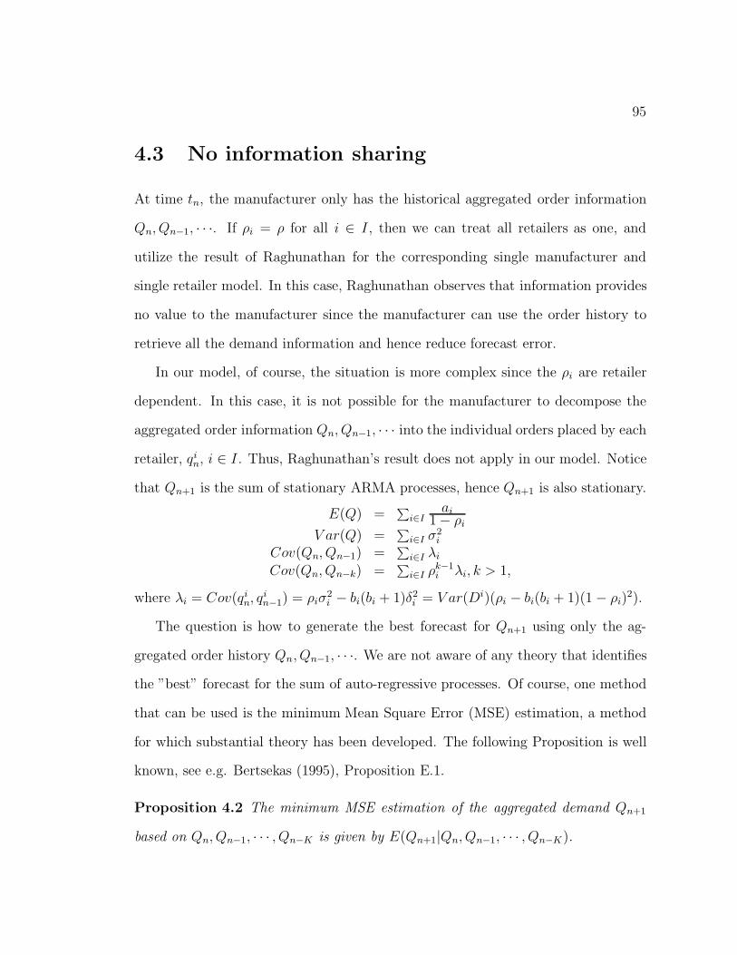
95

4.3 No information sharing

At time tn, the manufacturer only has the historical aggregated order information

Qn, Qn−1, · · ·. If ρi = ρ for all i ∈ I , then we can treat all retailers as one, and

utilize the result of Raghunathan for the corresponding single manufacturer and

single retailer model. In this case, Raghunathan observes that information provides

no value to the manufacturer since the manufacturer can use the order history to

retrieve all the demand information and hence reduce forecast error.

In our model, of course, the situation is more complex since the ρi are retailer

dependent. In this case, it is not possible for the manufacturer to decompose the

aggregated order information Qn, Qn−1, · · · into the individual orders placed by each

retailer, qin, i ∈ I . Thus, Raghunathan’s result does not apply in our model. Notice

that Qn+1 is the sum of stationary ARMA processes, hence Qn+1 is also stationary.

E(Q) =∑

i∈Iai

1 − ρi

V ar(Q) =∑

i∈I σ2i

Cov(Qn, Qn−1) =∑

i∈I λi

Cov(Qn, Qn−k) =∑

i∈I ρk−1i λi, k > 1,

where λi = Cov(qin, q

in−1) = ρiσ

2i − bi(bi + 1)δ2

i = V ar(Di)(ρi − bi(bi + 1)(1 − ρi)2).

The question is how to generate the best forecast for Qn+1 using only the ag-

gregated order history Qn, Qn−1, · · ·. We are not aware of any theory that identifies

the ”best” forecast for the sum of auto-regressive processes. Of course, one method

that can be used is the minimum Mean Square Error (MSE) estimation, a method

for which substantial theory has been developed. The following Proposition is well

known, see e.g. Bertsekas (1995), Proposition E.1.

Proposition 4.2 The minimum MSE estimation of the aggregated demand Qn+1

based on Qn, Qn−1, · · · , Qn−K is given by E(Qn+1|Qn, Qn−1, · · · , Qn−K).

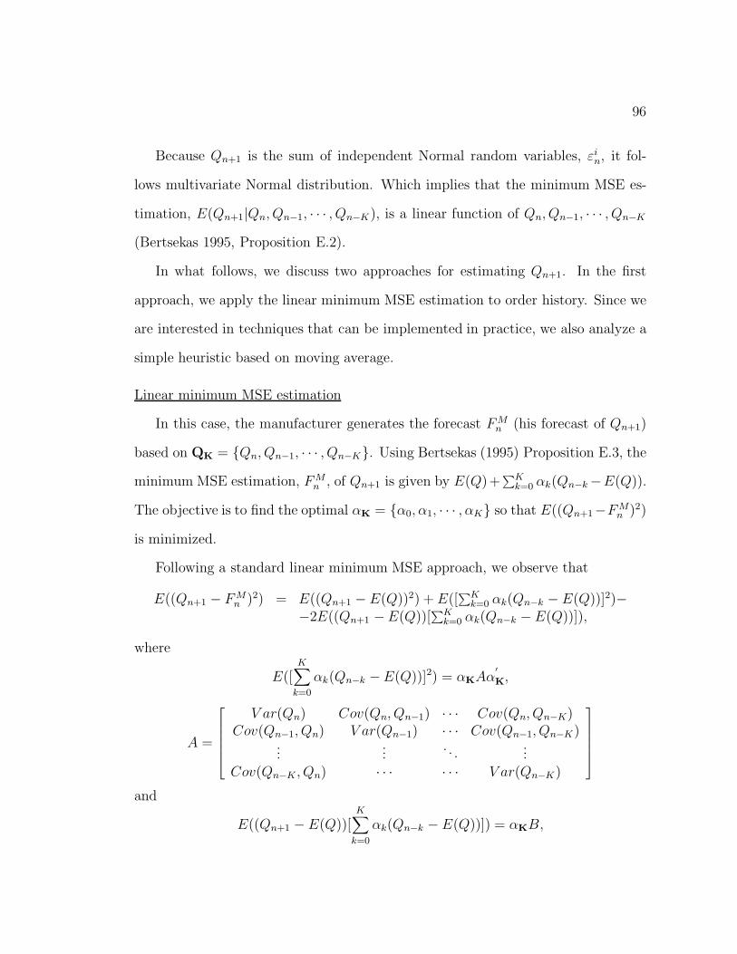
96

Because Qn+1 is the sum of independent Normal random variables, εin, it fol-

lows multivariate Normal distribution. Which implies that the minimum MSE es-

timation, E(Qn+1|Qn, Qn−1, · · · , Qn−K), is a linear function of Qn, Qn−1, · · · , Qn−K

(Bertsekas 1995, Proposition E.2).

In what follows, we discuss two approaches for estimating Qn+1. In the first

approach, we apply the linear minimum MSE estimation to order history. Since we

are interested in techniques that can be implemented in practice, we also analyze a

simple heuristic based on moving average.

Linear minimum MSE estimation

In this case, the manufacturer generates the forecast F Mn (his forecast of Qn+1)

based on QK = {Qn, Qn−1, · · · , Qn−K}. Using Bertsekas (1995) Proposition E.3, the

minimum MSE estimation, F Mn , of Qn+1 is given by E(Q)+

∑Kk=0 αk(Qn−k −E(Q)).

The objective is to find the optimal αK = {α0, α1, · · · , αK} so that E((Qn+1−F Mn )2)

is minimized.

Following a standard linear minimum MSE approach, we observe that

E((Qn+1 − F Mn )2) = E((Qn+1 − E(Q))2) + E([

∑Kk=0 αk(Qn−k − E(Q))]2)−

−2E((Qn+1 −E(Q))[∑K

k=0 αk(Qn−k − E(Q))]),

where

E([K∑

k=0

αk(Qn−k −E(Q))]2) = αKAα′K,

A =

⎡⎢⎢⎢⎢⎣

V ar(Qn) Cov(Qn, Qn−1) · · · Cov(Qn, Qn−K)Cov(Qn−1, Qn) V ar(Qn−1) · · · Cov(Qn−1, Qn−K)

......

. . ....

Cov(Qn−K , Qn) · · · · · · V ar(Qn−K)

⎤⎥⎥⎥⎥⎦

and

E((Qn+1 − E(Q))[K∑

k=0

αk(Qn−k − E(Q))]) = αKB,

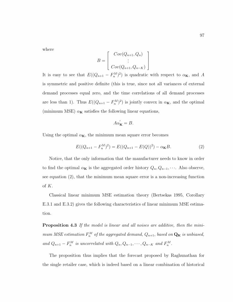
97

where

B =

⎡⎢⎢⎣

Cov(Qn+1, Qn)...

Cov(Qn+1, Qn−K)

⎤⎥⎥⎦

It is easy to see that E((Qn+1 − F Mn )2) is quadratic with respect to αK, and A

is symmetric and positive definite (this is true, since not all variances of external

demand processes equal zero, and the time correlations of all demand processes

are less than 1). Thus E((Qn+1 − F Mn )2) is jointly convex in αK, and the optimal

(minimum MSE) αK satisfies the following linear equations,

Aα′K = B.

Using the optimal αK, the minimum mean square error becomes

E((Qn+1 − F Mn )2) = E((Qn+1 − E(Q))2) − αKB. (2)

Notice, that the only information that the manufacturer needs to know in order

to find the optimal αK is the aggregated order history Qn, Qn−1, · · ·. Also observe,

see equation (2), that the minimum mean square error is a non-increasing function

of K.

Classical linear minimum MSE estimation theory (Bertsekas 1995, Corollary

E.3.1 and E.3.2) gives the following characteristics of linear minimum MSE estima-

tion.

Proposition 4.3 If the model is linear and all noises are additive, then the mini-

mum MSE estimation F Mn of the aggregated demand, Qn+1, based on QK is unbiased,

and Qn+1 − F Mn is uncorrelated with Qn, Qn−1, · · · , Qn−K and F M

n .

The proposition thus implies that the forecast proposed by Raghunathan for

the single retailer case, which is indeed based on a linear combination of historical

98

orders, is not a minimum MSE estimation. This is true, since, in his model, the

Qn+1 − F Mn is correlated with F M

n .

To measure the impact of information sharing on the manufacturer’s forecast

accuracy, we use the ratio of the mean square error when the manufacturer re-

ceives information on retailer demand to the mean square error with no information

sharing.

E((Qn+1 − FM

n )2)

E((Qn+1 − F Mn )2)

=V ar(Qn+1 − F

M

n )

V ar(Qn+1 − F Mn )

.

We refer to this quantity as the forecast error ratio. The forecast error ratio is a

function of the following parameters: |I | the number of retailers, L the transporta-

tion lead-time between the DC and the manufacturer, and ρi, δi/δ0, ∀i ∈ I , where

retailer 0 is a default retailer. ai, ∀i ∈ I and δ0 have no impact on the forecast error

ratio since ai does not show up in the ratio and we can divide both the nominator

and the dominator by δ0.

Our objective now is to characterize the forecast error ratio as K → +∞. For

this purpose we need to characterize the minimum mean square error as K tends to

infinity. In what follows, we utilize a result first introduced by A. N. Kolmogorov

(1941) to quantify the asymptotic minimum mean square error.

We start with the special case of a single retailer, proving that as K → ∞, the

forecast error ratio is equal to one. Thus, in this case information sharing does not

reduce the mean square error of the manufacturer forecast. Then, we characterize

the asymptotic mean square error in the multi-retailer case.

99

Consider a single retailer, and define the following notation:

mse∞ = limK→∞ E((qn+1 − F Mn )2)

c0 = V ar(qn) = σ2

c1 = Cov(qn, qn−1) = ρσ2 − b(b + 1)σ2 = λck = Cov(qn, qn−k) = ρk−1λ, ∀k ≥ 2.

Proposition 4.4 For the special case of a single retailer, the linear minimum MSE

estimation F Mn based on qn, qn−1, · · · has an asymptotic minimum mean square error

equal to (b + 1)2δ2 as K → ∞. Thus, the forecast error ratio equals 1.

Proof: From Kolmogorov (1941),

mse∞ = eP

P = 1π∫ π0 ln(ω(x))dx

ω(x) =dΩ(x)

dxΩ(x) = c0x + 2

∑∞k=1

ckk sin(kx).

Since ck is decreasing to zero and∑∞

k=1 sin(kx)/k is bounded, by Dirichlet’s test,

Ω(x) is a convergent power series with convergent radius |ρ| < 1. We can take

derivatives term by term for power series within its convergent radius, hence,

ω(x) = c0 + 2∞∑

k=1

ckcos(kx).

Since ck = ρk−1λ and∑∞

k=1 ρkcos(kx) =ρ(cos(x) − ρ)

1 − 2ρcos(x) + ρ2 , we obtain

ω(x) = σ2 + 2λcos(x) − ρ

1 − 2ρcos(x) + ρ2 .

NowP = 1

π∫ π0 ln(ω(x))dx

= 1π∫ π0 ln(α + βcos(x))dx− 1

π∫ π0 ln(1 − 2ρcos(x) + ρ2)dx

= ln(α +

√α2 − β2

2 ),

100

whereα = σ2(1 + ρ2) − 2λρ

= δ2 + 2b(b + 1)δ2

β = 2λ − 2ρσ2

= −2b(b + 1)δ2.

Finally, mse∞ = eP =α +

√α2 − β2

2 = (b+1)2δ2. From Proposition 4.1, it is easily

seen that the forecast error ratio equals 1.

The Proposition thus implies that in the single retailer case, asymptotically, the

mean square error in the no information sharing case is equal to the mean square

error in the case with information sharing. As a result, in this case information does

not increase the manufacturer’s forecast accuracy.

Proposition 4.4 can be extended to the case of multiple retailers.

Proposition 4.5 In the case of multi-retailer, the linear minimum MSE estimation

F Mn , based on Qn, Qn−1, · · · , has an asymptotic minimum mean square error equal

tomse∞ = limK→∞ E((Qn+1 − F M

n )2) = eP

P = 1π∫ π0 ln(

∑i∈I ωi(x))dx

ωi(x) = σ2i + 2λi

cos(x) − ρi

1 − 2ρicos(x) + ρ2i

, ∀i ∈ I.

Proof: Applying Kolmogorov’s results to the multi-retailer case,

Ω(x) = (∑

i∈I ci0)x + 2

∑∞k=1

∑i∈I

cik

ksin(kx)

=∑

i∈I(ci0x + 2

∑∞k=1

cikk

sin(kx))

=∑

i∈I Ωi(x),

where ∀i ∈ I ,ci0 = σ2

i

cik = ρk−1

i λi

Ωi(x) = ci0x + 2

∑∞k=1

cikk sin(kx).

101

The second equality in the derivation of Ω(x) is due to the rule of the sum of

convergent series.

To compare the asymptotic (in K) mean square error in the case of no infor-

mation sharing to that of information sharing, we need to determine the quantity

∫ π0 ln(r0 + r1cos(x) + · · · + rncos

n(x))dx, which is analytically difficult. Thus, in

the computational study reported in the next section, we use numerical integration

methods to determine mse∞ when the number of retailer is relatively small, e.g.

|I | ≤ 50.

In practices, the number of retail stores in a distribution system can be very

large, e.g. Estee Lauder Companies, Inc. serves more than 2000 retail stores in the

domestic market alone. Thus, it is interesting and important to characterize the

forecast error ratio as the number of retail outlets, |I |, tends to infinity.

Proposition 4.6 Let ρi, i = 1, 2, · · · , |I |, be a sequence of independent and identical

random variables having a distribution f(ρ) with support [0, 1− ε]. Similarly, let δi,

i = 1, 2, · · · , |I |, be a sequence of independent and identical random variables having

a distribution g(δ) with support [δ(1), δ(2)], and assume that δ and ρ are independent

of each other. Finally, assume the probability distribution functions have sufficiently

many finite moments. As |I | → ∞, we have,

1. The forecast error ratio converges to S/ exp( 1π∫ π0 ln(r+u(x))dx) almost surely.

Where

S =∫ 1−ε0 (b + 1)2f(ρ)dρ

r =∫ 1−ε0

1 + ρ − 2ρL+2 − 2ρL+3 + 2ρ2L+4

(1 − ρ)(1 − ρ2)f(ρ)dρ

u(x) =∫ 1−ε0

2ρL+2(1 + ρ − ρL+2)1 − ρ2

cos(x) − ρ1 − 2ρcos(x) + ρ2 f(ρ)dρ,

102

2. The forecast error ratio is only a function of L and f(·) but not a function of

g(·).

3. As L → ∞, the forecast error ratio tends to one for all probability distribution

of ρ.

Proof: See Section 5.7 for details.

The third result depends on the AR(1) assumption of the demand process. In

Equation 1, the coefficient of Dn−1, bρ+ρ−b = ρL+2. Thus, the demand information

of individual retailers becomes less important as L → ∞.

To illustrate the results of the proposition, we determine the forecast error ratio

for ρ ∼ Uniform[0, 1− ε]. In this case, S = 1+(1− ε)+(1− ε)2 + · · ·+(1− ε)L+1 +

L + 1L + 3(1− ε)L+2 + L

L + 4(1− ε)L+3 + · · ·+ 12L + 3(1− ε)2L+2. We also determine the

forecast error ratio for ρ ∼ Normal(0.5, 0.04). The integration of∫ π0 ln[r + u(x)]dx

is quite complicated even for uniformly distributed ρ, thus numerical integration

methods are used to calculate the forecast error ratio.

Figure 14 shows the forecast error ratio as a function of L when |I | → ∞ and

infinite historical data is included in the forecast. We observe that

• Information sharing can always improve the manufacturer’s forecasting ac-

curacy, e.g. L = 0, information sharing allows the manufacturer to reduce

forecast mean square error by nearly 6.3% when ρ ∼ Uniform[0, 0.99].

• As L increases, the value of information sharing decreases.

Moving average

103

0.92

0.93

0.94

0.95

0.96

0.97

0.98

0.99

1

0 5 10

L, transportation lead-time

Fo

reca

st e

rro

r ra

tio

s

Uniform[0,0.99]Uniform[0,0.9]Normal(0.5,0.04)

Figure 14: The impact of the transportation lead-time when |I | → ∞

The moving average forecast is based on order history, QK, and can be written

as F Mn = αKQ′

K with αK = 1K + 1eK, where eK = {1, 1, · · · , 1} is a row vector with

K + 1 dimensions. Thus, the mean square error of moving average is

E((Qn+1−F Mn )2) = V ar(Qn+1−F M

n ) = V ar(Qn+1)+1

(K + 1)2eKAe′K− 2

K + 1eKB,

The first equality comes from the fact that the moving average estimator is unbiased.

It’s easy to see that as K increases, the moving average’s mean square error may

increase. Finally, for K → ∞, we have E((Qn+1 − F Mn )2) = V ar(Q).

104

4.4 Computational results

In this section, we use computational analysis to study the impact of information

sharing on the manufacturer’s forecast accuracy when the number of retailers is

relatively small, e.g. less than 50.

We conduct the following two computational studies. First, we compute the

forecast error ratio for the linear minimum MSE estimation as the number of his-

torical data included in the forecast, K → ∞. In this study, we vary the following

parameters: |I |, the number of retailers, and L, the transportation lead-time. In

particular, |I | ∈ {2, 3, · · · , 50} and L ∈ {1, 2, · · · , 20}. For each combination of |I |and L, we randomly choose ρi ∈ [0, 1) and δi/δ0 ∈ [1, 3] following the uniform dis-

tribution. For each combination of |I | and L, we compute the forecast error ratio

for 40 randomly generated data instances. For each instance, we select randomly

the values ρi and δi/δ0. Finally, using the 40 instances, we determine the average of

the forecast error ratio and its 95% confidence interval.

Second, we compute the forecast error ratio for both the minimum MSE esti-

mation and moving average when K is finite. In our study we vary the following

parameters: |I | ∈ {10, 20, 50}, L ∈ {5, 10} and K ∈ [1, 75], the number of historical

data included in the forecast. To analyze the impact of ρi and δi/δ0, we randomly

generate ρi ∈ [0, 1) and δi/δ0 ∈ [1, 3] using the uniform distribution. For every

combination of K, |I | and L we compute the forecast error ratio for 10 randomly

generated data instances. Each instance selects randomly the values ρi and δi/δ0.

Finally, using the ten instances, we determine the average of the forecast error ratio

and its 95% confidence interval.

Figure 15 and 16 illustrate the average and 95% lower and upper bounds of the

105

0.95

0.955

0.96

0.965

0.97

0.975

0.98

0.985

0.99

0.995

1

0 10 20 30 40 50 60

Number of retailers

Fo

reca

st e

rro

r ra

tio

s

averageupboundlower bound

Figure 15: The impact of the number of retailers (K tends to infinity)

forecast error ratio for the linear minimum MSE estimation as K → ∞. Figure 15

shows the impact of the number of retailers when L = 2, while Figure 16 shows the

impact of the transportation lead-time when |I | = 40. These figures demonstrate

that

• Information sharing allows the manufacturer to reduce forecast error.

• As the number of retailer increases, the benefits of information sharing tends

to increase.

• As the transportation lead-time increases, the benefits of information sharing

tends to decrease.

106

0.95

0.955

0.96

0.965

0.97

0.975

0.98

0.985

0.99

0.995

1

0 5 10 15 20 25

Lead-time

Fo

reca

st e

rro

r ra

tio

s

averageupper boundlower bound

Figure 16: The impact of transportation lead-time (K tends to infinity)

• Overall, the benefits of information sharing is not high, i.e., if |I | ≤ 50, the

forecast error ratio is larger than 95% in all of our test examples.

In Figure 17 we analyze the impact of the number of historical orders used

by the manufacturer to create the forecast. The Figure shows the average of the

forecast error ratio for both the minimum MSE estimation (solid lines) and moving

average (dashed lines) when L = 5. In each case, we analyze the forecast error ratio

for systems with 10, 20 and 50 retailers. Figure 18 illustrates the 95% confidence

interval of the forecast error ratio for the case with 50 retailers. These figures

demonstrate that

107

0.5

0.55

0.6

0.65

0.7

0.75

0.8

0.85

0.9

0.95

1

0 20 40 60 80

K, number of historical data

Ave

rag

e fo

reca

st e

rro

r ra

tio

s

MA, 10MA, 20MA, 50MSE, 10MSE, 20MSE, 50

Figure 17: The averaged ratio of forecast errors

• As the number of historical data, K, increases, the forecast accuracy of both

the minimum MSE estimation and the moving average increases for small

values of K. On the other hand, for large values of K, the forecast accuracy of

the minimum MSE estimation continues to increase while the forecast accuracy

of the moving average may not always increase.

• Using the minimum MSE estimation, the mean square error of the manufac-

turer’s forecast quickly converges to the asymptotic mean square error.

108

0.5

0.55

0.6

0.65

0.7

0.75

0.8

0.85

0.9

0.95

1

0 20 40 60 80

K, number of historical data

95%

co

nfi

den

ce in

terv

al f

or

fore

cast

er

ror

rati

os MA, 50, upper

MA, 50, lowerMSE, 50, upperMSE, 50, lower

Figure 18: The 95% confidence interval of the ratio of forecast errors

• By simply using moving average forecast, a manufacturer can generate a fore-

cast that has a slightly higher mean square error relative to the forecast gener-

ated when the manufacturer receives demand information from each retailer.

For instance, when K is chosen appropriately, the forecast error ratio for mov-

ing average is larger than 90% with 95% confidence.

4.5 Discussion and conclusion

In this chapter we considered a simple supply chain with a single manufacturer, a

single distribution center (DC) and multiple retailers. We analyzed the impact of

109

information sharing on the manufacturer’s forecast accuracy.

For this purpose, we compare two systems, a supply chain with information shar-

ing and a supply chain without information sharing. When there is no information

sharing the manufacturer’s forecast is based on the historical data of aggregated

orders received from the DC. In a system with information sharing, the manufac-

turer’s forecast is based on the historical data of external customer’s demand as well

as orders from each retailer.

Our analytic and computational results reveal the following insights:

1. For a single retailer, utilizing infinite order history (e.g., minimum MSE fore-

cast) can generate the same impact on forecast accuracy as information shar-

ing. Indeed, the same insight is provided in the work of Raghunathan.

2. For multiple non-identical retailers, information sharing has an impact on fore-

cast accuracy even if the manufacturer utilizes infinite order history. More

specifically, information sharing provides relatively large benefit when the

transportation lead times between the manufacturer and retailers are short.

3. In general the shorter the transportation lead time and the larger the number

of retailers, the higher the impact of information sharing on forecast accuracy.

4. Moving average forecast can perform quite well when the number of retailer is

relatively small and the transportation lead-time is relatively long, e.g. L ≥ 5.

Finally, we would like to point out that similar questions arise in other systems.

For instance, consider a multi-product assembly system where each product is as-

sembled from many common components. The question in this case, is whether

110

individual product’s demand information can help the component supplier better

forecast future orders? It will be interesting to try and generalize the results ob-

tained in this chapter so that we can also analyze assembly systems.

Chapter 5

Proofs and technical details

5.1 Proof of Lemma 2.1

Proof: : The proof of parts (a) and (b) are identical to the one in Federgruen &

Zipkin (1986b). Here we focus on the proof of part (c).

Let’s first consider the last ordering period in the planning horizon, and rewrite

the dynamic programming formulation

U′n(x) = −(c + hn−1)x + V

′n(x)

V′n(x) = minx≤y≤x+C{J ′

n(y)}J

′n(y) =

{cy + hn−1y + βU

′n−1(y) n = 2, ..., N

cy + EL(y,∑

D) + βE(U′n−1(y −∑

D)) n = 1.

asJ

′n(y) = ϕ

′n(y) + βU

′n−1(y − D)

= r′n(y) + βV

′n−1(y −D)

= r′n(y) + β miny≤y′≤y+C{J ′

n−1(y′)},

where ϕ′n(y) is defined as

ϕ′n(y) =

{cy + hn−1y, 2 ≤ n ≤ Ncy + E(L(y,

∑D)), n = 1.

Since salvage cost U0(·) ≡ V0(·) ≡ 0, so

r′n(y) =

{(1 − β)cy + (hn−1 − βhn−2)y, 2 ≤ n ≤ Ncy + E(L(y,

∑D)), n = 1.

111

112

The minimal total cost for this ordering period J′N (yN) can be obtained by using

the equation for J′n(y) recursively,

J′N(yN ) = r

′N(yN ) + β minyN≤yN−1≤yN +C{r′

N−1(yN−1)+ · · · + β miny3≤y2≤y3+C{r′

2(y2) + β miny2≤y1≤y2+C{r′1(y1)}} · · ·}.

(1)

Notice that for all n = N, N−1, · · · , 1, if y+Δn minimizes r′n(y

′) in interval [y, y+C ],

then|miny≤y

′≤y+C{r′n(y

′)} − r

′n(y)| = |r′

n(y + Δn) − r′n(y)|

∝ |Δn|≤ C,

since r′n(y) is at most proportional to a linear function of y. Thus, we can show

that the absolute difference between equation (1) and∑N

n=1 r′n(yN ) is bounded by a

finite number, which is independent of y. Finally, after expanding∑N

n=1 r′n(y) and

canceling some terms, we have∑N

n=1 r′n(y) = cy + hN−1y + βN−1E(L(y,

∑D)) +

constant. Hence, in order for Jn(y) → +∞ for all n when y → −∞, we need

βN−1π > c + hN−1.

The proof for other ordering periods is similar.

5.2 Proof of Lemma 2.3

Proof of Part (c) of Lemma 2.3.

In this Appendix, we show that if βN−1π > c + hN−1, then Jn(y) → +∞ for all

n = N, N − 1, · · · , 1 when y → −∞. The case when y → +∞ is straight forward.

For this purpose, let’s consider the last ordering period in the planning horizon.

From equation (4)

Jn(y) = ϕn(y) + βE(Un−1(y −D))= rn(y) + βE(Vn−1(y − D))= rn(y) + βE(miny−D≤y

′≤y−D+C{Jn−1(y′)}),

113

where n = N, · · · , 1, salvage cost U0(·) ≡ V0(·) ≡ 0, and

rn(y) =

{(1 − β)cy + (hn−1 − βhn−2)y + β(c + hn−2)μ, 2 ≤ n ≤ Ncy + E(L(y, D)), n = 1.

The minimal total cost for this ordering period JN (yN) can be obtained by using

the equation for Jn(y) recursively,

JN(yN ) = rN(yN ) + βE(minyN−D≤yN−1≤yN−D+C{rN−1(yN−1)+ · · · + βE(miny2−D≤y1≤y2−D+C{r1(y1)}) · · ·}). (2)

Similar to Appendix A, we notice that for all n = N, N − 1, · · · , 1,

|E( miny−D≤y

′≤y−D+C{rn(y

′)}) − rn(y)| = |E(rn(y − Δn(D))) − rn(y)|,

with D − C ≤ Δn(D) ≤ D, and

|E(rn(y − Δn(D))) − rn(y)| = | ∫ +∞−∞ [rn(y − Δn(D)) − rn(y)]fD(D)dD|

∝ | ∫ +∞−∞ Δn(D)fD(D)dD|

≤ max{|μ − C|, |μ|},since rn(y) is at most proportional to a linear function of y. Thus, we can show

that the absolute difference between equation (2) and∑N

n=1 rn(yN ) is bounded by

a finite number, which is independent of y. Finally, after expanding∑N

n=1 rn(yN)

and canceling some terms, we have∑N

n=1 rn(y) = cy + hN−1y + βN−1E(L(y, D)) +

constant. Hence, in order to have Jn(y) → +∞ for all n when y → −∞, we need

βN−1π > c + hN−1.

The proof for other ordering periods is similar.

Observe that the condition βN−1π > c+hN−1 implies that the discounted penalty

cost has to be larger than production cost plus inventory holding cost for N − 1

information periods. Intuitively, this condition requires that the manufacturer starts

production even in the first information period of any ordering period if her initial

inventory position at the beginning of the ordering period is sufficiently low.

114

5.3 Proofs of Chapter 3

The proof of Proposition 3.1:

Proof: First consider the shortfall process {smN+i, m = 0, 1, · · ·} for i = 1, · · · , N .

We start our proof by assuming i.i.d. demand D with mean ED. Without loss of

generality, we assume initial state x0 ≤ 0 since states larger than zero are transient.

Since

Pr{D = i}{ ≥ 0, ∀i ≥ 0

= 0, otherwise,

the shortfall process {sn, n = 0, 1, · · ·} has state space S = {0, 1, · · ·} and transition

function: sn = (sn−1 + D −C)+. Thus, the transition matrix is

P =

⎡⎢⎢⎢⎢⎢⎢⎢⎢⎢⎢⎢⎣

Pr{D ≤ C} Pr{D = C + 1} Pr{D = C + 2} · · ·Pr{D ≤ C − 1} Pr{D = C} Pr{D = C + 1} · · ·Pr{D ≤ C − 2} Pr{D = C − 1} Pr{D = C} · · ·

· · ·Pr{D = 0} Pr{D = 1} Pr{D = 2} · · ·

0 Pr{D = 0} Pr{D = 1} · · ·· · ·

⎤⎥⎥⎥⎥⎥⎥⎥⎥⎥⎥⎥⎦

Let d(i) = E(sn+1 − sn|sn = i) =∑

j∈S(j − i)Pij. If i ≥ C ,

d(i) =∑∞

j=0[(j + i −C) − i]Pr{D = j}=

∑∞j=0(j − C)Pr{D = j}

= ED − C.

If i < C,

d(i) = −iPr{D ≤ C − i} +∑∞

j=1(j − i)Pr{D = C + j − i}= (C − i)Pr{D < C − i} +

∑∞j=0(C + j − i)Pr{D = C + j − i} −C

≤ (C − i)Pr{D < C − i} + ED − C< ∞.

So from Pakes’s Lemma (Kulkarni 1995), the shortfall process of order-up-to zero

policy with i.i.d demand is positive recurrent if ED < C.

115

These results can be easily extended to periodical demand D1, D2, · · · , DN for

finite N and under order-up-to zero policy. Assume demand in different periods are

independent of each other. The transition matrices for demand Dl,

P lij =

⎧⎪⎨⎪⎩

Pr{Dl = j − i + C}, i ≥ CPr{Dl = j − i + C}, 0 ≤ i < C, j �= 0Pr{Dl ≤ −i + C}, 0 ≤ i < C, j = 0,

for l = 1, 2, · · · , N . To simplify the notation, define

P 1→Nij =

∑k1∈S,···,kN−1∈S

P 1ik1

P 2k1k2

· · ·PN−1kN−2kN−1

PNkN−1j ,

the transition matrix between 1th information period in one ordering period and the

1th information period in the next ordering period.

Thus, if we start from 1th information period in one ordering period, and proceed

to the 1th information period in the next ordering period,

E(st+N − st|st = i) =∑

j∈S jP 1→Nij − i

=∑

j∈S(j − i)P 1→Nij

=∑

j∈S(j − kN−1 + kN−1 − kN−2 + · · · + k1 − i)× P 1→Nij

=∑

kN−1∈S P 1→N−1ikN−1

∑j∈S(j − kN−1)P

NkN−1j+

+∑

kN−2∈S P 1→N−2ikN−2

∑kN−1∈S(kN−1 − kN−2)P

N−1kN−2kN−1

××∑j∈S PN

kN−1j + · · · +∑k1∈S(k1 − i)P 1

ik1

∑j∈S P 2→N

k1j .

We can change the order of summation because of Fubini’s Theorem (Karr 1993).

For the first term of the summation, if i ≥ NC , then kN−1 ≥ C because the

shortfall can decrease by at most C in each information period. Together with

∑kN−1∈S P 1→N−1

ikN−1= 1, ∀i ≥ NC , this implies that the first term is equal to EDN −C .

For the second term, notice∑

j∈S PNkN−1j = 1, ∀kN−1 and

∑kN−2∈S P 1→N−2

ikN−2= 1, ∀i,

similar to the argument of the first term, if i ≥ (N − 1)C , then kN−2 ≥ C , which

implies that the second term is equal to EDN−1 − C . We can keep doing this until

the last term. For the last term, notice∑

j∈S P 2→Nk1j = 1 for all k1, thus the last

116

term is equal to ED1 − C if i ≥ C . So we proved that if i ≥ NC , E(st+N − st|st =

i) =∑N

i=1 EDi − NC . In addition, since E(st+N − st|st = i) < ∞ for 0 ≤ i < NC

(otherwise there must be a Dl with infinite mean since st+1 = (st + D −C)+), from

Pakes’s Lemma, we prove the positive recurrence for order-up-to zero policy.

The relationship between yn and sn is sn = −yn, and we also have xn+1 =

min{0, xn + C} − Dn. The proof of positive recurrence for xn and yn are similar.

For the reader’s convenience, we present a complete proof of Lemma 3.1 and

3.2 in this appendix. We prove Lemma 3.1 using the following two steps: first we

show, Proposition 5.1, that the long-run average cost is finite (a similar proof is

given in Bertsekas 1987). Then, for Markov chains with certain structure, we show,

Proposition 5.2, that finite long-run average cost implies finite steady-state average

cost. To prove Lemma 3.2, we just need to show that the generalization of Foster’s

criterion is satisfied in the information sharing model analyzed in this chapter.

Proposition 5.1 Consider Markov chain {Xn, n = 0, 1, · · ·}, if there exists a func-

tion V (·) : S → [0,∞), and a constant η such that

E{V (Xn+1) − V (Xn)|Xn = x} ≤ −r(x) + η, ∀x ∈ S,

where r(·) is bounded from below. Then for initial state x0 with V (x0) < ∞, the

stochastic process Xn with single-period cost function r(x) has finite long-run average

cost.

Proof: Re-arrange the inequality,

η + V (x) ≥ r(x) + E(V (Xn+1)|Xn = x), ∀x ∈ S,

117

To simplify notation, we define (TV )(x) := r(x)+E(V (Xn+1)|Xn = x). Thus, since

the inequality holds for every x, we can drop the reference to x and have

η + V ≥ TV.

From the monotone property of T (Bertsekas 1987), clearly we have

2η + V ≥ η + TV = T (η + V ) ≥ T (TV ) := T 2V.

Continuing in this fashion N times we get,

Nη + V ≥ T NV,

where T NV := T (T N−1V ). Dividing by N , and letting N → +∞, we have

limN→+∞

1

NT NV (x0) ≤ lim

N→+∞(η +

1

NV (x0)) = η,

where the equality is justified since V (x0) < ∞.

Finally, notice that the left-hand side of above inequality is the long-run average

cost of {Xn, n = 0, 1, · · ·} with a single-period cost function r(·), starting with initial

state x0 and terminating with cost V (·). Since r(·) is bounded from below, we have

limN→+∞

1

NT NV (x0) > −∞.

Now we want to show that finite long-run average cost implies finite steady-state

average cost for ergodic Markov chain.

Proposition 5.2 Consider an ergodic Markov chain {Xn, n = 0, 1, · · ·} and let r(·)be the single period cost function. If r(·) is a continuous function and bounded from

below, then finite long-run average cost implies finite steady-state average cost.

118

Proof: Since Xn is ergodic, thus Xnd→ X, as n → +∞, where

d→ means convergence

in distribution. This implies r(Xn)d→ r(X), as n → +∞, since r(X) is a continuous

function (Karr 1993). Without loss of generality, we may assume that r(·) is positive

since by the assumption r(·) is bounded from below and hence we can always add a

constant to change it to a non-negative function.

Billingsley (1999) Theorem 3.4 shows that for a random sequence Zn, if Znd→ Z,

then E(|Z|) ≤ limn→+∞ inf E(|Zn|). Hence,

E(r(X)) ≤ limn→+∞ inf E(r(Xn))

≤ limN→+∞ 1N∑N−1

n=0 E(r(Xn)) < +∞.

To justify the last inequality, first notice that vinf = limn→+∞ inf E(r(Xn)) < ∞,

otherwise long-run average cost will not be finite. Second, for any sequence nk → ∞so that E(r(Xnk

)) → vinf , vinf = limN→+∞ 1N∑N−1

nk=0 E(r(Xnk)) (Kemeny, Snell,

Knapp 1966).

Lemma 3.1 is a direct result of these two Propositions.

Proof of Lemma 3.2:

Proof: To prove the first part of the lemma, it is sufficient to show the existence

of a function V satisfying the requirement of Proposition 5.1.

We start by analyzing i.i.d. demand D with mean ED. Let V (x) = qρ(x +

C)ρ+1 and qρ = 1(ρ + 1)(C − ED)

. Clearly, V (·) maps the state space of the shortfall

S = {0, 1, 2, · · ·} to R+.

If i ≥ C ,

E(V (sn+1) − V (sn)|sn = i) = qρ∑∞

j=0[(j + i)ρ+1 − (i + C)ρ+1]Pr{D = j}= qρ

∑ρ+1k=0

(ρ + 1

k

)(mk − Ck)iρ+1−k,

119

where mk =∑∞

j=0 jkPr{D = j}, is the kth moment of demand. Further expanding

the equation, we obtain

E(V (sn+1)−V (sn)|sn = i) = −iρ+qρ[

(ρ + 1

2

)(m2−C2)iρ−1+· · ·+(mρ+1−Cρ+1)].

If i < C,

E(V (sn+1) − V (sn)|sn = i)= qρ[(C

ρ+1 − (i + C)ρ+1)Pr{D < C − i}++∑∞

j=C−i[(j + i)ρ+1 − (i + C)ρ+1]Pr{D = j}]= qρ[C

ρ+1Pr{D < C − i}+∑∞

j=C−i(j + i)ρ+1Pr{D = j} − (i + C)ρ+1]= qρ[

∑C−i−1j=0 [Cρ+1 − (j + i)ρ+1]Pr{D = j}+

+∑∞

j=0[(j + i)ρ+1 − (i + C)ρ+1]Pr{D = j}]= qρ[

∑C−i−1j=0 [Cρ+1 − (j + i)ρ+1]Pr{D = j}

+qρ[

(ρ + 1

2

)(m2 − C2)iρ−1 + · · · + (mρ+1 − Cρ+1)].

To summarize, in both cases,

E(V (sn+1) − V (sn)|sn = i) = qρgρ(C, i)− iρ + qρ[

(ρ + 1

2

)(m2 −C2)iρ−1+

+ · · · + (mρ+1 − Cρ+1)],

where

gρ(C, i) =

{0, i ≥ C,∑C−i−1

j=0 [Cρ+1 − (j + i)ρ+1]Pr{D = j}, 0 ≤ i < C.

Define the single-period cost function

rρ(x) = xρ − qρ[

(ρ + 1

2

)(m2 − C2)xρ−1 + · · · +

(ρ + 1

ρ

)(mρ − Cρ)x],

and since mk < +∞ for all positive integer k ≤ ρ + 1, then from Lemma 3.1

and Proposition 3.1, steady-state average cost is finite for the shortfall sn with

single-period cost function rρ(x).

In fact, if the single period cost function is rl(x), ∀0 < l < ρ, where

rl(x) = xl − ql[

(l + 1

2

)(m2 − C2)xl−1 + · · · +

(l + 1

l

)(ml −C l)x],

120

the same analysis shows that the corresponding steady-state average cost is finite

for the shortfall sn.

Finally, our objective is to show that if the single period cost function is xl,

then the steady state average cost of the shortfall is finite. For this purpose we use

induction on l. The case l = 1 is obvious since we already know that for r1(x) = x

the steady-state average cost is finite. By induction on l and the fact that steady-

state average cost of the shortfall is finite for rl(x), 0 < l < ρ, we get our result.

Now we extend the result to independent demand with periodically varying

distribution D1, D2, · · · , DN . Define∑

D =∑N

n=1 Dn, V (x) = Qρ(x + NC)ρ+1 and

Qρ = 1

(ρ+1)(NC−∑N

n=1EDn)

. We consider Markov chains {smN+i, m = 0, 1, · · ·} for

i = 1, 2, · · · , N . Following the same proof as for i.i.d demand,

E(V (sn+N ) − V (sn)|sn = i) = QρGρ(C, i) + Qρ[∑∞

j=0[(j + i)ρ+1 − (i + NC)ρ+1]×Pr{∑D = j}]

= QρGρ(C, i)− iρ + Qρ[

(ρ + 1

2

)(M2 − (NC)2)×

×iρ−1 + · · · + (Mρ+1 − (NC)ρ+1)],

where

Gρ(C, i)

{= 0, i ≥ NC< +∞, 0 ≤ i < NC,

and Mk =∑∞

j=0 jkPr{∑D = j} is the kth moment of total demand during one

ordering period.

If the shortfall process is aperiodic, then apply the same logic as for i.i.d. demand

to obtain the desired result.

If the shortfall process {smN+i, m = 0, 1, · · ·} is periodic, then the period d must

be finite since {smN+i, m = 0, 1, · · ·} generates a single irreducible and positive

recurrent class (Proposition 3.1). Thus, the d subsequences of shortfall process are

121

aperiodic Markov chains for each of which we can apply our result (Kulkarni 1995,

Theorem 3.16).

We now prove the second part of the Lemma. Since st is non-negative, the

Monotone Convergence Theorem implies that

E(∞∑t=1

βt|st|n) =∞∑t=1

βtE|st|n.

Because of the first part of this lemma, and 0 < β < 1, this summation is for a

power series with positive and bounded coefficients, so it is finite.

Since the inventory position processes yt = −st and xt+1 = yt − Dt, it’s easy to

show that the same arguments apply for yt, xt.

Proof of Proposition 3.7:

Proof: Consider time discounted factor β such that 0 < ε ≤ β < 1, we first prove that

there exists M > 0 and independent of β so that limm→∞UβmN+i(0) is bounded from

above by M1 − β

. Then we show that the optimal order-up-to levels y∗i , i = 1, 2, . . . , N

are bounded both from above and below by a constant independent of β.

Using order-up-to 0 policy, referred to as σ0, and starting with 0 inventory po-

sition, define the expected total discounted cost using policy σ0 to be

UβmN+i(0, σ0) = E{∑mN+i−1

k=0 βkgmN+i−k(xmN+i−k, σ0(xmN+i−k))|xmN+i = 0},

where E(·) is the expectation with respect to all demand in periods from mN+i (the

initial period) to 1 (the last period). Of course, we can interchange expectation and

summation when m → +∞, due to the fact that the cost is non-negative and the

Monotone Convergence Theorem. Since the steady-state average cost of σ0 is finite

(see Lemma 3.2), so there must exist a finite M > 0 independent of β and initial

period i, so that ∀m and ∀k = mN + i, · · · , 1, E{gk(xk, σ0(xk))|xmN+i = 0} ≤ M .

122

Hence,

limm→∞UβmN+i(0) ≤ limm→∞Uβ

mN+i(0, σ0)= limm→∞

∑mN+i−1k=0 βk×

×E{gmN+i−k(xmN+i−k, σ0(xmN+i−k))|xmN+i = 0}≤ limm→∞

∑mN+i−1k=0 βkM

= M1 − β

To complete the proof, we need to show that the optimal order-up-to levels y∗i , i =

1, 2, . . . , N are uniformly bounded from above and below for all 0 < ε ≤ β < 1.

Observe Jβi (y∗

i ) ≤ M1 − β

+ b, ∀i, where b is a constant, since φi(0) + Jβi (y∗

i ) ≤Uβ

i (0) ≤ M1 − β .

Consider JβN(y) first,

M1 − β

+ b ≥ JβN (y∗

N) = wN(y∗N ) + βE{MinyN−1∈BN

y∗N

JβN−1(yN−1)}

≥ WN (y∗N) + βNJβ

N (y∗N)

≥ ∑∞j=0 βjNWN (y∗

N) =WN(y∗

N )1 − βN ,

where Wi(y) are defined in Section 3.3.1. Thus, WN(y∗N ) ≤ M(1 + β + · · · +

βN−1) + (1 − βN)b. Since WN (y) is convex and WN (y) → +∞ as |y| → ∞, then

y∗N is uniformly bounded from both above and below for all 0 < ε ≤ β < 1.

Same procedure can be applied to any i �= N , where Wi(y) → +∞ as |y| → ∞ if

βi−1π > c + hi−1.

5.4 IPA in the case of information sharing

Following the notation of Section 3.1, let xmN+i be the inventory level at the

beginning of information period mN +i, where i = 1, · · · , N , and N is the number of

information periods in one ordering period. Recall that 1 indices the first information

period and N indices the last in any ordering period, and ai is the order-up-to levels

123

for ith information period, i = 1, · · · , N . Let a = {a1, · · · , aN}. For simplicity, we

only consider i.i.d. demand. The dynamics for xmN+i is

xmN+i =

⎧⎪⎨⎪⎩

xmN+i−1 − D, xmN+i−1 ≥ ai−1

ai−1 − D, xmN+i−1 < ai−1 and xmN+i−1 + C ≥ ai−1

xmN+i−1 + C − D, xmN+i−1 + C < ai−1,

the amount produced in period mN + i − 1 is ymN+i−1 − xmN+i−1, where

ymN+i−1 =

⎧⎪⎨⎪⎩

xmN+i−1, xmN+i−1 ≥ ai−1

ai−1, xmN+i−1 < ai−1 and xmN+i−1 + C ≥ ai−1

xmN+i−1 + C, xmN+i−1 + C < ai−1.

Finally, the cost function is

cost =

{hNx+

mN+i + π(−xmN+i)+, i = 1

hN−i+1(ymN+i−1 − xmN+i−1), otherwise.

For any j = 1, · · · , N , the sample path derivatives with respect to aj can be

computed in the following way,

∂xmN+i

∂aj=

∂ymN+i−1

∂aj=

⎧⎨⎩

1(j=i−1), xmN+i−1 < ai−1 and xmN+i−1 + C ≥ ai−1

∂xmN+i−1

∂aj, otherwise,

and

∂cost

∂aj=

⎧⎪⎪⎪⎪⎪⎪⎨⎪⎪⎪⎪⎪⎪⎩

hN∂xmN+i

∂aj, i = 1 and xmN+1 ≥ 0

−π∂xmN+i

∂aj, i = 1 and xmN+1 < 0

hN−i+1(∂ymN+i−1

∂aj− ∂xmN+i−1

∂aj), otherwise,

where 1(x=y) is an indicator function which equals to one when x = y. The

following standard iteration is used to find the optimal order-up-to levels. Let

Γk = diag(γk1 , γk

2 , . . . , γkN ) be the stepsize matrix,

ak+1 = ak − Γk∇′cost(ak),

124

where ak represents the order-up-to levels in kth iteration, and ∇′cost is the estima-

tion of the gradient ∇cost = {∂cost∂a1

, . . . , ∂cost∂aN

}T . The initial condition is x1 = 0

and ∇x1 = 0. In the simulation, it is important to make sure that each order-up-to

level ai, i = 1, 2, . . . , N is positive Harris recurrent (see, Meyn and Tweedie 1993),

otherwise ∂cost∂ai

= 0. Assume that Prob{D = 0} > 0 and demand can reach its

maximum value, max{D}, with a positive probability, sufficient conditions for pos-

itive Harris recurrence in this model are that∑N

i=1 EDi < NC and a satisfies the

following property (see Theorem 6, Kapuscinsky and Tayur 1998),

ai−1 − max{D} ≤ ai ≤ ai−1 + C, i = 1, · · · , N.

In the simulation, we follow Glasserman & Tayur (1995) in their selection of the

step-sizes, transient deletion, run-length and stopping criterion. We will use the

following method to reduce step-sizes: we pick the initial step sizes to be 0.2 for all

order-up-to levels, and run the simulation for a fixed number of iterations. We then

halved the step size for any order-up-to level if the partial derivative of cost with

respect to this order-up-to level changes sign. Once the step size is reduced, we will

keep it constant until after a certain number of iterations. The minimum value used

for a step-size is 0.002.

In the simulation, we find that there is little difference if transient deletion is

more than 500 and run-length is more than 20000. Finally, in order to terminate

simulation in finite time, we set the following stopping criterion: either iteration

exceeds a given number (e.g., 600), or (∇′cost · ∇′

cost)1/2

< 0.01. The initial order-

up-to levels are chosen to be zero.

To verify that the simulation results are indeed close to true optimal values, we

performed the following test. We simulated the system for discrete values of the

125

order-up-to levels starting from 10% below the estimated optimal order-up-to level

to 10% above that level.

5.5 IPA in the case of no information sharing

Let xmN+i be the inventory level at the beginning of the information period

mN + i. For i = 2, · · · , N , we have:

xmN+i =

⎧⎪⎨⎪⎩

xmN+i−1, xmN+i−1 ≥ ai−1

ai−1, xmN+i−1 < ai−1 and xmN+i−1 + C ≥ ai−1

xmN+i−1 + C, xmN+i−1 + C < ai−1,

and for i = 1,

xmN+1 =

⎧⎪⎨⎪⎩

xmN −∑D, xmN ≥ aN

aN −∑D, xmN < aN and xmN + C ≥ aN

xmN + C −∑D, xmN + C < aN ,

where∑

D is the total demand in one ordering period. The cost functions are

cost =

{hNx+

mN+i + π(−xmN+i)+, i = 1

hN−i+1(xmN+i − xmN+i−1), otherwise.

The sample path derivatives of inventory levels and cost functions are computed in

the following way,

∂xmN+i

∂aj=

⎧⎨⎩

1(j=i−1), xmN+i−1 < ai and xmN+i−1 + C ≥ ai

∂xmN+i−1

∂aj, otherwise

and

∂cost

∂aj=

⎧⎪⎪⎪⎪⎪⎪⎨⎪⎪⎪⎪⎪⎪⎩

hN∂xmN+i

∂aj, i = 1 and xmN+1 ≥ 0

−π∂xmN+i

∂aj, i = 1 and xmN+1 < 0

hN−i+1(∂xmN+i

∂aj− ∂xmN+i−1

∂aj), otherwise.

In the model of no information sharing, we find that convergence can be speeded

up by adjusting the order-up-to levels in each iteration using the constraints ai+1 ≥ai, i = 1, · · · , N − 1.

126

5.6 IPA and the timing of information sharing

Since sharing information at the end of N th interval is the same as no information

sharing, we will only consider situations in which information is shared at the end

of kth interval, k = 1, 2, · · · , N − 1.

xmN+i =

⎧⎪⎨⎪⎩

xmN+i−1 − Di, xmN+i−1 ≥ ai−1

ai − Di, xmN+i−1 < ai−1 and xmN+i−1 + C ≥ ai−1

xmN+i−1 + C − Di, xmN+i−1 + C < ai−1,

where Di, i = 1, . . . , N is defined as

Di =

⎧⎪⎨⎪⎩

0, i �= k + 1, 1∑kj=1 Dj , i = k + 1∑Nj=k+1 Dj , i = 1.

The production in period mN + k is ymN+k − xmN+k, where

ymN+k =

⎧⎪⎨⎪⎩

xmN+k, xmN+k ≥ ak

ak, xmN+k < ak and xmN+k + C ≥ ak

xmN+k + C, xmN+k + C < ak.

The cost functions are

cost =

⎧⎪⎨⎪⎩

hNx+mN+i + π(−xmN+i)

+, i = 1hN−i+1(ymN+i−1 − xmN+i−1), i = k + 1hN−i+1(xmN+i − xmN+i−1), otherwise.

The sample derivatives are

∂xmN+i

∂aj=

⎧⎨⎩

1(j = i − 1), xmN+i−1 < ai−1 and xmN+i−1 + C ≥ ai−1

∂xmN+i−1

∂aj, otherwise,

and

∂cost

∂aj=

⎧⎪⎪⎪⎪⎪⎪⎨⎪⎪⎪⎪⎪⎪⎩

hN∂xmN+i

∂aj, i = 1 and xmN+1 ≥ 0

−π∂xmN+i

∂aj, i = 1 and xmN+1 < 0

hN−i+1(∂xmN+i

∂aj− ∂xmN+i−1

∂aj), otherwise.

127

To speed up the convergence, we adjust the order-up-to levels at each iteration

according to the same idea used in the model of no information sharing: suppose

information is shared at k �= 1, N −1, we set ai ≤ ai+1, i = 1, · · · , k−1, k+1, · · · , N ;

if k = 1, we set ai ≤ ai+1, i = 2, · · · , N ; and if k = N − 1, we set ai ≤ ai+1, i =

1, · · · , N − 2.

5.7 Proofs of Chapter 4

We first cite the following lemma by Rust (1997) and Andrews (1992) without proof,

then we present a proof of Proposition 4.6.

Lemma 5.1 (Uniform Strong Law of Large Numbers) Let x1, x2, · · · be i.i.d.

random variables choosing value from domain X (X is a Borel space). Let g(x, θ) =

h(x, θ) − Ex(h(x, θ)) be a measurable function of x for all θ ∈ Θ, and a continuous

function of θ for almost all x ∈ X, where Ex is the expectation with respect to x.

Assume

1. Θ is compact.

2. 1N∑N

n=1 g(xn, θ) → 0 almost surely for all θ ∈ Θ.

3. |g(x, θ)| ≤ d(x) for some function d satisfying Ex(d(x)) < ∞.

Then, we have as N → ∞, supθ∈Θ | 1N∑N

n=1 g(xn, θ)| → 0, almost surely.

Proof of Proposition 4.6:

Proof: We first prove (1) and (2).

128

Let’s consider the case of no information sharing and when the manufacturer

uses linear least square estimation based on Qn, Qn−1, · · ·. Proposition 4.5 gives

mse∞ = eP

P = 1π∫ π0 ln(

∑i∈I ωi(x))dx

= 1π∫ π0 ln[|I |( 1

|I |∑

i∈I ωi(x))]dx

= ln|I |+ 1π∫ π0 ln[ 1

|I |∑

i∈I ωi(x)]dx.

Then, consider the case of information sharing. From Proposition 4.1 we have

mse = eP′

P′

= ln[∑

i∈I(bi + 1)2δ2i ]

= ln|I |+ ln[ 1|I |

∑i∈I(bi + 1)2δ2

i ].

Thus, the forecast error ratio equals

eP′−P = exp(ln[

1

|I |∑i∈I

(bi + 1)2δ2i ] −

1

π

∫ π

0ln[

1

|I |∑i∈I

ωi(x)]dx).

Following the Strong Law of Large Numbers (Karr 1993 Theorem 5.33),

lim|I|→∞ 1|I |

∑i∈I(bi + 1)2δ2

i =∫ρ,δ(b + 1)2δ2f(ρ)g(δ)dρdδ, a.s.

lim|I|→∞ ln[ 1|I |

∑i∈I(bi + 1)2δ2

i ] = ln[∫ρ,δ(b + 1)2δ2f(ρ)g(δ)dρdδ], a.s.

The second equality comes from Karr 1993 Theorem 5.23 (continuous mappings).

Similarly, for all x ∈ [0, π],

lim|I|→∞

1

|I |∑i∈I

ωi(x) =∫

ρ,δω(x)f(ρ)g(δ)dρdδ, a.s.

Notice that ω(x) = σ2+2λcos(x) − ρ

1 − 2ρcos(x) + ρ2 =δ2(1 + 2b(b + 1) − 2b(b + 1)cos(x))

1 − 2ρcos(x) + ρ2 .

It’s easy to see

0 <δ2

(1 + ρ)2 < ω(x) <δ2(1 + 4b(b + 1))

(1 − ρ)2 < ∞,

129

for ρ ∈ [0, 1 − ε] and δ > 0.

We now verify the conditions of lemma 5.1 for ω(x): [0, π] is compact. ω(x) −Eρ,δ(ω(x)) is continuous in x for all ρ, δ, and it satisfies the third condition of

lemma 5.1 if we choose d(ρ, δ) =δ2(1 + 4b(b + 1))

(1 − ρ)2 . From the Strong Law of Large

Numbers, it is easily seen that | 1|I |

∑i∈I(ωi(x)−Eρ,δ(ω(x)))| → 0 almost surely given

∀x ∈ [0, π]. Thus, the lemma 5.1 implies supx∈[0,π] | 1|I |

∑i∈I(ωi(x)−Eρ,δ(ω(x)))| → 0,

a.s.

By definition, the Uniform Strong Law of Large Numbers implies

P{(ρ, δ) : | lim|I|→∞

1

|I |∑i∈I

ωi(x) = Eρ,δ(ω(x)), ∀x ∈ [0, π]} = 1,

where (ρ, δ) is an element in the sample space. Define

W = {(ρ, δ) : | lim|I|→∞

1

|I |∑i∈I

ωi(x) = Eρ,δ(ω(x)), ∀x ∈ [0, π]}.

For any (ρ, δ) ∈ W , we have

lim|I|→∞ 1|I |

∑i∈I ωi(x) = Eρ,δ(ω(x)), ∀x ∈ [0, π]

lim|I|→∞ ln[ 1|I |∑

i∈I ωi(x)] = ln[Eρ,δ(ω(x))], ∀x ∈ [0, π].

The second equation comes from the fact that ln(·) is continuous and finite. Because

ln[ 1|I |

∑i∈I ωi(x)] is uniformly bounded for all x ∈ [0, π] and ρ, δ, by Dominated

convergence theory, we have

∫ π

0ln[

1

|I |∑i∈I

ωi(x)]dx →∫ π

0ln[Eρ,δ(ω(x))]dx, ∀(ρ, δ) ∈ W.

Which implies

lim|I|→∞

1

π

∫ π

0ln[

1

|I |∑i∈I

ωi(x)]dx =1

π

∫ π

0ln[∫ρ,δ

ω(x)f(ρ)g(δ)dρdδ]dx, a.s.

130

Thus, the forecast error ratio converges to

exp(ln[∫ρ,δ

(b + 1)2δ2f(ρ)g(δ)dρdδ] − 1

π

∫ π

0ln[∫ρ,δ

ω(x)f(ρ)g(δ)dρdδ]dx)

almost surely.

Observe that

∫ρ,δ

(b + 1)2δ2f(ρ)g(δ)dρdδ =∫ δ(2)

δ(1)δ2g(δ)dδ × S,

∫ρ,δ ω(x)f(ρ)g(δ)dρdδ =

∫ δ(2)δ(1) δ2g(δ)dδ × ∫ 1−ε

0 (σ2 + 2λcos(x) − ρ

1 − 2ρcos(x) + ρ2 )f(ρ)dρ

=∫ δ(2)δ(1) δ2g(δ)dδ × [r + u(x)],

where

S =∫ 1−ε0 (b + 1)2f(ρ)dρ

r =∫ 1−ε0

1 + ρ − 2ρL+2 − 2ρL+3 + 2ρ2L+4

(1 − ρ)(1 − ρ2)f(ρ)dρ

u(x) =∫ 1−ε0

2ρL+2(1 + ρ − ρL+2)1 − ρ2

cos(x) − ρ1 − 2ρcos(x) + ρ2 f(ρ)dρ.

Canceling the terms associated with δ, the forecast error ratio converges to

S/ exp(1

π

∫ π

0ln[r + u(x)]dx), a.s.

Second, we prove (3). As L → ∞, b + 1 → 11 − ρ thus

S → ∫ 1−ε0

1(1 − ρ)2 f(ρ)dρ

r → ∫ 1−ε0

1 + ρ(1 − ρ)(1 − ρ2)

f(ρ)dρ

=∫ 1−ε0

1(1 − ρ)2 f(ρ)dρ

u(x) → 0.

Finally, exp( 1π∫ π0 ln(r)dx) = r =

∫ 1−ε0

1(1 − ρ)2 f(ρ)dρ. As desired.

References

Andrews, D. (1992). Generic Uniform Convergence. Economic Theory, 8, 241-247.

Aviv, Y. (2001). The effect of collaborative forecasting on supply chain performance.Management Science, 47, 1326-1343.

Aviv, Y. (2002). Gaining benefits from joint forecasting and replenishment pro-cesses: the case of auto-correlated demand. Manufacturing and Service Opera-tions Management, 4, 55-74.

Aviv, Y. and A. Federgruen (1997). Stochastic inventory models with limited pro-duction capacities and periodically varying parameters. Probability in the En-gineering and Informational Science, 11, 107-135.

Aviv, Y. and A. Federgruen (1998). The Operational Benefits of Information Shar-ing and Vendor Managed Inventory (VMI) Programs. Washington University,St. Louis.

Bertsekas, D. P. (1995). Dynamic Programming and Optimal Control, vol. 1.Athena Scientific, Belmont, Massachusetts.

Bertsekas, D. P. (1987). Dynamic Programming: Deterministic and Stochastic Mod-els. Prentice-Hall, Englewood Cliffs, New York.

Billingsley, P. (1979). Probability and measure. John Wiley and Sons, Inc., NewYork.

Billingsley, P. (1999). Convergence of probability measures. John Wiley and SonsInc., New York.

Cachon, G. P. and M. Fisher (2000). Supply chain inventory management and thevalue of shared information. Management Science, 46, 1032-1050.

Chen, F. (1998). Echelon reorder points, installation reorder points, and the valueof centralized demand information. Management Science, 44, 0221-0234.

131

132

Chen, F. (2001). Market segmentation, advanced demand information, and supplychain performance. Manufacturing and Service Operations Management, 3, 53-67.

Chen, F. and Y. S. Zheng (1997). One warehouse multi-retailer systems with cen-tralized stock information. Operations Research, 45, 275-287.

Chen F., I. Drezner, J. K. Ryan and D. Simchi-Levi (2000). The bullwhip effect:managerial insight on the impact of forecasting and information on variabilityin a supply chain. Management Science 46, 436–443.

Cheung, K. L. and H. L. Lee (2002). The inventory benefits of shipment coordina-tion and stock rebalancing in a supply chain. Management Science, 48, 300-306.

Federgruen, A., P. Schweitzer and H. Tijms (1983). Denumerable UndiscountedDecision Processes with Unbounded Rewards. Mathematics of Operations Re-search, 8, 298-314.

Federgruen, A. and P. Zipkin (1986a). An inventory model with limited productioncapacity and uncertain demands 1: The average-cost criterion. Mathematics ofOperations Research, 11, 193-207.

Federgruen, A. and P. Zipkin (1986b). An inventory model with limited productioncapacity and uncertain demands 2: The discounted-cost criterion. Mathematicsof Operations Research, 11, 208-215.

Fu, M. C. (1994). Optimization via simulation: A review. Annals of OperationsResearch, 53, 199-247.

Fahrenwald, B., D. Wise and D. Glynn (2001) Supply chain collaboration: closeencounters of the best kind. Business week, 26.

Gallego, G., Y. Huang, K. Katircioglu and Y. T. Leung (2000). When to sharedemand information in a simple supply chain? Dept. of Industrial Engineer-ing and Operations Research, Columbia University, and T. J. Watson ResearchCenter, Yorktown Heights, NY.

Gallego, G. and O. Ozer (2001). Integrating replenishment decisions with advanceddemand information. Management Science, 47, 1344-1360.

Gallego, G. and A. S. Wolf (2000). Capacitated inventory problems with fixedorder costs: some optimal policy structure. European Journal of OperationalResearch, 126, 603-613.

Gavirneni, S., R. Kapuscinski and S. Tayur (1999). Value of information in capaci-tated supply chains. Management Science, 45, 16-24.

133

Glasserman P., S. Tayur (1995). Sensitivity analysis for base-stock levels in multiechelon production-inventory systems. Management Science, 41, 263-281.

Hariharan, R. and P. Zipkin (1995). Customer-order information, leadtimes, andinventories. Management Science, 41, 1599-1607.

Heyman, D. and M. Sobel (1984). Stochastic models in operations research. Vol. 2,McGrow-Hill, New York.

Iyer, A. V. and J. Ye (2000). Assessing the value of information sharing in a promo-tional retail environment. Manufacturing and Service Operations Management,2, 128-143.

Kapuscinski, R. and S. Tayur (1998). A capacitated production-inventory modelwith periodic demand. Operations Research, 46, 899-911.

Karlin, S. (1960a). Dynamic inventory policy with varying stochastic demands.Management Science, 6, 231-258.

Karlin, S. (1960b). Optimal policy for dynamic inventory process with stochasticdemands subject to seasonal variations. J. SIAM. 8, 611-629.

Karr, A. F. (1993). Probability. Springer-Verlag New York, Inc.

Kemeny, J. G., J. L. Snell and A. W. Knapp (1966). Denumerable Markov Chains.D. Van Nostrand Company, Inc.

Kolmogorov, A. N. (1941) Interpolation and extrapolation of stationary random se-quences. In Linear Least-Squares Estimation, Thomas Kailath (eds.), Dowden,Hutchingon and Ross, Inc. Stroudsburg. Pennsylvania. 52-65.

Kulkarni, V. G. (1995). Modeling and analysis of stochastic systems. Chapman andHall, New York.

Lee, H. L. and S. Nahmias (1993). Single-product, single-location models. Hand-books in Operations Research and Management Science. Vol. 4, North-Holland,Amsterdam.

Lee, H., P. Padmanabhan and S. Whang, (1997a). Information distortion in a sup-ply chain: the bullwhip effect. Management Science, 43, 546-558.

Lee, H., P. Padmanabhan and S. Whang, (1997b). Bullwhip effect in a supply chain.Sloan Management Review, 38, 93-102.

Lee, H., K. C. So and C. Tang (2000). The value of information sharing in a two-level supply chain. Management Science, 46, 626-643.

134

Lee, H. and S. Whang (1998). Information sharing in a supply chain. Working Pa-per, Dept. of Industrial Engineering and Engineering Management, and Grad-uate School of Business, Stanford University, CA.

Lippman, S. (1975). On dynamic programming with unbounded rewards. Manage-ment Science, 21, 1225-1233.

Meyn, S. P. and R. L. Tweedie (1993). Markov chains and stochastic stability.Springer-Verlag, London.

Meyn, S. P. (1997). The policy iteration algorithm for average reward Markov De-cision Processes with general state space. IEEE Transactions on AutomaticControl, 42, 1663-1679.

Nelson, C. R. (1973). Applied Time Series Analysis for Managerial Forecasting.Holden-Day, Inc., San Francisco.

Ozer, O. and W. Wei (2001). Inventory control with limited capacity and advancedemand information. Working Paper, Dept. of Management Science and Engi-neering, Stanford University. CA.

Puterman, M. L. (1994). Markov Decision Processes: Discrete Stochastic DynamicProgramming. John Wiley & Sons, Inc, New York.

Raghunathan, S. (2001). Information sharing in a supply chain: A note on its valuewhen demand is nonstationary. Management Science, 47, 605-610.

Rust, J. (1997). Lecture notes for Economics. Un-published manuscripts.

Sethi, S. P. and F. Cheng (1997). Optimality of (s,S) policies in inventory modelswith Markovian demand. Operations Research, 45, 931-939.

Sennott, L. I. (1989). Average cost optimal stationary policies in infinite stateMarkov decision processes with unbounded costs. Operations Research, 37,261-272.

Simchi-Levi, D., F. Kaminsky and E. Simchi-Levi (1999). Designing and managingthe Supply chain. Irwin/McGraw-Hill, IL.

Simchi-Levi, D. and Y. Zhao (2001a). The Value of Information Sharing in a Two-stage Supply Chain with Production Capacity Constraints. Working paper,Northwestern University.

Simchi-Levi, D. and Y. Zhao (2001b). The Value of Information Sharing in a Two-stage Supply Chain with Production Capacity Constraints: the infinite horizoncase. Working paper, Northwestern University.

135

Simchi-Levi, D. and Y. Zhao (2002). The impact of information sharing on forecast-ing accuracy in a multi-stage supply chain with stationary demand. Workingpaper, Northwestern University.

Song, J. S. and P. Zipkin (1993). Inventory control in a fluctuating environment.Operations Research, 41, 351-370.

Stein T. and J. Sweat (1998). Killer supply chains. Information Week.

Yu, B. and F. Chen (2001). Quantifying the benefits of supply chain visibility.Graduate School of Business, Columbia University, NY.

Zipkin, P. (1989). Critical number policies for inventory models with periodic data.Management Science, 35, 71-80.