the impact of horizontal grid spacing on the microphysical

The Impact of Horizontal Grid Spacing on the Microphysical and Kinematic Structuresof Strong Tropical Cyclones Simulated with the WRF-ARW Model

ALEXANDRE O. FIERRO, ROBERT F. ROGERS, AND FRANK D. MARKS

NOAA/Hurricane Research Division, Atlantic Oceanographic Meteorological Laboratory, Miami, Florida

DAVID S. NOLAN

Rosenstiel School of Marine and Atmospheric Science, University of Miami, Miami, Florida

(Manuscript received 15 January 2009, in final form 2 May 2009)

ABSTRACT

Using the Advanced Weather Research and Forecasting numerical model, the impact of horizontal grid

spacing on the microphysical and kinematic structure of a numerically simulated tropical cyclone (TC), and

their relationship to storm intensity was investigated with a set of five numerical simulations using input data

for the case of Hurricane Rita (2005). The horizontal grid spacing of the parent domain was systematically

changed such that the horizontal grid spacing of the inner nest varied from 1 to 5 km by an increment of 1 km,

this while keeping geographical dimensions of the domains identical.

Within this small range of horizontal grid spacing, the morphology of the simulated storms and the evo-

lution of the kinematic and microphysics field showed noteworthy differences. As grid spacing increased, the

model produced a wider, more tilted eyewall, a larger radius of maximum winds, and higher-amplitude, low

wavenumber eyewall asymmetries. The coarser-resolution simulations also produced larger volume, areal

coverage, and mass flux of updraft speeds $5 m s21; larger volumes of condensate and ice-phase particles

aloft; larger boundary layer kinetic energy; and a stronger secondary circulation. While the contribution of

updrafts $5 m s21 to the total updraft mass flux varied little between the five cases, the contribution

of downdrafts #22 m s21 to the total downdraft mass flux was by far the largest in the finest-resolution

simulation.

Despite these structural differences, all of the simulations produced storms of similar intensity, as measured

by peak 10-m wind speed and minimum surface pressure, suggesting that features in the higher-resolution

simulations that tend to weaken TCs (i.e., smaller area of high surface fluxes and weaker total updraft mass

flux) compensate for features that favor TC intensity (i.e., smaller-amplitude eyewall asymmetries and larger

radial gradients). This raises the possibility that resolution increases in this range may not be as important as

other model features (e.g., physical parameterization and initial condition improvements) for improving TC

intensity forecasts.

1. Introduction

Timely and accurate forecasts of tropical cyclones

(TCs) represent one of the major challenges in the me-

teorological modeling community. Inaccurate forecasts

can lower the confidence of the public and result in the

waste of millions of dollars during mass evacuations. In

the last two decades, modeling and observational studies

of TCs (e.g., Willoughby et al. 1982; Emanuel 1986, 1988;

Willoughby 1990a,b, 1998; Powell 1990a,b; Gray 1995;

Shapiro and Franklin 1999; Braun and Tao 2000; Wang

2002a; Zhu and Smith 2002; McFarquhar and Black

2004; Zhu and Zhang, 2006; Rogers et al. 2007) have led

to significant improvement of our knowledge of TCs.

However, until now, very few studies have focused their

attention on the impact of grid spacing in general and

particularly, on the impact on TC structure and intensity.

The first comprehensive study on the effect of coarse

(12 km) to cloud-resolving (1 km) horizontal grid spacing

was carried out by Weisman et al. (1997). In their simu-

lations of continental squall lines, significant differences

were simulated in the mesoscale circulation and convec-

tive structure as horizontal resolution varied. In particu-

lar, the coarser cases exhibited significant delay in the

Corresponding author address: Alexandre O. Fierro, AOML/

HRD, 4301 Rickenbacker Causeway, Miami, FL 33149.

E-mail: [email protected]

NOVEMBER 2009 F I E R R O E T A L . 3717

DOI: 10.1175/2009MWR2946.1

� 2009 American Meteorological SocietyUnauthenticated | Downloaded 10/27/21 06:54 PM UTC

onset of convection, which once formed tended to pro-

duce an overestimate of the vertical mass transport. This

was because the coarser grid spacing cases were not able

to reproduce nonhydrostatic effects properly. In a similar

study, Bryan and Rotunno (2005) and Bryan (2006) found

that for horizontal grid spacing ranging between Dx 5

Dy 5 125 m and 8 km, his model produced on average the

largest updraft speeds for Dx, Dy between about 500 m

and 1 km and also produced the largest upward mass

fluxes for Dx, Dy values between 1 and 2 km. Indeed, at

finer horizontal resolution (i.e., ,500 m), the majority

of the simulated updrafts are smaller and hence, more

prone to dilution by entrainment.

The motivation for our work arose from recent studies

comparing TC microphysics fields from high-resolution

numerical simulations with airborne Doppler vertical

motion and reflectivity measurements (McFarquhar

et al. 2006; Rogers et al. 2007, hereafter R07). Both of

these studies found discrepancies between simulated

and observed kinematic and microphysical distributions.

For instance, R07 found in their fifth-generation Penn-

sylvania State University–National Center of Atmo-

spheric Research (PSU–NCAR) Mesoscale Model

(MM5) simulations of Hurricanes Bonnie (1998) and

Floyd (1999) that the distribution of eyewall vertical

velocity narrowed with height, in contrast with airborne

Doppler observations (Black et al. 1996). Both modeling

studies did find a pronounced high bias in reflectivity,

while R07 also found that the simulations failed to

produce the sharp decrease in reflectivity with height

normally seen in radar measurements (Black et al.

1996). They hypothesized that horizontal resolution

could play a role, among many other factors, in ex-

plaining those discrepancies. However, until now, no

modeling studies have evaluated in detail the impacts of

horizontal (Dx 5 Dy) grid spacing on the simulated mi-

crophysical and kinematic fields in TCs, and in turn how

those fields are related to storm intensity. This problem

is important because many studies on convection orga-

nized on the mesoscale (including TCs) systematically

make use of horizontal grid spacing of less than 10 km

within the innermost mesh. Also, the future of real-time

hurricane forecasts using mesoscale models will in-

creasingly make use of cloud-resolving grid spacing (i.e.,

Dx, Dy , 5 km) as computer power increases. As op-

erational models increase in horizontal (and vertical)

resolution, the need for a systematic testing of the im-

pact of resolution on the simulated storm’s microphysics

and kinematics, and in turn how the latter modulates TC

intensity, has become more important. The results ob-

tained herein could have potential applications to widely

used research and forecast models such as MM5, the

Advanced Research Weather Research and Forecasting

(WRF-ARW) model, the Hurricane WRF (HWRF), or

the Geophysical Fluid Dynamics Laboratory Hurricane

Prediction system (GFDL-HPS).

2. Model description and initialization procedures

The model used for this study was the WRF-ARW

dynamical core (version 2.2; Skamarock et al. 2005). The

WRF-ARW 2.2 solves the fully compressible non-

hydrostatic Euler equations of motion in flux form on a

Cartesian Arakawa C grid with terrain-following sigma

coordinates. The choices made in the physics and dy-

namical set up are the following: the turbulent fluxes are

parameterized using the downgradient K-theory. The

parameterization of turbulence in the boundary layer

(BL) selected is the Eta implementation of the 1.5-order

closure of Mellor and Yamada (1982) by Janjic (1994).

In this work, an original approach has been devised to

study the impact of horizontal resolution in a nested

domain configuration: While the parent and nested do-

mains were fixed to cover the same geographical area,

the horizontal grid spacing of the parent (i.e., outer)

domain was systematically varied such that the hori-

zontal grid spacing of the inner nest ranged between

1 and 5 km by increments of 1 km. In other words, our

study consists of a set of five numerical simulations, re-

ferred to as the 15–5-, 12–4-, 9–3-, 6–2-, and 3–1-km

cases, respectively, whose domains all cover the same

area for consistency (Fig. 1) rounded to the nearest grid

point (Table 1). Furthermore, all simulations used iden-

tical model settings and input data and were all per-

formed on 64 processors.

The simulation domain is centered at latitude 5

24.948N and at longitude 5 84.748W with horizontal

dimensions of X 3 Y 3 Z 5 2400 km 3 1150 km 3

20.3 km (Fig. 1). A two-way interactive vortex-following

inner nest (Michalakes et al. 2005) with a parent domain

aspect ratio 1:3 having dimensions of X 3 Y 3 Z 5

420 km 3 420 km 3 20.3 km was placed in the parent

domain. The inner nest’s size was determined such that

it covers most of the simulated storm (eyewall and main

rainbands) at all times. All cases used a stretched ver-

tical grid in the BL and the upper troposphere with

TABLE 1. Dimensions of the domains for the five cases

tested herein.

Cases

(outer/inner)

Nx

(outer)

Ny

(outer)

Nx

(inner)

Ny

(inner)

15–5 km 159 75 84 84

12–4 km 200 93 105 105

9–3 km 266 124 139 139

6–2 km 399 186 211 211

3–1 km 797 373 421 421

3718 M O N T H L Y W E A T H E R R E V I E W VOLUME 137

Unauthenticated | Downloaded 10/27/21 06:54 PM UTC

43 levels (Fig. 1). Based on MM5 simulations, this par-

ticular vertical grid configuration in Fig. 1 ensures a

better representation of these two regions of the at-

mosphere (Dougherty and Kimball 2006), which have

been shown to be critical for TCs: The air–sea surface

flux exchanges of moist enthalpy via surface latent heat

and sensible heat fluxes, which are the primary source of

energy of the TC (e.g., Emanuel 1986), occur in the BL,

while the strength of the secondary circulation heavily

relies on an uninterrupted anticyclonic ventilation flow

in the upper troposphere (near 15–18 km). It would also

be relevant in future hurricane modeling studies to

evaluate the sensitivity to vertical grid spacing.

The WRF-ARW 2.2 model features several bulk mi-

crophysics schemes to choose from. Most are essentially

based on the work from Lin et al. (1983) and Rutledge

and Hobbs (1983, 1984). The present study will make

use of the hybrid (double moment for ice crystals and

single moment for all other species) Thompson et al.

(2004) scheme. Preliminary sensitivity testing with other

schemes containing graupel as a species such as the WRF

single-moment 6-class microphysics (WSM6) scheme

(Hong et al. 2004) revealed that the graupel mixing ra-

tios commonly exceeded 6 g kg21 in the eyewall of the

simulated TC, which is an unrealistically large amount

based on in situ observations (Black and Hallett 1986,

1999). In the Thompson scheme, riming growth of snow

is required to exceed depositional growth of snow by a

factor of 3 before rimed snow transfers into the graupel

category, resulting in more realistic values for graupel

mixing ratio in the eyewall. Other schemes such as

the WSM5 (Hong et al. 2004) or Kessler (1969) were not

selected simply because they did not incorporate enough

hydrometeor species for our study, particularly graupel,

which is almost always associated with strong convec-

tion ($10 m s21, e.g., McFarquhar et al. 2006). Black

and Hallett (1986) showed that most of the cloud vol-

ume in the hurricane core was composed of ice crystals

and snow aggregates. Therefore, the ability to predict

ice number concentration with the Thompson scheme is

desirable. The densities of snow and graupel were set to

100 and 400 and g kg21, respectively, based on observed

values (Black 1990).

Several preliminary tests with the cumulus parame-

terization scheme (CPS) turned off in the parent domain

resulted in a delay (which not surprisingly increased as

Dx, Dy increased) of the storm formation and in some

cases (particularly when Dx, Dy . 5 km) caused the

storm to fail to develop. Therefore, in the outer domain,

the Kain–Fritsch scheme (1993) was used in all our cases

(see later in the section) for consistency, while in the

inner nest no CPS was used. For the finest-resolution

case presented herein, namely 3–1 km, a cumulus scheme

in the outer nest is not required as at Dx 5 Dy 5 3 km,

large clouds are explicitly resolved, and also because

CPS schemes are in essence not designed to be used at

horizontal and vertical grid spacings smaller than about

5–10 km (Molinari and Dudek 1992). In this study,

however, we wish to put emphasis on the need to keep

consistency between all cases. Also, the analysis pre-

sented herein entirely focuses on the inner-nest data,

whose dimensions were chosen to cover the great majority

of the storm’s convection at all times in all five cases.

Results from an additional simulation of the 3–1-km case

with CPS turned off in the outer domain revealed that

the simulated storm intensity and structure were overall

similar (not shown). The minimum surface pressure and

maximum 10-m surface wind speed followed almost the

exact same evolution while being about 5 hPa higher and

within 4 m s21, respectively. There was also little differ-

ence (within 50 miles) in the simulated tracks at and after

12 h of simulation time.

FIG. 1. Sketch of the distribution of the sigma levels and simulation domains selected for all the simulations in this study. The inner moving

nest, where all our analysis is focused, is shown by the black square.



The initial and boundary conditions (updated every

6 h) were obtained by preprocessing the National Cen-

ters for Environmental Prediction (NCEP) aviation

(AVN) final analyses. The simulation was started at

0000 UTC 20 September 2005, when Rita was still a cat-

egory 1 hurricane on the Saffir–Simpson scale (Simpson

1974), and ended at 0000 UTC 24 September 2005 just

before the storm made landfall. The inner nest was placed

in the domain only 6 h after the initial time at 0600 UTC

20 September 2005. Several preliminary tests revealed

that this timing of domain initiation was optimal and

guaranteed a strong mature hurricane.

It is important to point out that, in the current study, it

is not necessary to precisely reproduce Rita (2005) in

terms of intensity and track evolution. However, it is

important that in all our cases the simulated TCs follow

a similar track (see below). Our study focuses on ques-

tions that are more general and case independent and

therefore could be applied to any strong major hurri-

cane simulation with a similar model (e.g., MM5 and

HWRF). As shown by Davis et al. (2008), this was a

difficult case to simulate, because this TC experienced

rapid intensification (RI; as much as 40 hPa in 12 h;

Fig. 2a) followed by a rapid rise in minimum surface

central pressure due to an eyewall replacement cycle

and increasing vertical shear and lower-tropospheric dry

air (Knabb et al. 2005). After a rather extensive set of

sensitivity tests of the physics options (including mi-

crophysics, radiation, CPS, BL, domain timing, base-

state temperature, boundary, and initial conditions from

different input data sources) without any data assimila-

tion, the model was still not able to capture the intensity

evolution of this storm over the ocean. Moreover, de-

spite showing some improvement in intensity prediction

for this case, recent results using data assimilation via

the ensemble Kalman filter (EnKF; Zhang et al. 2009)

method of airborne Doppler tangential winds from the

National Oceanic and Atmospheric Administration

(NOAA) P-3 tail radar did not succeed in capturing the

intensity evolution of Rita over the ocean (F. Zhang

2008, personal communication). Furthermore, although

it is possible to reproduce an eyewall replacement cycle

with WRF or MM5 (e.g., Houze et al. 2007) it is only on

rare occasions that the model will be able to simulate

this storm-scale event at the right time. Despite those

challenges, by using input boundary conditions derived

FIG. 2. Time series of (a) min SLP (mb) and (b) maximum 10-m wind speed (m s21) for the five cases shown in

Table 1 overlaid with the National Hurricane Center (NHC) best track (thin black line). (c) The storm tracks for those

five cases overlaid with the best track labeled with black disks. (d) As in (b), but for four extra simulations carried out

at coarser resolution with the 15–5-km case shown in the thick black line for reference. The legends for (a),(b), and (c)

are shown in the lower-left corner of (a). Similarly, the legend for (d) is shown in the bottom-left corner.



from global model analyses every 6 h (i.e., simulation

mode), WRF-ARW was able to capture the track of

Rita well in all the cases presented herein (Fig. 2c),

therefore guaranteeing that the simulated storms in all

five cases are experiencing similar environmental con-

ditions. This is not a surprising result as Marks and Shay

(1998) showed that, unlike intensity, track prediction

depends more on large-scale processes that can be re-

solved with coarse grid prediction models (Goerss 2006).

This allows an examination of the sensitivity of simu-

lated TC microphysics structure and kinematics to hor-

izontal grid spacing in an environment similar to that of

Hurricane Rita. The analysis will focus on the intensi-

fication period (section 3a), and the later, steady-state

stage of the storm (section 3b).

3. Results

a. Evolution of the simulated storm’s intensity

Except for the finest-resolution case (3–1 km; Table 1),

the other four simulated storms underwent a remark-

ably similar intensity evolution in terms of maximum

10-m wind speed (maxWSP) and minimum sea level

pressure (minSLP; Figs. 2a,b). In their WRF-ARW

simulation of Hurricane Katrina (2005), Davis et al.

(2008) found, on the other hand, that minSLP and

maxWSP did show nonnegligible changes as Dx, Dy were

decreased from 4 to 1.3 km (by as much as 20 hPa and

13 m s21, respectively) while almost no difference was

observed between 12 and 4 km. In this simulation, the

3–1-km case remained weaker for the first 36 h, after

which point the intensification rate was greater than the

other four storms. The fastest drop in minSLP, also co-

incident with the largest increase in maxWSP, was ob-

served for the 3–1-km case, with a maximum drop of

35 hPa in 12 h and a 12 m s21 maxWSP increase in 12 h

(Figs. 2a,b). For all cases, the simulated minSLP reached

a steady-state value near 905 hPa after 0600 UTC

23 September 2005 while the maxWSP reached a steady-

state value near 57 m s21 except for the 3–1-km case,

which produced a higher maxWSP value of 62 m s21.

This behavior naturally raises the following questions:

while these cases underwent a relatively similar intensity

evolution, will there be any significant differences in the

microphysics, kinematics, and storm structure? How are

any structural differences related to the intensity of the

simulated storm?

In the light of the above results, it would be relevant to

determine at what coarser horizontal resolution the

storm intensity would substantially decrease. Toward

this goal, we carried out four additional simulations

at coarser resolution following the same philosophy of

our five cases shown in Table 1 for consistency. Those

simulations were labeled 90–30, 60–20, 45–15, and

30–10 km, respectively. The results, not surprisingly,

revealed that at as Dx, Dy became greater than 10 km

(again focusing on the inner mesh) the storm intensity,

BL kinetic energy, updraft mass flux, and inflow mass

flux progressively declined (Fig. 2d; Table 2) as inherent

storm-scale processes (e.g., R07) and radial gradients

were poorly or simply not resolved (not shown). Indeed,

Kossin and Eastin (2001) showed that the radial gradient

of angular velocity is an important determinant of a

tropical cyclone’s likelihood of intensification. The

tendency for weaker storms at coarser resolution held

faithfully (minSLP within 10 mb and maxWSP within

5 m s21) when the Kain–Fritsch CPS was turned on in

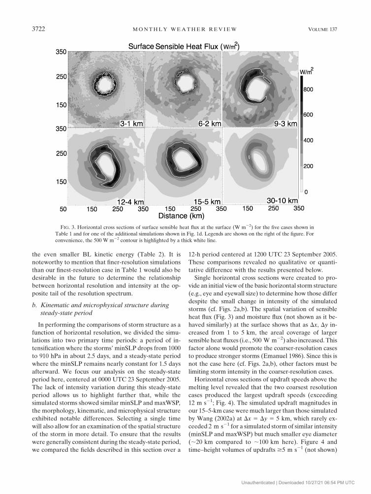
the inner mesh. Figure 3 shows that, for 10-km resolu-

tion, the peak surface sensible heat fluxes (and moisture

flux, not shown) were much weaker than for 5 km by as

much as a factor of 3, consistent with weaker BL kinetic

energy (Table 2). The latter became even smaller as Dx,

Dy increased above 10 km (not shown) as expected from

TABLE 2. The first two columns show the inflow in and vertical mass fluxes (kg m s21) out of a cylinder of radius of 60 km and height of

1.1 km MSL from the storm’s center (defined as the minimum surface pressure). The third column on the right shows the BL integrated

kinetic energy within a cylinder of height 1.1-km MSL and a radius of 120 km from the storm’s center. Inflow and outflow matches within

10% because those were computed from interpolated axisymmetric fields and also because radial inflow used height, not pressure (mass)

coordinates.

Cases Inflow mass flux (3109 kg m s21) Vertical mass flux (3109 kg m s21) BL kinetic energy (3108 m2 s22)

90–30 km Storm center ill defined

60–20 km 22.27 2.94 2.731

45–15 km 22.12 3.5 3.993

30–10 km 26.31 8.19 7.642

15–5 km 29.153 10.15 10.938

12–4 km 29.18 10.55 11.900

9–3 km 27.324 7.871 8.938

6–2 km 24.683 5.146 8.141

3–1 km 25.749 6.253 6.888



the even smaller BL kinetic energy (Table 2). It is

noteworthy to mention that finer-resolution simulations

than our finest-resolution case in Table 1 would also be

desirable in the future to determine the relationship

between horizontal resolution and intensity at the op-

posite tail of the resolution spectrum.

b. Kinematic and microphysical structure duringsteady-state period

In performing the comparisons of storm structure as a

function of horizontal resolution, we divided the simu-

lations into two primary time periods: a period of in-

tensification where the storms’ minSLP drops from 1000

to 910 hPa in about 2.5 days, and a steady-state period

where the minSLP remains nearly constant for 1.5 days

afterward. We focus our analysis on the steady-state

period here, centered at 0000 UTC 23 September 2005.

The lack of intensity variation during this steady-state

period allows us to highlight further that, while the

simulated storms showed similar minSLP and maxWSP,

the morphology, kinematic, and microphysical structure

exhibited notable differences. Selecting a single time

will also allow for an examination of the spatial structure

of the storm in more detail. To ensure that the results

were generally consistent during the steady-state period,

we compared the fields described in this section over a

12-h period centered at 1200 UTC 23 September 2005.

These comparisons revealed no qualitative or quanti-

tative difference with the results presented below.

Single horizontal cross sections were created to pro-

vide an initial view of the basic horizontal storm structure

(e.g., eye and eyewall size) to determine how those differ

despite the small change in intensity of the simulated

storms (cf. Figs. 2a,b). The spatial variation of sensible

heat flux (Fig. 3) and moisture flux (not shown as it be-

haved similarly) at the surface shows that as Dx, Dy in-

creased from 1 to 5 km, the areal coverage of larger

sensible heat fluxes (i.e., 500 W m22) also increased. This

factor alone would promote the coarser-resolution cases

to produce stronger storms (Emanuel 1986). Since this is

not the case here (cf. Figs. 2a,b), other factors must be

limiting storm intensity in the coarser-resolution cases.

Horizontal cross sections of updraft speeds above the

melting level revealed that the two coarsest resolution

cases produced the largest updraft speeds (exceeding

12 m s21; Fig. 4). The simulated updraft magnitudes in

our 15–5-km case were much larger than those simulated

by Wang (2002a) at Dx 5 Dy 5 5 km, which rarely ex-

ceeded 2 m s21 for a simulated storm of similar intensity

(minSLP and maxWSP) but much smaller eye diameter

(;20 km compared to ;100 km here). Figure 4 and

time–height volumes of updrafts $5 m s21 (not shown)

FIG. 3. Horizontal cross sections of surface sensible heat flux at the surface (W m22) for the five cases shown in

Table 1 and for one of the additional simulations shown in Fig. 1d. Legends are shown on the right of the figure. For

convenience, the 500 W m22 contour is highlighted by a thick white line.



FIG. 4. Horizontal (and vertical) cross sections of radar reflectivity at z 5 1.12 km (dBZ) and vertical wind (m s21)

at z 5 8 km at 1200 UTC 23 Sep 2005 for the five cases tested herein. The order of the cases is with the finer-resolution

case shown at the top line and the coarsest simulation case shown at the bottom line. The blue contours in the middle

column plots show vertical wind speed contours less than or equal to 22 m s21 at z 5 2 km and the thick white

contours in the third column plots show wind speed values of 90 m s21. The spatial location of the vertical cross

sections of the third column are shown by a thick black horizontal line on the horizontal cross sections in the first

column. The remaining legends for color and shadings are shown on the right-hand side of the figure.



indicate that the coarser runs had a larger area covered

by those moderate updrafts. The finest-resolution case

revealed a more complex updraft structure: the eyewall

in the finest-resolution cases is composed of numerous

smaller updraft entities of about 2–6 m s21 with isolated

peaks exceeding 10 m s21. Those simulated updraft

magnitudes are in good agreement with Braun’s (2002)

1.3-km MM5 simulation of Hurricane Bob (1991) for a

simulated TC of similar intensity (in terms of minSLP

and maxWSP). Additional horizontal and vertical cross

sections made over a 12-h period centered on 1200 UTC

23 September 2005 (not shown) revealed that in all five

cases the maximum updraft speeds rarely exceeded

15 m s21 in the eyewall, which is an encouraging result

consistent with observations (Jorgensen et al. 1985;

Black et al. 1996). Note the presence of relatively large-

amplitude eyewall asymmetries of radar reflectivity in the

form of wavenumbers 4 and 2 in the 15–5- and 12–4-km

case, respectively (Fig. 4), which have been shown to

act as a brake to storm intensity (Peng et al. 1999; Wu

and Braun 2004; Yang et al. 2007). It is possible

therefore that the gain in intensity by a higher surface

heat flux (and therefore BL kinetic energy; Table 2) at

coarser resolution shown in Fig. 3 is compensated by an

energy loss via large amplitude eyewall asymmetries.

The temporal evolution and persistence of these eye-

wall asymmetries will be analyzed in section 3c.

For the two coarser cases (15–5 and 12–4 km), the

eyewalls were wider (Fig. 4). This is a well-known result

and has already been documented, for instance, by Yau

et al. (2004) in their MM5 simulation of Hurricane

Andrew (1992) as Dx, Dy increased from 2 to 6 km. This

result was also found by Davis et al. (2008) as Dx, Dy was

decreased from 12 to 4 and 1.3 km. Finally, Chen et al.

(2007) found the same result in a MM5 simulation of

Hurricane Floyd (1999) as Dx, Dy was decreased from

15 to 5 and 1.3 km. The larger eyewalls in the two coarser-

resolution cases also produced wider horizontal wind

speed contours exceeding 70 m s21, which as we shall

discuss later promote stronger storm surge.

Analyses based on single cross sections are, however,

limited because of temporal and spatial variations of the

simulated TC’s kinematic and microphysics fields. To

provide a more general description of the microphysical

and kinematic attributes of the storm at that time, radius–

height plots of axisymmetric mean quantities during the

steady-state period were generated. It is relevant to de-

termine to what extent the simulated vertical structure of

averaged fields varies and in turn, how these could fur-

ther isolate factors favoring/limiting storm intensity in

each case. Note that because of the aforementioned

larger eyewall asymmetries at coarser resolution, the

averages values will be smaller than at finer resolution.

With the exception of the coarsest case (15–5 km), the

maximum azimuthal mean of tangential winds (Vtu) at

1.12 km exceeded 80 m s21 (Fig. 5). Additionally, the

surface wind fields for the two coarser-resolution runs

extended farther in radius than the three other cases. As a

result, the integrated BL kinetic energy (as defined by

Powell and Reinhold 2007) of the simulated storm in-

creased as horizontal resolution decreased (Table 2). It is

also worth noting that the eyewall outward slope [defined

here as the angle from the vertical of the axis of the radius

of maximum wind (RMW) or peak Vtu], which here in-

creases as horizontal grid spacing increases, is closely re-

lated to the size of the RMW (Stern and Nolan 2009); that

is, as the RMW decreases, the slope of the eyewall de-

creases (i.e., less vertical tilt; Fig. 5). Typical eyewall slopes

of radar reflectivity in nonsheared environments observed

by radar (Marks 1985) are about 408–458 from the vertical

axis. This is much smaller than the values obtained here

for the two coarser-resolution cases, which were about 758

(Fig. 5). However, the finer-resolution cases revealed ra-

dar reflectivity slope of about 508–608, in closer agreement

with observations (Fig. 6). It is important to note that

similar to observations (Marks and Houze 1987), the slope

of the RMW does not coincide with the slope of azimuthal

mean of reflectivity (Figs. 5 and 6). All five simulations

showed that this result also held for updraft speed and

vertical vorticity, which all appeared to be more upright

(i.e., smaller slope) than the RMW (Figs. 5 and 6). For

updrafts, slopes ranged between 508 and 658 for the three

finer-resolution runs compared to about 758 for the two

coarser-resolution cases while simulated RMW slopes

ranged from ;758 for the 3–1-km case to ;808 in the 15–5-

km case. Yang et al. (2007) showed that storms with larger

eyewall tilt (or slope) were more intense because this tilt

allowed more low-ue downdraft air to reach the subcloud

inflow layer which in turn increased the air–sea entropy

difference there and therefore, the energy input from the

sea. They suggested that storms exhibiting less vertical tilt

(smaller eyewall slope), were less intense because of en-

hanced inward potential vorticity (PV) mixing from the

eye to the eyewall. Our results show, however, that de-

spite larger eyewall slopes, the coarser-resolution cases

still do exhibit relatively similar intensity to those at

finer resolution.

The radius–height mean diagrams in Figs. 5 and 6

show that the horizontal gradients of Vtu, vertical vor-

ticity (zu), and vertical wind (Wu), increase as Dx, Dy

decreases at all levels. Moreover, closer investigation of

the reflectivity field shown in Fig. 4 revealed the exis-

tence of small-scale convective features of about 1–2-km

depth near the surface (only observed for the 3–1- and

6–2-km case) on the inner boundary of the eyewall that

were sometimes associated with well-defined isolated



maxima in wind speed, sometimes reaching 100 m s21 in

the simulation (not shown), consistent with previous

modeling work (Yau et al. 2004) and in situ observations

(Aberson et al. 2006; Marks et al. 2008).

The updrafts in all five cases exhibit a bimodal dis-

tribution with two well-defined maxima: one below the

freezing level (4–5 km) and another one near or above

8 km (Fig. 5). This result is consistent with previous ob-

servational and modeling studies made in mature hurri-

canes (Black et al. 1996) and tropical maritime squall

lines (Samsury and Zipser 1995; May and Rajopadhyaya

1996; Fierro et al. 2008, 2009). The 6-km simulation of

FIG. 5. Height–radius plots of mean azimuthal tangential, radial, and vertical wind speed (m s21) for the five cases

at 1200 UTC 23 Sep 2005. The dotted lines in the third column for vertical wind speed depict the 0 m s21 contour. The

legends for shadings are shown on the right-hand side of the figure.



Liu et al. (1999) also showed evidence of this bimodal

distribution (their Fig. 15c) but the latter was never

discussed. Previous studies suggested that the lower

maximum is mainly attributed to dynamical forcing

(frictional convergence for hurricanes and gust front

upward directed hydrostatic pressure gradient force

for squall lines), while the upper-level maximum could

be a consequence of water unloading and buoyancy

FIG. 6. As in Fig. 5, but for vertical vorticity (31023 s21) and radar reflectivity (dBZ). Note

that for vertical vorticity the radial axis extends to near 160 km compared with 120 km for

radar reflectivity.



(Samsury and Zipser 1995; May and Rajopadhyaya

1996; Trier et al. 1996; Zipser 2003; Fierro et al. 2008,

2009). Black et al. (1996) found in hurricane eyewalls a

relative minimum in updraft speed near 6 km, which

agrees remarkably well with the results obtained herein

for Wu, particularly in the two finer-resolution cases

(Fig. 5). The double maximum in vertical velocity with

radius that is present in the 15–5-km simulation exists

because the storm-centered circles along which the

azimuthal mean is computed covers a wavenumber

4 eyewall asymmetry (Fig. 4). This double maximum

in vertical wind is however not present in the 12–4-km

case because the amplitude of the wavenumber 2 eye-

wall asymmetry in this simulation is too large (i.e.,

large eccentricity) for those circles to cover it entirely

(Fig. 4).

FIG. 7. As in Fig. 5, but for graupel, rain, and snow mixing ratio (g kg21). Note that the radial axis for snow mixing

ratio extends to 160 km instead of 120 km for graupel and rain mixing ratio.



The depth of the inflow layer (defined as the layer

containing negative azimuthally averaged radial wind)

decreased as resolution increased (Fig. 5). In fact, under

the eyewall, this depth doubled from about 1 km in

the 3–1-km case to about 2 km in the 15–5-km case.

Furthermore, the coarser-resolution cases produced

larger azimuthally averaged radial wind speed (by

about 5 m s21) in this inflow layer near the surface

(Fig. 5). Computations of the vertical mass flux and

inflow mass flux in Table 2 for all five cases showed that

at coarser resolution, the simulated storms produced

much larger low-level inward mass flux, which by virtue

FIG. 8. CFADs of vertical wind (W; m s21), radar reflectivity (dBZ), and rain mixing ratio (Qr; g kg21) in bins of

1 m s21, 0.5 g kg21, and 0.5 g kg21, respectively, for all five cases at 1200 UTC 23 Sep 2005. Legends for shadings are

shown on the right side of the figure.



of mass conservation must be consistent with larger

vertical (i.e., updraft) mass flux in the eyewall. This

shows that at coarser resolution, the secondary circu-

lation is stronger, which is consistent with larger sensi-

ble heat/moisture flux and favorable for storm intensity.

Therefore, it appears that at coarser resolution, the

larger areal coverage of strong radial surface fluxes

(consistent with a deeper and stronger secondary cir-

culation) is able to counteract the detrimental effects of

smaller radial gradients and internally generated eyewall

asymmetries, resulting in storms of relatively similar

intensities.

FIG. 9. As in Fig. 8, but for graupel mixing ratio (Qg), snow mixing ratio (Qs; g kg21), and number ice concentration

(Qni; 106 kg21) in bins of 0.5 g kg21, 0.5 g kg21, and 0.5 3 106 kg21, respectively.



Overall, the simulated microphysical structures are

qualitatively consistent with past modeling studies at

similar horizontal resolution (Liu et al. 1997; Wang

2002a; Fierro et al. 2007). As expected from the profiles

of axisymmetirc kinematic variables, the three finer-

resolution cases again exhibited larger values of axi-

symmetric rain, graupel, and snow mixing ratio (e.g.,

Qru, Qgu, and Qsu; Fig. 7) and hence axisymmetric radar

reflectivity (dBZu; Fig. 6). Most importantly, the latter

variables exhibited sharper radial gradients at the inner

edge of the eyewall as horizontal resolution increased.

The reflectivity in the 3–1-km case quickly decreases

radially outward to values below 10 dBZ. On the other

hand, the 6–2- and 9–3-km cases showed evidence of

well-defined secondary azimuthally averaged reflectivity

maximum at radii of 60 and 80 km, respectively. This

secondary reflectivity maximum (also see in Fig. 4) is

coincident in space with weak maxima in Wu, Vtu, and

zu (Figs. 5 and 6). Those characteristics are similar to

the ones associated with secondary concentric eyewalls

(Terwey and Montgomery 2008) and a moat region

(referred to as filamentation zone by Rozoff et al. 2006)

followed by a secondary wind maximum (e.g., Houze

et al. 2007), which were shown to be associated with a

temporary weakening of the storm (Willoughby et al.

1982) and that was actually observed for Hurricane

Rita about a day earlier than shown in our simulations

(Knabb et al. 2005).

In addition to looking at mean values or cross sections

at a single level or location, it is also worthwhile to

examine the properties of the entire distribution of a

variable. This will allow a diagnosis of the impact of

resolution on different portions of a distribution (e.g., to

compare the impact of resolution on the percentage

of updrafts that are strong versus weak). Figures 8–9

show contoured-frequency by altitude diagrams (CFADs:

Fig. 5 in LeMone and Zipser 1980) for select variables.

For the computation of the frequencies, the data was

extracted within a box surrounding the eyewall relative

to a storm center that was defined by the location of the

minimum surface pressure. Since the two coarser runs

had larger eyewalls, the box was allowed to cover a

slightly larger area for those two cases. The distribution

of vertical velocities varied significantly between the

cases at this time. For example, as Dx and Dy increased,

the frequency contour for the strongest (top 0.1%) up-

drafts tends to shift toward higher altitudes (Fig. 8),

while the 0.1% contour of downdrafts reached larger

values in the three finer-resolution cases between 0 and

4 km (particularly for the 3–1-km case with values near

25 m s21). Generally speaking, the updraft distribution

in the eyewall for all five cases agree well with the

composite observations of Black et al. (1996), who found

that the vast majority of vertical motions were weak

(jwj , 2 m s21), although the model seems to produce

generally fewer strong updrafts than what have been

found in Black et al. (1996). Those results are simi-

lar to those of R07 but seem to contradict those of

McFarquhar et al. (2006) who found in their 2-km MM5

simulation more strong updrafts than observed above

9 km. In nature, about 1%–2% of the drafts exceed

5 m s21 (Black et al. 1996), which is in good agreement

with our results (lightest gray shaded contour in Fig. 8) and

those of R07. In all five cases, the distribution of updraft

speeds does not broaden with height as in the observa-

tions, indicating that the strongest updraft cores weaken

with height. This result is similar to previous modeling

results such as R07. The two coarser-resolution cases have

their small frequency contours (top 0.5%) extend-

ing toward larger updraft values (.10 m s21), which is

consistent with stronger secondary circulations (Table 2).

At even coarser resolution (Dx and Dy $ 10 km) the top

0.5% contour dropped below 5 m s21, which is consis-

tent with overall weaker axisymmetric vertical velocities

(not shown).

In contrast with observations in mature hurricanes,

none of the five cases presented herein exhibited a sharp

decrease of reflectivity above the melting level (Fig. 8),

similar to the results of R07. In all cases, we noted an

increase of larger frequencies greater than 2% of 20–25-

and 25–30-dBZ reflectivity bins above 8 km, associated

with an overall small amount of graupel and water drops

and the predominance of snow particles at those levels

(Fig. 9). In nature, both Atlantic hurricanes and tropical

convective clouds exhibit a sharp decrease of radar re-

flectivity (and therefore frequencies of larger reflectivity

bins) above the melting level (R07), with maximum

values in the vast majority of the cases seldom exceeding

50 dBZ (e.g., Marks et al. 2008). The rapid decline of

reflectivity values above the freezing level is mainly at-

tributed to warm rain processes, which leaves very little

supercooled water available in the mixed-phase region

(between 08C and 2208C) for the formation/growth of

graupel and hail (e.g., Black and Hallett 1986). In line

with R07, McFarquhar et al. (2006) and Davis et al.

(2008) we observed a high bias of radar reflectivity par-

ticularly for values larger than 40 dBZ near the surface.

In contrast to the three finer-resolution cases, the

15–5- and 12–4-km cases produced a deeper distribution

of graupel with altitude. This indicates that the stronger

secondary circulation in the coarser runs carried graupel

over a deeper layer, supporting larger volumes of mixed-

phase particles (and therefore latent heating) aloft that

are indicative of strong updrafts (Wiens et al. 2005)

generally exceeding 10 m s21 (McFarquhar et al. 2006).

The 6-km simulation of Liu et al. (1999) also consistently



produced graupel (0.5 g kg21) at rather high altitudes

near 250 hPa. Although the frequency distribution of

snow (and rain) did not exhibit marked trends or dif-

ferences, there is some indication that the wider eye-

walls in the two coarser-resolution cases did produce

more snow: the 0.1% contour for snow reached higher

mixing ratio values (near 8.5 g kg21) for the coarse runs

than for the fine runs (7.5 g kg21; Fig. 9). All cases

showed a well-defined maximum in the frequency of

snow mixing ratio between 0.5 and 1.5 g kg21 between

4 and 8 km (Fig. 9), which is consistent with largest

frequencies of 0.5–1 g kg21 graupel mixing ratio as

more snow particles are available for graupel growth by

rime accretion (Fig. 9). Note that in all five cases a very

small volume (only about 2% of the sampled grids)

had a graupel mixing ratio of about 1 g kg21, consistent

with in situ observations (McFarquhar and Black, 2004).

Near the homogeneous nucleation level (at about 2408C

near z 5 15 km) the three finer-resolution runs pro-

duced higher frequencies of large values of number ice

FIG. 10. Hovmoller diagrams of azimuthally averaged vertical vorticity (31023 s21), tangential wind (Vt; m s21), and

radar reflectivity (dBZ) at z 5 1.12 km. Legends for shadings are shown on the right side of the figure.



concentration (Qni; 2 3 106 kg21; Fig. 9), while the two

coarser cases had larger frequencies toward smaller Qni

values (0.5 3 106 kg21). Aircraft penetrations in Hurricane

Humberto (2001) at temperatures near 2408C revealed

maximum ice particle size concentrations ranging be-

tween 200 and 300 L21 (Heymsfield et al. 2006), which is

equivalent to about 1.2 and 1.8 3 106 kg21 when ac-

counting for density variations with altitude. Hence, the

modeled values at finer resolution tend to agree better

with observations.

c. Kinematic and microphysical evolution duringthe intensification phase

After focusing on the spatial structure of the simu-

lated storm at a single time, this section will be devoted

to its temporal evolution, which will help to further

FIG. 11. As in Fig. 10, but for azimuthally averaged vertical wind speed (W; m s21), graupel mixing ratio (Qg;

g kg21) at z 5 5.91 km, and rain mixing ratio (Qr; g kg21) at z 5 1.12 km. The dotted line in the W plots marks the

zero contour.



identify factors promoting/limiting storm intensity. To

provide a comprehensive view of the kinematic and

microphysical evolution, we generated time–radius (i.e.,

Hovmoller) plots of axisymmetric means, where the

storm’s center is defined at each altitude as the minimum

in the smoothed geopotential field. Allowing the storm

center to vary with height will mask some of the asym-

metries in the vertical and in the horizontal that many

observational and modeling studies have suggested are

essential to hurricane intensity and motion (e.g., Marks

et al. 1992; Liu et al. 1999; Shapiro and Franklin 1999;

Reasor et al. 2000; Rogers et al. 2003; Nolan et al. 2007).

The 3–1-km simulation develops a well-defined (.5 3

1023 s21) ring of positive azimuthal-mean vertical vor-

ticity (zu) at z 5 1.12 km 36 h into the simulation (here-

after the subscript u refers to azimuthally averaged

variables; Fig. 10). While the magnitude of this vorticity is

larger than the other four runs, its development occurs

later than the other runs. The RMW varies from ;40 to

;60 km in the 3–1- and 15–5-km cases, respectively, with

even larger values for Dx, Dy $ 10 km (e.g., ;90 km for

the 60–20-km run, not shown). Aircraft data found that

the eye diameter was about 35 km at Rita’s peak intensity

(Knabb et al. 2005), so the observed RMW was about

10 km smaller than the smallest RMW in the 3–1 km run.

Previous modeling studies have often produced generally

larger simulated RMW’s compared to the observations

while still producing pressure minima and wind speed

maxima similar to observations (e.g., R07; Fierro et al.

2007). Davis et al. (2008) suggested that storm size was

likely influenced by model resolution (and drag formu-

lation) and increased as Dx, Dy increased, as suggested by

Liu et al. (1999) and shown by Yau et al. (2004). Kimball

and Mulekar (2004) found that the median RMW de-

creases with storm intensity, from about 60 km for cate-

gory 1 storms to 40 km for category 5 storms. However, a

recent analysis of in situ observations of hurricane wind

fields by Stern and Nolan (2009) has shown that there is a

strong relationship between the size of the RMW and the

slope of the eyewall, where larger (smaller) RMWs are

associated with larger (smaller) slopes; they also found

that neither storm size nor eyewall slope is correlated

with intensity. Stern and Nolan (2009) also found that the

RMW–slope relationship, as well as its independence

from intensity, could be shown explicitly from the maxi-

mum potential intensity theory of Emanuel (1986). A

similar relationship was seen for these runs (Figs. 5 and

10). This suggests that the WRF-ARW model captures

this essential aspect of storm dynamics as resolution

varied between 1 and 5 km.

All cases behave qualitatively the same; the increase

in Vtu and zu (at 1.12 km) during intensification is

coincident with an increase in the azimuthal mean

of graupel mixing ratio (Qgu), rain mixing ratio (Qru),

radar reflectivity (dBZu), and vertical velocity (Wu;

Figs. 10 and 11) suggesting that storm becomes better

organized and circular. For all these variables, the three

finer-resolution runs exhibited overall better-defined

radial profiles (cf. Figs. 5–8) in the eyewall throughout

the simulation, consistent with radial gradients being

better resolved, which would promote storm intensity.

To see how the mean properties of certain fields

evolve in height and time, we computed time–height

plots of updraft and downdraft mass fluxes above or

below a predefined threshold within a predefined box,

which dimensions were selected such that the box covers

the eyewall (and eye). Also, because eyewall convection

sloped outward, we used vertical cross sections to de-

termine the dimensions of this predefined box to ensure

that the latter also contained the upper-level updrafts

and a good portion of the outer eyewall stratiform re-

gion. For microphysical quantities, we used a different

approach and computed time–height volume plots in the

following manner: for each grid point having any given

variable equaling or exceeding a preset threshold value

we counted the volume occupied by that grid element

using an average value of dz (i.e., 472 m) based on the

model top and number of grid points in the vertical (as in

Fierro et al. 2006). The advantage of using hydrometeor

volumes over hydrometeor mass fluxes is that the latter

involves the product of mixing ratio and vertical veloc-

ity, while volumes just make use of mixing ratio. In our

context, this makes comparisons among cases easier as

hydrometeor volumes are more directly related to hy-

drometeor content or mass. Information about the ver-

tical distribution of total microphysical quantities will

provide key insight on the temporal evolution of the

vertical distribution of latent heat (e.g., Gray 1995) and

therefore PV (e.g., Yang et al. 2007).

As expected from overall larger eyewalls and wider

updrafts, the two coarser runs exhibit much larger total

updraft mass flux, updraft mass flux for updrafts $5 m s21

(W5), and total downdraft mass flux than the three re-

maining cases at almost all levels (particularly above

7 km; Fig. 12a). Consequently, the 0.5 g kg21 rain mixing

ratio (Qrvol), 0.5 g kg21 graupel mixing ratio (Qgvol),

and 30-dBZ echo (dBZvol) volume were larger in the two

coarser-resolution runs (Fig. 13) and are consistent with

the CFADs for graupel and rain showing increased

frequencies toward larger values (Figs. 7 and 8). These

further support the notion that at coarser resolution the

simulated storms exhibit stronger secondary circula-

tions, which carry a larger volume of condensate aloft

and therefore produce more latent heating. The simu-

lated eyewall total downdrafts and updraft mass flux

values are comparable to those observed by Black et al.



FIG. 12. (a) Time–height plots from left to right of total updraft mass flux, total downdraft mass flux, and updraft

mass flux for updrafts $5 m s21 (kg s21) for the five cases within a predefined box containing the eye and eyewall.

Legends for shadings are shown on the right side of the figure. (b) From left to right the fraction of the mass flux for

updraft $1 m s21 (W1) relative to the total updraft mass flux (W1), the mass flux for updraft $5 m s21 (W5) relative

to W1 and the mass flux for downdrafts #22 m s21 (W22) relative to the total downdraft mass flux (W2).



(1996, their Fig. 16), after accounting for the fact that the

Black et al. (1996) vertical mass fluxes were scaled by a

factor of 2p (their formulas 3 and 4) due to the use of

cylindrical coordinates. As Dx, Dy $ 10 km, the total

updraft fluxes and hydrometeor volumes progressively

became smaller, consistent with a weaker secondary

circulation (Table 2) and overall weaker vertical veloc-

ities (not shown).

The simulations revealed that updrafts $5 m s21 did

show a remarkably similar contribution to the total up-

draft mass flux in all five cases: below 3 km, their con-

tribution was less than 10% while between 4 and 8 km,

they contributed to between 30% and 50% of the total

updraft mass flux (Fig. 12b), which is in good agreement

with Jorgensen et al.’s (1985) statistics of in situ obser-

vations within mature hurricanes (their Fig. 7). Perhaps

FIG. 12. (Continued)



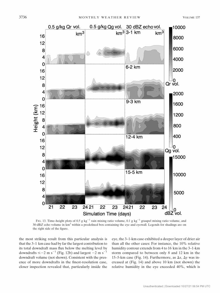
the most striking result from this particular analysis is

that the 3–1 km case had by far the largest contribution to

its total downdraft mass flux below the melting level by

downdrafts #22 m s21 (Fig. 12b) and largest 22 m s21

downdraft volume (not shown). Consistent with the pres-

ence of more downdrafts in the finest-resolution case,

closer inspection revealed that, particularly inside the

eye, the 3–1-km case exhibited a deeper layer of drier air

than all the other cases: For instance, the 10% relative

humidity contour extends from 4 to 16 km in the 3–1-km

storm compared to between only 8 and 12 km in the

15–5-km case (Fig. 14). Furthermore, as Dx, Dy was in-

creased at (Fig. 14) and above 10 km (not shown) the

relative humidity in the eye exceeded 40%, which is

FIG. 13. Time–height plots of 0.5 g kg21 rain mixing ratio volume, 0.1 g kg21 graupel mixing ratio volume, and

30-dBZ echo volume in km3 within a predefined box containing the eye and eyewall. Legends for shadings are on

the right side of the figure.



consistent with weaker secondary circulations (Table 2)

and weaker storms (Fig. 2). This drier air at finer re-

solution is also reflected in the equivalent potential

temperature (ue) profile. The simulated minimum in the

3–1-km run (near 358 K) was about 108 lower than the

15–5-km case (about 369 K, not shown). A subsequent

study using trajectory analysis with relatively finer tem-

poral resolution than used herein (1 h or less is desired)

will be performed in the near future to address if the

downdrafts in the eye are the cause or the consequence

of the presence of this deeper layer of drier air and in

turn determine to what extent this dry air mixes with the

eyewall convection and influences downdraft potential

and storm intensity.

In the previous section, we showed that during the

steady-state period, the coarser-resolution cases exhib-

ited larger-amplitude eyewall asymmetries (cf. Fig. 4),

which has been shown to act as a potential brake on

storm potential intensity (Peng et al. 1999; Wu and

Braun 2004; Yang et al. 2007). Therefore it is relevant to

determine their temporal evolution and persistence. To

quantify the amplitude of the eyewall asymmetries and

their evolution, we carried out a fast Fourier transform

(FFT) on the radar reflectivity at z 5 1.5 km averaged

along circles at and inside about 10 km of the RMW

(Fig. 15), similar to what was done in radar observations

of Hurricane Elena (1995; Corbosiero et al. 2006). Re-

cently, Murillo et al. (2009, manuscript submitted to

Mon. Wea. Rev.) compared single Doppler retrieved

wavenumber 0 and 1 reflectivity and wind structures for

Hurricane Danny (1997). They pointed out that while

the wavenumber 0 structures were similar the phase and

amplitude on the wavenumber 1 asymmetries were not.

In the light of those results, an additional FFT analysis

was carried out on the simulated horizontal wind speeds

(z 5 1 km) and revealed that the results were almost

identical to those using radar reflectivity (not shown).

We will focus our analysis after 0000 UTC 22 September

2005, which is the time when the simulated storms ex-

hibited a well-defined eyewall in all five cases. We no-

ticed that, particularly in the three finer-resolution cases,

the darkest shaded contours (indicating high power ratio

relative to the azimuthal mean) are essentially confined

in the axisymmetric flow and wavenumber 1 asymmetry,

which shows that most of the variance (or power) in the

reflectivity field is contained in the axisymmetric mean

and wavenumber 1 asymmetries. Those results are sim-

ilar with what previous studies have found for the hori-

zontal flow within observed hurricanes (Lee et al. 1994,

2000; Roux and Marks 1996; Reasor et al. 2000; Lonfat

et al. 2004; Corbosiero et al. 2006). Most importantly,

relative to the highest power, the two coarser cases have

a higher proportion of large power values contained in

wavenumber 1, 2, and 3 asymmetries, indicative of larger

amplitudes of these asymmetries, a result that is consistent

with Gentry and Lackmann (2010). Those larger-

amplitude eyewall asymmetries explain why axisymmet-

ric means are generally smaller in the two coarser cases

FIG. 14. As in Fig. 5, but for relative humidity (%).



(Figs. 10 and 11). Additional power spectra plots that

extend to higher wavenumbers (i.e., greater than 6) re-

vealed that the 3–1-km case exhibited larger power values

for these high-wavenumber asymmetries than the coarse

runs, though the magnitude of the power is much less

than the lower-wavenumber asymmetries (not shown).

At even coarser resolution, (Dx, Dy $ 10 km), the ma-

jority of the eyewall asymmetries power was contained in

wavenumber 1 (not shown). This tendency toward lower

wavenumber at coarser resolution is mainly due to the

poor azimuthal resolution in the eye, which can ade-

quately resolve only the lowest wavenumbers. Schubert

et al. (1999) also showed that lower wavenumbers

are favored for wider eyewalls. Modeling (Kossin and

Schubert 2001; Wang 2002b) and observational (Kossin

and Schubert 2004; Montgomery et al. 2006) studies have

suggested that those eyewall asymmetries were associ-

ated with vortex Rossby waves or coherent vortices along

the inner edge of the eyewall convection.

4. Discussion and conclusions

In summary, we found that changing the horizontal

grid spacing from 5 to 1 km did not result in significant

changes in maximum intensity (defined as the 10-m

maximum wind speed and minimum sea level pressure),

while in contrast, noteworthy differences in the simulated

storms’ kinematics and microphysics were found. Those

structural differences were consistent through both the

intensification and steady-state periods. Larger grid

spacing resulted in larger eyewalls producing larger mass

flux and volume of updrafts and, consequently, larger

volumes of condensate, and ice-phased particles. In con-

trast, the opposite was true for downdrafts #22 m s21,

which were found to produce by far the largest contribu-

tion to the total downdraft mass flux at finer grid spacing.

Although the coarser-resolution cases consistently pro-

duced larger mass flux of updrafts $5 m s21, it was found

that their contribution to the total mass flux varied little

among the five cases. Hence, in all cases the bulk of the

mass is being transported by the smaller drafts (and

secondary circulation). The RMW and eyewall slope

(defined as the axis of maximum Vtu) were also shown to

increase as horizontal grid spacing increased, which is

consistent with observations showing that eyewall slopes

increase as RMW increases (Stern and Nolan 2009).

Vertical profiles of microphysical and kinematical

variables at finer grid spacings were generally radially

thinner as smaller updrafts were better resolved. The

smaller azimuthal means of these variables at coarse

resolution were attributed to larger-amplitude lower-

wavenumber eyewall asymmetries, while at finer grid

spacing, the eyewall asymmetries were of lower ampli-

tude and higher wavenumber (greater than 6).

The simulations also revealed structural similarities

among the five cases, which held during both the

intensification and steady-state periods. For instance, all

storms exhibited a bimodal updraft distribution and

were able to reproduce the basic aspects of the primary

and secondary circulation. Also, all cases produced rel-

atively similar vertical distribution of rain, snow, and

radar reflectivity in their eyewall.

One way to test the robustness of the differences

shown here is to compare the structures produced from

models of different resolution on a uniform grid. This

FIG. 15. Fourier spectral decomposition of eyewall wavenumber

asymmetries of radar reflectivity at z 5 1.5 km averaged along

several circles centered at the minimum geopotential height. The

ring where the average was carried out is shown at the bottom. The

dark filled contour show the log-10 of Fourier coefficient power

divided by the log-10 power of the azimuthal mean. Legends are

shown on the right side of the figure.



can be done by carrying out a volume average of the

simulated fields of the finer grid onto the coarser grid

(e.g., R07; Dr. J. Reisner 2009, personal communica-

tion). Figure 16 shows selected key fields averaged

from the finest-resolution case (1-km inner mesh)

onto a 5-km mesh (since Dz was identical, we carried

out an areal average in this case), which facilitates a

more direct comparison of the two simulations. When

the volume-averaged profiles (CFAD and radius–

height means) of the 1-km grid are compared with

those of the 15–5-km case, we found that, similar to R07

(their Fig. 13), the averaging did not change the simu-

lated profile significantly but rather smoothed out the

fields and reduced the peak values/contours. There-

fore, we can confidently affirm that the comparisons

made herein remain valid.

An obvious question to ask based on these results is

why the simulated storms showed little difference in in-

tensity evolution between 1- and 5-km grid length despite

noteworthy structural differences as a function of hori-

zontal resolution. Across the (rather narrow) spectrum of

resolutions compared in detail here, there were numerous

factors that either limited or promoted storm intensifi-

cation as resolution varied. For example, factors limiting

storm intensification at coarser resolution were larger

amplitude low-wavenumber eyewall asymmetries and

smaller radial gradients, while the limiting factor at finer

resolution was mainly a smaller areal coverage of larger

surface sensible and moisture fluxes. Conversely, factors

favoring storm intensification at coarser resolution were

the larger areal coverage of stronger surface fluxes

(consistent with larger BL kinetic energy), while at finer

resolution the larger radial gradients and smaller am-

plitude low-wavenumber eyewall asymmetries favored

stronger storm intensity. Given the resultant similarity in

intensity evolution, these factors must have compensated

for each other, causing the simulated storms’ intensities to

be relatively similar for different resolution despite

exhibiting noticeable structural differences.

In contrast, as Dx, Dy in the inner mesh was further

increased from 10 km up to 30 km, the storm intensity

showed a rapid decline: the strength of the secondary

circulation, measured by the inflow mass flux and updraft

mass flux, showed a progressive weakening (Table 2),

which was consistent with smaller hydrometeor mass

aloft (not shown) and weaker updraft speeds. A similar

trend was simulated for the BL kinetic energy (Table 2),

which also indicated progressively weaker near-surface

wind fields. If we consider a typical eye diameter of

40 km, a mesh of 10 km would represent the lower limit

at which the eyewall could be resolved. This limitation,

together with much weaker radial gradients, are the

likely causes for the storm intensity to drop off dra-

matically as Dx, Dy exceeds the 10-km threshold.

From the standpoint of accurately representing the

kinematic and microphysical structures at different

FIG. 16. Radius–height mean diagrams and CFADs for key variables of the 3–1-km case averaged onto a 5-km grid.

Legends for contouring and shadings are the same as the above corresponding figures and are therefore omitted.



horizontal resolutions, the finer-resolution cases, par-

ticularly 3–1 km, exhibited a more realistic storm,

which suggests that horizontal resolution is important

in resolving small-scale structures (Yau et al. 2004;

Chen et al. 2007), some of which could be important in

determining storm intensity (e.g., small-scale meso-

vortices) and rapid intensity changes, which are cur-

rently poorly modeled (Davis et al. 2008). In the future,

further studies at finer horizontal grid spacing (Dx, Dy ,

500 m) are needed to determine if our results hold be-

cause the flow characteristics were shown to change

when Dx, Dy , 250 m (Bryan et al. 2003), with an in-

creasing turbulent regime and increasing importance of

entrainment effects. While these results were obtained in

thunderstorm simulations, they should also be tested in

hurricane environments.

At the range of cloud-resolving grid spacings used

here it appears that axisymmetric differences in these

structures do not translate to significant changes in the

10-m maximum wind speed. Again, similar analysis us-

ing finer grid spacings are required to determine if

horizontal resolution alone (i.e., using similar physical

parameterizations) can significantly improve intensity

forecasts as posited by Houze et al. (2007). The current

study suggests that this might not be the case and that,

rather, more improvements in the representation of the

model physics, particularly the atmospheric boundary

layer (McFarquhar et al. 2006), and storm initialization

using real-time data assimilation (as in Zhang et al.

2009) are needed to improve TC intensity forecasts.

Further tests at higher horizontal resolution and with a

variety of physical parameterizations and initial vortex

structures for several strong storm cases are required to

better address this hypothesis. Recently, using similar

physics and settings within the ARW model, Gentry and

Lackmann (2010) carried out a similar analysis for

Hurricane Ivan (2004) and showed that as Dx, Dy, was

increased from 1 to 6 km, the minSLP could differ by as

much as 20 mb, while the structural differences as a

function of horizontal resolution were comparable

to those found here. Hence, while different physical/

dynamical processes influence modeled intensity and

their respective weight vary as a function of Dx, Dy it

seems that also the latter can change as a function of the

storm case being studied.

Another reason why little difference was seen in the

intensity of the simulated storms at different resolutions

may be because of the way in which storm intensity is

defined. If intensity were to be defined as the integrated

surface (or even boundary layer) wind speed or kinetic

energy, then the two coarser cases clearly produced

‘‘stronger’’ storms (Table 2). The wider and broader

tropical storm force wind field observed in those two

cases would likely result in larger wind swaths and,

therefore, more widespread and stronger storm surges.

This result alone points out the misleading notion of

using one metric to judge the performance of the model,

particularly one not representative of the storm struc-

ture (e.g., 10-m maximum wind speed). Based on obser-

vations of mature hurricanes, the three finer-resolution

cases tended to produce more realistic, ‘‘tighter’’ eye-

walls with occasional rainbands, the latter being ill de-

fined in the two coarser runs (as in Davis et al. 2008).

Consequently the two coarser-resolution cases would

tend to overestimate the simulated wind swath and

storm surge, parameters that are critical when evacua-

tion orders must be issued for coastal communities

prone to storm surge. Moreover, structural details in the

convection are also important when forecasting coastal

and inland flooding. Our simulation showed that for

instance the rainbands started to become better resolved

at Dx, Dy 5 3 km. Therefore, we suggest that in order to

improve forecast of both, storm surge and flooding, a

horizontal grid spacing of 3 km or less should be used in

operational models.

Acknowledgments. We thank The Office of National

Research Council (NRC) from the National Academy

of Sciences for generously sponsoring Alexandre Fierro

for one year and the Oklahoma Supercomputing Center

for Education and Research (OSCER) for providing

computing resources. Partial support was also provided

under the NASA Grant NAG5-10963. We also thank

S. Gopalakrishnan, P. Willis, and the anonymous re-

viewers for providing helpful suggestions on an earlier

version of the manuscript.

REFERENCES

Aberson, S. D., M. T. Montgomery, M. Bell, and M. Black, 2006:

Hurricane Isabel (2003): New insights into the physics of in-

tense storms. Part II: Extreme localized wind. Bull. Amer.

Meteor. Soc., 87, 1349–1354.

Black, M. L., R. W. Burpee, and F. D. Marks, 1996: Vertical motion

characteristics of tropical cyclones determined with airborne

Doppler radial velocities. J. Atmos. Sci., 53, 1887–1909.

Black, R. A., 1990: Radar reflectivity–ice water content relation-

ships for use above the melting layer in hurricanes. J. Appl.

Meteor., 29, 955–961.

——, and J. Hallett, 1986: Observations of the distribution of ice in

hurricanes. J. Atmos. Sci., 43, 802–822.

——, and ——, 1999: Electrification of the hurricane. J. Atmos. Sci.,

56, 2004–2028.

Braun, S. A., 2002: A cloud-resolving simulation of Hurricane Bob

(1991): Storm structure and eyewall buoyancy. Mon. Wea.

Rev., 130, 1573–1592.

——, and W.-K. Tao, 2000: Sensitivity of high-resolution simula-

tions of Hurricane Bob (1991) to planetary boundary layer

parameterizations. Mon. Wea. Rev., 128, 3941–3961.



Bryan, G. H., 2006: The dynamics of the trailing stratiform region of

squall lines. Colloquium, National Severe Storms Laboratory.

——, and R. Rotunno, 2005: Statistical convergence in simulated

moist absolutely unstable layers. Preprints, 11th Conf. on

Mesoscale Processes, Albuquerque, NM, Amer. Meteor. Soc.,

1M.6. [Available online at http://ams.confex.com/ams/

32Rad11Meso/techprogram/paper_96719.htm.]

——, J. C. Wyngaard, and J. M. Fritsch, 2003: Resolution re-

quirements for the simulation of deep moist convection. Mon.

Wea. Rev., 131, 2394–2416.

Chen, S. S., J. F. Price, W. Zhao, M. A. Donelan, and E. J. Walsh,

2007: The CBLAST-Hurricane Program and the next-generation

fully coupled atmosphere–wave–ocean models for hurricane

research and prediction. Bull. Amer. Meteor. Soc., 88, 311–

317.

Corbosiero, K. L., J. Molinari, A. R. Aiyyer, and M. L. Black, 2006:

The structure and evolution of Hurricane Elena (1985). Part II:

Convective asymmetries and evidence for vortex Rossby waves.

Mon. Wea. Rev., 134, 3073–3091.

Davis, C., and Coauthors, 2008: Prediction of landfalling hurri-

canes with the Advanced Hurricane WRF Model. Mon. Wea.

Rev., 136, 1990–2005.

Dougherty, F., and S. Kimball, 2006: The sensitivity of hurricane

simulations to the distribution of vertical levels. Preprints,

27th Conf. on Tropical Meteorology, Monterey, CA, Amer.

Meteor. Soc.

Emanuel, K. A., 1986: An air-sea interaction theory for tropical

cyclone. Part I: Steady state maintenance. J. Atmos. Sci., 43,

585–604.

——, 1988: The maximum intensity of hurricanes. J. Atmos. Sci., 45,

1143–1155.

Fierro, A. O., M. S. Gilmore, E. R. Mansell, L. J. Wicker, and

J. M. Straka, 2006: Electrification and lightning in an idealized

boundary-crossing supercell simulation of 2 June 1995. Mon.

Wea. Rev., 134, 3149–3172.

——, L. M. Leslie, E. R. Mansell, J. M. Straka, D. R. MacGorman,

and C. Ziegler, 2007: A high resolution simulation of the

microphysics and electrification in an idealized hurricane-

like vortex. Meteor. Atmos. Phys., 98, 13–33, doi:10.1007/

s00703-006-0237-0.

——, ——, ——, and ——, 2008: Numerical simulations of

the electrification and microphysics of the weakly electri-

fied 9th February 1993 TOGA COARE squall line, 2008:

Comparisons with observations. Mon. Wea. Rev., 136, 364–

379.

——, J. Simpson, M. A. LeMone, J. M. Straka, and B. F. Smull,

2009: On how hot towers fuel the Hadley cell: Observa-

tional and modeling study of line-organized convection in

the equatorial trough from TOGA COARE. J. Atmos. Sci., 66,

2730–2746.

Gentry, M. S., and G. Lackmann, 2010: Sensitivity of simulated

tropical cyclone structure and intensity to horizontal resolu-

tion. Mon. Wea. Rev., in press.

Goerss, J. S., 2006: Prediction of tropical cyclone track forecast

error for Hurricanes Katrina, Rita, and Wilma. Preprints, 27th

Conf. on Hurricanes and Tropical Meteorology, Monterey,

CA, Amer. Meteor. Soc., 11A.1.

Gray, W. M., 1995: Tropical cyclones. Colorado State University

Rep., World Meteorological Organization, 163 pp.

Heymsfield, A. J., A. Bansemer, S. L. Durden, R. L. Herman, and

T. P. Bui, 2006: Ice microphysics observations in Hurricane

Humberto: Comparison with non-hurricane-generated ice

cloud layers. J. Atmos. Sci., 63, 288–308.

Hong, S. Y., J. Dudhia, and S. H. Chen, 2004: A revised ap-

proach to ice microphysical processes for the bulk parame-

terization of clouds and precipitation. Mon. Wea. Rev., 132,

103–120.

Houze, R. A., S. S. Chen, B. F. Smull, W.-C. Lee, and M. M. Bell,

2007: Hurricane intensity and eyewall replacement. Science,

315, 1235–1239.

Janjic, Z. I., 1994: The step-mountain eta coordinate model:

Further developments of the convection, viscous layer,

and turbulence closure schemes. Mon. Wea. Rev., 122, 927–

945.

Jorgensen, D. P., E. J. Zipser, and M. A. LeMone, 1985: Verti-

cal motions in intense hurricanes. J. Atmos. Sci., 42, 839–

856.

Kain, J. S., and J. M. Fritsch, 1993: Convective parameterization for

mesoscale models: The Kain-Fritsch scheme. The Represen-

tation of Cumulus Convection in Numerical Models, Meteor.

Monogr., No. 24, Amer. Meteor. Soc., 165–170.

Kessler, E., 1969: On the Distribution and Continuity of Water

Substance in Atmospheric Circulations. Meteor. Monogr., No.

32, Amer. Meteor. Soc., 84 pp.

Kimball, S. K., and M. S. Mulekar, 2004: A 15-year climatology of

North Atlantic tropical cyclones. Part I: Size parameters.

J. Climate, 17, 3555–3575.

Knabb, R. D., J. R. Rhome, and D. P. Brown, 2005: Tropical cy-

clone report: Hurricane Rita. Technical Rep., National Hur-

ricane Center, National Oceanographic and Atmospheric

Administration, 33 pp. [Available online at http://www.nhc.

noaa.gov/2005atlan.shtml.]

Kossin, J. P., and M. D. Eastin, 2001: Two distinct regimes in the

kinematic and thermodynamic structure of the hurricane eye

and eyewall. J. Atmos. Sci., 58, 1079–1090.

——, and W. H. Schubert, 2001: Mesovortices, polygonal flow

patterns, and rapid pressure falls in hurricane-like vortices.

J. Atmos. Sci., 58, 2196–2209.

——, and ——, 2004: Mesovortices in Hurricane Isabel. Bull.

Amer. Meteor. Soc., 85, 151–153.

Lee, W.-C., F. D. Marks, and R. E. Carbone, 1994: Velocity Track

Display—A technique to extract real-time tropical cyclone

circulations using a single airborne Doppler radar. J. Atmos.

Oceanic Technol., 11, 337–356.

——, B. J.-D. Jou, P.-L. Chang, and F. D. Marks, 2000:

Tropical cyclone kinematic structure retrieved from single

Doppler radar observations. Part III: Evolution and struc-

ture of Typhoon Alex (1987). Mon. Wea. Rev., 128, 3982–

4001.

LeMone, M. A., and E. J. Zipser, 1980: Cumulonimbus vertical

velocity events in GATE. Part I: Diameter, intensity, and mass

flux. J. Atmos. Sci., 37, 2444–2457.

Lin, Y.-L., R. D. Farley, and H. D. Orville, 1983: Bulk parame-

terization of the snow field in a cloud model. J. Climate Appl.

Meteor., 22, 1065–1092.

Liu, Y., D. L. Zhang, and M. K. Yau, 1997: A multiscale nu-

merical study of Hurricane Andrew (1992). Part I: Explicit

simulation and verification. Mon. Wea. Rev., 125, 3073–

3093.

——, ——, and ——, 1999: A multiscale numerical study of Hurricane

Andrew (1992). Part II: Kinematics and inner-core structures.

Mon. Wea. Rev., 127, 2597–2616.

Lonfat, M., F. D. Marks, and S. Chen, 2004: Precipitation distri-

bution in tropical cyclones using the tropical rainfall measuring

mission (TRMM) microwave imager: A global perspective.

Mon. Wea. Rev., 132, 1645–1660.



Marks, F. D., 1985: Evolution of the structure of precipitation in

Hurricane Allen (1980). Mon. Wea. Rev., 113, 909–930.

——, and R. A. Houze, 1987: Inner core structure of Hurricane

Alicia from airborne Doppler radar observations. J. Atmos.

Sci., 44, 1296–1317.

——, and L. K. Shay, 1998: Landfalling tropical cyclones: Forecast

problems and associated research opportunities. Bull. Amer.

Meteor. Soc., 79, 305–323.

——, R. A. Houze, and J. F. Gamache, 1992: Dual-aircraft inves-

tigation of the inner core of Hurricane Norbert. Part I: Kine-

matic structure. J. Atmos. Sci., 49, 919–942.

——, P. G. Black, M. T. Montgomery, and R. W. Burpee, 2008:

Structure of the eye and eyewall of Hurricane Hugo (1989).

Mon. Wea. Rev., 136, 1237–1259.

May, P. T., and D. K. Rajopadhyaya, 1996: Wind profiler obser-

vations of vertical motion and precipitation microphysics of a

tropical squall line. Mon. Wea. Rev., 124, 621–633.

McFarquhar, G. M., and R. A. Black, 2004: Observations of par-

ticle size and phase in tropical cyclones: Implications for me-

soscale modeling of microphysical processes. J. Atmos. Sci.,

61, 422–439.

——, H. Zhang, G. Heymsfield, R. Hood, J. Dudhia,

J. B. Halverson, and F. Marks, 2006: Factors affecting the

evolution of Hurricane Erin (2001) and the distributions of

hydrometeors: Role of microphysical processes. J. Atmos. Sci.,

63, 127–150.

Mellor, G. L., and T. Yamada, 1982: Development of turbulence

closure model for geophysical fluid problems. Rev. Geophys.

Space Phys., 20, 851–875.

Michalakes, J., J. Dudhia, D. Gill, T. Henderson, J. Klemp,

W. Skamarock, and W. Wang, 2005: The Weather Research

and Forecast Model: Software architecture and performance.

Proceedings of the 11th ECMWF Workshop on High Perfor-

mance Computing in Meteorology, G. Mozdzynski, Ed., World

Scientific, 156–168.

Molinari, J., and M. Dudek, 1992: Parameterization of convective

precipitation in mesoscale numerical models: A critical re-

view. Mon. Wea. Rev., 120, 326–344.

Montgomery, M. T., M. M. Bell, S. D. Aberson, and M. L. Black,

2006: Hurricane Isabel (2003): New insights into the physics

of intense storms. Part I: Mean vortex structure and maxi-

mum intensity estimates. Bull. Amer. Meteor. Soc., 87, 1335–

1347.

Nolan, D. S., Y. Moon, and D. P. Stern, 2007: Tropical cyclone

intensification from asymmetric convection: Energetics and

efficiency. J. Atmos. Sci., 64, 3377–3405.

Peng, M. S., B. F. Jeng, and R. T. Williams, 1999: A numerical study

on tropical cyclone intensification. Part I: Beta effect and

mean flow effect. J. Atmos. Sci., 56, 1404–1423.

Powell, M. D., 1990a: Boundary layer structure and dynamics in

outer hurricane rainbands. Part I: Mesoscale rainfall and ki-

nematic structure. Mon. Wea. Rev., 118, 891–917.

——, 1990b: Boundary layer structure and dynamics in outer hur-

ricane rainbands. Part II: Downdraft modification and mixed

layer recovery. Mon. Wea. Rev., 118, 918–938.

——, and T. A. Reinhold, 2007: Tropical cyclone destructive po-

tential by integrated kinetic energy. Bull. Amer. Meteor. Soc.,

88, 513–526.

Reasor, P. D., M. T. Montgomery, F. D. Marks, and J. F. Gamache,

2000: Low-wavenumber structure and evolution of the hurri-

cane inner core observed by airborne dual-Doppler radar.

Mon. Wea. Rev., 128, 1653–1680.

Rogers, R. F., S. Chen, J. Tenerelli, and H. Willoughby, 2003:

A numerical study of the impact of vertical shear on the dis-

tribution of rainfall in Hurricane Bonnie (1998). Mon. Wea.

Rev., 131, 1577–1599.

——, M. L. Black, S. S. Chen, and R. A. Black, 2007: An evaluation

of microphysics fields from mesoscale model simulations of

tropical cyclones. Part I: Comparisons with observations.

J. Atmos. Sci., 64, 1811–1834.

Roux, F., and F. D. Marks, 1996: Extended Velocity Track Display

(EVTD): An improved processing method for Doppler radar

observations of tropical cyclones. J. Atmos. Oceanic Technol.,

13, 875–899.

Rozoff, C. M., W. H. Schubert, B. D. McNoldy, and J. P. Kossin,

2006: Rapid filamentation zones in intense tropical cyclones.

J. Atmos. Sci., 63, 325–340.

Rutledge, S. A., and P. V. Hobbs, 1983: The mesoscale and mi-

croscale structure and organization of clouds and precipitation

in midlatitude cyclones. VIII: A model for the ‘‘seeder-

feeder’’ process in warm-frontal rainbands. J. Atmos. Sci., 40,

1185–1206.

——, and ——, 1984: The mesoscale and microscale structure and

organization of clouds and precipitation in midlatitude cy-

clones. XII: A diagnostic modeling study of precipitation

development in narrow cold-frontal rainbands. J. Atmos. Sci.,

41, 2949–2972.

Samsury, C. E., and E. J. Zipser, 1995: Secondary wind maxima in

hurricanes: Airflow and relationship to rainbands. Mon. Wea.

Rev., 123, 3502–3517.

Schubert, W. H., M. T. Montgomery, R. K. Taft, T. A. Guinn,

S. R. Fulton, J. P. Kossin, and J. P. Edwards, 1999: Polyg-

onal eyewalls, asymmetric eye contraction, and potential

vorticity mixing in hurricanes. J. Atmos. Sci., 56, 1197–1223.

Shapiro, L. J., and J. L. Franklin, 1999: Potential vorticity asym-

metries and tropical cyclone motion. Mon. Wea. Rev., 127,

124–131.

Simpson, R. H., 1974: The hurricane disaster potential scale.

Weatherwise, 27, 169–186.

Skamarock, W. C., J. B. Klemp, J. Dudhia, D. O. Gill, D. M. Barker,

W. Wang, and J. G. Powers, 2005: A description of the Ad-

vanced Research WRF Version 2. NCAR Tech. Note, NCAR/

TN-4681ST, 88 pp.

Stern, D. P., and D. S. Nolan, 2009: Reexamining the vertical

structure of tangential winds in tropical cyclones: Observa-

tions and theory. J. Atmos. Sci., in press.

Terwey, W. D., and M. T. Montgomery, 2008: Secondary eyewall

formation in two idealized, full-physics modeled hurricanes.

J. Geophys. Res., 113, D12112, doi:10.1029/2007JD008897.

Thompson, G., R. M. Rasmussen, and K. Manning, 2004: Explicit

forecasts of winter precipitation using an improved bulk mi-

crophysics scheme. Part I: Description and sensitivity analysis.

Mon. Wea. Rev., 132, 519–542.

Trier, S., W. Skamarock, M. LeMone, D. Parsons, and D. Jorgensen,

1996: Structure and evolution of the 22 February 1993 TOGA

COARE squall Line: Numerical simulations. J. Atmos. Sci., 53,

2861–2886.

Wang, Y., 2002a: An explicit simulation of tropical cyclones with

a triply nested movable mesh primitive equation model: TCM3.

Part II: Model refinements and sensitivity to cloud microphysics

parameterization. Mon. Wea. Rev., 130, 3022–3036.

——, 2002b: Vortex Rossby waves in a numerically simu-

lated tropical cyclone. Part II: The role in tropical cyclone

structure and intensity changes. J. Atmos. Sci., 59, 1239–

1262.



Weisman, M. L., W. C. Skamarock, and J. B. Klemp, 1997: The

resolution dependence of explicitly modeled convective sys-

tems. Mon. Wea. Rev., 125, 527–548.

Wiens, K. C., S. A. Rutledge, and S. A. Tessendorf, 2005: The

29 June 2000 Supercell observed during STEPS. Part II:

Lightning and charge structure. J. Atmos. Sci., 62, 4151–4177.

Willoughby, H. E., 1990a: Temporal changes of the primary cir-

culation in tropical cyclones. J. Atmos. Sci., 47, 242–264.

——, 1990b: Gradient balance in tropical cyclones. J. Atmos. Sci.,

47, 265–274.

——, 1998: Tropical cyclone eye thermodynamics. Mon. Wea. Rev.,

126, 3053–3067.

——, J. A. Clos, and M. G. Shoreibah, 1982: Concentric eyewalls,

secondary wind maxima, and the evolution of the hurricane

vortex. J. Atmos. Sci., 39, 395–411.

Wu, L., and S. A. Braun, 2004: Effects of environmentally induced

asymmetries on hurricane intensity: A numerical study. J. Atmos.

Sci., 61, 3065–3081.

Yang, B., Y. Wang, and B. Wang, 2007: The effect of internally

generated inner-core asymmetries on tropical cyclone poten-

tial intensity. J. Atmos. Sci., 64, 1165–1188.

Yau, M. K., Y. Liu, D. L. Zhang, and Y. Chen, 2004: A multiscale

numerical study of Hurricane Andrew (1992). Part VI: Small-

scale inner-core structures and wind streaks. Mon. Wea. Rev.,

132, 1410–1433.

Zhang, F., Y. Weng, Z. Meng, J. A. Sippel, and C. H. Bishop,

2009: Cloud-resolving hurricane initialization and predic-

tion through assimilation of Doppler radar observations

with an ensemble Kalman filter. Mon. Wea. Rev., 137, 2105–

2125.

Zhu, H., and R. K. Smith, 2002: The importance of three physical

processes in a three-dimensional tropical cyclone model.

J. Atmos. Sci., 59, 1825–1840.

Zhu, T., and D. L. Zhang, 2006: Numerical simulation of Hurricane

Bonnie (1998). Part II: Sensitivity to varying cloud micro-

physical processes. J. Atmos. Sci., 63, 109–126.

Zipser, E. J., 2003: Some views on ‘‘hot towers’’ after 50 years

of tropical field programs and two years of TRMM data.

Cloud Systems, Hurricanes, and the Tropical Rainfall

Measuring Mission (TRMM)—A Tribute to Dr. Joanne

Simpson, Meteor. Monogr., No. 29, Amer. Meteor. Soc.,

49–58.



the impact of horizontal grid spacing on the microphysical

Documents