The Impact of Advertising Regulation on IndustryThe Cigarette Advertising Ban of 1971

By Shi Qi∗

This paper develops and estimates a dynamic oligopoly model of advertising in the cigarette in-dustry. With this estimated model, I evaluate the impact of the 1971 TV/Radio advertising ban onthe cigarette industry. A puzzling fact about this ban is that, while industry advertising spendingdecreased sharply immediately following its passage, spending then recovered and actually exceededits pre-ban level within five years. While simple static models cannot account for such a turn ofevents, the rich dynamic model developed in this paper can. This paper exploits previously con-fidential micro data, now made public through tobacco litigation. In addition, the paper uses anew concept of Oblivious Equilibrium to handle intractable state space and accelerate equilibriumcomputation.JEL: L13, L25, L51, M37Keywords: Oligopoly, Industry Regulation, Market Structure, Advertising Dynamics

Economists have long had a keen interest in understanding the role of advertising in the cigarette industry.Writing on the topic in the Journal of Political Economy, Telser (1962) noted that “the cigarette industry hasbecome the traditional example of an industry in which advertising...becomes the main competitive weapon bywhich oligopolists seek to increase their relative shares.” The industry continues to be an example in the morerecent economics literature, such as that of Doraszelski and Markovich (2005), and Farr, Tremblay, and Tremblay(2001). Policy makers have also been long interested in cigarette advertising. In 1971, all television and radiocigarette adverting was banned in the United States. More recently, Congress has discussed proposals to furtherincrease advertising restrictions (see Martin (2007)).

This paper develops and estimates a dynamic oligopoly model of advertising in the cigarette industry. Using thisestimated model, I then evaluate the impact of the advertising ban on the cigarette industry.

To explain the benefits of using a rich dynamic model, it is useful to consider what happens in a simple staticbenchmark model. Consider a symmetric oligopolistic industry. The only decision firms make is how much to investin advertising. Suppose industry demand is perfectly inelastic, such that advertising spending can only shift marketshare around, but not increase total demand. If advertising is completely banned in this model, it is a windfallto industry. Each firm’s sales stay the same in the symmetric oligopoly, but now each firm saves on advertisingexpenditures. The ban, in effect, helps the industry out of a “Prisoners’ Dilemma” situation. This point is wellunderstood theoretically (see Friedman (1983)). Empirically, predictions from this model hold up well in the yearsimmediately following the ban. Advertising expenditures fell sharply in 1971, as aggregate spending declined by25%. Profits rose as stock returns for the major tobacco companies reached abnormal heights right after the ban (seeMitchell and Mulherin (1988)). Meanwhile, industry demand was inelastic as aggregate sales remained unchanged(see discussion later). However, things began changing within about five years, when advertising spending beganto recover and even exceed pre-ban levels.

My model differs from this simple model in four crucial ways, and is therefore able to account for the observedoutcomes. First, the regulation was not an outright ban on all advertising, but rather a limit on only one kind ofadvertising, namely TV/Radio advertising. Other types of advertising, such as in magazines or billboards, werestill allowed. Before the ban, a vast majority of industry advertising dollars were spent on TV and radio. Accord-ing to revealed preferences, TV and radio were the most effective means of delivering the industry’s advertisingmessages. Consequently, the ban made advertising technology less efficient from firms’ perspective. Therefore, sucha regulation makes it possible for a firm to spend more rather than less on advertising if it wants to hold constantthe level of advertising results it achieves.

Second, my model takes into account the dynamic impacts of the policy. In particular, this model treatsadvertising spending as an investment that builds up a firm’s reputation or produces a stock of firm goodwillamong consumers1. A firm’s advertising behavior depends on the efficiency of advertising technology and thegoodwill stocks of the firm and its rivals. Goodwill stocks depreciate with time. Immediately following the ban,

∗ I am indebted to my advisor Tom Holmes for his continuous encouragement and support. I am very grateful to Erzo Luttmer andJim Schmitz for their invaluable comments. I also benefited from the participants of the Applied Micro Workshop at the University ofMinnesota. All errors are mine. Mailing Address: Department of Economics, Florida State University. 113 Collegiate Loop, Bellamy288, Tallahassee FL 32306-2180. Email: sqi@fsu.edu.

1This paper treats advertising as “persuasive” rather than “informative.” See discussion on informative versus persuasive advertisingin Bagwell (2002).

1

2 DFAFT ARTICLE MONTH YEAR

goodwill stocks changed very little, so only the drop in advertising efficiency affected firms’ advertising decisions.This caused advertising spending to fall in the short run. In the long term, because firms spent less on inefficientadvertising media, goodwill stocks gradually declined through depreciation. A firm’s goodwill stock gain increasesits own market share and decreases rivals’ market shares. For this reason, a reduction of goodwill stocks throughoutthe industry, especially the reduction of rival firms’ stocks, caused the return to advertising to go up. Therefore,aggregate advertising spending eventually recovered and even exceeded pre-ban levels2.

Third, my model takes into account firm heterogeneity. In the simple model, all symmetric firms fare the sameboth before and after the ban. Fixing the number of firms, the simple model suggests that the ban has no impact onthe evolution of market structure. However, in the cigarette industry, firms vary greatly in reputations or goodwillstocks. My model considers the policy’s differential impacts on firms with different goodwill stocks. Specifically,it studies the effects of the ban on the evolution of industry market share distribution. In addition, it analyzesthe differential impacts on firms’ advertising spending and profitability. I find that firms with large market sharesbenefited from the advertising ban, while firms with small market shares suffered from it3.

Fourth, my model allows for an alternative explanation for the puzzling aggregate spending pattern observed inthe data. In particular, the recovery and long-run increase in aggregate advertising spending can be explained byindustry-wide learning about alternative advertising possibilities following the ban. As TV and radio advertisementsbecame unavailable, the industry was forced to explore new tricks and techniques of advertising, such as in-storepromotions. These new developments in advertising technology could potentially improve advertising effectiveness,thus leading firms to spend more on advertising. Although industry learning did contribute to the recovery ofaggregate advertising spending, my findings suggest that it was not a major factor behind the recovery.

Incorporating these four ingredients, I use a dynamic oligopoly competition model in the tradition of Ericsonand Pakes (1995). In this model, firms compete through advertising. The state variables are firms’ goodwill stocks,and the equilibrium is a Markov Perfect Equilibrium (MPE). To estimate model parameters, I use the concept ofOblivious Equilibrium (OE) recently developed by Weintraub, Benkard, and van Roy (2007c). This equilibriumconcept closely approximates the MPE in Ericson and Pakes (1995) type models under fairly general assumptions.In contrast to MPE, the OE concept greatly reduces state space by ignoring dynamic strategic interactions amongfirms, and therefore significantly accelerates equilibrium computation4.

This paper exploits novel micro data. The Federal Trade Commission (FTC) required cigarette manufacturers tosubmit detailed annual reports at the brand level of sales and advertising expenses. The data remained confidential,and only aggregate statistics were disclosed by the FTC. (Most studies use this aggregate data to study the effectsof the ban.) As part of the tobacco lawsuit filed by the state of Minnesota, the micro data has been made public.This paper is the first to use this micro data to evaluate the impact of the 1971 ban.

Before estimating the model, I first examine some of the qualitative patterns in the data. As noted, the aggregatedata exhibits a clear pattern: there are vast swings in total industry advertising, but no changes in industry sales.In fact, it is impossible to see any connection between the advertising ban and aggregate sales. However, the microdata reveals a connection between the policy and brand-level sales. In particular, before the ban, a high correlationexists between advertising spending and sales growth at the brand level. But in the periods after the ban, thiscorrelation deteriorates dramatically. This pattern in the data helps pin down the structural parameter of themodel relating to advertising efficiency.

From the structural estimation, I find that measured advertising efficiency fell by 50% at the onset of the ban.On account of subsequent industry-wide learning, efficiency did recover, but even years later was still 20% belowits pre-ban level. In addition, the structural parameter estimates allow for a factor decomposition of aggregateadvertising spending recovery following the ban. This decomposition reveals that industry learning contributed toless than 30% of the aggregate spending increase following the ban. Therefore, industry dynamics were the maindriving force behind the aggregate spending recovery. Furthermore, a subsequent counterfactual analysis finds thatbecause of the ban, the industry had a higher fraction of small firms. The ban also caused large share firms toadvertise more and gain in market share and profitability; and small share firms to advertise less and lose in marketshare and profitability.

2See Mathematical Appendix for a simple myopic example illustrating this intuition.3Despite the possibility that the advertising ban might be beneficial to the large cigarette manufacturers, the major cigarette

companies lobbied fiercely against any additional advertising restriction. Possibly fearing a “domino’s effect” that would eventuallylead the government to prohibit cigarette smoking as a whole.

4New developments in econometric methods, such as those of Bajari, Benkard, and Levin (2007), make it possible to estimate themodel parameters without computing an equilibrium. However, for counterfactual experiments, this paper still needs to rely on thecomputation of equilibria under different market environments. This makes Oblivious Equilibrium an attractive alternative approach.

VOL. VOL NO. ISSUE THE IMPACT OF ADVERTISING REGULATION ON INDUSTRY 3

A. Related Literature

This paper is closely related to Roberts and Samuelson (1988), who also estimate a dynamic structural model ofoligopoly advertising competition in the cigarette industry. Just like in their paper, firms are assumed to invest inadvertising to build goodwill stocks that carry over into future periods. The papers differ in three key ways. First,my paper is primarily interested in the impact of the 1971 advertising ban, which was not considered by Robertsand Samuelson (1988). Second, while all competitive effects of advertising beyond two periods are summarized bya constant in Roberts and Samuelson (1988), new developments in the I.O. literature allows my model to have aricher and more flexible parameterization. Third, the advertising data used in this paper is more reliable sinceall advertising expenditures were reported directly by the tobacco companies. The data in the earlier paper wasprovided by a third party media monitoring agency, which did not take into account advertising expenditures incertain media (such as newspaper).

Eckard (1991) is a descriptive paper that studies the effect of the cigarette advertising ban. In particular,Eckard (1991) uses the Herfindahl index to document an increase in market concentration following the 1971 ban.This is consistent with the findings of my paper. My modeling closely follows that of Doraszelski and Markovich(2005). They show theoretically that it is possible for an industry with primarily goodwill advertising to attainan asymmetric outcome when advertising is restricted. This paper provides an empirical basis for their theory byshowing that a few large brands gain market shares at the expenses of a large fraction of smaller brands undersuch situations.

B. Background on the Advertising Ban

In the late 1960s, a series of regulations targeted the cigarette industry. The key event that initiated theseregulations was the publication of the United States Surgeon General’s 1964 report. This report found that lungcancer and chronic bronchitis were causally related to cigarette smoking, confirming the suspicion of cigarettesmoking’s detrimental effects. The initial set of regulations included the requirement of health warning labels onall cigarette packages and the requirement that all cigarette companies file annual reports to the Federal TradeCommission (FTC) on their operating and marketing activities5. These regulations culminated in a cigaretteadvertising ban, which took effect in 1971.

The Public Health Cigarette Smoking Act was introduced in Congress in 1969, and was ultimately signed intolaw on April 1st, 1970. This act effectively banned all cigarette TV and radio advertising in the United States. Themagnitude of the impact this act had on cigarette advertising was unparalleled. By the end of 1960s, TV advertisingaccounted for more than 80% of the total advertising budgets in the industry. Other forms of advertising, however,such as newspaper, magazine and billboard advertising, were not prohibited by the legislation. The Public HealthCigarette Smoking Act came into force on January 2nd, 1971 (a compromise to allow broadcasters to air commercialson New Year’s Day 1971). The last commercial ever aired was from the then newly introduced brand, VirginiaSlim. This act remains in effect to this day.

C. Major Assumptions

In this subsection, I discuss a few important features of the cigarette industry that I incorporate into the model.First, firms in the cigarette industry only compete through advertising. This assumption follows a long tradition inthe economic literature. As mentioned above, Telser (1962) was early in recognizing the importance of advertisingcompetition in the cigarette industry. The literature make this assumption for two reasons. First, it is technicallyeasier to focus on one strategic variable rather than two. Second, the cigarette industry is remarkable for its absenceof unilateral price moves. There is no history of price wars and prices have remained constant to an extraordinarydegree. In fact, in a Pricing Policy report6 dated September 28th, 1976, Philip Morris addressed its pricing policyon the criteria that it “must be valid on industry-wide grounds.” It further stressed that “one reason for seeking apricing basis that works for the entire industry, rather than for one company, is that competition in our industryis centered about marketing practices.”

Second, I assume that advertising has no effect on aggregate demand, but rather shifts its distribution across firms.As we will see, aggregate industry data supports this view. Aggregate advertising spending changed dramaticallyafter the TV/Radio advertising ban, initially declining sharply and then recovering and exceeding pre-ban levelswithin 5 years. During this period, however, aggregate industry sales stayed on trend and changed very little. Inaddition, this assumption is consistent with findings from a string of health and marketing studies. These studies

5These reports included data on sales, advertising, and brand entry and exit. These data were highly confidential. I have collectedthis dataset for use in this paper.

6Obtained from Minnesota Tobacco Document Depository. Serial No. 2023769635:2023769655.

4 DFAFT ARTICLE MONTH YEAR

analyze the impact of advertising restrictions on the size of the smoking population. Duffy (1996) provides acomprehensive survey of this literature, and shows that almost all surveyed studies found no significant effects ofadvertising on aggregate demand7.

Finally, this paper uses brand rather than company as the primary unit of analysis. A company, such as PhilipMorris, owns multiple brands, such as Marlboro and Benson & Hedges. Each brand has a distinct trademarkspecifically designed for the purpose of marketing. The annual advertising reviews prepared by the William EstyCompany, an advertising agency for R.J. Reynolds, reveal that most advertising contracts signed between cigarettecompanies and advertising agencies were for specific brand names. This annual review also implies that advertisingdecisions were made by brand marketing executives. Brand managers can coordinate their marketing strategies toachieve a better overall outcome for the company. In the model, however, I assume that brand managers makeadvertising decisions without coordinating with others in the same company. This is a technical simplification,which improves tractability in model analysis by ignoring the strategic interdependence among brands within thesame company. The IO literature recognizes that coordination within a multi-divisional organization may not beperfect (see Alonso, Dessein, and Matouschek (2007)). This paper assumes the extreme case whereby decisions arecompletely decentralized to the brand level. (In future work, I expect to incorporate some degree of coordinationacross brands within the same company.)

The organization of this paper is as follows: Section 2 details the dynamic model with heterogeneous brands.Section 3 summaries the data. Section 4 details the estimation procedure and discusses estimation results. Section5 provides the results of counterfactual experiments. Section 6 shows that results are robust with respect to thenumber of dominant brands. Section 7 concludes.

I. Model

This section introduces a general dynamic advertising oligopoly model with heterogeneous brands, defines aMarkov Perfect Equilibrium (MPE), and introduces the Oblivious Equilibrium concept that approximates MPE.

A. Model Setup

Consider a market with countably many potential firms. Refer to each firm as a “brand.” Index brands by j ∈ J ,where J is the set 1, 2, 3, ...,∞. The industry evolves over discrete time periods and an infinite horizon. I indextime periods by t ∈ 0, 1, 2, ...,∞. For the purposes of the empirical analysis, a time period is assumed to be oneyear. In each period, a finite subset of brands Jt ⊂ J is actively producing. Refer to brands in Jt as active brands.Brand label j remains constant for the same brand across time periods.

Brand heterogeneity is reflected through brand states. The brand specific state is the brand’s reputation orgoodwill stock, denoted by sjt. For any period, for all active brands in that period (j ∈ Jt), sjt ≥ 0. Define theindustry state st to be a vector of all active brands’ goodwill stocks. Denote s−j,t to be the vector of all activebrands’ goodwill stocks except for brand j.

Let Ajt be the advertising activity of an active brand j in period t. Each active brand’s advertising activityleads to an increase in its goodwill stock. The relationship between A and goodwill stock s is given by:

(1) sj,t+1 = max0, δsjt + ψ(Aj,t|θt) + εj,t+1

Function ψ is the goodwill production function. This function captures the impact of advertising activity at timet on future goodwill stock. I assume that ψ(0) = 0, and ψ is non-decreasing and non-convex in A.

The advertising efficiency parameter is denoted by θt, which measures how many units of goodwill stock areproduced from a unit of advertising activity A. Function ψ changes from period to period due to the possiblechanges in θt. I assume that, for any given A, ψ is increasing in θ. In other words, the higher θ, the higher thegoodwill stock production. Efficiency θ drops due to the advertising ban.

In addition, I add a forecast error term εj,t+1. I assume that εj,t+1 is drawn from a common distribution Φ(·),and is i.i.d. across time periods and brands. The term εj,t+1 reflects uncertain aspects in the outcome of advertisinginvestments. Uncertainty may arise due to idiosyncrasies in the quality of advertising messages. Furthermore, thedepreciation rate of goodwill stock is denoted by δ ∈ [0, 1].

The advertising expenditure for producing Ajt is C(Ajt, νjt). Each active brand draws a private cost shockνjt from a common distribution Γ(·). The shock νjt is i.i.d. across time periods and brands. This captures theidiosyncrasies in brand advertising decisions that are not directly observed in data. The shock νjt is brand j’sprivate information. Brand j observes νjt before it makes the investment decision in time period t. Since the νs

7Many studies, as early as Hamilton (1972) and as recent as Farr, Tremblay, and Tremblay (2001), also consider the effect ofadvertising on price elasticities of demand.

VOL. VOL NO. ISSUE THE IMPACT OF ADVERTISING REGULATION ON INDUSTRY 5

are private information, brand j does not take into account any other brands’ investment cost shocks in makingits advertising decisions.

Assume that brands only engage in advertising competition. All brands are price takers, with perfect foresight ofthe exogenous series of industry prices Pt. Denote the total industry demand of cigarettes (industry market size)in period t as Mt. I assume that advertising does not change overall industry demand. Therefore, the industrymarket size Mt is exogenous. Market size Mt is measured in units of cigarettes sold. Brands have prefect foresighton market size over time.

In each period, all active brands compete for market share, and each earns profits. I use πt(sjt, s−j,t) to denotea brand j’s single period expected profit. The profit function π changes from period to period due to changes inindustry price Pt and overall market size Mt. Profit πt is increasing in a brand’s own goodwill stock and isdecreasing in all rivals’ goodwill stocks. I further assume that πt is concave in s. A brand j’s total pay-off in periodt is the spot market profits subtracted by the advertising expenditure C(A, ν):

h(sjt, st, Ajt, νjt) := πt(sjt, s−j,t)− C(Ajt, νjt)

Brand entries and exits are not strategic in this model, but are instead modeled in a mechanical way. This is atechnical simplification, and I will address how results may change due to strategic entry and exit in future work.In the Data section, however, I present some evidence that entering and exiting brands were exceptionally smallin size and had very little strategic impact on the overall industry8. In each period, all active brands are facedwith a fixed exit probability φ ∈ [0, 1]. Once a brand exits, it exits the industry forever. In addition, λ new brandsenter the industry9. All new brands enter the market with a random goodwill stock level se = max0, ε. I furtherassume that the number of active brand is constant overtime. Denote this constant10 χ, then φ× χ = λ.

From equation (1), I can derive an active brand’s transition probability from a goodwill stock s in periodt to a goodwill stock s′ in period t + 1 conditional on the brand not exiting at the end of period t. Denotethis transition probability ρt(s′|s,A). Then, the unconditional Markov transition probability is the conditionaltransition probability multiplied by the probability that the brand will continue in period t+ 1:

ρt(s′|s,A) = (1− φ)ρt(s

′|s,A)

For an entrant brand the transition ρt is the probability of getting to goodwill stock level ε. Then, the industrystate vector st has a Markov transition density that is the product of individual probabilities given the vector ofactions At = Ajt for all j ∈ Jt:

ρt(s′|s,At) =

Jt∏j=1

ρt(s′j |sj , Ajt)

Each brand aims to maximize its expected net present value. The discount factor β ∈ (0, 1) is assumed to beconstant over all time periods. The timing in each period is as follows:

1) Each active brand observes the brand specific cost shock and then makes its investment decision.

2) Active brands compete for market shares and receive profits.

3) Active brands exit randomly according to φ, and exiting brands exit the industry permanently.

4) λ new brands enter, and each receives an initial goodwill stock se.

5) Investment outcomes are determined, goodwill stocks are updated, and the industry takes on a new statest+1.

B. Equilibrium Concept

In each time period, each active brand j makes the advertising investment decision Ajt given the relevant statevariables (s, ν). Denote a brand j’s strategy σj , which maps the current state into the action space, σjt(st, νjt) =Ajt. A strategy profile σt is a vector of the decision rules for all active brands in period t. Then, the expected

8I need entry and exit in this model. Without entry and exit, for certain parameters, the model converges to an extreme asymmetricoutcome with one brand monopolizing almost the whole industry.

9Suppose that Jt = j1,t, j2,t, ..., jNt,t ⊂ J , then the set of indices of new brands in t + 1 is jNt,t + 1, jNt,t + 2, ..., jNt,t + λ.10Alternatively, I can use a random number of entrants and a random exit rate with means specified by λ and φ. This specification

does not have a big impact on results.

6 DFAFT ARTICLE MONTH YEAR

present discounted value of brand j, given that its competitors follow a common strategy σ, and the brand itselffollows a strategy σj , is:

Vjt(s, ν|σj , σ) = h(sj , s, σj(s, ν), ν) + β

∫s′

∫ν′Wj,t+1(s′, ν′|σj) dρt(s

′|s, σj(s, ν)) dΓ(ν′)(2)

where:

Wj,t+1(s′, ν′|σj) =∫

s′−j

Vj,t+1(s′, ν′|σj , σ) dρt(s′−j |s−j , σ−j(s−j , ν−j))Γ(ν−j)

Notice that value function is not stationary, because Pt, Mt, and advertising efficiency θt are changing over time.A Markov Perfect Equilibrium for the dynamic advertising game is a strategy profile σ∗, such that no active

brand can make profitable deviation from σ∗j in any subgame that starts at some state s.

DEFINITION 1: A Markov Perfect Equilibrium is a Markov strategy profile σ∗, such that for any active brand jand all t, for any industry state s, and for any given shock ν:

Vjt(s, ν|σ∗j , σ∗) ≥ Vjt(s, ν|σj , σ∗)

for any alternative strategy σj by brand j.

This paper considers only a pure strategy symmetric Markov Perfect Equilibrium.. The equilibrium concept hereis closely related to the ones considered by Doraszelski and Satterthwaite (2003), who established the existence ofequilibrium in pure strategies11.

In using dynamic programming to solve this model, it is clear that large numbers of industry states would makethe model intractable for practical purposes. To avoid the curse of dimensionality, I apply an alternative approachthat I discuss next.

C. Oblivious Equilibrium

In this section, I lay out a method of approximating Markov Perfect Equilibrium based on the notion of ObliviousEquilibrium (OE)12. Weintraub, Benkard, and van Roy (2007c) first introduced this equilibrium concept, which isbased on the idea that simultaneous changes in an individual agent’s state can be averaged out when there are alarge number of firms. In this sense, from an initial state, the industry state roughly follows a deterministic path.It is therefore possible for each fringe agent to make near optimal decisions based on the agent’s own state and thedeterministic average industry state.

In the cigarette industry, there are a few well-established brands, such as Camel and Marlboro. These brands’market shares can well exceed 10%, and their strategic actions may affect all other brands’ action. Therefore, Ialso consider the possibility of dominant brands. As introduced in Weintraub, Benkard, and van Roy (2007b),every brand, under the dominant-brand environment, keeps track of its own states and the states of the dominantbrands. Only dominant brands’ actions can affect the trajectory of industry states.

In a non-stationary environment, such as the one presented in this paper, it becomes possible to trace backwardperiod by period net present value with the non-stationary partial OE value function. This is made possible byassuming that the industry attains a stationary oblivious equilibrium in the very distant future. I can thereforenumerically simulate industry evolution for the relevant time periods. The equilibrium concept I use here isWeintraub, Benkard, and van Roy (2007b)’s concept of Non-stationary Partial Oblivious Equilibrium (NPOE).

Let I = i1, i2, ..., in be the set of indices associated with dominant brands. The identities of the n dominantbrands do not change over time. Let yt be a vector of goodwill stocks for the dominant brands at time t, whereyt = (si1t, ..., sint). If during the period of analysis, any of the dominant brands exit the industry, it disappearsfrom the industry forever. All other brands in the market are called fringe brands. All newly entering brands arefringe brands. Denote the vector of goodwill stocks for active fringe brands zt, then zt is a vector of all sjt forj ∈ Jt and j /∈ I. In Markov Perfect Equilibrium, the industry state is st = (yt, zt).

To make equilibrium computation feasible, NPOE assumes that fringe brands’ actions do not affect other brands’decisions. Therefore, instead of keeping track of zt, brands make a prediction of fringe brand states based on

11Due to differences in model setup, the results from Doraszelski and Satterthwaite (2003) cannot be directly applied to my paper.However, this does not affect the computational results.

12For extensive details on this equilibrium concept, and computation methods, please refer to Weintraub, Benkard, and van Roy(2007a).

VOL. VOL NO. ISSUE THE IMPACT OF ADVERTISING REGULATION ON INDUSTRY 7

averages. Because brands keep track of dominant brands’ states, this prediction will depend on the evolution ofdominant brand states. Since there is no aggregate uncertainty, and if the number of fringe brands is large, brandsshould be able to accurately predict fringe brands’ states for any given period based on entire history of dominantbrands’ states. To keep computation practical, I assume brands predict the fringe brands’ states based on a finiteset of statistics wt that depends on the entire evolution of dominant brands’ states. The term wt is specified asfollows13: wt(1) = yt, wt+1(2) = αyt + (1− α)wt, and w0(2) = 0.

Using this motivation, NPOE restricts a brand’s optimal decisions to depend only on the brand’s own states,the time period, the current state of dominant brands, and the finite set of statistics wt. If a brand uses strategyσt in time period t, then brand j invests σt(sjt, νjt, ıj , yt, wt), where ıj is a binary indicator function. If brand j isa dominant brand then ıj = 1, and ıj = 0 otherwise.

In NPOE, the average industry states consist of the expected states for all fringe brands. Suppose that theinitial time period is t = 0, the initial dominant brand state is y0 and the initial fringe state is z0. I denote14

z(σ,y0,z0),t(w) = E(σ,y0,z0)[zt|wt = w]. Conditional on the evolution of dominant brands’ states, the fringe brands’expected states evolve according to a deterministic trajectory. Therefore, if a fringe brand deviates from σ, zdoes not change. However, if a dominant brand i deviates from the strategy σ, and uses σ′, then z is affected.Denote this affected path z(i,σ′,σ,y0,z0),t(w) = E(i,σ′,σ,y0,z0)[zt|wt = w]. I solve a set of balance equations to obtainz(σ,y0,z0),t(w) and z(i,σ′,σ,y0,z0),t(w) (see Appendix).

If a dominant brand j uses strategy σj and all other brands following the strategy profile σ, I can define thevalue function for the dominant brand j in NPOE in the following fashion:

Vjt(s, (ıj = 1), ν, w|σj , σ, y0, z0) = h(sjt, yt, z(j,σj ,σ,y0,z0),t(wt), σj , ν)(3)

+β∫

s′,ν′Vj,t+1(s′, (ıj = 1), ν′, w|σj , σ, y0, z0) dρt(s

′|s, σj) dΓ(ν′)

Note that dominant brand j needs to subtract itself out from dominant state y. In addition, because the dominantbrand makes a deviation σjt at time t, it need to take into account the possible change in expected fringe statez(j,σ,σ,y0,z0),k for all k > t. Similarly, I can define the value function for a fringe brand j:

Vjt(s, (ı = 0), ν, w|σj , σ, y0, z0) = h(sjt, yt, z(σ,y0,z0),t(wt), σj , ν)(4)

+β∫

s′,ν′Vj,t+1(s′, (ı = 0), ν′, w|σj , σ) dρt(s

′|s, σj) dΓ(ν′)

Here, the deviant brand is a fringe brand; hence, the evolution of z(σ,y0,z0),k is not affected.

DEFINITION 2: A non-stationary partial oblivious equilibrium consists of strategy profile σ∗ such that for anytype of brand ı, any brand j and any time period t, any w:

Vjt(s, ıj , ν, w|σ∗j , σ∗, y0, z0) ≥ Vjt(s, ıj , ν, w|σj , σ∗, y0, z0)

for any alternative strategy σj by brand j given state (s, ν).

As can be seen above, instead of keeping track of all active brands’ state variables in each period, a given brand isonly keeping track of its own state sj and νj , as well as the dominant brand states yt. All brands are symmetricgiven the same state variable; hence σt(s, ı, ν, y, w) is the same for every fringe brand. Therefore, when computingthe oblivious equilibrium, I only need to compute the optimal strategy function of one fringe brand. This greatlyreduces the computational burden.

Notice that the above equilibrium concept converges to the Markov Perfect Equilibrium as defined above whenevery active brand is a dominant brand. In practice, I estimate the model using Oblivious Equilibrium with nodominant brands, which is a special case of the equilibrium concept described above. Later, I compare the nodominant brand case to cases with one and two dominant brands, and show that results are robust to the numberof dominant brands.

II. Data

This section describes the data used in this paper, both its source and content. In addition, it provides descriptivestatistics on the cigarette industry using this data.

13In practice, I assume α = 0, so the predictions only depends on yt. I will address the case where α > 0 in future work.14If there is no dominant brands, z is deterministic.

8 DFAFT ARTICLE MONTH YEAR

A. Institutional Background

This paper uses a unique set of brand-level data. The source of this data is the Minnesota Tobacco DocumentDepository. The Minnesota Tobacco Document Depository was created after the settlement of Minnesota vs.Philip Morris, et. al. In 1998, the State of Minnesota won a lawsuit against six major U.S. cigarette manufacturers(American Tobacco, Lorillard, R.J. Reynolds, Liggett & Myers, Brown & Williamson, and Philip Morris USA)15.The U.S. Congress required 5 out of the 6 major companies involved (Liggett & Myers was excluded due to its smallsize of less than 3% market share) to disclose all documents (over 33 million pages) used in the lawsuit’s proceedings.Funding was provided to a private company for establishing a depository in Hennepin County, Minnesota, whichkept all physical copies of these documents.

The data was specifically collected from Special Report, FTC File No. 662 - No. 802, filed annually by individ-ual cigarette manufacturers to the Federal Trade Commission as required by the Cigarette labeling and AdvertisingAct described above. The information contained in this dataset remained highly confidential until after the afore-mentioned lawsuit. Compared with data collected by third party industry monitoring agencies, this data is moreaccurate. In addition, the data is difficult to obtain, as most reports were hand written in pre-ban years, and withno digital copies. I accessed this archive and examined the handwritten reports. To the best of my knowledge, thispaper is the first to use this micro data, especially for the early years, to study the impact of the 1971 advertisingban16.

This data contains detailed brand-level annual data of sales and advertising expenditures. Specifically, the dataconsists of 21 years (1960-1980), with information on units sold, advertising expenditures in various categories,cigarette characteristics and market entry and discontinuation dates for 5 companies and 137 brands. Variousother documents from the depository were also used to corroborate the data obtained from the Special Reports.

B. Data Content

From the reports filed by the five companies included in the depository, a total of 137 brands are included in thedata. As mentioned before, a brand is a tradename for marketing cigarette products. Examples of large brands inthis industry are Marlboro, Winston, Pall Mall, Salem and Kool. Advertising data are reported at the brand-level,such that individual brands are treated as an independent unit of profit maximization instead of companies17.

For all brands, the reports provide information on annual domestic sales. Sales are reported in units of cigarettessold in the U.S. domestic market (not in dollars). The special reports also provide brand-level advertising expendi-tures in dollars. There are many different categories of advertising expenditures, such as Television, Newspapers,and Magazines. For the purpose of this paper, I ignore the distinctions between different categories of advertising,and use only the total advertising expenditures by brand. The exclusion of TV/Radio advertising in later years iscaptured by the change in the advertising efficiency parameter θt.

In addition, the Special Reports provide information on the introduction and discontinuation years (if available)of a product. Introduction refers to general release into the U.S. domestic market rather than test marketing.

Additional supplementary reports were used to corroborate the Special Reports, since some data were not printedclearly or were missing. The 1960-1965 advertising information was corroborated by Competitive Advertising inthe Cigarette Industry, an annual review by the William Esty Company prepared for R.J. Reynolds. It reportsmany major brands’ advertising expenditures in the above-mentioned categories. Sales data were corroboratedby Historical Sales Trends in the Cigarette Industry (1925-1990) by J.C. Maxwell, which are widely used byindustry economists. This report is published annually by Wachovia Security and reports only product-level sales.The entry and discontinuation years are corroborated by Summary of Competitive Brand Changes Observed Since1960, published by the Philip Morris USA research department.

All sales data are rounded to the nearest millionth unit, and all advertising expenditure data are roundedto the nearest thousandth dollar. All dollar figures are adjusted for inflation using the Consumer Price Index.Alternative inflation adjustments were computed and yielded no significant changes to the results. A few brandswere discontinued only to be reintroduced years later under the same trade name. In this dataset, I consider theseas separate brands. Brand introduction year is the second year the first product under a brand was introduced intothe market. I choose the second year to avoid the problem presented by brands entering the market late in the year.

15Historically, six tobacco companies dominated the U.S. domestic market, with over 90% of the total domestic market share.16The tobacco documents from the depository are mostly used by health advocates and consumer researchers. According to Carter

(2007), a total of 173 papers cited documents from the depository or related sources from 1998 to 2007. To my knowledge, one economicpaper, Tan (2006), uses the Special Reports as data source. The author uses the data for 1990-1996. This paper uses data from adifferent time period (1960-1980), and studies the advertising ban of 1971.

17Some brands have various products with different physical attributes, such as Marlboro menthol and Marlboro light. In principle,the analysis could be undertaken at the finer product-level. However, companies reported advertising spending at the product level inonly a few instances.

VOL. VOL NO. ISSUE THE IMPACT OF ADVERTISING REGULATION ON INDUSTRY 9

Other reports indicate that brands often enter the market in late November or early December to accommodatethe Christmas season. Discontinuation year is the first year in which no product under the brand’s trade name isin the market.

Table 1—Sample Data - Marlboro

Brand Name: Marlboro Entry Year: 1955Company: Philip Morris Exit Year: NA

Year Sales AdvertisingTotal TV/Radio Print Point of Sale

(Mil. Units) ($1 Mil.) ($1 Mil.) ($1 Mil.) ($1 Mil.)

1969 44,090 102.6 76.7 22.7 3.31970 51,370 114.7 85.2 26.4 3.11971 59,320 125.0 4.8 103.2 16.91972 69,820 130.8 0.0 118.3 12.41973 78,831 108.8 0.0 101.3 7.51974 86,211 121.4 0.0 115.1 6.3

Brand Name: Hit Parade Entry Year: 1958Company: American Tobacco Exit Year: 1967

Year Sales AdvertisingTotal TV/Radio Print Point of Sale

(Mil. Units) ($1 Mil.) ($1 Mil.) ($1 Mil.) ($1 Mil.)

1960 500 0.12 0.12 0 01961 200 0.09 0.09 0 01962 100 0.13 0.13 0 01963 148 0.01 0.01 0 01964 87 0.00 0.00 0 01965 60 0.00 0.00 0 0

In Table 1, I present sample data for one large brand (Marlboro) and one small brand (Hit Parade) (each for sixyears). In particular, the advertising types reported are TV/Radio, Print(newspaper and magazine), and Point-of-Sale (in store) advertising. These categories are summed to the total advertising spending measure used in thisstudy. As one can see from the sample data (Marlboro), brands switched quickly from TV/Radio to other mediaafter the ban18.

C. Descriptive Evidence

This subsection provides descriptive statistics for the following: (1) industry trends for sales, prices, and ad-vertising at the aggregate level; (2) trends of sales and advertising for a few large brands; (3) the relationshipbetween advertising and brand-level sales growth; and (4) entry and exit (which turn out not to be quantitativelyimportant).

Aggregate Industry Statistics

At the aggregate level, the advertising ban had a large impact on industry advertising spending, though unitsales and prices were relatively unchanged following its implementation. These findings support the assumptionsthat (1) advertising does not change aggregate industry demand, and (2) prices are exogenous (at least theseassumptions do not grossly contradict the data).

Figure 1 shows change in total industry advertising spending over the years. Immediately after the ban, totalindustry advertising spending decreased by 25% from 1970 to 1971. Spending remained low for a period of 3-4years. Starting from the fifth year after the ban, advertising spending started to recover. By 1980, total spendingwas actually 80% higher than pre-1970 levels.

Besides advertising spending, other aggregate statistics for the cigarette industry remained relatively unchangedduring and after the ban. After the ban, total industry sales continued growing at a pace of 1.5% annually. This

18Note that spending on TV/Radio is 0 in 1972 and there is a small amount of advertising in 1971 compared to the previous year.Advertising was allowed on January 1st, 1971 (a heavy advertising day with New Years Bowl games) and this can account for thepositive advertising in 1971.

10 DFAFT ARTICLE MONTH YEAR

200AdvertisingB

160

180

00

Ban

140

1970=10

100

120

malized

80

100

Nor

60

960

961

962

963

964

965

966

967

968

969

970

971

972

973

974

975

976

977

978

979

980

19 19 19 19 19 19 19 19 19 19 19 19 19 19 19 19 19 19 19 19 19

Figure 1. Total Industry Advertising Spending (Normalized 1970 = 100)

is well inside the range of past growth rates prior the ban (see Figure 2). One possible explanation for this lackof change in market size is the addictive nature of cigarette smoking. It is precisely because of this relative lackof change, numerous early aggregate industry studies (such as Hamilton (1972)) concluded that the elasticity ofdemand with respect to advertising is small and insignificant at the aggregate level.

200AdvertisingBan

160

180

0

Ban

120

140

1970=100

100

120

malized

1

60

80Norm

60

1960

1961

1962

1963

1964

1965

1966

1967

1968

1969

1970

1971

1972

1973

1974

1975

1976

1977

1978

1979

1980

Advertising Total SalesAdvertising Total Sales

(a) Advertising vs. Sales

200AdvertisingBan

160

1800

Ban

120

140

1970=100

100

120

malized

1

60

80Norm

60

1960

1961

1962

1963

1964

1965

1966

1967

1968

1969

1970

1971

1972

1973

1974

1975

1976

1977

1978

1979

1980

Advertising Industry PriceAdvertising Industry Price

(b) Advertising vs. Price

Figure 2. Industry Advertising Spending vs. Industry Sales and Price (Normalized 1970 = 100)

This paper also reports aggregate prices. The industry price information is from Tobacco Situation and OutlookReport by the U.S. Department of Agriculture: Economic Research Service. I use the mid-year net price per 1000cigarettes excluding all excise taxes. As mentioned above, the cigarette industry has very little price competition,and prices remained rigid over the period of study. This is evident in the right panel of Figure 2.

Top Ranked Brands

Here I show disaggregated trends in sales and advertising expenditures for the five largest brands according totheir sales in 1970 (the year before the advertising ban). Evidence from these top brands shows that (1) the effectof the ban on advertising spending occurs mostly within brands rather than across brands; and (2) the model isable to capture brand-level idiosyncrasies.

The five largest brands by sales in 1970 were Winston, Pall Mall, Marlboro, Salem and Kool. As shown in theright panel of Figure 3, after normalizing each of the five brands’ sales in 1970 to 100, there were no significantchanges in the brands’ sales trends. Marlboro and Kool showed large market share gains, Winston and Salem’smarket shares increased slightly, and Pall Mall experienced a large market share reduction. All these trends werealready well established before the advertising ban.

To study the trends in advertising spending, I look at advertising spending per cigarette sold. Note that atthe aggregate level, total industry sales were relatively unchanged, so the effect of changes in sales on changes inadvertising was small. However, sales fluctuated substantially at the brand level. Looking at advertising spending

VOL. VOL NO. ISSUE THE IMPACT OF ADVERTISING REGULATION ON INDUSTRY 11

150

200

250

d 197

0=100

Advertising Ban

0

50

100

1960

1961

1962

1963

1964

1965

1966

1967

1968

1969

1970

1971

1972

1973

1974

1975

1976

1977

1978

1979

1980

WINSTON PALL MALL MARLBORO SALEM KOOL

Normalized

(a) Cigarette Sales

80

100

120

140

160

180

d 1970=100

Advertising Ban

0

20

40

60

80

1960

1961

1962

1963

1964

1965

1966

1967

1968

1969

1970

1971

1972

1973

1974

1975

1976

1977

1978

1979

1980

WINSTON PALL MALL MARLBORO SALEM KOOL

Normalized

(b) Advertising Per Cigarette Sold

Figure 3. Unit Sales and Advertising Spending per Unit Sold: Largest 5 Brand by Sales in 1970 (Normalized 1970 = 100)

per cigarette sold neutralizes the effect of fluctuation in sales on advertising spending. The right panel of Figure 3shows these statistics normalized to 100 at the 1970 level. Just like the industry overall, each brand experiencedan advertising spending recovery 4-5 years after the ban. This shows that the industry level recovery was not dueto changes in brand composition but rather to the recovery of spending of each brand (at least the large ones). ForWinston, Salem and Kool, the immediate effect of the advertising ban on brand advertising spending was similarto its effect on aggregate industry spending. Winston and Salem’s advertising dropped by 40%, and Kool’s by 25%immediately following the ban.

In addition, large brands demonstrate brand-level idiosyncrasies. Pall Mall’s advertising spending per cigarettewas drastically cut after 1967, and Marlboro experienced a steady decrease in advertising spending per cigaretteafter the mid 1960s. These two instances of spending decreases, however, stem from different causes. Pall Mall’ssales were decreasing, and a cut in advertising followed. Marlboro experienced large sales growth from the mid-1960s to mid-1970s, when Marlboro sales tripled. Although Marlboro’s total advertising spending was increasing,the sales increase outpaced the increase in advertising. This translated into a decline in advertising spending percigarette. All these patterns can potentially be captured by my model19. In the case of Pall Mall, the decline ofsales can be the result of a large negative goodwill stock draw ε in the mid-60s, and the decline in advertisingper cigarette can be the result of a high advertising cost draw ν. Meanwhile, Marlboro faces exactly the oppositesituation. It had a large positive goodwill stock draw ε, and a series of low cost shocks ν.

Descriptive Regression

The previous evidence shows that the advertising ban had relatively little impact on aggregate sales. Thissubsection uses brand-level data, and shows that advertising spending is correlated with brand-level growth insales. A descriptive regression relating advertising to brand-level sales growth is specified as follows:

[log(SALEj,t+1)− log(SALEj,t)] = CONt + κt(log(ADVj,t/SALEj,t + 1)) + ERRORj,t+1

Note that κt simply describes the correlation between advertising spending and sales growth, and does not have astructural interpretation. The error term here is similar to the forecast error specified in the structural model.

The coefficients and their standard errors as well as the R-squared are reported in Table 2.The regression coefficient κt changes significantly before and after the ban. The mean of κt before the ban was

0.558, and 0.273 after the ban. In Table 2, notice also that the coefficient κt drops significantly at the onset of theadvertising ban, then improves over time in the years following the ban. Despite this improvement, the coefficientnever reaches its pre-ban level. This suggests that the effectiveness of advertising never fully recovered. This meansthat the dramatic increase in advertising spending, which came to exceed pre-ban levels, must come from factorsother than advertising technology changes.

Entry and Exit

The model incorporates entry and exit in a mechanical way. To alleviate concerns that the lack of strategic entryand exit may significantly alter the results, I show here that entry and exit have only a relatively small impact onthe industry as a whole.

19I do not have persistence in error terms in my model, so the model cannot capture trends. Potentially, I can use an AR1 processto improve this aspect of the model.

12 DFAFT ARTICLE MONTH YEAR

Table 2—Descriptive Regression

κt CONt R2

Coeff s.e. Coeff s.e.

Before Advertising Ban

1961 0.591 0.185 -0.239 0.080 0.2951962 0.565 0.141 -0.229 0.058 0.4071963 0.443 0.104 -0.144 0.041 0.4361964 0.614 0.173 -0.282 0.063 0.3351965 0.481 0.111 -0.125 0.037 0.4171966 0.615 0.156 -0.232 0.053 0.3691967 0.496 0.191 -0.293 0.069 0.1811968 0.550 0.171 -0.269 0.061 0.2501969 0.449 0.147 -0.246 0.050 0.2371970 0.771 0.155 -0.345 0.053 0.459

Mean 0.558 0.153 -0.240 0.057 0.339

After Advertising Ban

1971 0.185 0.126 -0.087 0.037 0.0411972 0.179 0.121 -0.054 0.036 0.0371973 0.221 0.092 -0.047 0.027 0.1321974 0.238 0.093 -0.063 0.028 0.1531975 0.442 0.093 -0.127 0.029 0.3871976 0.179 0.074 -0.143 0.031 0.1251977 0.214 0.069 -0.164 0.032 0.2001978 0.397 0.065 -0.198 0.024 0.4991979 0.420 0.054 -0.204 0.023 0.5991980 0.251 0.066 -0.141 0.030 0.230

Mean 0.273 0.085 -0.122 0.030 0.240

I consider two statistics. First, the sum of all entrants’ market shares at the year of entry (an entry cohort) forany given year was around 1%, and the sum of all exiting brands’ market shares (an exit cohort) for any given yearwas around 0.1%. Furthermore, Table 3 shows no apparent trend changes in these figures.

Second, I consider the maximum total market share attained by each entry cohort for each year prior 1980. Themaximum cohort market share of entry brands is relatively small for any given year. This feature is even moreprominent after the advertising ban. Of all 50 brands that entered after the advertising ban, only two brands,More (introduced in 1975) and Merit (introduced in 1976) ever reached the threshold of 1% market share. Morereached its maximum at 1.18% and Merit reached 4.32%. For the exiting cohorts, with the exception of one year,no cohort exceeded 1% of market share at its maximum year. Evidence therefore suggests that the majority ofbrands that entered or exited during the sample period had relatively little impact on the industry overall.

III. Estimation

This section is organized as follows. First, I present the empirical specification of the model. Second, I show theprimitives and the estimation procedure. Third, I present the results of the estimation and discuss goodness of fit.

A. Empirical Specification

For convenience of exposition and ease of estimation, I choose the number of dominant brands to be zero. Insection 6, I conduct an exercise that suggests my results would not change markedly if I added dominant brands.

I specify the goodwill production function ψ in the following way. Given that the goodwill level of brand j attime period t is sjt and that brand j invests Ajt in advertising, the total goodwill accumulated in period t+1 is20:

sj,t+1 = max0, δsjt + log(θtAjt + 1) + εj,t+1(5)

In numerical computation, I discretize21 the state space s into L+1 discrete states 0, 1, 2, ..., L for some L <∞.

20This specification is often used in operational research literature. It is most similar to Dube, Hitsch, and Manchanda (2005), andis discussed in detail in Feichtinger, Hartl, and Sethi (1994), Sethi (1977), Vilcassim, Kadiyali, and Chintagunta (1999).

21In computation, I also discretize the private cost shock into ν’s to compute σ(s, ν). Using discretized σ(s, ν), I compute the

VOL. VOL NO. ISSUE THE IMPACT OF ADVERTISING REGULATION ON INDUSTRY 13

Table 3—Industry Entry/Exit Statistics

Entry Exit

Number Cohort Share Maximum Number Cohort Share Maximumin Cohort in Entry Year Cohort Share in Cohort in Exit Year Cohort Share

Before Advertising Ban

1961 3 0.07% 0.40% 0 0.00% 0.00%1962 2 0.02% 0.02% 2 0.02% 0.07%1963 6 1.27% 1.60% 2 0.02% 0.02%1964 4 1.16% 2.77% 1 0.00% 0.00%1965 10 0.85% 0.87% 8 0.03% 0.05%1966 5 0.86% 1.99% 7 0.04% 0.37%1967 8 0.15% 0.15% 7 0.02% 0.31%1968 5 0.78% 2.58% 5 0.09% 0.27%1969 6 1.28% 1.82% 7 0.07% 1.36%1970 8 0.31% 3.93% 5 0.10% 0.15%

After Advertising Ban

1971 6 0.10% 0.10% 7 0.07% 0.17%1972 1 0.03% 0.06% 4 0.08% 0.18%1973 3 0.15% 0.15% 1 0.01% 0.04%1974 7 0.17% 0.17% 3 0.07% 0.07%1975 12 1.25% 2.34% 8 0.08% 0.17%1976 8 0.96% 6.46% 11 0.06% 0.09%1977 3 0.42% 0.44% 0 0.00% 0.00%1978 2 0.01% 0.01% 0 0.00% 0.00%1979 5 1.39% 1.87% 3 0.03% 0.20%1980 3 0.26% 0.26% 5 0.02% 0.45%

Since I know the probability of realizing a particular ε from its distribution Φ, I can construct the probabil-ity transition function ρt(s′|s,A) (see Appendix for the detailed specification of ρt and a proof that under thisspecification a unique optimal solution for A always exists).

The market share function is specified as follows:

D(sjt, st) =sjt + 1∑Jt

i=1(sit + 1)(6)

This specification is a special case of the logit demand from the discrete-choice models often used in the empiricalindustrial organization literature (e.g., Berry, Levinsohn, and Pakes (1995)). In this specification, there is nooutside option. Because of this assumption, advertising in this model does not change aggregate industry demand.

The profit function is:

πt(sj , s) = (1− ξ)PtMtD(sj , s)

Here, Pt is the real unit price of cigarettes. Since the cigarette industry exhibits little price competition, I abstractaway from pricing decisions, and set Pt as the industry price. Every brand takes Pt as given in each period. The termξ is the operating cost margin, and I assume it is constant over time22. The overall market size is M , and there is nofixed cost of cigarette production. In addition, the advertising expenditure function is C(A, ν) = max0, (1+ν)A.

B. Estimation Procedure

I choose the annual discount factor to be β = 0.95. I choose the maximum obtainable goodwill stock level L sothat the probability of reaching L in any period is less than 0.01%. L is 20 in this estimation. I use market sizeMt and industry price Pt directly from data. I computes λ to be the average number of entry brands, so λ = 5.Moreover, the number of active brands for any given period is the average number of active brands χ = 42. The

expected value function V (s, ν). In numerical simulation of the model, I draw ν randomly from Γ, and use the value function V (s, ν),where ν is the closest to ν. This allows me to compute σ(s, ν) as a continuous function of ν.

22Ideally, one should estimate the cost margin directly from the data . I do not have data on cigarette product costs at the presenttime. I assume for now that ξ = 0.

14 DFAFT ARTICLE MONTH YEAR

entry rate is φ = λ/χ = 12%.The initial industry state s0 is directly estimated from the data by fitting the market share distribution in 1960.

This is important for fitting the market shares in later periods.The list of parameters to be estimated include advertising efficiency parameters θt, depreciation parameter δ,

forecast error variance σ2ε and cost shock variance σ2

ν .I assume that θ is the same for all pre-ban years 1960-1970, and that prior to the ban, brands do not know

it is coming. To incorporate industry learning, I assume θ evolves in three stages. θt is constant for the years1971-1974. Learning in θ occurs between 1974 and 1977. For these years, θ increases in a linear fashion with slopeSLOPEθ. Finally, for the years 1977-1980, θt is assumed once again to be constant. I also set θt = θ1977−1980 foryears after 1980. After the ban, brands have perfect foresight on the learning of θt. Use Θ0 to denote the vectorof all parameters. There are a total of 6 parameters to be estimated23.

Using the Oblivious Equilibrium model, I simulate the model for 100 periods following 1980, holding Mt and Pt

fixed at the 1980 levels.I use a simple moment matching algorithm to estimate model parameters 24. From the data, I have sales

SALEj,t = Mt · Djt and total advertising expenditures ADVj,t = (1 + νjt)Ajt. I choose the following momentsfrom data to match the simulated data moments.

• Total industry advertising spending each period∑

j ADVj,t.

• Descriptive parameters from the descriptive regression discussed in the Data section:

[log(SALEj,t+1)− log(SALEj,t)] = CONt + κt(log(ADVj,t/SALEj,t + 1)) + ERRORj,t+1

There are a total of 60 moments. Notice that the simple descriptive regression is an approximation of first ordercondition. Denote the data moments Υ0.

Now for a given parameter value Θ, I can consider N simulated paths of SALEn

jt and ADVn

jt, n = 1, ..., N ;based on independent drawings of error terms denoted by εn

jt and νnjt. For each of these simulated paths, I

can similarly construct simulated moments Υn(Θ). The idea then is simply to obtain a value of Θ in order to have

1N

N∑n=1

Υn(Θ)

close to Υ0. Then, the estimator Θ∗ is defined as a solution of a minimum distance problem:

Θ∗ = arg minΘ

(Υ0 − 1N

N∑n=1

Υn(Θ))′Ω(Υ0 − 1N

N∑n=1

Υn(Θ))

Ω is the optimal weighting matrix25.

C. Estimation Results and Goodness of Fit

The parameter estimates and their standard errors are presented in Table 4.In addition, Figure 4 shows the estimated advertising efficiency levels over time with the pre-ban advertising

efficiency level normalized to 100.Advertising efficiency experienced a 50% decrease at the onset of the advertisingban. It subsequently recovered to just below 80% of the 1970 level. The fact that advertising efficiency did notrecover to pre-ban levels is significant, since total advertising spending well exceeded the pre-ban level. Thereforeone cannot fully attribute the increase in advertising spending after the ban to an improvement in advertisingtechnology.

As shown in Table 4, the depreciation rate is small. At a rate of δ = 0.958, with no advertising, one unitof goodwill stock will decay to half a unit in approximately 16 years time26. In other words, there is significant

23This piece-wise linear assumption on θt is strong since I impose the periods of learning. Alternatively, I can allow the periods oflearning to be estimated. This adds computational burden. However, the results do not change much.

24This moment matching technique is closely related to an indirect inference estimator, see Genton and Ronchetti (2003), Gourieroux,Monfort, and Renault (1993).

25I use the bootstrap method to obtain the standard errors of estimates.26This depreciation rate is higher than the estimate provided in Roberts and Samuelson (1988), which is 0.892 with standard error

0.024.

VOL. VOL NO. ISSUE THE IMPACT OF ADVERTISING REGULATION ON INDUSTRY 15

Table 4—Estimation Results

Coeff s.e

θ1960−1970 0.068 0.0008θ1971−1974 0.034 0.0036SLOPEθ 0.007 0.0004

δ 0.958 0.0087σε 1.545 0.0035σν 0.102 0.0001

60

80

100

120Advertising Ban

1970=100

0

20

40

1960

1961

1962

1963

1964

1965

1966

1967

1968

1969

1970

1971

1972

1973

1974

1975

1976

1977

1978

1979

1980

Normalized

Figure 4. Estimated Advertising Efficiency

carryover effect of brand goodwill stock. In addition, notice that random noise is significant. The standard deviationof ε is 1.5 units of goodwill stock. This is significant because to increase the goodwill stock by the same amount,a brand would have needed to spend $53 million on advertising prior to the ban.

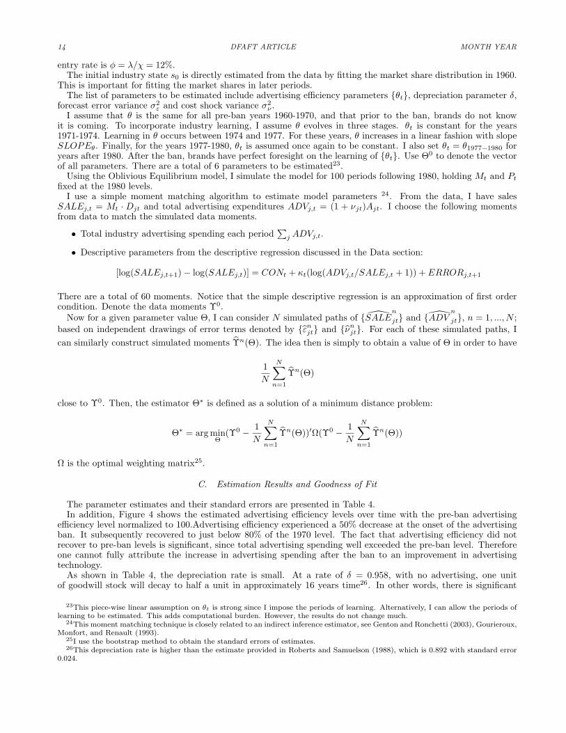
Figure 5 shows the goodness of fit to the total industry spending. The solid line represents the data, and thedotted line represents model prediction. The model fits the total industry spending levels in billions of (year 2000)dollars.

IV. Counterfactual Experiments

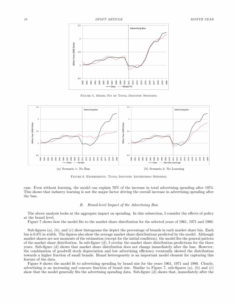
In this section, I contrast the estimated model with the following two experiments27. The first experiment is todetermine the evolution of the industry if there were no ban. I model this by assuming that advertising efficiencystays constant (θt = θ1960−1970 for all t = 1971, ..., 1980). The second experiment allows the ban, such thatefficiency drops after 1971. However, I do not allow advertising efficiency to recover in this experiment, so industrylearning is shut down (θt = θ1971−1974 for all t = 1971, ..., 1980).

Experiment (1) provides the baseline case to investigate the effects of the advertising ban. Specifically, it revealsthe impact of the ban on the overall increase in industry advertising spending, on brand heterogeneity and marketstructure, and on brand profitability. By comparing the estimated model to experiment (2), I show that industrylearning is not the major factor driving the overall increase in advertising spending after the ban.

A. Aggregate Advertising Spending

Figure 6 shows total industry advertising spending from the two above-mentioned experiments.As in Figure 5, the solid line in each sub-figure represents the data, while the dotted line represents model

prediction. In the first experiment, when there is no ban, the model predicts no significant shift in the trend oftotal advertising spending. This shows that the advertising ban and subsequent industry learning have contributedto the overall increase in advertising spending. In the second experiment, the industry cannot learn to improve itsadvertising efficiency level after the ban. The model predicts that advertising would experience an initial drop, butthen recover quickly. By the mid-1970s, total advertising spending in this case would exceed that in the no ban

27I do not re-estimate the model, but rather use the estimated parameter in these experiments.

16 DFAFT ARTICLE MONTH YEAR

1.5

2

2.5Advertising Ban

2000

Dollar

0.5

1

1960

1961

1962

1963

1964

1965

1966

1967

1968

1969

1970

1971

1972

1973

1974

1975

1976

1977

1978

1979

1980

Data Model Fit

Billion

Year

Figure 5. Model Fit of Total Industry Spending

1.5

2

2.5Advertising Ban

2000

Dollar

0.5

1

1960

1961

1962

1963

1964

1965

1966

1967

1968

1969

1970

1971

1972

1973

1974

1975

1976

1977

1978

1979

1980

Data No Ban

Billion

Year

(a) Scenario 1: No Ban

1.5

2

2.5Advertising Ban

2000

Dollar

0.5

1

1960

1961

1962

1963

1964

1965

1966

1967

1968

1969

1970

1971

1972

1973

1974

1975

1976

1977

1978

1979

1980

Data Ban (No Learning)

Billion

Year

(b) Scenario 2: No Learning

Figure 6. Experiments: Total Industry Advertising Spending

case. Even without learning, the model can explain 70% of the increase in total advertising spending after 1974.This shows that industry learning is not the major factor driving the overall increase in advertising spending afterthe ban.

B. Brand-level Impact of the Advertising Ban

The above analysis looks at the aggregate impact on spending. In this subsection, I consider the effects of policyat the brand level.

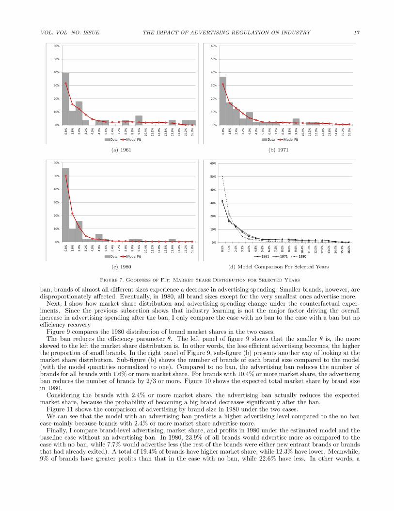
Figure 7 shows how the model fits to the market share distribution for the selected years of 1961, 1971 and 1980.

Sub-figures (a), (b), and (c) show histograms the depict the percentage of brands in each market share bin. Eachbin is 0.8% in width. The figures also show the average market share distributions predicted by the model. Althoughmarket shares are not moments of the estimation (except for the initial condition), the model fits the general patternof the market share distribution. In sub-figure (d), I overlay the market share distribution predictions for the threeyears. Sub-figure (d) shows that market share distribution does not change immediately after the ban. However,the combination of goodwill stock depreciation and low advertising efficiency eventually skewed the distributiontowards a higher fraction of small brands. Brand heterogeneity is an important model element for capturing thisfeature of the data.

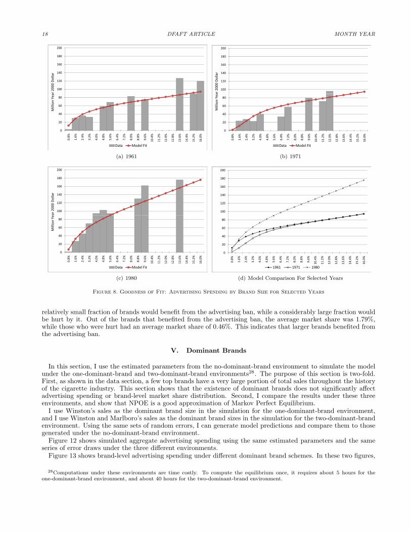
Figure 8 shows the model fit to advertising spending by brand size for the years 1961, 1971 and 1980. Clearly,advertising is an increasing and concave function of brand size. Similar to Figure 7, sub-figures (a), (b) and (c)show that the model generally fits the advertising spending data. Sub-figure (d) shows that, immediately after the

VOL. VOL NO. ISSUE THE IMPACT OF ADVERTISING REGULATION ON INDUSTRY 17

30%

40%

50%

60%

0%

10%

20%

0.8%

1.6%

2.4%

3.2%

4.0%

4.8%

5.6%

6.4%

7.2%

8.0%

8.8%

9.6%

10.4%

11.2%

12.0%

12.8%

13.6%

14.4%

15.2%

16.0%

Data Model Fit

(a) 1961

30%

40%

50%

60%

0%

10%

20%

0.8%

1.6%

2.4%

3.2%

4.0%

4.8%

5.6%

6.4%

7.2%

8.0%

8.8%

9.6%

10.4%

11.2%

12.0%

12.8%

13.6%

14.4%

15.2%

16.0%

Data Model Fit

(b) 1971

30%

40%

50%

60%

0%

10%

20%

0.8%

1.6%

2.4%

3.2%

4.0%

4.8%

5.6%

6.4%

7.2%

8.0%

8.8%

9.6%

10.4%

11.2%

12.0%

12.8%

13.6%

14.4%

15.2%

16.0%

Data Model Fit

(c) 1980

30%

40%

50%

60%

0%

10%

20%

0.8%

1.6%

2.4%

3.2%

4.0%

4.8%

5.6%

6.4%

7.2%

8.0%

8.8%

9.6%

10.4%

11.2%

12.0%

12.8%

13.6%

14.4%

15.2%

16.0%

1961 1971 1980

(d) Model Comparison For Selected Years

Figure 7. Goodness of Fit: Market Share Distribution for Selected Years

ban, brands of almost all different sizes experience a decrease in advertising spending. Smaller brands, however, aredisproportionately affected. Eventually, in 1980, all brand sizes except for the very smallest ones advertise more.

Next, I show how market share distribution and advertising spending change under the counterfactual exper-iments. Since the previous subsection shows that industry learning is not the major factor driving the overallincrease in advertising spending after the ban, I only compare the case with no ban to the case with a ban but noefficiency recovery

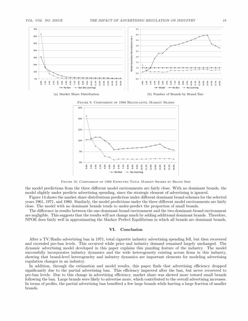
Figure 9 compares the 1980 distribution of brand market shares in the two cases.The ban reduces the efficiency parameter θ. The left panel of figure 9 shows that the smaller θ is, the more

skewed to the left the market share distribution is. In other words, the less efficient advertising becomes, the higherthe proportion of small brands. In the right panel of Figure 9, sub-figure (b) presents another way of looking at themarket share distribution. Sub-figure (b) shows the number of brands of each brand size compared to the model(with the model quantities normalized to one). Compared to no ban, the advertising ban reduces the number ofbrands for all brands with 1.6% or more market share. For brands with 10.4% or more market share, the advertisingban reduces the number of brands by 2/3 or more. Figure 10 shows the expected total market share by brand sizein 1980.

Considering the brands with 2.4% or more market share, the advertising ban actually reduces the expectedmarket share, because the probability of becoming a big brand decreases significantly after the ban.

Figure 11 shows the comparison of advertising by brand size in 1980 under the two cases.We can see that the model with an advertising ban predicts a higher advertising level compared to the no ban

case mainly because brands with 2.4% or more market share advertise more.Finally, I compare brand-level advertising, market share, and profits in 1980 under the estimated model and the

baseline case without an advertising ban. In 1980, 23.9% of all brands would advertise more as compared to thecase with no ban, while 7.7% would advertise less (the rest of the brands were either new entrant brands or brandsthat had already exited). A total of 19.4% of brands have higher market share, while 12.3% have lower. Meanwhile,9% of brands have greater profits than that in the case with no ban, while 22.6% have less. In other words, a

18 DFAFT ARTICLE MONTH YEAR

100

120

140

160

180

200r2

000 Dollar

0

20

40

60

80

0.8%

1.6%

2.4%

3.2%

4.0%

4.8%

5.6%

6.4%

7.2%

8.0%

8.8%

9.6%

10.4%

11.2%

12.0%

12.8%

13.6%

14.4%

15.2%

16.0%

Data Model Fit

Million Yea

(a) 1961

100

120

140

160

180

200

ar2000

Dollar

0

20

40

60

80

0.8%

1.6%

2.4%

3.2%

4.0%

4.8%

5.6%

6.4%

7.2%

8.0%

8.8%

9.6%

10.4%

11.2%

12.0%

12.8%

13.6%

14.4%

15.2%

16.0%

Data Model Fit

Million Yea

(b) 1971

100

120

140

160

180

200

ear2

000 Dollar

0

20

40

60

80

0.8%

1.6%

2.4%

3.2%

4.0%

4.8%

5.6%

6.4%

7.2%

8.0%

8.8%

9.6%

10.4%

11.2%

12.0%

12.8%

13.6%

14.4%

15.2%

16.0%

Data Model Fit

Million Ye

(c) 1980

100

120

140

160

180

200

0

20

40

60

80

0.8%

1.6%

2.4%

3.2%

4.0%

4.8%

5.6%

6.4%

7.2%

8.0%

8.8%

9.6%

10.4%

11.2%

12.0%

12.8%

13.6%

14.4%

15.2%

16.0%

1961 1971 1980

(d) Model Comparison For Selected Years

Figure 8. Goodness of Fit: Advertising Spending by Brand Size for Selected Years

relatively small fraction of brands would benefit from the advertising ban, while a considerably large fraction wouldbe hurt by it. Out of the brands that benefited from the advertising ban, the average market share was 1.79%,while those who were hurt had an average market share of 0.46%. This indicates that larger brands benefited fromthe advertising ban.

V. Dominant Brands

In this section, I use the estimated parameters from the no-dominant-brand environment to simulate the modelunder the one-dominant-brand and two-dominant-brand environments28. The purpose of this section is two-fold.First, as shown in the data section, a few top brands have a very large portion of total sales throughout the historyof the cigarette industry. This section shows that the existence of dominant brands does not significantly affectadvertising spending or brand-level market share distribution. Second, I compare the results under these threeenvironments, and show that NPOE is a good approximation of Markov Perfect Equilibrium.

I use Winston’s sales as the dominant brand size in the simulation for the one-dominant-brand environment,and I use Winston and Marlboro’s sales as the dominant brand sizes in the simulation for the two-dominant-brandenvironment. Using the same sets of random errors, I can generate model predictions and compare them to thosegenerated under the no-dominant-brand environment.

Figure 12 shows simulated aggregate advertising spending using the same estimated parameters and the sameseries of error draws under the three different environments.

Figure 13 shows brand-level advertising spending under different dominant brand schemes. In these two figures,

28Computations under these environments are time costly. To compute the equilibrium once, it requires about 5 hours for theone-dominant-brand environment, and about 40 hours for the two-dominant-brand environment.

VOL. VOL NO. ISSUE THE IMPACT OF ADVERTISING REGULATION ON INDUSTRY 19

40%

50%

60%

70%

0%

10%

20%

30%

0.8%

1.6%

2.4%

3.2%

4.0%

4.8%

5.6%

6.4%

7.2%

8.0%

8.8%

9.6%

10.4%

11.2%

12.0%

12.8%

13.6%

14.4%

15.2%

16.0%

No Ban Ban (No Learning)

(a) Market Share Distribution

2 0

2.5

3.0

3.5

4.0

4.5

es Normalized

to be 1

0.0

0.5

1.0

1.5

2.0

0.8%

1.6%

2.4%

3.2%

4.0%

4.8%

5.6%

6.4%

7.2%

8.0%

8.8%

9.6%

10.4%

11.2%

12.0%

12.8%

13.6%

14.4%

15.2%

16.0%

Model No Ban No Learning

Mod

el Quantitie

(b) Number of Brands by Brand Size

Figure 9. Comparison of 1980 Brand-level Market Shares

15%

20%

25%

0%

5%

10%

0.8%

1.6%

2.4%

3.2%

4.0%

4.8%

5.6%

6.4%

7.2%

8.0%

8.8%

9.6%

10.4%

11.2%

12.0%

12.8%

13.6%

14.4%

15.2%

16.0%

No Ban No Learning

Figure 10. Comparison of 1980 Expected Total Market Shares by Brand Size

the model predictions from the three different model environments are fairly close. With no dominant brands, themodel slightly under predicts advertising spending, since the strategic element of advertising is ignored.

Figure 14 shows the market share distributions prediction under different dominant brand schemes for the selectedyears 1961, 1971, and 1980. Similarly, the model predictions under the three different model environments are fairlyclose. The model with no dominant brands tends to under-predict the proportion of small brands.

The difference in results between the one-dominant-brand environment and the two-dominant-brand environmentare negligible. This suggests that the results will not change much by adding additional dominant brands. Therefore,NPOE does fairly well in approximating the Markov Perfect Equilibrium in which all brands are dominant brands.

VI. Conclusion

After a TV/Radio advertising ban in 1971, total cigarette industry advertising spending fell, but then recoveredand exceeded pre-ban levels. This occurred while price and industry demand remained largely unchanged. Thedynamic advertising model developed in this paper explains this puzzling feature of the industry. The modelsuccessfully incorporates industry dynamics and the wide heterogeneity existing across firms in this industry,showing that brand-level heterogeneity and industry dynamics are important elements for modeling advertisingregulation changes in an industry.

In addition, through the estimation and model results, this paper finds that advertising efficiency droppedsignificantly due to the partial advertising ban. This efficiency improved after the ban, but never recovered topre-ban levels. Due to this change in advertising efficiency, market share was skewed more toward small brandsfollowing the ban. Large brands were likely to advertise more, which contributed to the overall advertising increases.In terms of profits, the partial advertising ban benefited a few large brands while hurting a large fraction of smallerbrands.

20 DFAFT ARTICLE MONTH YEAR

150

200

250

Year

2000

Dollar

0

50

100

0.8%

1.6%

2.4%

3.2%

4.0%

4.8%

5.6%

6.4%

7.2%

8.0%

8.8%

9.6%

10.4%

11.2%

12.0%

12.8%

13.6%

14.4%

15.2%

16.0%

No Ban Ban (No Learning)

Million Y

Figure 11. Comparison of 1980 Advertising by Size of Brands

1.5

2

2.5

ear2

000 Dollar

0

0.5

1

0.8%

1.6%

2.4%

3.2%

4.0%

4.8%

5.6%

6.4%

7.2%

8.0%

8.8%

9.6%

10.4%

11.2%

12.0%

12.8%

13.6%

14.4%

15.2%

16.0%

No DOM One DOM Two DOM

Billion

Ye

Figure 12. Aggregate Advertising Spending Under Different Dominant Brand Environments

In future research, I plan to incorporate strategic entry and exit, and consider coordination in advertisingdecisions among brands of the same company.

REFERENCES

Alonso, R., W. Dessein, and N. Matouschek. “When Does Coordination Require Centralization.” AmericanEconomic Review forthcoming.

Bagwell, K. “The Economic Analysis of Advertising.” Working Paper .

Bajari, P., C.L. Benkard, and J. Levin. “Estimating Dynamic Models of Imperfect Competition.” Econometrica75, 5: (2007) 1331–1370.

Benkard, C.L. “A Dynamic Analysis of the Market for Wide-Bodied Commercial Aircraft.” The Review of EconomicStudies 71, 3: (2004) 581–611.

Berry, S., J. Levinsohn, and A. Pakes. “Automobile Prices in Market Equilbrium.” Econometrica 63, 4: (1995)841–890.

Carter, S. M. “Tobacco Document Research Reporting.” Tobacco Control 14: (2007) 368–376.

Doraszelski, U., and S. Markovich. “Foundation of Markov-perfect Industry Dynamics: Existence, Purification andMultiplicity.” Working Paper .

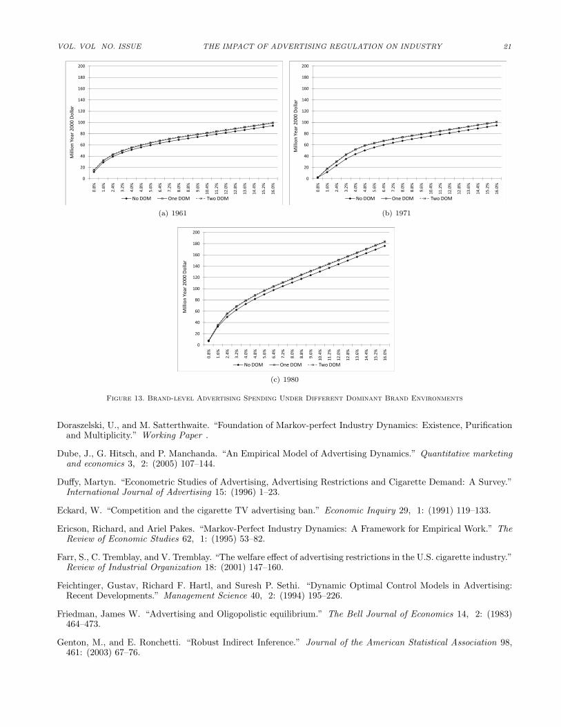
VOL. VOL NO. ISSUE THE IMPACT OF ADVERTISING REGULATION ON INDUSTRY 21

100

120

140

160

180

200000 Dollar

0

20

40

60

80

0.8%

1.6%

2.4%

3.2%

4.0%

4.8%

5.6%

6.4%

7.2%

8.0%

8.8%

9.6%

10.4%

11.2%

12.0%

12.8%

13.6%

14.4%

15.2%

16.0%

No DOM One DOM Two DOM

Million Year

20

(a) 1961

100

120

140

160

180

200

r2000 Dollar

0

20

40

60

80

0.8%

1.6%

2.4%

3.2%

4.0%

4.8%

5.6%

6.4%

7.2%

8.0%

8.8%

9.6%

10.4%

11.2%

12.0%

12.8%

13.6%

14.4%

15.2%

16.0%

No DOM One DOM Two DOM

Million Yea

(b) 1971

100

120

140

160

180

200

ear2

000 Dollar

0

20

40

60

80

0.8%

1.6%

2.4%

3.2%

4.0%

4.8%

5.6%

6.4%

7.2%

8.0%

8.8%

9.6%

10.4%

11.2%

12.0%

12.8%

13.6%

14.4%

15.2%

16.0%

No DOM One DOM Two DOM

Million Y

(c) 1980

Figure 13. Brand-level Advertising Spending Under Different Dominant Brand Environments

Doraszelski, U., and M. Satterthwaite. “Foundation of Markov-perfect Industry Dynamics: Existence, Purificationand Multiplicity.” Working Paper .

Dube, J., G. Hitsch, and P. Manchanda. “An Empirical Model of Advertising Dynamics.” Quantitative marketingand economics 3, 2: (2005) 107–144.

Duffy, Martyn. “Econometric Studies of Advertising, Advertising Restrictions and Cigarette Demand: A Survey.”International Journal of Advertising 15: (1996) 1–23.

Eckard, W. “Competition and the cigarette TV advertising ban.” Economic Inquiry 29, 1: (1991) 119–133.

Ericson, Richard, and Ariel Pakes. “Markov-Perfect Industry Dynamics: A Framework for Empirical Work.” TheReview of Economic Studies 62, 1: (1995) 53–82.

Farr, S., C. Tremblay, and V. Tremblay. “The welfare effect of advertising restrictions in the U.S. cigarette industry.”Review of Industrial Organization 18: (2001) 147–160.

Feichtinger, Gustav, Richard F. Hartl, and Suresh P. Sethi. “Dynamic Optimal Control Models in Advertising:Recent Developments.” Management Science 40, 2: (1994) 195–226.

Friedman, James W. “Advertising and Oligopolistic equilibrium.” The Bell Journal of Economics 14, 2: (1983)464–473.

Genton, M., and E. Ronchetti. “Robust Indirect Inference.” Journal of the American Statistical Association 98,461: (2003) 67–76.

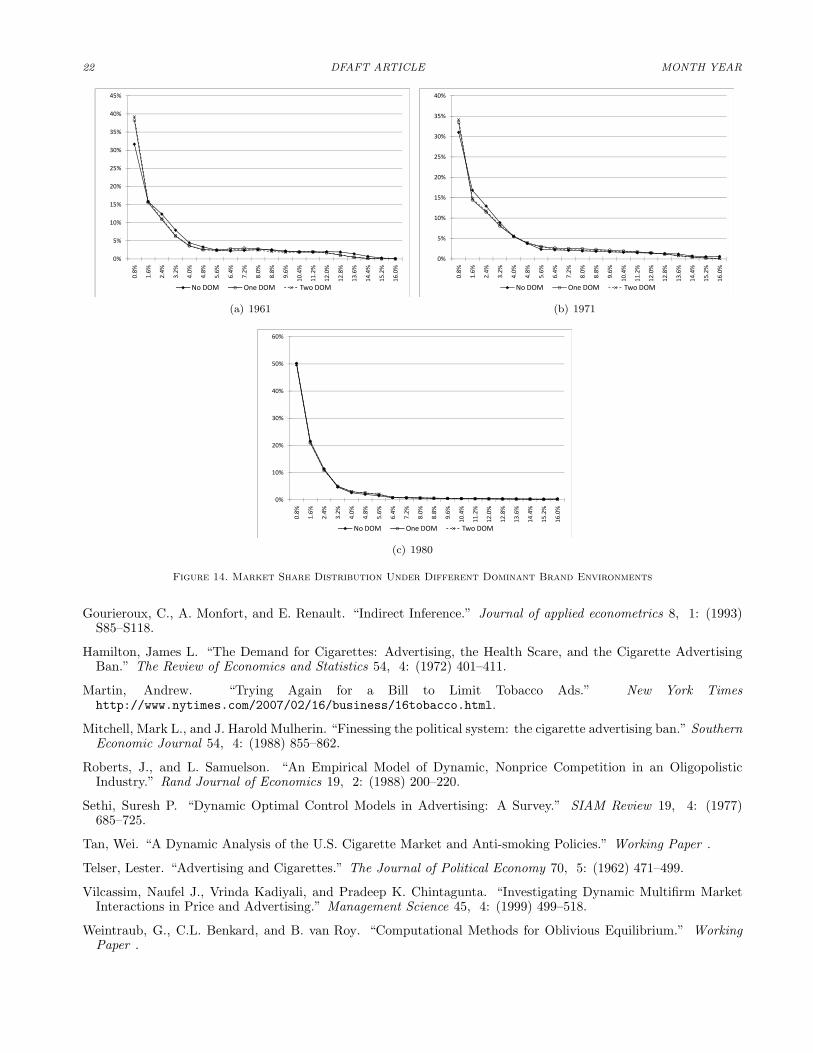
22 DFAFT ARTICLE MONTH YEAR

20%

25%

30%

35%

40%

45%

0%

5%

10%

15%

20%

0.8%

1.6%

2.4%

3.2%

4.0%

4.8%

5.6%

6.4%

7.2%

8.0%

8.8%

9.6%

10.4%

11.2%

12.0%

12.8%

13.6%

14.4%

15.2%

16.0%

No DOM One DOM Two DOM

(a) 1961

20%

25%

30%

35%

40%

0%

5%

10%

15%

0.8%

1.6%

2.4%

3.2%

4.0%

4.8%

5.6%

6.4%

7.2%

8.0%

8.8%

9.6%

10.4%

11.2%

12.0%

12.8%

13.6%

14.4%

15.2%

16.0%

No DOM One DOM Two DOM

(b) 1971

30%

40%

50%

60%

0%

10%

20%

0.8%

1.6%

2.4%

3.2%

4.0%

4.8%

5.6%

6.4%

7.2%

8.0%

8.8%

9.6%

10.4%

11.2%

12.0%

12.8%

13.6%

14.4%

15.2%

16.0%

No DOM One DOM Two DOM

(c) 1980

Figure 14. Market Share Distribution Under Different Dominant Brand Environments

Gourieroux, C., A. Monfort, and E. Renault. “Indirect Inference.” Journal of applied econometrics 8, 1: (1993)S85–S118.

Hamilton, James L. “The Demand for Cigarettes: Advertising, the Health Scare, and the Cigarette AdvertisingBan.” The Review of Economics and Statistics 54, 4: (1972) 401–411.

Martin, Andrew. “Trying Again for a Bill to Limit Tobacco Ads.” New York Timeshttp://www.nytimes.com/2007/02/16/business/16tobacco.html.

Mitchell, Mark L., and J. Harold Mulherin. “Finessing the political system: the cigarette advertising ban.” SouthernEconomic Journal 54, 4: (1988) 855–862.

Roberts, J., and L. Samuelson. “An Empirical Model of Dynamic, Nonprice Competition in an OligopolisticIndustry.” Rand Journal of Economics 19, 2: (1988) 200–220.

Sethi, Suresh P. “Dynamic Optimal Control Models in Advertising: A Survey.” SIAM Review 19, 4: (1977)685–725.

Tan, Wei. “A Dynamic Analysis of the U.S. Cigarette Market and Anti-smoking Policies.” Working Paper .

Telser, Lester. “Advertising and Cigarettes.” The Journal of Political Economy 70, 5: (1962) 471–499.

Vilcassim, Naufel J., Vrinda Kadiyali, and Pradeep K. Chintagunta. “Investigating Dynamic Multifirm MarketInteractions in Price and Advertising.” Management Science 45, 4: (1999) 499–518.

Weintraub, G., C.L. Benkard, and B. van Roy. “Computational Methods for Oblivious Equilibrium.” WorkingPaper .

VOL. VOL NO. ISSUE THE IMPACT OF ADVERTISING REGULATION ON INDUSTRY 23

. “Extensions to Oblivious Equilibrium.” Working Paper .

. “Markov Perfect Industry Dynamics with Many Firms.” Working Paper .

———————–Appendix: Not for Publication————————————

Mathematical Appendix

Expected Fringe Brand State

For convenience, denote zt(s, w) to be the s component of z(σ,y0,z0),t(w)). Here I assume w = y for simplicity.Under strategy profile σ, I denote the probability of the dominant states being y in time period t to be Πt(y|σ),

and denote the probability of dominant brands transition from state y′ in period t−1 to y in period t given they usestrategy σ to be ρdom

t (y|y′, σ), where ρdomt (y|y′, σ) is the product of all dominant brands’ transition probabilities.

Then, the following relationships hold:

Πt+1(y|σ) =∫

y′Πt(y′|σ) dρdom

t (y|y′, σ)(7)

where Π0(y0) = 1, and Π0(y) = 0 for all y 6= y0. Given the definition the Π, I define ζt(s, y) = zt(s, y)Πt(y), then:

ζt+1(s, y) =∫

s′

∫y′ζt(s

′, y′) dρdomt (y|y′, σ) dρt(s|s′, σ) + λρe(s)Πt(y)(8)

where ρe(s) is probability of entrant brand obtaining state s in its initial period. Given equation (7) and equation(8), I can obtain z(σ,y0,z0),t(y) and Πt(y|σ) iteratively.

Transition Probability

Here I show the transition function for a more general case than the one shown in the main part of the paper.Slightly modify equation (5) and use the following notation:

s∗j,t+1 = δsjt + f(Ajt)sj,t+1 = s∗j,t+1 + εj,t+1

s is continuous, and sj,t+1 is discretized into sj,t+1. And consider the discretized state space g ∈ g0, ..., gL, wheregk − gk−1 = d for all k (For the paper, g0 = 0 and d = 1).

Similar to Benkard (2004), I use a binomial random variable to specify the period t+1 goodwill level sj,t+1. Forany given ε, the probability of sj,t+1 = gk is:

Pr(gk|s, ε) =

s−gk−1gk−gk−1

if gk−1 ≤ s < gk

1− s−gk

gk+1−gkif gk ≤ s < gk+1

0 otherwise

For the period t + 1 the probability of next period’s state to be any gk, and for s∗ defined by above equations,

24 DFAFT ARTICLE MONTH YEAR

given any s and A:

ρt(gk|s,A) =

∫

ε∈Ωk−1[(s∗ − gk−1 + ε)/d] dΦ(ε) +

∫ε∈Ωk

[1− (s∗ − gk + ε)/d] dΦ(ε) if k ∈ (0, L)Φ(g0 − s∗) +

∫ε∈Ω0

[1− (s∗ − g0 + ε)/d] dΦ(ε) if k = 01− Φ(gL − s∗) +

∫ε∈ΩL−1

[(s∗ − gL−1 + ε)/d] dΦ(ε) if k = L

where Ωk = [gk − s∗, gk+1 − s∗).

Existence of Optimal Advertising Solution

Here I only consider the solution for Oblivious Equilibrium under no-dominant firms. So it is sufficient to consideronly one representative firm. From equation (2), the first order necessary condition is

−(k + νjt) + β ·∑

k

Wj,t+1(gk)∂ρt(gk|s,A)

∂A= 0

Recall Leibniz Rule:∂

∂z

∫ b(z)

a(z)

f(x)dx = f(b(z))∂b

∂z− f(a(z))

∂a

∂z

Recall from above the probability transition function, let ϕ(·) be the pdf of ε distribution then:

∂ρt(gk|s,A)∂A

=∂s∗

∂A

1d·[Φ(ε)|Ωk−1 − Φ(ε)|Ωk

]=∂s∗

∂A

1d[2Φ(gk − s∗)− Φ(gk−1 − s∗)− Φ(gk+1 − s∗)]

∂ρt(g0|s,A)∂A

= −∂s∗

∂A

1d· Φ(ε)|Ω0 =

∂s∗

∂A

1d· (Φ(g0 − s∗)− Φ(g1 − s∗))

∂ρt(gL|s,A)∂A

=∂s∗

∂A

1d· Φ(ε)|ΩL−1 =

∂s∗

∂A

1d· (Φ(gL − s∗)− Φ(gN−1 − s∗))

where:∂s∗

∂A=

θt

θtA+ 1Check second order condition, and need: SOC of A to satisfy the following to ensure concavity and solution.

β∑

k

Wj,t+1(gk)∂2ρt(gk|s,A)

∂A2< 0

It’s clear from above that:

∂2ρt(gk|s,A)∂A2

=∂2s∗

∂A2

1d[2Φ(gk − s∗)− Φ(gk−1 − s∗)− Φ(gk+1 − s∗)]

−(∂s∗

∂A

)2 1d[2ϕ(gk − s∗)− ϕ(gk−1 − s∗)− ϕ(gk+1 − s∗)]

Similarly define ∂2ρt(g0|s,A)∂A2 and ∂ρt(gL|s,A)

∂A . Simplify notation a bit, let’s call Φ(gk − s∗)−Φ(gk−1 − s∗) = Φk, andcall ϕ(gk − s∗)− ϕ(gk−1 − s∗) = ϕk, let the following be defined:

Cm1 = −W0 · Φ1 + (W1Φ1 −W1Φ2) + ...+ (WL−1ΦL−1 −WL−1ΦL) +WLΦL

= (W1 −W0)Φ1 + (W2 −W1)Φ2 + ...+ (WL −WL−1)ΦL

Cm2 = −W0 · ϕ1 + (W1ϕ1 −W1ϕ2) + ...+ (WL−1ϕL−1 −WL−1ϕL) +WLϕL

= (W1 −W0)ϕ1 + (W2 −W1)ϕ2 + ...+ (WL −WL−1)ϕL

VOL. VOL NO. ISSUE THE IMPACT OF ADVERTISING REGULATION ON INDUSTRY 25

Then, the second order condition looks like:

β

d·

(∂2s∗

∂A2· Cm1 −

(∂s∗

∂A

)2

· Cm2

)

By assumption that η ∈ (0, 1), W is concave in goodwill stock, then Wk > Wk−1. Due to the nature of CDF of adistribution, I know that Cm1 > 0. Also by assumption, I know ∂2s∗

∂A2 < 0. Furthermore:

∂2s∗

∂A2= − θ2t

(θtAjt + 1)2(∂s∗

∂A

)2

=(

θt

θtAjt + 1

)2

then it is clear that |∂2s∗

∂A2 | =(

∂s∗

∂A

)2

, then it is clear that as A increases, at s = s∗ the value function becomesconcave. Therefore, the problem has a solution.

A Myopic Example of Advertising Spending Recovery

To illustrate the intuition behind the advertising spending recovery, consider a simple example of the modelpresent in the paper. In this example, all firms are assumed to be myopic, or β = 0; ignore both forecast error εand brand cost shock ν; the number of brand is fixed at N and there is no entry or exit; and assume all brandsare symmetric.

I use this example to illustrate that in steady states, when advertising efficiency parameter θ decreases, threethings can happen for a representative firm: (1) long run steady state goodwill stock decreases; (2) long run steadystate advertising spending increases; (3) when transition from a steady state with high θ to a steady state withlow θ, advertising spending initially falls then recovers.

Let advertising of firm j be Ajt. Let goodwill be sjt. Suppose s evolves in the following fashion:

sj,t = δsjt−1 + log(θtAjt + 1)

Let Ds(A) denote the derivative of s with respect to A, then Ds(A) = θθA+1 . And assume the revenue for each

individual is just its market share:

Rj =sj∑Ji=1 si

= 1−∑

i 6=j si + 1∑i(si + 1)

The specifications above are the same as in the paper. Then, a firm j in time t solve the following problem:

maxA

Rj(A)−A

And the first order necessary condition is:

Dsj(Aj) ·∑

i 6=j si + 1

(∑

i(si + 1))2− 1 = 0

Suppose that we have a symmetric equilibrium where all firms have goodwill stock level st (this is possible whenall firms start with the same initial state), then since the number of firms is N :

N − 1N2

θθAt+1

st + 1− 1 = 0

Suppose in steady state, and st = s∗ At = A∗ for all t, then:

s∗ =log(θA∗ + 1)

1− δ

26 DFAFT ARTICLE MONTH YEAR

then the first order condition is:

N − 1N2

1− δ

log(θA∗ + 1) + (1− δ)θ

θA∗ + 1− 1 = 0

The above two equations give the long run steady state goodwill stock s∗ and advertising spending A∗ as functionsof advertising efficiency θ. To see how A∗ changes with respect to θ, I consider the elasticity term θDA(θ)/A(θ). Ican totally differentiate the first order condition to get this:

θDA∗(θ)A∗(θ)

=1

(1 + [log(θA∗ + 1) + (1− δ)]−1)θA∗ + 1θA∗ − 1

Denote ς(θA∗(θ)) = (1 + [log(θA∗ + 1) + (1 − δ)]−1) θA∗

θA∗+1 . Notice that ς(x) = −xD2R(x)DR(x) . Hence if the curvature

of revenue function is large, or ς(x) > 1, then an increase in θ leads to decrease in A∗. Since the revenue functionis asymptotically converging to a finite number, when θ is large enough, ς(x) > 1.

2

2.5

3

A(5)=1

0.5

1

1.5

5 15 25 35 45 55 65 75 85 95 105

Normalized

θ

(a) Steady State Advertising A∗

15

20

25

s(5)=1

0

5

10

5 15 25 35 45 55 65 75 85 95 105

Normalized

θ

(b) Steady State Goodwill Stock s∗

Figure A.1. Simple Example: A∗ and s∗ as functions of θSince it is difficult to get analytical results from the above expressions, I use the following numerical example to

illustrate the intuition. I choose N = 3, δ = 0.8, and let θ varying on the interval [5, 105], with grid size 1 (for awide range of parameters, the qualitative results hold). I show functions A∗(θ) and s∗(θ) in Figure A.1. As show,as θ increases, the steady state advertising A∗ increases initially, then decreases steadily after attaining a max levelaround θ = 30. In addition, I show the steady state transition when θ is lowered from 150 to 30 in Figure A.2.Advertising spending initially drops but recovers quickly to the new steady state, which is higher than the initial

80

100

120

140

Period 0=100

0

20

40

60

0 1 2 3 4 5 6 7 8 9 10 11 12 13 14 15 16 17 18 19 20

Normalized

t

(a) Advertising A

60

80

100

120

Period 0=100

0

20

40

0 1 2 3 4 5 6 7 8 9 10 11 12 13 14 15 16 17 18 19 20

Normalized

t

(b) Goodwill Stock s

Figure A.2. Simple Example: Steady State Transition

level. Meantime, we see a downward adjustment in goodwill stock level. The initial drop of advertising spending

VOL. VOL NO. ISSUE THE IMPACT OF ADVERTISING REGULATION ON INDUSTRY 27

was due to lack of immediate change in goodwill stock level.