the hydrodynamical models ofthe cometary compact h iiregion · feng-yao zhu1,2, qing-feng zhu1,2,...
TRANSCRIPT
arX
iv:1
510.
0318
3v1
[as
tro-
ph.S
R]
12
Oct
201
5
The hydrodynamical models of the cometary compact H II region
Feng-Yao Zhu1,2, Qing-Feng Zhu1,2, Juan Li3, Jiang-Shui Zhang4 and Jun-Zhi Wang5
ABSTRACT
We have developed a full numerical method to study the gas dynamics of cometary ultra-
compact (UC) H II regions, and associated photodissociation regions (PDRs). The bow-shock
and champagne-flow models with a 40.9/21.9 M⊙ star are simulated. In the bow-shock models,
the massive star is assumed to move through dense (n = 8000 cm−3) molecular material with
a stellar velocity of 15 km s−1. In the champagne-flow models, an exponential distribution of
density with a scale height of 0.2 pc is assumed. The profiles of the [Ne II] 12.81µm and H2 S(2)
lines from the ionized regions and PDRs are compared for two sets of models. In champagne-
flow models, emission lines from the ionized gas clearly show the effect of acceleration along the
direction toward the tail due to the density gradient. The kinematics of the molecular gas inside
the dense shell is mainly due to the expansion of the H II region. However, in bow-shock models
the ionized gas mainly moves in the same direction as the stellar motion. The kinematics of the
molecular gas inside the dense shell simply reflects the motion of the dense shell with respect to
the star. These differences can be used to distinguish two sets of models.
Subject headings: H II regions — ISM: molecules — ISM: kinematics and dynamics — line:
profiles
1. Introduction
Massive stars are always formed in dense molecular clouds, and the feedback processes of these stars can
affect the surrounding interstellar medium (ISM) significantly. When a massive star is born, the surrounding
neutral ISM begins to be ionized by stellar EUV (hυ ≥ 13.6 eV ) radiation and an H II region is formed.
The over-pressurized ionized gas in the H II region will expand and compress the nearby neutral gas. The
materials around the H II region are swept up by the expanding H II region to form a dense shell containing
mainly neutral gases (Tenorio-Tagle 1979; Mac Low et al. 1991). Outside of the photoionized region, the
molecular gas is dissociated by FUV radiation (11.26 eV ≤ hυ < 13.6 eV ) to form a photodissociation region
(PDR). The temperature of the neutral gas in PDR ranges from ∼ 3000 K (close to the ionized region) to
∼ 100 K (Spitzer 1978; Roger & Dewdney 1992). Besides the stellar radiation, stellar winds also have a
significant impact on the ISM. The high-velocity outflowing wind from massive stars is embedded in the
photoionized region and interacts with the ionized gas. The photoionized gas decelerates the stellar wind
so that the kinetic energy of the stellar wind is converted into thermal energy. A hot low-density bubble
1Astronomy Department, University of Science and Technology of China, Hefei, China 230026, [email protected]
2Key Laboratory for Research in Galaxies and Cosmology, University of Science and Technology of China, Chinese Academy
of Sciences, Hefei, China, 230026
3Shanghai Astronomical Observatory, Chinese Academy of Sciences, Shanghai, China
4Center for Astrophysics, Guangzhou University, Guangzhou, China
5Shanghai Astronomical Observatory, Chinese Academy of Sciences, Shanghai, China

– 2 –
composed of stellar wind material (T ≥ 106 K, n ≤ 5 cm−3) with a surrounding shell of swept-up ionized
gas is produced. The kinetic and thermal energy of the stellar-wind bubble can increase the expansion of
the H II region (Comeron 1997).
If the expansion of H II regions are envisaged in a uniform environment, a spherical H II region results and
its evolution is well described by the Stromgren sphere model (Stromgren 1939). However, a large fraction
(∼ 20%) of young H II regions are not spherical, but have a cometary morphology (Wood & Churchwell
1989; Kurtz et al. 1994; Walsh et al. 1998). The study of the formation of such a morphology can improve
our understanding of the interaction between massive stars and the interstellar medium. In order to explain
this morphology, two kinds of models, champagne-flow models and bow-shock models, are suggested. The
champagne-flow model was first suggested by Tenorio-Tagle (1979), and further improved by including
stellar wind, various ambient density distributions and magnetic fields (Yorke et al. 1983; Comeron 1997;
Arthur & Hoare 2006; Gendelev & Krumholz 2012). The main characteristic of these models is that density
gradients in the molecular cloud result in the anisotropic expansion of the H II region and thence the cometary
morphology. The Orion Nebula is the archetype of this kind of H II region (Israel 1978; Tenorio-Tagle 1979).
Observations of the nebula show that there is a bright ionization front on the surface of a molecular cloud
and ionized gas flows away from the cloud in the opposite direction. There are also a series of bow-shock
models (Mac Low et al. 1991; van Buren & Mac Low 1992; Comeron & Kaper 1998; Arthur & Hoare 2006;
Mackey et al. 2015). The key point of these models is that the supersonic movement of a wind-blowing
massive star relative to the molecular cloud causes the ionization front to be trapped in a dense cometary
shell which is behind the bow shock ahead of the star.
In order for the champagne-flow models to work, a density gradient must exist around the newly
formed star. Density gradients seem to be unavoidable in the realistic environment of the molecular cloud
(Kleinmann et al. 1977; Schneps et al. 1978; Arquilla & Goldsmith 1984). Observations show that the molec-
ular clouds are centrally condensed. The density gradients are approximated by power laws ρ(r) ∝ r−α in
some previous works (Arquilla & Goldsmith 1985; Hatchell & van der Tak 2003; Franco et al. 2000). Evi-
dence of various power indices from 1.6 to 2.5 is found by different authors (Pirogov 2009; Sano et al. 2010).
Some evidences suggest a steeper index in the outer parts of dense cores (eg., 3.9 in Hung et al. (2010)).
Since the density does not go to infinity at the center, a simple power law is combined with an exponential
law in Franco et al. (2007). It is very likely that stars form at the center of the cores and is surrounded by
non-uniform halos. In the current work, an exponential density distribution with a scale height of 0.2 pc
is used in our champagne-flow models. Such a distribution is not very different from a power law with an
index of 3.
For bow-shock models, a UV photon emitting star moving supersonically with respect to a molecular
cloud is needed. High velocity massive stars could be present in massive star-forming regions (Jones & Walker
1988). Stars could have a modest initial velocity (2 − 5 km s−1) due to the turbulent dynamics of their
parental clouds (McKee & Ostriker 2007; Peters et al. 2010). Binary interactions allow particular massive
stars to obtain more substantial velocities (∼ 30 km s−1) (Hoogerwerf et al. 2001). The temperatures in H
II regions are typically Ti ≈ 104 K, and the corresponding sound speeds are ai ≈ 13 km s−1. If the stellar
velocity is v∗ > ai, there will be a stellar wind bow shock formed in the H II region. And for a subsonic
stellar velocity with respect to the H II region, no stellar wind bow shock will form in the photoionized
region (Baranov et al. 1971; Mackey et al. 2015).
The PDR is important to the kinematics and radiation transfer of the entire region. Most of the high-
energy photons emitted from massive stars are absorbed in PDRs and converted into low-energy photons.
Moreover, the dynamical structure and expansion of the H II region are also influenced by the distribution

– 3 –
of the neutral gas. At the same time, the development of H II regions also affects the kinematics and
morphology of the neutral gas. These should be reflected in the line emission. The study of the dynamical
structure of the neutral gas is therefore an important complement to the study of H II regions. To complete
our picture about massive star formation, a hydrodynamical model including details both in ionized regions
and PDRs is necessary. Although many champagne-flow and bow-shock models have been studied, there
are only a few models including detailed thermal and dynamical processes both in the ionized region and
the PDR. In most models, the heating by dissociating photons is neglected. When calculating the cooling
in the PDR, it is assumed that hydrogen and oxygen are atomic meanwhile carbon is maintained in the
singly ionized stage by FUV photons. This assumption is appropriate if the ISM is low-density because
the timescales for the dissociation of H2 and CO are very short (< 100 yr), and the low density prevents
the molecules from reformation. However, if the density is as high as n ∼ 105 cm−3 in the shell of H II
regions, the timescales for dissociations and reformations of H2 and CO could be both ∼ 10, 000 yr, and this
method will overestimate cooling rates because the real fractional abundances of H , O and C+ are lower
than assumed. In order to get more accurate cooling rates, the accurate fractional abundances of different
components in the PDR should be calculated. The heating processes in the PDR also need to be included.
In the current work, we try to develop a new model including detailed processes both in the H II region
and the PDR to obtain a more complete picture of cometary compact H II regions. The dynamics of the gas
in the PDR is also included in the hydrodynamic simulation. The heating and cooling processes in the PDR
are treated once the fractional abundances are calculated. After completing the hydrodynamic simulation,
the [Ne II] 12.81 µm line and the H2 S(2) J = 4 − 2 12.28 µm rotational line are selected to depict the
gas motions in the H II region and the PDR, respectively. These two lines are both in the mid-infrared
and can be accessed by Stratospheric Observatory for Infrared Astronomy (SOFIA). We also investigate the
possibilities of using these mid-infrared lines to discriminate between bow shocks and champagne flows. For
this purpose, the profiles and position-velocity diagrams of these lines from bow-shock and champagne-flow
models are compared.
The organization of the current work is as follows: In §2 we explain our numerical method used in
simulations. We present the results of models and the discussions in §3. Our conclusions are presented in
§4.
2. Numerical Mehthod
We investigate the evolution of the cometary H II region around a newly formed massive star together
with the surrounding PDR. In our simulations, the coupled hydrodynamics and the radiative transfer equa-
tions are solved at the same time. Gravity and magnetic fields are neglected.
2.1. Hydrodynamics
The dynamical evolution of the H II region and the PDR is treated with a 2D explicit Eulerian method
in cylindrical coordinates. The models in this paper are all computed on a 250×500 grid. Due to the various
sizes of the cometary H II regions in different models, the cell size of the grids in champagne-flow models is
chosen to be 0.005 pc, and that in bow-shock models is 0.0025 pc. The equations of hydrodynamics are as
follows,

– 4 –
∂ρ
∂t= −
∂ρvr∂r
−∂ρvz∂z
−ρvrr
(1)
∂ρvr∂t
= −∂(ρv2r + p)
∂r−
∂ρvrvz∂z
−ρv2rr
(2)
∂ρvz∂t
= −∂ρvrvz∂r
−∂(ρv2z + p)
∂z−
ρvrvzr
(3)
∂Et
∂t= −
∂(Et + p)vr∂r
−∂(Et + p)vz
∂z−
(Et + p)vrr
(4)
where r and z are the radial and axial coordinates, respectively; ρ is the density; vr and vz are the
radial and axial components of velocity; p is the pressure, and Et is the total energy density as the sum of
the kinetic and thermal energy densities.
These hydrodynamical equations are solved by using a hybrid scheme combining a HLLC Riemann
solver (Miyoshi & Kusano 2005) and a NND-1 scheme (Zhang & Shen 2003; Zhu et al. 1996). The NND-1
scheme smoothes the oscillations. The stellar wind with a mass-loss rate M and a terminal velocity vw is
treated as a volume-distributed source of mass and energy (Rozyczka 1985; Comeron 1997; Arthur & Hoare
2006). The mass-loss rates and terminal velocities of stellar winds are obtained from the analytic formulae
given in Dale et al. (2013). After calculating the hydrodynamic evolution in a computational step, the effects
of heating and cooling processes are added explicitly. The energy density is updated with the corresponding
heating/cooling rates and the time for the step, which is the minimum of the hydrodynamic time given by
Courant-Friedrichs-Lewy condition and the cooling time (Arthur & Henney 1996).
2.2. the Radiative Transfer
In our simulation, the central star is the single source for radiation. The radiative transfer of the
ionizing EUV radiation (hυ ≥ 13.6 eV ) and the dissociating FUV radiation (11.26 eV ≤ hυ < 13.6 eV )
is solved separately. We use the frequency-integrated EUV and FUV photon luminosities of ionizing stars
provided by Diaz-Miller et al. (1998). The spectra of the stars are assumed to be black-body. The solar
abundances are assumed for all the models in this work (Hollenbach & McKee 1989). In the ionized region,
if the local ionizing photon flux is higher than 1010 cm−2 s−1, ionization equilibrium is adopted. And if the
local photons flux is low, the photoionization and recombination are time dependent. The equations for the
time-dependent photoionization and recombination in the ionized region are as follow,
∂nH+
∂t= nHσEUV FEUV − αn2
H+ −∂nH+vr
∂r−
∂nH+vz∂z
−nH+vr
r(5)
∂nH
∂t= −nHσEUV FEUV + αn2
H+ −∂nHvr∂r
−∂nHvz∂z
−nHvrr
(6)
where nH+ and nH are number densities of ionized hydrogen and atomic hydrogen, respectively. σEUV
and α are the absorption and recombination coefficients, and FEUV is the flux of EUV photons. In the H

– 5 –
II region, we consider the photoionization heating as the only heating process (Spitzer 1978). The ”on the
spot” approximation is assumed in treating ionizing photons. We use the empirical cooling curve for gas
with solar abundances given by Mellema & Lundqvist (2002) who consider the cooling due to the collisional
excitation of hydrogen and metal atoms and the recombination radiation of hydrogen atoms.
For the PDR, photoelectric heating, heating from photodissociation, reformation of and FUV pump-
ing of H2 molecules, and cosmic rays are considered in the simulations as heating processes of the gas.
Cooling processes considered include atomic fine-structure line emission of [O I] 63µm, [O I] 146µm, [C
II] 158µm, [Fe II] 26µm, [Fe II] 35µm and [Si II] 35µm, the rotational and vibrational transitions of CO
and H2, dust recombination and gas-grain collisions (Hollenbach & McKee 1979; Tielens & Hollenbach 1985;
Hollenbach & McKee 1989; Bakes & Tielens 1994; Hosokawa & Inutsuka 2006). In the neutral region, the
photodissociation and the reformation are always time dependent because the time scales are longer than
the computational time step. In addition, the photoionizations and recombinations of metals are also time
dependent. The equations for the photodissociation and the reformation are shown below,
∂nH
∂t= 2(Rdiss,H2
−Rf,H2)−
∂nHvr∂r
−∂nHvz∂z
−nHvrr
(7)
∂nH2
∂t= −Rdiss,H2
+Rf,H2−
∂nH2vr
∂r−
∂nH2vz
∂z−
nH2vr
r(8)
∂nC+
∂t= Rdiss,CO −Rf,CO −
∂nC+vr∂r
−∂nC+vz
∂z−
nC+vrr
(9)
∂nCO
∂t= −Rdiss,CO +Rf,CO −
∂nCOvr∂r
−∂nCOvz
∂z−
nCOvrr
(10)
where nH2, nC+ and nCO are the number densities of H2, C+ and CO, respectively. Rdiss,H2
and
Rdiss,CO are the dissociation rates of H2 and CO. Rf,H2and Rf,CO are the reformation rates of H2 and CO.
When computing the dissociation rate of H2 molecules, we adopt the self-shielding approximation introduced
in Draine & Bertoldi (1996). This approximation is only valid when theH2 column density exceeds 1014 cm−2
and FUV H2 absorption lines are optically thick (Hollenbach & Tielens 1999). The column density of a
massive star formation region easily exceeds 5 × 1020 cm−2 (Wood & Churchwell 1989). Therefore, such
an approximation can be applied. The method in Hollenbach & Tielens (1999) is used to calculate the
reformation rate of hydrogen molecules. The dissociation and the reformation of CO molecules are computed
using the methods provided in Lee et al. (1996) and Nelson & Langer (1997), respectively. In our calculation,
the fractional abundances of H and CO are defined as XH+ =nH+
nH++nH+2nH2
, XH2=
2nH2
nH++nH+2nH2
and
XCO = nCO
nCO+nC++nC
, respectively.
When calculating the cooling due to the fine-structure line emission, the optical depth needs to be con-
sidered (Tielens & Hollenbach 1985; Hollenbach & McKee 1989). In our simulation, the escape probability
of fine-structure line photons is calculated using the method provided by de Jong et al. (1980). However, it
is time consuming if the optical depths are calculated at every directions. So an approximation method is
used to estimate the optical-depth, which only calculates the depths and escape probabilities along the axial
direction. The same escape probability is used in all directions for simplicity. We compared the line flux
from this method with values from calculations without the approximation and found the difference is less
than 30%. Such a difference is small compared with the flux differences among different lines, therefore can

– 6 –
be neglected. In order to assess the reliability of our models, two test cases presented in the Appendix are
compared with the analytical solution in Spitzer (1978) and the numerical results of Hosokawa & Inutsuka
(2006) and Mackey et al. (2015). The comparisons confirm the reliability.
The profiles of [Ne II] 12.81µm line and H2 S(2) line are computed by considering thermal broadening
and convolved with the Gaussian profile at the resolution of the SOFIA/EXES instruments (R = 86, 000
(Young et al. 2015)). The position-velocity diagrams in this paper are also presented at this resolution. The
[Ne II] line shows the information of the velocity field in the ionized region. The H2 line is used as a probe
of the PDR. The dense shell bounded by the IF and the shock front (SF) is the only place in the PDR where
the gas density and temperature are high enough to excite the H2 line. There is no obvious velocity structure
existing in the region outside of the SF. Therefore, we will not discuss dynamics of this ”undisturbed” region.
In this paper, it is assumed that the H II region is at the near side of the molecular cloud and observers
are viewing the cometary H II region from the tail to the head and looking into the molecular clouds. Hence,
a blue-shifted velocity means that the gas mainly moves in a direction from the head to the tail and flows
away from the molecular cloud, and a red-shifted velocity suggests the gas mainly moves in the opposite
direction. An inclination angle of 0o means that the line of sight is parallel to the symmetry axis of the H
II region. The inclination angle increases when the line of sight rotates clockwise from the symmetry axis.
3. Results and Discussions
3.1. the Evolution of the H II region and the PDR
3.1.1. Initial set-up
First, we simulate the time evolution of the cometary H II region together with the surrounding PDR
in a bow-shock model and a champagne-flow model. In both models, the effective temperature of the star
is assumed to be 35, 000 K. The photon luminosities of ionizing radiation (hυ ≥ 13.6 eV ) and dissociating
radiation (11.26 eV ≤ hυ < 13.6 eV ) of the star are 1048.10 s−1 and 1048.33s−1, respectively. The mass-loss
rate and the terminal velocity of the stellar wind are M = 3.56× 10⁻⁷ M⊙yr−1 and vw = 1986.3 km s−1,
respectively. These parameters are consistent with a 21.9 M⊙ star (Diaz-Miller et al. 1998; Dale et al.
2013). In the bow-shock model, we assume the density and the temperature of the uniform medium to be
n = 8000 cm−3 and T = 10 K at the start. The star moves at a speed of v∗ = 15 km s−1 with respect to
the molecular cloud. In the champagne-flow model, the density of the cloud material is assumed to follow an
exponential law as n(z) = n0exp(z/H). Here z is the coordinate pointing from the surface to the center of
the molecular cloud. The number density n0 is assumed to be 8000 cm−3, and the scale height is H = 0.2 pc.
The stellar velocity is assumed to be zero in the champagne-flow model. These values of parameters are
selected so that the resulting H II region has a similar size as that in the bow-shock model.
3.1.2. Ionization front and dissociation front evolution
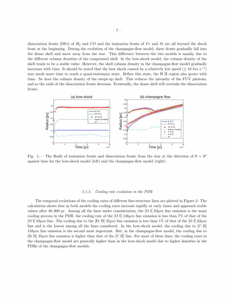
In Figure 1, the locations of various ionization fronts and dissociation fronts on the symmetry axis
are plotted as a function of time for both models. The figure shows that The distances between the star,
the ionization front and the dissociation front in the bow-shock model remain roughly constant while these
fronts move away from the star in the champagne-flow model. Moreover, in the champagne-flow model, the
– 7 –
dissociation fronts (DFs) of H2 and CO and the ionization fronts of Fe and Si are all beyond the shock
front at the beginning. During the evolution of the champagne-flow model, these fronts gradually fall into
the dense shell and move away from the star. This difference between the two models is mainly due to
the different column densities of the compressed shell. In the bow-shock model, the column density of the
shell tends to be a stable value. However, the shell column density in the champagne-flow model gradually
increases with time. It should be noted that the bow shock caused by a relatively low speed (≤ 10 km s−1)
star needs more time to reach a quasi-stationary state. Before this state, the H II region also grows with
time. So does the column density of the swept-up shell. This reduces the intensity of the FUV photons,
and so the radii of the dissociation fronts decrease. Eventually, the dense shell will overtake the dissociation
fronts.
0 2 4 6 8 10
x 104
0
0.05
0.1
0.15
0.2
0.25
0.3
Time [yr]
Rad
ius
[pc]
(a) bow shock
IF of HDF of H
2
DF of CORadius of bubbleSF
0 2 4 6 8 10
x 104
0
0.05
0.1
0.15
0.2
0.25
0.3
0.35
0.4
0.45
0.5
Time [yr]
Rad
ius
[pc]
(b) champagne flow
IF of HDF of H
2
DF of CORadius of bubbleIF of FeIF of SiSF
Fig. 1.— The Radii of ionization fronts and dissociation fronts from the star at the direction of θ = 0o
against time for the bow-shock model (left) and the champagne-flow model (right).
3.1.3. Cooling rate evolution in the PDR
The temporal evolutions of the cooling rates of different fine-structure lines are plotted in Figure 2. The
calculation shows that in both models the cooling rates increase rapidly at early times and approach stable
values after 40, 000 yr. Among all the lines under consideration, the [O I] 63µm line emission is the main
cooling process in the PDR. the cooling rate of the [O I] 146µm line emission is less than 7% of that of the
[O I] 63µm line. The cooling due to the [Fe II] 35µm line emission is less than 1% of that of the [O I] 63µm
line and is the lowest among all the lines considered. In the bow-shock model, the cooling due to [C II]
158µm line emission is the second most important. But, in the champagne-flow model, the cooling due to
[Si II] 35µm line emission is higher than that of the [C II] line. For most of these lines, the cooling rates in
the champagne-flow model are generally higher than in the bow-shock model due to higher densities in the
PDRs of the champagne-flow models.

– 8 –
0 2 4 6 8 10
x 104
31.5
32
32.5
33
33.5
34
34.5
35
35.5
36
36.5
Time [yr]
log(
Λ)
[erg
s−
1 ](a) bow shock
C II 158 µm
O I 63 µm
O I 146 µm
Si II 35 µm
Fe II 26 µm
Fe II 35 µm
0 2 4 6 8 10
x 104
31.5
32
32.5
33
33.5
34
34.5
35
35.5
36
36.5
Time [yr]
log(
Λ)
[erg
s−
1 ]
(b) champagne flow
C II 158 µm
O I 63 µm
O I 146 µm
Si II 35 µm
Fe II 26 µm
Fe II 35 µm
Fig. 2.— The variation of the cooling rate due to the fine-structure lines in PDR for the bow-shock model
(left) and the champagne-flow model (right).
3.2. Bow-shock models
We simulate two bow-shock models in the uniform medium. The parameters assumed in model A are
the same as those in the bow-shock model mentioned in 3.1. In model B, the 21.9 M⊙ star is replaced with
a 40.9 M⊙ star. For the new star, the ionizing and dissociating photon luminosities are 1048.78 s−1 and
1048.76 s−1, respectively. The effective temperature is 40, 000 K. The stellar wind mass-loss rate and the
terminal velocity are adopted to be M = 9.93×10⁻⁷ M⊙yr−1 and vw = 2720.1 km s−1, respectively. In both
models, the stellar velocity is v∗ = 15 km s−1. Again, these parameters are taken from Diaz-Miller et al.
(1998) and Dale et al. (2013). We carry out the simulation in the rest frame of the star in order to use the
same procedures as in the champagne-flow cases. The calculated velocities are then converted to the values
in the rest frame of the molecular cloud. In all models, the z-axis is parallel to the symmetry axis and the
positive direction is from the tail to the head of the cometary H II region. The position of the star is at
(r, z) = (0, 0).
We cease the simulations at 100, 000 yr. The density distributions of all materials, the H atoms, the
H+ ions and the warm H2 molecules in models A and B at the age of 100, 000 yr are presented in Figure 3,
together with the velocity fields. We compared the distributions at 100, 000 yr with those at age of 80, 000 yr,
which are not presented in the current work, and found that the appearance of the cometary H II region
does not changed significantly for more than twenty thousand years. So we conclude that the bow shock has
entered a quasi-stationary stage. In model A, a low-density and hot stellar-wind bubble (T > 106 K and
n < 5 cm−3) forms around the moving star. The photoionized region enveloped by a dense shell surrounds
the hot bubble. In this region, the densities are n ∼ 200− 20000 cm−3, and the temperatures are close to
T = 10000 K. A shell outside of the photoionized H II region is made of the compressed neutral gas with
density and temperature n ∼ 50000 cm−3 and T ∼ 400 K. The temperature in the neutral region outside
of the shell decreases gradually from ∼ 500 K near the IF to ∼ 50 K in the depth of the molecular cloud.
The top panels of Figure 3 show that a part of ionized gas in the tail is recombining. This is because the
ionizing photon flux decreases with distance from the star. The H2 dissociation front keeps a distance from
the dense shell ahead of the apex of H II region, but it falls into the dense shell at the sides because the
flux of dissociation photons reduces along the shell due to the increasing distance and the higher column

– 9 –
density of the shell at the sides. In model B, the structure of the H II region is similar to that in model A.
However, because of the presence of a more massive star in model B, the sizes of the photoionized region
and stellar-wind bubble are larger. And there is no indication of recombining gas in the tail because the
ionizing photon flux is still high enough to keep all material ionized there. The figure also shows that the
PDR in model B is not significantly bigger than that in model A. This is due to the longer distance between
the star and the shell and the higher density of the shell in model B.
Z [pc]
R [p
c]
(b)
log(
n) [c
m−
3 ]
−0.5 −0.4 −0.3 −0.2 −0.1 0 0.1 0.2 0.3
−0.4
−0.3
−0.2
−0.1
0
0.1
0.2
0.3
0.4
0.5
1.5
2.5
3.5
4.5
5.5
Z [pc]
R [p
c]
(c)
log(
n) [c
m−
3 ]
−0.6 −0.4 −0.2 0 0.2 0.4
−0.6
−0.4
−0.2
0
0.2
0.4
0.6
0.5
1.5
2.5
3.5
4.5
5.5
Z [pc]
R [p
c]
(d)
log(
n) [c
m−
3 ]−0.6 −0.4 −0.2 0 0.2 0.4
−0.6
−0.4
−0.2
0
0.2
0.4
0.6
0.5
1.5
2.5
3.5
4.5
5.5
Fig. 3.— The number density distributions of all materials, ionized hydrogen, hydrogen atoms and hydrogen
molecules at the rotational level of J = 4 in models A and B at the age of 100, 000 yr. The top panels and
the bottom panels are for models A and B, respectively. The left panels show the densities of all materials
(top half) and the H+ ions (bottom half). The right panels show those of H atoms (top half) and H2
molecules (bottom half). The arrows show the velocity field, and only velocities higher than 1 km s−1 are
presented, but the velocity field in the stellar-wind bubble is not shown.
3.2.1. Profiles and diagrams of the [Ne II] 12.81 line
The profiles of the [Ne II] 12.81 line for the inclinations of θ = 30o, 45o, and 60o are presented in
Figure 4. The differences between the profiles from model A and model B are not large. We also show

– 10 –
the properties of the [Ne II] line in Table 1. The computed profiles of the [Ne II] line are all negative-
skewed. The skewnesses of the line profiles in model A are −0.59, − 0.50, and − 0.33 for the inclinations
of θ = 30o, 45o, and 60o, respectively. And those in model B are −0.61, − 0.51, and − 0.34 for the three
inclination angles. It seems that the skewness of the [Ne II] line profiles in bow-shock models correlates
with the inclination but not the stellar mass. The flux weighted central velocities (FWCVs) of the [Ne
II] line profiles are 0.03, 0.02, 0.02 km s−1 in model A and 0.91, 0.74, 0.52 km s−1 in model B for
θ = 30o, 45o, and 60o, respectively. The larger EUV flux and the stronger stellar wind in model B result
in a larger proportion of the red-shifted ionized gas, therefore slightly more red-shifted FWCVs of the
line profiles. Because Gaussian fitting of the line profiles are the routine procedure in observations, we
provide the fitting results in the current work as well. In models A and B, the centers of the fitting curves
are all red-shifted (1.87, 1.35, and 0.73 km s−1 for θ = 30o, 45o, and 60o in model A, 2.51, 1.96, and
1.25 km s−1 in model B). Both the centers of the fitting curves and the FWCVs in the two bow-shock
models are much lower than the projected stellar velocities along the line of sight. This is because the
pressure gradient caused by the density gradient formed in the H II region leads to an acceleration generally
along the direction toward the tail. This acceleration causes the ionized gas to move slower than the star along
the symmetric axis. Although a component of acceleration also exists along the direction perpendicular to the
axis. Apparently, this perpendicular acceleration does not contribute significantly to the projected velocity
component along the line of sight. The details of this phenomenon has been discussed in Zhu & Zhu (2015).
The full width half maximum (FWHM) of the fitting curves in models A and B is 20.66, 18.13, 15.51 km s−1
and 18.33, 16.66, 14.82 km s−1, respectively. It is obvious that the FWHM decreases with increasing angle.
In Figure 4, the [Ne II] line profile becomes more Gaussian with the increasing inclination angle. The [Ne
II] line profiles from the slit (20 cells wide) along the symmetry axis of the projected 2D image for the three
inclinations in models A and B are also presented in Figure 4. The profiles from the slit are obviously more
red-shifted than the corresponding profiles from the whole H II region. This is because the influence of
the dense and red-shifted gases in the head of H II region is enforced, and the contribution to the profiles
from the low-density blue-shifted region is weakened when the line profiles are only computed from the
slit (Zhu & Zhu 2015). In addition, the profiles at the resolution of SOFIA/EXES instrument are shown in
Figure 4. Because the thermal broadening of Ne+ ions is comparable to the broadening at the slit resolution,
these ’realistic’ profiles are not very different from the ’ideal’ [Ne II] line profiles.
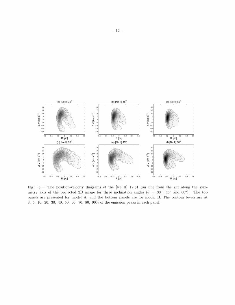
In Figure 5, the position-velocity diagrams of the [Ne II] line from the slit along the symmetry axis of
the projected 2D image in models A and B are shown for three inclination angles θ = 30o, 45o, and 60o. It
can be seen that the line emission distribution is made of two branches. These two branches are contributed
by the near and far sides of the shell like H II region. Because the density in the hot stellar-wind bubble is
extremely low compared with the density of the photoionized H II region, the contribution from the bubble
to the [Ne II] line luminosity is negligible. This causes the empty area between the two branches. In the
p-v diagrams of the [Ne II] line, the peaks are all red-shifted and gradually move towards 0 km s−1 with
increasing angles. The range of the velocity distribution of the line becomes narrower with the increasing
angle so that the emission peak becomes more concentrated. In model A, the density of the Ne+ ions is
the highest at the apex (n ∼ 10000 cm−3 and X(Ne+) = 0.84) and decreases to lower values in the tail
(n ∼ 300 cm−3 and X(Ne+) = 0.80). The emission from the apex is also higher than from the rest part of
the ionized region. As the inclination angle increases, the projection of the head region on the slit becomes
narrower. Hence, the bright areas are more concentrated in the p-v diagram for the inclinations of θ = 60o
than in the diagrams for lower inclination angles. In model B, the large size of the H II region leads to large
projected images. The separations between two branches in p-v diagrams of model B are larger than those
of model A. This is due to the larger cavity and opening angle of the H II region in model B.

– 11 –
−40 −30 −20 −10 0 10 20 30 400
0.2
0.4
0.6
0.8
1
∆ V [km/s]
Nor
mal
ised
Flu
x
(a) [Ne II] 30o
line profileGaussian fittingprofile from slitR=86,000
−40 −30 −20 −10 0 10 20 30 400
0.2
0.4
0.6
0.8
1
∆ V [km/s]
Nor
mal
ised
Flu
x
(b) [Ne II] 45o
line profileGaussian fittingprofile from slitR=86,000
−40 −30 −20 −10 0 10 20 30 400
0.2
0.4
0.6
0.8
1
∆ V [km/s]
Nor
mal
ised
Flu
x
(c) [Ne II] 60o
line profileGaussian fittingprofile from slitR=86,000
−40 −30 −20 −10 0 10 20 30 400
0.2
0.4
0.6
0.8
1
∆ V [km/s]
Nor
mal
ised
Flu
x
(d) [Ne II] 30o
line profileGaussian fittingprofile from slitR=86,000
−40 −30 −20 −10 0 10 20 30 400
0.2
0.4
0.6
0.8
1
∆ V [km/s]
Nor
mal
ised
Flu
x
(e) [Ne II] 45o
line profileGaussian fittingprofile from slitR=86,000
−40 −30 −20 −10 0 10 20 30 400
0.2
0.4
0.6
0.8
1
∆ V [km/s]
Nor
mal
ised
Flu
x
(f) [Ne II] 60o
line profileGaussian fittingprofile from slitR=86,000
Fig. 4.— Profiles of the [Ne II] line (solid lines), the Gaussian fitting to the profiles (dashed lines) and the
profiles at the resolution of R = 86, 000 (dot-dashed lines) at three inclination angles (θ = 30o, 45o and 60o).
The [Ne II] line profiles from the slit along the symmetry axis of the projected 2D image are also plotted
(dotted lines). The top panels are plotted for model A, and the bottom panels are for model B
– 12 –
∆ V
[km
s−
1 ]
R [pc]
(a) [Ne II] 30o
−0.6 −0.4 −0.2 0 0.2 0.4 0.6
−20
−15
−10
−5
0
5
10
15
20
∆ V
[km
s−
1 ]
R [pc]
(b) [Ne II] 45o
−0.6 −0.4 −0.2 0 0.2 0.4 0.6
−20
−15
−10
−5
0
5
10
15
20
∆ V
[km
s−
1 ]
R [pc]
(c) [Ne II] 60o
−0.6 −0.4 −0.2 0 0.2 0.4 0.6
−20
−15
−10
−5
0
5
10
15
20
∆ V
[km
s−
1 ]
R [pc]
(d) [Ne II] 30o
−0.6 −0.4 −0.2 0 0.2 0.4 0.6
−20
−15
−10
−5
0
5
10
15
20
∆ V
[km
s−
1 ]
R [pc]
(e) [Ne II] 45o
−0.6 −0.4 −0.2 0 0.2 0.4 0.6
−20
−15
−10
−5
0
5
10
15
20∆
V [k
m s
−1 ]
R [pc]
(f) [Ne II] 60o
−0.6 −0.4 −0.2 0 0.2 0.4 0.6
−20
−15
−10
−5
0
5
10
15
20
Fig. 5.— The position-velocity diagrams of the [Ne II] 12.81 µm line from the slit along the sym-
metry axis of the projected 2D image for three inclination angles (θ = 30o, 45o and 60o). The top
panels are presented for model A, and the bottom panels are for model B. The contour levels are at
3, 5, 10, 20, 30, 40, 50, 60, 70, 80, 90% of the emission peaks in each panel.

– 13 –
3.2.2. Profiles and diagrams of the H2 S(2) line
The profiles of the H2 S(2) line for three inclinations of θ = 30o, 45o and 60o are shown in Figure 6. The
properties of this line are shown in Table 1. It is different from the [Ne II] line in that the profiles of the H2
line in the two bow-shock models are positive-skewed. The skewnesses of the H2 S(2) line profiles in model
A are 0.72, 0.86, 0.75 for θ = 30o, 45o, 60o, respectively. And those in model B are 0.22, 0.29, and 0.26 for
the three inclination angles. It is obvious that no general trend of skewness as in [Ne II] line case exists in
H2 S(2) line. At the same time, profiles of the H2 S(2) line are generally far from a Gaussian distribution.
In particular, the line profiles for the inclination of 45o and 60o in model B are double-peaked. Therefore,
the skewness of the H2 S(2) line profile is not a good indicator of the inclination angle. The FWCVs of the
H2 S(2) line profiles are 1.94, 1.58, and 1.12 km s−1 for the inclination angles θ = 30o, 45o, and 60o in
model A, respectively. Those in model B are 4.81, 3.93, and 2.78 km s−1 for the corresponding inclinations.
And the centers of the Gaussian fitting for the three inclinations are 1.14, 0.38, 0.09 km s−1 in model A and
4.63, 3.55, 2.36 km s−1 in model B. All these values of the H2 line are much less than the stellar velocities.
However, a decreasing trend with increasing inclination is still observed. The FWHMs of the fitting curves
in models A and B are 5.16, 3.82, 4.25 km s−1 and 8.27, 9.54, 10.45 km s−1 for the inclinations of 30o, 45o
and 60o, separately. The FWCVs and the centers of the fitting curves in the H2 S(2) line in model B
are higher than those in model A, and the FWHMs in model B are also larger than in model A. This is
because the proportion of the warm molecular gas compressed in the shell is higher in model B. It is worth
noting that the FWHM of the H2 S(2) line does not decrease with increasing angle. This is different from
the [Ne II] line case. The FWHM in model B even increases with the inclination angles. The line profiles
of the H2 line from the slit along the symmetry axis of the projected 2D image are shown in Figure 6 as
well. We find that the double peak is more apparent in the profiles from the slit than in those from the
whole neutral region. This is because the contribution from the gas above and below the plane of the slit
is reduced. This part of gas has velocities distributed in between two the extreme velocities represented by
the two peaks. The computed H2 line profiles are convolved with the thermal and instrumental broadening
kernel to predict the line profiles of simulated observations. The results show that the broadening does not
significantly degrade our ability to extract the necessary kinematical information, since the line center can
still be estimated reliably from observations.
In Figure 7, the position-velocity diagrams of the H2 S(2) line from the slit along the symmetry axis of
the projected 2D image in models A and B are presented for the inclinations of θ = 30o, 45o, and 60o. As
already demonstrated in previous figures, a large part of H2 line emitting warm molecular gas does not exist
close to the apex of the shell but exists in the shell at the sides and the undisturbed region beyond the shock
front. So the H2 rotational line emission peaks are not obviously red-shifted. These diagrams also show the
difference in the projected velocities of the warm molecular gas between the two sides of the cometary H II
region. The projected velocity of the molecular gas in the near side of the shell and the region outside of
the shell is close to zero, and that from the gas at the farther side of the shell is higher than 5 km s−1. In
addition, the molecular gas in the apex of the dense shell in model B has a high velocity ∆v ≥ 10 km s−1,
similar to the stellar velocity. But in model A, the apex of the dense shell is almost fully dissociated. There
is no such high velocity component shown in the p-v diagrams for model A.

– 14 –
−15 −10 −5 0 5 10 150
0.2
0.4
0.6
0.8
1
∆ V [km/s]
Nor
mal
ised
Flu
x
(a) H2 4−2 30o
line profileGaussian fittingprofile from slitR=86,000
−15 −10 −5 0 5 10 150
0.2
0.4
0.6
0.8
1
∆ V [km/s]
Nor
mal
ised
Flu
x
(b) H2 4−2 45o
line profileGaussian fittingprofile from slitR=86,000
−15 −10 −5 0 5 10 150
0.2
0.4
0.6
0.8
1
∆ V [km/s]
Nor
mal
ised
Flu
x
(c) H2 4−2 60o
line profileGaussian fittingprofile from slitR=86,000
−15 −10 −5 0 5 10 15 200
0.2
0.4
0.6
0.8
1
∆ V [km/s]
Nor
mal
ised
Flu
x
(d) H2 4−2 30o
line profileGaussian fittingprofile from slitR=86,000
−15 −10 −5 0 5 10 15 200
0.2
0.4
0.6
0.8
1
∆ V [km/s]
Nor
mal
ised
Flu
x(e) H
2 4−2 45o
line profileGaussian fittingprofile from slitR=86,000
−15 −10 −5 0 5 10 15 200
0.2
0.4
0.6
0.8
1
∆ V [km/s]
Nor
mal
ised
Flu
x
(f) H2 4−2 60o
line profileGaussian fittingprofile from slitR=86,000
Fig. 6.— Profiles of the H2 S(2) line (solid lines), the Gaussian fitting to the profiles (dashed lines) and the
profiles at the resolution of R = 86, 000 (dot-dashed lines) at three inclination angles (θ = 30o, 45o and 60o).
The H2 S(2) line profiles from the slit along the symmetry axis of the projected 2D image are also presented
(dotted lines). The top panels are plotted for model A, and the bottom panels are shown for model B.
Model A Bow shock 21.9 M⊙
Line Inclination FWCV Skewness Center of line FWHM
(km s−1) (km s−1) (km s−1)
[Ne II] 12.81µm 30o 0.03 -0.59 1.87 20.69
45o 0.02 -0.50 1.35 18.34
60o 0.02 -0.33 0.73 15.58
H2 4− 2 30o 1.94 0.72 1.14 5.16
45o 1.58 0.86 0.38 3.82
60o 1.12 0.75 0.09 4.25
Model B Bow shock 40.9 M⊙
Line Inclination FWCV Skewness Center of line FWHM
(km s−1) (km s−1) (km s−1)
[Ne II] 12.81µm 30o 0.91 -0.61 2.51 18.33
45o 0.74 -0.51 1.96 16.66
60o 0.52 -0.34 1.25 14.82
H2 4− 2 30o 4.81 0.22 4.63 8.27
45o 3.93 0.29 3.55 9.54
60o 2.78 0.26 2.36 10.45
Table 1: Flux weighted central velocities (FWCV), skewness, and the center and FWHMs of Gaussian fitting
of the lines for different angles in models A and B

– 15 –
∆ V
[km
s−
1 ]
R [pc]
(a) H2 4−2 30o
−0.6 −0.4 −0.2 0 0.2 0.4 0.6
−20
−15
−10
−5
0
5
10
15
20
∆ V
[km
s−
1 ]
R [pc]
(b) H2 4−2 45o
−0.6 −0.4 −0.2 0 0.2 0.4 0.6
−20
−15
−10
−5
0
5
10
15
20
∆ V
[km
s−
1 ]
R [pc]
(c) H2 4−2 60o
−0.6 −0.4 −0.2 0 0.2 0.4 0.6
−20
−15
−10
−5
0
5
10
15
20
∆ V
[km
s−
1 ]
R [pc]
(d) H2 4−2 30o
−0.6 −0.4 −0.2 0 0.2 0.4 0.6
−20
−15
−10
−5
0
5
10
15
20
∆ V
[km
s−
1 ]
R [pc]
(e) H2 4−2 45o
−0.6 −0.4 −0.2 0 0.2 0.4 0.6
−20
−15
−10
−5
0
5
10
15
20∆
V [k
m s
−1 ]
R [pc]
(f) H2 4−2 60o
−0.6 −0.4 −0.2 0 0.2 0.4 0.6
−20
−15
−10
−5
0
5
10
15
20
Fig. 7.— The position-velocity diagrams of the H2 4 − 2 rotational line from the slit along the symme-
try axis of the projected 2D image for three inclination angles (θ = 30o, 45o and 60o). The top pan-
els and the bottom panels are shown for model A and model B, respectively. The contour levels are at
3, 5, 10, 20, 30, 40, 50, 60, 70, 80, 90% of the emission peaks in each panel.

– 16 –
3.3. Champagne-Flow Models
In models C and D, the evolutions of a champagne flow including a stellar wind are simulated. The
parameters in model C are the same as those in the champagne-flow model mentioned in 3.1. A 40.9 M⊙
massive star is assumed in model D, and other parameters in model D are the same as in model C. The
simulations of models C and D are also stopped at 100, 000 yr. At that time, the champagne flows have
cleared the low-density material from the grid.
The density distributions in models C and D are presented in Figure 8. The size of the H II region in
models C and D is much larger than that in models A and B. Due to the high density in the molecular cloud
and the large distance from the shell to the star, the ionization front and the dissociation fronts of H2 and
CO are close to each other and all fall into the shell at a certain age.
Z [pc]
R [p
c]
(b)
log(
n) [c
m−
3 ]
−1.5 −1 −0.5 0 0.5 1
−1
−0.5
0
0.5
10.5
1.5
2.5
3.5
4.5
5.5
Z [pc]
R [p
c]
(d)
log(
n) [c
m−
3 ]
−1.5 −1 −0.5 0 0.5 1
−1
−0.5
0
0.5
10.5
1.5
2.5
3.5
4.5
5.5
Fig. 8.— The density distributions of all materials, ionized hydrogen, hydrogen atoms and hydrogen
molecules at the rotational level of J = 4 in models C and D at the age of 100, 000 yr. The top panels
and the bottom panels are presented for models C and D, respectively. The left panels show the densities of
all materials (top half) and the H+ ions (bottom half). The right panels show those of H atoms (top half)
and H2 molecules (bottom half). The arrows in the left panels represent velocities of v ≥ 1 km s−1, but the
velocity field in stellar-wind bubbles are not shown.
– 17 –
3.3.1. Profiles and diagrams of the [Ne II] 12.81 line
A part of the ionized region in model C and model D is outside of the grid and not shown in Figure 8.
However, since more than 80 percent of the [Ne II] line emission in model C is emitted by the region with
z ≥ −0.5 pc, the line emission from the region outside of the grid in models C and D should be small. The
profiles of the [Ne II] line and the Gaussian fitting to the profiles for three inclinations in models C and D
are presented in Figure 9. The properties of the [Ne II] line profiles are listed in Table 2. In model C, the
FWCVs of the [Ne II] line profiles are −7.54, − 6.16, and − 4.36 km s−1 for three inclinations of 30o, 45o,
and 60o respectively, and the centers of the Gaussians are −6.16, − 4.99, and − 3.49 km s−1. In model
D, the FWCVs of the [Ne II] line profiles are −5.42, − 4.42, and − 3.13 km s−1 for the three inclinations,
and the centers of the fitting curves are −4.23, − 3.41, and − 2.36 km s−1. These values are all obviously
blue-shifted. The FWHMs of the Gaussian fitting are 14.91, 12.91, and 11.00 km s−1 in model C and
13.43, 11.75, 10.40 km s−1 in model D. These FWHMs are apparently lower than those in the bow-shock
models. The velocity of the ionized gas in both the bow-shock models and the champagne-flow models
approaches vz ∼ −20 km s−1. In the head of the photoionized region, the axial velocities of the ionized gas
in the bow-shock models can reach the stellar velocity. But, it is at most 1 km s−1 in the champagne-flow
models. As the result, the FWHMs of the [Ne II] line in the bow-shock models are larger than those in the
champagne-flow models. The [Ne II] line profiles in models C and D are also negative skewed like those in
models A and B. The skewnesses in models C and D are −0.68, − 0.70, − 0.67 and −0.76, − 0.81, − 0.79
for the inclinations of θ = 30o, 45o, 60o, respectively. The skewnesses for the inclinations of θ = 70o, 80o are
also calculated but not listed in Table 2. These skewnesses are −0.58, − 0.35 in model C and −0.57, − 0.34
in model D for θ = 70o, 80o, respectively. The trend that the skewness of the [Ne II] line profile increases
from more negative values toward zero also exists in the champagne-flow models, but it is not obvious when
the inclination angle is smaller than 45o. This may be due to large opening angles of the cometary H II
region in the champagne-flow models. The [Ne II] line profiles from the slit along the symmetry axis of the
projected 2D image in models C and D are also shown in Figure 9. The profiles are more red-shifted than
those from the whole region as in models A and B. However, In the champagne-flow models, the profiles
from the slit are more similar to those of the entire region.
In Figure 10, the position-velocity diagrams of the [Ne II] line from the slit along the symmetry axis
of the projected 2D image for three inclination angles in the two champagne-flow models are presented. In
the diagrams, the main part of the flux is located at the position of ∆v < 0 km s−1. In models C and D,
only the ionized gas close to the ionization front may have a red-shifted velocity component, and the ionized
materials in the rest part of the H II region flow towards the tail. As in the bow-shock models, the emission
becomes more concentrated with increasing inclination in models C and D. There are also two branches in
every diagram in Figure 10. In these diagrams, the velocity range of the left branch (R < 0) is wider than
that of the other branch (R > 0). This is because the gas contributing emission to the left branch is from the
near side of the shell. The angle between this side of the shell and the line of sight is smaller. The velocity
projection onto the line of sight is more efficient than that of the gas moving approximately perpendicular
to the line of sight, which is the case for the gas in the farther side of the shell.
3.3.2. Profiles and diagrams of the H2 S(2) line
The profiles of the H2 S(2) line are plotted in Figure 11, and their line properties are listed in Table
2. The FWCVs of the H2 line and the centers of the Gaussian fitting curves are 0.99, 0.81, 0.57 km s−1

– 18 –
−40 −30 −20 −10 0 10 20 30 400
0.2
0.4
0.6
0.8
1
∆ V [km/s]
Nor
mal
ised
Flu
x
(a) [Ne II] 30o
line profileGaussian fittingprofile from slitR=86,000
−40 −30 −20 −10 0 10 20 30 400
0.2
0.4
0.6
0.8
1
∆ V [km/s]
Nor
mal
ised
Flu
x
(b) [Ne II] 45o
line profileGaussian fittingprofile fron slitR=86,000
−40 −30 −20 −10 0 10 20 30 400
0.2
0.4
0.6
0.8
1
∆ V [km/s]
Nor
mal
ised
Flu
x
(c) [Ne II] 60o
line profileGaussian fittingprofile from slitR=86,000
−40 −30 −20 −10 0 10 20 30 400
0.2
0.4
0.6
0.8
1
∆ V [km/s]
Nor
mal
ised
Flu
x
(d) [Ne II] 30o
line profileGaussian fittingprofile from slitR=86,000
−40 −30 −20 −10 0 10 20 30 400
0.2
0.4
0.6
0.8
1
∆ V [km/s]
Nor
mal
ised
Flu
x
(e) [Ne II] 45o
line profileGaussian fittingprofile from slitR=86,000
−40 −30 −20 −10 0 10 20 30 400
0.2
0.4
0.6
0.8
1
∆ V [km/s]
Nor
mal
ised
Flu
x
(f) [Ne II] 60o
line profileGaussian fittingprofile from slitR=86,000
Fig. 9.— Profiles of the [Ne II] line (solid lines), the Gaussian fitting to the profiles (dashed lines) and the
profiles at the resolution of R = 86, 000 (dot-dashed lines) at three inclination angles (θ = 30o, 45o and 60o).
The [Ne II] line profiles from the slit along the symmetry axis of the projected 2D image are also plotted
(dotted lines). The top panels are plotted for model C, and the bottom panels are for model D.

– 19 –
∆ V
[km
s−
1 ]
R [pc]
(a) [Ne II] 30o
−1 −0.5 0 0.5 1
−20
−15
−10
−5
0
5
10
15
20
∆ V
[km
s−
1 ]
R [pc]
(b) [Ne II] 45o
−1 −0.5 0 0.5 1
−20
−15
−10
−5
0
5
10
15
20
∆ V
[km
s−
1 ]
R [pc]
(c) [Ne II] 60o
−1 −0.5 0 0.5 1
−20
−15
−10
−5
0
5
10
15
20
∆ V
[km
s−
1 ]
R [pc]
(d) [Ne II] 30o
−1 −0.5 0 0.5 1
−20
−15
−10
−5
0
5
10
15
20
∆ V
[km
s−
1 ]
R [pc]
(e) [Ne II] 45o
−1 −0.5 0 0.5 1
−20
−15
−10
−5
0
5
10
15
20∆
V [k
m s
−1 ]
R [pc]
(f) [Ne II] 60o
−1 −0.5 0 0.5 1
−20
−15
−10
−5
0
5
10
15
20
Fig. 10.— The position-velocity diagrams of the [Ne II] 12.81 µm line from the slit along the sym-
metry axis of the projected 2D image for three inclination angles (θ = 30o, 45o and 60o). The top
panels are presented for model C, and the bottom panels are for model D. The contour levels are at
3, 5, 10, 20, 30, 40, 50, 60, 70, 80, 90% of the emission peaks in each panel.

– 20 –
and 1.04, 0.87, 0.62 km s−1 for inclination angles of 30o, 45o and 60o in model C, respectively, and those
in model D are 1.73, 1.41, 1.00 km s−1 and 1.65, 1.33, 0.94 km s−1. The FWCV and the line centers are
close to each other for the corresponding inclinations because the line profiles are very close to Gaussian.
All values in model D are a little higher than the corresponding ones in model C. This is because the higher-
mass star with larger ionization luminosity and stronger stellar wind in model D leads to a faster moving
ionization front. The FWHMs of the fitted Gaussian in models C and D are 4.00, 4.76, 5.40 km s−1 and
4.03, 4.79, 5.45 km s−1 for inclination angles of 30o, 45o, 60o, respectively. It is apparent that the FWHM
increases with rising inclination angle. It is not easy to distinguish models C and D from model A with
the same stellar parameters by only using the FWCVs, FWHMs and the centers of the fitting curves of the
H2 S(2) line. Particularly, the inclination angle causes more ambiguities. The FWCVs of the H2 S(2) line
in model B are obviously higher than those in the other models. Although the profiles of the H2 line are
closer to a Gaussian shape in the champagne-flow models, the difference of the line profiles is not significant
enough. In addition, the skewnesses of the H2 S(2) line profiles in models C and D are 0.01, − 0.03, − 0.03
and 0.26, 0.20, 0.13 for the inclinations of 30o, 45o, and 60o, respectively. The skewnesses of the H2 line
in champagne flows are generally lower than in bow shocks. The H2 line profiles from the slit along the
symmetry axis of the projected 2D image for the three inclinations in models C and D are hard to distinguish
from the ones for the whole regions.
−15 −10 −5 0 5 10 150
0.2
0.4
0.6
0.8
1
∆ V [km/s]
Nor
mal
ised
Flu
x
(a) H2 4−2 30o
line profileGuassian fittingprofile from slitR=86,000
−15 −10 −5 0 5 10 150
0.2
0.4
0.6
0.8
1
∆ V [km/s]
Nor
mal
ised
Flu
x
(b) H2 4−2 45o
line profileGaussian fittingprofile from slitR=86,000
−15 −10 −5 0 5 10 150
0.2
0.4
0.6
0.8
1
∆ V [km/s]
Nor
mal
ised
Flu
x
(c) H2 4−2 60o
line profileGaussian fittingprofile from slitR=86,000
−15 −10 −5 0 5 10 150
0.2
0.4
0.6
0.8
1
∆ V [km/s]
Nor
mal
ised
Flu
x
(d) H2 4−2 30o
line profileGaussian fittingprofile from slitR=86,000
−15 −10 −5 0 5 10 150
0.2
0.4
0.6
0.8
1
∆ V [km/s]
Nor
mal
ised
Flu
x
(e) H2 4−2 45o
line profileGaussian fittingprofile from slitR=86,000
−15 −10 −5 0 5 10 150
0.2
0.4
0.6
0.8
1
∆ V [km/s]
Nor
mal
ised
Flu
x
(f) H2 4−2 60o
line profileGaussian fittingprofile from slitR=86,000
Fig. 11.— Profiles of the H2 S(2) line (solid lines), the Gaussian fitting to the profiles (dashed lines) and the
profiles at the resolution of R = 86, 000 (dot-dashed lines) at three inclination angles (θ = 30o, 45o and 60o).
The H2 S(2) line profiles from the slit along the symmetry axis of the projected 2D image are also presented
(dotted lines). The top panels are plotted for model C, and the bottom panels are shown for model D.
The position-velocity diagrams of the H2 S(2) line from the slit along the symmetry axis of the projected
2D image for the inclination angles of 30o, 45o, 60o in models C and D (Figure 12) are obviously different
from those in bow-shock models. The axial components of the velocity of the molecular hydrogen in models
C and D are not high. There is apparently no gas emission above 5 km s−1 in the diagrams. The H2 line

– 21 –
emission is always close to the red-shifted side of the [Ne II] line emission at the same values of R. This is
because the H2 dissociation front falls into the dense shell almost in every direction in models C and D so
that the H2 line emission is all from the dense shell in the champagne-flow models and the distribution of
the H2 line emission is continuous. Both the [Ne II] line emission and the H2 line emission come from the
dense shell behind the shock front. Their dynamics is mainly due to the expansion of the H II region and
the dense shell. The projected velocities of the neutral gas in the shell are typically more red-shifted than
those of the nearby ionized gas. However, in the bow-shock models, part of the H2 line emission comes from
the region beyond the shock front. If the stellar velocity is not very high (v∗ ≤ 10 km s−1), the DF of H2
will also fall into the dense shell, and the H2 line emission from the molecular gas close to the apex of the
shell will reflect in the p-v diagrams. On the other hand, the number of H2 line photons emitted from the
region beyond the shock front is very small and can be neglected.
∆ V
[km
s−
1 ]
R [pc]
(a) H2 4−2 30o
−1 −0.5 0 0.5 1
−20
−15
−10
−5
0
5
10
15
20
∆ V
[km
s−
1 ]
R [pc]
(b) H2 4−2 45o
−1 −0.5 0 0.5 1
−20
−15
−10
−5
0
5
10
15
20
∆ V
[km
s−
1 ]
R [pc]
(c) H2 4−2 60o
−1 −0.5 0 0.5 1
−20
−15
−10
−5
0
5
10
15
20
∆ V
[km
s−
1 ]
R [pc]
(d) H2 4−2 30o
−1 −0.5 0 0.5 1
−20
−15
−10
−5
0
5
10
15
20
∆ V
[km
s−
1 ]
R [pc]
(e) H2 4−2 45o
−1 −0.5 0 0.5 1
−20
−15
−10
−5
0
5
10
15
20∆
V [k
m s
−1 ]
R [pc]
(f) H2 4−2 60o
−1 −0.5 0 0.5 1
−20
−15
−10
−5
0
5
10
15
20
Fig. 12.— The position-velocity diagrams of the H2 4-2 rotational transition line from the slit along the
symmetry axis of the projected 2D image for three inclination angles (θ = 30o, 45o and 60o). The top
panels are presented for model C, and the bottom ones are shown for model D. The contour levels are at
3, 5, 10, 20, 30, 40, 50, 60, 70, 80, 90% of the emission peaks in each panel.
3.4. Comparison with observations
Two cometary H II regions in the DR 21 region were observed by Cyganowski et al. (2003) to investigate
whether the H II regions are consistent with bow-shock models or champagne-flow models. The northern H
II region can be explained by a champagne-flow model. And the observations of the southern H II region
suggest a hybrid model including a stellar motion and a density gradient. Immer et al. (2014) presented deep
Very Large Array H66α observations of the southern cometary H II regions in DR 21. The line profiles of
H66α line from different positions in the H II regions are shown separately. The analysis of the observations
shows that the line profiles mostly show two velocity components. The ionized gas near the cometary head is

– 22 –
Model C Champagne Flow 21.9 M⊙
Line Inclination FWCV Skewness Center of line FWHM
(km s−1) (km s−1) (km s−1)
[Ne II] 12.81µm 30o -7.54 -0.68 -6.16 14.91
45o -6.16 -0.70 -4.99 12.91
60o -4.36 -0.67 -3.49 11.00
H2 4− 2 30o 0.99 0.01 1.04 4.00
45o 0.81 -0.03 0.87 4.76
60o 0.57 -0.03 0.62 5.40
Model D Champagne Flow 40.9 M⊙
Line Inclination FWCV Skewness Center of line FWHM
(km s−1) (km s−1) (km s−1)
[Ne II] 12.81µm 30o -5.42 -0.76 -4.23 13.43
45o -4.42 -0.81 -3.41 11.75
60o -3.13 -0.79 -2.36 10.40
H2 4− 2 30o 1.73 0.26 1.65 4.03
45o 1.41 0.20 1.33 4.79
60o 1.00 0.13 0.94 5.45
Table 2: Flux weighted central velocities (FWCV), skewness, and the center and FWHMs of Gaussian fitting
of the lines for different angles in models C and D
mainly blue-shifted (towards the cloud in the observations), and this is consistent with the results of our bow-
shock models. The velocity of the ionized gas becomes increasingly red-shifted from the head to the cometary
tail, and the ionized gas at the tail has a highly red-shifted velocity (∼ 30 km s−1) relative to the molecular
gas. Our champagne-flow models also show such kinematic features. Since, in the bow-shock models, the
ionized gas velocity at the tail can not reach such a high value, and the ionized gas near the cometary head
mainly flows downstream in our champagne-flow models, we agree that these features suggest the combined
effects of a stellar wind, stellar motion (as in bow-shock models) and an ambient density gradient (as in
champagne-flow models).
4. Conclusions
In this paper, we simulate the evolution of the cometary H II region with the PDR in bow-shock
models and champagne-flow models. The line profiles of the [Ne II] 12.81µm line and the H2 S(2) line are
presented, and the properties of these lines are studied. In the champagne-flow models, the ionized gas flows
downstream into the low-density region due to the pressure gradient caused by the original density gradient,
and the neutral gas in the dense shell enveloping the H II region moves slowly with the expansion of the
ionized region. In the bow-shock models, the ionized gas in the head of the cometary H II region originally
goes towards the molecular cloud with the moving star. But the ionized gas is gradually accelerated at the
opposite direction because of the density gradient formed in the ionized region, and eventually flows toward
the tail. The neutral dense shell moves in the direction of the stellar motion in bow-shock models. By
using the [Ne II] 12.81 µm line, it is possible to distinguish a high stellar velocity bow-shock model from
the champagne-flow models. If the center of the [Ne II] line profile from the head of the H II region has
a doppler shift that indicates an ionized gas motion toward the molecular cloud, the cometary H II region
should be caused by a bow shock. However, because the ionized gas is accelerated toward the tail, the line
profiles from a low speed star bow shock might be confused with those from a champagne flow. In this case,
it is possible to use the emission lines from the dense shell as additional criteria to discriminate between the

– 23 –
bow-shock and champagne-flow scenarios. This is because the neutral gas in the shell is not influenced by
the density gradient in the H II region. If the center of the H2 S(2) line profile from the molecular gas near
the cometary head has a doppler shift larger than 3 km s−1, it is likely a bow shock is present because such
a high speed of the molecular gas can not be reached only by the expansion of the ionized gas unless the H
II region is at very early times. The details of our models are summarized as follows:
1. In both the bow-shock and the champagne-flow models, the [Ne II] 12.81µm line profiles are negative-
skewed. The skewness of the [Ne II] line profiles increases from more negative values with the increasing
inclination. However, in the champagne-flow models, because of the large opening angle, this trend is not
obvious when the inclination is lower than 45o. The centers of the [Ne II] line profiles in the champagne-flow
models are obviously blue-shifted (FWCV < −3 km s−1). In the bow-shock models, because of the pressure
gradient in ionized regions mentioned above, the centers of the [Ne II] line could be blue-shifted when the
stellar velocity is v∗ < 15km s−1. If the stellar velocity is high, the centers of the [Ne II] line are red-shifted.
The FWHM of the Gaussian fitting of the [Ne II] line decreases with the increasing inclination in both the
bow-shock models and the champagne-flow models.
2. For the H2 S(2) line, we predict that the line centers are red-shifted in the bow-shock models when
the stellar velocity is high. But the center of the H2 line is always less than 5 km s−1. This is because
the apex of the dense shell is fully dissociated by the FUV photons if the stellar velocity is higher than
10 km s−1, and the emission is mostly from the sides of the dense shell and the undisturbed region where
the gas has less red-shifted velocity. Because of the discontinuity of the velocity field of the molecular gas in
shell, the H2 S(2) line profiles in the bow-shock models are far from Gaussian and often double-peaked. In
the champagne-flow models, the line profiles are very close to the Gaussian shape. And the centers of the
lines are lower than 2 km s−1 and limited by the expansion of the H II region.
3. The position-velocity diagrams of the [Ne II] line from the slit along the symmetry axis of the
projected 2D image show that the line tends to be blue-shifted in the champagne-flow models. In the bow-
shock models with stellar velocity v∗ = 15 km s−1, the emission peaks of the [Ne II] line are all red-shifted.
Comparing the p-v diagrams of the [Ne II] line and the H2 S(2) line, we find that the dynamics of the ionized
gas is influenced by pressure gradients in the ionized region for both the champagne-flow models and the
bow-shock models, but the H2 line emission is mainly affected by the moving shell or the expansion of the
ionized region. So the correlation between the kinematics of the ionized gas and that of the warm molecular
gas is low.
4. In the bow-shock model, the IF and the DFs are at roughly constant distances from the star after
a certain age. In the champagne-flow model, the distances from the star of the IF and DFs increase with
time. The DFs gradually fall into the dense shell along the evolution of the champagne flows.
Acknowledgements: The work is partially supported by National Basic Research Program of China (973
program) No. 2012CB821805 and the Strategic Priority Research Program ” The Emergence of Cosmological
Structures” of the Chinese Academy of Sciences. Grant No. XDB09000000. The authors are also grateful to
the supports by Doctoral Fund of Ministry of Education of China No. 20113402120018 and Natural Science
Foundation of Anhui Province of China No. 1408085MA13. F.-Y. Zhu thanks Dr. X.-L. Deng for generous
financial aids during the visit to Beijing Computational Science Research Center and suggestions on the
hydrodynamical computation methods, and also thanks Dr. J.-X. Wang for financial supports.

– 24 –
5. Appendix
5.1. Expansion of an H II region in a uniform medium
Two test cases are shown in Appendix to assess the reliability of our models. In the first test case,
we simulated the expansion of the H II region in a uniform medium of density n = 10000 cm−3 and initial
temperature T = 10 K. The effective temperature of the star is assumed to be 40, 000 K. The photo
luminosities of the ionizing radiation and dissociating radiation of the star are 1048.78 s−1 and 1048.76 s−1,
respectively. Stellar winds are not included. The grid has 250×500 uniform cells of size 0.005 pc. We ceased
the evolution at 100, 000 yr, and compared the results of this case with the analytical solution in Spitzer
(1978) and the numerical results of the expansion of the H II region and the PDR in Hosokawa & Inutsuka
(2006).
In Figure 13, the radial expansion of the numerical solution and the analytical solution of the spherical
H II region are compared. The analytical solution is given by Spitzer (1978) as follows,
RIF = R0(1 +7
4
cIIt
R0
)4/7 , (11)
where RIF is the radius of the ionization front. R0 is the radius of the theoretical initial Stomgren sphere.
cII is the sound speed of the ionized gas, and t is time. The percentage difference between the numerical
solution and the analytical solution is also shown in Figure 13. An approximate formula derived from the
equation of motion of the shell is provided by Hosokawa & Inutsuka (2006) as follows,
RIF = R0(1 +7
4
√
4
3
cIIt
R0
)4/7 . (12)
This formula and the percentage difference between it and the result of the test case are also plotted
in Figure 13. The numerical result is closer to the solution of Spitzer expansion at early times, and become
closer to the formula provided by Hosokawa & Inutsuka (2006) at late times. The percentage differences are
always lower than 10%.
The radial density and temperature distributions from the expansion of the spherical H II region in
the first test case are plotted in Figure 14. These results are compared with the results in Fig. 3 from
Hosokawa & Inutsuka (2006). Because of the same initial conditions, the results in our model are approxi-
mately consistent with those in Hosokawa & Inutsuka (2006). The temperature of ionized gas both in two
models is T ≈ 10000K, and the radial temperature distribution in PDR is similar. The density distributions
in the ionized region and PDR are also alike. But, since the resolution in the 1D model (Hosokawa & Inutsuka
2006) is higher than that in our 2D model, the results around the neutral dense shell in two models dif-
fer slightly. In Hosokawa & Inutsuka (2006), the temperature increases slightly near the H II region edge.
However, this phenomenon does not appear in our result because the effect of spectral hardening is not
considered. According to our calculations, this distinction will not lead to a significant difference.
5.2. Evolution of an H II region with a moving star
A second test case, comparing a simulation of a bow shock with the models in Mackey et al. (2015) is
also studied. In this case, the uniform density of the neutral medium is assumed to be n = 3000 cm−3,

– 25 –
0 2 4 6 8 10
x 104
0
0.1
0.2
0.3
0.4
0.5
0.6
0.7
0.8
0.9
1
Time [yr]
Rad
ius
[pc]
numerical resultSpitzer 1978Hosokawa 2006
0 2 4 6 8 10
x 104
0
2
4
6
8
10
12
14
16
18
20
Time [yr]
Diff
eren
ces
[%]
percentage difference from Spitzer 1978percentage difference from Hosokawa 2006
Fig. 13.— Comparison between the numerical simulation and the analytical solutions of the time evolution
of the radius of a spherical H II region in the first test case. The numerical and analytical solutions are
shown in the left panel, and the percentage differences between the numerical result with analytical solutions
from Spitzer (1978) and Hosokawa & Inutsuka (2006) are plotted in the right panel.
0 0.2 0.4 0.6 0.8 10
1
2
3
4
5
6
R [pc]
log(n)log(T)
X(H+)X(H
2)
X(CO)
Fig. 14.— The radial distributions of density, temperature, and fractions of H+ ions, H2 molecules and CO
molecules in the first test case at age of 100, 000 yr.

– 26 –
and the stellar velocity is v∗ = 15 km s−1. The other stellar parameters are same as those in Mackey et al.
(2015). We also assume same minimum temperature Tmin = 500 K, and switch off calculating the chemical
reactions in PDR because these reactions are not considered in Mackey et al. (2015). This simulation is ceased
at 100, 000 yr. The density distributions of the total materials and the ionized hydrogen are presented in
Figure 15.
As in model V16 in Mackey et al. (2015) our simulation shows that the supersonic motion of the star
leads to a weak bow shock in the ionized region at z = 0.07 pc, the densities behind the bow shock are a little
higher than those ahead of the bow shock, and the upstream radius of the H II region is approximately equal
to 0.2 pc. In Figure 15, the Kelvin-Helmholz instabilities are also shown, and these instabilities gradually
flow to the tail of the H II region. There is also a density gradient in the ionized region of our simulation, like
in V16. These features are similar in the two models. We find that the locations of the recombining ionized
gas between our model and model V16 in Mackey et al. (2015) are both at the sides of the H II region, but
the location in our model is closer to the tail than that in V16. This could be due to the differences in the
treatment of the radiative transfer and hydrodynamics and to grid resolution.
Z [pc]
R [p
c]
log(
n) [c
m−
3 ]
−0.6 −0.4 −0.2 0 0.2 0.4
−0.6
−0.4
−0.2
0
0.2
0.4
0.6
0.5
1.5
2.5
3.5
4.5
5.5
Z [pc]
R [p
c]
log(
n) [c
m−
3 ]
−0.6 −0.4 −0.2 0 0.2 0.4
−0.6
−0.4
−0.2
0
0.2
0.4
0.6
0.5
1.5
2.5
3.5
4.5
5.5
Fig. 15.— The number density distributions of all materials and ionized hydrogen in the second test case at
ages of 25, 000 yr and 50, 000 yr.
After comparing the results in our test cases with previous works, we think the results from our models
are reliable.
REFERENCES
Arquilla, R., &Goldsmith, P. F. 1984, ApJ, 279, 664
Arquilla, R., &Goldsmith, P. F. 1985, ApJ, 297, 436
Arthur, S. J., & Henney, W. J. 1996, ApJ, 457, 752
Arthur, S. J., & Hoare, M. G. 2006, ApJS, 165, 283
Bakes, E. L. O., & Tielens, A. G. G. M. 1994, ApJ, 427, 822

– 27 –
Baranov, V. B., Krasnobaev, K. V., & Kulikovskii, A. G. 1971, Sov. Phys. Dokl., 15, 791
Comeron, F. 1997, A&A, 326, 1195
Comeron, F., & Kaper, L. 1998, A&A, 338, 273
Cyganowski, C. J., Reid, M. J., Fish, V. L., & Ho, P. T. P. 2003, ApJ, 596, 344
Dale, J. E., Ngoumou, J., Ercolano, B., Bonnell, I. A. 2013, MNRAS, 436,3430
Diaz-Miller, R. I., Franco, J., Shore, S. N. 1998, ApJ, 501, 192
de Jong, T., Dalgarno, A., Boland, W. 1980, A&A, 91, 68
Draine, B. T., & Bertoldi, F. 1996, ApJ, 468, 269
Franco, J., Kurtz, S., Hofner, P., Testi, L., Garcıa-Segura, G., & Martos, M. 2000, ApJ, 542, L143
Franco, J., GarcıA-Segura, G., Kurtz, S. E., & Arthur, S. J. 2007, ApJ, 660, 1296
Gendelev, L., & Krumholz, M. R. 2012, ApJ, 745, 158
Hatchell, J, & van der Tak, F. F. S. 2003, A&A, 409, 589
Hollenbach, D., & McKee, C. F. 1979, ApJ, 41, 555
Hollenbach, D. J., & McKee, C. F. 1989, ApJ, 342, 306
Hollenbach, D. J., & Tielens, A. G. G. M. 1999, RvMP, 71, 173H
Hoogerwerf, R., de Bruijne, J. H. J., & de Zeeuw, P. T. 2001, A&A, 365, 49
Hosokawa, T., & Inutsuka, S. 2006, ApJ, 646, 240
Hung, C.-L., Lai, S.-P., & Yan, C.-H. 2010, ApJ, 710, 207
Immer, K., Cyganowski, C., Reid, M. J., & Menten, K. M. 2014, A&A, 563, A39
Israel, F. P. 1978, A&A, 70, 769
Jones, B. F., & Walker, M. F. 1988, AJ, 95, 1755J
Kleinmann, S. G., Sargent, D. G., Gillett, F. C., Grasdalen, G. L., & Joyce, R. R. 1977, ApJ, 215, L79
Kurtz, S., Churchwell, E., & Wood, D. O. S. 1994, ApJS, 91, 659
Lee, H.-H, Herbst, E., des Forets, G. P., Roueff, E., Le Bourlot, J. 1996 A&A, 311, 690
Mac Low, M.-M., van Buren, D., Wood, D. O. S., & Churchwell, E. 1991, ApJ, 369, 395
Mackey, J., Gvaramadze, V. V., Mohamed, S., & Langer, N. 2015, A&A, 573, A10
McKee, C. F., & Ostriker, E. C. 2007, ARA&A, 45, 565
Mellema, G., & Lundqvist, P. 2002, A&A, 394, 901
Miyoshi, T., & Kusano, K. 2005, J. Comput. Phys, 208, 315

– 28 –
Nelson, R. P., & Langer, W. D. 1997, ApJ, 482, 796
Peters, T., Banerjee, R., Klessen, R. S., et al. 2010, ApJ, 711, 1017
Pirogov, L. E. 2009, Astronomy Reports, 53, 1127
Roger, R. S., & Dewdney, P. E. 1992, ApJ, 385, 536
Rozyczka, M. 1985, A&A, 143, 59
Sano, H., Sato, J., & Horachi, H. et al. 2010, ApJ, 724, 59
Spitzer, L. 1978, Physical Processes in the Interstellar Medium (New York: Wiley)
Schneps, M. H., Martin, R. N., Ho, P. T. P., & Barrett, A. H. 1978, ApJ, 221, 124
Stromgren, B. 1939, ApJ, 89, 526
Tenorio-Tagle, G. 1979, A&A, 71, 59
Tielens, A. G. G. M., & Hollenbach, D. 1985, ApJ, 291, 722
van Buren, D., & Mac Low, M.-M. 1992, ApJ, 394, 534
Walsh, A. J., Burton, M. G., Hyland, A. R., & Robinson, G. 1998, MNRAS, 301, 640
Wood, D. O. S., & Churchwell, E. 1989, ApJS, 69, 831
Yorke, H. W., Tenorio-Tagle, G., & Bodenheimer, P. 1983, A&A, 127, 313
Young, E. T., Becklin, E. E., Marcum, P. M., et al. 2015, ApJ, 749, L17
Zhang, H-X., & Shen, M-Y. 2003, Computational Fluid Dynamics-Fundamentals and Applications of Finite
Difference Mehtods (Beijing, China: National defence of Industry Press)
Zhu, F-Y., & Zhu, Q-F. 2015, RAA, 15, 828
Zhu, G., Shen, M-Y., Liu, Q-S., & Wang, B-G. 1996, ACTA MECHANICA SINICA, 12, 15
This preprint was prepared with the AAS LATEX macros v5.2.