NBER WORKING PAPER SERIES

THE HUMAN CAPITAL STOCK:A GENERALIZED APPROACH

Benjamin F. Jones

Working Paper 17487http://www.nber.org/papers/w17487

NATIONAL BUREAU OF ECONOMIC RESEARCH1050 Massachusetts Avenue

Cambridge, MA 02138October 2011

The views expressed herein are those of the author and do not necessarily reflect the views of the NationalBureau of Economic Research.

NBER working papers are circulated for discussion and comment purposes. They have not been peer-reviewed or been subject to the review by the NBER Board of Directors that accompanies officialNBER publications.

© 2011 by Benjamin F. Jones. All rights reserved. Short sections of text, not to exceed two paragraphs,may be quoted without explicit permission provided that full credit, including © notice, is given tothe source.

The Human Capital Stock: A Generalized ApproachBenjamin F. JonesNBER Working Paper No. 17487October 2011JEL No. I2,J2,J3,O1,O4

ABSTRACT

This paper presents a new framework for human capital measurement. The generalized frameworkcan (i) substantially amplify the role of human capital in accounting for cross-country income differencesand (ii) reconcile the existing conflict between regression and accounting evidence in assessing thewealth and poverty of nations. One natural interpretation emphasizes differences across economiesin the acquisition of advanced knowledge by skilled workers.

Benjamin F. JonesNorthwestern UniversityKellogg School of ManagementDepartment of Management and Strategy2001 Sheridan RoadEvanston, IL 60208and NBERbjones@kellogg.northwestern.edu

1 Introduction

This paper considers the measurement of human capital. A generalized framework for

human capital accounting is developed. Under this framework, human capital variation

can play a much bigger role in explaining cross-country income differences than traditional

accounting exercises suggest. Moreover, in assessing the wealth and poverty of nations, the

existing conflict between regression and accounting evidence can be resolved.

To situate this paper, first consider the literature’s standard methods and results, which

rely on assumptions about (1) the aggregate production function, mapping capital inputs

into output, and (2) the measurement of capital inputs. The traditional production function

is Cobb-Douglas. In a seminal paper, Mankiw et al. (1992) used average schooling duration

to measure human capital and showed its strong correlation with per-capita output (see

Figure 1). Overall, Mankiw et al.’s regression analysis found that physical and human

capital variation predicted 80% of the income variation across countries.

The interpretation of these regressions is not obvious however, given endogeneity con-

cerns (Klenow and Rodriguez-Clare 1997). To avoid regression’s inference challenges, more

recent research has emphasized accounting approaches, decomposing output directly into

its constituent inputs (see, e.g., the review by Caselli 2005). A key innovation also came

in measuring human capital stocks, where an economy’s workers were translated into "un-

skilled worker equivalents", summing up the country’s labor supply with workers weighted

by their wages relative to the unskilled (Hall and Jones 1999, Klenow and Rodriguez-Clare

1997). This method harnesses the standard competitive market assumption where wages

represent marginal products and uses wage returns to inform the productivity gains from

human capital investments. With this approach, the variation in human capital across

countries appears modest, so that physical and human capital now predict only 30% of the

income variation across countries (see, e.g., Caselli 2005) — a quite different conclusion than

regression suggested.

This paper reconsiders human capital measurement while maintaining neoclassical as-

sumptions. The analysis continues to use neoclassical mappings between inputs and outputs

and continues to assume that inputs are paid their marginal products. The main difference

comes through generalizing the human capital aggregator.

2

The primary results and their intuition can be introduced briefly as follows. Write a

general human capital aggregator as = (12 ), where the arguments are the

human capital services provided by various subgroups of workers. Denote the standard

human capital calculation of unskilled worker equivalents as . The first result of the

paper shows that any human capital aggregator that meets basic neoclassical assumptions

can be written in a general manner as (Lemma 1)

= 1(12 )

where 1 is the marginal increase in total (i.e. collective) human capital services from an

additional unit of unskilled human capital services. This result is simple, general, and

intuitive. It says that, once we have used relative wages in an economy to convert workers

into equivalent units of unskilled labor (), we must still consider how the productivity of

an unskilled worker depends on the skills of other workers, an effect encapsulated by the

term 1.

This result clarifies the potential limitations of standard human capital accounting, which

focuses on variation in across countries. Because the variation in is modest in practice,

human capital appears to explain very little.1 In revisiting that conclusion, one possibility

is that 1 varies substantially across countries. Traditional human capital accounting

assumes that1 is constant, so that unskilled workers’ output is a perfect substitute for other

workers’ outputs. However, this assumption rules out two kinds of effects. First, it rules out

the possibility that the marginal product of unskilled workers might be higher when they are

scarce (11 0). Second, it rules out that possibility that the marginal product of unskilled

workers might be higher when they work with skilled workers (1 6=1 0).2 In practice,

because rich countries are relatively abundant in skilled labor, 1 will tend to be higher in

rich than poor countries, amplifying human capital differences. This reasoning establishes

natural conditions under which traditional human capital accounting is downward biased,

providing only a lower bound on actual human capital differences across countries.

1For example, comparing the 90th and 10th percentile countries by per-capita income, the ratio of per-

capita income is 20 while the ratio of unskilled worker equivalents is only 2 (see, e.g., the review of Caselli

2005).2For example, hospital orderlies might have higher real wages when scarce and when working with

doctors. Farmhands may have higher real wages when scarce and when directed by experts on fertizilation,

crop rotation, seed choice, irrigation, and market timing. Such scarcity and complementarity effects are

natural features of neoclassical production theory. They are also found empirically in analyses of the wage

structure within countries (see, e.g., the review by Katz and Autor 1999).

3

To estimate human capital stocks while incorporating these effects, this paper further in-

troduces a “Generalized Division of Labor” (GDL) human capital aggregator, which features

a constant-returns-to-scale aggregation of skilled labor types

(23 )

that combines with unskilled labor services with constant elasticity of substitution, . This

approach has several useful properties. First, the GDL human capital stock can be cal-

culated without specifying (·), so that the human capital stock calculation is robust to awide variety of sub-aggregations of skilled workers. Second, GDL aggregation encompasses

traditional human capital accounting as a special case. Third, the human capital stock

calculation becomes log-linear in unskilled labor services and unskilled labor equivalents,

making it also amenable to linear regression approaches.

Using this aggregator, accounting estimates show that physical and human capital varia-

tion can fully explain the wealth and poverty of nations when ≈ 16. Meanwhile, regressionestimates suggest values for in a similar range. This approach can thus resolve the conflict

between regression and accounting evidence in the existing literature. This consistency

appears both in the capacity to estimate central roles for human capital and in specific

estimates of in the generalized aggregator. Moreover, while these calculations are made

across countries, existing micro-estimates within countries for related sub-classes of human

capital aggregators appear broadly consistent with values of in this range (e.g., Katz and

Autor 1999, Ciccone and Peri 2005, Caselli and Coleman 2006).

Having established these results about human capital stocks, sources of human capi-

tal variation are further investigated by unpacking the skilled aggregator, (·). First,

skill differences across countries are examined along quantity and quality dimensions. To

perform this analysis, it is shown that differences in the quality of skilled workers across

economies will tend to appear through differences in labor supply (quantities), not wages

(factor prices), providing a further caveat against relying on wage returns alone to make

human capital inferences. Second, it is shown - always maintaining neoclassical assumptions

- that quality differences between skilled workers in rich and poor countries can be naturally

amplified by labor division. Moving beyond the traditional treatment of skilled workers as

perfect substitutes, this analysis instead acknowledges that technicians, engineers, medical

4

professionals, et cetera come in many varieties with highly differentiated task specializa-

tions. Such task differentiation may be inevitable in advanced economies where the set

of advanced knowledge used in production is too large for any one person to know (Jones

2009). This analysis supports the human capital stock calculations by showing in greater

detail where human capital differences across countries may come from.

Lastly, the paper discusses the broader meaning of a “human capital” explanation for the

wealth and poverty of nations. A human capital explanation acts to eliminate total factor

productivity residuals in explaining economic prosperity, which can be construed as a central

goal of macroeconomic research. At the same time, because residual productivity differences

are often interpreted as variation in "ideas" or "institutions", a human capital explanation

might be interpreted as limiting these other stories. I will argue, to the contrary, that the

embodiment of ideas (facts, theories, methods) into people is a good description of what

human capital actually is. Further, this process of human capital investment can be critically

influenced by institutions. In this interpretation, the contribution of this paper is not in

reducing the roles of ideas or institutions, but in showing how the role of human capital

can be substantially amplified, making it a central vessel for understanding productivity

differences.

Section 2 of this paper develops the generalized framework for calculating human cap-

ital stocks. Section 3 considers empirical estimates using both accounting and regression

approaches. Section 4 shows how human capital stocks can be unpacked along quality and

quantity dimensions and through the division of labor. Section 5 summarizes the results

and provides further interpretation.

Related Literature In addition to the literature discussed above, this paper is most

closely related to Caselli and Coleman (2006) and Jones (2010). Caselli and Coleman sepa-

rately estimate residual productivities for high and low skilled workers across countries when

allowing for imperfect substitutability between two worker classes. Their estimates continue

to use perfect-substitute based reasoning in interpreting a small role for human capital.

Jones (2010) provides a model to understand endogenous differences across countries in the

quality and quantity of skilled workers and shows that human capital differences expand.

These papers will be further discussed below.

5

2 A Generalized Human Capital Stock

Standard neoclassical accounting couples assumptions about aggregation with the assump-

tion that factors are paid their marginal products. The general framework builds from the

following assumptions, which will be maintained throughout the paper.

Assumption 1 (Aggregation) Let there be an aggregate production function

= () (1)

where is value-added output, = (12 ) is aggregate human capital, =

(12 ) is aggregate physical capital and is a scalar. Human capital services

of type ∈ {1 } are = , where workers of mass provide service flow . Let

all aggregators be constant returns to scale in their capital inputs and twice-differentiable,

increasing, and concave in each input.

Assumption 2 (Marginal Products) Let factors be paid their marginal products. The

marginal product of a capital input is

=

where is the price of capital input and the aggregate price index is taken as numeraire.

The objective of accounting is to compare two economies and assess the relative roles of

variation in , , and in explaining variation in .

2.1 Human Capital Measurement: Challenges

The basic challenge in accounting for human capital is as follows. From a production point

of view, we would like to measure a type of human capital as an amount of labor, (e.g.,

the quantity of college-educated workers), weighted by the flow of services, , such labor

provides, so that = . The basic challenge of human capital accounting is that, while

we may observe the quantity of each labor type, {1 2 }, we do not easily observetheir service flows, {1 2 }.The value of the marginal products assumption, Assumption 2, is that we might infer

these qualities from something else we observe - namely, the wage vector, {1 2 }.

6

The marginal products assumption implies

=

(2)

where is the wage of labor type .3 It is apparent that the wage alone does not tell us

the labor quality, , but rather also depends on (), which is the price of .

To proceed, one may write the wage ratio

=

(3)

which, together with the constant-returns-to-scale property (Assumption 1), allows us to

write the human capital aggregate as

= 1

µ1

2

1

1

22

1

1

¶(4)

Thus, if wages and labor allocations are observed, one could infer the human capital in-

puts save for two challenges. First, we do not observe the ratios of marginal products,

{12 1}. Second, we do not know 1. To make further progress, additional

assumptions are needed. The following analysis first considers the particular assumptions

that development accounting makes (often implicitly) to solve these measurement chal-

lenges. The analysis will then show how to relax those additional assumptions, providing

a generalized approach to human capital accounting that leads to different conclusions.

2.2 Traditional Development Accounting

In development accounting, the goal is to compare different countries at a point in time

and decompose the sources of income differences into physical capital, human capital, and

any residual, total factor productivity. The literature (e.g., see the reviews of Caselli 2005

and Hsieh and Klenow 2010) focuses on Cobb-Douglas aggregation, = ()1−

,

where is the physical capital share of income, is a scalar aggregate capital stock, and

= (12 ) is a scalar human capital aggregate.

In practice, the labor types = 1 are grouped according to educational duration in

development accounting, with possible additional classifications based on work experience

3Recall that the wage is the marginal product of labor, not of human capital; i.e. =

. This

calculation assumes that we have defined the workers of type to provide identical labor services, . More

generally, the same expression will follow if we consider workers of type to encompass various subclasses

of workers with different capacities. In that case, the interpretation is that is the mean wage of these

workers and is the mean flow of services () from these workers.

7

or other worker characteristics. Human capital is then traditionally calculated based on

unskilled labor equivalents.

Definition 1 Define unskilled labor equivalents as 1 =P

=11, where labor class = 1

represents the uneducated.

This calculation translates each worker type into an equivalent mass of unskilled work-

ers, weighting each type by their relative wages. This construct is often referred to as an

"efficiency units" or "macro-Mincer" measure, the latter acknowledging that relative wage

structures within countries empirically follow a Mincerian log-linear relationship.

Calculations of human capital stocks based exclusively on unskilled labor equivalents

can be justified as follows.

Assumption 3 Let the human capital aggregator be =P

=1 .

Note that this aggregator assumes an infinite elasticity of substitution between human

capital types. This perfect substitutes assumption implies that = for any two types

of human capital. It then follows directly that the human capital aggregate can be written

= 11

Thus, as a matter of measurement, the perfect substitutes assumption solves the problem

that we do not observe the marginal product ratios {12 1} in the genericaggregator (4) by assuming each ratio is 1.

To solve the additional problem that we do not know 1, one must then make some

assumption about how the quality of such uneducated workers varies across countries. Let

the two countries we wish to compare be denoted by the superscripts (for "rich") and

(for "poor"). One common way to proceed is as follows.

Assumption 4 Let 1 = 1 .

This assumption may seem plausible to the extent that the unskilled, who have no

education, have the same innate skill in all countries. Under Assumptions 3 and 4, we have

=

1

1

8

providing one solution to the human capital measurement challenge and allowing com-

parisons of human capital across countries based on observable wage and labor allocation

vectors.

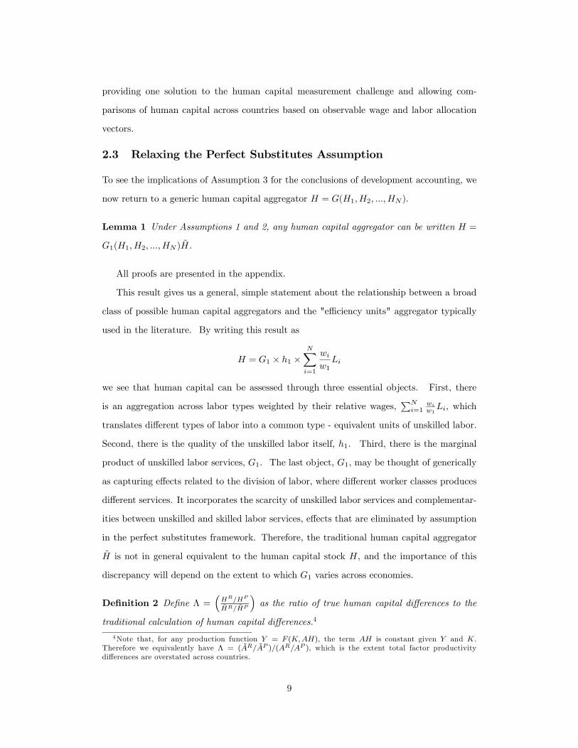
2.3 Relaxing the Perfect Substitutes Assumption

To see the implications of Assumption 3 for the conclusions of development accounting, we

now return to a generic human capital aggregator = (12 ).

Lemma 1 Under Assumptions 1 and 2, any human capital aggregator can be written =

1(12 ).

All proofs are presented in the appendix.

This result gives us a general, simple statement about the relationship between a broad

class of possible human capital aggregators and the "efficiency units" aggregator typically

used in the literature. By writing this result as

= 1 × 1 ×X=1

1

we see that human capital can be assessed through three essential objects. First, there

is an aggregation across labor types weighted by their relative wages,P

=11

, which

translates different types of labor into a common type - equivalent units of unskilled labor.

Second, there is the quality of the unskilled labor itself, 1. Third, there is the marginal

product of unskilled labor services, 1. The last object, 1, may be thought of generically

as capturing effects related to the division of labor, where different worker classes produces

different services. It incorporates the scarcity of unskilled labor services and complementar-

ities between unskilled and skilled labor services, effects that are eliminated by assumption

in the perfect substitutes framework. Therefore, the traditional human capital aggregator

is not in general equivalent to the human capital stock , and the importance of this

discrepancy will depend on the extent to which 1 varies across economies.

Definition 2 Define Λ =³

´as the ratio of true human capital differences to the

traditional calculation of human capital differences.4

4Note that, for any production function = (), the term is constant given and .

Therefore we equivalently have Λ = ( )( ), which is the extent total factor productivity

differences are overstated across countries.

9

It follows immediately from Lemma 1 (i.e. only on the basis of Assumptions 1 and 2)

that

Λ = 1

1

indicating the bias induced by the efficiency units approach.

This bias may be substantial. Moreover, there is reason to think that Λ ≥ 1; i.e., thatthe perfect-substitutes assumption will lead to a systematic understatement of true human

capital differences. To see this, note that 1 is likely to be substantially larger in a rich

country than a poor country, for two reasons. First, rich countries have substantially fewer

unskilled workers, a scarcity that will tend to drive up the marginal product of unskilled

human capital (11 0). Second, rich countries have substantially more highly educated

workers, which will tend to increase the productivity of the unskilled workers to the extent

that highly skilled workers have some complementarity with low skilled workers (1 6=1 0).

It will follow under fairly mild conditions that Λ ≥ 1. One set of conditions is as follows.

Lemma 2 Consider the class of human capital aggregators = (1 (2 )) with

finite and strictly positive labor services, 1 and . Under Assumptions 1 and 2, Λ ≥ 1 iff

1 ≥ 1 .

Thus, under fairly broad conditions, traditional human capital estimation provides only

a lower bound on human capital differences across economies.

2.3.1 A Generalized Estimation Strategy

In practice, the extent to which human capital differences may be understated depends on

the human capital aggregator employed as an alternative to the efficiency units specifica-

tion. Here we develop an alternative that (i) can be easily estimated and (ii) nests many

approaches, as follows.

Lemma 3 Consider the class of human capital aggregators = (1 (2 )).

If such an aggregator can be inverted to write (2 ) = (1), then the human

capital stock can be estimated solely from information about 1, , and production function

parameters.

This result suggests that there may be a broad class of aggregators that are relatively

easy to estimate, with the property that the aggregation of skilled labor, (23 ),

10

need not be measured directly. Moreover, any aggregator that meets the conditions of this

Lemma also meets the conditions of Lemma 2. Therefore, in comparison to traditional

human capital accounting, any such aggregator allows only greater human capital variation

across countries.

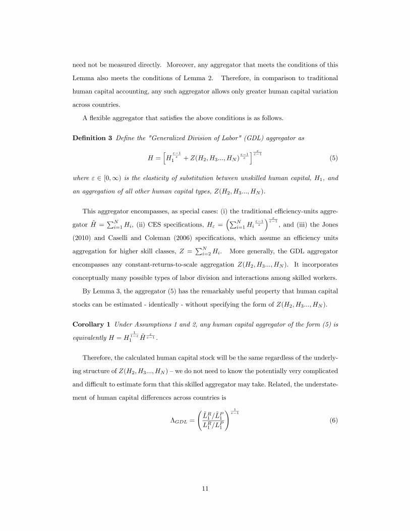
A flexible aggregator that satisfies the above conditions is as follows.

Definition 3 Define the "Generalized Division of Labor" (GDL) aggregator as

=h

−1

1 + (23)−1

i −1

(5)

where ∈ [0∞) is the elasticity of substitution between unskilled human capital, 1, and

an aggregation of all other human capital types, (23 ).

This aggregator encompasses, as special cases: (i) the traditional efficiency-units aggre-

gator =P

=1, (ii) CES specifications, =³P

=1

−1

´ −1, and (iii) the Jones

(2010) and Caselli and Coleman (2006) specifications, which assume an efficiency units

aggregation for higher skill classes, =P

=2. More generally, the GDL aggregator

encompasses any constant-returns-to-scale aggregation (23 ). It incorporates

conceptually many possible types of labor division and interactions among skilled workers.

By Lemma 3, the aggregator (5) has the remarkably useful property that human capital

stocks can be estimated - identically - without specifying the form of (23 ).

Corollary 1 Under Assumptions 1 and 2, any human capital aggregator of the form (5) is

equivalently = 1

1−1

−1 .

Therefore, the calculated human capital stock will be the same regardless of the underly-

ing structure of (23 ) — we do not need to know the potentially very complicated

and difficult to estimate form that this skilled aggregator may take. Related, the understate-

ment of human capital differences across countries is

Λ =

Ã1

1

1 1

! 1−1

(6)

11

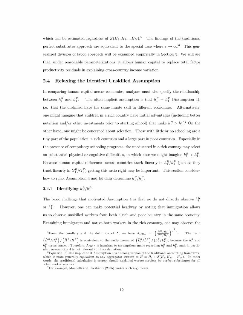
which can be estimated regardless of (23 ).5 The findings of the traditional

perfect substitutes approach are equivalent to the special case where → ∞.6 This gen-

eralized division of labor approach will be examined empirically in Section 3. We will see

that, under reasonable parameterizations, it allows human capital to replace total factor

productivity residuals in explaining cross-country income variation.

2.4 Relaxing the Identical Unskilled Assumption

In comparing human capital across economies, analyses must also specify the relationship

between 1 and 1 . The often implicit assumption is that 1 = 1 (Assumption 4),

i.e. that the unskilled have the same innate skill in different economies. Alternatively,

one might imagine that children in a rich country have initial advantages (including better

nutrition and/or other investments prior to starting school) that make 1 1 .7 On the

other hand, one might be concerned about selection. Those with little or no schooling are a

tiny part of the population in rich countries and a large part in poor countries. Especially in

the presence of compulsory schooling programs, the uneducated in a rich country may select

on substantial physical or cognitive difficulties, in which case we might imagine 1 1 .

Because human capital differences across countries track linearly in 1 1 (just as they

track linearly in 1

1 ) getting this ratio right may be important. This section considers

how to relax Assumption 4 and let data determine 1 1 .

2.4.1 Identifying 1 1

The basic challenge that motivated Assumption 4 is that we do not directly observe 1

or 1 . However, one can make potential headway by noting that immigration allows

us to observe unskilled workers from both a rich and poor country in the same economy.

Examining immigrants and native-born workers in the rich economy, one may observe the

5From the corollary and the definition of Λ, we have Λ =

1

1

1−1

. The term

1

1

is equivalent to the easily measured

1

1

1

1

, because the 1 and

1 terms cancel . Therefore, Λ is invariant to assumptions made regarding 1 and 1 , and, in partic-

ular, Assumption 4 is not relevant to this calculation.6Equation (6) also implies that Assumption 3 is a strong version of the traditional accounting framework,

which is more generally equivalent to any aggregator written as = 1 + (23 ). In other

words, the traditional calculation is correct should unskilled worker services be perfect substitutes for all

other worker services.7For example, Manuelli and Sheshadri (2005) makes such arguments.

12

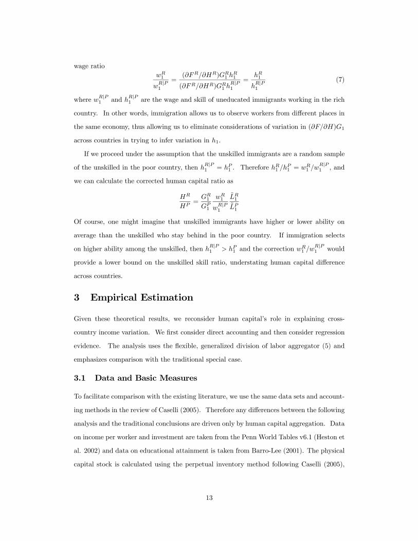
wage ratio

1

|1

=()

1 1

()1

|1

=1

|1

(7)

where |1 and

|1 are the wage and skill of uneducated immigrants working in the rich

country. In other words, immigration allows us to observe workers from different places in

the same economy, thus allowing us to eliminate considerations of variation in ()1

across countries in trying to infer variation in 1.

If we proceed under the assumption that the unskilled immigrants are a random sample

of the unskilled in the poor country, then |1 = 1 . Therefore 1

1 =

1 |1 , and

we can calculate the corrected human capital ratio as

=

1

1

1

|1

1

1

Of course, one might imagine that unskilled immigrants have higher or lower ability on

average than the unskilled who stay behind in the poor country. If immigration selects

on higher ability among the unskilled, then |1 1 and the correction

1 |1 would

provide a lower bound on the unskilled skill ratio, understating human capital difference

across countries.

3 Empirical Estimation

Given these theoretical results, we reconsider human capital’s role in explaining cross-

country income variation. We first consider direct accounting and then consider regression

evidence. The analysis uses the flexible, generalized division of labor aggregator (5) and

emphasizes comparison with the traditional special case.

3.1 Data and Basic Measures

To facilitate comparison with the existing literature, we use the same data sets and account-

ing methods in the review of Caselli (2005). Therefore any differences between the following

analysis and the traditional conclusions are driven only by human capital aggregation. Data

on income per worker and investment are taken from the Penn World Tables v6.1 (Heston et

al. 2002) and data on educational attainment is taken from Barro-Lee (2001). The physical

capital stock is calculated using the perpetual inventory method following Caselli (2005),

13

and unskilled labor equivalents are calculated using data on the wage return to schooling.

These data methods are further described in the appendix.

Again following the standard literature, we will use Cobb-Douglas aggregation, =

()1− and take the capital share as = 13. Writing = 1− to account

for the component of income explained by measurable factor inputs, Caselli (2005) defines

the success of a factors-only explanation as

=

where is a "rich" country and is a "poor" country. We will denote the success measure

for traditional accounting, based on , as .

3.2 Accounting Evidence

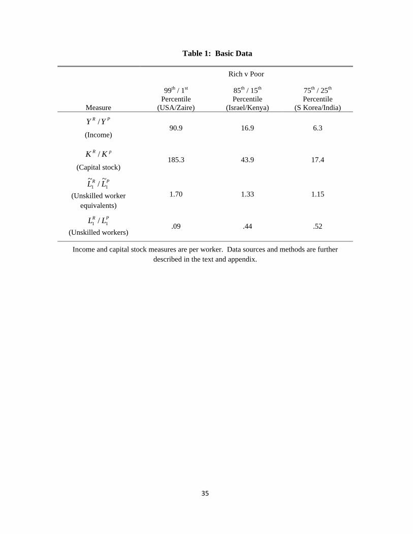
Table 1 summarizes some basic data. Comparing the richest and poorest countries in the

data (the USA and Congo-Kinshasa), the observed ratio of income per-worker is 91. The

capital ratio is larger, at 185, but the ratio of unskilled labor equivalents is much more

modest, at 17. Comparing the 85th to 15th percentile (Israel and Kenya) or the 75th to

25th percentile (S. Korea and India), we again see that the ratio of income and physical

capital stocks is much greater than the ratio of unskilled labor equivalents.

Using unskilled labor equivalents to measure human capital stock variation, it follows

that = 45% comparing Korea and India, = 25% comparing Israel and

Kenya, and = 9% when comparing the USA to the Congo. These calculations sug-

gest that large residual productivity variation is needed to explain the wealth and poverty of

nations. These findings rely on unskilled labor equivalents, 1 1 , to measure human cap-

ital stock variation. Because unskilled labor equivalents vary little, human capital appears

to add little to explaining productivity differences.8

3.2.1 Relaxing the Perfect-Substitutes Assumption

The relationship between the traditional success measure and the success measure for a

general human capital aggregator is

= Λ1− ×

8Figure A1 shows when comparing all income percentiles from 70/30 (Malaysia/Honduras) to

99/1 (USA-Congo). The average measure of is 31% over this sample.

14

which follows from Lemma 1 and the definition of Λ.

One can implement a generalized accounting using the GDL aggregator. From (6) and

the data in Table 1, it is clear that Λ can be large. While the variation in unskilled labor

equivalents, 1 1 , is modest, the human capital variation that corrects for labor division

expands according to two objects. One is the relative scarcity of unskilled labor services,

1 1 . The second is the degree of complementarity between skilled and unskilled labor

services, as defined by .

The literature on the elasticity of substitution between skilled and unskilled labor within

countries suggests that ∈ [1 2].9 Table 2 (Panel A) reports the results of development

accounting over this range of , focusing on the Israel-Kenya example. The first row

presents the human capital differences, , the second row presents the ratio of these

differences to the traditional calculation, Λ, and the third row presents the resulting

measure for capital inputs in explaining cross-country income differences. As shown

in the table, factor-based explanations for income differences are substantially amplified by

allowing for labor division. As complementarities across workers increase, the need for TFP

residuals decline.10 For the Israel-Kenya example, the need for residual TFP differences is

eliminated at = 154, where human capital differences are = 105.

One can also consider a broader set of rich-poor comparisons; for example, all coun-

try comparisons from the 70/30 income percentile (Malaysia/Honduras) up to the 99/1

percentile (USA/Congo).11 Calculating the elasticity of substitution, , at which capital

inputs fully explain income differences, shows that the mean value is = 155 in this sample

with a standard deviation of 034. Notably, the estimated values of typically fall in the

same [1 2] interval as the micro-literature suggests.

9See, e.g. reviews in Katz and Autor (1999) and Ciccone and Peri (2005). Most estimates come from

regression analyses that may be substantially biased due to the endogeneity of labor supply. Ciccone and

Peri (2005) use compulsory schooling laws as a source of plausibly exogenous variation in schooling across

U.S. states and find that is in a range between 13 and 2 depending on the specification. All these

estimates consider the elasticity of substitution between high-school and college-educated workers, and they

may not extend to primary vs non-primary educated workers. The regression analysis below, however, also

suggests in this range.10The intuition for this result will be discussed in Section 4.11The Malaysia/Honduras income ratio is 3.8. As income ratios (and capital measures) converge towards

1, estimates of become noisier.

15

3.2.2 Relaxing the Identical Unskilled Assumption

Table 2 (Panel B) further relaxes Assumption 4, allowing 1 1 to be determined from

immigration data. Examining immigrants to the U.S. using the year 2000 U.S. Census, the

mean wages of employed unskilled workers varies modestly based on the source country (see

Figure A2). While the data are noisy, one may infer that mean wages are about 17% lower

for uneducated workers born in the U.S. compared to immigrants from the very poorest

countries, which suggests 1 1 ≈ 83 (see Appendix for details).12

Such an adjustment lowers the explanatory power of human capital in explaining cross-

country variation. The adjustment seems large - it cuts human capital differences by

17%. However, in practice, relaxing Assumption 4 has modest effects compared to relaxing

Assumption 3, as seen in Table 2. Now residual TFP differences are eliminated when

= 150 for the Israel-Kenya comparison. Across the broader set of rich-poor examples,

additionally relaxing Assumption 4 leads to a mean value of = 158, with a standard

deviation of 037.

The human capital stock estimations are summarized for the broader sample in Figure

2. The ratio of human stocks for each pair of countries from the 70/30 income percentile

to the 99/1 income percentile is presented. Panel A considers the generalized framework,

with = 16. Panel B considers traditional human capital accounting. We see that, as

reflected in Table 1, traditional human capital accounting admits very little human capital

variation. It appears orders of magnitude less than the variation in physical capital or

income. With the generalized framework, human capital differences substantially expand,

admitting variation similar in scale to the variation in income and physical capital.

3.3 Regression Evidence

Regression analysis in the development accounting context is controversial. While Mankiw,

Romer, and Weil (1992) find a large 2 and theoretically credible relationships between

capital aggregates and output, Klenow and Rodriguez-Clare (1997) point out the omitted

12This micro-data finding stands in contrast to the cross-country analysis of Manuelli and Seshadri (2005),

which relies on 1 1 . Manuelli and Seshadri (2005) can be understood as relaxing Assumption 4 but

not relaxing Assumption 3, which means that one will require 1 1 to increase the explanatory power

of human capital in a cross-country setting. The immigrant wage data is inconsistent with 1 1unless one assumes that uneducated immigrants to the U.S. select on extremely high ability compared to

the non-immigrating population. More generally, Table 2 suggests that much more action comes from

relaxing Assumption 3.

16

variable hazards in interpreting such regressions. In practice, because average schooling is

highly correlated with income per-capita, regressions of income on schooling variables will

tend to show highly significant positive relationships and large 2. While this correlation

might be causative, it may well not be, and caution is needed.13

Given these concerns, the more telling aspect of regression analysis may come less from

high 2 and more from the implied production function parameters. In particular, it

is informative whether the estimated production function parameters are consistent with

the production functions being estimated in direct accounting exercises. This connection

explicitly fails in the traditional analyses: using a (quasi14) perfect substitutes aggregation

of human capital, Mankiw, Romer, Weil (1992) suggests that human capital plays a primary

role in cross-country income differences, but explicit accounting using a perfect substitutes

aggregation suggests the opposite conclusion.

In this section, we show that the generalized aggregator may avoid this conflict. Con-

tinuing with the standard Cobb-Douglas production function, = ()1−, define

income net of physical capital’s contribution as log = log − log. The GDL ag-

gregator implies log = (1 − )[log + 11− log1 +

−1 log ]. A regression can then

estimate

log = 0 + 1 log1 + 2 log

+ (8)

where indexes countries. The values of are then implied by the coefficient estimates.15

3.3.1 Relaxing the Efficiency Units Assumption

Table 3 presents the regression results. Columns (1)-(3) examine (8) while maintaining

Assumption 4. Column (1) shows that the explanatory power of log is substantial. The

coefficient implies = 134, with a 95% confidence interval of [128 134]. Column (2)

considers the explanatory power of log1, which is also substantial. The coefficient implies

13An additional challenge for the original Mankiw, Romer, and Weil (1992) approach is the linear use of

schooling duration for the human capital aggregator, i.e. =

=1 , where is the number of years

of school. This approach is an efficiency units aggregator (Assumption 3) combined with an additional

assumption equating skill to years in school, i.e. = . However, this combination is inconsistent with

the wage evidence. Under Assumption 3, the relative skill is linear in the relative wage, ,

which are log-linear in schooling duration, not linear. Thus the assumption that = does not appear

supportable with a neoclassical aggregator.14 See prior footnote.15Regression estimates that attempt to account for both physical and human capital simultaneously

are much noisier, presumably due to the high correlation between these capital stocks and consequent

multicollinearity.

17

= 170, with a 95% confidence interval of [150 217]. Considering log and log1

together, in column (3), the estimates of rise somewhat and become noisier.

3.3.2 Relaxing the Identical Unskilled Assumption

Table 3 columns (4)-(6) further examine (8) while additionally relaxing Assumption 4. Im-

migrant wage outcomes are used to estimate variation in 1 from the U.S. 2000 census, and

the measures for log and log1 are then adjusted accordingly. (The methodology is

further detailed in the Appendix.) In column (4) the coefficient on log now implies

= 164, with a 95% confidence interval of [150 187]. In column (5) the coefficient on

log1 implies = 188, with a 95% confidence interval of [164 238]. Joint estimation

again raises the estimates somewhat and expands the confidence intervals. Many robust-

ness checks have also been considered, varying how and 1 are calculated, as further

discussed in the Appendix. In general, the regressions tend to point to estimates of in

similar ranges.

Overall, we see broad consistency between (1) the range of that eliminates TFP dif-

ferences in explicit accounting, (2) regression estimates of , and (3) within-country micro-

evidence on the substitutability between skilled and unskilled labor. These observations

suggest that the GDL aggregator may provide a reasonable theoretical approach, resolving

the tension between regression and accounting methodologies while implying that human

capital variation can now play a substantial role in explaining income variation across coun-

tries. These findings - both Table 2 and Table 3 - are robust to any constant-returns-to-scale

specification of the aggregator (23 ).

4 Inside Human Capital Stocks

A value of the human capital stock calculations above is that they do not require detailed

specification of the aggregator. At the same time, it would be useful to look "underneath

the hood" and gain a better understanding of where the variation in stocks may come from.

One basic question is whether the increased human capital services in rich countries follow

from the quantity and/or quality of skilled labor. It is clear (Figure 1), that the quantity of

skilled laborers is much greater in rich countries. It will be shown below that the quality of

skilled laborers also appears much greater in rich countries. An ensuing question is then how

18

quality advantages in rich countries may emerge, and the greater acquisition of knowledge

by skilled workers will be offered as a potential explanation. While empirical estimation

becomes increasingly challenging, given the lack of consensus (or knowledge) about produc-

tion functions at this level of detail, the theory provides a road-map for estimation, and

illustrative calibrations are offered.

4.1 The Quality and Quantity of Labor Services

We begin with theoretical considerations for inferring labor quality. In general under

Assumptions 1 and 2, the relative "quality" of two groups of laborers in an economy is,

from (3)

=

(9)

where = is the mean flow of services from the workers in group . Thus the relative

qualities () can in general be inferred from relative wages (), which are factor

prices, and the relative marginal products of the human capital intermediates (),

which are the relative prices of the human capital services.

Now consider a type of partial equilibrium experiment, where we hold the relative prices

() fixed. In that case, increasing the skill ratio by a factor of would increase

the wage ratio by the same factor. This provides standard intuition, for example, for the

common practice in economics of using wage returns to schooling variation to make claims

about variation in skill returns. Were we to extend such reasoning to comparisons between

rich and poor countries, we would infer the relative quality of labor services asÃ

!

=

(10)

where the subscript "PE" indicates that we are using a type of partial equilibrium reasoning.

Of course, comparing economies with substantially different factor allocations suggests

that partial equilibrium analysis could be problematic. In general equilibrium, we need to

introduce the possibility that relative prices () vary.16 This caution becomes more

precise by allowing for the labor allocation to shift in response to variations in skill returns.

16 Ignoring such price variation in general equilibrium requires Assumption 3 — that different skill classes

are perfect substitutes — so that is a constant. However, as discussed above, perfect substitutability

across educational groups appears inconsistent with the empirical evidence (e.g., Katz and Autor 1999,

Ciccone and Peri 2005).

19

To see this, consider a simple stylized theory with endogenous labor supply.17

Assumption 5 Let individual income, , as a function of educational duration, , be

() =R∞

()− where the discount rate is fixed. Let individuals be identical

ex-ante and maximize income with respect to educational duration.

Workers train for some period of years and then work, with choices over training duration

determining the supply of various worker classes. Defining an elasticity of substitution

= − ln()

ln(), we establish the following result.

Lemma 4 Under Assumptions 1, 2, and 5, (a) ln()

ln()= 0 and (b)

ln()

ln()= −1.

This result provides exactly the opposite intuition from the partial equilibrium reasoning.

Namely, the lemma says that quality variation will appear through quantities, not through

wages. If labor supply is endogenous as in Assumption 5, then labor allocations shift to

neutralize the wage variation. Under the lemma, and comparing two countries with a

common discount rate, we have the general equilibrium counterpoint to (10)Ã

!

=

(11)

With endogenous labor supply, quality variation becomes divorced from wage variation and

appears instead through the allocative shifts that the partial equilibrium reasoning ignored.

To further establish this general equilibrium intuition, and its empirical relevance, con-

sider the following observation (and see Figure 3 below). Skilled-unskilled wage ratios tend

to be fairly similar across economies, while skilled-unskilled labor supply ratios tend to be

extremely different. That wage returns to education are fairly similar across economies fol-

lows naturally from result (a) of the lemma; when labor supply is endogenous, equilibrium

investment levels in education drive the rate of return to the local discount rate. How

then can a country like the United States sustain high wage returns to education despite a

massive increase in the quantity of highly-educated workers? Quality advantages provide

an answer. Expanded labor supply lowers the prices for skilled labor services. To maintain

such labor supply in equilibrium, one needs quality advantages.

17The educational choice decision follows Mincer’s original theoretical justification for the log-linear wage-

schooling relationship (Mincer 1958). The assumption that is fixed could be relaxed. See also Jones

(2010).

20

The lemma also makes this quantity-quality linkage explicit, via result (b). When the

elasticity of substitution between skilled and unskilled labor is greater than one, economies

with higher skilled quality will see greater skilled labor supply in response. Moreover, for a

given difference in labor quantity, the implied quality differences become increasingly large as

the elasticity of substitution falls toward one (because skilled output prices fall increasingly

quickly in response to skilled quantity increases, so that larger quality differences are required

to maintain the wage ratio). This theoretical reasoning explains why, in Table 2, human

capital’s capacity to explain cross-country income differences is increasing as the elasticity

of substitution falls.

4.1.1 Empirical Estimates of Quality Differences

Figure 3 presents the variation in wage returns and skilled labor supply when comparing rich

and poor countries. Defining as the mass of skilled workers and as their mean wage,

the variation in wage returns is seen to be exceptionally modest, while the variation in labor

supply is enormous. Taking the Israel-Kenya example, the relative skilled labor allocation

(1) is 2300% greater in Israel, while the wage returns (1) are only 20% lower.

Taking the USA-Congo example, the relative skilled labor allocation is 17500% greater in

the USA, while the wage returns are only 15% lower. Consistent with Lemma 4, massive

increases in skilled labor supply can be reconciled with little if any drop in wage returns

through variation in the quality of skilled labor services.

To estimate the variation in the quality of skilled services, return first to the human

capital stock calculations of Section 3. Using the GDL aggregator in tandem with (9), one

can infer the skilled-unskilled ratio of mean service flows as

1

1

=

µ

1

1

¶ −1 µ 1

1

¶ 1−1

(12)

where = (23 ) is the mean flow of services from skilled workers.

Table 4 (Panel A) reports the implied variation in 1, continuing with the rich-poor

example in Table 2. Recall that human capital stock variation eliminates residual total

factor productivity variation when ≈ 16. At this value of , the relative service flows

of skilled workers in the rich country appear 986 times larger than in the poor country.

This empirical finding is consistent with Caselli and Coleman (2006), but now explicitly

extended to the general class of skilled labor aggregators, (23 ). Thus similar

21

wage returns are consistent with massive differences in labor allocation when skilled service

flows are substantially higher in rich countries.

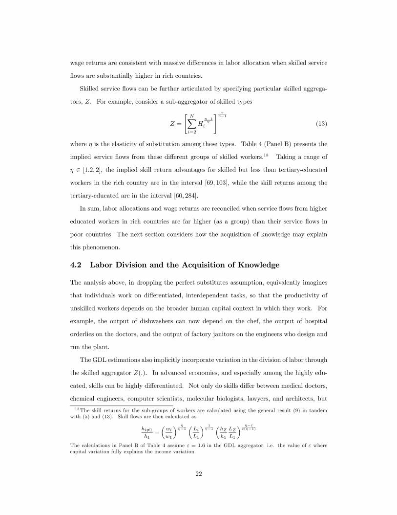
Skilled service flows can be further articulated by specifying particular skilled aggrega-

tors, . For example, consider a sub-aggregator of skilled types

=

"X=2

−1

# −1

(13)

where is the elasticity of substitution among these types. Table 4 (Panel B) presents the

implied service flows from these different groups of skilled workers.18 Taking a range of

∈ [12 2], the implied skill return advantages for skilled but less than tertiary-educatedworkers in the rich country are in the interval [69 103], while the skill returns among the

tertiary-educated are in the interval [60 284].

In sum, labor allocations and wage returns are reconciled when service flows from higher

educated workers in rich countries are far higher (as a group) than their service flows in

poor countries. The next section considers how the acquisition of knowledge may explain

this phenomenon.

4.2 Labor Division and the Acquisition of Knowledge

The analysis above, in dropping the perfect substitutes assumption, equivalently imagines

that individuals work on differentiated, interdependent tasks, so that the productivity of

unskilled workers depends on the broader human capital context in which they work. For

example, the output of dishwashers can now depend on the chef, the output of hospital

orderlies on the doctors, and the output of factory janitors on the engineers who design and

run the plant.

The GDL estimations also implicitly incorporate variation in the division of labor through

the skilled aggregator (). In advanced economies, and especially among the highly edu-

cated, skills can be highly differentiated. Not only do skills differ between medical doctors,

chemical engineers, computer scientists, molecular biologists, lawyers, and architects, but

18The skill returns for the sub-groups of workers are calculated using the general result (9) in tandem

with (5) and (13). Skill flows are then calculated as

6=11

=

1

−1

1

1−1

1

1

−(−1)

The calculations in Panel B of Table 4 assume = 16 in the GDL aggregator; i.e. the value of where

capital variation fully explains the income variation.

22

skills within professions can be highly differentiated themselves. For example, there are

145 accredited medical specialities in the United States, and MIT offers 119 courses across

8 sub-specialities within aeronautical engineering alone.19 By comparison, Uganda has 10

accredited medical specialties, and the engineering faculty of Mekerere University, often

rated as the top university in Sub-Saharan Africa outside South Africa, does not offer any

aeronautics courses within its engineering curriculum.

This section considers greater task specialization among skilled workers as a possible

explanation for the greater skilled service flows in rich countries. The approach incorporates

the classic idea that the division of labor may be a primary source of economic prosperity

(e.g., Smith 1776) and builds on ideas in a related paper (Jones 2010), which considers

micro-mechanisms that can obstruct collective specialization among skilled workers.

The core observation is that focused training and experience can provide extremely

large skill gains at specific tasks. For example, the willingness to pay a thoracic surgeon

to perform heart surgery is likely orders of magnitude larger than the willingness to pay a

dermatologist (or a Ph.D. economist!) to perform that task. Similarly, when building a

microprocessor fabrication plant, the service flows from appropriate, specialized engineers

are likely orders of magnitude greater than could be achieved otherwise. Put another way,

if no individual can be an expert at everything, then embodying the stock of productive

knowledge in the workforce requires a division of labor. Possible limits to task specialization

include: (i) the extent of the market (e.g. Smith 1776); (ii) coordination costs across workers

(e.g. Becker and Murphy 1992); (iii) the extent of existing advanced knowledge (Jones 2009);

and (iv) local access to advanced knowledge (e.g. Jones 2010). Here we consider a simple

production theory to explore how variation in task specialization may explain variation in

skilled services across economies.20

4.2.1 Production with Specialized Skills

Consider skilled production as the performance of a wide range of tasks, indexed over a

unit interval. Production can draw on a group of individuals. With individuals, each

member of the group can focus on learning an interval 1 of the tasks. This specialization

19Accredited medical specialities are listed by the American Board of Medical Special-

ties, http://www.abms.org. The MIT subject offerings are found in the MIT Bulletin,

http://web.mit.edu/catalog/.20The following set-up is closest theoretically to Becker and Murphy (1992) and Jones (2010). It differs

in part by providing a path toward calibration.

23

allows the individual to focus her training on a smaller set of tasks, increasing her mastery

at this set of tasks. If an individual devotes a total of units of time to learning, then the

time spent learning each task is .

Let the skill at each task be defined by a function () where 0() 0. Meanwhile, let

there be a coordination penalty () for working in a team. Let task services aggregate with

a constant returns to scale production function that is symmetric in its inputs, so that the

per-capita output of a team of skilled workers with breadth 1 will be ( ) = ()().

We assume that 0() 0, so that bigger teams face larger coordination costs, acting to

limit the desired degree of specialization.21

Next consider the choice of and that maximizes the discounted value of skilled services

per-capita.22 This maximization problem is

max

Z ∞

( )−

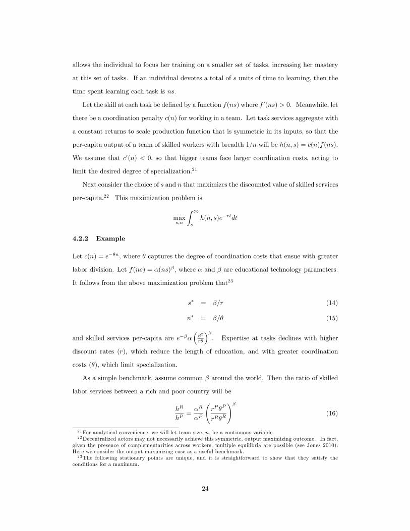
4.2.2 Example

Let () = −, where captures the degree of coordination costs that ensue with greater

labor division. Let () = () , where and are educational technology parameters.

It follows from the above maximization problem that23

∗ = (14)

∗ = (15)

and skilled services per-capita are −³2

´. Expertise at tasks declines with higher

discount rates (), which reduce the length of education, and with greater coordination

costs (), which limit specialization.

As a simple benchmark, assume common around the world. Then the ratio of skilled

labor services between a rich and poor country will be

=

Ã

!

(16)

21For analytical convenience, we will let team size, , be a continuous variable.22Decentralized actors may not necessarily achieve this symmetric, output maximizing outcome. In fact,

given the presence of complementarities across workers, multiple equilibria are possible (see Jones 2010).

Here we consider the output maximizing case as a useful benchmark.23The following stationary points are unique, and it is straightforward to show that they satisfy the

conditions for a maximum.

24

This model thus suggests a complementarity of mechanisms. Differences in the quality of

education (), discount rates (), and coordination penalties () have multiplicative effects.

These interacting channels provide compounding means by which skilled labor services may

differ substantially across economies.

4.2.3 Calibration Illustration

We focus on the division of labor. Note from (15) that with common the equilibrium

difference in the division of labor (that is, the team size ratio) is equivalent to the inverse

coordination cost ratio, . To calibrate the model, let = 22, which follows if the

duration of schooling among the highly educated is 22 years and the discount rate is 01.

Further let = 1 and take the Mincerian coefficients as those used to calculate each

country’s human capital stocks throughout the paper, as described in the Appendix. Figure

4 then plots the implied variation in the division of labor, , that reconciles (16) with

the quality variation implied by (12), under the assumption that rich countries have

no advantage in education technology.

We find that a 4.3-fold difference in the division of labor can explain the productivity

difference between Israel and Kenya (the 85-15 percentile country comparison), and a 2.4-fold

difference explains the productivity difference between Korea and India (the 75-25 percentile

country comparison). The extreme case of the USA and the former Zaire is explained with a

22-fold difference. These differences would fall to the extent that the education technology

(,) is superior in richer countries.

Are large division of labor differences reasonable? Systematic measures are not readily

available in the micro-literature and await further research, but the anecdotes above about

medical and engineering specialization do suggest very large differences, and specialized

training clearly raises skills at particular tasks by very large multiples. In any case, the

primary observation here is that considerations of task specialization face little theoretical

constraint in providing an interpretation for both (1) the large differences in skilled labor

allocations across countries and (2) the large differences in human capital stocks estimated

in this paper.

25

5 Discussion

5.1 Summary

This paper introduces a generalized framework for human capital accounting. Traditional

development accounting is nested as a special case and, under mild conditions, is shown to

provide only a lower bound on human capital variation across economies. A "generalized

division of labor" aggregator is introduced, which allows human capital stocks to be calcu-

lated with relatively little aggregation structure. This framework can reconcile the conflict

between regression analyses (e.g. Mankiw, Romer, and Weil 1992) and traditional account-

ing approaches (e.g. Klenow and Rodriguez-Clare 1997, Hall and Jones 1999, Caselli 2005).

Human capital stocks can now play a central role in explaining the wealth and poverty of

nations.

Having established these results about human capital stocks, the paper further considers

possible underlying sources of human capital variation. First, the generalized framework

is extended to account for quality differences in workers’ service flows. Wage variation is

found to be a poor guide to quality differences, because labor supply adjustments tend to

neutralize the wage effects. In consequence, quality differences tend to appear as quantity

differences rather than wage differences. Because skilled labor quantity differences are so

large across countries, one infers correspondingly large differences in skilled labor qualities.

Second, variation in knowledge acquisition is incorporated into the accounting framework.

Increased specialization — allowing greater collective acquisition of knowledge — is seen to

amplify skilled service flows, providing a candidate, underlying production theory for the

relatively large quality of skilled worker services in advanced economies.

5.2 Interpretations, Implications, and Extensions

The paper’s estimates of human capital stocks suggest that cross-country output variation

can now be accounted for without relying on residual, total factor productivity (TFP) vari-

ation. Because TFP is often interpreted as (i) "ideas" and/or (ii) "institutions", this paper

might therefore seem to diminish these explanations for economic development. Such an

implication, however, need not follow if (1) ideas are embodied in the capital inputs and (2)

the embodiment process is influenced by institutions. In this interpretation, the contribution

of this paper is not in reducing the roles of ideas or institutions, but in emphasizing human

26

capital’s potential as a central feature of understanding productivity differences. This paper

closes by considering this perspective.

Consider ideas first. Macroeconomic arguments aside, studies of actual production

processes through history suggest that the creation and diffusion of ideas are central to

understanding productivity.24 Yet one may also claim, by studying any particular pro-

duction process, that ideas enter production only when they are known and implemented;

that is, only when actuated through tangible inputs - the people and their physical inputs

that actually make things. In fact, the physical instantiation of an idea may be a good

description of what physical capital is (e.g. a microprocessor is a set of ideas etched on

silicon) and learning ideas may be a good description of education (e.g. skilled workers are

vessels of facts, theories, and techniques). In this view, one doesn’t need TFP for ideas to

be a centerpiece of economic development.

Putting ideas into production through capital inputs, rather than as a residual, also pro-

vides explicit processes in which institutions matter. As further emphasized by the division

of labor model, individuals may collectively fail to embody advanced ideas when faced, e.g.,

with high interest rates, high coordination costs, and poor educational institutions. Institu-

tional features like credit constraints, weak property rights and contracting environments,

and poor public good provision would then naturally underpin these investment failures.

Lastly, claiming that ideas enter production through people and their machines leads

quickly to an emphasis on the division of labor. If embodiment is needed for ideas to

become useful in production, then this next logical step follows to the extent that the set

of existing ideas is too large for any one person to know. Differentiated knowledge across

workers is then necessary to bring the collective set of advanced ideas into production (Jones

2009). Thus, while the division of labor calibration in Section 5 provides one approach, the

broader point is that successfully mapping an advanced economy’s ideas into productive

inputs naturally depends on specialized workers, which suggests that the division of labor

is a central aspect of understanding human capital and economic development. Jones

(2010) further develops this idea and suggests that, beyond cross-country income differences,

division of labor variation can explain a variety of stylized facts about the world economy.

24See, e.g., Mokyr’s The Lever of Riches (1992) for many historical examples. Nordhaus (1997) provides

a powerful example by studying the price of light through time. Conley and Udry (2010) is one of many

studies demonstrating that ideas can fail to diffuse in poor countries.

27

In summary, the analysis in this paper suggests a substantially amplified role of human

capital. The findings offer a reconciliation of regression and accounting approaches to human

capital measurement. More broadly, the findings are fully consistent with a framework in

which investment, ideas, and institutions play substantive roles — but where human capital

is drawn to the heart of economic development.

While the framework is applied here to cross-country income differences, the same frame-

work has other natural applications at the level of countries, regions, cities, or firms. Growth

accounting provides one direction for future work. The urban-rural economy literature is

another direction, where productivity differences from specialization are often suggested as

critical but cannot be captured using traditional human capital measures.

28

6 Appendix

Proof of Lemma 1

Proof. = (12 ) is constant returns in its inputs (Assumption 1). Therefore,

by Euler’s theorem for homogeneous functions, the true human capital aggregate can gener-

ically be written =P

=1. Rewrite this expression as = 11P

=111

.

Recalling that =

(Assumption 2), so that1=

11, we can therefore write

= 111, where 1 =P

=11

.

Proof of Lemma 2

Proof. If = (1 ) is constant returns to scale, then 1 is homogeneous of degree

zero by Euler’s theorem. Therefore 1(1 ) = 1(1 1). Noting that 11 ≤ 0, itfollows that Λ =

1 1 ≥ 1 iff

1 ≥ 1 .

Proof of Lemma 3

Proof. By Lemma 1, = 1, providing an independent expression for based

on its first derivative. If the human capital aggregator can be manipulated into the

form = (1 (2 )) = (1 (1)), then we have from Lemma 1 =

1(1 (1)). This provides an implicit function determining solely as a function

of 1 and ; that is, without reference to (2 ).

Proof of Corollary 1

Proof. By Lemma 1, = 1. For the GDL aggregator, 1 = (1)1 . Thus =

1

1−1

−1 .

Proof of Lemma 4

Proof. Consider two skill categories that require and years of training respectively.

Holding these durations fixed, imagine that the skill levels and associated with each

may vary. Assumptions 1 and 2 imply (3). Taking logs and differentiating, it follows that

1 = ln()

ln()+ 1

³1 +

ln()

ln()

´. Under Assumption 5, arbitrage in career choices

(() = ()) implies = (−). Thus, if labor supply is endogenous, then the

29

wage returns are pegged to the duration of training, not the skill associated with it. It then

follows that ln()

ln()= 0. Hence the result.

Data Appendix

Capital Stocks

To minimize sources of difference with standard assessments, this paper uses the same

data in Caselli’s (2005) review of cross-country income accounting. Income per worker is

taken from the Penn World Tables v6.1 (Heston et al. 2002) and uses the 1996 benchmark

year. Capital per worker is calculated using the perpetual inventory method, = +

(1 − )−1, where the depreciation rate is set to = 006 and the initial capital stock is

estimated as 0 = 0( + ). Further details are given in Section 2.1 of Caselli (2005).

As a robustness check, I have also considered calculating capital stocks as the equilibrium

value under Assumptions 1 and 2 with a Cobb-Douglas aggregator; i.e., = () , where

= 13 is the capital share and = 01. This alternative method provides similar results

as in the main paper.

To calculate human capital stocks, I use Barro and Lee (2001) for the labor supply

quantities for those at least 25 years of age, which are provided in five groups: no schooling,

some primary, completed primary, some secondary, completed secondary, some tertiary, and

completed tertiary. Schooling duration for primary and secondary workers are taken from

Caselli and Coleman (2006) and schooling duration for completed tertiary is assumed to be

4 years. Schooling duration for "some" education in a category is assumed to be half the

duration for complete education in that category.

For wage returns to schooling, I use Mincerian coefficients from Psacharopoulos (1994)

as interpreted by Caselli (2005). Let be the years of schooling and let relative wages be

() = (0). Psacharopoulos (1994) finds that wage returns per year of schooling are

higher in poorer countries, and Caselli summarizes these findings with the following rule.

Let = 013 for countries with ≤ 4, where = (1)P=1 is the country’s average

years schooling. Meanwhile, let = 010 for countries with 4 ≤ 8, and let = 007 forthe most educated countries with 8. Unskilled labor equivalents are then calculated as

1 =P

=1 in each country.

30

As a robustness check, I have considered calculating human capital stocks under a va-

riety of other assumptions. The results using the GDL aggregators are broadly robust to

reasonable alternative human capital input measures. The sample mean value of at which

capital stocks fully explain income variation typically falls in the the [15 2] interval across

human capital accounting methods. For example, if we set = 10 (the global average)

for all countries, then the gap between unskilled labor equivalents widens slightly, since the

returns to education in poor countries now appear lower and the returns in rich countries

appear higher. The resulting increase in human capital ratio means that capital inputs can

explain income differences at somewhat higher values of , but still with 2.

Variation in the Quality of Unskilled Labor

Following the analysis in Section 2.4, we estimate the difference in unskilled qualities as

1 1 =

1 |1 , where wages are for unskilled workers in the U.S. The term

1 is the

mean wage for unskilled workers born in the US and |1 is the mean wage for unskilled

workers born in a poor country and working in the US.

Wages are calculated from the 5% microsample of the 2000 U.S. Census (available from

www.ipums.org). Unskilled workers are defined as employed individuals with 4 or less years

of primary education (individuals with educ=1 in the pums data set) who are between the

ages of 20 and 65. To facilitate comparisons, mean wages are calculated for individuals who

speak English well (individuals with speakeng=3, 4, or 5 in the pums data set).

Figure A2 presents the data, with the mean wage ratio, |1

1 , plotted against log

per-capita income of the source country. (National income data is taken from the Penn

World Tables v6.1.) There is one observation per source country, but the size of the marker

is scaled to the number of observed workers from that source country. The figure plots the

results net of fixed effects for gender and each integer age in the sample.

For accounting and regression analysis when relaxing Assumption 4, the (weighted)

mean of 1

|1 is calculated for five groups of immigrants based on quintiles of average

schooling duration in the source country. The age and gender controlled data is used,

although using the raw wage means produces similar findings. The corrections for 1 1

are then applied to the human capital stock in each country. These corrected data are used

(only) when Assumption 4 is relaxed — in Panel B of Table 2, Figure 2B, and columns (4)-(6)

31

of Table 3. One can use other reasonable methods to calculate 1

|1 and apply it to

the human capital measures, but in general the primary findings of the paper are robust to

such variations, because the implications of relaxing Assumption 3 tend to be much greater.

References

[1] Banerjee, Abhijit and Esther Duflo. "Growth Theory Through the Lens of Development

Economics", The Handbook of Economic Growth, Aghion and Durlauf eds., Elsevier,

2005.

[2] Becker, Gary S. and Kevin M. Murphy. "The Division of Labor, Coordination Costs,

and Knowledge", Quarterly Journal of Economics, November 1992, 107 (4), 1137-1160..

[3] Caselli, Francesco. "Accounting for Cross-Country Income Differences", The Handbook

of Economic Growth, Aghion and Durlauf eds., Elsevier, 2005.

[4] Caselli, Francesco and Wilbur J. Coleman. "The World Technology Frontier", American

Economic Review, June 2006, 96 (3), 499-522.

[5] Conley, Timothy G. and Christopher R. Udry. "Learning About a New Technology:

Pineapple in Ghana", American Economic Review, March 2010, 100 (1), 35-69.

[6] Garicano, Luis. "Hierarchies and the Organization of Knowledge in Production", Jour-

nal of Political Economy, October 2000, 108 (5), 874-904.

[7] Hall, Robert and Charles Jones. "Why Do Some Countries Produce So Much More

Output Per Worker Than Others?", Quarterly Journal of Economics, February 1999,

114 (1), 83-116.

[8] Heckman, James J., Lochner, Lance J., and Petra E. Todd. "Earnings Functions: Rates

of Return and Treatment Effects: The Mincer Equation and Beyond", IZA Discussion

Paper Series No. 1700, August 2005.

[9] Hendricks, Lutz. "How Important Is Human Capital for Development? Evidence from

Immigrant Earnings", American Economic Review, March 2002, 92 (1), 198-219.

32

[10] Hsieh, Chang-Tai and Peter J. Klenow. "Development Accounting," American Eco-

nomic Journal: Macroeconomics, January 2010, 2 (1), 207-223.

[11] Jones, Benjamin F. "The Burden of Knowledge and the Death of the Renaissance

Man: Is Innovation Getting Harder?", Review of Economic Studies, January 2009.

[12] Jones, Benjamin F. "The Knowledge Trap: Human Capital and Development Recon-

sidered", NBER Working Paper #14138, 2010.

[13] Kim, Sunwoong. "Labor Specialization and the Extent of the Market", Journal of

Political Economy, June 1989, 97 (3), 692-705.

[14] Klenow, Peter J., and Andres Rodriguez-Clare, “The Neoclassical Revival in Growth

Economics: Has It Gone Too Far?”, in: B.S. Bernanke, and J.J. Rotemberg, eds.,

NBER Macroeconomics Annual (MIT Press, Cambridge), 1997, 73-103.

[15] Kremer, Michael. "The O-Ring Theory of Economic Development", Quarterly Journal

of Economics, August 1993, 108 (3), 551-575.

[16] Mankiw, N. Gregory, David Romer and David N. Weil. "A Contribution to the Empirics

of Economic Growth", Quarterly Journal of Economics, May 1992, 107 (2), 407-437

[17] Manuelli, Rodolfo and Ananth Seshadri, "Human Capital and the Wealth of Nations",

mimeo, University of Wisconsin, June 2005.

[18] Mincer, Jacob. "Investment in Human Capital and Personal Income Distribution",

Journal of Political Economy, August 1958, 66 (4), 281-302.

[19] Mincer, Jacob. Schooling, Experience, and Earnings, New York: Columbia University

Press, 1974.

[20] Mokyr, Joel. The Lever of Riches: Technological Creativity and Economic Progress,

New York: Oxford University Press, 1990.

[21] Nordhaus, William. "Do Real-Output Measures and Real-Wage Measures Capture

Reality? The History of Lighting Suggests Not", in The Economics of New Goods (T.

Bresnahan and R. Gordon, eds.), University of Chicago Press: Chicago, 1997.

33

[22] Psacharopoulos, George. "Returns to Investment in Education: A Global Update",

World Development, 1994, 22 (9), 1325-43.

[23] Rodriguez-Clare, Andres. "The Division of Labor and Economic Development", Journal

of Development Economics, 1996, 49, 3-32.

[24] Smith, Adam. An Inquiry into the Nature and Causes of the Wealth of Nations. 1776.

[25] Wuchty, Stefan, Benjamin F. Jones and Brian Uzzi. "The Increasing Dominance of

Teams in the Production of Knowledge", Science, 2007, 318, 1036-39.

34

35 

 

Table 1: Basic Data

Rich v Poor

Measure

99th / 1st Percentile

(USA/Zaire)

85th / 15th Percentile

(Israel/Kenya)

75th / 25th Percentile

(S Korea/India)

PR YY / (Income)

90.9 16.9 6.3

pR KK / (Capital stock)

185.3 43.9 17.4

PR LL 11

~/

~

(Unskilled worker equivalents)

1.70 1.33 1.15

PR LL 11 / (Unskilled workers)

.09 .44 .52

Income and capital stock measures are per worker. Data sources and methods are further described in the text and appendix.

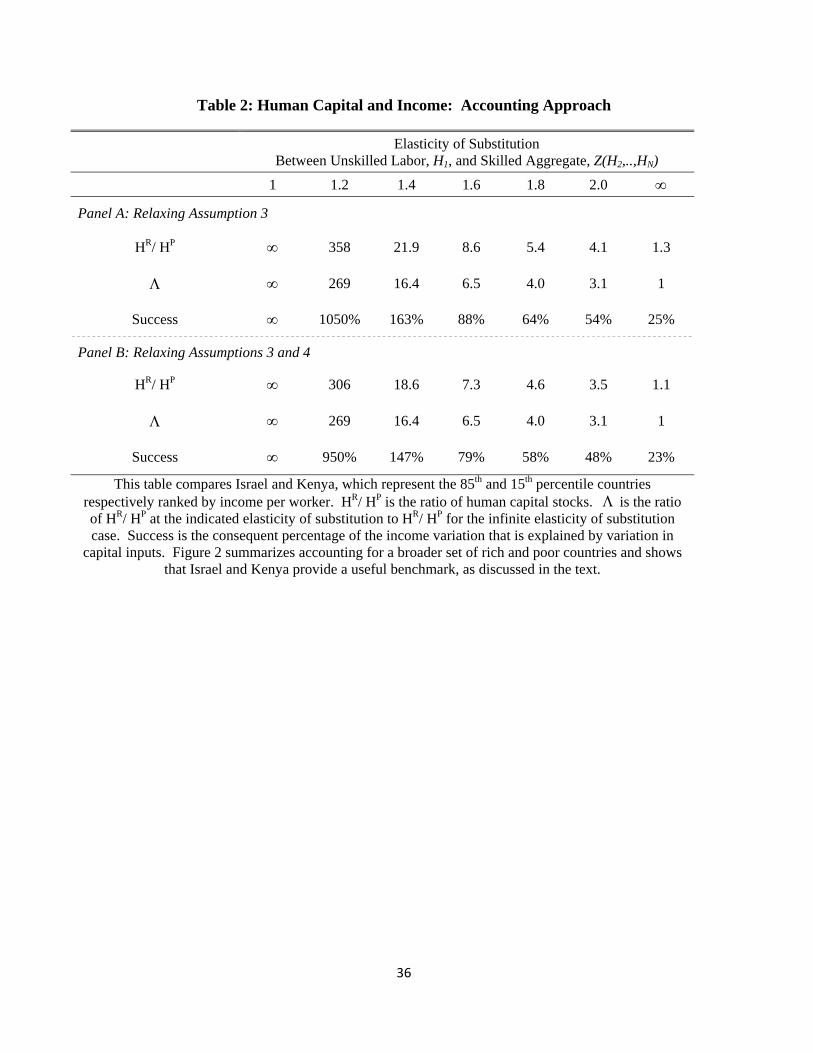
36 

 

Table 2: Human Capital and Income: Accounting Approach

Elasticity of Substitution Between Unskilled Labor, H1, and Skilled Aggregate, Z(H2,..,HN)

1 1.2 1.4 1.6 1.8 2.0

Panel A: Relaxing Assumption 3

HR/ HP 358 21.9 8.6 5.4 4.1 1.3

269 16.4 6.5 4.0 3.1 1

Success 1050% 163% 88% 64% 54% 25%

Panel B: Relaxing Assumptions 3 and 4

HR/ HP 306 18.6 7.3 4.6 3.5 1.1

269 16.4 6.5 4.0 3.1 1

Success 950% 147% 79% 58% 48% 23%

This table compares Israel and Kenya, which represent the 85th and 15th percentile countries respectively ranked by income per worker. HR/ HP is the ratio of human capital stocks. is the ratio of HR/ HP at the indicated elasticity of substitution to HR/ HP for the infinite elasticity of substitution case. Success is the consequent percentage of the income variation that is explained by variation in

capital inputs. Figure 2 summarizes accounting for a broader set of rich and poor countries and shows that Israel and Kenya provide a useful benchmark, as discussed in the text.

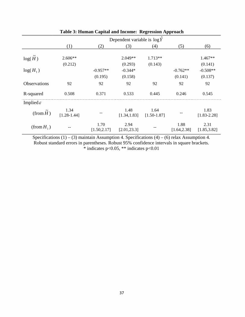
37 

 

Table 3: Human Capital and Income: Regression Approach

Dependent variable is Ylog (1) (2) (3) (4) (5) (6)

log( H~

) 2.606** 2.049** 1.713** 1.467**

(0.212) (0.293) (0.143) (0.141)

log( 1H ) -0.957** -0.344* -0.762** -0.508**

(0.195) (0.158) (0.141) (0.137)

Observations 92 92 92 92 92 92

R-squared 0.508 0.371 0.533 0.445 0.246 0.545

Implied

(from H~

) 1.34

[1.28-1.44] --

1.48 [1.34,1.83]

1.64 [1.50-1.87]

-- 1.83

[1.83-2.28]

(from 1H ) -- 1.70

[1.50,2.17] 2.94

[2.01,23.3] --

1.88 [1.64,2.38]

2.31 [1.85,3.82]

Specifications (1) – (3) maintain Assumption 4. Specifications (4) – (6) relax Assumption 4. Robust standard errors in parentheses. Robust 95% confidence intervals in square brackets.

* indicates p<0.05, ** indicates p<0.01

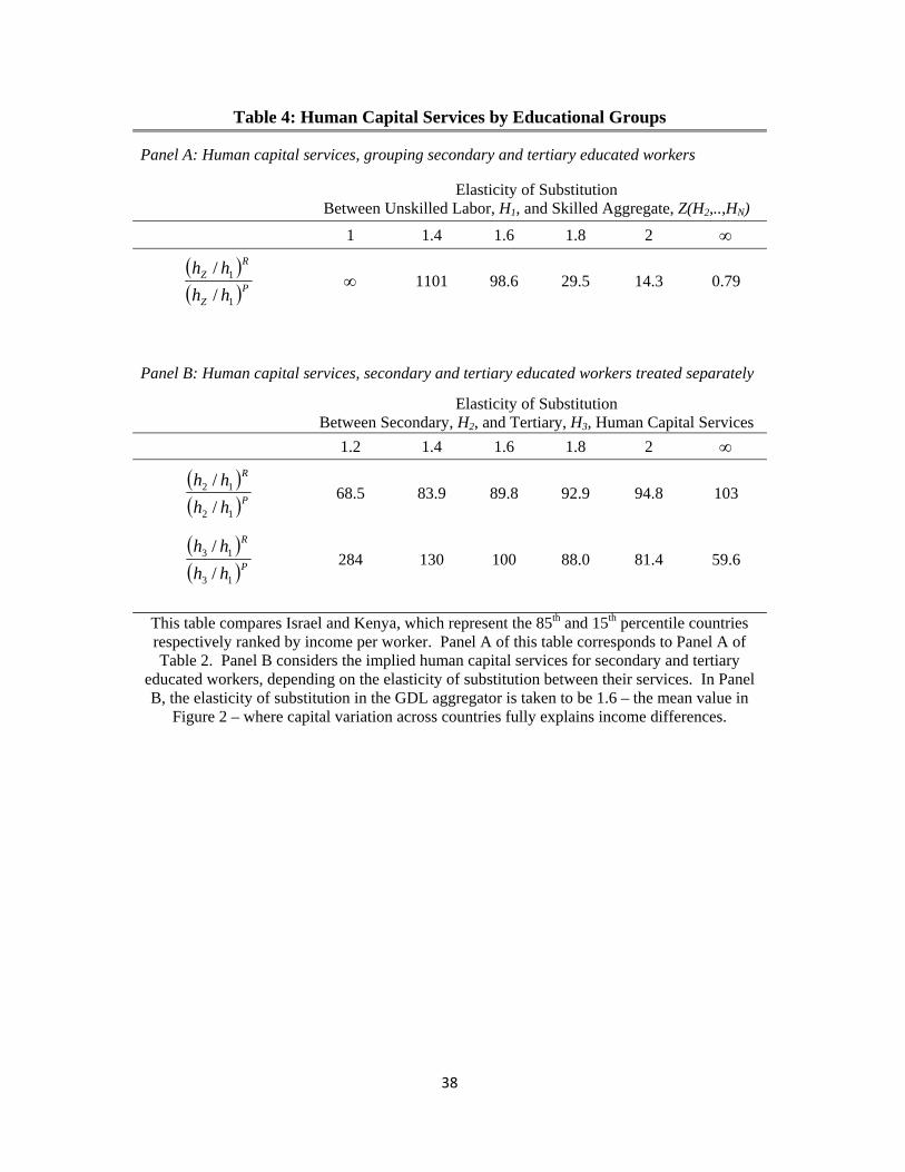
38 

 

Table 4: Human Capital Services by Educational Groups

Panel A: Human capital services, grouping secondary and tertiary educated workers

Elasticity of Substitution Between Unskilled Labor, H1, and Skilled Aggregate, Z(H2,..,HN)

1 1.4 1.6 1.8 2

P

Z

RZ

hh

hh

1

1

/

/ 1101 98.6 29.5 14.3 0.79

Panel B: Human capital services, secondary and tertiary educated workers treated separately

Elasticity of Substitution

Between Secondary, H2, and Tertiary, H3, Human Capital Services

1.2 1.4 1.6 1.8 2

P

R

hh

hh

12

12

/

/ 68.5 83.9 89.8 92.9 94.8 103

P

R

hh

hh

13

13

/

/ 284 130 100 88.0 81.4 59.6

This table compares Israel and Kenya, which represent the 85th and 15th percentile countries respectively ranked by income per worker. Panel A of this table corresponds to Panel A of Table 2. Panel B considers the implied human capital services for secondary and tertiary

educated workers, depending on the elasticity of substitution between their services. In Panel B, the elasticity of substitution in the GDL aggregator is taken to be 1.6 – the mean value in

Figure 2 – where capital variation across countries fully explains income differences.  

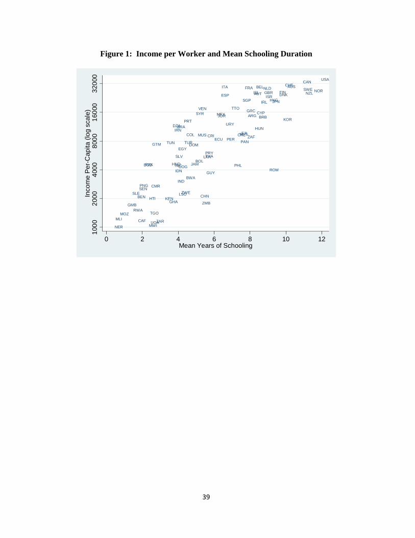
39 

 

Figure 1: Income per Worker and Mean Schooling Duration

ARG

AUS

AUT

BEL

BEN

BGDBOL

BRA

BRB

BWA

CAF

CANCHE

CHL

CHN

CMR

COG

COL CRI

CYP

DNK

DOM

DZA

ECU

EGY

ESPFIN

FJI

FRAGBR

GHAGMB

GRC

GTM

GUY

HKG

HND

HTI

HUN

IDN

IND

IRL

IRN

ISLISR

ITA

JAM

JOR

JPN

KEN

KOR

LKA

LSO

MEX

MLIMOZ

MUS

MWI

MYS

NER

NIC

NLDNOR

NZL

PAK

PANPER

PHL

PNG

PRT

PRY

ROM

RWA

SEN

SGP

SLE

SLV

SWE

SYR

TGO

THA

TTO

TUN TUR

UGA

URY

USA

VEN

ZAF

ZAR

ZMB

ZWE

100

02

000

400

08

000

160

003

2000

Inco

me

Per

-Cap

ita (

log

scal

e)

0 2 4 6 8 10 12Mean Years of Schooling

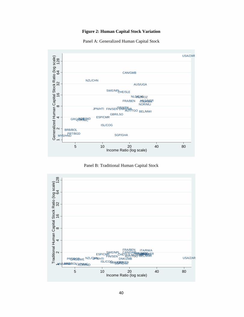
40 

 

Figure 2: Human Capital Stock Variation

Panel A: Generalized Human Capital Stock

USA/ZAR

HKG/NERITA/RWA

BEL/MWI

NOR/MLI

IRL/MOZ

AUS/UGA

NLD/CAF

AUT/TGO

CAN/GMB

FRA/BEN

DNK/ZMB

CHE/SLE

ISR/KEN

SGP/GHA

GBR/LSO

SWE/NPL

FIN/SEN

ISL/COG

ESP/CMR

JPN/HTI

NZL/CHN

KOR/INDCYP/NICGRC/ZWE

PRT/BGDBRB/BOL

MYS/HND

12

48

16

32

64

128

Gen

era

lized

Hum

an

Ca

pita

l Sto

ck R

atio

(lo

g s

cale

)

5 10 20 40 80Income Ratio (log scale)

Panel B: Traditional Human Capital Stock

USA/ZAR

HKG/NERITA/RWA

BEL/MWINOR/MLIIRL/MOZAUS/UGANLD/CAFAUT/TGOCAN/GMBFRA/BEN

DNK/ZMB

CHE/SLE

ISR/KENSGP/GHAGBR/LSO

SWE/NPLFIN/SEN

ISL/COG

ESP/CMR

JPN/HTINZL/CHN

KOR/INDCYP/NIC

GRC/ZWEPRT/BGD

BRB/BOLMYS/HND12

48

16

32

64

128

Tra

diti

ona

l Hu

man

Cap

ital S

tock

Ra

tio (

log

scal

e)

5 10 20 40 80Income Ratio (log scale)

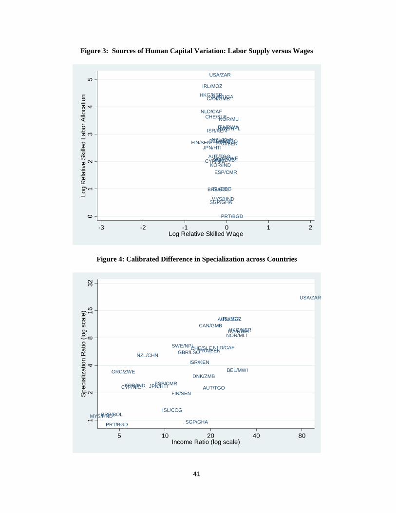
41 

 

Figure 3: Sources of Human Capital Variation: Labor Supply versus Wages

USA/ZAR

HKG/NER

ITA/RWA

BEL/MWI

NOR/MLI

IRL/MOZ

AUS/UGA

NLD/CAF

AUT/TGO

CAN/GMB

FRA/BEN

DNK/ZMB

CHE/SLE

ISR/KEN

SGP/GHA

GBR/LSO

SWE/NPL

FIN/SEN

ISL/COG

ESP/CMR

JPN/HTI

NZL/CHN

KOR/INDCYP/NICGRC/ZWE

PRT/BGD

BRB/BOL

MYS/HND

01

23

45

Log

Re

lativ

e S

kille

d La

bor

Allo

catio

n

-3 -2 -1 0 1 2Log Relative Skilled Wage

Figure 4: Calibrated Difference in Specialization across Countries

USA/ZAR

HKG/NERITA/RWA

BEL/MWI

NOR/MLI

IRL/MOZAUS/UGA

NLD/CAF

AUT/TGO

CAN/GMB

FRA/BEN

DNK/ZMB

CHE/SLE

ISR/KEN

SGP/GHA

GBR/LSOSWE/NPL

FIN/SEN

ISL/COG

ESP/CMRJPN/HTI

NZL/CHN

KOR/INDCYP/NIC

GRC/ZWE

PRT/BGD

BRB/BOLMYS/HND

12

48

1632

Spe

cia

lizat

ion

Ra

tio (

log

sca

le)

5 10 20 40 80Income Ratio (log scale)

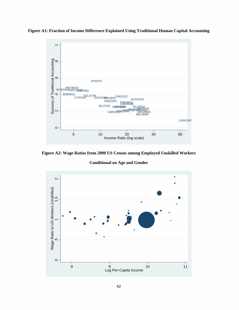
42 

 

Figure A1: Fraction of Income Difference Explained Using Traditional Human Capital Accounting

USA/ZAR

HKG/NERITA/RWA

BEL/MWI

NOR/MLIIRL/MOZ

AUS/UGA

NLD/CAFAUT/TGO

CAN/GMBFRA/BEN

DNK/ZMB

CHE/SLE

ISR/KENSGP/GHA

GBR/LSO

SWE/NPLFIN/SEN

ISL/COG

ESP/CMR

JPN/HTI

NZL/CHN

KOR/IND

CYP/NIC

GRC/ZWEPRT/BGD

BRB/BOL

MYS/HND

0.2

.4.6

.81

Suc

cess

of T

radi

tion

al A

ccou

ntin

g

5 10 20 40 80Income Ratio (log scale)

Figure A2: Wage Ratios from 2000 US Census among Employed Unskilled Workers

Conditional on Age and Gender

0.5

11.

52

Wa

ge R

atio

to U

S W

orke

rs (

Uns

kille

d)

8 9 10 11Log Per-Capita Income