the high-order symplectic finite-difference time-domain … high-order... · the high-order...
TRANSCRIPT

The High-Order Symplectic Finite-Difference Time-Domain Scheme 47
The High-Order Symplectic Finite-Difference Time-Domain Scheme
Wei E.I. Shaa, Xian-liang Wub, Zhi-xiang Huangb and Ming-sheng Chenc
X
The High-Order Symplectic Finite-Difference Time-Domain Scheme
Wei E.I. Shaa, Xian-liang Wub, Zhi-xiang Huangb, and Ming-sheng Chenc a. Department of Electrical and Electronic Engineering, The University of Hong Kong,
Pokfulam Road, Hong Kong, China Email: [email protected]
b. Key Laboratory of Intelligent Computing & Signal Processing, Anhui University, Feixi Road 3, Hefei 230039, China
c. Department of Physics and Electronic Engineering, Hefei Teachers College, Jinzhai Road 327, Hefei 230061, China
Abstract The book chapter will aim at introducing the background knowledge, basic theories, supporting techniques, numerical results, and future research for the high-order symplectic finite-difference time-domain scheme. The theories of symplectic geometry and Hamiltonian are reviewed in Section 2 followed by the symplectiness of Maxwell’s equations presented in Section 3. Next, the numerical stability and dispersion analyses are given in Section 4. Then, in Section 5, we will make a tour of the supporting techniques but do not discuss them in detail. These techniques involve source excitation, perfectly matched layer, near-to-far-field transformation, inhomogeneous boundary treatments, and parameter extractions. The numerical results on propagation, scattering, and guided-wave problems are shown in Section 6. The high-order symplectic finite-difference time-domain scheme demonstrates the powerful advantages and potentials for the time-domain solution of Maxwell’s equations, especially for electrically-large objects and for long-term simulation. Finally, the conclusion and future research are summarized in Section 7. Keywords: Symplectic Finite-Difference Time-Domain Scheme; High-Order Techniques; Symplectic Geometry and Hamiltonian; Numerical Stability and Dispersion; Maxwell’s Equations.
1. Introduction
The traditional finite-difference time-domain (FDTD) method [1-4] , which is explicit second-order-accurate in both space and time, has been widely applied to electromagnetic computation and simulation. The main advantages of the FDTD-based techniques for solving electromagnetic problems are computational simplicity and low operation count. Furthermore, it is well suited to analyze transient problems and is good at modeling
3
Wei E.I. Sha, Xianliang Wu, Zhixiang Huang, and Mingsheng Chen, The High-Order Symplectic Finite-Difference Time-Domain Scheme, Passive Microwave Components and Antennas, Vitaliy Zhurbenko (Ed.), ISBN: 978-953-307-083-4, INTECH, 2010.

Passive Microwave Components and Antennas48
inhomogeneous geometries. Most important of all, the method can readily be implemented on the massive computers. However, the FDTD method has two primary drawbacks, one is the inability to accurately model the curved complex surfaces and material discontinuities by using the staircasing approach with structured grids, and another is the significant accumulated errors from numerical instability, dispersion and anisotropy. Hence fine grids are required to obtain satisfying numerical results, which leads to vast memory requirements and high computational costs, especially for electrically-large domains and for long-term simulation. For the first pitfall, a variety of alternative methods in conjugation with unstructured grids were proposed to reduce the inaccuracy owing to the staircase approximation, including the finite-volume time-domain (FVTD) [5], finite-element time-domain (FETD) [6], and discontinuous Galerkin time-domain (DGTD) methods [7]. Although the methods are easy to treat boundaries, they are less efficient than the traditional FDTD method. Meanwhile, for the traditional FDTD method, a variety of conformal [8-11] and subgridding strategies [12] were proposed also. To overcome the second problem, other high-order spatial discretization strategies were developed. The multi-resolution time-domain (MRTD) [13] and pseudo-spectral time-domain (PSTD) [14] methods reduce the spatial sampling rate drastically, but they are difficult to handle the material interface for modeling the three-dimensional complex objects [15, 16]. Another approach is the staggered fourth-order FDTD method [17-21], which retains the simplicity of the original Yee algorithm and can save computational resources with coarse grids compared to the traditional FDTD method. However, the approach must set lower Courant-Friedrichs-Levy (CFL) number to comply with the stability criterion. Furthermore, the high-order compact difference [22, 23] is easier to treat the inhomogeneous boundaries, but it requires the sparse matrix inversion for each time step. Except for the solvers in space direction, novel solvers in time direction were proposed as well. The Runge-Kutta (R-K) method used in [3, 22] can achieve the high-order accuracy. However, it will consume additional memory and has amplitude error. The alternative direction implicit time-stepping strategy [24-26] is unconditionally stable, but it suffers from the intolerable numerical dispersion once the CFL number is too large. Moreover, the strategy will consume more CPU times caused by the sparse matrix inversion. For the time direction, does a high-order-accurate and energy-conserving solver with low computational costs exist? Surprisingly, Yes! Most physical and chemical phenomenons can be modeled by Hamiltonian differential equations whose time evolution is symplectic transform and flow conserves the symplectic structure [27-29]. The symplectic schemes include a variety of different temporal discretization strategies designed to preserve the global symplectic structure of the phase space for a Hamiltonian system. They have demonstrated their advantages in numerical computation for the Hamiltonian system, especially for long-term simulation. Since Maxwell’s equations can be written as an infinite-dimensional Hamiltonian system, a stable and accurate solution can be obtained by using the symplectic schemes, which preserve the energy of the Hamiltonian system constant. The symplectic schemes can be explicit or implicit and can be generalized to high-order with controllable computational complexity. Recently, researchers from computational electromagnetics society have focused on the symplectic schemes for solving Maxwell’s equations. Symplectic finite-difference time-domain (SFDTD) scheme [30-41], symplectic discrete singular convolution method [42],
symplectic pseudo-spectral time-domain approach [43], symplectic wave equation strategy [44], and multi-symplectic method [45, 46] were proposed and studied. This chapter we will focus on the explicit high-order symplectic integration schemes with the high-order staggered spatial differences for solving the Maxwell’s equations.
2. Mathematical foundations
The partial mathematical proofs are cited from [28, 29, 47].
Definition 1.1. For nnn Rqp 202
02 , , real-symplectic inner product can be defined as
TqJpqp )(),( 0000 (1)
where T denotes transpose and nnnnnxn
nxnnn
II
J22
}0{}0{
which satisfies skew-
symmetric and orthogonal properties, i.e. TJJ , JJJ T 1 . The real-symplectic inner product has the following properties: (1) Bilinear property:
),(),(),(),(),( 000000000000 sqrqsprpsrqp ,
),(),( 0000 qpqp , nRsr 200 , , and R, ;
(2) Skew-symmetric property: ),(),( 0000 pqqp ;
(3) Non-degenerate property: 00 q , 0p , 0),( 00 qp 00 p .
Definition 1.2. If V is a vector space defined on nR2 and the mapping RVV : is
real-symplectic, ),( V is called real-symplectic space and is called real-symplectic structure. Definition 1.3. A linear transform VVT : is called real-symplectic transform, if it
meets ),(),( 0000 qpTqTp , nRqp 200 , .
Definition 1.4. The matrix T is called real-symplectic matrix if JJTT T and
),(),( 0000 qpTqTp . The group including all the real-symplectic matrices is
called real-symplectic group. We sign it as ),2( RnSp .
Definition 1.5. B is an infinitesimally real-symplectic matrix if 0 JBJBT . The infinitesimally real-symplectic matrices can be composed of Lie algebra via anti-commutable Lie Poisson bracket BAABBA ],[ .
Theory 1. B is an infinitesimally real-symplectic matrix ),2()exp( RnSpB . Above mentioned definitions and theory can be extended to complex space.
Definition 2.1. For nnn Cqp 202
02 , , complex-symplectic inner product can be defined as
HqJpqp )(),( 0000 (2)

The High-Order Symplectic Finite-Difference Time-Domain Scheme 49
inhomogeneous geometries. Most important of all, the method can readily be implemented on the massive computers. However, the FDTD method has two primary drawbacks, one is the inability to accurately model the curved complex surfaces and material discontinuities by using the staircasing approach with structured grids, and another is the significant accumulated errors from numerical instability, dispersion and anisotropy. Hence fine grids are required to obtain satisfying numerical results, which leads to vast memory requirements and high computational costs, especially for electrically-large domains and for long-term simulation. For the first pitfall, a variety of alternative methods in conjugation with unstructured grids were proposed to reduce the inaccuracy owing to the staircase approximation, including the finite-volume time-domain (FVTD) [5], finite-element time-domain (FETD) [6], and discontinuous Galerkin time-domain (DGTD) methods [7]. Although the methods are easy to treat boundaries, they are less efficient than the traditional FDTD method. Meanwhile, for the traditional FDTD method, a variety of conformal [8-11] and subgridding strategies [12] were proposed also. To overcome the second problem, other high-order spatial discretization strategies were developed. The multi-resolution time-domain (MRTD) [13] and pseudo-spectral time-domain (PSTD) [14] methods reduce the spatial sampling rate drastically, but they are difficult to handle the material interface for modeling the three-dimensional complex objects [15, 16]. Another approach is the staggered fourth-order FDTD method [17-21], which retains the simplicity of the original Yee algorithm and can save computational resources with coarse grids compared to the traditional FDTD method. However, the approach must set lower Courant-Friedrichs-Levy (CFL) number to comply with the stability criterion. Furthermore, the high-order compact difference [22, 23] is easier to treat the inhomogeneous boundaries, but it requires the sparse matrix inversion for each time step. Except for the solvers in space direction, novel solvers in time direction were proposed as well. The Runge-Kutta (R-K) method used in [3, 22] can achieve the high-order accuracy. However, it will consume additional memory and has amplitude error. The alternative direction implicit time-stepping strategy [24-26] is unconditionally stable, but it suffers from the intolerable numerical dispersion once the CFL number is too large. Moreover, the strategy will consume more CPU times caused by the sparse matrix inversion. For the time direction, does a high-order-accurate and energy-conserving solver with low computational costs exist? Surprisingly, Yes! Most physical and chemical phenomenons can be modeled by Hamiltonian differential equations whose time evolution is symplectic transform and flow conserves the symplectic structure [27-29]. The symplectic schemes include a variety of different temporal discretization strategies designed to preserve the global symplectic structure of the phase space for a Hamiltonian system. They have demonstrated their advantages in numerical computation for the Hamiltonian system, especially for long-term simulation. Since Maxwell’s equations can be written as an infinite-dimensional Hamiltonian system, a stable and accurate solution can be obtained by using the symplectic schemes, which preserve the energy of the Hamiltonian system constant. The symplectic schemes can be explicit or implicit and can be generalized to high-order with controllable computational complexity. Recently, researchers from computational electromagnetics society have focused on the symplectic schemes for solving Maxwell’s equations. Symplectic finite-difference time-domain (SFDTD) scheme [30-41], symplectic discrete singular convolution method [42],
symplectic pseudo-spectral time-domain approach [43], symplectic wave equation strategy [44], and multi-symplectic method [45, 46] were proposed and studied. This chapter we will focus on the explicit high-order symplectic integration schemes with the high-order staggered spatial differences for solving the Maxwell’s equations.
2. Mathematical foundations
The partial mathematical proofs are cited from [28, 29, 47].
Definition 1.1. For nnn Rqp 202
02 , , real-symplectic inner product can be defined as
TqJpqp )(),( 0000 (1)
where T denotes transpose and nnnnnxn
nxnnn
II
J22
}0{}0{
which satisfies skew-
symmetric and orthogonal properties, i.e. TJJ , JJJ T 1 . The real-symplectic inner product has the following properties: (1) Bilinear property:
),(),(),(),(),( 000000000000 sqrqsprpsrqp ,
),(),( 0000 qpqp , nRsr 200 , , and R, ;
(2) Skew-symmetric property: ),(),( 0000 pqqp ;
(3) Non-degenerate property: 00 q , 0p , 0),( 00 qp 00 p .
Definition 1.2. If V is a vector space defined on nR2 and the mapping RVV : is
real-symplectic, ),( V is called real-symplectic space and is called real-symplectic structure. Definition 1.3. A linear transform VVT : is called real-symplectic transform, if it
meets ),(),( 0000 qpTqTp , nRqp 200 , .
Definition 1.4. The matrix T is called real-symplectic matrix if JJTT T and
),(),( 0000 qpTqTp . The group including all the real-symplectic matrices is
called real-symplectic group. We sign it as ),2( RnSp .
Definition 1.5. B is an infinitesimally real-symplectic matrix if 0 JBJBT . The infinitesimally real-symplectic matrices can be composed of Lie algebra via anti-commutable Lie Poisson bracket BAABBA ],[ .
Theory 1. B is an infinitesimally real-symplectic matrix ),2()exp( RnSpB . Above mentioned definitions and theory can be extended to complex space.
Definition 2.1. For nnn Cqp 202
02 , , complex-symplectic inner product can be defined as
HqJpqp )(),( 0000 (2)

Passive Microwave Components and Antennas50
where H denotes complex conjugate transpose or adjoint. The complex-symplectic inner product has the following properties: (1) Conjugate bilinear property:
),(),(),(),(),( 000000000000 sqrqsprpsrqp ,
),(),( 00__
00 qpqp , nCsr 200 , , C, , and
__ is the conjugate
complex of ;
(2) Skew-Hermitian property: ____________0000 ),(),( pqqp ;
(3) Non-degenerate property: 00 q , 0p , 0),( 00 qp 00 p .
Definition 2.2. If V is a vector space defined on nC2 and the mapping CVV :
is complex-symplectic, ),( V is called complex-symplectic space and is called complex-symplectic structure. Definition 2.3. A linear transform VVT : is called complex-symplectic transform, if it
meets ),(),( 0000 qpTqTp , nCqp 200 , .
Definition 2.4. The matrix T is called complex-symplectic matrix if JJTT H and
),(),( 0000 qpTqTp . The group including all the complex-symplectic matrices is
called complex-symplectic group. We sign it as ),2( CnSp .
Definition 2.5. B is an infinitesimally complex-symplectic matrix if 0 JBJBH . The infinitesimally complex-symplectic matrices can be composed of Lie algebra via anti-commutable Lie Poisson bracket BAABBA ],[ .
Theory 2. B is an infinitesimally complex-symplectic matrix ),2()exp( CnSpB .
Definition 3. If ),,( 210
npppp , ),,( 210
nqqqq , nRqp 200 ),( ,
and It 0 , the Hamiltonian canonical equations can be written as
i
i
qH
dtdp
0
,i
i
pH
dtdq
0
, ni ,2,1 (3)
where ),,( 000 tqpH is the Hamiltonian function, is the phase space, and I is
the extended phase space.
Theory 3. If the solution of (3) at any time t is ),( qp and ),( qp still satisfies the
equation (3), the Jacobi matrix is a symplectic matrix
JJT (4)
where
00
00
00 ////
),(),(
qqpqqppp
qpqp
.
Theory 4. If the time evolution operator of (3) from 0t to t is ),( 0tt and
),)(,(),( 000 qpttqp
, the operator conserves the symplectic structure 0
0 ),( tt (5)
where dqdp ^ , 000 ^ dqdp , and ),( 0tt is the conjugate operator of
),( 0tt . The time evolution operator is also called Hamiltonian flow or symplectic flow.
Theory 5. The matrix
0
0A
AL
)cos()sin()sin()cos(
)exp(AAAA
L .
Theory 6. If the matrix
0
0A
AL and TAA , we have: (1) L is skew-symmetric,
i.e. TLL ; (2) )exp(L are both orthogonal and real-symplectic matrices. We call
)exp(L symplectic-orthogonal matrix.
Theory 7. If the matrix
0
0A
AL and HAA , we have: (1) L is skew-Hermitian,
i.e. HLL ; (2) )exp(L are both unitary and complex-symplectic matrices. We call
)exp(L symplectic-unitary matrix.
3. Symplectic framework of Maxwell’s equations
A Helicity generating function [48] for Maxwell’s equations in free space is introduced as
)11(21)(
00
EEHHEH,
G (6)
where Tzyx EEE ),,(E is the electric field vector, T
zyx HHH ),,(H is the
magnetic field vector, and 0 and 0 are the permittivity and permeability of free space. The differential form of the Hamiltonian is
EH
G
t
, H
EG
t
(7)
According to the variation principle, we can derive Maxwell’s equations of free space from (7)
EH
EH
ˆˆ Lt
(8)

The High-Order Symplectic Finite-Difference Time-Domain Scheme 51
where H denotes complex conjugate transpose or adjoint. The complex-symplectic inner product has the following properties: (1) Conjugate bilinear property:
),(),(),(),(),( 000000000000 sqrqsprpsrqp ,
),(),( 00__
00 qpqp , nCsr 200 , , C, , and
__ is the conjugate
complex of ;
(2) Skew-Hermitian property: ____________0000 ),(),( pqqp ;
(3) Non-degenerate property: 00 q , 0p , 0),( 00 qp 00 p .
Definition 2.2. If V is a vector space defined on nC2 and the mapping CVV :
is complex-symplectic, ),( V is called complex-symplectic space and is called complex-symplectic structure. Definition 2.3. A linear transform VVT : is called complex-symplectic transform, if it
meets ),(),( 0000 qpTqTp , nCqp 200 , .
Definition 2.4. The matrix T is called complex-symplectic matrix if JJTT H and
),(),( 0000 qpTqTp . The group including all the complex-symplectic matrices is
called complex-symplectic group. We sign it as ),2( CnSp .
Definition 2.5. B is an infinitesimally complex-symplectic matrix if 0 JBJBH . The infinitesimally complex-symplectic matrices can be composed of Lie algebra via anti-commutable Lie Poisson bracket BAABBA ],[ .
Theory 2. B is an infinitesimally complex-symplectic matrix ),2()exp( CnSpB .
Definition 3. If ),,( 210
npppp , ),,( 210
nqqqq , nRqp 200 ),( ,
and It 0 , the Hamiltonian canonical equations can be written as
i
i
qH
dtdp
0
,i
i
pH
dtdq
0
, ni ,2,1 (3)
where ),,( 000 tqpH is the Hamiltonian function, is the phase space, and I is
the extended phase space.
Theory 3. If the solution of (3) at any time t is ),( qp and ),( qp still satisfies the
equation (3), the Jacobi matrix is a symplectic matrix
JJT (4)
where
00
00
00 ////
),(),(
qqpqqppp
qpqp
.
Theory 4. If the time evolution operator of (3) from 0t to t is ),( 0tt and
),)(,(),( 000 qpttqp
, the operator conserves the symplectic structure 0
0 ),( tt (5)
where dqdp ^ , 000 ^ dqdp , and ),( 0tt is the conjugate operator of
),( 0tt . The time evolution operator is also called Hamiltonian flow or symplectic flow.
Theory 5. The matrix
0
0A
AL
)cos()sin()sin()cos(
)exp(AAAA
L .
Theory 6. If the matrix
0
0A
AL and TAA , we have: (1) L is skew-symmetric,
i.e. TLL ; (2) )exp(L are both orthogonal and real-symplectic matrices. We call
)exp(L symplectic-orthogonal matrix.
Theory 7. If the matrix
0
0A
AL and HAA , we have: (1) L is skew-Hermitian,
i.e. HLL ; (2) )exp(L are both unitary and complex-symplectic matrices. We call
)exp(L symplectic-unitary matrix.
3. Symplectic framework of Maxwell’s equations
A Helicity generating function [48] for Maxwell’s equations in free space is introduced as
)11(21)(
00
EEHHEH,
G (6)
where Tzyx EEE ),,(E is the electric field vector, T
zyx HHH ),,(H is the
magnetic field vector, and 0 and 0 are the permittivity and permeability of free space. The differential form of the Hamiltonian is
EH
G
t
, H
EG
t
(7)
According to the variation principle, we can derive Maxwell’s equations of free space from (7)
EH
EH
ˆˆ Lt
(8)

Passive Microwave Components and Antennas52
333300
3300
33
}0{1
1}0{
R
RL
, EE
0
0ˆ
(9)
0
0
0
xy
xz
yz
R (10)
where 33}0{ is the 33 null matrix and R is the three-dimensional curl operator. However, the Helicity generating function has little physical meaning. It is known however that the total stored energy of electromagnetic field is constant in an energy conserving system. Hence, the total stored energy is taken to be the Hamiltonian
dVGV
HBDE
21
21
(11)
It is well known that
AH 0
1
(12)
t
AE (13)
where A and are the vector and scalar potentials and can be uniquely defined by using a Lorentz gauge or a Coulomb gauge. If we define the conjugate momentum and coordinate as
)(0 t
AΠ (14)
AQ (15) The Hamiltonian can be rewritten as
dVGV
QQΠΠ
00 21
21
(16)
The equations of motion is to be
tG
Q
Π
, t
G
Π
Q
(17)
If we define / t and 0 0At
(Lorentz gauge), the above is equivalent to
Maxwell’s equations. The time evolution of (8) from 0t to tt can be written as
)0(ˆ)exp()(ˆ
EH
EH
Ltt (18)
where )exp( Lt is the time evolution matrix (TEMA) or symplectic flow of Maxwell’s equations. For infinite-dimensional real space, we define the inner product
rrrrr dtGtFtGtF ),(),(),(),,( (19)
where zy zyx eeer x is the position vector and t is the time variable. According
to the identity both in the generalized distribution space and in the Hilbert space /,,/ GFGF , zyx ,, (20)
we can know / is a skew-symmetric operator. Hence R is a symmetric operator, i.e. TRR . Based on Theory 6, the TEMA of Maxwell’s equations is a symplectic-orthogonal
matrix in real space. For infinite-dimensional complex space, we define the inner product
rrrrr dtGtFtGtF
________
),(),(),(),,( (21)
The forward and inverse Fourier transforms for electromagnetic field components are respectively
rrkrk 00 djtFtF )exp(),(
21),(~ 0
(22)
000 krkkr djtFtF )exp(),(~
21),( 0
(23)
where 0j is the imaginary unit and zzyyx kkk eeek x0 is the wave vector. For
simplicity, we use the shorthand notations FF ~ and FF ~1 . In the beginning, with the help of Parseval theorem
GFGF ~,~, 1 (24)
we know that the Fourier operator is a unitary operator, i.e. H 1 .
Next, using the differential property of Fourier transform zyxFkjF ,,,~0 ,
we can obtain the spectral-domain form of Maxwell’s equations
The High-Order Symplectic Finite-Difference Time-Domain Scheme 53
333300
3300
33
}0{1
1}0{
R
RL
, EE
0
0ˆ
(9)
0
0
0
xy
xz
yz
R (10)
where 33}0{ is the 33 null matrix and R is the three-dimensional curl operator. However, the Helicity generating function has little physical meaning. It is known however that the total stored energy of electromagnetic field is constant in an energy conserving system. Hence, the total stored energy is taken to be the Hamiltonian
dVGV
HBDE
21
21
(11)
It is well known that
AH 0
1
(12)
t
AE (13)
where A and are the vector and scalar potentials and can be uniquely defined by using a Lorentz gauge or a Coulomb gauge. If we define the conjugate momentum and coordinate as
)(0 t
AΠ (14)
AQ (15) The Hamiltonian can be rewritten as
dVGV
QQΠΠ
00 21
21
(16)
The equations of motion is to be
tG
Q
Π
, t
G
Π
Q
(17)
If we define / t and 0 0At
(Lorentz gauge), the above is equivalent to
Maxwell’s equations. The time evolution of (8) from 0t to tt can be written as
)0(ˆ)exp()(ˆ
EH
EH
Ltt (18)
where )exp( Lt is the time evolution matrix (TEMA) or symplectic flow of Maxwell’s equations. For infinite-dimensional real space, we define the inner product
rrrrr dtGtFtGtF ),(),(),(),,( (19)
where zy zyx eeer x is the position vector and t is the time variable. According
to the identity both in the generalized distribution space and in the Hilbert space /,,/ GFGF , zyx ,, (20)
we can know / is a skew-symmetric operator. Hence R is a symmetric operator, i.e. TRR . Based on Theory 6, the TEMA of Maxwell’s equations is a symplectic-orthogonal
matrix in real space. For infinite-dimensional complex space, we define the inner product
rrrrr dtGtFtGtF
________
),(),(),(),,( (21)
The forward and inverse Fourier transforms for electromagnetic field components are respectively
rrkrk 00 djtFtF )exp(),(
21),(~ 0
(22)
000 krkkr djtFtF )exp(),(~
21),( 0
(23)
where 0j is the imaginary unit and zzyyx kkk eeek x0 is the wave vector. For
simplicity, we use the shorthand notations FF ~ and FF ~1 . In the beginning, with the help of Parseval theorem
GFGF ~,~, 1 (24)
we know that the Fourier operator is a unitary operator, i.e. H 1 .
Next, using the differential property of Fourier transform zyxFkjF ,,,~0 ,
we can obtain the spectral-domain form of Maxwell’s equations

Passive Microwave Components and Antennas54
EH
EH ~
~
}0{~1
~1}0{~~
333300
3300
33
R
R
t
(25)
00
0~
00
00
00
33
xy
xz
yz
kjkjkjkjkjkj
R (26)
where R~ is a Hermitian matrix, i.e. RR H ~~ . Finally, considering the unitary property of the Fourier operator, we can convert the spectral-domain form (25) into the spatial-domain form (27)
EH
EH
ˆ}0{~1
~1}0{
ˆ33333333
00
33333300
33
R
R
t H
H
(27)
where 3 3 ( )diag . It is easy to show that 3 3 3 3 3 3HR R is a Hermitian matrix, i.e.
HRR . Based on Theory 7, the TEMA of Maxwell’s equations is a symplectic-unitary matrix in complex space. It is well known that the total energy of electromagnetic field in free space can be represented as
V
V dV20
200 ||
21||
21ˆ,ˆ,
21 EHEEHH (28)
No matter in complex space or in real space, the TEMA )exp( Lt accurately conserves
the total energy of electromagnetic field. In other words, the TEMA )exp( Lt only rotates the electromagnetic field components (Theory 5). In addition, if an algorithm can accurately conserve the total energy of electromagnetic field, it is to be unconditionally stable. Both in complex space and in real space, we can split L into U and V
VUL (29)
3333
3300
33
}0{}0{
1}0{ RU ,
333300
3333
}0{1}0{}0{
RV
(30)
The split TEMA can be approximated by the explicit m-stage pth-order symplectic integration scheme [32, 49]
11
)exp()exp()(exp
pttl
m
ltlt OUcVdVU (31)
where lc and ld are the symplectic integrators and satisfy the time-reversible [49] or symmetric relations [50], i.e.
)1(1 mlcc lml , )11( mldd lml , 0md (32)
)1(1 mlcd lml (33) Table 1 lists the three-order symmetric symplectic integrators and the fourth-order time-reversible symplectic integrators [40]. The time-stepping diagram for the five-stage fourth-order symplectic scheme [32] is shown in Fig. 1.
Table 1. The three-order symmetric symplectic integrators and the fourth-order time-reversible symplectic integrators.
Fig. 1. Time-stepping diagram for the five-stage fourth-order symplectic scheme.
For real space, TRR and therefore U and V are the infinitesimally real-symplectic
matrices. Likewise, for complex space, HRR and therefore U and V are the
infinitesimally complex-symplectic matrices. In particular, we have: (1) U and V can be composed of Lie algebra semicolon at Line 11. (2) )exp( Vd tl and )exp( Uc tl are the symplectic matrices.

The High-Order Symplectic Finite-Difference Time-Domain Scheme 55
EH
EH ~
~
}0{~1
~1}0{~~
333300
3300
33
R
R
t
(25)
00
0~
00
00
00
33
xy
xz
yz
kjkjkjkjkjkj
R (26)
where R~ is a Hermitian matrix, i.e. RR H ~~ . Finally, considering the unitary property of the Fourier operator, we can convert the spectral-domain form (25) into the spatial-domain form (27)
EH
EH
ˆ}0{~1
~1}0{
ˆ33333333
00
33333300
33
R
R
t H
H
(27)
where 3 3 ( )diag . It is easy to show that 3 3 3 3 3 3HR R is a Hermitian matrix, i.e.
HRR . Based on Theory 7, the TEMA of Maxwell’s equations is a symplectic-unitary matrix in complex space. It is well known that the total energy of electromagnetic field in free space can be represented as
V
V dV20
200 ||
21||
21ˆ,ˆ,
21 EHEEHH (28)
No matter in complex space or in real space, the TEMA )exp( Lt accurately conserves
the total energy of electromagnetic field. In other words, the TEMA )exp( Lt only rotates the electromagnetic field components (Theory 5). In addition, if an algorithm can accurately conserve the total energy of electromagnetic field, it is to be unconditionally stable. Both in complex space and in real space, we can split L into U and V
VUL (29)
3333
3300
33
}0{}0{
1}0{ RU ,
333300
3333
}0{1}0{}0{
RV
(30)
The split TEMA can be approximated by the explicit m-stage pth-order symplectic integration scheme [32, 49]
11
)exp()exp()(exp
pttl
m
ltlt OUcVdVU (31)
where lc and ld are the symplectic integrators and satisfy the time-reversible [49] or symmetric relations [50], i.e.
)1(1 mlcc lml , )11( mldd lml , 0md (32)
)1(1 mlcd lml (33) Table 1 lists the three-order symmetric symplectic integrators and the fourth-order time-reversible symplectic integrators [40]. The time-stepping diagram for the five-stage fourth-order symplectic scheme [32] is shown in Fig. 1.
Table 1. The three-order symmetric symplectic integrators and the fourth-order time-reversible symplectic integrators.
Fig. 1. Time-stepping diagram for the five-stage fourth-order symplectic scheme.
For real space, TRR and therefore U and V are the infinitesimally real-symplectic
matrices. Likewise, for complex space, HRR and therefore U and V are the
infinitesimally complex-symplectic matrices. In particular, we have: (1) U and V can be composed of Lie algebra semicolon at Line 11. (2) )exp( Vd tl and )exp( Uc tl are the symplectic matrices.

Passive Microwave Components and Antennas56
Although the orthogonal properties can not be retained by the two matrices )exp( Vd tl
and )exp( Uc tl , the determinants of them are equal to 1 [51]. Thus the explicit symplectic integration scheme is conditionally stable and does not have amplitude error.
4. Numerical stability and dispersion analyses
We first present the numerical stability and dispersion analyses for the one-dimensional problem, then extend them to the three-dimensional problem.
Given the field components ),( nx
ny EHnF at the n-th time step, the field components
),( 11 nx
ny EH1nF at the (n+1)-th time step can be represented as
n1n FF S (34) where S is the amplification matrix. The well-known plane wave expansions are
)(exp),,,( 00 zzyyxx kkkjkijftzyxF (35)
cossin0kkx , sinsin0kk y , cos0kkz (36)
where 0k is the numerical wave number, and and are spherical angles. Using the q-th staggered differences to approximate the spatial first-order derivatives, we get
F
Fkrjkrj
W
rkjiFrkjiFWzF
z
q
r z
zzzzr
q
r zr
2/
1
00
2/
1
)2/1(exp)2/1(exp
)2/1,,()2/1,,(
(37)
where
2/
1
00 )2/1(exp)2/1(expq
r z
zzzzrz
krjkrjW , and rW are
the spatial difference coefficients [40] as shown in Table 2. The continuous Maxwell’s equations
x
y
x
y
EH
z
zEH
t 01
10
(38)
can be semi-discretized as
x
y
z
z
x
y
EH
EH
t 01
10
(39)
If we set
00
10 zU ,
01
00
zV
, and use the symplectic integration
scheme for approximating the TEMA of Maxwell’s equations, the amplification matrix S can be written as
m
l
tlz
tlz
cdS
1 10
111101
(40)
Each stage of (40) is the symplectic transform, and therefore 1)exp(det Uc tl and
1)exp(det Vd tl [51], which can be easily testified by (40). As a result, 1det S . The amplification matrix is
2221
1211
SSSS
S (41)
and its eigenvalues satisfy the following equation
0)( 2112221122112 SSSSSS (42)
Notice that 2211)( SSStr and 1det)( 21122211 SSSSS , (42) can be rewritten as
01)(2 Str (43)
and its solutions2
)(4)( 20
2,1StrjStr
. A stable algorithm requires 1|| 2,1 ,
which says that 2|)(| Str . The right side of (40) is multiplied term by term, then we get
lzt
m
ll vgStr 222
01
2)(
(44)
ll
ll
ll
ll
jimjijiji
jijijimjijiji
jijil cdcdcddcdcdcg
2211
2211
2211
221111
(45)
where 1
0 v is the velocity of light.

The High-Order Symplectic Finite-Difference Time-Domain Scheme 57
Although the orthogonal properties can not be retained by the two matrices )exp( Vd tl
and )exp( Uc tl , the determinants of them are equal to 1 [51]. Thus the explicit symplectic integration scheme is conditionally stable and does not have amplitude error.
4. Numerical stability and dispersion analyses
We first present the numerical stability and dispersion analyses for the one-dimensional problem, then extend them to the three-dimensional problem.
Given the field components ),( nx
ny EHnF at the n-th time step, the field components
),( 11 nx
ny EH1nF at the (n+1)-th time step can be represented as
n1n FF S (34) where S is the amplification matrix. The well-known plane wave expansions are
)(exp),,,( 00 zzyyxx kkkjkijftzyxF (35)
cossin0kkx , sinsin0kk y , cos0kkz (36)
where 0k is the numerical wave number, and and are spherical angles. Using the q-th staggered differences to approximate the spatial first-order derivatives, we get
F
Fkrjkrj
W
rkjiFrkjiFWzF
z
q
r z
zzzzr
q
r zr
2/
1
00
2/
1
)2/1(exp)2/1(exp
)2/1,,()2/1,,(
(37)
where
2/
1
00 )2/1(exp)2/1(expq
r z
zzzzrz
krjkrjW , and rW are
the spatial difference coefficients [40] as shown in Table 2. The continuous Maxwell’s equations
x
y
x
y
EH
z
zEH
t 01
10
(38)
can be semi-discretized as
x
y
z
z
x
y
EH
EH
t 01
10
(39)
If we set
00
10 zU ,
01
00
zV
, and use the symplectic integration
scheme for approximating the TEMA of Maxwell’s equations, the amplification matrix S can be written as
m
l
tlz
tlz
cdS
1 10
111101
(40)
Each stage of (40) is the symplectic transform, and therefore 1)exp(det Uc tl and
1)exp(det Vd tl [51], which can be easily testified by (40). As a result, 1det S . The amplification matrix is
2221
1211
SSSS
S (41)
and its eigenvalues satisfy the following equation
0)( 2112221122112 SSSSSS (42)
Notice that 2211)( SSStr and 1det)( 21122211 SSSSS , (42) can be rewritten as
01)(2 Str (43)
and its solutions2
)(4)( 20
2,1StrjStr
. A stable algorithm requires 1|| 2,1 ,
which says that 2|)(| Str . The right side of (40) is multiplied term by term, then we get
lzt
m
ll vgStr 222
01
2)(
(44)
ll
ll
ll
ll
jimjijiji
jijijimjijiji
jijil cdcdcddcdcdcg
2211
2211
2211
221111
(45)
where 1
0 v is the velocity of light.
Passive Microwave Components and Antennas58
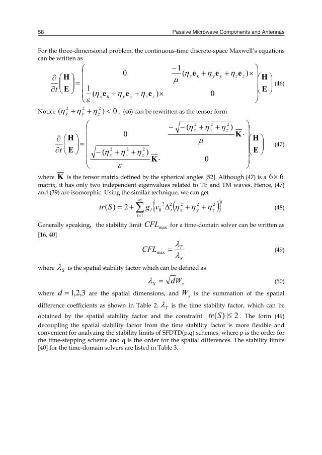
For the three-dimensional problem, the continuous-time discrete-space Maxwell’s equations can be written as
EH
eee
eee
EH
x
x
0)(1
)(10
zzyyx
zzyyx
t
(46)
Notice 0)( 222 zyx , (46) can be rewritten as the tensor form
EH
K
K
EH
0)(
)(0
222
222
zyx
zyx
t (47)
where K is the tensor matrix defined by the spherical angles [52]. Although (47) is a 66 matrix, it has only two independent eigenvalues related to TE and TM waves. Hence, (47) and (39) are isomorphic. Using the similar technique, we can get
lzyxt
m
ll vgStr 22222
01
2)(
(48)
Generally speaking,the stability limit maxCFL for a time-domain solver can be written as [16, 40]
S
TCFL
max (49)
where S is the spatial stability factor which can be defined as
sS Wd (50)
where 3,2,1d are the spatial dimensions, and sW is the summation of the spatial
difference coefficients as shown in Table 2. T is the time stability factor, which can be
obtained by the spatial stability factor and the constraint 2|)(| Str . The form (49) decoupling the spatial stability factor from the time stability factor is more flexible and convenient for analyzing the stability limits of SFDTD(p,q) schemes, where p is the order for the time-stepping scheme and q is the order for the spatial differences. The stability limits [40] for the time-domain solvers are listed in Table 3.
Order (q) 1W 2W 3W 4W SW
2 1 2 4 9/8 -1/24 7/3 6 75/64 -25/384 3/640 149/60
8 1225/1024 -245/3072 49/5120 -5/7168 2161/840
Table. 2. The spatial difference coefficients.
Algorithms CFL number
FDTD(2,2) 0.577
FDTD(2,4) 0.495 J-Fang(4,4) 0.577
R-K(4,4) 0.700 SFDTD(4,4) 0.858
Table. 3. The stability limits for different algorithms.
The disperision relation can be written as 2/)(arccos Strt (51)
and the phase velocity error can be defined as
0
010log20
vvv
Err p (52)
where 0k
vp
is the numerical phase velocity. The phase velocity error as a function of
points per wavelength (PPW) is shown in Fig. 2. The SFDTD(4,4) scheme is superior to the traditional FDTD(2,2) method, FDTD(2,4) approach [18], and R-K(4,4) [3] strategy. Although the J-Fang(4,4) method [17] is the best solver, but it suffers from the intractable boundary treatments.

The High-Order Symplectic Finite-Difference Time-Domain Scheme 59
For the three-dimensional problem, the continuous-time discrete-space Maxwell’s equations can be written as
EH
eee
eee
EH
x
x
0)(1
)(10
zzyyx
zzyyx
t
(46)
Notice 0)( 222 zyx , (46) can be rewritten as the tensor form
EH
K
K
EH
0)(
)(0
222
222
zyx
zyx
t (47)
where K is the tensor matrix defined by the spherical angles [52]. Although (47) is a 66 matrix, it has only two independent eigenvalues related to TE and TM waves. Hence, (47) and (39) are isomorphic. Using the similar technique, we can get
lzyxt
m
ll vgStr 22222
01
2)(
(48)
Generally speaking,the stability limit maxCFL for a time-domain solver can be written as [16, 40]
S
TCFL
max (49)
where S is the spatial stability factor which can be defined as
sS Wd (50)
where 3,2,1d are the spatial dimensions, and sW is the summation of the spatial
difference coefficients as shown in Table 2. T is the time stability factor, which can be
obtained by the spatial stability factor and the constraint 2|)(| Str . The form (49) decoupling the spatial stability factor from the time stability factor is more flexible and convenient for analyzing the stability limits of SFDTD(p,q) schemes, where p is the order for the time-stepping scheme and q is the order for the spatial differences. The stability limits [40] for the time-domain solvers are listed in Table 3.
Order (q) 1W 2W 3W 4W SW
2 1 2 4 9/8 -1/24 7/3 6 75/64 -25/384 3/640 149/60
8 1225/1024 -245/3072 49/5120 -5/7168 2161/840
Table. 2. The spatial difference coefficients.
Algorithms CFL number
FDTD(2,2) 0.577
FDTD(2,4) 0.495 J-Fang(4,4) 0.577
R-K(4,4) 0.700 SFDTD(4,4) 0.858
Table. 3. The stability limits for different algorithms.
The disperision relation can be written as 2/)(arccos Strt (51)
and the phase velocity error can be defined as
0
010log20
vvv
Err p (52)
where 0k
vp
is the numerical phase velocity. The phase velocity error as a function of
points per wavelength (PPW) is shown in Fig. 2. The SFDTD(4,4) scheme is superior to the traditional FDTD(2,2) method, FDTD(2,4) approach [18], and R-K(4,4) [3] strategy. Although the J-Fang(4,4) method [17] is the best solver, but it suffers from the intractable boundary treatments.

Passive Microwave Components and Antennas60
6 7 8 9 10 11 12 13−90
−80
−70
−60
−50
−40
−30
PPW
Rel
ativ
e P
hase
Vel
ocity
Err
or (d
B)
SFDTD(4,4)FDTD(2,4)FDTD(2,2)
(a) CFL=0.4
6 7 8 9 10 11 12 13−95
−90
−85
−80
−75
−70
−65
−60
−55
PPW
Rel
ativ
e P
hase
Vel
ocity
Err
or (d
B)
SFDTD(4,4)R−K(4,4)J−Fang(4,4)
(b) CFL=0.5
Fig. 2. Numerical dispersion comparisons. Dispersion curves for a plane wave traveling at 60 and 30 .
5. Supporting techniques The basic formulations of the high-order SFDTD scheme are presented in [32, 38]. The perfectly matched layer (PML) absorbing boundary conditions are given in [31, 41-43]. The total field and scattered field techniques are developed in [34, 53]. The near-to-far-field transformation is put forward in [38]. The high-order subcell and the high-order conformal strategies are proposed in [38, 39, 54, 55, 56]. The parameter extraction and source excitation techniques are discussed in [41]. A function of space and time evaluated at a discrete point in the Cartesian lattice and at a discrete stage in the time step can be notated as
))(,,,(),,,( /tlzyx
mln nkjiFtzyxF (53)
where x , y , and z are, respectively, the lattice space increments in the x , y , and z
coordinate directions, t is the time increment, i , j , k , ,n l , and m are integers,
mln / denotes the thl stage after n time steps, m is the total stage number, and
l is the fixed time with respect to the thl stage. Take the SFDTD(p,4) scheme for example, the update equation for the scaled electric field component is given by
23,,
21
23,,
21
,23,
21,
23,
21
21,,
21
21,,
21
,21,
21,
21,
21
,,211,,
21ˆ,,
21ˆ
//2
//2
//1
//1
/)1(/
kjiHkjiH
kjiHkjiH
kjiHkjiH
kjiHkjiH
kjikjiEkjiE
mlny
mlnyz
mlnz
mlnzy
mlny
mlnyz
mlnz
mlnzy
r
mlnx
mlnx
(54)
yly CFLd 89
1 zlz CFLd 89
1 (55)
yly CFLd
241
2 zlz CFLd
241
2 (56)
y
tyCFL
00
1
z
tzCFL
00
1
(57)

The High-Order Symplectic Finite-Difference Time-Domain Scheme 61
6 7 8 9 10 11 12 13−90
−80
−70
−60
−50
−40
−30
PPW
Rel
ativ
e P
hase
Vel
ocity
Err
or (d
B)
SFDTD(4,4)FDTD(2,4)FDTD(2,2)
(a) CFL=0.4
6 7 8 9 10 11 12 13−95
−90
−85
−80
−75
−70
−65
−60
−55
PPW
Rel
ativ
e P
hase
Vel
ocity
Err
or (d
B)
SFDTD(4,4)R−K(4,4)J−Fang(4,4)
(b) CFL=0.5
Fig. 2. Numerical dispersion comparisons. Dispersion curves for a plane wave traveling at 60 and 30 .
5. Supporting techniques The basic formulations of the high-order SFDTD scheme are presented in [32, 38]. The perfectly matched layer (PML) absorbing boundary conditions are given in [31, 41-43]. The total field and scattered field techniques are developed in [34, 53]. The near-to-far-field transformation is put forward in [38]. The high-order subcell and the high-order conformal strategies are proposed in [38, 39, 54, 55, 56]. The parameter extraction and source excitation techniques are discussed in [41]. A function of space and time evaluated at a discrete point in the Cartesian lattice and at a discrete stage in the time step can be notated as
))(,,,(),,,( /tlzyx
mln nkjiFtzyxF (53)
where x , y , and z are, respectively, the lattice space increments in the x , y , and z
coordinate directions, t is the time increment, i , j , k , ,n l , and m are integers,
mln / denotes the thl stage after n time steps, m is the total stage number, and
l is the fixed time with respect to the thl stage. Take the SFDTD(p,4) scheme for example, the update equation for the scaled electric field component is given by
23,,
21
23,,
21
,23,
21,
23,
21
21,,
21
21,,
21
,21,
21,
21,
21
,,211,,
21ˆ,,
21ˆ
//2
//2
//1
//1
/)1(/
kjiHkjiH
kjiHkjiH
kjiHkjiH
kjiHkjiH
kjikjiEkjiE
mlny
mlnyz
mlnz
mlnzy
mlny
mlnyz
mlnz
mlnzy
r
mlnx
mlnx
(54)
yly CFLd 89
1 zlz CFLd 89
1 (55)
yly CFLd
241
2 zlz CFLd
241
2 (56)
y
tyCFL
00
1
z
tzCFL
00
1
(57)

Passive Microwave Components and Antennas62
where r is the relative permittivity. For the cubic grid, zyx and
CFLCFLCFLCFL zyx .
The source conditions for xE field at the plane 2kk are given as follows
211,,
21ˆ1,,
21ˆ
2/
,22/
2/ kHkjiEkjiE mln
incyzmln
xmln
x (58)
23
21,,
21ˆ,,
21ˆ
2/
,2
2/
,12/
2/
kH
kHkjiEkjiE
mlnincyz
mlnincyz
mlnx
mlnx
(59)
211,,
21ˆ1,,
21ˆ
2/
,22/
2/ kHkjiEkjiE mln
incyzmln
xmln
x (60)
where incyH , is the one-dimensional incident wave source.
The discretized y subcomponent of xE field in the PML region can be deduced as
kjiHkjiH
kjiHkjiH
kjiEkjiE
mlnz
mlnzy
mlnz
mlnzy
mlnxy
mlnxy
,23,
21,
23,
21
,21,
21,
21,
21
)exp(1,,21ˆ)exp(,,
21ˆ
//2
//1
/)1(/
(61)
0
,,21
kjid ytl
(62)
where y is the local electric conductivity at
kji ,,
21
in the PML region. Polynomial
conductivities are employed varying from zeros at the vacuum-layer interface to max,y at
the outer side of the PML layer, i.e.
max,)( yy (63)
where is the layer thickness, is the distance from the interface, and is the polynomial order. When 3 , max,y can be set as
ybr
br
y
08.0max, (64)
where br and b
r are the permittivity and permeability of the background media. For the free space, 1b b
r r .Considering the electric and magnetic fields are interleaved in the space lattice at intervals of half space increments, we must use efficient interpolation method to obtain the values of the scattered field components at the same locations. At one virtual plane 1kk on the rectangular locus, the one-dimensional fourth-order cubic interpolation formula for the electric field can be defined as
1/
1/
1/
1/
1/
,1,21ˆ
,,21ˆ
169,2,
21ˆ
,1,21
161,
21,
21ˆ
kjiE
kjiEkjiE
kjiEkjiE
mlnx
mlnx
mlnx
mlnx
mlnx
(65)
where mlnxE
/ˆ is the averaged value of the scaled electric field component mlnxE
/ˆ . The two-dimensional interpolation formula for the magnetic field can be expressed in the form
21,
21,1
21,
21,
21,
21,1
21,
21,
25681
23,
21,1
23,
21,
21,
21,2
21,
21,1
21,
21,2
21,
21,1
23,
21,1
23,
21,
2569
23,
21,2
23,
21,1
23,
21,2
23,
21,1
2561,
21,
21
1/
1/
1/
1/
1/
1/
1/
1/
1/
1/
1/
1/
1/
1/
1/
1/
1/
kjiH
kjiHkjiH
kjiHkjiH
kjiHkjiH
kjiHkjiH
kjiHkjiH
kjiHkjiH
kjiHkjiH
kjiHkjiH
mlnx
mlnx
mlnx
mlnx
mlnx
mlnx
mlnx
mlnx
mlnx
mlnx
mlnx
mlnx
mlnx
mlnx
mlnx
mlnx
mlnx
(66)

The High-Order Symplectic Finite-Difference Time-Domain Scheme 63
where r is the relative permittivity. For the cubic grid, zyx and
CFLCFLCFLCFL zyx .
The source conditions for xE field at the plane 2kk are given as follows
211,,
21ˆ1,,
21ˆ
2/
,22/
2/ kHkjiEkjiE mln
incyzmln
xmln
x (58)
23
21,,
21ˆ,,
21ˆ
2/
,2
2/
,12/
2/
kH
kHkjiEkjiE
mlnincyz
mlnincyz
mlnx
mlnx
(59)
211,,
21ˆ1,,
21ˆ
2/
,22/
2/ kHkjiEkjiE mln
incyzmln
xmln
x (60)
where incyH , is the one-dimensional incident wave source.
The discretized y subcomponent of xE field in the PML region can be deduced as
kjiHkjiH
kjiHkjiH
kjiEkjiE
mlnz
mlnzy
mlnz
mlnzy
mlnxy
mlnxy
,23,
21,
23,
21
,21,
21,
21,
21
)exp(1,,21ˆ)exp(,,
21ˆ
//2
//1
/)1(/
(61)
0
,,21
kjid ytl
(62)
where y is the local electric conductivity at
kji ,,
21
in the PML region. Polynomial
conductivities are employed varying from zeros at the vacuum-layer interface to max,y at
the outer side of the PML layer, i.e.
max,)( yy (63)
where is the layer thickness, is the distance from the interface, and is the polynomial order. When 3 , max,y can be set as
ybr
br
y
08.0max, (64)
where br and b
r are the permittivity and permeability of the background media. For the free space, 1b b
r r .Considering the electric and magnetic fields are interleaved in the space lattice at intervals of half space increments, we must use efficient interpolation method to obtain the values of the scattered field components at the same locations. At one virtual plane 1kk on the rectangular locus, the one-dimensional fourth-order cubic interpolation formula for the electric field can be defined as
1/
1/
1/
1/
1/
,1,21ˆ
,,21ˆ
169,2,
21ˆ
,1,21
161,
21,
21ˆ
kjiE
kjiEkjiE
kjiEkjiE
mlnx
mlnx
mlnx
mlnx
mlnx
(65)
where mlnxE
/ˆ is the averaged value of the scaled electric field component mlnxE
/ˆ . The two-dimensional interpolation formula for the magnetic field can be expressed in the form
21,
21,1
21,
21,
21,
21,1
21,
21,
25681
23,
21,1
23,
21,
21,
21,2
21,
21,1
21,
21,2
21,
21,1
23,
21,1
23,
21,
2569
23,
21,2
23,
21,1
23,
21,2
23,
21,1
2561,
21,
21
1/
1/
1/
1/
1/
1/
1/
1/
1/
1/
1/
1/
1/
1/
1/
1/
1/
kjiH
kjiHkjiH
kjiHkjiH
kjiHkjiH
kjiHkjiH
kjiHkjiH
kjiHkjiH
kjiHkjiH
kjiHkjiH
mlnx
mlnx
mlnx
mlnx
mlnx
mlnx
mlnx
mlnx
mlnx
mlnx
mlnx
mlnx
mlnx
mlnx
mlnx
mlnx
mlnx
(66)

Passive Microwave Components and Antennas64
where mlnxH / is the averaged value of the x component of magnetic field mln /H .
6. Numerical results a. One-dimensional propagation problem
A Gaussian pulse can be defined by
2
04exp
tt
with st 80 10 and
s81033.1 . The space increment is set as mz 1.0 , and the CFL number is chosen to be 0.5. The time-domain waveforms are recorded in Fig. 3 after the pulse travels 10000 cells. Compared with the traditional FDTD(2,2) method and the staggered FDTD(2,4) method, the SFDTD(4,4) scheme agrees with the analytical solution very well.
0 20 40 60 80 100 120−0.5
0
0.5
1
Relative Cells
Ex (V
/m)
FDTD(2,2)Analytical
0 20 40 60 80 100 120−0.5
0
0.5
1
Relative Cells
Ex (V
/m)
FDTD(2,4)SFDTD(4,4)Analytical
Fig. 3. The time-domain waveforms of the Gaussian pulse by the traditional FDTD(2,2) method, the staggered FDTD(2,4) method, and the SFDTD(4,4) scheme.
0 10 20 30 40 50 60 70 80 90 100 1100.96
0.98
1
1.02
1.04
1.06
1.08
1.1
Periods
Nor
mal
ized
Ave
rage
d E
nerg
y
R−K(4,4)SFDTD(4,4)
Fig. 4. The normalized averaged energy of two-dimensional waveguide resonator calculated by the R-K(4,4) approach and the SFDTD(4,4) scheme. b. Two-dimensional waveguide resonator problem A two-dimensional waveguide resonator with size cmcm 016.1286.2 is driven in
21TE mode. Calculated by the above mentioned SFDTD(4,4) scheme and the R-K (4,4) approach, the normalized averaged energy per three periods is drawn in Fig. 4. The uniform space increment mm27.1 , the CFL number is chosen to be 0.797, and the time step
5100n . To obtain high-order accuracy, we use the analytical solution to treat the perfect electric conductor (PEC) boundary. Compared with the SFDTD(4,4) scheme, the R-K (4,4) approach has obvious amplitude error. Furthermore, within given numerical precision, the required memory of the R-K approach is four times more than that of the symplectic scheme. c. Three-dimensional waveguide resonator problem The resonant frequency is analyzed for a rectangular waveguide cavity. The size of the waveguide resonator is mmmmmmcba 288.14525.9050.19 . Other parameters are taken as mm381.2 , CFL=0.4, and 10000max n . The frequency of the cosine-modulated Gaussian pulse ranges form 12GHz to 21GHz. Within the frequency range, all possible resonant modes include 101TE , 110TE ( 110TM ), 011TE , and
111TE ( 111TM ). In particular, the PEC boundary is treated with the image theory [15] for the SFDTD(3,4) scheme. Fig. 5 shows the curves of the normalized total energy and their peaks correspond to the resonant frequencies. One can see that compared with the high-order FDTD(2,4) approach and the traditional FDTD(2,2) method, the SFDTD(3,4) scheme can find the resonant frequencies better.

The High-Order Symplectic Finite-Difference Time-Domain Scheme 65
where mlnxH / is the averaged value of the x component of magnetic field mln /H .
6. Numerical results a. One-dimensional propagation problem
A Gaussian pulse can be defined by
2
04exp
tt
with st 80 10 and
s81033.1 . The space increment is set as mz 1.0 , and the CFL number is chosen to be 0.5. The time-domain waveforms are recorded in Fig. 3 after the pulse travels 10000 cells. Compared with the traditional FDTD(2,2) method and the staggered FDTD(2,4) method, the SFDTD(4,4) scheme agrees with the analytical solution very well.
0 20 40 60 80 100 120−0.5
0
0.5
1
Relative Cells
Ex (V
/m)
FDTD(2,2)Analytical
0 20 40 60 80 100 120−0.5
0
0.5
1
Relative Cells
Ex (V
/m)
FDTD(2,4)SFDTD(4,4)Analytical
Fig. 3. The time-domain waveforms of the Gaussian pulse by the traditional FDTD(2,2) method, the staggered FDTD(2,4) method, and the SFDTD(4,4) scheme.
0 10 20 30 40 50 60 70 80 90 100 1100.96
0.98
1
1.02
1.04
1.06
1.08
1.1
Periods
Nor
mal
ized
Ave
rage
d E
nerg
y
R−K(4,4)SFDTD(4,4)
Fig. 4. The normalized averaged energy of two-dimensional waveguide resonator calculated by the R-K(4,4) approach and the SFDTD(4,4) scheme. b. Two-dimensional waveguide resonator problem A two-dimensional waveguide resonator with size cmcm 016.1286.2 is driven in
21TE mode. Calculated by the above mentioned SFDTD(4,4) scheme and the R-K (4,4) approach, the normalized averaged energy per three periods is drawn in Fig. 4. The uniform space increment mm27.1 , the CFL number is chosen to be 0.797, and the time step
5100n . To obtain high-order accuracy, we use the analytical solution to treat the perfect electric conductor (PEC) boundary. Compared with the SFDTD(4,4) scheme, the R-K (4,4) approach has obvious amplitude error. Furthermore, within given numerical precision, the required memory of the R-K approach is four times more than that of the symplectic scheme. c. Three-dimensional waveguide resonator problem The resonant frequency is analyzed for a rectangular waveguide cavity. The size of the waveguide resonator is mmmmmmcba 288.14525.9050.19 . Other parameters are taken as mm381.2 , CFL=0.4, and 10000max n . The frequency of the cosine-modulated Gaussian pulse ranges form 12GHz to 21GHz. Within the frequency range, all possible resonant modes include 101TE , 110TE ( 110TM ), 011TE , and
111TE ( 111TM ). In particular, the PEC boundary is treated with the image theory [15] for the SFDTD(3,4) scheme. Fig. 5 shows the curves of the normalized total energy and their peaks correspond to the resonant frequencies. One can see that compared with the high-order FDTD(2,4) approach and the traditional FDTD(2,2) method, the SFDTD(3,4) scheme can find the resonant frequencies better.

Passive Microwave Components and Antennas66
Fig. 5. The resonant frequencies of the rectangular waveguide cavity.
180 200 220 240 260 280 300 320 340−40
−35
−30
−25
−20
−15
−10
−5
0
5
Frequency (GHz)
|S11
| (dB
)
∼
FDTD(2,2)SFDTD(3,4)FEM
Fig. 6. The scattering parameter of the dielectric-loaded waveguide. d. Three-dimensional waveguide discontinuity problem Partially filled with a dielectric of permittivity 3.7, the WR-3 waveguide is driven in 10TE
dominant-mode. The size of the waveguide is mmmm 4318.08636.0 , and the length
of the loaded-dielectric is mm504.0 . The settings are taken as mm072.0 and CFL=0.5. The ten layered PML is used to truncate the two waveguide ports, and the sinusoidal-modulated Gaussian pulse is employed as the excitation source. In particular, the PEC boundary is treated with the image technique [15], and the air-dielectric interface is modeled by the scheme proposed in [38]. As shown in Fig. 6, the wide-band scattering parameter is extracted after 5000 time steps. Compared with the traditional FDTD(2,2) method, the SFDTD(3,4) scheme can obtain satisfying numerical solution under the coarse grid condition.
e. Three-dimensional scattering problem of electrically-large sphere The next example considered is the scattering from a electrically-large conducting sphere of diameter 14 wavelengths. In particular, we use only 7 PPW to model the curved surfaces. From Fig. 7 and Fig. 8, compared with the low-order conformal (LC)-FDTD(2,2) method [8] and the High-order staircased (HS)-SFDTD(3,4) approach, the high-order conformal (HC)-SFDTD(3,4) scheme [55, 56] agrees with the analytical solution very well. The relative two-norm errors of the bistatic RCS by different methods in the E-plane and H-plane are listed in Table 4. The numerical error of the HC-SFDTD(3,4) scheme is controlled by 1%. It can be clearly seen that the locations of the error peaks for the HS-SFDTD(3,4) and the LC-FDTD(2,2) methods are different. The error by the HS-SFDTD(3,4) method is due to the staircase approximation, while the error by the LC-FDTD(2,2) method is due to the numerical dispersion. Within the same relative two-norm errors bound (1%), we change the settings of the space step and the CFL number, and the CPU time and memory consumed by different algorithms are recorded in Table 5. From the table, the HC-SFDTD(3,4) scheme saves considerable memory and CPU time.
0 20 40 60 80 100 120 140 160 1800
10
20
30
40
50
60
Theta (degrees)
RC
S (d
B)
HS−SFDTD(3,4)LC−FDTD(2,2)HC−SFDTD(3,4)Mie Series
Fig. 7. The E-plane bistatic RCS of the conducting sphere.

The High-Order Symplectic Finite-Difference Time-Domain Scheme 67
Fig. 5. The resonant frequencies of the rectangular waveguide cavity.
180 200 220 240 260 280 300 320 340−40
−35
−30
−25
−20
−15
−10
−5
0
5
Frequency (GHz)
|S11
| (dB
)
∼
FDTD(2,2)SFDTD(3,4)FEM
Fig. 6. The scattering parameter of the dielectric-loaded waveguide. d. Three-dimensional waveguide discontinuity problem Partially filled with a dielectric of permittivity 3.7, the WR-3 waveguide is driven in 10TE
dominant-mode. The size of the waveguide is mmmm 4318.08636.0 , and the length
of the loaded-dielectric is mm504.0 . The settings are taken as mm072.0 and CFL=0.5. The ten layered PML is used to truncate the two waveguide ports, and the sinusoidal-modulated Gaussian pulse is employed as the excitation source. In particular, the PEC boundary is treated with the image technique [15], and the air-dielectric interface is modeled by the scheme proposed in [38]. As shown in Fig. 6, the wide-band scattering parameter is extracted after 5000 time steps. Compared with the traditional FDTD(2,2) method, the SFDTD(3,4) scheme can obtain satisfying numerical solution under the coarse grid condition.
e. Three-dimensional scattering problem of electrically-large sphere The next example considered is the scattering from a electrically-large conducting sphere of diameter 14 wavelengths. In particular, we use only 7 PPW to model the curved surfaces. From Fig. 7 and Fig. 8, compared with the low-order conformal (LC)-FDTD(2,2) method [8] and the High-order staircased (HS)-SFDTD(3,4) approach, the high-order conformal (HC)-SFDTD(3,4) scheme [55, 56] agrees with the analytical solution very well. The relative two-norm errors of the bistatic RCS by different methods in the E-plane and H-plane are listed in Table 4. The numerical error of the HC-SFDTD(3,4) scheme is controlled by 1%. It can be clearly seen that the locations of the error peaks for the HS-SFDTD(3,4) and the LC-FDTD(2,2) methods are different. The error by the HS-SFDTD(3,4) method is due to the staircase approximation, while the error by the LC-FDTD(2,2) method is due to the numerical dispersion. Within the same relative two-norm errors bound (1%), we change the settings of the space step and the CFL number, and the CPU time and memory consumed by different algorithms are recorded in Table 5. From the table, the HC-SFDTD(3,4) scheme saves considerable memory and CPU time.
0 20 40 60 80 100 120 140 160 1800
10
20
30
40
50
60
Theta (degrees)
RC
S (d
B)
HS−SFDTD(3,4)LC−FDTD(2,2)HC−SFDTD(3,4)Mie Series
Fig. 7. The E-plane bistatic RCS of the conducting sphere.

Passive Microwave Components and Antennas68
0 20 40 60 80 100 120 140 160 1800
10
20
30
40
50
60
Theta (degrees)
RC
S (d
B)
HS−SFDTD(3,4)LC−FDTD(2,2)HC−SFDTD(3,4)Mie Series
Fig. 8. The H-plane bistatic RCS of the conducting sphere.
Error HS-SFDTD(3,4) LC-FDTD(2,2) HC-SFDTD(3,4) E-plane 9.89% 11.08% 1.35% H-plane 12.33% 7.31% 0.85%
Table 4. The relative two-norm errors of bistatic RCS. Seven points per wavelength are adopted.
Algorithms PPW CFL Time (s) Memory (MB)
HC-SFDTD(3,4) 7 0.50 5891 258 HS-SFDTD(3,4) 16 1.00 56279 1318 LC-FDTD(2,2) 13 0.20 23359 820
Table 5. The consumed CPU time and memory under the same relative two-norm errors condition.
7. Conclusion and future work
The SFDTD scheme, which is explicit high-order accurate in both space and time, is energy-conserving, highly stable, and efficient. On one hand, the scheme can achieve high-order accuracy by using the high-order spatial differences with the simple Yee lattice. On the other hand, by using the symplectic integrators, the scheme demonstrates satisfying numerical performances under long-term simulation. Finally, with the supporting techniques, the scheme is suitable for the electromagnetic modeling of complex structures and media. The future work will focus on the following aspects: (1) The other symplectic integrators, such as composite symplectic integrators [57], can be introduced and optimized for computational electromagnetics; (2) The symplectic integration scheme can be combined with other spatial discretization methods, such as multi-resolution expansion method; (3) The high-order implicit symplectic scheme can be developed for some engineering applications; (4) The
symplectic integration scheme is a general solver for a variety of Hamiltonian systems and can be applied to the multi-physics simulation.
8. Acknowledgement
The work was supported by the National Natural Science Foundation of China. (Key Program, No. 60931002.)
9. References
[1] K. S. Yee, "Numerical solution of initial boundary value problems involving Maxwell's equations in isotropic media," IEEE Transactions on Antennas and Propagation, vol. 14, pp. 302-307, 1966.
[2] A. Taflove, Computational Electrodynamics: the Finite-Difference Time-Domain Method. Norwood, MA: Artech House, 1995.
[3] A. Taflove, etc., Advances in Computational Electrodynamics: The Finite-Difference Time-Domain Method. Norwood, MA: Artech House, 1998.
[4] D. M. Sullivan, Electromagnetic Simulation Using the FDTD Method. New York: IEEE Press, 2000.
[5] V. Shankar, A. H. Mohammadian, and W. F. Hall, "A time-domain, finite-volume treatment for the Maxwell equations," Electromagnetics, vol. 10, pp. 127-145, Jan 1990.
[6] J. F. Lee, R. Lee, and A. Cangellaris, "Time-domain finite-element methods," IEEE Transactions on Antennas and Propagation, vol. 45, pp. 430-442, Mar 1997.
[7] T. Lu, W. Cai, and P. W. Zhang, "Discontinuous Galerkin time-domain method for GPR simulation in dispersive media," IEEE Transactions on Geoscience and Remote Sensing, vol. 43, pp. 72-80, Jan 2005.
[8] S. Dey and R. Mittra, "A locally conformal finite-difference time-domain algorithm for modeling three-dimensional perfectly conducting objects," IEEE Microwave and Guided Wave Letters, vol. 7, pp. 273-275, Sep 1997.
[9] W. H. Yu and R. Mittra, "A conformal FDTD algorithm for modeling perfectly conducting objects with curve-shaped surfaces and edges," Microwave and Optical Technology Letters, vol. 27, pp. 136-138, Oct 2000.
[10] I. A. Zagorodnov, R. Schuhmann, and T. Weiland, "A uniformly stable conformal FDTD-method in Cartesian grids," International Journal of Numerical Modelling-Electronic Networks Devices and Fields, vol. 16, pp. 127-141, Feb 2003.
[11] T. Xiao and Q. H. Liu, "Enlarged cells for the conformal FDTD method to avoid the time step reduction," IEEE Microwave and Wireless Components Letters, vol. 14, pp. 551-553, Dec 2004.
[12] M. Okoniewski, E. Okoniewska, and M. A. Stuchly, "Three-dimensional subgridding algorithm for FDTD," IEEE Transactions on Antennas and Propagation, vol. 45, pp. 422-429, Mar 1997.
[13] M. Krumpholz and L. P. B. Katehi, "MRTD: new time-domain schemes based on multiresolution analysis," IEEE Transactions on Microwave Theory and Techniques, vol. 44, pp. 555-571, 1996.

The High-Order Symplectic Finite-Difference Time-Domain Scheme 69
0 20 40 60 80 100 120 140 160 1800
10
20
30
40
50
60
Theta (degrees)
RC
S (d
B)
HS−SFDTD(3,4)LC−FDTD(2,2)HC−SFDTD(3,4)Mie Series
Fig. 8. The H-plane bistatic RCS of the conducting sphere.
Error HS-SFDTD(3,4) LC-FDTD(2,2) HC-SFDTD(3,4) E-plane 9.89% 11.08% 1.35% H-plane 12.33% 7.31% 0.85%
Table 4. The relative two-norm errors of bistatic RCS. Seven points per wavelength are adopted.
Algorithms PPW CFL Time (s) Memory (MB)
HC-SFDTD(3,4) 7 0.50 5891 258 HS-SFDTD(3,4) 16 1.00 56279 1318 LC-FDTD(2,2) 13 0.20 23359 820
Table 5. The consumed CPU time and memory under the same relative two-norm errors condition.
7. Conclusion and future work
The SFDTD scheme, which is explicit high-order accurate in both space and time, is energy-conserving, highly stable, and efficient. On one hand, the scheme can achieve high-order accuracy by using the high-order spatial differences with the simple Yee lattice. On the other hand, by using the symplectic integrators, the scheme demonstrates satisfying numerical performances under long-term simulation. Finally, with the supporting techniques, the scheme is suitable for the electromagnetic modeling of complex structures and media. The future work will focus on the following aspects: (1) The other symplectic integrators, such as composite symplectic integrators [57], can be introduced and optimized for computational electromagnetics; (2) The symplectic integration scheme can be combined with other spatial discretization methods, such as multi-resolution expansion method; (3) The high-order implicit symplectic scheme can be developed for some engineering applications; (4) The
symplectic integration scheme is a general solver for a variety of Hamiltonian systems and can be applied to the multi-physics simulation.
8. Acknowledgement
The work was supported by the National Natural Science Foundation of China. (Key Program, No. 60931002.)
9. References
[1] K. S. Yee, "Numerical solution of initial boundary value problems involving Maxwell's equations in isotropic media," IEEE Transactions on Antennas and Propagation, vol. 14, pp. 302-307, 1966.
[2] A. Taflove, Computational Electrodynamics: the Finite-Difference Time-Domain Method. Norwood, MA: Artech House, 1995.
[3] A. Taflove, etc., Advances in Computational Electrodynamics: The Finite-Difference Time-Domain Method. Norwood, MA: Artech House, 1998.
[4] D. M. Sullivan, Electromagnetic Simulation Using the FDTD Method. New York: IEEE Press, 2000.
[5] V. Shankar, A. H. Mohammadian, and W. F. Hall, "A time-domain, finite-volume treatment for the Maxwell equations," Electromagnetics, vol. 10, pp. 127-145, Jan 1990.
[6] J. F. Lee, R. Lee, and A. Cangellaris, "Time-domain finite-element methods," IEEE Transactions on Antennas and Propagation, vol. 45, pp. 430-442, Mar 1997.
[7] T. Lu, W. Cai, and P. W. Zhang, "Discontinuous Galerkin time-domain method for GPR simulation in dispersive media," IEEE Transactions on Geoscience and Remote Sensing, vol. 43, pp. 72-80, Jan 2005.
[8] S. Dey and R. Mittra, "A locally conformal finite-difference time-domain algorithm for modeling three-dimensional perfectly conducting objects," IEEE Microwave and Guided Wave Letters, vol. 7, pp. 273-275, Sep 1997.
[9] W. H. Yu and R. Mittra, "A conformal FDTD algorithm for modeling perfectly conducting objects with curve-shaped surfaces and edges," Microwave and Optical Technology Letters, vol. 27, pp. 136-138, Oct 2000.
[10] I. A. Zagorodnov, R. Schuhmann, and T. Weiland, "A uniformly stable conformal FDTD-method in Cartesian grids," International Journal of Numerical Modelling-Electronic Networks Devices and Fields, vol. 16, pp. 127-141, Feb 2003.
[11] T. Xiao and Q. H. Liu, "Enlarged cells for the conformal FDTD method to avoid the time step reduction," IEEE Microwave and Wireless Components Letters, vol. 14, pp. 551-553, Dec 2004.
[12] M. Okoniewski, E. Okoniewska, and M. A. Stuchly, "Three-dimensional subgridding algorithm for FDTD," IEEE Transactions on Antennas and Propagation, vol. 45, pp. 422-429, Mar 1997.
[13] M. Krumpholz and L. P. B. Katehi, "MRTD: new time-domain schemes based on multiresolution analysis," IEEE Transactions on Microwave Theory and Techniques, vol. 44, pp. 555-571, 1996.

Passive Microwave Components and Antennas70
[14] Q. H. Liu, "PSTD algorithm: A time-domain method requiring only two cells per wavelength," Microwave and Optical Technology Letters, vol. 15, pp. 158-165, 1997.
[15] Q. S. Cao, Y. C. Chen, and R. Mittra, "Multiple image technique (MIT) and anistropic perfectly matched layer (APML) in implementation of MRTD scheme for boundary truncations of microwave structures," IEEE Transactions on Microwave Theory and Techniques, vol. 50, pp. 1578-1589, Jun 2002.
[16] S. Zhao and G. W. Wei, "High-order FDTD methods via derivative matching for Maxwell's equations with material interfaces," Journal of Computational Physics, vol. 200, pp. 60-103, Oct 2004.
[17] J. Fang, "Time domain finite difference computation for Maxwell's equations," Ph.D. dissertation, Univ. California, Berkeley, CA 1989.
[18] A. Yefet and P. G. Petropoulos, "A staggered fourth-order accurate explicit finite difference scheme for the time-domain Maxwell's equations," Journal of Computational Physics, vol. 168, pp. 286-315, Apr 2001.
[19] S. V. Georgakopoulos, C. R. Birtcher, C. A. Balanis, and R. A. Renaut, "Higher-order finite-difference schemes for electromagnetic radiation, scattering, and penetration, Part I: Theory," IEEE Antennas and Propagation Magazine, vol. 44, pp. 134-142, Feb 2002.
[20] S. V. Georgakopoulos, C. R. Birtcher, C. A. Balanis, and R. A. Renaut, "Higher-order finite-difference schemes for electromagnetic radiation, scattering, and penetration, Part 2: Applications," IEEE Antennas and Propagation Magazine, vol. 44, pp. 92-101, Apr 2002.
[21] S. V. Georgakopoulos, C. R. Birtcher, C. A. Balanis, and R. A. Renaut, "HIRF penetration and PED coupling analysis for scaled fuselage models using a hybrid subgrid FDTD(2,2)/FDTD(2,4) method," IEEE Transactions on Electromagnetic Compatibility, vol. 45, pp. 293-305, 2003.
[22] J. L. Young, D. Gaitonde, and J. S. Shang, "Toward the construction of a fourth-order difference scheme for transient EM wave simulation: staggered grid approach," IEEE Transactions on Antennas and Propagation, vol. 45, pp. 1573-1580, Nov 1997.
[23] J. S. Shang, "High-order compact-difference schemes for time-dependent Maxwell equations," Journal of Computational Physics, vol. 153, pp. 312-333, Aug 1999.
[24] T. Namiki, "New FDTD algorithm based on alternating-direction implicit method," IEEE Transactions on Microwave Theory and Techniques, vol. 47, pp. 2003-2007, Oct 1999.
[25] F. H. Zhen, Z. Z. Chen, and J. Z. Zhang, "Toward the development of a three-dimensional unconditionally stable finite-difference time-domain method," IEEE Transactions on Microwave Theory and Techniques, vol. 48, pp. 1550-8, Sep 2000.
[26] H. De Raedt, J. S. Kole, K. F. L. Michielsen, and M. T. Figge, "Unified framework for numerical methods to solve the time-dependent Maxwell equations," Computer Physics Communications, vol. 156, pp. 43-61, Dec 2003.
[27] K. Feng, "Difference-schemes for Hamiltonian-formalism and symplectic-geometry," Journal of Computational Mathematics, vol. 4, pp. 279-289, Jul 1986.
[28] J. M. Sanz-Serna and M. P. Calvo, Numerical Hamiltonian Problems. London, U.K.: Chapman & Hall, 1994.
[29] K. Feng and M. Z. Qin, Symplectic Geometric Algorithm for Hamiltonian Systems. Hangzhou: Zhejiang Science & Technology Press, 2003.
[30] T. Hirono, W. W. Lui, and K. Yokoyama, "Time-domain simulation of electromagnetic field using a symplectic integrator," IEEE Microwave and Guided Wave Letters, vol. 7, pp. 279-281, Sep 1997.
[31] T. Hirono, W. W. Lui, and S. Seki, "Successful applications of PML-ABC to the symplectic FDTD scheme with 4th-order accuracy in time and space," IEEE MTT-S International Microwave Symposium Digest, vol. 3, pp. 1293-1296, 1999.
[32] T. Hirono, W. Lui, S. Seki, and Y. Yoshikuni, "A three-dimensional fourth-order finite-difference time-domain scheme using a symplectic integrator propagator," IEEE Transactions on Microwave Theory and Techniques, vol. 49, pp. 1640-1648, Sep 2001.
[33] M. Kusaf, A. Y. Oztoprak, and D. S. Daoud, "Optimized exponential operator coefficients for symplectic FDTD method," IEEE Microwave and Wireless Components Letters, vol. 15, pp. 86-88, Feb 2005.
[34] P. W. Zhai, G. W. Kattawar, P. Yang, and C. H. Li, "Application of the symplectic finite-difference time-domain method to light scattering by small particles," Applied Optics, vol. 44, pp. 1650-1656, Mar 2005.
[35] Z. X. Huang, W. Sha, X. L. Wu, and M. S. Chen, "A novel high-order time-domain scheme for three-dimensional Maxwell's equations," Microwave and Optical Technology Letters, vol. 48, pp. 1123-1125, Jun 2006.
[36] M. Kusaf and A. Y. Oztoprak, "Higher stability limits for the symplectic FDTD method by making use of Chebyshev polynomials," IEEE Microwave and Wireless Components Letters, vol. 16, pp. 579-581, Nov 2006.
[37] Z. X. Huang, X. L. Wu, W. Sha, and M. S. Chen, "Optimal symplectic integrators for numerical solution of time-domain Maxwell's equations," Microwave and Optical Technology Letters, vol. 49, pp. 545-547, Mar 2007.
[38] W. Sha, Z. X. Huang, X. L. Wu, and M. S. Chen, "Application of the symplectic finite-difference time-domain scheme to electromagnetic simulation," Journal of Computational Physics, vol. 225, pp. 33-50, Jul 2007.
[39] W. Sha, X. L. Wu, M. S. Chen, and Z. X. Huang, "Application of the high-order symplectic FDTD scheme to the curved three-dimensional perfectly conducting objects," Microwave and Optical Technology Letters, vol. 49, pp. 931-934, Apr 2007.
[40] W. Sha, Z. X. Huang, M. S. Chen, and X. L. Wu, "Survey on symplectic finite-difference time-domain schemes for Maxwell's equations," IEEE Transactions on Antennas and Propagation, vol. 56, pp. 493-500, Feb 2008.
[41] W. Sha, X. L. Wu, Z. X. Huang, and M. S. Chen, "Waveguide simulation using the high-order symplectic finite-difference time-domain scheme," Progress In Electromagnetics Research B, vol. 13, pp. 237-256, 2009.
[42] Z. Shao, Z. Shen, Q. He, and G. Wei, "A generalized higher order finite-difference time-domain method and its application in guided-wave problems," IEEE Transactions on Microwave Theory and Techniques, vol. 51, pp. 856-861, Mar 2003.
[43] Y. Shi and C. H. Liang, "Multidomain pseudospectral time domain algorithm using a symplectic integrator," IEEE Transactions on Antennas and Propagation, vol. 55, pp. 433-439, Feb 2007.
[44] S. Wang, Z. H. Shao, and G. J. Wen, "A modified high order FDTD method based on wave equation," IEEE Microwave and Wireless Components Letters, vol. 17, pp. 316-318, May 2007.

The High-Order Symplectic Finite-Difference Time-Domain Scheme 71
[14] Q. H. Liu, "PSTD algorithm: A time-domain method requiring only two cells per wavelength," Microwave and Optical Technology Letters, vol. 15, pp. 158-165, 1997.
[15] Q. S. Cao, Y. C. Chen, and R. Mittra, "Multiple image technique (MIT) and anistropic perfectly matched layer (APML) in implementation of MRTD scheme for boundary truncations of microwave structures," IEEE Transactions on Microwave Theory and Techniques, vol. 50, pp. 1578-1589, Jun 2002.
[16] S. Zhao and G. W. Wei, "High-order FDTD methods via derivative matching for Maxwell's equations with material interfaces," Journal of Computational Physics, vol. 200, pp. 60-103, Oct 2004.
[17] J. Fang, "Time domain finite difference computation for Maxwell's equations," Ph.D. dissertation, Univ. California, Berkeley, CA 1989.
[18] A. Yefet and P. G. Petropoulos, "A staggered fourth-order accurate explicit finite difference scheme for the time-domain Maxwell's equations," Journal of Computational Physics, vol. 168, pp. 286-315, Apr 2001.
[19] S. V. Georgakopoulos, C. R. Birtcher, C. A. Balanis, and R. A. Renaut, "Higher-order finite-difference schemes for electromagnetic radiation, scattering, and penetration, Part I: Theory," IEEE Antennas and Propagation Magazine, vol. 44, pp. 134-142, Feb 2002.
[20] S. V. Georgakopoulos, C. R. Birtcher, C. A. Balanis, and R. A. Renaut, "Higher-order finite-difference schemes for electromagnetic radiation, scattering, and penetration, Part 2: Applications," IEEE Antennas and Propagation Magazine, vol. 44, pp. 92-101, Apr 2002.
[21] S. V. Georgakopoulos, C. R. Birtcher, C. A. Balanis, and R. A. Renaut, "HIRF penetration and PED coupling analysis for scaled fuselage models using a hybrid subgrid FDTD(2,2)/FDTD(2,4) method," IEEE Transactions on Electromagnetic Compatibility, vol. 45, pp. 293-305, 2003.
[22] J. L. Young, D. Gaitonde, and J. S. Shang, "Toward the construction of a fourth-order difference scheme for transient EM wave simulation: staggered grid approach," IEEE Transactions on Antennas and Propagation, vol. 45, pp. 1573-1580, Nov 1997.
[23] J. S. Shang, "High-order compact-difference schemes for time-dependent Maxwell equations," Journal of Computational Physics, vol. 153, pp. 312-333, Aug 1999.
[24] T. Namiki, "New FDTD algorithm based on alternating-direction implicit method," IEEE Transactions on Microwave Theory and Techniques, vol. 47, pp. 2003-2007, Oct 1999.
[25] F. H. Zhen, Z. Z. Chen, and J. Z. Zhang, "Toward the development of a three-dimensional unconditionally stable finite-difference time-domain method," IEEE Transactions on Microwave Theory and Techniques, vol. 48, pp. 1550-8, Sep 2000.
[26] H. De Raedt, J. S. Kole, K. F. L. Michielsen, and M. T. Figge, "Unified framework for numerical methods to solve the time-dependent Maxwell equations," Computer Physics Communications, vol. 156, pp. 43-61, Dec 2003.
[27] K. Feng, "Difference-schemes for Hamiltonian-formalism and symplectic-geometry," Journal of Computational Mathematics, vol. 4, pp. 279-289, Jul 1986.
[28] J. M. Sanz-Serna and M. P. Calvo, Numerical Hamiltonian Problems. London, U.K.: Chapman & Hall, 1994.
[29] K. Feng and M. Z. Qin, Symplectic Geometric Algorithm for Hamiltonian Systems. Hangzhou: Zhejiang Science & Technology Press, 2003.
[30] T. Hirono, W. W. Lui, and K. Yokoyama, "Time-domain simulation of electromagnetic field using a symplectic integrator," IEEE Microwave and Guided Wave Letters, vol. 7, pp. 279-281, Sep 1997.
[31] T. Hirono, W. W. Lui, and S. Seki, "Successful applications of PML-ABC to the symplectic FDTD scheme with 4th-order accuracy in time and space," IEEE MTT-S International Microwave Symposium Digest, vol. 3, pp. 1293-1296, 1999.
[32] T. Hirono, W. Lui, S. Seki, and Y. Yoshikuni, "A three-dimensional fourth-order finite-difference time-domain scheme using a symplectic integrator propagator," IEEE Transactions on Microwave Theory and Techniques, vol. 49, pp. 1640-1648, Sep 2001.
[33] M. Kusaf, A. Y. Oztoprak, and D. S. Daoud, "Optimized exponential operator coefficients for symplectic FDTD method," IEEE Microwave and Wireless Components Letters, vol. 15, pp. 86-88, Feb 2005.
[34] P. W. Zhai, G. W. Kattawar, P. Yang, and C. H. Li, "Application of the symplectic finite-difference time-domain method to light scattering by small particles," Applied Optics, vol. 44, pp. 1650-1656, Mar 2005.
[35] Z. X. Huang, W. Sha, X. L. Wu, and M. S. Chen, "A novel high-order time-domain scheme for three-dimensional Maxwell's equations," Microwave and Optical Technology Letters, vol. 48, pp. 1123-1125, Jun 2006.
[36] M. Kusaf and A. Y. Oztoprak, "Higher stability limits for the symplectic FDTD method by making use of Chebyshev polynomials," IEEE Microwave and Wireless Components Letters, vol. 16, pp. 579-581, Nov 2006.
[37] Z. X. Huang, X. L. Wu, W. Sha, and M. S. Chen, "Optimal symplectic integrators for numerical solution of time-domain Maxwell's equations," Microwave and Optical Technology Letters, vol. 49, pp. 545-547, Mar 2007.
[38] W. Sha, Z. X. Huang, X. L. Wu, and M. S. Chen, "Application of the symplectic finite-difference time-domain scheme to electromagnetic simulation," Journal of Computational Physics, vol. 225, pp. 33-50, Jul 2007.
[39] W. Sha, X. L. Wu, M. S. Chen, and Z. X. Huang, "Application of the high-order symplectic FDTD scheme to the curved three-dimensional perfectly conducting objects," Microwave and Optical Technology Letters, vol. 49, pp. 931-934, Apr 2007.
[40] W. Sha, Z. X. Huang, M. S. Chen, and X. L. Wu, "Survey on symplectic finite-difference time-domain schemes for Maxwell's equations," IEEE Transactions on Antennas and Propagation, vol. 56, pp. 493-500, Feb 2008.
[41] W. Sha, X. L. Wu, Z. X. Huang, and M. S. Chen, "Waveguide simulation using the high-order symplectic finite-difference time-domain scheme," Progress In Electromagnetics Research B, vol. 13, pp. 237-256, 2009.
[42] Z. Shao, Z. Shen, Q. He, and G. Wei, "A generalized higher order finite-difference time-domain method and its application in guided-wave problems," IEEE Transactions on Microwave Theory and Techniques, vol. 51, pp. 856-861, Mar 2003.
[43] Y. Shi and C. H. Liang, "Multidomain pseudospectral time domain algorithm using a symplectic integrator," IEEE Transactions on Antennas and Propagation, vol. 55, pp. 433-439, Feb 2007.
[44] S. Wang, Z. H. Shao, and G. J. Wen, "A modified high order FDTD method based on wave equation," IEEE Microwave and Wireless Components Letters, vol. 17, pp. 316-318, May 2007.

Passive Microwave Components and Antennas72
[45] S. Reich, "Multi-symplectic Runge-Kutta collocation methods for Hamiltonian wave equations," Journal of Computational Physics, vol. 157, pp. 473-499, Jan 2000.
[46] T. J. Bridges and S. Reich, "Multi-symplectic integrators: numerical schemes for Hamiltonian PDEs that conserve symplecticity," Physics Letters A, vol. 284, pp. 184-193, Jun 2001.
[47] W. Sha, X. L. Wu, Z. X. Huang, and M. S. Chen, "Maxwell’s equations, symplectic matrix, and grid" Progress In Electromagnetics Research B, vol. 8, pp. 115-127, 2008.
[48] N. Anderson and A. M. Arthurs, "Helicity and variational principles for Maxwell's equations," International Journal of Electronics, vol. 54, pp. 861-864, Jun 1983.
[49] H. Yoshida, "Construction of higher order symplectic integrators," Physica D: Nonlinear Phenomena, vol. 46, pp. 262-268, Nov 1990.
[50] S. K. Gray and D. E. Manolopoulos, "Symplectic integrators tailored to the time-dependent Schrödinger equation," Journal of Chemical Physics, vol. 104, pp. 7099-7112, May 1996.
[51] F. M. Dopico and C. R. Johnson, "Complementary bases in symplectic matrices and a proof that their determinant is one," Linear Algebra and Its Applications, vol. 419, pp. 772-778, Dec 2006.
[52] W. C. Chew, Waves and Fields in Inhomogenous Media. New York: Van Nostrand Reinhold, 1990.
[53] W. Sha, Z. X. Huang, X. L. Wu, and M. S. Chen, "Total field and scattered field technique for fourth-order symplectic finite difference time domain method," Chinese Physics Letters, vol. 23, pp. 103-105, Jan 2006.
[54] W. Sha, X. L. Wu, and M. S. Chen, "A diagonal split-cell model for the high-order symplectic FDTD scheme," PIERS Online, vol. 2, pp. 715-719, 2006.
[55] W. Sha, X. L. Wu, Z. X. Huang, and M. S. Chen, "A new conformal FDTD(2,4) scheme for modeling three-dimensional curved perfectly conducting objects," IEEE Microwave and Wireless Components Letters, vol. 18, pp. 149-151, Mar 2008.
[56] W. Sha and X. L. Wu, "High-Order Conformal Symplectic FDTD Scheme," in APMC2008 Hong Kong, 2008.
[57] S. A. Chin, "Symplectic integrators from composite operator factorizations," Physics Letters A, vol. 226, pp. 344-348, March 1997.