HAL Id: dumas-01349915https://dumas.ccsd.cnrs.fr/dumas-01349915

Submitted on 29 Jul 2016

HAL is a multi-disciplinary open accessarchive for the deposit and dissemination of sci-entific research documents, whether they are pub-lished or not. The documents may come fromteaching and research institutions in France orabroad, or from public or private research centers.

L’archive ouverte pluridisciplinaire HAL, estdestinée au dépôt et à la diffusion de documentsscientifiques de niveau recherche, publiés ou non,émanant des établissements d’enseignement et derecherche français ou étrangers, des laboratoirespublics ou privés.

The heterogeneous effects of trade on asymmetriccountries

Badis Tabarki

To cite this version:Badis Tabarki. The heterogeneous effects of trade on asymmetric countries. Economics and Finance.2015. dumas-01349915

Universite Paris 1 Pantheon-Sorbonne

Ecole d’Economie de Paris - PSE

Master of Science in Empirical and Theoretical Economics - M2R ETE

Master Thesis

The Heterogeneous Effects of Trade on Asymmetric

Countries

Presented by:

Badis Tabarki

Advised by:

Lionel Fontagne

Paris - France

June 2015

1

L’universite de Paris 1 Pantheon Sorbonne n’entend donner aucune approbation ni desapprobation

aux opinions emises dans ce memoire ; elle doivent etre consideres comme propre a leur auteur.

2

The Heterogeneous Effects of Trade on Asymmetric

Countries

Badis Tabarki∗

June 4, 2015

Abstract

In order to investigate the effects of trade on asymmetric countries, we build a simple two-

country Melitz Model with cross-country efficiency differences and market size variations. We

also introduce a public good financed by Tax revenues. We find that Free Trade makes the

more efficient country produce more and alleviate the fiscal burden on its economy,the effects

are completely opposite for the other country. Furthermore, we show that when the relative

size of the technologically advanced country is large enough, we assist to an agglomeration

of resources in this country. The main contribution of this paper is to prove that the more

asymmetric the countries are, the more heterogeneous is the impact of Trade on their respective

GDP, Aggregate Profits and Tax rate.

1 Introduction

The 20th century ended by putting an end to the era of the standard representative firm assumption

in Trade models. The recent emergence of firm level data has paved the way to substantial empirical

work which revealed that firms exhibit different levels of productivity even within a narrowly-defined

industry and that this tremendous productivity heterogeneity implies selection into exporting. In

their seminal papers, Bernard and Jensen (1995,1999) shed light on the fact that within an industry,

only a small subset of very efficient firms export.

Moreover, influential empirical findings by Pavcnik(2002) and Tybout(2003) has identified efficiency

∗I am grateful to my advisor Professor. Lionel Fontagne for invaluable guidance and constant encouragement. I

also would like to thank Antoine Vatan for helpful comments.

1

gains from Trade at the industry level. Trade liberalization reallocates market shares from less effi-

cient domestic firms to very efficient foreign exporters. This inter-firm reallocation forces the least

productive firms to exit the market, thus increases average productivity at the industry level.

These stylized facts announced the birth of the New New Trade Theory since they could never be

explained by previous international trade theories. Classical Trade theories were successful only

in explaining inter-industry trade by differences in technology (Ricardian Comparative Advantage)

and in relative endowments as in the Heckscher-Ohlin model.

In Krugman(1980), even though the emphasis is on intra-industry trade, firms are identical within

an industry and there is no selection into exporting. In response to these empirical challenges,

Melitz(2003) provided an extension to the New Trade Theory which features firm heterogeneity

and self-selection into producing domestically and exporting due to the presence of sunk fixed costs

of entry, production and export.

This New New Trade Theory highlighted three gains from Trade. Trade liberalization reallocates

market shares from low productivity domestic suppliers to very productive foreign exporters. This

forces the least efficient firms to exit the market and makes high productivity suppliers expand

to enter international markets. Thus, average productivity increases at the industry level and the

labor force that used to be employed by the least productive firms is henceforth reallocated to the

most efficient ones. This efficiency gain implies a variety gain. In fact, market shares reallocation

generates a simultaneous increase of the domestic cutoff and decrease of the export cutoff, which

raises the probability of export in all countries, thus the Mass of exported varieties. As a result,

each country enjoys a variety gain since the loss of domestic varieties is overcompensated by the

arrival of much more imported varieties from each one of its trading partners.

Finally, the Welfare gain actually stems from these two gains discussed above. While the increase

in average productivity induces a decrease in average price, a larger Mass of available varieties is

synonym to a larger Mass of competing firms at the industry level. This clearly leads to a decrease

in the Aggregate Price level. As a result, the purchasing power increases since the nominal wage is

normalized to 1.

Melitz(2003) describes a perfect world where, not only, all countries gain from trade in terms of effi-

ciency, variety and Welfare, but also, these gains are identical across trading partners. Even though

this result mainly stems from the symmetry assumption stating that countries have the same size

and identical productivity distribution, trade literature exhibits few trials to investigate the nature

of the impact of Trade on asymmetric countries. In fact, far from addressing the asymmetric case,

the new wave of heterogeneous firms models, which emerged after the birth of the New New Trade

2

theory, has only focused on altering some technical assumptions and extending the baseline model

in an attempt to reconcile it with new empirical features of firm level data.

In Melitz (2003), each firm produces only a variety of the differentiated good and draws a pro-

ductivity level that remains unchanged overtime. Moreover, gains from trade arise only at the

industry level through inter-firm reallocation. These results are at odds with recent empirical find-

ings showing that trade may lead to substantial firm productivity improvement through intra-firm

reallocation of resources. In order to make the benchmark model capture these new features of the

data, Mayer, Melitz and Ottaviano (2014) built a heterogeneous firms model with multi-product

firms. They find that Trade liberalization improves within-firm productivity and reallocates within-

firm factors to the best products since it increases the productivity cutoff to produce a given number

of products and makes firm focus on their core competence.

One of the limits of the Melitz model is that Trade liberalization has only a quantity effect re-

allocating the volume of sales across firms while it has no impact on the prices they set. This

rigidity of the pricing rule is explained, not only, by the fact that the productivity level of a firm

remains unchanged, but also, by its constant markup implied by CES preferences. To allow markup

flexibility, Melitz and Ottaviano(2008) substituted CES by quasi-linear preferences. They find that

Trade liberalization is welfare improving since it simultaneously increases average productivity and

decreases average markup. Their result illustrates price reactivity to fiercer competition imposed

by trade.

Even though this very tractable model has been widely extended, Trade literature remains silent on

the nature of the impact of trade on asymmetric countries. The first extension of the Melitz model

to the asymmetric countries case was provided by Helpman, Melitz and Yeaple (2003). They assume

that countries have an identical productivity distribution and only differ in market size. Using the

Home market effect, they show that larger countries enjoy larger mass of available varieties and

higher welfare. Their results suggest that bigger countries enjoy higher gains from trade. Building

on the work of HMY (2003), Falvey et al. (2004) add an additional feature of country-level asymme-

try in terms of productivity distribution. They find that trade liberalization between two countries

displaying differences in market size and average productivity improves industry efficiency and wel-

fare in both countries, but this positive impact of trade is more magnified for the more efficient

country. These two papers provide two distinct responses to the following question: which country

reaps greater gains from trade? The larger, as implicitly suggested by HMY (2003) and the more

efficient according to Falvey et al. (2004). Melitz and Ottaviano (2008) provide a unique response

which is a combination of both. In their setting characterized by quasi-linear preferences, the larger

3

country is by construction the more efficient. While all these extensions ensure that all countries

gain from trade and emphasize that market size differences or cross-country efficiency gaps only

make the gains from exposure to trade accrue disproportionately to the larger and/or more efficient

country, a key contribution by Demidova (2008) revealed that trade liberalization generates welfare

gains for the technologically advanced country and welfare losses for its trading partner when the

technological gap between the two countries is deep enough. Moreover, she highlighted that the

impact of trade on welfare in both countries is identical to that of a technological improvement in

the more advanced country. More importantly, Demidova (2008) showed that trade deepens the

welfare gap between two countries which are already displaying large technological asymmetry.

While the works of Falvey et al.(2004) and Devidova(2008) focused on the heterogeneity of the effect

of trade on welfare of asymmetric countries, this paper investigates the nature of the impact of full

trade liberalization on GDP, Aggregate Profits and tax rates in countries with different productivity

distributions and market sizes.

The paper is organized as follows. Section 2 sets up the model. The closed economy equilibrium

is derived in Section 3. Section 4 lays out the properties of the equilibrium in open economy and

highlights the impact of free trade. Section 5 studies the determinants of FDI and its effects on the

GDP of both countries and section 6 concludes.

2 Set up of the Model

2.1 Public Intervention

We assume that Public Intervention is identical in both countries ”A” and ”B”.In fact, each Gov-

ernment produces L units of the public good and equally distributes it on its population for free.

Hence, individual consumption of the public good is rationed to 1.

Both Governments share the same technology, their ”unit labor need” is equal to 1L.

The Government’s ”Cost Function” is then written as follow: C(L)= 1LL=1

Given that the Nominal wage ”w” is equalized across these 2 countries and normalized to 1 (w=1),

Public Expenditures are thus equal to 1 for both countries: GA = GB = 1

Each Government taxes Aggregate Profits made by the private sector to finance its expenditures,its

”Budget Constraint” is given by:

4

-Country A: TA=tA ΠA=GA=1

-Country B: TB=tB ΠB=GB=1

2.2 Demand

A representative consumer consumes Ω varieties of the differentiated good and 1 unit of the Public

good. His preferences are represented by a Cobb-Douglas Utility function:

U = [(∫ωq(ω)ρdω)1/ρ)]αq(g)1−α where ρ = σ−1

σand σ=CES between Ω varieties of the differentiated

good. Since q(g) is rationed to 1,Utility can then be similar to this of the Baseline Model:

U = [∫ωq(ω)ρdω]1/ρ and The optimal consumption of a variety ω is: q(ω) = Q[p(ω)

P]−σ

2.3 Supply

2.3.1 Asymmetry

The main feature of Asymmetry between these 2 countries consists in the fact that the initial

productivity draw is more favorable for Country A.In other words,the probability to get a a given

level of productivity ϕ is higher for a firm located in Country”A” as compared with another firm

established in Country”B”.

To illustrate this, we parameterize the ”Pareto Distribution” as follow:

Take ϕmax, g(ϕ) = ( ϕϕmax

)k such that gA(ϕ) = ( ϕϕmax

)kA > gB(ϕ) = ( ϕϕmax

)kB with kA < kB

This implies that ∀ϕ,GA(ϕ) < GB(ϕ) where G(ϕ) is the Distribution function.

As result, for the same productivity cutoff ϕ∗,the probability of a successful entry is higher for firms

located in Country”A”: ∀ϕ∗, [1−GA(ϕ∗)] > [1−GB(ϕ

∗)]

2.3.2 Pricing Rule,Revenues and Profits

Optimal price: ∀ the country, p(ϕ) = 1ρϕ

= ρ−1ϕ−1

Firm Revenues: rA(ϕ) = RA[p(ϕ)PA

]1−σ ; rB(ϕ) = RB[p(ϕ)PB

]1−σ

Firm Profit: πA(ϕ) =rA(ϕ)

σ− f ; πB(ϕ) =

rB(ϕ)σ− f

5

3 Closed Economy Equilibrium

3.1 Conditions of the Equilibrium

1-the Zero Cutoff Profit Condition:

As in Melitz(2003),the Zero Cutoff Profit (ZCP) condition is given by the following equation ex-

pressing the average profit π as a function of the productivity cutoff ϕ∗:

(ZCP ) : π = π(ϕ) = fk(ϕ∗) (1)

The principle of this condition is available for both countries, thus the (ZCP) condition is identical

for these two countries.

2- The Free Entry Condition:

(FE) : π =δfe

[1−G(ϕ∗)](2)

Knowing that for a given cutoff level ϕ∗,the probability of success is higher for plants established in

Country”A”,the equation above (FE) implies that the average profit π is lower in this country,which

is quite intuitive because competition is fiercer between relatively more efficient firms as compared

with Coutry”B”.This can be expressed as follow: Since ∀ϕ∗, [1−GA(ϕ∗)] > [1−GB(ϕ

∗)], πA < πB

Graphically,this means the (FE) curve of Country”A” is below this of Country”B”, yielding a higher

productivity cutoff in Country”A”: ϕ∗A > ϕ∗B as illustrated in the figure below:

6

3.2 Equilibrium Mass of firms,GDP and Aggregate Profits

We assume that both countries have the same size: λ = LA

LB= RA

RB= 1.

The Mass of firms in each country are given by: MA = RA

rA= LA

σ(πA+f)and MB = RB

rB= LB

σ(πB+f)

We have to note that even if the market size is identical for both countries,the Mass of firms is higher

in Country”A” since the average profit is lower in this more competitive country: for LA = LB,

MA > MB since πA < πB.

Countries’Outputs can be computed as follow:

GDPA = MAqA where qA = RA(p(ϕA)PA

)−σ is the average output per firm in Country”A”

GDPB = MB qB where qB = RB(p(ϕB)PB

)−σ is, similarly, the output of an average productivity firm

in Country”B”.

Aggregate Profits are written as follow:ΠA = MAπA and ΠB = MBπB

For more simplicity,we equalize GDP and Aggregate Profits using a condition stating that if the

Mass of firms is x percent higher is Country”A”, average profit and average output are then x

percent higher in Country”B”: GDPA=GDPB and ΠA = ΠB iff MA

MB= πB

πA= qB

qA

7

3.3 Equilibrium Tax rates

Each Government chooses a tax rate ”t” that balances its budget:

Gov′As budget constraint : tAΠA = 1 ⇒ t∗A = 1ΠA

Gov′Bs budget constraint : tBΠB = 1 ⇒ t∗B = 1ΠB

Aggregate Profits are equalized across these 2 countries, thus the equilibrium tax rate is identical

for both countries: t∗A=t∗B

3.4 Analysis of the Equilibrium

Average productivity in each country is written as follow:

ϕA = [ϕmax∫

ϕ∗A

ϕσ−1µA(ϕ)dϕ]1

σ−1 and ϕB = [ϕmax∫

ϕ∗B

ϕσ−1µB(ϕ)dϕ]1

σ−1

Since the productivity cutoff is higher in Country”A”, average productivity is higher in this country:

ϕ∗A > ϕ∗B ⇒ ϕA > ϕB. Moreover, given that Country”A” hosts a lager Mass of firms, the Aggregate

productivity is then higher in this country: ϕA > ϕB and MA > MB ⇒ φA = MAϕA > φB = MBϕB.

The Aggregate Price level P = M1

(1−σ)p(ϕ) where p(ϕ) = ρ−1ϕ−1 is a decreasing function of the

Mass of firms ”M” and an increasing function of the average price”p(ϕ). Not only, the Mass of

firms, but also, the average productivity is higher in Country”A”, thus The Aggregate Price level

is lower in this Country: PA < PB.

Recall that the Nominal Wage ”w” is equalized across countries and normalized to 1. This implies

that consumers in Country”A” enjoy a higher purchasing power and a larger set of available varieties,

which is synonym of higher Welfare.

This result mirrors the ”Home efficiency effect” reported in Falvey et al(2004) and Demidova(2008).

Even if these two countries have the same size, average productivity is higher in the more efficient

country. This implies, not only, a larger Mass of firms, but also, a lower average price. As a

result, consumers in this country enjoy higher welfare. This is also in line with the findings of

Helpman,Melitz and Yeaple(2003) who showed that larger countries enjoy higher Welfare. However,

we have to note that their results are solely driven by the ”Home market effect”. In Melitz and

Ottaviano(2008), a larger country is more efficient by construction. Thus, its higher welfare is

explained by its larger variety range, higher average productivity and lower average markup.

8

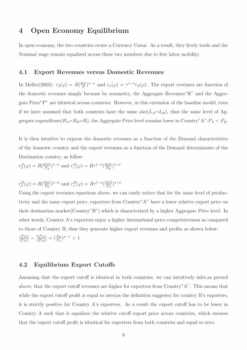
4 Open Economy Equilibrium

In open economy, the two countries create a Currency Union. As a result, they freely trade and the

Nominal wage remain equalized across these two members due to free labor mobility.

4.1 Export Revenues versus Domestic Revenues

In Melitz(2003): rd(ϕ) = R(p(ϕP)1−σ and rx(ϕ) = τ 1−σrd(ϕ). The export revenues are function of

the domestic revenues simply because by symmetry, the Aggregate Revenues”R” and the Aggre-

gate Price”P” are identical across countries. However, in this extension of the baseline model, even

if we have assumed that both countries have the same size(LA=LB), thus the same level of Ag-

gregate expenditure(RA=RB=R), the Aggregate Price level remains lower in Country”A”:PA < PB.

It is then intuitive to express the domestic revenues as a function of the Demand characteristics

of the domestic country and the export revenues as a function of the Demand determinants of the

Destination country, as follow:

rAd (ϕ) = R(p(ϕ)PA

)1−σ and rAx (ϕ) = Rτ 1−σ(p(ϕ)PB

)1−σ

rBd (ϕ) = R(p(ϕ)PB

)1−σ and rBx (ϕ) = Rτ 1−σ(p(ϕ)PA

)1−σ

Using the export revenues equations above, we can easily notice that for the same level of produc-

tivity and the same export price, exporters from Country”A” have a lower relative export price on

their destination market(Country”B”) which is characterized by a higher Aggregate Price level. In

other words, Country A’s exporters enjoy a higher international price competitiveness as compared

to those of Country B, thus they generate higher export revenues and profits as shown below:

rAx (ϕ)rBx (ϕ)

= πAx (ϕ)

πBx (ϕ)

= (PB

PA)σ−1 > 1

4.2 Equilibrium Export Cutoffs

Assuming that the export cutoff is identical in both countries, we can intuitively infer,as proved

above, that the export cutoff revenues are higher for exporters from Country”A”. This means that

while the export cutoff profit is equal to zero(as the definition suggests) for country B’s exporters,

it is strictly positive for Country A’s exporters. As a result the export cutoff has to be lower in

Country A such that it equalizes the relative cutoff export price across countries, which ensures

that the export cutoff profit is identical for exporters from both countries and equal to zero:

9

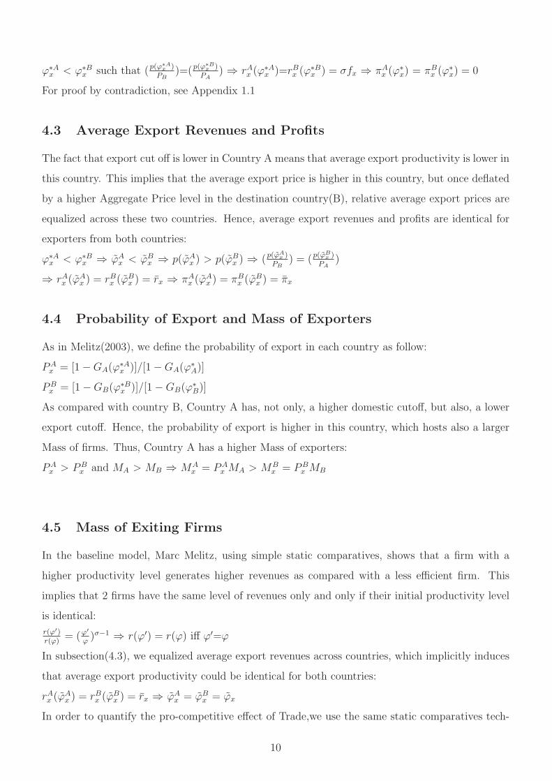
ϕ∗Ax < ϕ∗Bx such that (p(ϕ∗Ax )

PB)=(p(ϕ

∗Bx )

PA) ⇒ rAx (ϕ

∗Ax )=rBx (ϕ

∗Bx ) = σfx ⇒ πA

x (ϕ∗

x) = πBx (ϕ

∗

x) = 0

For proof by contradiction, see Appendix 1.1

4.3 Average Export Revenues and Profits

The fact that export cut off is lower in Country A means that average export productivity is lower in

this country. This implies that the average export price is higher in this country, but once deflated

by a higher Aggregate Price level in the destination country(B), relative average export prices are

equalized across these two countries. Hence, average export revenues and profits are identical for

exporters from both countries:

ϕ∗Ax < ϕ∗Bx ⇒ ϕAx < ϕB

x ⇒ p(ϕAx ) > p(ϕB

x ) ⇒ (p(ϕAx )

PB) = (p(ϕ

Bx )

PA)

⇒ rAx (ϕAx ) = rBx (ϕ

Bx ) = rx ⇒ πA

x (ϕAx ) = πB

x (ϕBx ) = πx

4.4 Probability of Export and Mass of Exporters

As in Melitz(2003), we define the probability of export in each country as follow:

PAx = [1−GA(ϕ

∗Ax )]/[1−GA(ϕ

∗

A)]

PBx = [1−GB(ϕ

∗Bx )]/[1−GB(ϕ

∗

B)]

As compared with country B, Country A has, not only, a higher domestic cutoff, but also, a lower

export cutoff. Hence, the probability of export is higher in this country, which hosts also a larger

Mass of firms. Thus, Country A has a higher Mass of exporters:

PAx > PB

x and MA > MB ⇒ MAx = PA

x MA > MBx = PB

x MB

4.5 Mass of Exiting Firms

In the baseline model, Marc Melitz, using simple static comparatives, shows that a firm with a

higher productivity level generates higher revenues as compared with a less efficient firm. This

implies that 2 firms have the same level of revenues only and only if their initial productivity level

is identical:

r(ϕ′)r(ϕ)

= (ϕ′

ϕ)σ−1 ⇒ r(ϕ′) = r(ϕ) iff ϕ′=ϕ

In subsection(4.3), we equalized average export revenues across countries, which implicitly induces

that average export productivity could be identical for both countries:

rAx (ϕAx ) = rBx (ϕ

Bx ) = rx ⇒ ϕA

x = ϕBx = ϕx

In order to quantify the pro-competitive effect of Trade,we use the same static comparatives tech-

10

nique as in Melitz(2003). In fact, we compare the revenues of an average productivity exporter

to those of an average productivity domestic firm on the destination market. Hence, we easily

determine, for each country, the number of domestic plants that are forced to exit the market due

to the entry of 1 exporter as follow:

rAx (ϕAx )

rBd(ϕB)

= ( ϕx

τϕB)σ−1 = θA ; rBx (ϕB

x )

rAd(ϕA)

= ( ϕx

τϕA)σ−1 = θB

These static comparatives reveal that the pro-competitive effect of Trade is more magnified for

Country”B”. In fact, the number of exiting domestic firms per average exporter(θ) is higher in this

country: ϕB < ϕA ⇒ θA > θB. Multiplying this number by the Mass of exporters, we get the Mass

of Exiting firms in each country: MBEX = θAM

Ax > MA

EX = θBMBx .

4.6 Equilibrium Mass of Firms and Average Profit in Open Economy

In each country, the Mass of firms in open economy is actually the Mass of firms that survive after

full liberalization of Trade. In other words,it is equal to the equilibrium Mass of firms in closed

economy net of the Mass of exiting firms.

In open economy,the Mass of firms remains larger in Country”A”, not only, because it was already

larger in closed economy,but also,due to the fact that the pro-competitive of Trade is less magnified

for this country, implying a smaller Mass of exiting firms:

MOA = MA −MA

EX > MOB = MB −MB

EX since MA > MB and MAEX < MB

EX

Average Profit in open economy is computed as follow:

πOA= πA + PA

x πx - PBx πx = πA + πx (PA

x − PBx )

πOB= πB + PB

x πx - PAx πx = πB + πx (PB

x − PAx )

Given that the probability of export is higher in Country”A” and average export profit is equalized

across countries, these 2 equations above show that while Free Trade increases average profitabil-

ity in the more efficient country(A),it makes firms in the other country(B),on average,less profitable.

4.7 GDP and Aggregate Profits in Open Economy

To assess the impact of Trade on the Output and the Aggregate Profit in each trading country, we

simply compare the value of these variables in Open economy to those obtained in Closed economy.

The equations below confirm that Free Trade makes the more efficient country(A) produce more

and enjoy higher Aggregate Profits and that these effects are completely opposite for the other

Country(B):

11

*GDPOA=GDPA + MA

x qAx - MAEX qA

=GDPA + PAX MA [RB(

p(ϕAx )

PB)−σ] - PB

x MB θB [RA(p(ϕA)PA

)−σ]

⇒ ∆ GDPA > 0

Under the following ”Stability Condition”: dqAdLA

= 0

(See Appendix for more details), we can write that:∆GDPA= f+(MA)

*GDPOB= GDPB + MB

X qBx - MBEX qB

=GDPB +PBX MB [RA(

p(ϕBx )

PA)−σ] - PA

x MA θA [RB(p(ϕB)PB

)−σ]

⇒ ∆ GDPB < 0

Note that ∆ GDPB =f−(MA) if this ”Stability Condition” is verified: dqBx

dLA= 0

*ΠOA= MO

A πOA = (MA −MA

EX) [πA + πx(PAx − PB

x )]

=(MAπA) + MAπx(PAx − PB

x ) - MAEX πA - MA

EX πx(PAx − PB

x )

⇒ ∆ΠA = (MA −MAEX) πx(P

Ax − PB

x ) - MAEX πA

=MOA πx(P

Ax − PB

x ) - MAEX πA > 0

∆ΠA = f+(MA) under the following ”Stability Condition”: drBxdLA

= 0

*ΠOB= MO

B πOB= (MB −MB

EX)[πB + πx(PBx − PA

x )]

=(MBπB) + MBπx(PBx − PA

x )- MBEX π

OB

⇒ ∆ΠB = −MBπx(PAx − PB

x ) - MBEX πO

B < 0

Note that ∆ΠB= f−(MA) since ∆ΠB = f−(MBEX) and MB

EX=θAPAx MA

These equations reveal that the variations of the Output and Aggregate Profits in Country”A” are

an increasing function of its size(LA). However, Country B’s Output and Aggregate profits would

react more negatively to full liberalization of Trade if the size of their trading partner (LA) was

larger. For more details, see Appendix 1.2

4.8 Tax rate Adjustment

Given that Public Expenditures are identical across countries and equal to 1 and that each Govern-

ment has to balance its budget, an increase/decrease in Aggregate Profits leads to a decrease/increase,

with the same magnitude, of the tax rate.

As a result, while Country A, which enjoys higher Aggregate Profits in Open economy, alleviates

the fiscal burden on its firms, Country B taxes more its economy after full openness to Trade to

12

compensate the decline in Aggregate Profits, as shown below:

Recall that the Gov’s budget constraint in each country is written:

Country”A”: tAΠA= 1 and Country”B”: tBΠB= 1

Taking Logs: Ln(tA)= - ln(ΠA) < 0 and Ln(tB)= - ln(ΠB) > 0

Hence, the equilibrium Tax rates in Open Economy are given by:

t∗′

A= t∗A + Ln(tA) ⇒ t∗′

A < t∗A

t∗′

B= t∗B + Ln(tB) ⇒ t∗′

B > t∗B

4.9 Analysis of the impact of Free Trade

Starting from a ”Closed Economy Equilibrium” where both countries have the same size(λ=LA

LB=1

and GDPA = GDPB), the same level of Aggregate Profits(ΠA

ΠB= 1) and the same tax rate(

t∗A

t∗B

= 1),

we have shown that Free Trade makes the more efficient country(A) produce more(GDPOA > GDPO

B )

and enjoy a relatively higher Aggregate Profit(ΠO

A

ΠO

B

> 1) and a relatively lower Tax rate(t∗′

A

t∗′

B

< 1).

Nevertheless, the variety gain is higher for Country B. In fact, its consumers enjoy a larger Mass of

additional varieties coming from Country A since this country has a higher Mass of exporters.

4.10 The Home Market effect still matters!

We have already proved that when both countries have the same size(λ=1), only Country A gains

from Trade in terms of production, Profitability and lower taxation. We have also shed light on

the fact that its gains,which are synonym of Losses for its trading partner(Country B), are an in-

creasing function of its size(LA).This implies that the variations of the relative GDP of Country

A, the relative Aggregate Profits of this country and the relative tax rate of Country B are all an

increasing function of the relative size of country A(λ). In other words, the larger the relative size

of Country A, the higher its gains and the bigger the losses for country B.

Hence, the Market size amplifies the initial impact of Trade on both countries!

13

5 FDI

5.1 FDI,the Trade-off

We have previously shown that the higher the relative Market size of Country”A”(λ), the higher

the relative fiscal pressure in Country”B”( tBtA).

Firms located in the less efficient Country(B) are facing the following Trade-off:

-Either continue to produce locally,thus avoid paying the fixed FDI cost (Fi) but accept to be

relatively more taxed on their profits.

-Or pay (Fi), relocate their production to Country A and enjoy lower fiscal pressure.

5.2 FDI function

FDIAB= ln( tBtA) - Fi

FDI from Country B to Country A is an increasing function of the relative size of this latter(λ). In

fact, the higher λ,the higher the relative Aggregate Profit in Country A and the higher the relative

tax rate in Country B. Thus, the stronger is the incentive for firms located in Country B to relocate

their production to the other Country to benefit from a more favorable tax regime.

FDIAB= ln( tBtA) - Fi >0 ∀ λ > λ∗

λ∗ represents the relative Market size cutoff beyond which the gain from lower taxation in Country

A exceeds the fixed FDI cost Fi. Therefore, when λ is high enough (λ > λ∗), the fiscal burden

becomes so heavy in Country B that all the firms escape it through relocating their entire production

to Country A where the huge gains from Tax alleviation exceed by far the fixed FDI cost. This is

clearly illustrated in the figure below:

14

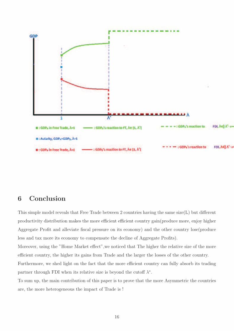
5.3 GDP reaction to Relative Market Size

When the relative market size of Country A is not too high (λ < λ∗), the tax rate is relatively lower

in Country A but the gain from fiscal alleviation is not that large to compensate the fixed FDI cost.

Hence, there is no FDI and countries freely trade only. Their respective Outputs in Open economy

can be written as follow:

∀λ ∈ [1, λ∗[, we have:∀λ ∈ [1, λ∗[, we have:

GDPOA= GDPA + ∆GDPA(

+λ)

GDPOB= GDPB + ∆GDPB(

−λ)

However,when λ is high enough (λ > λ∗), taxation becomes so favorable in Country A that all the

firms of Country B decide to relocate their production to Country A. In other words, the more

efficient Country(A) fully absorbs its trading partner through FDI as shown below:

∀λ ∈ [λ∗,+∞[, and since FDIAB=GDPB we get :

*GDPOA= GDPA + FDIAB =GDPA + GDPB

*GDPOB= GDPB - FDIAB = 0

15

6 Conclusion

This simple model reveals that Free Trade between 2 countries having the same size(L) but different

productivity distribution makes the more efficient efficient country gain(produce more, enjoy higher

Aggregate Profit and alleviate fiscal pressure on its economy) and the other country lose(produce

less and tax more its economy to compensate the decline of Aggregate Profits).

Moreover, using the ”Home Market effect”,we noticed that The higher the relative size of the more

efficient country, the higher its gains from Trade and the larger the losses of the other country.

Furthermore, we shed light on the fact that the more efficient country can fully absorb its trading

partner through FDI when its relative size is beyond the cutoff λ∗.

To sum up, the main contribution of this paper is to prove that the more Asymmetric the countries

are, the more heterogeneous the impact of Trade is !

16

7 Appendix

7.1 Appendix 1.1: Proof by Contradiction:

Let’s assume that ϕ∗Ax =ϕ∗Bx =ϕ∗x and compare rAx (ϕ∗

x) to rBx (ϕ∗

x):

rAx (ϕ∗x)rBx (ϕ∗x)

= (PB

PA)σ−1 > 1 ⇒ rAx (ϕ

∗

x) > rBx (ϕ∗

x)=σfx

⇒ πAx (ϕ

∗

x) > πBx (ϕ

∗

x) = 0

Hence, ϕ∗Ax has to be < ϕ∗Bx such that (p(ϕ∗Ax )

PB)=(p(ϕ

∗Bx )

PA)

This ensures that rAx (ϕ∗Ax )=rBx (ϕ

∗Bx ) = σfx. Thus, π

Ax (ϕ

∗

x) = πBx (ϕ

∗

x) = 0

7.2 Appendix 1.2: Stability Conditions

qA , qBx and rBx are increasing functions of the Aggregate Revenues (RA) and the Aggregate Price

level (PA) in country”A”.

An increase in the Market size of Country”A” (LA) has 2 opposite effects on these 2 determinants:

-it increases the Aggregate Revenues (RA), which shifts upward qA , qBx and rBx

-it decreases the Aggregate Price level (PA) because it implies a larger Mass of firms [M = f+(L)

and P = f−(M)].

Hence, the relative price (p(ϕ)PA

)−σ increases,which weakens the price-competitiveness and shifts down-

ward qA , qBx and rBx

We assume for simplicity that these 2 effects cancel out by writing : dqAdLA

= dqBxdLA

= drBxdLA

= 0

This assumption allows us to isolate the effect of relative market size variation on the magnitudes

of gains/losses in Country A/Country B.

17

8 References

Bernard AB, Jensen JB. 1995. Exporters, Jobs, and Wages in US Manufacturing: 1976-87. Brook-

ings Papers on Economic Activity: Microeconomics: 67-112.

Bernard AB, Jensen, JB. 1999. Exceptional Exporter Performance: Cause, Effect, or Both?

Journal of International Economics. 47(1): 1-25.

Demidova S. 2008. Productivity Improvements and Falling Trade Costs: Boon or Bane? Inter-

national Economic Review. 49(4): 1437-62.

Falvey,R.,D.Greenaway,and Z.Yu, 2004. ”Intra-industry Trade Between Asymmetric Countries

with Heterogeneous Firms”, GEP Research paper 2004/05

Helpman E., Melitz M. and Yeaple, S., 2003, Export vs. FDI, NBER working paper 9439

Krugman PR. 1980. Scale Economies, Product Differentiation, and the Pattern of Trade. Amer-

ican Economic Review. 70: 950-59.

Melitz MJ. 2003. The Impact of Trade on Intra-Industry Reallocations and Aggregate Industry

Productivity. Econometrica. 71: 1695-725.

Melitz MJ, Ottaviano G. 2008. Market Size, Trade, and Productivity. Review of Economic

Studies. 75(1): 295-316.

Mayer T. , Melitz MJ. and Ottaviano G. 2014. Market Size, Competition, and the Product Mix

of Exporters. American Economic Review. 104(2):495-536

Pavcnik N., 2002, Trade liberalization, Exit and Productivity Improvements: Evidence from

Chilean Plants, Review of Economic Studies 69, 245-276

Tybout, J., 2003, Plant and Firm-level Evidence on ”New” Trade Theories, in E. K. Choi and

J. Harrigan (eds) Handbook of International Trade Blackwell, Oxford.

18