The Heavy Costs of High Bail: Evidence from Judge

Randomization

Arpit Gupta∗

Christopher Hansman†

Ethan Frenchman‡§

August 18, 2016

Abstract

In the United States, roughly 450,000 people are detained awaiting trial on any given day,

typically because they have not posted bail. Using a large sample of criminal cases in

Philadelphia and Pittsburgh, we analyze the consequences of the money bail system by

exploiting the variation in bail-setting tendencies among randomly assigned bail judges.

Our estimates suggest that the assignment of money bail causes a 12% rise in the likeli-

hood of conviction, and a 6–9% rise in recidivism. Our results highlight the importance

of credit constraints in shaping defendant outcomes and point to important fairness con-

siderations in the institutional design of the American money bail system.

∗Email: ag2968@columbia.edu; Columbia GSB†Email: cjh2182@columbia.edu; Columbia University‡Maryland Office of the Public Defender§We thank Edward Morrison, Ilyana Kuziemko, Anne Milgram, and seminar participants at New York

University and Columbia Law School for helpful comments. We are grateful to Joel Mankoski and the Penn-sylvania Office of the Administrative Courts for data access, as well to the Center for Justice at ColumbiaUniversity for financial assistance.

1

1 INTRODUCTION

Roughly 450,000 people in the United States are held in jail awaiting trial on any given day.1

These individuals have not been convicted of a crime and are presumed to be innocent of the

charges for which they have been jailed. For the majority of defendants the barrier to release

is financial: they are unable or unwilling to post bail. Due to limited judicial resources,

defendants often remain incarcerated for months or years awaiting trial.2 Many defendants

who are detained on money bail before trial eventually choose to plead guilty in exchange for

release, rather than risking continued detention or an uncertain trial outcome.

There is significant evidence of a correlation between pretrial detention and both convic-

tion and recidivism, consistent with a direct impact of bail assessment on defendant outcomes

(for instance, Lowenkamp, VanNostrand and Holsinger (2013a), Lowenkamp, VanNostrand

and Holsinger (2013b), Phillips (2007), and Phillips (2008)). However, prior research has

struggled with causally estimating the impact of money bail due to the endogenous nature

of detention hearings.3 When judges determine whether to release an arrestee and the con-

ditions of such release, they consider, among other things, the facts of the case, the strength

of the evidence, and the arrestee’s criminal history, ties to the local community, and financial

resources. These factors may be related to factual guilt and render correlations between

money bail assessments and outcomes like convictions and recidivism difficult to interpret.

This paper investigates the causal impact of money bail on convictions and recidivism

using comprehensive court data from the two largest cities in Pennsylvania: Philadelphia and

Pittsburgh. By money bail, we refer to the requirement that criminal defendants post a cash

amount as bail in exchange for freedom before trial.4 In Philadelphia, defendants are assigned

bail at a centralized, 24-hour-a-day court presided over by arraignment court magistrates,

whom we refer to as judges for convenience. These judges differ in what we call severity, or

the propensity to assess bail. All else being equal, some judges assess money bail frequently,

while others do so sparingly. The Philadelphia system assigns defendants to bail judges in

1See http://www.bjs.gov/content/pub/pdf/jim14.pdf.2In our data, the median time between bail arraignment and trial is 200 days.3A notable exception is Abrams and Rohlfs (2011) who exploit an experiment in Philadelphia in the 1980s.4Other forms of bail may require non-monetary conditions, or only require the defendant to pay in the

event of a non-appearance.

2

an effectively random manner, creating a natural experiment that we exploit to determine

the role of money bail in determining defendant outcomes. We document that defendants’

assignment to more severe judges raises the probability of being assessed money bail for

reasons unrelated to other case factors, including defendant characteristics. This natural

experiment allows us to then study the implications of effectively exogenous impositions of

money bail on further defendant outcomes.

We find that the assessment of money bail is a significant, independent cause of convictions

and recidivism. In Philadelphia, criminal defendants who are assessed money bail are 12% (6

percentage points) more likely to be convicted. These effects appear to be driven by the subset

of cases where arrestees are detained due to their inability to post bail. We also investigate

money bail assessment and outcomes in Pittsburgh, where judicial assignment is based on

arrest location, and find similar results. We combine the Philadelphia and Pittsburgh samples

to gain statistical precision in examining the lasting negative effects of money bail after the

conclusion of the underlying criminal case. We document that the assessment of money bail

increases recidivism in our sample period by 6-9% yearly (0.7 percentage points).

Our results are primarily driven by whether money bail is required and not by the amount

of money bail. In other words, the assessment of money bail, rather than the bail size, appears

to cause convictions. A key implication of this finding is that simply lowering required bail

amounts will not ameliorate harms imposed by money bail. Our findings persist among a

number of subgroups—non-white defendants, those assigned a public defender, and male

defendants. We find estimates that are even larger among defendants charged with felonies,

though we do not reach statistical significance in that sample. This suggests that our effects

are not merely driven by convictions for petty crimes.

We do not attempt to isolate the exact channel by which money bail causes convictions

and recidivism. Money bail, as a source of pretrial detention, imposes significant costs on de-

fendants. As the Supreme Court wrote in Gerstein v. Pugh (420 U.S. 103, 114 [1975]) pretrial

detention “may imperil the suspect’s job, interrupt his source of income, . . . impair his family

relationships [and affect his] ability to assist in preparation of his defense.” Many defendants

who are detained on money bail before trial may consequently choose to plead guilty to avoid

3

or minimize further detention. Prosecutors commonly offer detained defendants a plea of

“time-served,” where defendants will receive credit for time already spent in detention and

will therefore be released immediately upon conviction. Other potential channels include the

difficulty detained defendants have communicating with their counsel and properly prepar-

ing a defense; changes in behavior among various institutional actors such as prosecutors,

defense attorneys, judges, and jurors toward defendants who are incarcerated pretrial; the

limited opportunity for detained arrestees to participate in diversionary programs and other

resolutions not resulting in convictions; and the financial strain of making bail.5 Money bail

may also directly influence recidivism through the harms of pretrial incarceration imposed

upon those those unable to make bail, post-trial incarceration following conviction, or the

stigma of conviction.6

Despite the multiplicity of possible channels, we emphasize that our results provide novel

evidence of a causal role of money bail and pretrial detention on defendant outcomes. The

relationship between money bail, conviction, and recidivism suggests a strong interaction

between poverty and the criminal justice system. A large literature has examined the credit

constraints facing American households that make even small money bail amounts difficult to

post (see Lusardi, Schneider and Tufano (2011)). While it is feasible that money bail could

impact convictions among those with sufficient liquid assets to post bail, it is more likely that

these effects come primarily from the credit-constrained. It is important to note that a large

majority of arrestees in our sample qualified for representation by the public defender, and

therefore are presumably indigent.

The interactions between money bail and subsequent defendant outcomes pose substan-

tive legal issues. From a liberty perspective, these relate to the incarceration of presumptively

innocent people and the basic assumption that convictions reflect only the merits of the un-

derlying case. Bail also raises equality issues related to the requirement of equal access to

justice and the prohibition against wealth discrimination. Racial is a further concern, and

we find evidence consistent with racial discrimination in bail setting: non-white defendants

5Though bail bondsmen can front bail amounts in exchange for a collateral value which is typically 10%,even these relatively smaller collateral values may be out of reach for criminal defendants facing liquidityconstraints. In Philadelphia, the court may accept 10% of the bail amount.

6See, e.g., Baylor (2015);Appleman (2012); Phillips (2008).

4

are more likely to be assessed money bail, yet less likely to be found guilty. However, this

correlation is suggestive, and may reflect unobserved factors that are correlated with race.

Our findings also raise institutional design questions regarding the American money bail

system as a whole. The money bail system in Philadelphia and Pittsburgh has a lot in

common with the money bail systems used in many cities around the country, such as New

York and Baltimore. Arrestees see a judicial officer who determines whether to release a

person pending trial or impose money bail. Those people who are unable to pay their bail

have the opportunity to plead guilty or remain in jail until trial. In systems to the one in

Philadelphia and Pittsburgh, our research suggests that money bail causes convictions and

recidivism.7

One suggested solution to the perceived inequities of pretrial detention is the adoption of

empirical pretrial risk assessments. Such tools, based on multivariate models built from large

sets of defendant data, create recommendations for release or conditions of release. Despite

the use of such assessment tools in Philadelphia and Pittsburgh in the time period covered

by our analysis, judges varied widely in assessing bail amounts for similar defendants, calling

into question the ability of such tools to rein in judicial discretion.

To contextualize our findings on guilt and recidivism, we examine whether the assessment

of money bail induces defendants to appear at trial, the stated purpose of the money bail

system. As we are unable to explicitly observe defendants failing to appear, we construct

two proxies based on the issuance of bench warrants. While these proxies are imperfect —

both likely understate the true number of failures to appear — we find no evidence that

money bail increases the probability of appearance. These results should be interpreted

as preliminary, and a more nuanced study of court appearances using more complete date

is necessary. Nevertheless it is notable that we are unable to find an obvious impact of

money bail. Pretrial detention is expensive. Philadelphia spent an estimated $290 million on

jailing in 2009, and 57% of the daily jailed population was detained awaiting trial (Eichel,

2010). Rationalizing the costs imposed by money bail (via detention costs, convictions and

7Of course, the impact may differ depending on the population. For instance, in certain places, defendantsmay be relatively well-off and have the general ability to pay money bail. In such a place, we would expectthat the causal impact of money bail would be lower than in Philadelphia, where many people are too poorto pay their bail.

5

recidivism) requires substantial compensating public benefits, and we find no evidence that

such benefits exist.

Our research has a close connection to the literature on pretrial justice.8 There is a large

body of evidence suggesting that pretrial custody status is associated with the ultimate out-

comes of criminal cases, with detained defendants consistently faring worse than defendants

at liberty (See ABA Standards for Criminal Justice: Pretrial Release 29 (3d. ed. 2007)). Past

work has uncovered the correlation between money bail, pretrial detention, and conviction

(e.g. Phillips (2007), Phillips (2008)), and examined other policy considerations regarding the

design of pretrial detention systems (See Lowenkamp, VanNostrand and Holsinger (2013a),

Lowenkamp, VanNostrand and Holsinger (2013b), Bechtel et al. (2012), and Phillips (2012)).

In the economics literature, beyond Abrams and Rohlfs (2011), our work is most closely

related to papers utilizing random assignment of judges within the criminal justice system

such as Kling (2006), Doyle Jr (2007), Doyle Jr (2008), Mueller-Smith (2016) and Aizer and

Doyle (2015), as well as in other contexts, such as Chang and Schoar (2007), and Dobbie and

Song (2015). Especially relevant is concurrent and complementary work by Stevenson (2016),

which uses a similar approach in Pennsylvania to examine the impacts of pretrial detention

on case outcomes. Our work differs in that we also examine recidivism and establish a long-

term negative outcome of incarcerations spells. We also differ in that our approach focuses

on the decision of judges to set money bail, rather than the detention status of defendants.9

Our paper is structured as follows: Section 2 presents legal background on the money bail

system in Philadelphia and Pittsburgh, Section 3 explains our data and empirical strategy,

Section 4 contains estimation results, and Section 5 concludes.

2 LEGAL BACKGROUND AND BAIL HEARINGS

2.1 Legal Background

Any person who is arrested without a warrant is entitled to a hearing within 48 hours of

arrest, see Cnty. of Riverside v. McLaughlin (500 U.S. 44, 56 [1991]) and (Gerstein, 420 U.S.

8The Pretrial Justice Institute has created an exceptionally detailed bibliography, available at:http://www.pretrial.org/wpfb-file/pji-pretrial-bibliography-pdf/.

9In principle, guilty pleas may be affected by bail setting even when bail is posted due to the financial costof making bail. Our Table 5 examines the consequence of bail setting on the full interaction of outcomes ofpre-trial detention and case guilty.

6

at 114). At this hearing, a judicial officer must determine whether there is probable cause for

the arrest prior to the imposition of “any significant pretrial restraint of liberty.” (Gerstein,

420 U.S. at 125). Across the country, this initial appearance has evolved into a “hearing at

which the magistrate informs the defendant of the charge in the complaint, and of various

rights in further proceedings, and determines the conditions for pretrial release.” Rothgery

v. Gillespie Cnty, Tex (554 U.S. 191, 199 [2008]).

At a bail hearing, judges have a number of options available to them:

1. Release on Recognizance (ROR) — Requires the defendant only to agree to appear at

a later date

2. Non-Monetary Conditions — Allows some non-monetary restriction to be placed on

the defendant, such as pretrial supervision or a curfew

3. Unsecured Monetary Condition — Written agreement to be liable for a fixed financial

payment, akin to a promissory note.

4. Secured Monetary Condition — Defendant must satisfy a financial condition paid to the

court either directly, through a bail bondsman, or other collateral such as real property,

in order to secure release

5. No Bail — Defendant is to be held pending trial

A variety of constitutional and legal protections constrain the discretion of judicial officers

in determining whether to detain or release a defendant and what conditions to place on

such release. First, pretrial liberty is a fundamental right independently guaranteed by the

Constitution. See Foucha v. Louisiana (504 U.S. 71, 80 [1992]); U.S. v. Salerno (481 U.S.

739, 750 [1987]). “In our society liberty is the norm, and detention prior to trial or without

trial is the carefully limited exception.” (Salerno, 481 U.S. at 755). Therefore pretrial

detention must be “narrowly focus[ed]” to the government’s “compelling” interests in public

safety and return to court. (See Salerno, 481 U.S. at 750-51) and Stack v. Boyle (342 U.S.

1, 4 [1951]); ABA Standards for Criminal Justice: Pretrial Release 37 (3d. ed. 2007). In

determining whether to release a defendant, and what conditions to place on such release,

7

the judicial officer must make an individualized assessment of the case and defendant. (See

Stack, 342 U.S. at 5).

Bail also raises issues covered under the Equal Protection Clause of the Fourteenth

Amendment to the Constitution, which has been interpreted to prohibit “punishing a person

for his poverty.” Bearden v. Georgia (461 U.S. 660, 671 (1983)). Persons may not be incar-

cerated solely due to their inability to make a payment. (See Bearden, 461 U.S. at 671) and

Tate v. Short (401 U.S. 395 [1971]); Williams v. Illinois (399 U.S. 235 [1970]); and Smith v.

Bennett, (365 U.S. 708, 709 [1961]). For this reason such payments must take into account a

person’s financial resources.

These guarantees find a statutory parallel in the Pennsylvania Rule of Criminal Proce-

dure 523, which explicitly requires magistrates to consider arrestees’ financial resources when

setting money bail.

2.2 Bail Hearings

In Pennsylvania, a magistrate presides over the initial appearance of an arrestee. In Philadel-

phia particularly, a centralized bail court operates 24 hours a day. Defendants from across the

city appear before one of a team of appointed magistrates who conduct the initial detention

hearing. Magistrates generally preside via CCTV over satellite locations in the city where

arrestees are held. The centralized location, high case load, constant process, and rotating

magistrate calendar result in the effectively random assignment of defendants to magistrates

(an assumption we test). Importantly for our purposes, magistrates in Philadelphia only

preside over the initial appearance; they do not preside over subsequent hearings or trials.

As a result, magistrates only impact the case at the bail assessment, and not at later stages.

In Pittsburgh, magistrates are elected to a six-year term to serve in a district court, which

administers a particular geographic section of Allegheny county. A single magistrate handles

the majority of the arrests that occur within their jurisdiction, although many arrestees are

seen by other magistrates during weekends, nights, and other periods when the presiding

magistrate is not in service. As a result, defendants in Pittsburgh are assigned to judges in

part based on the location and time of their arrest.

8

At the pretrial detention hearing in both Pittsburgh and Philadelphia a magistrate hears

information from the defendant (or the defendant’s counsel) and the prosecutor relevant to

the defendant’s flight risk and public safety. This information includes the many factors set

forth in Pennsylvania Rule of Criminal Procedure 523, such as: the nature of the offense,

the strength of the evidence, the defendant’s financial resources, family and community ties,

criminal record, and prior failures to appear. These hearings typically last only a few minutes.

In Philadelphia and Pittsburgh, magistrates also employ a empirical risk assessment tool,

meant to standardize decisions regarding pretrial detention.10

Should money bail be set, detainees may only secure their release through the satisfaction

of its financial terms. In Philadelphia, detainees may post 10% of the money bail amount

directly to the court.

Detainees who cannot afford the financial condition of their release remain incarcerated

for months or even years awaiting trial. Detainees have the opportunity to move for a

reduction in their money bail after the initial hearing. We focus on the initial assessment

of money bail, as it is the product of a randomized judicial decision, and find this decision

is influential in determining the final amount the defendant is required to pay, regardless of

later modifications.

The timeline of defendant actions around the release determination varies from state to

state. In Pennsylvania, the detention hearing precedes the entry of the plea, ensuring that

the magistrate’s assessment of money bail is a factor in the defendant’s plea decision from

the beginning.

3 DATA AND EMPIRICAL STRATEGY

3.1 Data Summary

We obtained comprehensive criminal data from the Administrative Office of the Pennsylvania

Courts for 2010-2015. These include records from the local magistrate courts as well as

10Although we find that these tools do not eliminate the exercise of wide judicial discretion.

9

subsequent judicial and defendant decisions from the higher Court of Common Pleas. In

Philadelphia, a separate municipal court system typically handles initial arraignments.

Table 1 summarizes the data for our focal region of Philadelphia, where we are best able

to establish judicial randomization, as well as Pittsburgh—the second largest jurisdiction in

the state. Our data contain information about the entire history of detention determinations

and money bail assessments on criminal defendants (although we focus on the money bail

amount resulting from the initial hearing); disposition information on the list of charged

offenses; bench warrant information; and final sentencing outcomes for individual defendants.

Our first appendix table, Table A1, contains the top 10 most common offenses and basic

characteristics of the cases associated with those offenses.

3.2 Empirical Strategy

A simple approach to addressing the role of money bail would be to run the OLS regression:

Guiltit = α+ βBailit + εit

where Bailit is an indicator for whether or not individual i is assigned money bail in time

t. Table 2 illustrates this strategy. Column 1 suggests that being assessed money bail results

in a 1.4 percentage point increase in the probability of pleading guilty. As shown in column 3,

this goes up to 4.3 percentage points after adding a battery of additional controls, including

gender, race, age, and offense fixed effects. This relationship is confirmed in column 4, where

we focus on the log of the bail amount instead of the indicator for money bail assessment.

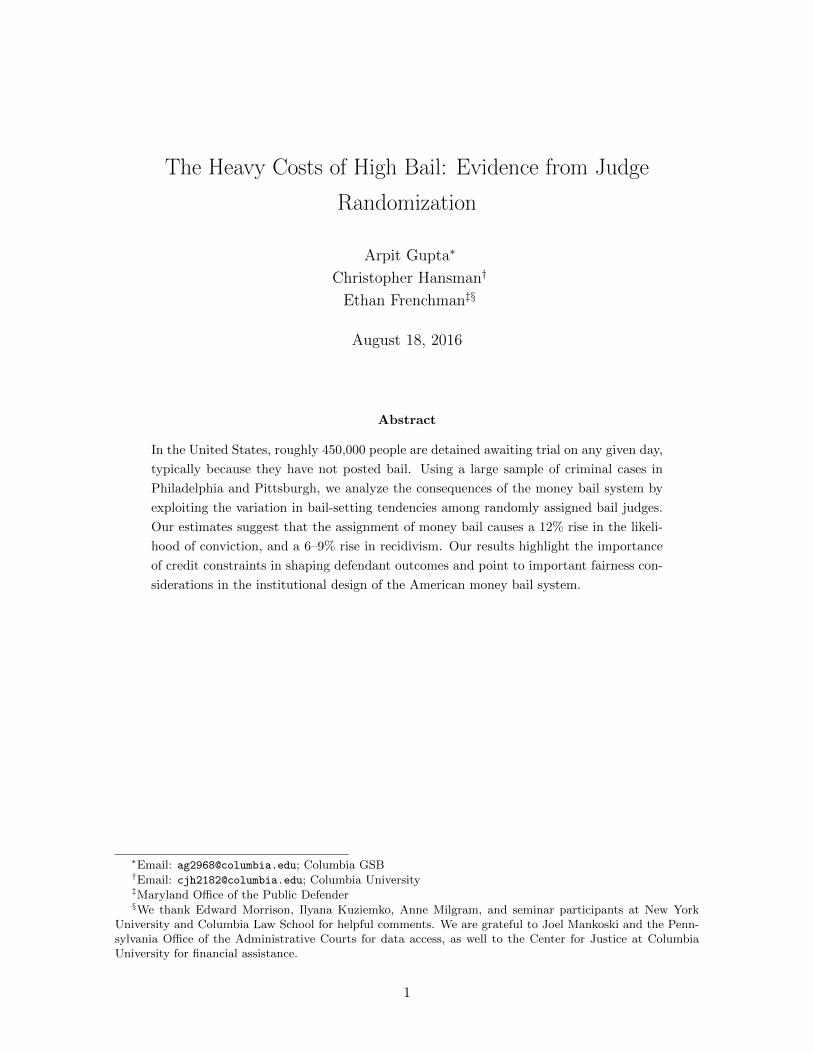
Figure 1 provides an illustration of this correlation for one offense: possession of marijuana.

Defendants charged with this offense are substantially more likely to be found guilty when

assessed money bail.

While these estimates are consistent with a causal interpretation that higher bail amounts

induce convictions, they are also consistent with a spurious correlation resulting from the

endogenous bail assessment. Recall that bail assessments are not made randomly, but are

intended to be calibrated against the nature of the offense, the flight risk of the individual,

10

and even the strength of the case. As these factors are also likely to be associated with the

underlying guilt of the defendant, the results from Table 1 may not reflect a causal role of

bail.

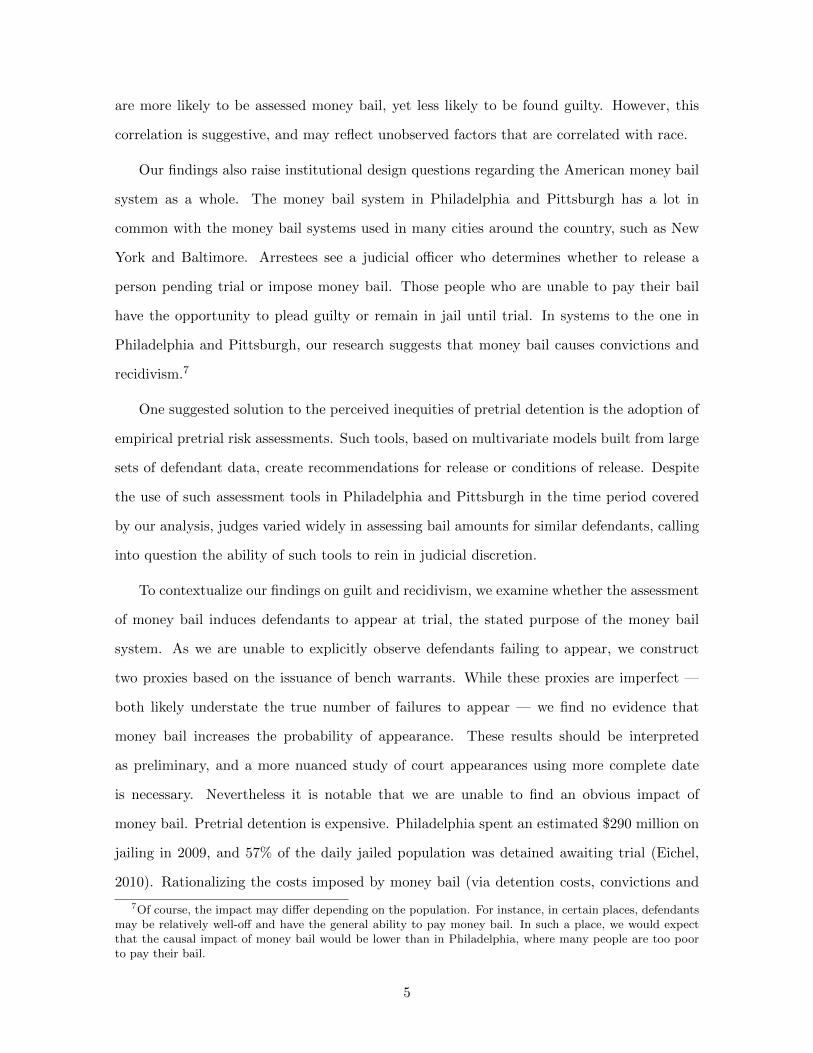
Concerns about the endogenous assignment of bail are heightened by the results shown

in Panel A of Figure 2, which displays the coefficients from a regression of money bail on

various covariates. While there is a raw univariate correlation with guilt, the assessment of

money bail is also associated with gender, race, and prior cases. The correlation of money

bail with these covariates is indicative of the endogenous initial assignment of money bail.

The goal of our empirical strategy is to address this endogeneity concern using the effec-

tively random assignment of defendants to judges. Bail judges differ widely in how they treat

similarly situated defendants. Some judges are far more likely to impose money bail, and

to impose money bail in greater amounts, than other judges. In other words, certain judges

over time tend to set bail when other judges would not, all else being equal. We refer to each

judge’s propensity to set money bail as the judge’s severity. Therefore, a defendant’s chances

of receiving money bail depend on the severity of the bail judge, not just the characteristics

of the case and the defendant. Because defendants are close to randomly assigned to bail

judges, the judicial assignment serves as the treatment in a natural experiment. We isolate

the effect of the severity of the bail judge in setting money bail to determine the role of money

bail on defendant outcomes.

The coefficients plotted in Panel B of Figure 2 reflect our attempt to isolate the impact

of random judicial assignment on guilt. This figure shows the relationship between a battery

of covariates and the component of money bail that is due only to judicial severity. They are

created by regressing several covariates on the linear prediction of money bail on a judicial

severity measure described below. None of the covariates appear to be related to the fraction

of variation in money bail that is driven by judicial variation, indicating random assignment.

By contrast, our outcome variable of guilt is associated with our instrument—showing how

the judicial assignment of bail can produce causal estimates of the impact of money bail.

Conceptually, our identification strategy is to isolate the impact of the judge on the

probability that an individual is assigned money bail. One approach would be to use judge-

specific fixed effects to instrument for whether a defendant is assigned bail. This would

11

involve estimating a first stage, for individual i in court c with judge j, of:

Bailicjt = α+ γc + δj + vit

and estimating the effect of Bailicjt on guilt in a second stage, where δj are judge fixed

effects. However, the assumptions required for IV estimation via two-stage least squares

may be violated in finite samples because of a mechanical correlation in the first stage. The

estimated judge fixed effects are essentially an average across defendants, and with a small

number of cases each defendant contributes significantly to the average. As discussed above,

a defendant’s own bail assessment is likely to be correlated with unobserved factors that are

associated with guilt. If this is true, then averaging that bail assessment with a finite number

of other defendants’ assessments will not in general eliminate the correlation.

A solution to this problem in the literature (e.g., Dobbie and Song (2015)) involves

estimating a leave-out mean for each defendant:

Zicjt =1

ncjt − 1

(ncjt∑k=1

(Bailk)−Baili

)− 1

nct − 1

(nct∑k=1

(Bailk)−Baili

)

which we refer to as judicial severity. The first term of Zicjt is simply the average of Bailkcjt

for all individuals faced by judge j except for i (all k 6= i). The second term subtracts out

the average of Bailkcjt at the court c, once again omitting individual i. Intuitively, Zicjt

is simply judge j’s average relative to the court’s average, computed using everyone but i.

Because Zicjt is computed without using individual i, there is no mechanical correlation. This

leave-out mean is then used as an instrument in place of judge fixed effects.

While the exposition above demonstrates a judge-level leave-out mean, our preferred

instrument is slightly more granular. To account for possible non-random assignment by

offense we compute a leave-out mean at the offense-judge level. That is, the average for

a judge for a given offense type, relative to the court average for that offense. For this

instrument, we need only assume that individuals of the same offense category are randomly

assigned to judges. Our primary specifications depend on a version of the instrument in

12

which Bailit is defined as the binary decision of whether to assign bail or not. However, we

also examine alternative continuous measures, including log(1+ bail amount).

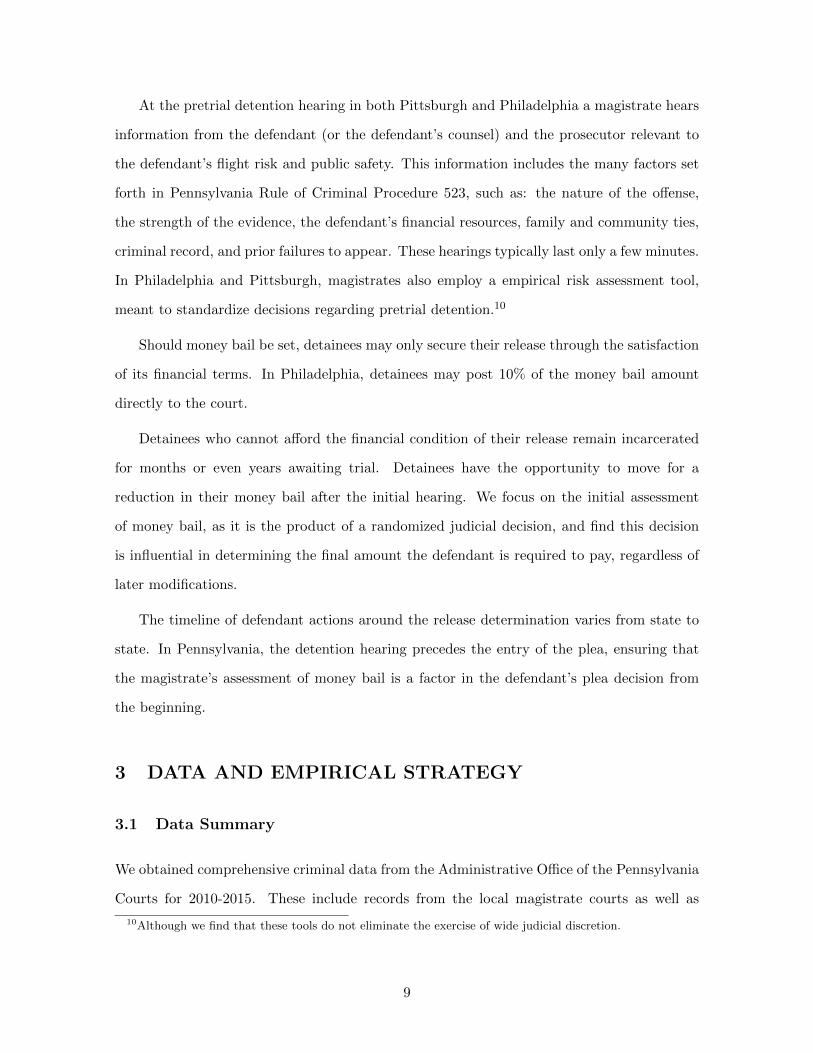
Panel A of Figure 3 illustrates our estimate of judicial severity against the log bail amount,

showing that judge severity is highly predictive of bail amounts faced by criminal defen-

dants11. Panel B shows that our judge severity measure is consistent over time, suggesting

that judge severity is driven by idiosyncratic personal factors rather than temporary shocks

or case characteristics (judge severity is even consistent across different offices when judges

move to serve in other jurisdictions).

In our main specifications, we instrument for Bailicto with Zictjo, our measure of judge

severity taken from a within offense measure:

Guilticto = α+ βBailicto +X ′ictoδ + ηcto + εictjo

Bailicto = α+ γZictjo +X ′ictoζ + ρcto + victjo

with errors clustered at the jurisdiction-judge-year level. Our identifying assumption,

taken from judge randomization, is that:

corr(Zictjo, εictjo) = 0.

In the next section, we provide supporting evidence for this assumption.

It is important to note that these results are created using an instrumental variable

approach that focuses on criminal defendants induced to pay money bail as a result of judicial

severity. In other words, we estimate a local average treatment effect (LATE) identified on the

basis of individuals for whom changes in bail assessment resulting from variation in judicial

severity impact guilty pleas. These defendants are more likely to represent criminal cases

for which there is more scope for judicial variation in bail setting. Nevertheless, we do find

11 We measure judicial severity using a leave-out-mean of the log[1 + Money Bail Amount] at the judge-yearlevel, relative to the leave-out-mean average at the court in the same year. These computed judicial measuresare then regressed against individual measures of log bail with fixed effects for the month of arraignment.The resulting residuals are averaged at the judge-year level and the average log bail amount is added to eachresiduals. Panel A contrasts the averaged measure of judicial severity against average log bail amounts at thejudge-year level. Panel B compares the averaged measure of judicial severity in one year against the samejudge’s measure the previous year.

13

that our results persist in a number of important subcategories (including defendants facing

felonies), and our results are quite comparable in both Philadelphia and Pittsburgh. These

checks suggest that our results have external validity outside of the precise jurisdictions we

examine.

3.3 Randomization Check

Though our analysis of the judicial assignment process in Philadelphia leads us to expect

close-to-random assignment of cases across judges, we check this assumption by examining

the association between our leave-out-mean estimator and a series of defendant covariates in

Table 3. Column 1 illustrates the means of the covariates we analyze. Column 2 regresses

our instrument against each covariate in isolation with no additional controls and reports

the coefficient. Column 3 regresses our instrument against all covariates and includes fixed

effects for the most severe offense among the defendant’s charges. Column 4 adds additional

month-of-arraignment fixed effects.

Across all specifications, we find strong evidence for random assignment. F-statistics of

the joint significance of covariates we test against our instrument are 0.54 with only month

fixed effects and 0.34 when including both month fixed effects and offense controls.

4 RESULTS

4.1 IV Results

Table 4 presents our main results from Philadelphia. The first column shows the first stage—

a regression of our instrument of judicial severity against a binary indicator of whether the

defendant was assessed money bail. While defendants are on average likely to receive money

bail (62%), we find that judicial factors also play a large role. Our first stage suggests strong

instrumental validity: being assigned to a more severe judge results in defendants facing a

higher likelihood of being assessed money bail. Given the close-to-random assignment to

judges and the lack of correlation between our instrument and observable defendant charac-

teristics, we interpret this first stage as indicating that judicial severity provides effectively

exogenous variation in money bail.

14

Column 2 presents the reduced form—a direct regression of our instrument of judge

severity against the outcome of guilt. Although this relationship will be attenuated—because

not all people who receive a severe judge are impacted by way of higher bail amounts—the

strong and significant relationship in the reduced form indicates a causal relationship between

judge severity and conviction.

The third column scales the reduced form by the first stage to produce our instrumental

variables estimate of the relationship between money bail and conviction. Our estimate

suggests that defendants who are required to pay money bail as a result of being assigned to

a severe judge are 6 percentage points more likely be convicted. Given a baseline guilt level

of 50% in our sample, our estimate suggests that the presence of money bail increases the

likelihood that a defendant is found guilty by about 12%.

This estimate is large, tightly identified through our measure of judicial severity, and

suggests a powerful role for money bail in inducing convictions. Our data do not permit

complete analysis of whether convictions result from plea bargains or trials. However, we

have strong results when focusing on cases in which we can explicitly observe plea behavior,

and cases proceeding to trial appear in our sample only rarely. We believe our estimates are

primarily driven by defendant plea behavior.

Table 4 also provides suggestive estimates regarding the role of race in case outcomes.

Column 1 shows that non-white defendants are 1.4 percentage points more likely to be as-

sessed money bail. However, columns 2 and 3 show that non-whites are less likely to be

found guilty of crimes. While these results should not be interpreted causally, as they do

not exploit judicial randomization and may reflect non-racial factors associated with race,

they are consistent with racial bias in the criminal justice system. They are also consistent

with other mechanisms of the legal process. For instance, prosecutors or judges may correct

for an initial bias in arrest by dismissing or differentially pursuing cases involving non-white

defendants. While our data do not permit a complete analysis of racial bias in bail setting,

this remains an interesting avenue for future research.

We next detail the relationship between money bail, pretrial detention, and convictions.

There are a number of paths a defendant may take following the initial bail assessment. We

15

consider a categorization of four possible paths in a criminal case: defendants may be detained

and found guilty, detained and found not guilty, released and found guilty, or released and

found not guilty. Table 5 attempts to analyze the impact of money bail on the flow of

defendants between these four categories. Each of the four columns presents an IV regression

(as in column 3 of Table 2) with one of those categories as the dependent variable. As the

dependent variables across the four columns are mutually exclusive and exhaustive, one of the

columns is redundant, in the sense that the coefficients in any row must sum to 0. However,

examining all four columns provides a useful picture of the impact of money bail on the path

defendants take from bail assessment to their ultimate case outcome.

Since defendants not receiving money bail are presumptively released, we can assume that

the imposition of money bail is unlikely to increase the number who are released. Fort this

reason, we observe that the judicial assignment of money bail reduces the outcome of release

both in column 2 (release and guilty) and column 4 (release and not guilty). Although we are

not able to precisely estimate the effects in either column, Table 5 suggests that money bail

decreases the probability that a defendant is released and ultimately found guilty by nearly

10 percentage points and decreases the probability that a defendant is released and found

not guilty by nearly 8 percentage points.

The reduction in the released population must be matched by an increase in the detained

population. Nearly the entire increase falls into the first column: we see a 16 percentage

point increase in the outcome of detention and guilt. In other words, money bail increases the

probability of detention for those who would be counterfactually released, and the majority

of the population that is detained as a result of money bail is ultimately convicted.

4.2 Robustness

For robustness, we provide a number of additional checks. Table 6 explores our main IV

specification as illustrated in column 3 of Table 4 for different subsamples—being charged

with a felony, having a public defender, being male, and being non-white. While none of

these estimates are statistically different from our main estimates, it is noteworthy given

our findings on race discussed above that our IV point estimate for non-whites is higher,

16

at 8.3 percentage points. Our finding on felonies, an 8.1 percentage point increase, is not

precisely estimated but is high in magnitude and suggestive that instances of guilt induced

by higher bail are not for low-level crimes exclusively. Being convicted of a felony typically

results in severe long-term impacts on defendant outcomes, including opportunities for future

employment and voting status.12

Tables 7 and 8 explore alternate specifications of our judge severity measure. Table 7 uses

the log of 1 plus the bail amount, effectively using both the intensive and extensive margins.

Table 8 uses the log of the bail amount, conditional on being assigned money bail—that is,

only the intensive margin. In Philadelphia, we find no evidence that the intensive margin

matters, only the extensive margin of being assessed money bail.

Next, we turn to Pittsburgh. As discussed in section 2, the nature of judicial assignment

in Pittsburgh and the rest of the state is not as clean and does not permit a straightforward

causal estimate. Rather than a central courtroom that handles all cases, individual magistrate

judges are elected to districts in the city and are principally responsible for cases within that

jurisdiction. Our judge measure therefore captures the variation arising from the difference

between the principal judge and other judges, which account for 20–30% of cases in districts,

typically due to the principal judge being absent on a weekend, night, vacation, or for some

other reason. Our identifying assumption is that case loads, conditional on observables, do

not differ between the principal judge and other judges in a given district.

A randomization check in Appendix Table A2 suggests that there is non-random judicial

assignment in Pittsburgh, with an F-statistic of 4.74 for various defendant characteristics

regressed against a measure of judicial severity within Allegheny County. Nonetheless, to

establish robustness of our primary finding outside of the city of Philadelphia, we attempt

a version of our main specification in Pittsburgh in Table 9. Remarkably, given the extent

of non-random assignment, we find estimates that are virtually identical in Pittsburgh—in

column 3, we see a 6.4 percentage point increase in guilt as a result of money bail assessment.

Due to the comparability of the Pittsburgh and Philadelphia samples, in subsequent analysis

on recidivism we combine the two samples in order to maximize statistical power.

12Though convicted felons can vote in Pennsylvania.

17

Appendix Table A3 examines how our results vary across the distribution of bail amounts.

To avoid an endogenous assignment of bail amounts, we first categorize offense categories

according to the average bail amount into quartiles. Next, we estimate our main IV analysis

within each quartile of bail assessment. Interestingly, we find that our results appear to be

largest in the first quartile, where bail amounts are lowest. This suggests that the imposition

of money bail, even when bail amounts are low, is sufficient to cause convictions.

Appendix Tables A4 and A5 focus on the top five most common offenses within felonies

and misdemeanors. Table A4 highlights the extensive margin and shows coefficients from our

main IV specification run on individual offenses (without offense fixed effects). Interestingly,

our results appear among various categories of theft—retail theft, receiving stolen property,

and retail theft (misdemeanor). Our results are somewhat lower and do not reach signifi-

cance for drug offenses, DUIs, and gun possession charges. These results are comparable to

Stevenson (2016), who also finds substantial results among those categories and lower effects

on drug and other charges.

Table A5 examines the intensive margin—whether changes in the intensity of bail matter

given that bail was set. Interestingly, we only find effects here among gun possession misde-

meanors. It is possible that the effect could be driven by the relatively high average bail in

this category (around $11,000). Though other offense categories also carry high bail amounts

(such as aggravated assault), they typically also carry greater consequences which may deter

defendants from pleading guilty. Future work will attempt to analyze why responses to bail

setting appear to be particularly high in some offenses more than others, which may assist

in adjusting pretrial detention standards.

4.3 Other Outcomes

4.3.1 Recidivism

We next look at recidivism, which we explore in Table 10. Existing literature has documented

the role of incarceration on future criminal activity.13 There are a variety of mechanisms

which appear to drive this relationship, including the negative impact of incarceration on

13See for instance Mueller-Smith (2016) and Aizer and Doyle (2015).

18

labor market outcomes (encouraging illegal income seeking), family disruption, loss of human

capital, and peer effects resulting from associations with other detainees.

We extend this literature by examining the role of money bail on future criminal activity.

There are a number of channels through which money bail in particular might cause recidi-

vism. As our results from section 4.1 show, money bail causes convictions, which in turn may

entail incarceration and subsequent effects. Even without additional convictions, money bail

may impact future criminal activity via job loss during pretrial detention, financial hardship

caused by raising funds to make bail, or other factors. Our data do not permit, and we do not

attempt, a complete separation of the various mechanisms linking bail assessment to future

criminal activity.

We follow some of the prior literature in this area by restructuring our data into a yearly

panel format. Our main specification follows the first criminal offense committed by defen-

dants in our data and estimates:

Recidivismi,t+y = α+Xi,t + µy + µt + βBaili,t + εi,t+y

Where Recidivismi,t+y is a binary indicator equal to one if the defendant is charged with

a crime in the yth calendar year after his or her initial charge (where the initial charge year is

denoted by t). Xi,t is the full list of defendant controls previously included (these include the

age, race, and gender of the defendant; along with controls for the criminal charge) which are

taken in the calendar year of criminal charge. µy is a calendar year fixed effect; µt controls

for the month of arraignment. Baili,t is an indicator for whether the defendant was required

to post money bail, and is instrumented for using our judicial severity measure. β remains

the key causal variable of interest, capturing the role of exogenous bail assessments on future

recidivism. Our yearly defendant panel begins in the calendar year in which defendants enter

our data as a result of initial charge, and ends in 2015 (the last year for which we have

criminal charge data). Standard errors are clustered at the defendant level.

The base rate of yearly recidivism in our sample (around 12% in Philadelphia) along with

the standard errors of our IV estimates result in some statistical imprecision in our estimate

in Philadelphia. In column 1 of Table 10, we examine the role of money bail assessment

19

on the yearly probability of future criminal behavior. Though the estimate of 0.007 is quite

large economically (corresponding to a 0.7 percentage point yearly increase in the probability

of committing future crime, or a 6% increase), we are unable to statistically distinguish this

result from zero. In order to gain statistical precision, in column two we expand our sample to

a “Combined Sample” which includes data from both Pittsburgh and Philadelphia. Though

the judicial assignment process is not as random in Pittsburgh as in Philadelphia, we find

quite comparable results in both localities in most of our specifications—including recidivism.

We estimate an identical effect of 0.007 in the Combined Sample (or an increase of 9%), an

effect which is statistically significant at a 5% level.

In columns 3 and 4, we separate future criminal charges into felonies and misdemeanors

on the combined sample. We find that the bulk of our recidivism result is driven by money

bail causing defendants to be charged with misdemeanors, a finding consistent with prior

literature and the intuition that incarceration spells should raise the chances of committing

minor crimes more than severe ones.

Our effects can be compared with the literature examining the role of incarceration spells

on future criminal activity. Our results are somewhat lower than Aizer and Doyle (2015), who

find juvenile incarceration increases adult incarceration by 23 percentage points, consistent

with a larger role for incarceration spells on the future criminal behavior of younger defen-

dants. Our finding is more comparable to Mueller-Smith (2016), who finds that each year

of incarceration results in a 4–7 percentage point quarterly increase in post-release criminal

activity. While these studies examine the role of incarceration spells on criminal behavior

directly, we examine the role of money bail—which is unlikely to be a binding constraint

for many defendants, but leads to sizable financial costs or detention for some defendants.

It is unsurprising our results are somewhat smaller or attenuated as a result, but remain

striking in that we find evidence that money bail causes recidivism. Though we emphasize

the statistical imprecision of our estimates, our results suggest that the assessment of money

bail yields substantial negative externalities in terms of additional crime.

20

4.3.2 Failure to Appear

We finally analyze whether money bail impacts the probability that a defendant appears in

court. While we do not explicitly observe failures to appear, we construct a series of proxies.

The first, which we label “Explicit FTA”, is our most conservative. It reflects an explicit

entry in the court calendar files of a warrant being issued as a result of the defendant failing

to appear. While this surely captures instances in which the defendant failed to appear,

the files lack a standard coding procedure, and so this measure may underreport the true

number of failures to appear.14 Our second measure, “Warrant” indicates whether a warrant

was issued at a scheduled court calendar event. This event is consistently coded when it

occurs in the calendar files, but may capture warrants issued for reasons other than failures

to appear. This measure has a higher mean than Explicit FTA, occurring in approximately

one out of a hundred cases, but still may underreport the true number of failures to appear.

Table 11 presents IV regressions as in column 3 of Table 4, but with Explicit FTA and

Warrant as the dependent variables. The left columns restrict the sample to Philadelphia,

while the right columns include the Combined Sample of Philadelphia and Pittsburgh. The

coefficients on money bail are positive and insignificant in all specifications. While the im-

precision of these estimates prevents us from drawing much from these results, we note that

the goal of money bail is to ensure appearance at trial, that is, to have a substantial negative

effect on failures to appear. Our results suggest that money bail has a negligible effect or, if

anything, increases failures to appear.

Of course, a substantial caveat to these results is imposed by the limitations of our data,

which rely on proxies to measure defendants’ failures to appear. By contrast, prior research

has found different estimates of appearance rates. For instance, Abrams & Rohlfs (2011)

document that, in 2000, 22% of U.S. defendants failed to appear while 16% of those released

on bail were rearrested. They also document in Philadelphia defendants failed to appear

around 10–13% of the time. Our analysis focuses on later periods, and measures failures to

appear among all defendants. Primarily, however, we use administrative court data to trace

either: 1) when court appearances were shifted due to defendant non-appearance, or 2) when

14The average of the binary indicator for this measure is extremely small: 0.001, likely reflecting thisunderreporting.

21

a warrant was issued. It is possible that defendants who fail to appear may be warned prior

to a warrant being issued, though we expect that the court appearance data will still count

that event as a failure to appear.

We emphasize the incompleteness of our available data on failures to appear. It is possible

in particular that our estimates may under-estimate the role of non-appearances in the crim-

inal justice system. We examine the role of money bail assessment on defendants’ probability

of appearing in court the best we can, and find little evidence of a connection.

5 CONCLUSION

Our findings raise substantial questions about the nature of the money bail system. We find

substantial variation among individual magistrates in setting money bail, suggesting that

the imposition of money bail, and therefore pretrial detention, is a function of the judge

one receives. We exploit the random assignment of defendants to judges to examine the

causal implications of money bail. Defendants assessed money bail have a 6 percentage point

(12%) higher chance of conviction and a 0.7 percentage point higher yearly probability of

being charged with further crimes (or a 6–9% increase). Our results are robust to alterna-

tive specifications and examining different subgroups. Our results tend to be higher on the

extensive margin—whether money bail was set at all—than the intensive amount of different

bail amounts. Broadly, our results seem to be highest among relatively minor offenses: those

with low average bail amounts or offenses related to retail theft. However, we do find effects

which are sizable, if not significant, among defendants charged with felonies.

These results have implications for both our understanding of criminal defendants’ eco-

nomic circumstances and the institutional design of the American money bail system. Exist-

ing research shows that a quarter of Americans report that they cannot come up with $2,000

in 30 days (Lusardi, Schneider and Tufano (2011)), and we demonstrate how these liquidity

issues have real impacts on household outcomes. The demands of money bail are quite low

for those with easy access to cash, so we expect our findings are largely driven by those facing

severe liquidity constraints.

22

We also document how money bail impacts the later outcome of recidivism, potentially

through channels of pretrial detention, the financial imposition of paying bail, or the impact

of post-conviction incarceration spells. Our work complements other literature demonstrating

how incarceration causally influences future criminal behavior (for instance, Mueller-Smith

(2016) and Aizer and Doyle (2015)), but differs by providing a link to the pretrial process.

From a legal perspective, our work raises both conceptual and practical issues. Examining

the pretrial detention phase of the criminal justice system is particularly topical given the

recent policy focus on reducing the incarcerated population in the United States. While

sentencing decisions may involve tradeoffs between harms to criminal defendants and the

goals of punishment, our analysis indicates a much weaker tradeoff regarding the imposition

of money bail on criminal defendants. Money bail imposes many costs on society —including

those stemming from pretrial detention, convictions, and recidivism — yet we find no evidence

that money bail results in positive outcomes, such as an increase in defendants’ rate of

appearance at court. Reducing the number of arrestees held pretrial may be a relatively

low-cost way of decreasing the size of the incarcerated population.

The system of money bail also raises substantive issues related to equal protection. Past

work has noted the potential for racial discrimination in the bail system (e.g. Ayres and

Waldfogel, 1994) and we find suggestive evidence consistent with this notion: non-white

defendants are assessed bail more frequently, despite being convicted less often. However,

our primary result highlights the importance of wealth in access to justice. Many defendants

appear to be found guilty simply due to an inability to pay money bail, indicating two

systems: one for the rich and one for the poor.

23

References

Abrams, David S, and Chris Rohlfs. 2011. “Optimal Bail and the Value of Freedom:

Evidence from the Philadelphia Bail Experiment” Economic Inquiry, 49(3): 750–770.

Aizer, Anna, and Joseph J. Doyle. 2015. “Juvenile Incarceration, Human Capital, and

Future Crime: Evidence from Randomly Assigned Judges” The Quarterly Journal of Eco-

nomics, 130(2): 759–803.

Appleman, Laura I. 2012. “Justice in the Shadowlands: Pretrial Detention, Punishment,

& the Sixth Amendment” Washington and Lee Law Review, 69(3): 1297–1369.

Ayres, Ian, and Joel Waldfogel. 1994. “A Market Test for Race Discrimination in Bail

Setting” Stanford Law Review, 46(5): 987–1047.

Baylor, Amber. 2015. “Beyond the Visiting Room: A Defense Council Challenge to Con-

ditions in Pretrial Confinement” Cardozo Public Law, Policy and Ethics Journal, 14(1): 1–

229.

Bechtel, Kristin, John Clark, Michael R Jones, and David J Levin. 2012. “Dispelling

the Myths: What Policy Makers Need to Know About Pretrial Research” Pretrial Justice

Institute.

Chang, Tom, and Antoinette Schoar. 2007. “Judge Specific Difference in Chapter 11

and Firm Outcomes” Unpublished manuscript. Massachusetts Institute of Technology.

Dobbie, Will, and Jae Song. 2015. “Debt Relief and Debtor Outcomes: Measuring the

Effects of Consumer Bankruptcy Protection” American Economic Review, 105(3): 1272–

1311.

Doyle Jr, Joseph J. 2007. “Child Protection and Child Outcomes: Measuring the Effects

of Foster Care” The American Economic Review, 97(5): 1583–1610.

Doyle Jr, Joseph J. 2008. “Child Protection and Adult Crime: Using Investigator Assign-

ment to Estimate Causal Effects of Foster Care” Journal of Political Economy, 116(4): 746–

770.

24

Eichel, L. 2010. “Philadelphia’s Crowded, Costly Jails: the Search for Safe Solutions”

Philadelphia: Pew Charitable Trusts.

Kling, Jeffrey R. 2006. “Incarceration Length, Employment, and Earnings” The American

Economic Review, 96(3): 863.

Lowenkamp, Christopher T, Marie VanNostrand, and Alexander Holsinger. 2013a.

“The Hidden Costs of Pretrial Detention” Laura and John Arnold Foundation.

Lowenkamp, Christopher T, Marie VanNostrand, and Alexander Holsinger. 2013b.

“Investigating the Impact of Pretrial Detention on Sentencing Outcomes” Laura and John

Arnold Foundation.

Lusardi, Annamaria, Daniel Schneider, and Peter Tufano. 2011. “Financially Frag-

ile Households: Evidence and Implications” Brookings Papers on Economic Activity,

42(1): 83–134.

Mueller-Smith, Michael. 2016. “The Criminal and Labor Market Impacts of Incarcera-

tion” Unpublished manuscript, University of Michigan.

Phillips, Mary T. 2007. “Bail, Detention, and Nonfelony Case Outcomes” New York City

Criminal Justice Agency, INC.

Phillips, Mary T. 2008. “Bail, Detention, and Felony Case Outcomes” New York City

Criminal Justice Agency, INC.

Phillips, Mary T. 2012. “A Decade of Bail Research in New York City” New York City

Criminal Justice Agency, INC.

Stevenson, Megan. 2016. “Distortion of Justice: How the Inability to Pay Bail Affects

Case Outcomes” Unpublished manuscript, University of Pennsylvania.

25

Figure 1Guilt by Bail Status: Possession of Marijuana

0.2

.4.6

.8P

roport

ion G

uilt

y

No Bail Set Bail Set

26

Figure 2Randomization Check: Regression Coefficients of Covariates on Money Bail

Panel A: Raw Association With Money Bail

−.0

50

.05

.1.1

5A

ssocia

tion w

ith M

oney B

ail

Non−White Race Recorded Male Prior Cases Guilty

Panel B: Money Bail as Instrumented by Judicial Severity

−.0

50

.05

.1.1

5A

ssocia

tion w

ith M

oney B

ail

Non−White Race Recorded Male Prior Cases Guilty

27

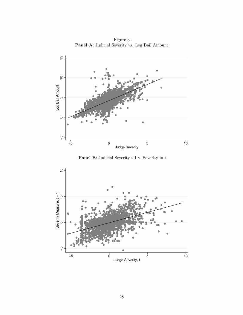
Figure 3Panel A: Judicial Severity vs. Log Bail Amount

−5

05

10

15

Log B

ail

Am

ount

−5 0 5 10Judge Severity

Panel B: Judicial Severity t-1 v. Severity in t

−5

05

10

Severity

Measure

, t −

1

−5 0 5 10Judge Severity, t

28

Table 1Summary Statistics

Philadelphia Pittsburgh

Mean SD Mean SD

Age 33.5 11.6 33.4 11.7Non-White 0.56 - 0.42 -Race Missing 0.12 - 0.027 -Male 0.81 - 0.77 -Prior Cases 0.42 - 0.33 -Total Offenses 3.42 2.95 4.68 3.48Case Guilty 0.50 - 0.77 -Total Bail 24083 74891 12964 28697Money Bail 0.62 - 0.53 -Posted Money Bail 0.31 - 0.24 -Bench Warrant 0.019 - 0.15 -Charged With Future Crime 0.43 - 0.33 -

Sample Size 203188 57145

The sample includes criminal cases in Philadelphia and Pittsburgh in the period 2010–2015. Bail information is reportedfrom the magistrate level; case disposition information is taken from the most severe offense for which the defendant wascharged; and bench warrant information is taken from a merged dataset of all bench warrants filed in association witha particular docket. Prior cases are taken within our sample, so the measure does not account for crimes committedin the period prior to our sample. Defendants are recorded as having posted money bail if money bail was initially setand their bail status was at some point listed as posted.

29

Table 2OLS Regressions of Guilt on assigned Bail

No Controls Offense FEs Full Controls Full Controls(1) (2) (3) (4)

Any Money Bail 0.014∗ 0.092∗∗∗ 0.043∗∗∗

(0.008) (0.007) (0.006)

Log(Money Bail) 0.004∗∗∗

(0.001)

Proportion Guilty 0.498 0.498 0.498 0.498N 200643 200643 200617 200617

Case Controls No No Yes YesOffense FEs No Yes Yes YesMonth FEs Yes Yes Yes Yes

OLS regressions of a binary indicator of a case disposition of guilt on a binary indicator equal to 1 ifmoney bail is initially assigned to the case (Columns 1-3) or the continuous measure log[1+money bailamount] (column 4). Case controls include age, age2, prior cases, number of offenses, and indicators forrace, gender and out-of-state.Offense and month of arraignment fixed effects are also included. Standarderrors are clustered at the judge-year level * p < 0.10, ** p < 0.05, *** p < 0.01.

30

Table 3Randomization Tests

Joint Regressions

Means Pairwise No Controls Controls(1) (2) (3) (4)

Non-White 0.56 0.00035 0.00037 0.00020(0.000) (0.001) (0.001)

Race Missing 0.12 -0.00026 -0.000015 -0.00014(0.001) (0.001) (0.001)

Male 0.81 0.00053 0.00043 -0.000066(0.001) (0.001) (0.001)

Age 33.5 -0.0000010 -0.00000041 0.000016(0.000) (0.000) (0.000)

Out of State 0.031 0.0018 0.0019 0.0026(0.001) (0.001) (0.002)

Prior Cases 0.42 0.00013 0.00013 0.00037(0.000) (0.000) (0.001)

N. of cases 200617 200617F-Statistic 0.54 0.34

Offense FEs No Yes YesMonth FEs No No Yes

OLS regressions of our judge severity measure on case characteristics for thePhiladelphia sample. Column 1 presents means of case characteristics. Column2 presents coefficients of separate bivariate regressions of the judge severity mea-sure on each case characteristic. Column 3 contains the coefficients from a singleregression of the judge severity measure on all case characteristics and month fixedeffects. Column 4 shows the coefficients from a regression identical to column 3,but additionally including offense fixed effects. F-statistics are reported for the testof joint significance of all shown case characteristics. * p < 0.10, ** p < 0.05, ***p < 0.01.

31

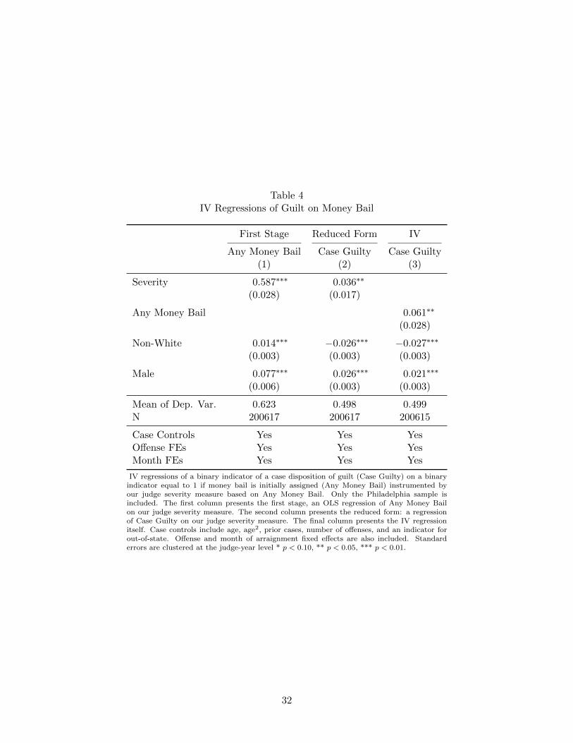
Table 4IV Regressions of Guilt on Money Bail

First Stage Reduced Form IV

Any Money Bail Case Guilty Case Guilty(1) (2) (3)

Severity 0.587∗∗∗ 0.036∗∗

(0.028) (0.017)

Any Money Bail 0.061∗∗

(0.028)

Non-White 0.014∗∗∗ −0.026∗∗∗ −0.027∗∗∗

(0.003) (0.003) (0.003)

Male 0.077∗∗∗ 0.026∗∗∗ 0.021∗∗∗

(0.006) (0.003) (0.003)

Mean of Dep. Var. 0.623 0.498 0.499N 200617 200617 200615

Case Controls Yes Yes YesOffense FEs Yes Yes YesMonth FEs Yes Yes Yes

IV regressions of a binary indicator of a case disposition of guilt (Case Guilty) on a binaryindicator equal to 1 if money bail is initially assigned (Any Money Bail) instrumented byour judge severity measure based on Any Money Bail. Only the Philadelphia sample isincluded. The first column presents the first stage, an OLS regression of Any Money Bailon our judge severity measure. The second column presents the reduced form: a regressionof Case Guilty on our judge severity measure. The final column presents the IV regressionitself. Case controls include age, age2, prior cases, number of offenses, and an indicator forout-of-state. Offense and month of arraignment fixed effects are also included. Standarderrors are clustered at the judge-year level * p < 0.10, ** p < 0.05, *** p < 0.01.

32

Table 5IV Regressions of Guilt × Detention Status on Money Bail

Guilty Not Guilty

Detained Released Detained Released(1) (2) (3) (4)

Any Money Bail 0.161∗∗∗ −0.098∗ 0.014 −0.077(0.059) (0.060) (0.050) (0.053)

Non-White −0.006∗∗ −0.021∗∗∗ 0.029∗∗∗ −0.003(0.002) (0.003) (0.003) (0.004)

Male 0.029∗∗∗ −0.008 0.028∗∗∗ −0.049∗∗∗

(0.005) (0.005) (0.006) (0.006)

Mean of Dep. Var. 0.226 0.272 0.178 0.323N 200615 200615 200615 200615

Case Controls Yes Yes Yes YesOffense FEs Yes Yes Yes YesMonth FEs Yes Yes Yes Yes

IV regressions of a binary indicator of a new measure of full defendant outcomes ona binary indicator equal to 1 if money bail is initially assigned (Any Money Bail)instrumented by our judge severity measure based on Any Money Bail. Only thePhiladelphia sample is included. Outcomes for defendants are split into four categoriescorresponding to the interaction of being detained and a case disposition of guilty.Detained defendants were either remanded without the ability to post bail, or failedto post bail given the assessment of money bail. Released individuals either did notreceive money bail or posted money bail. Each of the four columns presents an IVregression with one of those category as the dependent variable. Case controls includeage, age2, prior cases, number of offenses, and an indicator for out-of-state. Offenseand month of arraignment fixed effects are also included. Standard errors are clusteredat the judge-year level * p < 0.10, ** p < 0.05, *** p < 0.01.

33

Table 6IV Regressions of Guilt on Money Bail by Case Characteristics

Felony Public Defender Male Non-White(1) (2) (3) (4)

Any Money Bail 0.081 0.054∗ 0.060∗ 0.083∗∗

(0.061) (0.029) (0.032) (0.034)

Non-White −0.045∗∗∗ −0.026∗∗∗ −0.026∗∗∗

(0.003) (0.003) (0.003)

Male 0.020∗∗∗ 0.024∗∗∗ 0.024∗∗∗

(0.006) (0.004) (0.004)

Proportion Guilty 0.541 0.492 0.509 0.515N 94658 126757 162691 112280

Case Controls Yes Yes Yes YesOffense FEs Yes Yes Yes YesMonth FEs Yes Yes Yes Yes

IV regressions of a binary indicator of case dispositions on a binary indicator equal to 1if money bail is initially assigned (Any Money Bail) instrumented by our judge severitymeasure based on Any Money Bail. Only the Philadelphia sample is included. Each columnrestricts to the subsample indicated in the column header. Felony refers to defendants arewho are charged with a felony offenses, public defender refers to defendants represented bypublic defenders. Case controls include age, age2, prior cases, number of offenses, and anindicator for out-of-state. Offense and month of arraignment fixed effects are also included.Standard errors are clustered at the judge-year level * p < 0.10, ** p < 0.05, *** p < 0.01.

34

Table 7IV Regressions of Guilt on Log(Money Bail)

First Stage Reduced Form IV

Log(Money Bail) Case Guilty Case Guilty(1) (2) (3)

Severity 0.561∗∗∗ 0.004∗

(0.027) (0.002)

Log(Money Bail) 0.006∗∗

(0.003)

Non-White 0.153∗∗∗ −0.026∗∗∗ −0.027∗∗∗

(0.024) (0.003) (0.003)

Male 0.829∗∗∗ 0.026∗∗∗ 0.021∗∗∗

(0.058) (0.003) (0.004)

Mean of Dep. Var. 5.695 0.498 0.499N 200617 200617 200615

Case Controls Yes Yes YesOffense FEs Yes Yes YesMonth FEs Yes Yes Yes

IV regressions of a binary indicator of a case disposition of guilt (Case Guilty) on the con-tinuous measure log[1+money bail amount] (Log(Money Bail)) instrumented by our judgeseverity measure based on Log(Money Bail). Only the Philadelphia sample is included. Thefirst column presents the first stage, an OLS regression of Log(Money Bail) on our judge sever-ity measure. The second column presents the reduced form: a regression of Case Guilty onour judge severity measure. The final column presents the IV regression itself. Case controlsinclude age, age2, prior cases, number of offenses, and an indicator for out-of-state. Offenseand month of arraignment fixed effects are also included. Standard errors are clustered at thejudge-year level * p < 0.10, ** p < 0.05, *** p < 0.01.

35

Table 8IV Regressions of Guilt on Log(Money Bail) – Intensive Margin

First Stage Reduced Form IV

Log(Money Bail | Bail>0) Case Guilty Case Guilty(1) (2) (3)

Severity 0.489∗∗∗ −0.006(0.035) (0.008)

Log(Money Bail | Bail > 0) −0.013(0.016)

Non-White 0.047∗∗∗ −0.037∗∗∗ −0.036∗∗∗

(0.007) (0.002) (0.002)

Male 0.344∗∗∗ 0.019∗∗∗ 0.023∗∗∗

(0.021) (0.004) (0.006)

Mean of Dep. Var. 9.143 0.506 0.499N 124352 124352 124338

Case Controls Yes Yes YesOffense FEs Yes Yes YesMonth FEs Yes Yes Yes

IV regressions of a binary indicator of a case disposition of guilt (Case Guilty) on the continuous measure log[moneybail amount], instrumented by our judge severity measure based on log[money bail amount]. Only the Philadelphiasample is included, and defendants with no money bail are excluded. The first column presents the first stage, anOLS regression of log[money bail amount] on our judge severity measure. The second column presents the reducedform: a regression of Case Guilty on our judge severity measure. The final column presents the IV regression itself.Case controls include age, age2, prior cases, number of offenses, and an indicator for out-of-state. Offense and monthof arraignment fixed effects are also included. Standard errors are clustered at the judge-year level * p < 0.10, **p < 0.05, *** p < 0.01.

36

Table 9IV Regressions of Guilt on Money Bail – Pittsburgh

First Stage Reduced Form IV

Any Money Bail Case Guilty Case Guilty(1) (2) (3)

Severity 0.391∗∗∗ 0.025∗

(0.026) (0.013)

Any Money Bail 0.064∗∗

(0.031)

Non-White 0.107∗∗∗ −0.004 −0.011(0.006) (0.006) (0.007)

Male 0.084∗∗∗ 0.053∗∗∗ 0.047∗∗∗

(0.006) (0.006) (0.006)

Mean of Dep. Var. 0.495 0.777 0.766N 38149 38149 38141

Case Controls Yes Yes YesOffense FEs Yes Yes YesMonth FEs Yes Yes Yes

IV regressions of a binary indicator of a case disposition of guilt (Case Guilty) on a binaryindicator equal to 1 if money bail is initially assigned (Any Money Bail) instrumented by ourjudge severity measure based on Any Money Bail. Only the Allegheny county (Pittsburgh)sample is included. The first column presents the first stage, an OLS regression of AnyMoney Bail on our judge severity measure. The second column presents the reduced form:a regression of Case Guilty on our judge severity measure. The final column presents theIV regression itself. Case controls include age, age2, prior cases, number of offenses, and anindicator for out-of-state. Offense and month of arraignment fixed effects are also included.Standard errors are clustered at the office-judge-year level * p < 0.10, ** p < 0.05, ***p < 0.01.

37

Table 10IV Panel Regressions of Recidivism on Money Bail

Philadelphia Combined Sample

All Charges All Charges Felony Misdemeanor(1) (2) (3) (4)

Any Money Bail 0.007 0.007∗∗ 0.002 0.006∗∗

(0.008) (0.004) (0.003) (0.003)

Non-White −0.012∗∗∗ −0.008∗∗∗ 0.003∗∗∗ −0.012∗∗∗

(0.001) (0.001) (0.001) (0.001)

Male 0.026∗∗∗ 0.017∗∗∗ 0.018∗∗∗ 0.002∗∗∗

(0.001) (0.001) (0.001) (0.001)

Mean of Dep. Var. 0.117 0.0811 0.0442 0.0424N 522395 862163 862163 862163

Case Controls Yes Yes Yes YesOffense FEs Yes Yes Yes YesMonth of Initial Offense FEs Yes Yes Yes YesCalendar Year FEs Yes Yes Yes Yes

IV regressions of recidivism on a binary indicator equal to 1 if money bail is initially assigned (Any MoneyBail) instrumented by our judge severity measure. Recidivism is a binary indicator equal to one if the defendantis charged with a new offense in the current calendar year following the case in question. Only the IV regressionis displayed in each column. Defendants are included in a yearly panel starting with the calendar year of offenseuntil 2015 (the last year for which we have criminal charge data). Case controls are taken from the first casein our records only, and include age, age2, prior cases, number of offenses, and an indicator for out-of-state.Subsequent charges are included only as instances of recidivism. Offense and month of arraignment fixed effectsare also included, as are controls for the calendar year. The first column includes data only from Philadelphia(episodes of recidivism may reflect future crimes committed anywhere else in the state); the remaining columnsinclude combined data from Pittsburgh and Philadelphia (the “Combined Sample”). Column 3 uses as adependent variable only future crimes which are classified as felonies; column 4 focuses on future misdemeanoroffenses. Standard errors are clustered at the defendant level * p < 0.10, ** p < 0.05, *** p < 0.01.

38

Table 11IV Regressions of Failure to Appear on Money Bail

Philadelphia Combined Sample

Explicit FTA Warrant Explicit FTA Warrant(1) (2) (3) (4)

Any Money Bail 0.003 0.018 0.002 0.005(0.003) (0.021) (0.002) (0.008)

Non-White −0.000 −0.001 −0.000 −0.001(0.000) (0.001) (0.000) (0.001)

Male −0.000 −0.000 −0.000 0.000(0.000) (0.002) (0.000) (0.001)

Mean of Dep. Var. 0.001 0.010 0.001 0.007N 200615 200615 238614 299779

Case Controls Yes Yes Yes YesOffense FEs Yes Yes Yes YesMonth FEs Yes Yes Yes Yes

IV regressions of binary indicators for failing to appear (FTA) at court dates on a binary indi-cator equal to 1 if money bail is initially assigned (Any Money Bail) instrumented by our judgeseverity measure based on Any Money Bail. The two columns present two different variablesindicating that the defendant failed to appear. Calendar FTA is an indicator equal to one ifthe defendant is explicitly listed as having failed to appear at a scheduled calendar event in thedata. Bench Warrant FTA is an indicator if a bench warrant was issued for the defendant. Onlythe Philadelphia sample is included. Case controls include age, age2, prior cases, number ofoffenses, and an indicator for out-of-state. Offense and month of arraignment fixed effects arealso included. Standard errors are clustered at the judge year level * p < 0.10, ** p < 0.05, ***p < 0.01.

39

Appendix

40

Tab

leA

1:C

omm

onO

ffen

ses

Cou

nt

Any

Mon

eyB

ail

Bail

Am

ou

nt

Non

-Wh

ite

Male

Inte

nti

onal

Pos

sess

ion

ofa

Con

trol

led

Su

bst

ance

22,8

4615

%$643

48%

84%

Man

ufa

ctu

re,

Del

iver

y,or

Pos

sess

ion

Wit

hIn

tent

toM

anu

fact

ure

orD

eliv

er18

,913

87%

$17,5

11

56%

92%

Agg

rava

ted

Ass

ault

12,4

1797

%$49,6

45

63%

77%

DU

I:1s

tO

ffen

se11

,436

27%

$2,1

66

43%

82%

Ret

ail

Th

eft-

Tak

eM

erch

and

ise

10,4

2436

%$1,2

84

58%

63%

Sim

ple

Ass

ault

6,29

384

%$4,4

49

54%

80%

Pos

sess

ion

ofIn

stru

men

tO

fC

rim

eW

/Inte

nt

toE

mp

loy

6,08

185

%$10,9

28

54%

66%

Rec

eivin

gS

tole

nP

rop

erty

5,86

555

%$14,2

05

59%

85%

Pos

sess

ion

Of

Mar

iju

ana

5,64

110

%$433

72%

92%

Pu

rch

ase

orre

ceip

tof

Con

trol

led

Su

bst

ance

by

Un

auth

oriz

edP

erso

n5,

518

11%

$288

35%

76%

41

Table A2: Randomization Check in Pittsburgh

Joint Regressions

Means Pairwise No Controls Controls(1) (2) (3) (4)

Non-White 0.42 0.019∗∗∗ 0.019∗∗∗ 0.015∗∗∗

(0.002) (0.002) (0.004)Race Missing 0.027 0.0050 0.015∗∗ -0.013

(0.007) (0.007) (0.011)Male 0.77 0.014∗∗∗ 0.013∗∗∗ 0.0093∗∗∗

(0.003) (0.003) (0.003)Age 33.4 -0.00011 -0.000042 0.000053

(0.000) (0.000) (0.000)Out of State 0.029 0.015∗∗ 0.016∗∗ 0.014∗

(0.007) (0.007) (0.009)Prior Cases 0.33 -0.0063∗∗∗ -0.0060∗∗ 0.0036

(0.002) (0.002) (0.003)

N. of cases 38149 38149F-Statistic 20.0 4.74

Offense FEs No Yes YesMonth FEs No No Yes

42

Table A3: IV Specification by Bail Amounts

1st Quartile 2nd Quartile 3rd Quartile 4th Quartile(1) (2) (3) (4)

Any Money Bail 0.097∗∗ 0.013 0.068 0.040(3.05) (0.07) (0.57) (0.30)

Age 0.014∗∗ 0.0047 -0.0078∗∗ -0.0097∗∗

(10.44) (1.52) (-4.06) (-7.25)Age2 -0.00016∗∗ -0.000039 0.000084∗∗ 0.00011∗∗

(-10.29) (-1.12) (3.37) (6.03)Non-White -0.040∗∗ 0.011∗ -0.063∗∗ -0.055∗∗

(-5.82) (2.11) (-11.55) (-8.32)Race Missing -0.22∗∗ -0.16∗∗ -0.20∗∗ -0.19∗∗

(-23.65) (-8.70) (-9.96) (-13.71)Male -0.021∗∗ 0.036∗∗ 0.11∗∗ 0.033∗∗

(-3.95) (3.08) (6.86) (4.21)Offense Controls Yes Yes Yes YesOther Controls Yes Yes Yes YesOffice × Month Yes Yes Yes Yes

N. of cases 43974 47396 46327 46047Avg. Bail Amount 734.2 3638.5 14974.9 65859.3

Marginal effects; t statistics in parentheses

(d) for discrete change of dummy variable from 0 to 1∗ p < 0.05, ∗∗ p < 0.01

43

Table A4: IV Specification by Bail Amounts, Extensive Margin

IV Coefficient N Avg. Bail(1) (2) (3)

Panel A: FeloniesDrug Possession, Distribute 0.016 23652 16940.5

(0.27)Aggravated Assault -0.33∗ 12382 49633.7

(-2.36)Burglary -0.086 4420 20715.6

(-0.43)Retail Theft 0.24∗ 4323 2075.2

(2.59)Receiving Stolen Property 0.21∗ 3644 20077.5

(2.38)Panel B: Misdemeanors

Possession of Drugs 0.023 22776 542.1(0.62)

1st DUI 0.024 11419 2166.3(0.56)

Simple Assault 0.048 6270 4449.4(0.71)

Gun Possession 0.019 6064 10927.9(0.20)

Retail Theft 0.11∗ 6059 719.6(2.03)

Offense Controls Yes Yes YesOther Controls Yes Yes YesOffice × Month Yes Yes Yes

Marginal effects; t statistics in parentheses

(d) for discrete change of dummy variable from 0 to 1∗ p < 0.05, ∗∗ p < 0.01

44

Table A5: IV Specification by Bail Amounts, Intensive Margin

IV Coefficient N Avg. Bail(1) (2) (3)

Panel A: FeloniesDrug Possession, Distribute -0.016 20336 16940.5

(-0.98)Aggravated Assault -0.020 12033 49633.7

(-0.62)Burglary 0.046 4185 20715.6

(1.27)Retail Theft 0.059 2318 2075.2

(1.01)Receiving Stolen Property -0.39 2078 20077.5

(-0.83)Panel B: Misdemeanors

Possession of Drugs -0.100∗∗ 3412 542.1(-2.90)

1st DUI -0.021 3090 2166.3(-0.55)

Simple Assault -0.022 5239 4449.4(-0.67)

Gun Possession 0.096∗∗ 5147 10927.9(2.84)

Retail Theft -0.027 1442 719.6(-0.68)

Offense Controls Yes Yes YesOther Controls Yes Yes YesOffice × Month Yes Yes Yes

Marginal effects; t statistics in parentheses

(d) for discrete change of dummy variable from 0 to 1∗ p < 0.05, ∗∗ p < 0.01

45