The Haar Wavelet Transform of a Dendrogram:

Additional Notes

Fionn Murtagh∗

June 14, 2006

Abstract

We consider the wavelet transform of a finite, rooted, node-ranked,p-way tree, focusing on the case of binary (p = 2) trees. We studya Haar wavelet transform on this tree. Wavelet transforms allow formultiresolution analysis through translation and dilation of a waveletfunction. We explore how this works in our tree context.

Keywords: Haar wavelet transform; binary tree; ultrametric topology; p-adic numbers; hierarchical clustering; data mining; local field; abelian group.

1 Introduction

In a companion paper, which we will refer to as Paper I (“The Haar wavelettransform of a dendrogram”), a new transform is applied to a hierarchicalclustering. Various examples are given of uses of this transform, prior toapplying the inverse transform.

In this paper, we look at linkages with other ways of understanding thewavelet transform, with the classical demarche described in Appendix 1.Our aim is to understand the wavelet transform when applied to hierarchi-cal clustering dendrograms (where notation and expression as ultrametrictopology are summarized in Appendix 2).

After all, both the wavelet transform and hiearchical clustering aspireto multiresolution or multiscale analysis. The natural question is then: howdo they differ and are there different aspects that they bring to the dataanalysis task?

∗F. Murtagh is with the Department of Computer Science, Royal Holloway, University

of London, Egham, Surrey, TW20 0EX, England. Email fmurtagh@acm.org

1

A good deal of recent work on wavelet transform has been through grouptheoretic approaches.

Foote et al. (2000a) point to how group theoretic understanding canlead to a “wealth of new analysis filters” (in the context of multiresolu-tion signal and image analysis). The same point is made by the SMARTproject (SMART, 2005), including the change to have automatic generationof new transform algorithms. Believing that algorithms should be developedif and only if the there is a verifiable user need for them, we would insteadpoint to another reason why group theoretic understanding is crucial to dataanalysis. A great deal of observed reality can be understood by way of ob-served symmetries, and groups summarized and encapsulate the propertiesof these symmetries. For time evolving phenomena, therefore, or spatial co-ordinate referenced phenomena, it may be possible to replace analysis that istime-referenced or referenced to particular coordinate systems with a moregeneral, more generic, symmetry analysis. This is the vision opened up bythe study of group actions on a set of objects.

Parenthically, one fascinating way as to how this works can be seen inCendra and Marsden (2003). The authors develop (i) an analytic theory ofdynamics as functions of spatial and temporal coordinates; and (ii) grouptheoretic interpretation of, in parts of the study, return or phase maps.

Our approach can be stated as follows. Let U be an ultrametric space,associated with an m-dimensional embedding, Rm. We note that an ultra-metric space is necessarily of 0 dimenensionality; and that minimal dimen-sionality real embedding of an ultrametric has been studied by Lemin andothers (Lemin, 2001; Bartal et al., 2004).

The partial order of (clopen) set inclusion is denoted by the binary treeor hierarchy, H. Consider the group action comprising rotations or cyclicpermutations (these are equivalent) of subnodes of any node in H, and wewill denote this group as GH . Then we study the wavelet transform of L2(U)resulting from the actions of group GH .

Having already discussed the new wavelet transform in Paper I, we cangive one result relating to it in the context of the group of equivalent repre-sentations of H as follows.

Theorem: For all 2n−1 equivalent representations of H (here: unlabeledgraph isomorphisms), the dendrogram Haar wavelet transform is unique.

The proof follows from the definition of the wavelet coefficents at eachlevel, ν; whereas the equivalent representations of H are intra level.

It follows from this theorem that we have a unique matrix representationof a dendrogram.

2

2 Previous Work on Wavelet Transforms of Data

Tables

In this section we will review recent work using wavelet transforms on datatables, and show how our work represents a radically new approach to tack-ling similar objectives.

Approximate query processing arises when data must be kept confiden-tial so that only aggregate or macro-level data can be divulged. Approxi-mate query processing also provides a solution to access of information frommassive data tables.

One approach to approximate database querying through aggregates issampling. However a join operation applied to two uniform random samplesresults in a non-uniform result, which furthermore is sparse (Chakrabarti,Garofalakis, Rastogi and Shim, 2001). A second approach is to keep his-tograms on the coordinates. For a multidimensional feature space, one isfaced with a “curse of dimensionality” as the dimensionality grows. A thirdapproach is wavelet-based, and is of interest to us in this article.

A form of progressive access to the data is sought, such that aggregateddata can be obtained first, followed by greater refinement of the data. TheHaar wavelet transform is a favored transform for such purposes, given thatreconstructed data at a given resolution level is simply a recursively definedmean of data values. Vitter and Wang (1999) consider the combinatorialaspects of data access using a Haar wavelet transform, and based on a multi-way data hypercube. Such data, containing scores or frequencies, is oftenfound in the commercial data mining context of OLAP, On-Line AnalyticalProcessing.

As pointed out in Chakrabarti et al. (2001), one can treat multidimen-sional feature hypercubes as a type of high dimensional image, taking thegiven order of feature dimensions as fixed. As an alternative a uniform “shiftand distribute” randomization can be used (Chakrabarti et al., 2001).

There are problems, however, in directly applying a wavelet transformto a data table. Essentially, a relational table (to use database terminology;or matrix) is treated in the same way as a 2-dimensional pixelated image,although the former case is invariant under row and column permutation,whereas the latter case is not (Murtagh, Starck and Berry, 2000). Thereforethere are immediate problems related to non-uniqueness, and data orderdependence.

What if, however, one organizes the data such that adjacency has a mean-ing? This implies that similarly-valued objects, and/or similarly-valued fea-

3

tures, are close together. This is what we do, using any hierarchical cluster-ing algorithm (e.g., the Ward or minimum variance one).

Without loss of generality, as seen in these figures, we assume that ahierarchy is a binary, rooted tree; and equivalently that the series of ag-glomerations involve precisely two clusters (possibly singleton clusters) ateach of the n − 1 agglomerations where there are n observations. These nobservations are usually represented by n row vectors in our data table.

A significant advantage in regard to hierarchical clustering is that parti-tions of the data can be read off at a succession of levels, and this obviatesthe need for fixing the number of clusters in advance. All possible clusteringoutcomes are considered. (Remark: of course, relative to any one of thecommonly used cluster homogeneity criteria, each partition is guaranteed tobe sub-optimal at best.)

3 The Haar Wavelet Transform of a Dendrogram:

Summary

In this article, we will denote the agglomeration of two clusters, q and q′, ascluster q′′. So (left or right subtree) nodes in the dendrogram are associatedwith the child (elder or younger) subnodes. We can define the elder clusteras q such that ν(q) > ν(q′), but we will not be concerned with whether ornot elder corresponds to left, and younger to right.

For n objects or observation vectors, another notation that we can useis that the hierarchy H is the set of clusters indexed from 1 to n: H ={q1, q2, . . . , qn−1}. We will always assume in this article, for convenience ofexposition and with little loss of generality, that for distinct clusters ν(q) 6=ν(q′).

Whenever the distinction between the following become important, wewill clearly distinguish between them: clusters; nodes; sets of objects; setsof indices of objects; and p-adic number representation of indices of objects.

The Haar algorithm, as discussed in Paper I, is as follows:

1. Take each cluster q′′ in turn, proceeding in sequence through q′′ ∈{q1, q2, . . . , qn−1}.

2. Apply the smoothing function, s: s(q′′) = 12(q + q′).

3. Thereby apply the detail function, d: d(q′′) = s(q′′)−s(q′) = −(s(q′′)−s(q)).

4. Return to step 1 until all n− 1 clusters are processed.

4

For details of how the clusters also take terminal nodes (objects) intoaccount, see Paper I.

Now, it is clear from construction that perfect reconstruction of theinput data (alternatively expressed, perfect undoing of the foregoing Haaralgorithm) is guaranteed, given all of the following: (i) all of the detailfunction values, (ii) the final smooth, s(qn−1), (iii) the definition of thedendrogram, and (iii) a convention of left and right subtree that allows usto traverse down the tree from q′′ to both q and q′.

In practice our objectives are to explore the foundations of two distinctapproaches. Both seek a Haar wavelet basis. These two approaches areas follows and can express the 2 input data cases considered in section 4.3(“The Input Data”) of Paper I.

• Wavelet transform in an ultrametic topology: Induce the Haar ba-sis from the hierarchy H that expresses the relationships in a set ofultrametrically related points, I.

• Wavelet transform on embedded subsets: Induce the Haar basis fromthe hierarchy H defining a set of subsets of I.

In the ultrametric case, each point i ∈ I defines anm-dimensional vector:i ∈ Rm. For notational convenience therefore i is either the index, or avector.

In the set of subsets case, each point i ∈ I can be defined as an n-dimensional index vector. Thus for example the sequentially second pointis defined as (0, 1, 0, 0, . . . , 0).

Both practical cases above can be expressed as follows: we carry out awavelet transform in L2(G) where G is the group of alternative representa-tions of a given hierarchy, H. The points i ∈ I are associated either withvectors in Rm or with an orthonormal vector set in Zn. (Note how Zn isn-dimensional, whereas Rm is m-dimensional. The cardinality of I is n. Thedimensionality of a feature or attribute space is m.)

4 Wavelet Transform on Discrete Fields

In this section we look at the wavelet transform on discrete fields, and inparticular on ℓ2(Zp). This is realized through cyclic representations of theaffine group of Z or of Zp.

In wavelets, we are seeking a representation of our data which has “co-variant” properties relative to scale: for example, for tranlation “covari-ance”, the representation of a shifted signal must be a shifted copy of the

5

representation of the signal (Torresani, 1994). In the group theory per-spective, such “covariance” properties (i.e. with respect to the action of asymmetry group) are the starting point, and the representation is to be de-rived from them. The “covariance” group “turns out to be isomorphic (upto a compact factor) to the geometric phase space of the representation”(Torresani, 1994, p. 6).

Traditionally, the wavelet transform is covariant with respect to a groupaction applicable to images, signals, time series, etc., viz. the affine groupof the real line, which is a continuous group (Antoine et al., 2000a). Thus afirst task is to bypass the need for a continuous group.

The group law of the affine group, in generic form ax + b, generatestranslations and dilations. The action of the ax + b group on R means:(a, b) : x −→ ax+ b. We have the following product:

(b, a) · (b′, a′) = (b+ ab′, aa′) (1)

Here, the identity is: (1, 0). The inverse of (a, b) is: (a, b)−1 = (a−1,− ba).

This is a non-commutative Lie (and thus continuous) group.Flornes et al. (1994) consider a discrete wavelet transform to begin with,

specified on the Hilbert space ℓ2(Zp) (where Z are the integers, Zp are in-tegers mod p where p is prime for reasons explained below; and ℓ2 impliesfinite energy from discrete values, or being square integrable). The Haarmeasure is defined on locally compact groups, permitting integration overgroup actions or members; and a locally compact separable group is con-sistent with the square integrable property. The group at issue here is thecyclic representation of the affine group; or its finite analog, the affine groupmod p (Foote et al., 2000a).

A discussion of square integrable group representations in the context oftime-frequency transforms, including the continuous wavelet transform, canbe found in Torresani (2000); and Torresani (1994) discusses the counterex-ample case of the rotation group, S2, on the 2-dimensional sphere, whichgives rise to a representation which is not square integrable.

The wavelet transform considered by Flornes et al. (1994) has the fol-lowing operations:

Translation : Tbf(n) = f(n− b) for f ∈ ℓ2(Zp) (2)

Dilation : Daf(n) = f(a−1n)

(3)

6

The reason why p has to be prime is as follows. Consider the p-adicnumber representation of Zp. For the p-adic respresentation of Zp to be afield, i.e. to have an inverse, p must be prime.

The unitary representation of a group G is a mapping into a (complex)Hilbert space. Flornes et al. (1994) define the following unitary representa-tion, π, on the group, mapping into unitary operations on ℓ2(Zp):

π(g)f(n) = f(a−1(n− b))

In terms of the translation and dilation operators, we have:

π(b, a) = TbDa

Thus far, a purely discrete wavelet transform is at issue. However if wetake our function values f defined on Zp as sampled values from a continuoussignal, then problems of interpolation arise. It simply is not good enoughto transform our discrete data independently of awareness of the underlyingcontinuum. Note that this issue is at the nub of where data analysis differsfrom signal processing. In data analysis, mostly a data cloud is taken asgiven (potentially leading to a combinatorial perspective) or as a stochasticrealization (leading to a statistical modeling). In signal processing, theobserved data are samples of an underlying topological or other continuousstructure. It is a prime objective in the signal processing context to keepthe processing of the observed, sampled data fully and provably consistentwith the underlying continuous structures.

A way to address this issue of interpolation is to use B spline filters (thesimplest example of which is the box function used by the Haar wavelettransform) to smooth the data, thereby “filling the holes” between gaps inthe sampled values, before dilating. This is termed pseudo-dilation.

Relations (3) can be re-expressed as follows (Torresani, 1994):

Translation : Tbf(n) = f(n− b) for f ∈ ℓ2(Zp) (4)

Dilation : Daf(n) = f(a−1n) if a divides n

= 0 otherwise

(5)

Then the affine multiplication law is verified by {Tb, Da} (using relation1):

TbDaTb′Da′ = Tb+ab′Daa′ (6)

7

When f ∈ ℓ2(Zp) with p prime, then a always divides n. The affinegroup on ℓ2(Zp) is well-defined; Tb and Da define a representation of thisgroup; and it turns out that the square integrable property holds.

In general for f ∈ ℓ2(Z) the a trous algorithm is used incorporating bothcontinuously defined dilation, and discretization of the function.

We could embed each node of a hierarchical clustering, defined as wealways do so as binary, rooted tree, in Z2. Lang (1998) develops a wavelettransform approach (including the Haar wavelet transform and others) forsuch a 2-series local field, or Cantor dyadic group. Taking each cluster q ∈ Qor node in the tree individually is not satisfactory from our point of view,and so we look further for a more pleasing way to process a hierarchy.

5 Wavelet Bases on Local Fields

Wavelet transform analysis is the determining of a “useful” basis for L2(Rm)with the following properties:

• induced from a discrete subgroup of Rm,

• using translations on this subgroup, and

• dilations of the basis functions.

Classically (Frazier, 1999; Debnath and Mikusinski, 1999; Strang andNguyen, 1996) the wavelet transform avails of a wavelet function ψ(x) ∈L2(R), where the latter is the space of all square integrable functions.Wavelet transforms are bases on L2(Rm), and the discrete lattice subgroupZm is used to allow discrete groups of dilated translation operators to beinduced on Rm. Discrete lattice subgroups are typical of 2D images (thelattice is a pixelated grid) or 3D images (the lattice is the voxelated grid)or spectra or time series (the lattice is the set of time steps, or wavelengthsteps).

Sometimes it is appropriate to consider the construction of wavelet baseson L2(G) where G is some group other than R. In Foote, Mirchandani,Rockmore, Healy and Olson (2000a, 2000b; see also Foote, 2005) this isdone for the group defined by a quadtree, in turn derived from a 2D image.To consider the wavelet transform approach not in a Hilbert space but ratherin locally-defined and discrete spaces we have to change the specification ofa wavelet function in L2(R) and instead use L2(G).

Benedetto (2004) and Benedetto and Benedetto (2004) considered in de-tail the groupG as a locally compact abelian group. Analogous to the integer

8

grid, Zm, a compact subgroup is used to allow a discrete group of operatorsto be defined on L2(G). The property of locally compact (essentially: finiteand free of edges) abelian (viz., commutative) groups that is most impor-tant is the existence of the Haar measure (Ward, 1994). The Haar measureallows integration, and definition of a topology on the algebraic structure ofthe group.

Benedetto (2004) considers the following cases, among others, of waveletbases constructed via a sub-structure:

• Wavelet basis on L2(Rm) using translation operators defined on thediscrete lattice, Zm. This is the situation discussed above, which holdsfor image processing, signal processing, most time series analysis (i.e.,with equal length time steps), spectral signal processing, and so on. Aspointed out by Foote (2005), this framework allows the multiresolutionanalysis in L2(Rm) to be generalized to Lp(Rm) for Minkowski metricLp other than Euclidean L2.

• Wavelet basis on L2(Qp), where Qp is the p-adic field, using a discreteset of translation operators. This case has been studied by Kozyref,2002, 2004; Altaisky, 2004, 2005. See also the interesting overview ofKhrennikov and Kozyref (2006).

• Wavelet basis on L2(Qp) using translation operators defined on thecompact, open subgroup Zp. (It is interesting to note that Zm isdiscrete; and that the quotient Rm/Zm is compact. In contrast tothis, Zp is compact; and the quotient Qp/Zp is discrete.)

• Discussed is a wavelet basis on L2(G), for a group G, using translationoperators defined on a discrete subgroup, or discrete lattice.

• Finally the central theme of Benedetto (2004) is a wavelet basis onL2(G) where G is a locally compact abelian group, using translationoperators defined on a compact open subgroup (or operators that canbe used as such on a compact open subgroup); and with definition ofan expansive automorphism replacing the traditional use of dilation.

A motivation for the work of Benedetto (2004) and Benedetto and Benedetto(2004) is laying the groundwork for the wavelet transform on the adelic num-bers (see Appendix 3). In this work we are content to be less ambitious inregard to number systems – below we focus on a particular p-adic encodingof dendrograms; and we are also less ambitious in regard to wavelet functions

9

– staying resolutely with the Haar wavelet in this work. Our motivation isdue to our application drivers.

Locally compact abelian groups (LCAG) are a way to take Fourier anal-ysis (hence a particularly important class of harmonic analysis because soversatile) into more general settings than e.g. the reals (although the realsalso form a non-compact, but locally compact, abelian group).

The duals of members of a locally compact abelian group, defined asunitary multiplicative characters, x −→ e−2πix, also form a locally compactabelian group (Knapp, 1996). The duality pairing G and G allows for anisometry between L2(G) and L2(G) (Antoine et al., 2000).

Fourier analysis is the study of real square integrable functions that areinvariant under the group of integer translations (see Foote et al., 2000a),while abstract harmonic analysis is the study of functions on more generaltopological groups that are invariant under a (closed) subgroup.

It is interesting to compare some global properties of our approach rela-tive to the Fourier transform approach applied to decision trees in Karguptaand Park (2004). The Fourier transform lends itself well to a frequency spec-trum analysis of binary decision vectors, and the latter can be of importancefor supervised classification. On the other hand, our work makes use of bi-nary trees but in the framework of unsupervised classification. The wavelettransform shares with the Fourier transform the property that frequencyspectral information is determined from the data; and the wavelet trans-form additionally determines spatial or resolution scale information fromthe data. We have found the wavelet transform, as described in this article,to be appropriate for the type of input data that we have considered. Ingeneral terms, both we in this work, and Kargupta and Park (2004), haveas objectives the filtering and compression of data.

We need affine group action for the wavelet transform, and we have seenabove (section 4, “Wavelet transform on discrete fields”) that Zp affords usthis; but for an arbitrary discrete field, and for an arbitrary locally compactabelian group, it is tricky to find an affine group. Taking further the Florneset al. (1994) work, Antoine et al. (2000) consider an infinite locally compactabelian group, G; the restriction of G to a lattice Γ ⊂ G; A, an abeliansemigroup; and the actions of A on ℓ2(Γ). Based on a pseudodilation (i.e.,the product of a natural dilation by a convolution operator) the case of acontinuous underlying signal is studied, i.e. the relation between the semi-group acting on ℓ2(Γ), and a continuous affine group acting on L2(R). Splinefunctions are again among the wavelet functions used (among which is theHaar wavelet function associated with the B-spline of order 1).

10

The aspect of greatest interest to us here in the approach of Benedetto(2004), and Benedetto and Benedetto (2004), is to define wavelets on L2(G),with G taken as the p-adic rationals, Qp, and with the p-adic integers, Zp,on which we define translation-like operators. Firstly, we are using thereforeL2(Qp), i.e. functions defined on the rationals. Secondly, we use a discretegroup of operators on L2(Qp) which are not in themselves translation oper-ators, but may be used in an analogous way. The “trick” used is that thequotient Qp/Zp is discrete, and this will furnish the translation operators.An expansive automorphism is also needed in this context, i.e. what we usein analogy with dilation.

A number of alternatives for the subset of Qp/Zp (more strictly thequotient of the group dual by the annhilator in the dual of the compact opensubgroup) are discussed by Benedetto (2000a). Given our application-driveninterest, we will not pursue them further here. What we will do, however, isto look at how the group-based approach of Benedetto (2000a), that for themost part assumes infinite sets, can be tailored for our algorithmic – hencefinite – purposes.

We will therefore look at how we can suitably encode any given dendro-gram in terms of Qp – or indeed, as will be seen, in terms of Zp.

Next we will move on to look at how a lattice-proxy is defined on ourencoding, and thereby translation operators.

Finally, we will look at how an expansive automorphism can be replacedby expansive mapping in the finite and discrete case.

In all of this, we follow the methodology described by Benedetto (2000a);but we restrict all aspects to the finite, discrete context.

5.1 The Wreath Product Group Corresponding to a Hierar-chical Clustering

For the group actions, with respect to which we will seek invariance, we con-sider independent cyclic shifts of the subnodes of a given node (hence, at eachlevel). Equivalently these actions are adjancency preserving permutationsof subnodes of a given node (i.e., for given q, the permutations of {q′, q′′}.Due to the binary tree, or strictly pairwise agglomerations represented bythe hierarchy, the “adjacency” property is trivial. We have therefore cyclicgroup actions at each node, where the cyclic group is of order 2.

The symmetries of H are given by structured permutations of the ter-minals. The terminals will be denoted here by Term H. The full group ofsymmetries is summarized by the following algorithm:

11

1. For level l = n− 1 down to 1 do:

2. Selected node, ν ←− node at level l.

3. And permute subnodes of ν.

Subnode ν is the root of subtree Hν . We denote Hn−1 simply by H. Fora subnode ν ′ undergoing a relocation action in step 3, the internal structureof subtree Hν′ is not altered.

The algorithm described defines the automorphism group which is awreath product of the symmetric group. Denote the permutation at level νby Pν . Then the automorphism group is given by:

G = Pn−1 wr Pn−2 wr . . . wr P2 wr P1

where wr denotes the wreath product.Call Term Hν the terminals that descend from the node at level ν. So

these are the terminals of the subtree Hν with its root node at level ν. Wecan alternatively call Term Hν the cluster associated with level ν.

We will now look at shift invariance under the group action. Thisamounts to the requirement for a constant function defined on Term Hν ,∀ν.A convenient way to do this is to define such a function on the set Term Hν

via the root node alone, ν. By definition then we have a constant functionon the set Term Hν .

Let us call Vν a space of functions that are constant on TermHν . Possiblebases of Vν that were considered in Paper I are:

1. Basis vector with |TermHν | components, with 0 values except for value1 for component i.

2. Set (of cardinality n = |TermHν |) of m-dimensional observation vec-tors.

The constant function maps

L(TermH) −→ Vν

where L is the space of complex valued functions on the set Term H.Now we consider the resolution scheme arising from moving from

{TermHν′ ,TermHν′′} to TermHν . From the hierarchical clustering point ofview it is clear what this represents: simply, an agglomeration of two clusterscalled Term Hν′ and Term Hν′′ , replacing them with a new cluster, TermHν .

12

Let the spaces of constant functions corresponding to the two clusteragglomerands be denoted Vν′ and Vν′′ . These two clusters are disjoint ini-tially, which motivates us taking the two spaces as a couple: (Vν′ , Vν′′). Inthe same way, let the space of constant functions corresponding to node νbe denoted Vν .

The multiresolution scheme uses a space of zero mean denoted Wν′ν′′

with mean defined on the couple of spaces, (Vν′ , Vν′′):

Vν = (Vν′ , Vν′′)⊕Wν′ν′′ = (Vν′ ⊕Wν′ν′′ , Vν′′ ⊕Wν′ν′′)

In considering spaces of constant functions, Vν′ and Vν′′ , we know thatthe support of these spaces are, respectively, Term H ′

ν and Term Hν′′ . Soif, instead of the space of zero mean denoted Wν′ν′′ where mean is definedon the couple of spaces, (Vν′ , Vν′′), we considered the mean of the combinedsupport, Term H ′

ν∪ Term Hν′′ , then the result would be quite different. Wewould, in fact, have a cluster-weighted mean value.

5.2 Example

Let us exemplify a case that satisfies all that has been defined in the contextof the wreath product invariance that we are targeting. It also exemplifiesthe algorithm discussed in depth in Paper I. Take the constant function onVν′ to be fν′ . Take the constant function on Vν′′ to be fν′′ . Then definethe constant function on Vν to be (fν′ + fν′′)/2. Next define the zero meanfunction on Wν′ν′′ to be:

wν′ = (fν′ + fν′′)/2− fν′

in the support interval of Vν′ , i.e. Term Hν′ , and

wν′′ = (fν′ + fν′′)/2− fν′′

in the support interval of Vν′′ , i.e. Term Hν′′ .Evidently wν′ = −wν′′ .

5.3 Inverse Transform

Following on from the previous subsection, a demonstration that the algo-rithm allows for exact reconstruction of the data – the inverse transform –is as follows. The constant function on Term H corresponding to the rootnode is fn−1. The two subnodes of the root node, at levels ν ′ and ν ′′, arereconstructed from fn−1±wν′ (and, as we have seen, we can either use wν′ or

13

wν′′). We next look at the subtrees whose roots are given by the nodes (justconsidered) at levels ν ′ and ν ′′, and these subtrees are necessarily disjoint.All subnodes of these currently selected nodes are reconstructed using thesame algorithm. This procedure is iteratively continued until the terminalshave been dealt with.

5.4 Link with Agglomerative Hierarchical Clustering Algo-rithms

Comparison with traditional clustering criteria is considered next. It is clearwhy agglomerative levels are very problematic if used for choosing a goodpartition in a hierarchical clustering tree: they increase with agglomeration,simply because the cluster centers are getting more and more spread out asthe sequence of agglomerations proceeds. Directly using these agglomerativelevels has been a way to derive a partition for a very long time. An earlyreference is Mojena (1977). To see how the wavelet transform used by usleads to a very different outcome, see Paper I, where we describe use of thenorms of the wν′ vectors.

When we consider agglomerative hierarchical clustering algorithms it isclear that (i) clusters are often defined in terms of center of gravity, ormean; and (ii) this allows for defining a (vector) difference term between acluster and its immediate sub-clusters. It is also clear that the Haar waveletalgorithm is close to the method known as median or Gower’s or WPGMC– weighted pair group method using centroids: see table, p. 68, of Murtagh(1985).

We could also cater for other agglomerative criteria, subject to storingthe cluster cardinality values, and develop an algorithm that is close to theHaar wavelet one. Constant functions on spaces Vν′ and Vν′′ remain just asbefore. The zero mean functions on space Wν′ν′′ would now be generalizedto weight mean (with weights given by cluster cardinalities). Viewed in thislight, our work has led us to develop a new storage structure for hierarchicalclustering trees, which is particularly beneficial for data filtering objectives.

The novelty of our work resides in two areas: (i) we have shown theclose association between two classes of multiple resolution data analysisapproaches, agglomerative hierarchical clustering algorithms and the wavelettransform; and (ii) our motivation is not at all to construct hierarchicalclusterings in a new way but rather to illuminate further inherent ultrametricproperties of data (cf. Murtagh, 2004).

14

6 An Algebraic Representation of a Hierarchy

6.1 Introduction

The dendrogram wavelet transform has been seen to be a set of applicationsof a function applied to set members, or cluster members, associated withnodes of the hierarchy H. The non-singleton clusters comprise the set Q ={q1, q2, . . . , qn−1}. The wavelet function is applied in turn to q1, q2, . . .. Inthis paper, we are using the Haar wavelet function. But we could well useothers (e.g., Altaisky, 2004, uses the Morlet wavelet).

With each q ∈ Q there is an associated level function, ν : q −→ R+,which induces a total order on Q. We will show that the application of thewavelet function to this sequence of clusters is “dilatary” or “expansive” intwo different ways.

We will return to what these two different ways are in a moment. Thehierarchy Hν=0 contains an inceasingly embedded sequence of subsets (cor-responding to increasingly pruning the branches of the tree; Bouchki, 1996).We have: Hν=0 ⊃ Hν1 ⊃ Hν2 ⊃ . . . ⊃ Hν(n−1). Define Term as theset of terminal nodes of a hierarchy, and Card the cardinality of a set.Then Term(Hν=0) = I with Card(I) = n. Card(Term(Hν1)) = n − 1.Card(Term(Hν2)) = n− 2. . . . Card(Term(Hν(n−1))) = 1. Each applicationof the wavelet function is to the minimal (non-singleton) cluster (again seeBouchki, 1996) in each νk. Below, we will see how we promote all q ∈ Hνk

to the corresponding q ∈ Hν(k+1) by multiplying clusters (in a particularalgebraic representation) by 1/p, which is of norm p.

The “dilatory” or “expansive” character of our sequence of operations,viz., application of the wavelet function, comes from (i) the sequence ofembedded subsets of H – so we still operate on a cluster, but the data onwhich we work becomes smaller; or (ii) the sequence of levels at which wework is derived from repeatedly taking the product with 1/p of norm p.

In order to introduce this product with 1/p of norm p we first describethe p-adic algebraic representation of the hierarchy. In this representation,clusters including singletons, have an operator, denoted ⊕. This operatorallows clusters to be defined. Next, we have a null element in Q in thisalgebraic representation, and a norm of each q ∈ Q. Hence for q′, q′′ ∈ Q,we can define q′ ⊕ q′′. We have: ∃q ∈ Q s.t. q = 0. Finally, ∀q ∈ Q we have‖q‖.

15

6.2 H Expressed p-Adically: p-Adic Encoding of a Dendro-gram

We will introduce now the one-to-one mapping of clusters (including single-tons) in H into a set of p-adically expressed integers (a fortiori, rationals,Qp). The field of p-adic numbers is the most important example of ul-trametric spaces. Addition and multiplication of p-adic integers, Zp, arewell-defined. Inverses exist and no zero-divisors exist.

A terminal-to-root traversal in a dendrogram or binary rooted tree isdefined as follows. We use the path x ⊂ q ⊂ q′ ⊂ q′′ ⊂ . . . qn−1, where x is agiven object specifying a given terminal, and q, q′, q′′, . . . are the embeddedclasses along this path, specifying nodes in the dendrogram. The root nodeis specified by the class qn−1 comprising all objects.

A terminal-to-root traversal is the shortest path between the given ter-minal node and the root node, assuming we preclude repeated traversal(backtrack) of the same path between any two nodes.

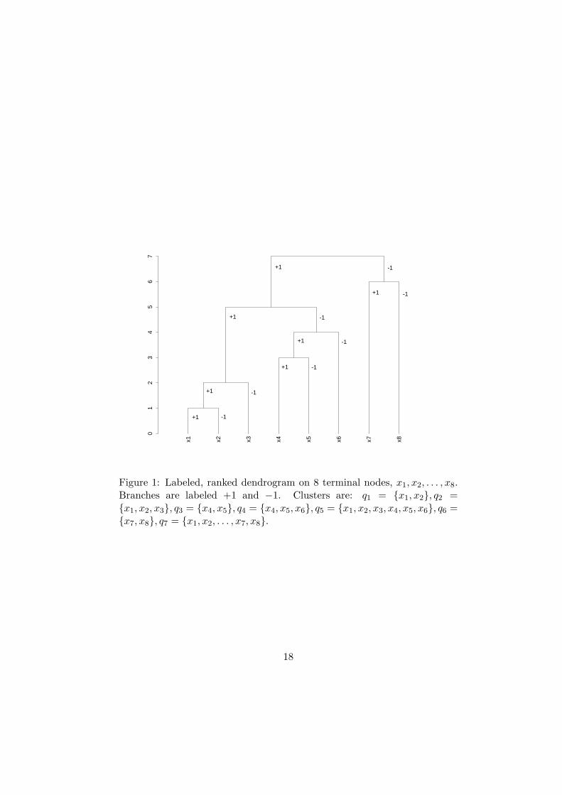
By means of terminal-to-root traversals, we define the following p-adicencoding of terminal nodes, and hence objects, in Figure 1.

x1 : +1 · p1 + 1 · p2 + 1 · p5 + 1 · p7

x2 : −1 · p1 + 1 · p2 + 1 · p5 + 1 · p7

x3 : −1 · p2 + 1 · p5 + 1 · p7

x4 : +1 · p3 + 1 · p4 − 1 · p5 + 1 · p7

x5 : −1 · p3 + 1 · p4 − 1 · p5 + 1 · p7

x6 : −1 · p4 − 1 · p5 + 1 · p7

x7 : +1 · p6 − 1 · p7

x8 : −1 · p6 − 1 · p7

If we choose p = 2 the resulting decimal equivalents could be identical:cf. contributions based on +1·p1 and −1·p1+1·p2. Given that the coefficientsof the pj terms (1 ≤ j ≤ 7) are in the set {−1, 0,+1} (implying for x1 theadditional terms: +0 · p3 + 0 · p4 + 0 · p6), the coding based on p = 3 isrequired to avoid ambiguity among decimal equivalents.

A few general remarks on this encoding follow. For the labeled rankedbinary trees that we are considering, we require the labels +1 and −1 forthe two branches at any node. Of course we could interchange these labels,and have these +1 and −1 labels reversed at any node. By doing so we willhave different p-adic codes for the objects, xi.

16

The following properties hold: (i) Unique encoding: the decimal codesfor each xi (lexicographically ordered) are unique for p ≥ 3; and (ii) Re-

versibility: the dendrogram can be uniquely reconstructed from any suchset of unique codes.

The p-adic encoding defined for any object set above can be expressedas follows for any object x associated with a terminal node:

x =

n−1∑

j=1

cjpj where cj ∈ {−1, 0,+1} (7)

In greater detail we have:

xi =n−1∑

j=1

cijpj where cij ∈ {−1, 0,+1} (8)

Here j is the level or rank (root: n− 1; terminal: 1), and i is an objectindex.

In our examples we have used: aj = +1 for a left branch (in the senseof Figure 1), = −1 for a right branch, and = 0 when the node is not on thepath from that particular terminal to the root.

A matrix form of this encoding is as follows, where {·}t denotes thetranspose of the vector.

Let x be the column vector {x1 x2 . . . xn}t.

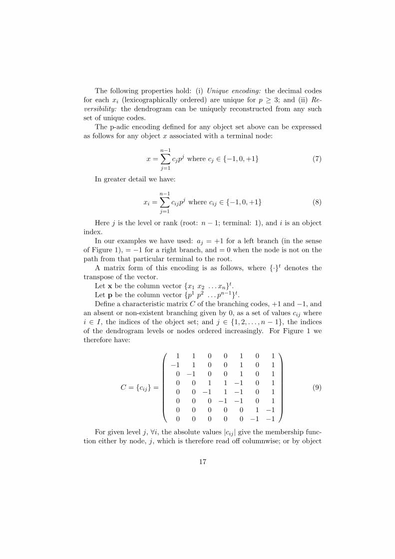
Let p be the column vector {p1 p2 . . . pn−1}t.Define a characteristic matrix C of the branching codes, +1 and −1, and

an absent or non-existent branching given by 0, as a set of values cij wherei ∈ I, the indices of the object set; and j ∈ {1, 2, . . . , n − 1}, the indicesof the dendrogram levels or nodes ordered increasingly. For Figure 1 wetherefore have:

C = {cij} =

1 1 0 0 1 0 1−1 1 0 0 1 0 1

0 −1 0 0 1 0 10 0 1 1 −1 0 10 0 −1 1 −1 0 10 0 0 −1 −1 0 10 0 0 0 0 1 −10 0 0 0 0 −1 −1

(9)

For given level j, ∀i, the absolute values |cij | give the membership func-tion either by node, j, which is therefore read off columnwise; or by object

17

x1 x2 x3 x4 x5 x6 x7 x8

01

23

45

67

+1

+1

+1

+1

+1

+1

+1

-1

-1

-1

-1

-1

-1

-1

Figure 1: Labeled, ranked dendrogram on 8 terminal nodes, x1, x2, . . . , x8.Branches are labeled +1 and −1. Clusters are: q1 = {x1, x2}, q2 ={x1, x2, x3}, q3 = {x4, x5}, q4 = {x4, x5, x6}, q5 = {x1, x2, x3, x4, x5, x6}, q6 ={x7, x8}, q7 = {x1, x2, . . . , x7, x8}.

18

index, i which is therefore read off rowwise.The matrix form of the p-adic encoding is:

x = Cp (10)

Here, x is the decimal encoding, C is the matrix with dendrogrambranching codes and p is the vector of powers of a fixed integer (usually,more restrictively, fixed prime) p.

The tree encoding exemplified in Figure 1, and defined with coefficientsin equations (7) or (8), (9) or (10), with labels +1 and −1 is not commonlyused: zero and one labels are more common. We required the ±1 labels,however, to fully cater for the ranked nodes (i.e. the total order, as opposedto a partial order, on the nodes).

We can consider the objects that we are dealing with to have equivalentinteger values. To show that, all we must do is work out decimal equivalentsof the p-adic expressions used above for x1, x2, . . .. As noted in Gouvea(2003), we have equivalence between: a p-adic number; a p-adic expansion;and an element of Zp (the p-adic integers). The coefficients used to specifya p-adic number, Gouvea (2003) notes (p. 69), “must be taken in a set ofrepresentatives of the class modulo p. The numbers between 0 and p−1 areonly the most obvious choice for these representatives. There are situations,however, where other choices are expedient.”

6.3 P-adic Dendrogram Addition and Multiplication

As noted already the wavelet basis on L2(Rm) is often induced from thediscrete subgroup, Zm . Now for a discrete subgroup we use the dendrogram,H. The addition operation on the group H will now be explored.

In order to define a group structure on the p-adic encoded objects, werequire an addition operation. We do not “carry and add” in the traditionalway because this does not make sense in this context. Instead we define thefollowing “average and threshold” operation for any coefficients (of valuesof p, as used in equations 8 or 10). We define the following compositionsfor such coefficients.

+ 1 + 1 −→ +1− 1 − 1 −→ −1+ 1 − 1 −→ 0− 1 + 1 −→ 0+ 1 ± 0 −→ 0− 1 ± 0 −→ 0

(11)

19

Examples from the encoding defined above for x1, x2, . . . (again withreference to Figure 1, and equations 7 or 8, 9 or 10) follows.

x1 ⊕ x2 = +1 · p2 + 1 · p5 + 1 · p7

x1 ⊕ x3 = +1 · p5 + 1 · p7

x1 ⊕ x7 = 0x3 ⊕ x6 = +1 · p7

x5 ⊕ x8 = 0

Informally: in the tree, this addition operation only retains non-zeroterms for nodes in the tree strictly above the first (i.e. lowest level) clusterwithin which the two objects find themselves. This means that if the twoobjects only find themselves together for the first time in the same clusterthat contains all objects then the result of the addition operation is 0.

Let us use our “average and threshold” operation, which we are using asa customized addition, to define clusters. We will do so by example, takingFigure 1 as our case study. We will call the clusters, ranked by increasingnode level, q1, q2, . . . as used in the caption of Figure 1.

q1 = x1 ⊕ x2 = +1 · p2 + 1 · p5 + 1 · p7

q2 = q1 ⊕ x3 = +1 · p5 + 1 · p7

q3 = x4 ⊕ x5 = +1 · p4 − 1 · p5 + 1 · p7

q4 = q3 ⊕ x6 = −1 · p5 + 1 · p7

q5 = q2 ⊕ q4 = +1 · p7

q6 = x7 ⊕ x8 = −1 · p7

q7 = 0

The trivial cluster containing all n objects, qn−1, is of value 0 in thisrepresentation.

Definition of Null Element:

On the dendrogram H, the set qn−1 = I is the null element when using ourp-adic encoding (given in definitions (8) and (10)) and addition operation(11).

Defining p-adic notation for clusters in this way allows us to define normsof clusters; or to define p-adic distances between clusters; or indeed to definep-adic distances between clusters and objects (singletons, terminals). Wewill look at these in subsection 6.4 below.

For completeness we will provide a definition of p-adic dendrogram mul-tiplication. Take x =

∑j cjp

j and let y =∑

j c′

jpj . The product operation

is defined on the formal (Laurent) power series as:

20

xy =

∑

j

cjpj

∑

j′

c′j′pj′

=∑

jj′

cjc′

j′pj+j′ (12)

with restriction to the term in pn−1. P-adic dendrogram multiplication willbe used below in the definition of the expansive operator: this is multipli-cation by 1/p.

6.4 P-adic Distance and Norm on a Dendrogram

Thus far, we have been concerned with an analytic framework. Now we willinduce a metric topology on H.

To find the p-adic distance, we look for the term pr in the p-adic codesof the two objects, where r is the lowest level such that the absolute valuesof the coefficients of pr are equal.

Let us look at the set of p-adic codes for x1, x2, . . . above (Figure 1), togive some examples of this.

For x1 and x2, we find the term we are looking for to be p1, and so r = 1.For x1 and x5, we find the term we are looking for to be p5, and so r = 5.For x5 and x8, we find the term we are looking for to be p7, and so r = 7.

Having found the value r, the distance is defined as p−r.See, inter alia, Benzecri (1979), and Gouvea (2003), for this definition of

ultrametric distance.Examples based on Figure 1:

|x1 − x2|p = |x2 − x1|p = p−1 since r = 1.|x1 − x4|p = |x4 − x1|p = p−5 since r = 5.|x3 − x6|p = |x6 − x3|p = p−5 since r = 5.

Examples for clusters from Figure 1:

|q1 − q3|p = |q3 − q1|p = p−5.|q2 − q6|p = |q6 − q2|p = p−7.

We take for a singleton object r = 0, and so the norm of an object is al-ways 1. We therefore define the p-adic norm, |.|p, of an object correspondingto a terminal node in the following way: for any object, x, |x|p = 1.

The norm of a non-singleton cluster is defined analogously. It is seen tobe strictly smaller. We have: |q2|p = p−2; |q4|p = p−4.

For the expansive operator that we use for dilation, we will considerproduct with 1/p. The norm associated with this operator is seen to be|1/p|p = |p−1|p = p−(−1) = p.

21

The operator given by multiplication by 1/p therefore has norm or mod-ulus p.

The p-adic norm, or p-adic valuation, satisfies the following properties(Schikhof, 1984):

1. |x|p ≥ 0; |x|p = 0 iff x = 0

2. |x+ y|p ≤ max(|x|p, |y|p)

3. |xy|p = |x|p|y|p

We also have: |q|p ≤ 1 with equality only if q is a singleton.

6.5 Modified Dilation Operation: Multiplication by 1/p

Consider the set {xi|i ∈ I} with its p-adic coding considered above. Takep = 2. (Non-uniqueness of corresponding decimal codes is not of concernto us now, and taking this value for p is without any loss of generality.)Multiplication of x1 = +1 · 21 + 1 · 22 + 1 · 25 + 1 · 27 by 1/p = 1/2 gives:+1 · 21 + 1 · 24 + 1 · 26. Each level has decreased by one, and the lowest levelhas been lost. Subject to the lowest level of the tree being lost, the formof the tree remains the same. By carrying out the multiplication-by-1/poperation on all objects, it is seen that the effect is to rise in the hierarchyby one level.

Let us call product with 1/p the operator A. The effect of losing thebottom level of the dendrogram means that either (i) each cluster (possiblysingleton) remains the same; or (ii) two clusters are merged. Therefore theapplication of A to all q implies a subset relationship between the set ofclusters {q} and the result of applying A, {Aq}.

Repeated application of the operator A gives Aq, A2q, A3q, . . .. Startingwith any singleton, i ∈ I, this gives a path from the terminal to the rootnode in the tree. Each such path ends with the null element, as a resultof the Null Element definition (section 3). Therefore the intersection of thepaths equals the null element.

Benedetto and Benedetto (2004) discuss A as an expansive automor-phism of I, i.e. form-preserving, and locally expansive.

Some implications of Benederro and Benedetto’s (2004) expansive auto-morphism follow.

For any q, let us take q, Aq,A2q, . . . as a sequence of open subgroups ofI, with q ⊂ Aq ⊂ A2q ⊂ . . ., and I =

⋃{q, Aq,A2q, . . .}. This is termed

22

an inductive sequence of I, and I itself is the inductive limit (Reiter andStegeman, 2000).

Each path defined by application of the expansive automorphism definesa spherically complete system (Schikhof, 1984; Gajic, 2001), which is aformalization of well-defined subset embeddedness.

We now return to our starting point, the Haar algorithm given in section1.4. We apply the averaging and differencing operations to each cluster insequence. But now, after doing this for cluster q, we apply the operator A,i.e. the 1/p product to the p-adic representation of the dendrogram. Thiscauses us to move up a level. This is our enhanced concept of dilation,which we apply to the dendrogram, where we keep the same averaging anddifferencing operations applied to the cluster in sequence.

7 Wavelet Bases from the Wreath Product Group

In our case we are looking for a new basis for L2(G) where G is the set ofall equivalent representations of a hierarchy, H, on n terminals. Denotingthe level index of H as ν (so ν : H −→ R+, where R+ are the positivereals), and ν = 0 is the level index corresponding to the fine partition ofsingletons, then this hierarchy will also be denoted as Hν=0. Let I be theset of observations. Let the succession of clusters associated with nodes inH be denoted Q = {q1, q2, . . . , qn−1}. We have n − 1 non-singleton nodesin H, associated with the clusters, q. At each node we can interchange leftand right subnodes. Hence we have 2n−1 equivalent representations of H,or, again, members in the group, G, that we are considering.

So we have the group of equivalent dendrogram representations on Hν=0.We have a series of subgroups, Hνk

⊃ Hν(k+1), for 0 ≤ k < n−1. Symmetries

are given by permutations at each level, ν, of hierarchy H. Collecting thesefurnishes a group of symmetries on the terminal set of any given (non-terminal) node in H.

The practical application arises through identifying the n terminal nodeswith (i) m-dimensional vectors, or (ii) n-dimensional hypercube vertices.On the latter sets of vectors we can also consider an associated permutationrepresentation.

Parenthetically, we note that the permutation representation is knownas the alternating or zig-zag permutations and are counted by the Andre orEuler numbers (Murtagh, 1984a; sequence A000111 in Sloane, 2005).

In this work we ignore another form of equivalent representation, i.e.that arising from two or more level values being identical: νk = νk+1 for

23

some 0 ≤ k ≤ n− 1. This means that successive nodes can be interchanged.This situation happens when we have equilateral triangles in the ultrametricspace, as opposed to triangles that are strictly isosceles with small base.

At each non-singleton cluster, q, we define a (trivial) affine group on(q′, q′′). The group is defined on Q = {qν |ν = 1, 2, . . . n− 1}.

Foote et al. (2000a) consider group actions on spherically homogeneousrooted trees. The use of the latter is as a quadtree in 2D image processing.(An image is recursively decomposed into spatially homogeneous quadrantcovering regions; and this decomposition is represented as a quadtree. For3D image volumes, the data structure becomes an octree.) Just like for us,the quadtree nodes can “twiddle” around their offspring nodes but, becauseof the image regions, group action amounts to cyclic shifts or adjacency-preserving permutations of the offspring nodes. The relevant group in thiscase is referred to as the wreath product group.

8 Matrix Interpretation of the Haar Dendgrogram

Wavelet Transform

8.1 The Forward Transform

Consider any hierarchical clustering, H, represented as a binary rooted tree.For each cluster q′′ with offspring nodes q and q′, we define s(q′′) through

application of the low-pass filter

(1212

):

s(q′′) =1

2

(s(q) + s(q′)

)=

(0.50.5

)t (s(q)s(q′)

)(13)

The application of the low-pass filter is carried out in order of increasingnode number (i.e., from the smallest non-terminal node, through to the rootnode).

Next for each cluster q′′ with offspring nodes q and q′, we define detail

coefficients d(q′′) through application of the band-pass filter

(12−1

2

):

d(q′′) =1

2(s(q)− s(q′)) =

(0.5−0.5

)t (s(q)s(q′)

)(14)

Again, increasing order of node number is used for application of thisfilter. See Paper I for further details.

24

8.2 The Ultrametric Case

We now return to the issue of how we start this scheme, i.e. how we defines(i), or the “smooth” of a terminal node. We have distinguished above insection 3 between:

1. H as representing an ultrametric set of relations,

2. H as representing an embedded set of sets.

For case 1 we take s(i) as the m-dimensional observation vector corre-sponding to i. So, taking all n vectors s(i) we have the initial data matrixX of dimensions n×m.

Then for our set of n points in Rm given in the form of matrix X wehave:

X = CD + Sn−1 (15)

where D is the matrix collecting all wavelet projections or detail coefficients,d. The dimensions of C are: n× (n−1) (see definition (9)). The dimensionsof D are (n− 1)×m.

If sn−1 is the final data smooth, in the limit for very large n a constant-valued m-component vector, then let Sn−1 be the n ×m matrix with sn−1

repeated on each of the n rows.Consider the jth coordinate of the m-dimensional observation vector

corresponding to i. For any d(qj) we have:∑

k d(qj)k = 0, i.e. the detailcoefficient vectors are each of zero mean.

To recapitulate we have:X is of dimensions n×m.C is of dimensions n× (n− 1).D is of dimensions (n− 1)×m.Sn−1 is of dimensions n×m.

8.3 The Case of Embedded Set of Sets

We have distinguished between

1. H as representing an ultrametric set of relations,

2. H as representing an embedded set of sets.

25

We now turn attention to the latter.In this case we take s(i) as an n-dimensional indicator vector correspond-

ing to i. So, taking all n vectors s(i) we have the initial data matrix X whichis none other than the n×n dimensional identity matrix. We will write Xindfor this identity matrix.

The wavelet transform in this case is: Xind = CD + Sn−1.Xind is of dimensions n× n.C, exactly as in case 1 (ultrametric case) is of dimensions n× (n− 1).D, of necessity different in values from case 1, is of dimensions (n−1)×n.Sn−1, of necessity different in values from case 1, is of dimensions n×n.

8.4 The Inverse Transform

In both cases considered (viz., ultrametric, and set of sets) the forwardand inverse transforms are performed in the same way. The algorithms areidentical – the inputs alone differ.

The inverse transform allows exact reconstruction of the input data. Webegin with sn−1. If this root node has subnodes q and q′, we use d(q) andd(q′) to form s(q) and s(q′).

8.5 Wavelet Filtering

Setting wavelet coefficients to zero and then reconstructing the data is re-ferred to as hard thresholding (in wavelet space) and this is also termedwavelet smoothing or regression. See the companion paper, Paper I, fordiscussion and examples.

8.6 Hierarchic Wavelet Transform in Matrix Form

We will look at the ultrametric case. The matrix generalization of equation(10) is:

X = CP (16)

Matrix P is formed from the vectors p of equation (10) by replicatingrows.

Now the wavelet transform gives us: X = CD+Sn−1. Each (replicated)row of matrix Sn−1 is a particular measure of central tendency.

Centering X relative to this gives:

X − Sn−1 = CD (17)

26

We conclude from the formal similarity of expressions (16) and (17): theinitial p-adic encoding of our data vectors has been mapped into a wavelet

encoding by the wavelet transform.With reference to section 7, we note that relation 17 furnishes a unique

matrix representation of a dendrogram.

9 Discussion and Conclusions

Generalization to regular p-way trees, for p > 2, may also be considered.For p = 3 a natural wavelet function is derived from the triangle scaling(Starck et al., 1998) function, which is itself a convolution of a box function(the scaling function defining the Haar transform, used in this article) withitself. The Haar scaling function used above was (1

2 ,12). Convolving this

with itself gives then the scaling function (14 ,

12 ,

14). Convolving the box

function again with the triangle function gives the B3 spline scaling function,( 116 ,

14 ,

38 ,

14 ,

116), which is particularly natural for the analysis of a 5-way,

p = 5, tree.A remark on implementation follows: the 3-way tree is unfolded at each

node into two 2-way trees. More generally any regular p-way tree is unfoldedat each node into p−1 two-way branchings. The wavelet transform algorithmdescribed previously is then directly applied.

We now look at other related work.In Khrennikov and Kozyrev (2004) and Kozyrev (2001) the Haar wavelet

transform, defined on binary trees, was also introduced and discussed. Com-pared to the notation used here, the descriptions are related though a p-adicchange of variable (viz.,

∑∞

0 aipi is mapped onto

∑∞

0 aip−i−1.)

For the p = 2 case, a convenient notational expression is given by theVladimirov operator (see Avetisov, Bikulov, Kozyrev and Osipov, 2002)which is a modified differentiation operator. The Vladimirov operator is ap-adically expressed derivative for an ultrametric space with linearly relatedhierarchical levels, ν. In Kozyrev (2001, 2003) it is shown how the eigenval-ues of the Vladimirov operator are the Haar wavelets. As a consequence, thehierarchical Haar wavelet transform is a spectral analysis of the Vladimorovoperator.

Our work differs from the works cited in the following way. Firstly,these other works deal with regular p-way trees. Degeneracies are allowed,which can cater for the irregular p-way trees that we have considered. Wehave preferred to directly address the dendrogram data structure, given thatit models observed data well. Secondly, these other works cater for infinite

27

trees. We have restricted ourselves to a more curtailed problem, with the aimof having a straightforward implementation, and with the aim of targetingthe analysis of practical, constructive data analysis problems.

We have also been more focused in this work compared to the general set-ting described in comprehensive depth by Benedetto and Benedetto (2004).

An important reason for considering dendrograms rather than infiniteregular trees is that the former setting gives rise to (low order) polynomiallybound algorithms for all operations; whereas the latter, in the general case,are not polynomially bound.

A final path for future work will be noted. The Haar wavelet transformon a dendrogram (H) gives us information on the rate of change of theclusters (q), with respect to the level index of each cluster (ν). In a sensethis Haar wavelet transform is the derivative of H with respect to ν. Thisperspective may be of benefit when dealing with the dynamics of ultrametricspaces (Avetisov et al., 2002, and references therein; Kuhlmann, 2002).

References

[1] M.V. Altaisky, “p-Adic wavelet transform and quantum physics”, Proc.Steklov Institute of Mathematics, vol. 245, 34–39, 2004.

[2] Altaisky, M.V. (2005). Wavelets: Theory, Applications, Implementa-

tion, Universities Press.

[3] J.-P. Antoine, Y.B. Kouagou, D. Lambert and B. Torresani, “An al-gebraic approach to discrete dilations. Application to discrete wavelettransforms”, Journal of Fourier Analysis and Applications, 6, 113–141,2000.

[4] Avetisov, V.A., Bikulov, A.H., Kozyrev, S.V. and Osipov, V.A. (2002).“P-Adic Models of Ultrametric Diffusion Constrained by HierarchicalEnergy Landscapes”, Journal of Physics A: Mathematical and General,35, 177–189.

[5] Bartal, Y., Linial, N., Mendel, M. and Naor, A. (2004). “Low di-mensional embeddings of ultrametrics”, European Journal of Combi-

natorics, 25, 87–92.

[6] Benedetto, R.L. (2004). “Examples of Wavelets for Local Fields”, in C.Heil, P. Jorgensen, D. Larson, eds., Wavelets, Frames, and Operator

Theory, Contemporary Mathematics Vol. 345, 27–47.

28

[7] Benedetto, J.J. and Benedetto, R.L. (2004). “A Wavelet Theory forLocal Fields and Related Groups”, The Journal of Geometric Analysis,14, 423–456.

[8] Benzecri, J.P. (1979). La Taxinomie, 2nd ed., Paris: Dunod.

[9] Benzecri, J.P., translated by Gopalan, T.K. (1992). Correspondence

Analysis Handbook, Basel: Marcel Dekker.

[10] K. Bouchki, “Decomposition des mesures et fonctions sur un ensem-ble fini probabilise muni d’une classification arborescente. I. Arbres ethierarchies de parties”, Les Cahiers de l’Analyse des Donnes, XXI, no.2, 243–254, 1995.

[11] L. Brekke and P.G.O. Freund, “P-adic Numbers in Physics”, Physics

Reports, vol. 233, 1993, pp. 1–66.

[12] H. Cendra and J.E. Marsden (2005), Geometric Mechanics and the Dy-namics of Asteroid Pairs, Dynamical Systems, An International Jour-nal, 20, 3–21.

[13] Chakrabarti, K., Garofalakis, M., Rastogi, R. and Shim, K. (2001).“Approximate Query Processing using Wavelets”, VLDB Journal, In-

ternational Journal on Very Large Databases, 10, 199–223.

[14] Chakraborty, P. (2005). “Looking through newly to the amazing irra-tionals”, arXiv: math.HO/0502049v1, 2 Feb. 2005.

[15] Debnath, L. and Mikusinski, P. (1999). Introduction to Hilbert Spaces

with Applications, 2nd edn., Academic Press.

[16] K. Flornes, A. Grossmann, M. Holschneider and B. Torresani,“Wavelets on discrete fields”, Applied and Computational HarmonicAnalysis, 1, 137–147, 1994.

[17] R. Foote, G. Mirchandani, D. Rockmore, D. Healy and T. Olson “Awreath product group approach to signal and image processing: PartI – multiresolution analysis”, IEEE Trans. in Signal Processing, vol.48(1), 2000a, pp. 102–132

[18] R. Foote, G. Mirchandani, D. Rockmore, D. Healy and T. Olson “Awreath product group approach to signal and image processing: PartII – convolution, correlations and applications”, IEEE Trans. in SignalProcessing, vol. 48(3), 2000b, pp. 749–767.

29

[19] R. Foote, “An algebraic approach to multiresolution analysis”, Trans-actions of the American Mathematical Society, 357, 5031–5050, 2005.

[20] Frazier, M.W. (1999). An Introduction to Wavelets through Linear Al-

gebra New York: Springer.

[21] Gajic, L. (2001). “On Ultrametric Space”, Novi Sad Journal of Math-

ematics, 31, 69–71.

[22] Gouvea, F.Q. (2003). P-Adic Numbers, Berlin: Springer.

[23] Johnson, S.C. (1967). “Hierarchical Clustering Schemes”, Psychome-

trika, 32, 241–254.

[24] Kargupta, H. and Park, B.-H. (2004). “A Fourier Spectrum-Based Ap-proach to Represent Decision Trees for Mining Data Streams in MobileEnvironments”, IEEE Transactions on Knowledge and Data Engineer-

ing, 16, 216–229.

[25] Khrennikov, A.Yu. and Kozyrev, S.V. (2004). “Pseudo-differentialOperators on Ultrametric Spaces and Ultrametric Wavelets”,http://arxiv.org/abs/math-ph/0412062

[26] Khrennikov, A.Yu. and Kozyref, S.V. (2006), “Ultrametric RandomField”, http://arxiv.org/abs/math.PR/0603584

[27] A.W. Knapp, “Group Representations and Harmonic Analysis fromEuler to Langlands”, Notices of the American Mathematical Society,43, 537–549, 1996.

[28] Kozyrev, S.V. (2002). “Wavelet Analysis as a P-Adic Spectral Analy-sis”, Math. Izv., 66, 367–376. http://arxiv.org/abs/math-ph/0012019

[29] Kozyrev, S.V. (2004). “P-Adic Pseudo-differential Operators and p-Adic Wavelets”, Theoretical and Mathematical Physics, 138, 322–332.http://arxiv.org/abs/math-ph/0303045

[30] Kuhlmann, F.-V. (2002), “Maps on ultrametric spaces, Hensel’slemma, and differential equations over valued fields”, preprint,http://math.usask.ca/fvk/recpapa.htm

[31] Lemin, A.J. (2001). “Isometric embedding of ultrametric (non-Archimedean) spaces in Hilber space and Lebesgue space”, In p-Adic

Functional Analysis, Ioannina, 2000, vol. 222 of Lecture Notes in Pure

and Appl. Math., pp. 203–218, Dekker.

30

[32] M. Krasner, “Nombres semi-reels et espaces ultrametriques”, Comptes-

Rendus de l’Academie des Sciences, Tome II, vol. 219, 1944, pp. 433.

[33] W.C. Lang (1998), “Wavelet Analysis on the Cantor Dyadic Group”,Houston Journal of Mathematics, 24, 533–544. Addendum, 24, 757–758.

[34] Lerman, I.C. (1981). Classification et Analyse Ordinale des Donnees

Paris: Dunod.

[35] R. Mojena, “Hierarchical grouping methods and stopping rules: anevaluation”, The Computer Journal, 20, 359–363, 1977.

[36] F. Murtagh (1984), “Counting Dendrograms: A Survey”, Discrete Ap-plied Mathematics, 7, 191–199, 1984.

[37] Murtagh, F. (1984). Multidimensional Clustering Algorithms

Wurzburg: Physica-Verlag.

[38] Murtagh, F. (2006). “The Haar Wavelet Transform of a Dendrogram”,referred to as Paper I here, Journal of Classification, submitted, 2006.

[39] Reiter, H. and Stegeman, J.D. (2000). Classical Harmonic Analysis and

Locally Compact Groups, 2nd edition, Oxford: Oxford University Press.(Definition 4.1.16, p. 131.)

[40] van Rooij, A.C.M. (1978). Non-Archimedean Functional Analysis,Dekker.

[41] Schikhof, W.H. (1984). Ultrametric Calculus, Cambridge: CambridgeUniversity Press. (Chapters 18, 19, 20, 21.)

[42] Sloan, N.J.A. (2005), Sequence A000111, The On-Line Encyclopedia ofInteger Sequences, www.research.att.com/∼njas/sequences

[43] SMART Project (2005), Algebraic Theory of Signal Processing,www.ece.cmu.edu/∼smart

[44] Starck, J.L., Murtagh, F. and Bijaoui, A. (1998). Image and Data

Analysis: The Multiscale Approach, Cambridge: Cambridge UniversityPress.

[45] Strang, G. and Nguyen, T. (1996). Wavelets and Filter Banks,Wellesley-Cambridge Press.

31

[46] B. Torresani, “Some remarks on wavelet representations and geometricaspects”, in Wavelets, Theory, Algorithms and Applications, C.K. Chui,L. Montefusco and L. Puccio, Eds., World Scientific, pp. 91–115, 1994.

[47] B. Torresani, “Time-frequency analysis, from geometry to signal pro-cessing”, in Contemporary Problems in Mathematical Physics, Proc. ofCOPROMATH Conference (Nov. 1999), J. Govaerts, N. Hounkonnouand W.A. Lester, Eds., World Scientific, pp. 74–96, 2000.

[48] Vitter, J.S. and Wang, M. (1999). “Approximate Computation of Mul-tidimensional Aggregates of Sparse Data using Wavelets”, in Proceed-

ings of the ACM SIGMOD International Conference on Management

of Data, 193–204.

[49] Ward, T. (1994). “Entropy of Compact Group Automorphisms”,http://www.mth.uea.ac.uk/∼h720/lecture notes.

Appendix 1. Haar Wavelet Transform Used in Im-age/Signal Processing

Classically, the Haar wavelet function basis for analysis of L2(Rm) is deter-mined by inducing the basis from an m-dimensional pixel (time step, voxel,etc.) grid, Zm. Basis functions of a space denoted by Vj are defined from ascaling function φ as follows (Starck, Murtagh and Bijaoui, 1998):

φj,i(x) = φ(2−jx−i) i = 0, . . . , 2j−1 with φ(x) =

{1 for 0 ≤ x < 10 otherwise

(18)The functions φ are all box functions, defined on the interval [0, 1) and

are piecewise constant on 2j subintervals. We can approximate any functionin spaces Vj associated with basis functions φj , in a very fine manner for V0

(in this case of V0, all values), more crudely for Vj+1 and so on. We considerthe nesting of spaces, . . . Vj+1 ⊂ Vj ⊂ Vj−1 . . . ⊂ V0. Equation (1) directlyleads to a dyadic analysis.

Next we consider the orthogonal complement of Vj+1 in Vj , and call itWj+1. The basis functions for Wj are derived from the Haar wavelet. Wefind

32

ψj,i(x) = ψ(2−jx− i) i = 0, . . . , 2j − 1 with ψ(x) =

1 0 ≤ x < 12

−1 12 ≤ x < 1

0 otherwise(19)

This leads to the basis for Vj as being equal to: the basis for Vj+1 togetherwith the basis for Wj+1. In practice we use this finding like this: we write agiven function in terms of basis functions in Vj ; then we rewrite in terms ofbasis functions in Vj+1 and Wj+1; and then we rewrite the former to yield,overall, an expression in terms of basis functions in Vj+2, Wj+2 and Wj+1.The wavelet parts provide the detail part, and the space Vj+2 provides thesmooth part.

For the definitions of scaling function and wavelet function in the caseof the Haar wavelet transform, proceeding from the given signal, the spacesVj are formed by averaging of pairs of adjacent values, and the spaces Wj

are formed by differencing of pairs of adjacent values. Proceeding in thisdirection, from the given signal, we see that application of the scaling orwavelet functions involves downsampling of the data. The low-pass filter isa moving average. The high-pass filter is a moving difference. Other low-and high-pass filters are alternatively used to yield other wavelet transforms.

Appendix 2. Hierarchy, Binary Tree and Ultramet-

ric Topology

A hierarchy, H, is defined as a binary, rooted, unlabeled, node-ranked tree,also termed a dendrogram (Benzecri, 1979; Johnson, 1967; Lerman, 1981;Murtagh, 1985). A hierarchy defines a set of embedded subsets of a givenset, I. However these subsets are totally ordered by an index function ν,which is a stronger condition than the partial order required by the subsetrelation. A bijection exists between a hierarchy and an ultrametric space.

Let us show these equivalences between embedded subsets, hierarchy,and binary tree, through the constructive approach of inducing H on a setI.

Hierarchical agglomeration on n observation vectors, i ∈ I, involves aseries of 1, 2, . . . , n − 1 pairwise agglomerations of observations or clusters,with the following properties. A hierarchy H = {q|q ∈ 2I} such that (i)I ∈ H, (ii) i ∈ H ∀i, and (iii) for each q ∈ H, q′ ∈ H : q ∩ q′ 6= ∅ =⇒q ⊂ q′ or q′ ⊂ q. Here we have denoted the power set of set I by 2I . Anindexed hierarchy is the pair (H, ν) where the positive function defined on

33

H, i.e., ν : H → R+, satisfies: ν(i) = 0 if i ∈ H is a singleton; and (ii)q ⊂ q′ =⇒ ν(q) < ν(q′). Here we have denoted the positive reals, including0, by R+. Function ν is the agglomeration level. Take q ⊂ q′, let q ⊂ q′′ andq′ ⊂ q′′, and let q′′ be the lowest level cluster for which this is true. Then ifwe define D(q, q′) = ν(q′′), D is an ultrametric. In practice, we start with aEuclidean or other dissimilarity, use some criterion such as minimizing thechange in variance resulting from the agglomerations, and then define ν(q)as the dissimilarity associated with the agglomeration carried out.

Appendix 3: P-Adic Numbers

P-adic numbers were introduced by Kurt Hensel in 1898. The ultrametrictopology was introduced by Marc Krasner (1944), the ultrametric inequal-ity having been formulated by Hausdorff in 1934. Essential motivation forthe study of this area is provided by Schikhof (1984) as follows. Real andcomplex fields gave rise to the idea of studying any field K with a completevaluation |.| comparable to the absolute value function. Such fields satisfythe “strong triangle inequality” |x+ y| ≤ max(|x|, |y|). Given a valued field,defining a totally ordered Abelian group, an ultrametric space is inducedthrough |x− y| = d(x, y). Various terms are used interchangeably for anal-ysis in and over such fields such as p-adic, ultrametric, non-Archimedean,and isosceles. The natural geometric ordering of metric valuations is on thereal line, whereas in the ultrametric case the natural ordering is a hierarchi-cal tree. P-adic numbers, which provide an analytic version of ultrametrictopologies, have a crucially important property resulting from Ostrowski’stheorem: Each non-trivial valuation on the field of the rational numbers isequivalent either to the absolute value function or to some p-adic valuation(Schikhof, 1984, p. 22). Essentially this theorem states that the rationalscan be expressed in terms of (continuous) reals, or (discrete) p-adic numbers,and no other alternative system.

The p-adic numbers are base p numbers, where p is a prime number. Itcan be shown that the reals can be expressed as p-adic numbers where p isinfinity. The question then arises as to whether any one of p = 2, 3, 5, 7, 11,. . . ,∞ can be preferred. For want of justification to limit attention to oneor a few values of p, taking them all gives rise to the adelic number system(Brekke and Freund, 1993).

34

Appendix 4: Some Properties of Ultrametric Spaces

See elsewhere for the basic ultrametric inequality, and the triangle propert– isosceles with small base or equilateral. The following is based on Lerman(1981), chapter 0, part IV.

Theorem 1: Every point of a circle in an ultrametric space is a center ofthe circle.

Proof 1: it suffices to consider the triangle a, b, x, where a is the centerof the given circle, b is an element of this circle, and x is an element ofthe circle with the same radius but with center b. This triangle is isosceles.From the triangle property the result follows.

Corollary 1: Two circles of the same radius, that are not disjoint, areoverlapping.

Definition 1: A divisor of the ultrametric space, E, is an equivalencerelation D satisfying ∀a, b, x, y,∈ E : aDb and (d(x, y) ≤ d(a, b)) ⇐⇒xDy.

Corollary 2: Circles of the same radius form a partition of the ultrametricset. The corresponding equivalence is a divisor of the space.

Definition 2: A valuation of a divisor D of the space E is the numberν(D) = supxDyd(x, y).

Corollary 3: If D and D′ are two divisors in E, a finite metric space,verifying D ≤ D′, then ν(D) ≤ ν(D′) and reciprocally.

Theorem 2: If C adn C ′ are disjoint circles in E, the distance d(x, y) ofan x ∈ C and of an y ∈ C ′ depends on C and C ′ only, and not on x and y.

Proof 2: Consider the triangles x, x, y, where x ∈ C ′ and apply theultrametric triangle relationship.

Corollary 4: The quotient E/D of an ultrametric space by a divisor is anultrametric space. The distance between two of its points ist strictly greaterthan ν(D) in the finite case.

Definition 3: An ultrametric proximity is a positive (possibly infinite)function p : E × E −→ R + + ∪ {+∞}, verifying (i) p(y, x) = p(x, y), (ii)p(x, y) = +∞ iff x = y; and (iii) p(x, z) ≥ min(p(x, y), p(y, z)).

Corollary 5: If d is an ultrametric distance, then − log d is an ultrametricproximity. If p is an ultrametric proximity, then exp(−p) is an ultrametricdistance.

Theorem 3: For an n×n matrix of positive reals, symmetric with respectto the principal diagonal, to be a matrix of distances associated with anultrametric distance on E, a sufficient and necessary condition is that apermutation of rows and columns satisfies the following form of the matrix:

35

1. Above the diagonal term, equal to 0, the elements of the same row arenon-decreasing.

2. For every index k, if

d(k, k + 1) = d(k, k + 2) = . . . = d(k, k + ℓ+ 1)

thend(k + 1, j) ≤ d(k, j) for k + 1 < j ≤ k + ℓ+ 1

andd(k + 1, j) = d(k, j) for j > k + ℓ+ 1

Under these circumstances, ℓ ≥ 0 is the length of the section beginning,beyond the principal diagonal, the interval of columns of equal termsin row k.

Proof 4: Follows from ultrametric triangle inequality. See Lerman (1981),p. 50.

Theorem 5: In an ultrametric topology, every ball is both open andclosed (termed clopen).

(The empty set and the universal set are both clopen. The complementof a clopen set is clopen. Finite unions and intersections of clopen sets areclopen.)

From Chakraborty (2004):A basic neighborhood of x, of radius r, is the set N(x, r) = {y ∈ X :

d(x, y) < r}. An open set, U ⊂ X, is a union of basic neighborhoods, i.e.∀x ∈ U,∃r = r(x) > 0 s.t. N(x, y) ⊂ U .

Many sets are open and closed at the same time. This property is relativeto subspaces. Let (X, d) be a metric space and Y ⊂ X. If y ∈ Y and r > 0,let NY (y, r) denote the basic neighborhood of y in Y , and NX(y, r) the basicneighborhood of y in X. Then NY (y, r) = NX(y, r)∩Y . It follow that a setU ⊂ Y is open in Y iff ∃ an open set V in X s.t. U = V ∪ Y . An analogousstatement holds for closed sets. If U ⊂ Y ⊂ X then U can be open (orclosed) in Y without being open (or closed) in X.

Appendix 5: Ultrametric Spaces are 0-Dimensional

Informally, a set of points is of necessity 0-dimensional.From Chakraborty (2004):A base B for the topology T is such that B ⊂ T , and every element of

T is a union of elements from B.

36

A metric space (X, d) is called 0-dimensional if ∀x ∈ X, r > 0,∃U , a set,which is clopen, and x ∈ U ⊂ N(x, r).

Van Rooij (1978): a topology is 0-dimensional if it has a base consistingof clopen sets. I.e., if for every a ∈ X and for every closed A ⊂ X that doesnot contain a, there exists a clopen set U such that a ∈ U,A ⊂ X\U .

37