the graphslam algorithm with applications to large-scale mapping
TRANSCRIPT

Sebastian ThrunMichael MontemerloStanford AI LabStanford University{thrun,mmde}@stanford.edu
The GraphSLAMAlgorithm withApplications toLarge-Scale Mappingof Urban Structures
Abstract
This article presents GraphSLAM, a unifying algorithm for the offlineSLAM problem. GraphSLAM is closely related to a recent sequenceof research papers on applying optimization techniques to SLAMproblems. It transforms the SLAM posterior into a graphical net-work, representing the log-likelihood of the data. It then reduces thisgraph using variable elimination techniques, arriving at a lower-dimensional problems that is then solved using conventional opti-mization techniques. As a result, GraphSLAM can generate mapswith 108 or more features. The paper discusses a greedy algorithmfor data association, and presents results for SLAM in urban envi-ronments with occasional GPS measurements.
KEY WORDS—SLAM, robot navigation, localization,mapping
1. Introduction
In recent years, there have been a number of projects seekingto map physical environments with moving sensor platforms.Classical work includes mapping from the air (Konecny2002), the ground (Elfes 1987; Moravec 1988), and under-water (Williams, Dissanayake, and Durrant-Whyte 2001). Itincludes indoor (El-Hakim et al. 1997; Iocchi, Konolige, andBajracharya 2000), outdoor (Teller et al. 2001), and subter-ranean mapping (Baker et al. 2004). The development of tech-niques for the acquisition of such maps has been driven bya number of desires. They include photo-realistic rendering(Allen and Stamos 2000; Bajcsy, Kamberova, and Nocera2000), surveillance (Wang, Thorpe, and Thrun 2003), scien-tific measurement (Baker et al. 2004), and robot guidance(Williams, Dissanayake, and Durrant-Whyte 2001). Not sur-
The International Journal of Robotics ResearchVol. 25, No. 5–6, May–June 2006, pp. 403-429DOI: 10.1177/0278364906065387©2006 SAGE PublicationsFigures appear in color online: http://ijr.sagepub.com
prisingly, some of the primary work in this area has emergedfrom a number of different scientific fields, such as pho-togrammetry, computer vision (Tomasi and Kanade 1992;Pollefeys, Koch, and Gool 1998; Soatto and Brockett 1998),computer graphics (Levoy 1999; Rusinkiewicz and Levoy2001), and robotics (Dissanayake et al. 2001).
In the SLAM community (SLAM is short for simultaneouslocalization and mapping), filter techniques such as the well-studied extended Kalman filter (EKF) have become a methodof choice for model acquisition. The EKF was introducedmathematically by Cheeseman and Smith (1986), and imple-mented by Moutarlier and Chatila (1989a). This research hasled to hundreds of extensions in recent years. Some of theseapproaches map the posterior into sparse graphical structures(Bosse et al. 2003; Paskin 2003; Thrun et al. 2002), to gaincomputational efficiency in the filtering process.
However, a key disadvantage of a filter technique is thatdata is processed and then discarded. This makes it impos-sible to revisit all data at the time of map building. Offlinetechniques, introduced by Lu and Milios (1997) and a numberof follow-up papers (Golfarelli, Maio, and Rizzi 1998; Duck-ett, Marsland, and Shapiro 2000; Frese and Hirzinger 2001;Konolige 2004), offer improved performance by memorizingall data and postponing the mapping process until the end. Fol-lowing observations in Golfarelli, Maio, and Rizzi (1998), theposterior of thefull SLAM problem naturally forms asparsegraph. This graph leads to a sum of nonlinear quadratic con-straints. Optimizing these constraints yields a maximum like-lihood map and a corresponding set of robot poses.
This article represents a novel algorithm for mapping us-ing sparse constraint graphs, calledGraphSLAM. The basicintuition behind GraphSLAM is simple: GraphSLAM extractsfrom the data a set of soft constraints, represented by a sparsegraph. It obtains the map and the robot path by resolving theseconstraints into a globally consistent estimate. The constraintsare generally nonlinear, but in the process of resolving themthey are linearized and the resulting least squares problem is
403
404 THE INTERNATIONAL JOURNAL OF ROBOTICS RESEARCH / May–June 2006
solved using standard optimization techniques. We will de-scribe GraphSLAM both as a technique for building a sparsegraph of nonlinear constraints, and as a technique for popu-lating a sparse “information” matrix of linear constraints.
When applied to large-scale mapping problems, we findthat GraphSLAM can handle large number of features, andeven incorporate GPS information into the mapping process.These findings are based on data acquired by a mobile robotsystem built to acquire 3-D maps of large-scale urban envi-ronments.
This article is organized as follows. We begin with an ex-tended review of the literature. We then describe GraphSLAMintuitively, and characterize it both using graph-theoreticaland information-theoretical terms. We state the basic algo-rithm and derive it mathematically from first principles. Wethen extend to address the data association problem. Finally,we present experimental results and discuss future extensionsof this approach.
2. Related Work
In robotics, the SLAM problem was introduced through a sem-inal series of papers by Cheeseman and Smith (1986); Smithand Cheeseman (1986); Smith, Self, and Cheeseman (1990).These papers were the first to describe the well-known EKFSLAM algorithm, often used as a benchmark up to the presentday. The first implementations of EKF SLAM were due toMoutarlier and Chatila (1989a,b) and Leonard and Durrant-Whyte (1991), some using artificial beacons as landmarks.Today, SLAM is a highly active field of research, as a recentworkshop indicates (Leonard et al. 2002).
The first mention of relative, graph-like constraints in theSLAM literature goes back to Cheeseman and Smith (1986)and Durrant-Whyte (1988), but these approaches did not per-form any global relaxation, or optimization. The algorithmpresented in this paper is loosely based on a seminal paper byLu and Milios (1997). They were historically the first to rep-resent the SLAM prior as a set of links between robot poses,and to formulate a global optimization algorithm for gener-ating a map from such constraints. Their original algorithmfor globally consistent range scan alignment used the robotpose variables as the frame of reference, which differed fromthe standard EKF view in which poses were integrated out.Through analyzing odometry and laser range scans, their ap-proach generated relative constraints between poses that canbe viewed as the edges in GraphSLAM; however, they did notphrase their method using information representations. Lu andMilios’s (1997) algorithm was first successfully implementedby Gutmann and Nebel (1997), who reported numerical insta-bilities, possibly due to the extensive use of matrix inversion.Golfarelli, Maio, and Rizzi (1998) were the first to establishthe relation of SLAM problems and spring-mass models, andDuckett, Marsland, and Shapiro (2000, 2002) provided a firstefficient technique for solving such problems. The relationbetween covariances and the information matrix is discussed
in Frese and Hirzinger (2001). Araneda (2003) developed amore detailed elaborate graphical model.
The Lu and Milios algorithm initiated a development of of-fline SLAM algorithms that up to the present date runs largelyparallel to the EKF work. Gutmann and Konolige combinedtheir implementation with a Markov localization step for es-tablishing correspondence when closing a loop in a cyclic en-vironment. Bosse et al. (2003, 2004) developed Atlas, whichis a hierarchical mapping framework based on the decoupledstochastic mapping paradigm, which retains relative informa-tion between submaps. It uses an optimization technique sim-ilar to the one in Duckett, Marsland, and Shapiro (2000) andGraphSLAM when aligning multiple submaps. Folkesson andChristensen (2004a,b) exploited the optimization perspectiveof SLAM by applying gradient descent to the log-likelihoodversion of the SLAM posterior. TheirGraphical SLAM algo-rithm reduced the number of variables to the path variables—just like GraphSLAM—when closing the loop. This reduction(which is mathematically an approximation since the map issimply omitted) significantly accelerated gradient descent.
Konolige (2004) and Montemerlo and Thrun (2004) intro-ducedconjugate gradient into the field of SLAM, which isknown to be more efficient than gradient descent. Both alsoreduced the number of variables when closing large cycles,and report that maps with 108 features can be aligned in just afew seconds. Frese, Larsson, and Duckett (2005) analyzed theefficiency of SLAM in the information form, and developedhighly efficient optimization techniques using multi-grid op-timization techniques. They reported speedups of several or-ders of magnitude; the resulting optimization techniques arepresently the state-of-the-art.
It should be mentioned that the intuition to maintain rela-tive links between local entities is at the core of many of thesubmapping techniques discussed in the previous section—although it is rarely made explicit. Authors such as Guivantand Nebot (2001), Williams (2001), Bailey (2002) and Tardóset al. (2002) report data structures for minuting the relativedisplacement between submaps, which are easily mapped toinformation theoretic concepts. While many of these algo-rithms are filters, they nevertheless share a good amount ofinsight with the graphical information form discussed in thispaper.
To our knowledge, the GraphSLAM algorithm presentedhere has never been published in the present form. However,GraphSLAM is closely tied to the literature reviewed above,building on Lu and Milios’s (1997) seminal algorithm. ThenameGraphSLAM bears resemblance to the nameGraphicalSLAM by Folkesson and Christensen (2004a); we have chosenit for this paper because graphs of constraints are the essenceof this entire line of SLAM research. A number of authorshave developedfilters in information form, which address theonline SLAM problem instead of the full SLAM problem.These algorithms will be discussed in the coming paper, whichexplicitly addresses the problem of filtering.

Thrun and Montemerlo / The GraphSLAM Algorithm 405
Graph-like representations have also been applied in thecontext of SLAM filtering algorithms. In 1997, Csorba devel-oped an information filter that maintained relative informa-tion between triplets of three landmarks. He was possibly thefirst to observe that such information links maintained globalcorrelation information implicitly, paving the way from algo-rithms with quadratic to linear memory requirements. New-mann (2000) and Newman and Durrant-Whyte (2001) devel-oped a similar information filter, but left open the questionof how the landmark-landmark information links are actu-ally acquired. Under the ambitious name ‘consistent, conver-gent, and constant-time SLAM,’ Leonard and Newman fur-ther developed this approach into an efficient alignment al-gorithm, which was successfully applied to an autonomousunderwater vehicle using synthetic aperture sonar (Newmanand Rikoski 2003). Another seminal algorithm in the field isPaskin’s (2003)thin junction filter algorithm, which repre-sents the SLAM posterior in a sparse network known as thinjunction trees (Pearl 1988; Cowell et al. 1999). The same ideawas exploited by Frese (2004), who developed a similar treefactorization of the information matrix for efficient inference.Julier and Uhlmann (2000) developed a scalable techniquecalledcovariance intersection, which sparsely approximatesthe posterior in a way that provable prevents overconfidence.Their algorithm was successfully implemented on NASA’sMARS Rover fleet (Uhlmann, Lanzagorta, and Julier 1999).The information filter perspective is also related to early workby Bulata and Devy (1996), whose approach acquired land-mark models first in local landmark-centric reference frames,and only later assembles a consistent global map by resolvingthe relative information between landmarks. Another onlinefilter related to this work is the SEIF algorithm, which wasdeveloped by Thrun et al. (2002). A greedy data associationalgorithm for SEIFs was developed by Liu and Thrun (2003),which was subsequently extended to multi-robot SLAM byThrun and Liu (2003). A branch-and-bound data associationsearch is due to Hähnel et al. (2003), based on earlier branch-and-bound methods by Lawler and Wood (1966) and Naren-dra and Fukunaga (1977). It parallels work by Kuipers et al.(2004), who developed a similar data association technique,albeit not in the context of an information theoretic concepts.Finally, certain ‘offline’ SLAM algorithms that solve the fullSLAM problem, such as the ones by Bosse et al. (2004),Gutmann and Konolige (2000), and Frese (2004), have beenshown to be fast enough to run online on limited-sized datasets. None of these approaches address how to incorporateoccasional GPS measurements into SLAM.
3. Mapping SLAM Problems into Graphs
3.1. The Offline SLAM Problem
We begin our technical exposition with the basic notation usedthroughout this article. In SLAM, time is usually discrete, andt labels the time index. The robot pose at timet is denotedxt ;
we will usex1:t to denote the set of poses from time 1 all theway to timet . The world itself is denotedm, wherem is shortfor map. The map is assumed to be time-invariant, hence wedo not use a time index to denote the map. In this paper, wethink of the map of a (large) set of featuresmj .
To acquire an environment map, the robot is able to sense.The measurement at timet is denotedzt . Usually, the robotcan sense multiple features at each point in time; hence eachindividual measurement beam is denotedzi
t. Commonly, one
assumes thatzit
is a range measurement. The measurementfunction h describes how such a measurement comes intobeing:
zi
t= h(xt , mj , i)+ εi
t(1)
hereεitis a Gaussian random variable modeling the measure-
ment noise, with zero mean and covarianceQt , andmj is themap feature sensed by thei-th measurement beam at timet .Put differently, we have
p(zi
t| xt , m) = const. exp−1
2(zi
t− h(xt , mj , i))
T
Q−1t
(zi
t− h(xt , mj , i)) (2)
Some robotic systems are also are provided with a GPS sys-tem. Then the measurement is of the form
zi
t= h(xt , i)+ εi
t(3)
wherezit
is a noisy estimate of the posext , andεit
is onceagain a Gaussian noise variable The mathematics for suchmeasurements are analogous to those of nearby features; andGraphSLAM admits for arbitrary measurement functionsh.
Finally, the robot changes its pose in SLAM by virtue ofissuing control commands. The control asserted between timet−1 and timet is denotedut . The state transition is governedby the functiong:
xt = g(ut , xt−1)+ δt (4)
whereδt ∼ N (0, Rt) models the noise in the control com-mand. The functiong can be thought of as the kinematicmodel of the robot. Equation (4) induces the state transitionprobability
p(xt | ut , xt−1) = const. exp−1
2(xt − g(ut , xt−1))
T
R−1t
(xt − g(ut , xt−1)) (5)
The offline SLAM posterior is now given by the followingposterior probability over the robot pathxt :1 and the mapm:
p(x1:t , m | z1:t , u1:t ) (6)
This is the posterior probability over the entire pathx1:t alongwith the map, instead of just the current posext : We note that
406 THE INTERNATIONAL JOURNAL OF ROBOTICS RESEARCH / May–June 2006
in many SLAM problems, it suffices to determine the modeof this posterior. The actual posterior is usually too difficultto express for high-dimensional mapsm, since it containsdependencies between any pair of features inm.
We note that a key assumption in our problem formula-tion is the assumption of independent Gaussian noise. Graph-SLAM shares this assumption with the vast majority of pub-lished papers in the field of SLAM. The Gaussian noise as-sumption proves convenient in that it leads to a nice set ofquadratic equations which can be solved efficiently. OtherSLAM approaches have relaxed this assumption (Montemerloet al. 2002) or made special provisions for incorporating non-Gaussian noise into Gaussian SLAM (Guivant and Masson2005).
3.2. GraphSLAM: Basic Idea
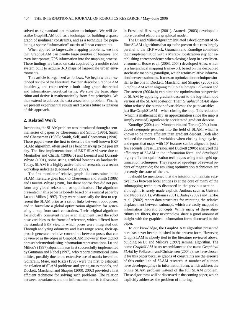
Figure 1 illustrates the GraphSLAM algorithm. Shown thereis the graph that GraphSLAM extracts from four poses labeledx1, . . . , x4, and two map featuresm1, m2. Arcs in this graphcome in two types: motion arcs and measurement arcs. Motionarcs link any two consecutive robot poses, and measurementarcs link poses to features that were measured there. Eachedge in the graph corresponds to a nonlinear constraint. Aswe shall see later, these constraints represent the negative loglikelihood of the measurement and the motion models, henceare best thought of asinformation constraints. Adding such aconstraint to the graph is trivial for GraphSLAM; it involvesno significant computation. The sum of all constraints resultsin a nonlinearleast squares problem, as stated in Figure 1.
To compute a map posterior, GraphSLAM linearizes the setof constraints. The result of linearization is a sparse informa-tion matrix and an information vector. The sparseness of thismatrix enables GraphSLAM to apply the variable eliminationalgorithm, thereby transforming the graph into a much smallerone only defined over robot poses. The path posterior map isthen calculated using standard inference techniques. Graph-SLAM also computes a map and certain marginal posteriorsover the map; the full map posterior is of course quadratic inthe size of the map and hence is usually not recovered.
3.3. Building Up the Graph
Suppose we are given a set of measurementsz1:t with associ-ated correspondence variablesc1:t , and a set of controlsu1:t .GraphSLAM turns this data into a graph. The nodes of thisgraph are the robot posesx1:t and the features in the mapm = {mj }. Each edge in the graph corresponds to an event:a motion event generates an edge between two robot poses,and a measurement event creates a link between a pose and afeature in the map. Edges represent soft constraints betweenposes and features in GraphSLAM.
For a linear system, these constraints are equivalent to en-tries in an information matrix and an information vector of
a large system of equations. As usual, we will denote the in-formation matrix by� and the information vector byξ . Aswe shall see below, each measurement and each control leadsto a local update of� andξ , which corresponds to a localaddition of an edge to the graph in GraphSLAM. In fact, therule for incorporating a control or a measurement into� andξ is a local addition, paying tribute to the important fact thatinformation is an additive quantity.
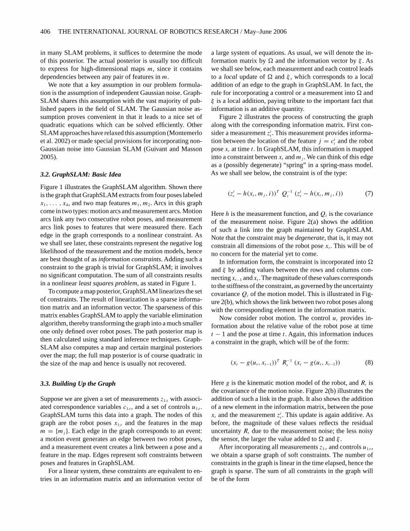
Figure 2 illustrates the process of constructing the graphalong with the corresponding information matrix. First con-sider a measurementzi
t. This measurement provides informa-
tion between the location of the featurej = citand the robot
posext at timet . In GraphSLAM, this information is mappedinto a constraint betweenxt andmj . We can think of this edgeas a (possibly degenerate) “spring” in a spring-mass model.As we shall see below, the constraint is of the type:
(zi
t− h(xt , mj , i))
T Q−1t
(zi
t− h(xt , mj , i)) (7)
Hereh is the measurement function, andQt is the covarianceof the measurement noise. Figure 2(a) shows the additionof such a link into the graph maintained by GraphSLAM.Note that the constraint may bedegenerate, that is, it may notconstrain all dimensions of the robot posext . This will be ofno concern for the material yet to come.
In information form, the constraint is incorporated into�
andξ by adding values between the rows and columns con-nectingxt−1 andxt .The magnitude of these values correspondsto the stiffness of the constraint, as governed by the uncertaintycovarianceQt of the motion model. This is illustrated in Fig-ure 2(b), which shows the link between two robot poses alongwith the corresponding element in the information matrix.
Now consider robot motion. The controlut provides in-formation about the relative value of the robot pose at timet − 1 and the pose at timet . Again, this information inducesa constraint in the graph, which will be of the form:
(xt − g(ut , xt−1))T R−1
t(xt − g(ut , xt−1)) (8)
Hereg is the kinematic motion model of the robot, andRt isthe covariance of the motion noise. Figure 2(b) illustrates theaddition of such a link in the graph. It also shows the additionof a new element in the information matrix, between the posext and the measurementzi
t. This update is again additive. As
before, the magnitude of these values reflects the residualuncertaintyRt due to the measurement noise; the less noisythe sensor, the larger the value added to� andξ .
After incorporating all measurementsz1:t and controlsu1:t ,we obtain a sparse graph of soft constraints. The number ofconstraints in the graph is linear in the time elapsed, hence thegraph is sparse. The sum of all constraints in the graph willbe of the form
Thrun and Montemerlo / The GraphSLAM Algorithm 407
Fig. 1. GraphSLAM illustration, with 4 poses and two map features. Nodes in the graphs are robot poses and featurelocations. The graph is populated by two types of edges: Solid edges which link consecutive robot poses, and dashededges, which link poses with features sensed while the robot assumes that pose. Each link in GraphSLAM is a non-linearquadratic constraint. Motion constraints integrate the motion model; measurement constraints the measurement model. The tar-get function of GraphSLAM is sum of these constraints. Minimizing it yields the most likely map and the most likely robot path.
JGraphSLAM= xT
0 �0 x0 +∑
t
(xt − g(ut , xt−1))T
R−1t
(xt − g(ut , xt−1))
+∑
t
∑i
(zi
t− h(yt , c
i
t, i))T
Q−1t
(zi
t− h(yt , c
i
t, i)) (9)
It is a function defined over pose variablesx1:t and all fea-ture locations in the mapm. Notice that this expression alsofeatures ananchoring constraint of the formxT
0 �0 x0. Thisconstraint anchors the absolute coordinates of the map by ini-tializing the very first pose of the robot as(0 0 0)T .
In the associated information matrix�, the off-diagonalelements are all zero with two exceptions: between any twoconsecutive posesxt−1 andxt will be a non-zero value thatrepresents the information link introduced by the controlut .Also non-zero will be any element between a map featuremj
and a posext , if mj was observed when the robot was atxt .Allelements between pairs of different features remain zero. Thisreflects the fact that we never receive information pertainingto their relative location—all we receive in SLAM are mea-surements that constrain the location of a feature relative toa robot pose. Thus, the information matrix is equally sparse;all but a linear number of its elements are zero.
3.4. Inference
Of course, neither the graph representation nor the informa-tion matrix representation gives us what we want: the map andthe path. In GraphSLAM, the map and the path are obtained
from the linearized information matrix� and the informationvector ξ , via the equations� = �−1 andµ = � ξ . Thisoperation requires us to solve a system of linear equations.This raises the question on how efficiently we can recover themap estimateµ.
The answer to the complexity question depends on thetopology of the world. If each feature is seen only locallyin time, the graph represented by the constraints is linear.Thus,� can be reordered so that it becomes a band-diagonalmatrix, that is, all non-zero values occur near its diagonal. Theequationµ = �−1ξ can then be computed in linear time. Thisintuition carries over to a cycle-free world that is traversedonce, so that each feature is seen for a short, consecutive periodof time.
The more common case, however, involves features thatare observed multiple times, with large time delays in be-tween. This might be the case because the robot goes backand forth through a corridor, or because the world possessescycles. In either situation, there will exist featuresmj thatare seen at drastically different time stepsxt1 andxt2, witht2 � t1. In our constraint graph, this introduces a cyclic depen-dence:xt1 andxt2 are linked through the sequence of controlsut1+1, ut1+2, . . . , ut2 and through the joint observation links be-tweenxt1 andmj , andxt2 andmj , respectively. Such links makeour variable reordering trick inapplicable, and recovering themap becomes more complex. In fact, since the inverse of� ismultiplied with a vector, the result can be computed with op-timization techniques such as conjugate gradient, without ex-plicitly computing the full inverse matrix. Since most worldspossess cycles, this is the case of interest.
408 THE INTERNATIONAL JOURNAL OF ROBOTICS RESEARCH / May–June 2006
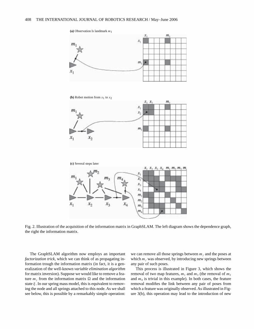
(a) Observation ls landmarkm1
(b) Robot motion fromx1 to x2
(c) Several steps later
Fig. 2. Illustration of the acquisition of the information matrix in GraphSLAM. The left diagram shows the dependence graph,the right the information matrix.
The GraphSLAM algorithm now employs an importantfactorization trick, which we can think of as propagating in-formation trough the information matrix (in fact, it is a gen-eralization of the well-knownvariable elimination algorithmfor matrix inversion). Suppose we would like to remove a fea-turemj from the information matrix� and the informationstateξ . In our spring mass model, this is equivalent to remov-ing the node and all springs attached to this node. As we shallsee below, this is possible by a remarkably simple operation:
we can remove all those springs betweenmj and the poses atwhichmj was observed, by introducing new springs betweenany pair of such poses.
This process is illustrated in Figure 3, which shows theremoval of two map features,m1 andm3 (the removal ofm2
andm4 is trivial in this example). In both cases, the featureremoval modifies the link between any pair of poses fromwhich a feature was originally observed. As illustrated in Fig-ure 3(b), this operation may lead to the introduction of new

Thrun and Montemerlo / The GraphSLAM Algorithm 409
(a) The removal ofm1 changes the link betweenx1 andx2
(b) The removal ofm3 introduces a new link betweenx2 andx4
(c) Final result after removing all map features
Fig. 3. Reducing the graph in GraphSLAM: Arcs are removed to yield a network of links that only connect robot poses.
410 THE INTERNATIONAL JOURNAL OF ROBOTICS RESEARCH / May–June 2006
links in the graph. In the example shown there, the removalof m3 leads to a new link betweenx2 andx4.
Letτ(j) be the set of poses at whichmj was observed (thatis:xt ∈ τ(j)⇐⇒ ∃i : ci
t= j ).Then we already know that the
featuremj is only linked to posesxt in τ(j); by construction,mj is not linked to any other pose, or to any feature in themap. We can now set all links betweenmj and the posesτ(j)
to zero by introducing a new link between any two posesxt , xt ′ ∈ τ(j). Similarly, the information vector values forall posesτ(j) are also updated. An important characteristicof this operation is that it is local: It only involves a smallnumber of constraints. After removing all links tomj , we cansafely removemj from the information matrix and vector.The resulting information matrix is smaller—it lacks an entryfor mj . However, it is equivalent for the remaining variables,in the sense that the posterior defined by this informationmatrix is mathematically equivalent to the original posteriorbefore removingmj . This equivalence is intuitive: We simplyhave replaced springs connectingmj to various poses in ourspring mass model by a set of springs directly linking theseposes. In doing so, the total force asserted by these springsremains equivalent, with the only exception thatmj is nowdisconnected.
The virtue of this reduction step is that we can graduallytransform our inference problem into a smaller one. By re-moving each featuremj from � andξ , we ultimately arriveat a much smaller information form� and ξ defined onlyover the robot path variables. The reduction can be carriedout in time linear in the size of the map; in fact, it generalizesthe variable elimination technique for matrix inversion to theinformation form, in which we also maintain an informationstate. The posterior over the robot path is now recovered as� = �−1 andµ = �ξ . Unfortunately, our reduction step doesnot eliminate cycles in the posterior. The remaining inferenceproblem may still require more than linear time.
As a last step, GraphSLAM recovers the feature locations.Conceptually, this is achieved by building a new informationmatrix �j and information vectorξj for eachmj . Both aredefined over the variablemj and the posesτ(j) at whichmj
were observed. It contains the original links betweenmj andτ(j), but the posesτ(j) are set to the values inµ, withoutuncertainty. From this information form, it is now simple tocalculate the location ofmj , using the common matrix inver-sion trick. Clearly,�j contains only elements that connect tomj ; hence the inversion takes time linear in the number ofposes inτ(j).
It should be apparent why the graph representation is sucha natural representation. The full SLAM problem is solvedby locally adding information into a large information graph,one edge at a time for each measurementzi
tand each control
ut . To turn such information into an estimate of the map andthe robot path, it is first linearized, then information betweenposes and features is gradually shifted to information betweenpairs of poses. The resulting structure only constrains the
robot poses, which are then calculated using matrix inversion.Once the poses are recovered, the feature locations are calcu-lated one after another, based on the original feature-to-poseinformation.
4. The GraphSLAM Algorithm
We will now make the various computational steps of theGraphSLAM precise. The full GraphSLAM algorithm willbe described in a number of steps. The main difficulty inimplementing the simple additive information algorithm per-tains to the conversion of a conditional probability of the formp(zi
t| xt , m) andp(xt | ut , xt−1) into a link in the information
matrix. The information matrix elements are all linear; hencethis step involves linearizingp(zi
t| xt , m) andp(xt | ut , xt−1).
To perform this linearization, we need an initial estimateµ0:tfor all posesx0:t .
There exist a number of solutions to the problem of findingan initial meanµ suitable for linearization. For example, wecan run an EKF SLAM and use its estimate for linearization(Dissanayake et al. 2001). GraphSLAM uses an even sim-pler technique: our initial estimate will simply be providedby chaining together the motion modelp(xt | ut , xt−1). Suchan algorithm is outlined in Table 1, and called thereGraph-SLAM_initialize. This algorithm takes the controlsu1:t as in-put, and outputs sequence of pose estimatesµ0:t . It initializesthe first pose by zero, and then calculates subsequent posesby recursively applying the velocity motion model. Since weare only interested in the mean poses vectorµ0:t , Graph-SLAM_initialize only uses the deterministic part of the mo-tion model. It also does not consider any measurement in itsestimation.
Once an initialµ0:t is available, the GraphSLAM algorithmconstructs the full SLAM information matrix� and the corre-sponding information vectorξ . This is achieved by linearizingthe links in the graph. The algorithmGraphSLAM_linearizeis depicted in Table 2. This algorithm contains a good amountof mathematical notation, much of which will become clearin our derivation of the algorithm further below.Graph-SLAM_linearize accepts as an input the set of controls,u1:t ,the measurementsz1:t and associated correspondence vari-ablesc1:t , and the mean pose estimatesµ0:t . It then graduallyconstructs the information matrix� and the information vec-tor ξ through linearization, by locally adding sub-matrices inaccordance with the information obtained from each measure-ment and each control.
In particular, line 2 inGraphSLAM_linearize initializesthe information elements. The “infinite” information entry inline 3 fixes the initial posex0 to (0 0 0)T . It is necessary, sinceotherwise the resulting matrix becomes singular, reflecting thefact that from relative information alone we cannot recoverabsolute estimates.
Controls are integrated in lines 4 through 9 ofGraph-SLAM_linearize. The posex and the JacobianGt calculated

Thrun and Montemerlo / The GraphSLAM Algorithm 411
Table 1. Initialization of the Mean Pose Vector µ1:tµ1:tµ1:t in the GraphSLAM Algorithm
1: Algorithm GraphSLAM_initialize(u1:t ):
2:
µ0,x
µ0,y
µ0,θ
=
0
00
3: for all controls ut = (vt ωt)T do
4:
µt,x
µt,y
µt,θ
=
µt−1,x
µt−1,y
µt−1,θ
4: + − vt
ωtsinµt−1,θ + vt
ωtsin(µt−1,θ + ωtt)
vt
ωtcosµt−1,θ − vt
ωtcos(µt−1,θ + ωtt)
ωtt
5: endfor6: return µ0:t
Table 2. Calculation of ��� and ξξξ in GraphSLAM
1: Algorithm GraphSLAM_linearize(u1:t , z1:t , c1:t , µ0:t ):
2: set � = 0, ξ = 0
3: add
∞ 0 0
0 ∞ 00 0 ∞
to � at x0
4: for all controls ut = (vt ωt)T do
5: xt = µt−1 + − vt
ωtsinµt−1,θ + vt
ωtsin(µt−1,θ + ωtt)
vt
ωtcosµt−1,θ − vt
ωtcos(µt−1,θ + ωtt)
ωtt
6: Gt = 1 0 vt
ωtcosµt−1,θ − vt
ωtcos(µt−1,θ + ωtt)
0 1 vt
ωtsinµt−1,θ − vt
ωtsin(µt−1,θ + ωtt)
0 0 1
see next page for continuation
412 THE INTERNATIONAL JOURNAL OF ROBOTICS RESEARCH / May–June 2006
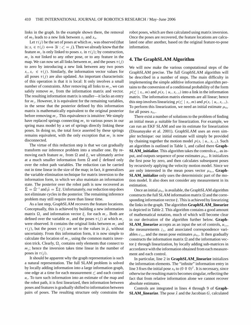
continued from the previous page
7: add
(1−Gt
)R−1
t(1 −Gt) to � at xt and xt−1
8: add
(1−Gt
)R−1
t[xt +Gt µt−1] to ξ at xt and xt−1
9: endfor
10: for all measurements zt do
11: Qt = σr 0 0
0 σφ 00 0 σs
12: for all observed features zit= (ri
tφi
t)T do
13: j = cit
14: δ =(
δx
δy
)=(
µj,x − µt,x
µj,y − µt,y
)15: q = δT δ
16: zit=( √
q
atan2(δy, δx)− µt,θ
)
17: Hit= 1
q
( √qδx −√qδy 0 −√qδx
√qδy
δy δx −1 −δy −δx
)18: add HiT
tQ−1
tH i
tto � at xt and mj
19: add HiTt
Q−1t[ zi
t− zi
t−Hi
t
µt,x
µt,y
µt,θ
µj,x
µj,y
] to ξ at xt and mj
20: endfor
21: endfor
22: return �, ξ
in lines 5 and 6 represent the linear approximation of thenon-linear measurement functiong. As is obvious from theseequations, this linearization step utilizes the pose estimatesµ0:t−1, with µ0 = (0 0 0)T . This leads to the updates for�,andξ , calculated in lines 7, and 8, respectively. Both termsare added into the corresponding rows and columns of� andξ . This addition realizes the inclusion of a new constraint intothe SLAM posterior, very much along the lines of the intuitivedescription in the previous section.
Measurements are integrated in lines 10 through 21 ofGraphSLAM_linearize. The matrixQt calculated in line11 is the familiar measurement noise covariance. Lines 13through 17 compute the Taylor expansion of the measurementfunction. This calculation assumesknown correspondence be-
tween observed features and features in the map (line 13). At-tention has to be paid to the implementation of line 16, sincethe angular expressions can be shifted arbitrarily by 2π . Thiscalculation culminates in the computation of the measurementupdate in lines 18 and 19. The matrix that is being added to� in line 18 is of dimension 5× 5. To add it, we decomposeit into a matrix of dimension 3× 3 for the posext , a matrixof dimension 2× 2 for the featuremj , and two matrices ofdimension 3× 2 and 2× 3 for the link betweenxt andmj .Those are added to� at the corresponding rows and columns.Similarly, the vector added to the information vectorξ is ofvertical dimension 5. It is also chopped into two vectors ofsize 3 and 2, and added to the elements corresponding toxt
andmj , respectively. The result ofGraphSLAM_linearize

Thrun and Montemerlo / The GraphSLAM Algorithm 413
is an information vectorξ and a matrix�. We already notedthat� is sparse. It contains only non-zero sub-matrices alongthe main diagonal, between subsequent poses, and betweenposes and features in the map. The running time of this al-gorithm is linear int , the number of time steps at which datawas accrued.
The next step of the GraphSLAM algorithm pertains toreducing the dimensionality of the information matrix/vector.This is achieved through the algorithmGraphSLAM_reducein Table 3. This algorithm takes as input� and ξ definedover the full space of map features and poses, and outputs areduced matrix� and vectorsξ defined over the space of allposes (but not the map!). This transformation is achieved byremoving featuresmj one at a time, in lines 4 through 9 ofGraphSLAM_reduce. The bookkeeping of the exact indexesof each item in� and ξ is a bit tedious, hence Table 3 onlyprovides an intuitive account.
Line 5 calculates the set of posesτ(j) at which the robotobserved featurej . It then extracts two sub-matrices from thepresent�: �j,j and�τ(j),j . �j,j is the quadratic sub-matrix be-tweenmj andmj , and�τ(j),j is composed of the off-diagonalelements betweenmj and the pose variablesτ(j). It also ex-tracts from the information state vectorξ the elements cor-responding to thej -th feature, denoted here asξj . It thensubtracts information from� andξ as stated in lines 6 and 7.After this operation, the rows and columns for the featuremj
are zero. These rows and columns are then removed, reducingthe dimension on� andξ accordingly. This process is iterateduntil all features have been removed, and only pose variablesremain in� andξ . The complexity ofGraphSLAM_reduceis once again linear int .
The last step in the GraphSLAM algorithm computes themean and covariance for all poses in the robot path, and amean location estimate for all features in the map. This isachieved throughGraphSLAM_solve inTable 4. Line 3 com-putes the path estimatesµ0:t . This can be achieved by invertingthe reduced information matrix� and multiplying the result-ing covariance with the information vector, or by optimizationtechniques such as conjugate gradient descent. Subsequently,GraphSLAM_solve computes the location of each feature inlines 4 through 7. The return value ofGraphSLAM_solvecontains the mean for the robot path and all features in themap, but only the covariance for the robot path.
The quality of the solution calculated by the GraphSLAMalgorithm depends on the goodness of the initial mean es-timates, calculated byGraphSLAM_initialize. Thex- andy-components of these estimates affect the respective modelsin a linear way, hence the linearization does not depend onthese values. Not so for the orientation variables inµ0:t . Er-rors in these initial estimates affect the accuracy of the Taylorapproximation, which in turn affects the result.
To reduce potential errors due to the Taylor approximationin the linearization, the proceduresGraphSLAM_linearize,GraphSLAM_reduce, and GraphSLAM_solve are run
multiple times over the same data set. Each iteration takesas an input an estimated mean vectorµ0:t from the previousiteration, and outputs a new, improved estimate. The iterationsof the GraphSLAM optimization are only necessary when theinitial pose estimates have high error (e.g. more than 20 de-grees orientation error). A small number of iterations (e.g. 3)is usually sufficient.
Table 5 summarizes the resulting algorithm. It initializesthe means, then repeats the construction step, the reductionstep, and the solution step. Typically, two or three iterationssuffice for convergence.The resulting meanµ is our best guessof the robot’s path and the map.
5. Mathematical Derivation of GraphSLAM
The derivation of the GraphSLAM algorithm begins witha derivation of a recursive formula for calculating the fullSLAM posterior, represented in information form. We theninvestigate each term in this posterior, and derive from themthe additive SLAM updates through Taylor expansions. Fromthat, we will derive the necessary equations for recovering thepath and the map.
5.1. The Full SLAM Posterior
It will be beneficial to introduce a variable for the augmentedstate of the full SLAM problem. We will usey to denote statevariables that combine one or more posesx with the mapm.In particular, we definey0:t to be a vector composed of the pathx0:t and the mapm, whereasyt is composed of the momentarypose at timet and the mapm:
y0:t =
x0
x1
...
xt
m
and yt =
(xt
m
)(10)
The posterior in the full SLAM problem isp(y0:t |z1:t , u1:t , c1:t ), wherez1:t are the familiar measurements withcorrespondencesc1:t , andu1:t are the controls. Bayes rule en-ables us to factor this posterior:
p(y0:t | z1:t , u1:t , c1:t ) (11)
= η p(zt | y0:t , z1:t−1, u1:t , c1:t ) p(y0:t | z1:t−1, u1:t , c1:t )
whereη is the familiar normalizer. The first probability on theright-hand side can be reduced by dropping irrelevant condi-tioning variables:
p(zt | y0:t , z1:t−1, u1:t , c1:t ) = p(zt | yt , ct ) (12)

414 THE INTERNATIONAL JOURNAL OF ROBOTICS RESEARCH / May–June 2006
Table 3. Algorithm for Reducing the Size of the Information Representation of the Posteriorin GraphSLAM
1: Algorithm GraphSLAM_reduce(�, ξ ):
2: � = �
3: ξ = ξ
4: for each feature j do
5: let τ(j) be the set of all poses xt at which j was observed
6: subtract �τ(j),j �−1j,j ξj from ξ at xτ(j) and mj
7: subtract �τ(j),j �−1j,j �j,τ (j) from � at xτ(j) and mj
8: remove from � and ξ all rows/columns corresponding to j
9: endfor
10: return �, ξ
Table 4. Algorithm for Updating the Posterior µµµ
1: Algorithm GraphSLAM_solve(�, ξ , �, ξ ):
2: �0:t = �−1
3: µ0:t = �0:t ξ
4: for each feature j do
5: set τ(j) to the set of all poses xt at which j was observed
6: µj = �−1j,j (ξj +�j,τ(j) µτ(j))
7: endfor
8: return µ, �0:t
Table 5. The GraphSLAM Algorithm for the Full SLAM Problem with KnownCorrespondence
1: Algorithm GraphSLAM_known_correspondence(u1:t , z1:t , c1:t ):
2: µ0:t = GraphSLAM_initialize(u1:t )
3: repeat
4: �, ξ = GraphSLAM_linearize(u1:t , z1:t , c1:t , µ0:t )
5: �, ξ = GraphSLAM_reduce(�, ξ)
6: µ, �0:t = GraphSLAM_solve(�, ξ , �, ξ)
7: until convergence
8: return µ

Thrun and Montemerlo / The GraphSLAM Algorithm 415
Similarly, we can factor the second probability by partitioningy0:t into xt andy0:t−1, and obtain:
p(y0:t | z1:t−1, u1:t , c1:t ) (13)
= p(xt | y0:t−1, z1:t−1, u1:t , c1:t ) p(y0:t−1 | z1:t−1, u1:t , c1:t )
= p(xt | xt−1, ut ) p(y0:t−1 | z1:t−1, u1:t−1, c1:t−1)
Putting these expressions back into (11) gives us the recursivedefinition of the full SLAM posterior:
p(y0:t | z1:t , u1:t , c1:t ) (14)
= η p(zt | yt , ct )
p(xt | xt−1, ut ) p(y0:t−1 | z1:t−1, u1:t−1, c1:t−1)
The closed form expression is obtained through induction overt . Herep(y0) is the prior over the mapm and the initial posex0.
p(y0:t | z1:t , u1:t , c1:t ) (15)
= η p(y0)∏
t
p(xt | xt−1, ut ) p(zt | yt , ct )
= η p(y0)∏
t
[p(xt | xt−1, ut )
∏i
p(zi
t| yt , c
i
t)
]
Here, as before,zitis thei-th measurement in the measurement
vectorzt at timet . The priorp(y0) factors into two indepen-dent priors,p(x0) andp(m). In SLAM, we usually have noprior knowledge about the mapm. We simply replacep(y0)
by p(x0) and subsume the factorp(m) into the normalizerη.
5.2. The Negative Log Posterior
The information form represents probabilities in logarithmicform. The log-SLAM posterior follows directly from the pre-vious equation:
logp(y0:t | z1:t , u1:t , c1:t ) (16)
= const.+ logp(x0)
+∑
t
[logp(xt | xt−1, ut ) +
∑i
logp(zi
t| yt , c
i
t)
]
As stated above, we assume the outcome of robot motion isdistributed normally according toN (g(ut , xt−1), Rt), wheregis the deterministic motion function, andRt is the covarianceof the motion error. Likewise, measurementszi
tare gener-
ated according toN (h(yt , cit, i), Qt), whereh is the familiar
measurement function andQt is the measurement error co-
variance. In equations, we have:
p(xt | xt−1, ut ) (17)
= η exp
{−1
2(xt − g(ut , xt−1))
T R−1t
(xt − g(ut , xt−1))
}p(zi
t| yt , c
i
t) (18)
= η exp
{−1
2(zi
t− h(yt , c
i
t, i))T Q−1
t(zi
t− h(yt , c
i
t, i))
}The priorp(x0) in (16) is also easily expressed by a Gaussian-type distribution. Itanchors the initial posex0 to the origin ofthe global coordinate system:x0 = (0 0 0)T :
p(x0) = η exp
{−1
2xT
0 �0 x0
}(19)
with
�0 = ∞ 0 0
0 ∞ 00 0 ∞
(20)
For now, it does not concern us that the value of∞ cannotbe implemented, as we can easily substitute∞ with a largepositive number. This leads to the following quadratic formof the negative log-SLAM posterior in (16):
− logp(y0:t | z1:t , u1:t , c1:t ) (21)
= const.+ 1
2
[xT
0 �0 x0 +∑
t
(xt − g(ut , xt−1))T
R−1t
(xt − g(ut , xt−1))+∑
t
∑i
(zi
t− h(yt , c
i
t, i))T
Q−1t
(zi
t− h(yt , c
i
t, i))
]This is essentially the same asJGraphSLAM in eq. (9), with afew differences pertaining to the omission of normalizationconstants (including a multiplication with−1). Equation (21)highlights an essential characteristic of the full SLAM poste-rior in the information form: it is composed of a number ofquadratic terms, one for the prior, and one for each controland each measurement.
5.3. Taylor Expansion
The various terms in eq. (21) are quadratic in the functionsg
andh, not in the variables we seek to estimate (poses and themap). GraphSLAM alleviates this problem bylinearizing g
andh via Taylor expansion. In particular, we have:
g(ut , xt−1) ≈ g(ut , µt−1)+ g′(ut , µt−1)︸ ︷︷ ︸=: Gt
(xt−1 − µt−1) (22)
h(yt , ci
t, i) ≈ h(µt, c
i
t, i) + h′(µt)︸ ︷︷ ︸
=: Hit
(yt − µt) (23)
416 THE INTERNATIONAL JOURNAL OF ROBOTICS RESEARCH / May–June 2006
Here µt is the current estimate of the state vectoryt , andHi
t= hi
tFx,j for the projection matrixFx,j as indicated.
This linear approximation turns the log-likelihood (21) intoa function that is quadratic iny0:t . In particular, we obtain:
logp(y0:t | z1:t , u1:t , c1:t ) = const.− 1
2(24){
xT
0 �0 x0 +∑
t
[xt − g(ut , µt−1)−Gt(xt−1 − µt−1)]T
R−1t[xt − g(ut , µt−1)−Gt(xt−1 − µt−1)]
+∑
i
[zi
t− h(µt, c
i
t, i)−Hi
t(yt − µt)]T
Q−1t[zi
t− h(µt, c
i
t, i)−Hi
t(yt − µt)]
}This function is indeed a quadratic iny0:t , and it is convenientto reorder its terms, omitting several constant terms.
logp(y0:t | z1:t , u1:t , c1:t ) = const. (25)
− 1
2xT
0 �0 x0︸ ︷︷ ︸quadratic inx0
− 1
2
∑t
xT
t−1:t
(1−Gt
)R−1
t(1 −Gt) xt−1:t︸ ︷︷ ︸
quadratic inxt−1:t
+ xT
t−1:t
(1−Gt
)R−1
t[g(ut , µt−1)+Gt µt−1]︸ ︷︷ ︸
linear in xt−1:t
− 1
2
∑i
yT
tH iT
tQ−1
tH i
tyt︸ ︷︷ ︸
quadratic inyt
+ yT
tH iT
tQ−1
t[zi
t− h(µt, c
i
t, i)−Hi
tµt ]︸ ︷︷ ︸
linear in yt
Herext−1:t denotes the vector concatenatingxt−1 andxt ; hencewe can write(xt−Gt xt−1)
T = xTt−1:t (1 −Gt)
T . If we collectall quadratic terms into the matrix�, and all linear terms intoa vectorξ , we see that expression (24) is of the form:
logp(y0:t | z1:t , u1:t , c1:t ) = const.− 1
2yT
0:t � y0:t + yT
0:t ξ (26)
5.4. Constructing the Information Form
We can read off these terms directly from (25), and verifythat they are indeed implemented in the algorithmGraph-SLAM_linearize in Table 2:
• Prior. The initial pose prior manifests itself by aquadratic term�0 over the initial pose variablex0 inthe information matrix. Assuming appropriate exten-sion of the matrix�0 to match the dimension ofy0:t , wehave:
� ←− �0 (27)
This initialization is performed in lines 2 and 3 of thealgorithmGraphSLAM_linearize.
• Controls. From (25), we see that each controlut adds to� andξ the following terms, assuming that the matricesare rearranged so as to be of matching dimensions:
�←− �+(
1−Gt
)R−1
t(1 −Gt) (28)
ξ ←− ξ +(
1−Gt
)R−1
t[g(ut , µt−1)+Gt µt−1]
(29)
This is realized in lines 4 through 9 inGraph-SLAM_linearize.
• Measurements. According to eq. (25), each measure-mentzi
ttransforms� andξ by adding the following
terms, once again assuming appropriate adjustment ofthe matrix dimensions:
�←− �+HiT
tQ−1
tH i
t(30)
ξ ←− ξ +HiT
tQ−1
t[zi
t− h(µt, c
i
t, i)−Hi
tµt ] (31)
This update occurs in lines 10 through 21 inGraph-SLAM_linearize.
This proves the correctness of the construction algorithmGraphSLAM_linearize, relative to our Taylor expansionapproximation.
We also note that the steps above only affect off-diagonalelements that involve at least one pose. Thus, all between-feature elements are zero in the resulting information matrix.
5.5. Reducing the Information Form
The reduction stepGraphSLAM_reduce is based on a fac-torization of the full SLAM posterior.
p(y0:t | z1:t , u1:t , c1:t ) = p(x0:t | z1:t , u1:t , c1:t ) (32)
p(m | x0:t , z1:t , u1:t , c1:t )
Herep(x0:t | z1:t , u1:t , c1:t ) ∼ N (�, ξ) is the posterior overpaths alone, with the map integrated out:
p(x0:t | z1:t , u1:t , c1:t ) =∫
p(y0:t | z1:t , u1:t , c1:t ) dm (33)
As we will show shortly, this probability is indeed calculatedby the algorithmGraphSLAM_reduce in Table 3, since
p(x0:t | z1:t , u1:t , c1:t ) ∼ N (ξ , �) (34)
In general, the integration in (33) will be intractable, due to thelarge number of variables inm. For Gaussians, this integralcan be calculated in closed form. The key insight is given bythemarginalization lemma for Gaussians, stated in Table 7.

Thrun and Montemerlo / The GraphSLAM Algorithm 417
Table 6. The (Specialized) Inversion Lemma, Sometimes Called the Sherman/MorrisonFormula (see the Appendix for a derivation)
Inversion Lemma. For any invertible quadratic matricesR andQand any matrixP with appropriatedimensions, the following holds true
(R + P Q P T )−1 = R−1 − R−1 P (Q−1 + P T R−1 P)−1 P T R−1
assuming that all above matrices can be inverted as stated.
Table 7. Lemma for Marginalizing Gaussians in Information Form. The Form of theCovariance �xx�xx�xx in This Lemma is Also as Schur complement (a derivation can be foundin the Appendix).Marginals of a multivariate Gaussian. Let the probability distributionp(x, y) over the randomvectorsx andy be a Gaussian represented in the information form
� =(
�xx �xy
�yx �yy
)and ξ =
(ξx
ξy
)
If �yy is invertible, the marginalp(x) is a Gaussian whose information representation is
�xx = �xx −�xy �−1yy
�yx and ξx = ξx −�xy �−1yy
ξy
Let us subdivide the matrix� and the vectorξ into sub-matrices, for the robot pathx0:t and the mapm:
� =(
�x0:t ,x0:t �x0:t ,m�m,x0:t �m,m
)(35)
ξ =(
ξx0:tξm
)(36)
According to themarginalization lemma, the probability (34)is obtained as
� = �x0:t ,x0:t −�x0:t ,m �−1m,m
Ømegam,x0:t (37)
ξ = ξx0:t −�x0:t ,m �−1m,m
ξm (38)
The matrix�m,m is block-diagonal. This follows from the way� is constructed, in particular the absence of any links be-tween pairs of features. This makes the inversion efficient:
�−1m,m=
∑j
F T
j�−1
j,jFj (39)
where�j,j = Fj�F Tj
is the sub-matrix of� that correspondsto thej -th feature in the map, that is
Fj = 0 · · ·0 1 0 0· · ·0
0 · · ·0 0 1︸︷︷︸j−th feature
0 · · ·0 (40)
This insight makes it possible to decompose the implement
eqs (37) and (38) into a sequential update:
� = �x0:t ,x0:t −∑
j
�x0:t ,j �−1j,j;�j,x0:t (41)
ξ = ξx0:t −∑
j
�x0:t ,j �−1j,j
ξj (42)
The matrix�x0:t ,j is non-zero only for elements inτ(j), theset of poses at which featurej was observed. This essentiallyproves the correctness of the reduction algorithmGraph-SLAM_reduce in Table 3. The operation performed on�in this algorithm can be thought of as the variable eliminationalgorithm for matrix inversion, applied to the feature variablesbut not the robot pose variables.
5.6. Recovering the Path and the Map
The algorithmGraphSLAM_solve in Table 4 calculates themean and variance of the GaussianN (ξ , �):
� = �−1 (43)
µ = � ξ (44)
In particular, this operation provides us with the mean of theposterior on the robot path; it does not give us the locationsof the features in the map.
It remains to recover the second factor of eq. (32):
p(m | x0:t , z1:t , u1:t , c1:t ) (45)

418 THE INTERNATIONAL JOURNAL OF ROBOTICS RESEARCH / May–June 2006
Table 8. Lemma for Conditioning Gaussians in Information Form (a derivation can be foundin the Appendix)Conditionals of a multivariate Gaussian. Let the probability distributionp(x, y) over the randomvectorsx andy be a Gaussian represented in the information form
� =(
�xx �xy
�yx �yy
)and ξ =
(ξx
ξy
)
The conditionalp(x | y) is a Gaussian with information matrix�xx and information vectorξx +�xy y.
The conditioning lemma, stated in Table 8, shows that thisprobability distribution is Gaussian with the parameters
�m = �−1m,m
(46)
µm = �m(ξm +�m,x0:t ξ ) (47)
Hereξm and�m,m are the sub-vector ofξ , and the sub-matrixof �, respectively, restricted to the map variables. The matrix�m,x0:t is the off-diagonal sub-matrix of� that connects therobot path to the map.As noted before,�m,m is block-diagonal,hence we can decompose
p(m | x0:t , z1:t , u1:t , c1:t ) =∏
j
p(mj | x0:t , z1:t , u1:t , c1:t ) (48)
where eachp(mj | x0:t , z1:t , u1:t , c1:t ) is distributed accord-ing to
�j = �−1j,j
(49)
µj = �j(ξj +�j,x0:t µ) = �j(ξj +�j,τ(j)µτ(j)) (50)
The last transformation exploited the fact that the sub-matrix�j,x0:t is zero except for those pose variablesτ(j) from whichthej -th feature was observed.
It is important to notice that this is a Gaussianp(m |x0:t , z1:t , u1:t , c1:t ) conditioned on the true pathx0:t . In prac-tice, we do not know the path, hence one might want to knowthe posteriorp(m | z1:t , u1:t , c1:t ) without the path in the condi-tioning set. This Gaussian cannot be factored in the momentsparameterization, as locations of different features are cor-related through the uncertainty over the robot pose. For thisreason,GraphSLAM_solve returns the mean estimate of theposterior but only the covariance over the robot path. Luckily,we never need the full Gaussian in moments representation—which would involve a fully populated covariance matrix ofmassive dimensions—as all essential questions pertaining tothe SLAM problem can be answered at least in approximationwithout knowledge of�.
6. Data Association in GraphSLAM
Data association in GraphSLAM is realized through corre-spondence variables. GraphSLAM searches for a single best
correspondence vector, instead of calculating an entire distri-bution over correspondences. Thus, finding a correspondencevector is a search problem. However, it proves convenient todefine correspondences slightly differently in GraphSLAMthan before: correspondences are defined over pairs of fea-tures in the map, rather than associations of measurements tofeatures. Specifically, we sayc(j, k) = 1 if mj andmk corre-spond to the same physical feature in the world. Otherwise,c(j, k) = 0. This feature-correspondence is in fact logicallyequivalent to the correspondence defined in the previous sec-tion, but it simplifies the statement of the basic algorithm.
Our technique for searching the space of correspondencesis greedy, just as in the EKF. Each step in the search of the bestcorrespondence value leads to an improvement, as measuredby the appropriate log-likelihood function. However, becauseGraphSLAM has access to all data at the same time, it is possi-ble to devise correspondence techniques that are considerablymore powerful than the incremental approach in the EKF. Inparticular:
1. At any point in the search, GraphSLAM can con-sider the correspondence of any set of features. Thereis no requirement to process the observed featuressequentially.
2. Correspondence search can be combined with the cal-culation of the map. Assuming that two observed fea-tures correspond to the same physical feature in theworld affects the resulting map. By incorporating sucha correspondence hypothesis into the map, other corre-spondence hypotheses will subsequently look more orless likely.
3. Data association decisions in GraphSLAM can be un-done. The goodness of a data association depends onthe value of other data association decisions. What ap-pears to be a good choice early on in the search may, atsome later time in the search, turn out to be inferior. Toaccommodate such a situation, GraphSLAM can effec-tively undo a previous data association decision.
We will now describe one specific correspondence search al-gorithm that exploits the first two properties, but not the third.

Thrun and Montemerlo / The GraphSLAM Algorithm 419
Our data association algorithm will still be greedy, and it willsequentially search the space of possible correspondences toarrive at a plausible map. However, like all greedy algorithms,our approach is subject to local maxima; the true space ofcorrespondences is of course exponential in the number offeatures in the map. Nevertheless, we will be content with ahill climbing algorithm.
6.1. The GraphSLAM Algorithm with UnknownCorrespondence
The key component of our algorithm is alikelihood test forcorrespondence. Specifically, GraphSLAM correspondenceis based on a simple test: what is the probability that twodifferent features in the map,mj andmk, correspond to thesame physical feature in the world? If this probability exceedsa threshold, we will accept this hypothesis and merge bothfeatures in the map.
The algorithm for the correspondence test is depicted inTable 9: the input to the test are two feature indexes,j andk, for which we seek to compute the probability that thosetwo features correspond to the same feature in the physicalworld. To calculate this probability, our algorithm utilizes anumber of quantities: the information representation of theSLAM posterior, as manifest by� andξ , and the result of theprocedureGraphSLAM_solve, which is the mean vectorµand the path covariance�0:t .
The correspondence test then proceeds in the followingway. First, it computes the marginalized posterior over thetwo target features. This posterior is represented by the in-formation matrix�[j,k] and vectorξ[j,k] computed in lines 2and 3 in Table 9. This step of the computation utilizes varioussub-elements of the information form�, ξ , the mean featurelocations as specified throughµ, and the path covariance�0:t .Next, it calculates the parameters of a new Gaussian randomvariable, whose value is the difference betweenmj andmk.Denoting the difference variablej,k = mj−mk, the informa-tion parameters�j,k, ξj,k are calculated in lines 4 and 5, andthe corresponding expectation for the difference is computedin line 6. Line 7 returns the probability that the differencebetweenmj andmk is zero.
The correspondence test provides us with an algorithmfor performing data association search in GraphSLAM. Ta-ble 10 shows such an algorithm. It initializes the correspon-dence variables with unique values. The four steps that follow(lines 3-7) are the same as in our GraphSLAM algorithm withknown correspondence, stated in Table 5. However, this gen-eral SLAM algorithm then engages in the data associationsearch. Specifically, for each pair of different features in themap, it calculates the probability of correspondence (line 9in Table 10). If this probability exceeds a thresholdχ , thecorrespondence vectors are set to the same value (line 11).
The GraphSLAM algorithm iterates the construction, re-duction, and solution of the SLAM posterior (lines 12 through
14).As a result, subsequent correspondence tests factor in pre-vious correspondence decisions though a newly constructedmap. The map construction is terminated when no further fea-tures are found in its inner loop.
Clearly, the algorithmGraphSLAM is not particularly ef-ficient. In particular, it tests all feature pairs for correspon-dence, not just nearby ones. Further, it reconstructs the mapwhenever a single correspondence is found; rather than pro-cessing sets of corresponding features in batch. Such modifi-cations, however, are relatively straightforward. A good im-plementation ofGraphSLAM will be more refined than ourbasic implementation discussed here.
6.2. Mathematical Derivation of the Correspondence Test
We essentially restrict our derivation to showing the correct-ness of the correspondence test in Table 9. Our first goal isto define a posterior probability distribution over a variablej,k = mj − mk, thedifference between the location of fea-turemj and featuremk. Two featuresmj andmk are equivalentif and only if their location is the same. Hence, by calculat-ing the posterior probability ofj,k, we obtain the desiredcorrespondence probability.
We obtain the posterior forj,k by first calculating the jointovermj andmk:
p(mj, mk | z1:t , u1:t , c1:t ) (51)
=∫
p(mj, mk | x1:t , z1:t , c1:t ) p(x1:t | z1:t , u1:t , c1:t ) dx1:t
We will denote the information form of this marginal posteriorby ξ[j,k] and�[j,k]. Note the use of the squared brackets, whichdistinguish these values from the sub-matrices of the jointinformation form.
The distribution (51) is obtained from the joint posteriorovery0:t , by applying the marginalization lemma. Specifically,� andξ represent the joint posterior over the full state vectory0:t in information form, andτ(j) andτ(k) denote the setsof poses at which the robot observed featurej , and featurek,respectively. GraphSLAM gives us the mean pose vectorµ.Toapply the marginalization lemma (Table 7), we shall leveragethe result of the algorithmGraphSLAM_solve. Specifically,GraphSLAM_solve provides us with a mean for the featuresmj andmk. We simply restate the computation here for thejoint feature pair:
µ[j,k] = �−1jk,jk
(ξjk +�jk,τ(j,k)µτ(j,k)) (52)
Hereτ(j, k) = τ(j)∪ τ(k) denotes the set of poses at whichthe robot observedmj or mk.
For the joint posterior, we also need a covariance. Thiscovariance isnot computed inGraphSLAM_solve, simplybecause the joint covariance over multiple features requiresspace quadratic in the number of features. However, for pairsof features the covariance of the joint is easily recovered.

420 THE INTERNATIONAL JOURNAL OF ROBOTICS RESEARCH / May–June 2006
Table 9. The GraphSLAM Test for Correspondence: It Accepts as Input an InformationRepresentation of the SLAM Posterior, Along with the Result of the GraphSLAM_solve Step.It Then Outputs the Posterior Probability That mjmjmj Corresponds to mkmkmk.
1: Algorithm GraphSLAM_correspondence_test(�, ξ, µ, �0:t , j, k):
2: �[j,k] = �jk,jk −�jk,τ(j,k) �τ(j,k),τ (j,k) �τ(j,k),jk
3: ξ[j,k] = �[j,k] µj,k
4: �j,k =(
1
−1
)T
�[j,k]
(1
−1
)
5: ξj,k =(
1
−1
)T
ξ[j,k]
6: µj,k = �−1j,k ξj,k
7: return |2π �−1j,k|− 1
2 exp{− 1
2µT
j,k�−1
j,k µj,k
}
Table 10. The GraphSLAM Algorithm for the Full SLAM Problem with UnknownCorrespondence. The inner loop of this algorithm can be made more efficient by selectiveprobing feature pairs mj, mkmj , mkmj , mk, and by collecting multiple correspondences before solvingthe resulting collapsed set of equations.
1: Algorithm GraphSLAM(u1:t , z1:t ):
2: initialize all cit
with a unique value
3: µ0:t = GraphSLAM_initialize(u1:t )
4: �, ξ = GraphSLAM_linearize(u1:t , z1:t , c1:t , µ0:t )
5: �, ξ = GraphSLAM_reduce(�, ξ)
6: µ, �0:t = GraphSLAM_solve(�, ξ , �, ξ)
7: repeat
8: for each pair of non-corresponding features mj, mk do
9: πj=k = GraphSLAM_correspondence_test(�, ξ, µ, �0:t , j, k)
10: if πj=k > χ then
11: for all cit= k set ci
t= j
12: �, ξ = GraphSLAM_linearize(u1:t , z1:t , c1:t , µ0:t )
13: �, ξ = GraphSLAM_reduce(�, ξ)
14: µ, �0:t = GraphSLAM_solve(�, ξ , �, ξ)
15: endif
16: endfor
17: until no more pair mj, mk found with πj=k < χ
18: return µ

Thrun and Montemerlo / The GraphSLAM Algorithm 421
Let �τ(j,k),τ (j,k) be the sub-matrix of the covariance�0:t re-stricted to all poses inτ(j, k). Here the covariance�0:t is cal-culated in line 2 of the algorithmGraphSLAM_solve. Thenthe marginalization lemma provides us with the marginal in-formation matrix for the posterior over(mj mk)
T :
�[j,k] = �jk,jk −�jk,τ(j,k) �τ(j,k),τ (j,k) �τ(j,k),jk (53)
The information form representation for the desired posterioris now completed by the following information vector:
ξ[j,k] = �[j,k] µ[j,k] (54)
Hence for the joint we have:
p(mj, mk | z1:t , u1:t , c1:t ) (55)
= η exp
{−1
2
(mj
mk
)T
�[j,k]
(mj
mk
)
+(
mj
mk
)T
ξ[j,k]
}
These equations are identical to lines 2 and 3 in Table 9.The useful thing about our representation is that it imme-
diately lets us define the desired correspondence probability.For that, let us consider the random variable:
j,k = mj − mk (56)
=(
1−1
)T (mj
mk
)
=(
mj
mk
)T (1−1
)
Plugging this into the definition of a Gaussian in informationrepresentation, we obtain:
p(j,k | z1:t , u1:t , c1:t ) (57)
= η exp
−
1
2T
j,k
(1−1
)T
�[j,k]
(1−1
)︸ ︷︷ ︸
=: �j,k
j,k
+ T
j,k
(1−1
)T
ξ[j,k]︸ ︷︷ ︸=: ξj,k
= η exp
{−1
2T
j,k�j,k +T
j,kξj,k
}T
which is Gaussian with the information matrix�j,k and in-formation vectorξj,k as defined above. To calculate the prob-ability that this Gaussian assumes the value ofj,k = 0, it is
useful to rewrite this Gaussian in moments parameterization:
p(j,k | z1:t , u1:t , c1:t ) (58)
= |2π �−1j,k|− 1
2
exp
{−1
2(j,k − µj,k)
T �−1j,k
(j,k − µj,k)
}
where the mean is given by the obvious expression:
µj,k = �−1j,k
ξj,k (59)
These steps are found in lines 4 through 6 in Table 9.The desired probability forj,k = 0 is the result of plug-
ging 0 into this distribution, and reading off the resulting prob-ability:
p(j,k = 0 | z1:t , u1:t , c1:t ) = |2π �−1j,k|− 1
2 (60)
exp
{−1
2µT
j,k�−1
j,kµj,k
}
This expression is the probability that two features in the map,mj andmk, correspond to the same features in the map. Thiscalculation is implemented in line 7 in Table 9.
7. Results
We conducted a number of experiments, all with the robotshown in Figure 4. In particular, we mapped a number of urbansites, including NASA’s Search and Rescue Facility DARTand a large fraction of Stanford’s main campus; snapshots ofthese experiments will be discussed below.
Our experiments either involved the collection of a sin-gle large dataset, or a number of datasets. The latter becamenecessary since for the environments of the size studied here,the robot possesses insufficient battery capacity to collect alldata within a single run. In most experiments, the robot iscontrolled manually. This is necessary because the urban en-vironments are usually populated with moving objects, suchas cars, which would otherwise run the danger of collidingwith our robot. We have, on several occasions, used our navi-gation package Carmen (Montemerlo, Roy, and Thrun 2003)to drive the robot autonomously, validating the terrain analysistechniques discussed above.
Our research has led to a number of results. A primaryfinding is that with our representation, maps with more than108 variables can be computed quickly, even under multipleloop-closure constraints. The time for thinning the networkinto its skeleton tends to take linear time in the number ofrobot poses, which is the same order as the time required fordata collection. We find that scan matching is easily achievedin real-time, as the robot moves, using a portable laptop com-puter. This is a long-known result for horizontally mounted

422 THE INTERNATIONAL JOURNAL OF ROBOTICS RESEARCH / May–June 2006
Fig. 4. The Segbot, a robot based on the Segway RMP platform and developed through the DARPA MARS program.
Fig. 5. Data acquisition through a two-directional scanning laser (the blue stripe indicates a vertical scan). The coloringindicates the result of terrain analysis: The ground surface is colored in green, obstacles are red, and structure above therobot’s reach are shown in white.
laser range finders, but it is reassuring that the same appliesto the more difficult scan matching problem involving a verti-cally panning scanner. More importantly, the relaxation of thepose potentials takes in the order of 30 seconds even for thelargest data set used in our research, of an area 600 m by 800 min size, and with a dozen cycles. This suggests the appropriate-ness of our representation an algorithms for large-scale urbanmapping.
The second result pertains to the utility of GPS data forindoor maps. GPS measurements are easily incorporated intoGraphSLAM; they form yet another arc in the graph of con-straints.We find that indoor maps become more accurate whensome of the data is collected outdoors, where GPS measure-ments are available. Below, we will discuss an experimentalsnapshot that documents this result.
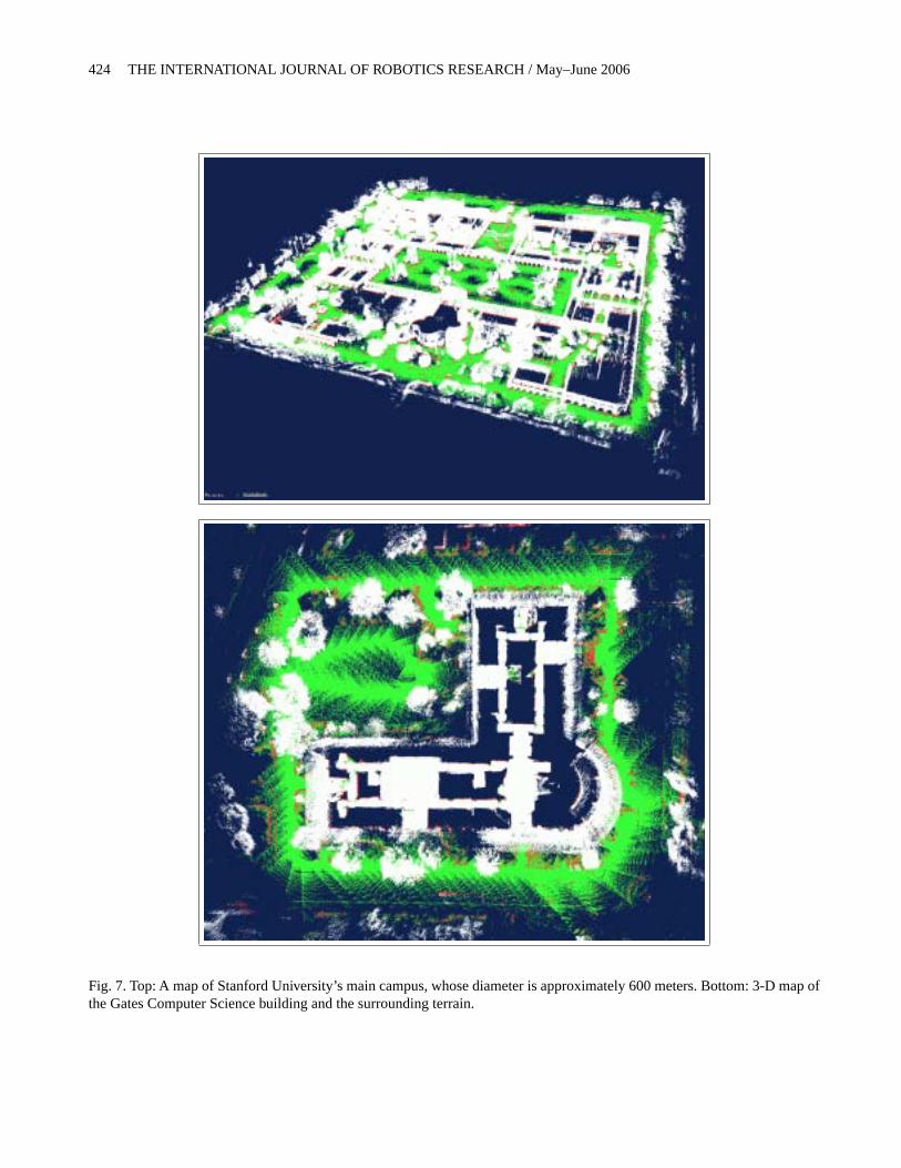
Experimental snapshots can be found in Figures 6through 8. Figures 7 and 8 show some of the maps acquired by
our system. All maps are substantially larger than previouslysoftware could handle, all are constructed with some GPS in-formation. The map shown on the top in Figure 7 correspondsto Stanford’s main campus; the one on the bottom is an indoor-outdoor map of the building that houses the computer sciencedepartment.
The key result of improved indoor maps through combin-ing indoor and outdoor mapping is illustrated in Figure 6. Herewe show 2-D slices of the 3-D map in Figure 7 using SLAMunder two different conditions: In the map on the top, the in-door map is constructed independently of the outdoor map,whereas the bottom map is constructed jointly. As explained,the joint construction lets GPS information affect the buildinginterior through the sequence of potentials liking the outdoorto the indoor. As this figure suggests, the joint indoor-outdoormap is significantly more accurate; in fact, the building pos-sesses a right angle at its center, which is well approximated.
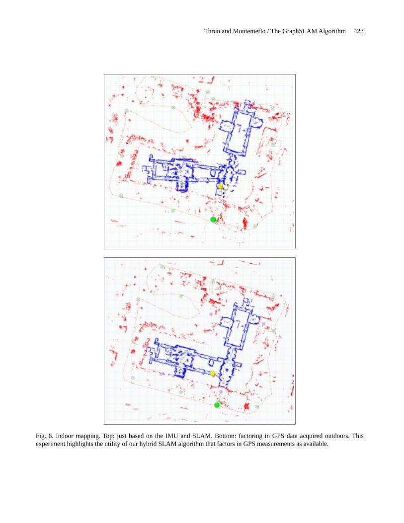
Thrun and Montemerlo / The GraphSLAM Algorithm 423
Fig. 6. Indoor mapping. Top: just based on the IMU and SLAM. Bottom: factoring in GPS data acquired outdoors. Thisexperiment highlights the utility of our hybrid SLAM algorithm that factors in GPS measurements as available.
424 THE INTERNATIONAL JOURNAL OF ROBOTICS RESEARCH / May–June 2006
Fig. 7. Top: A map of Stanford University’s main campus, whose diameter is approximately 600 meters. Bottom: 3-D map ofthe Gates Computer Science building and the surrounding terrain.

Thrun and Montemerlo / The GraphSLAM Algorithm 425
Fig. 8. Visualization of the NASA Ames ARC Disaster Assistance and Rescue Team training site in Moffett Field, CA. Thissite consist of a partially collapsed building with two large observation platforms.
8. Conclusion
We presented the GraphSLAM algorithm, which solves a spe-cific version of the SLAM problem, called the offline problem(or full SLAM problem). The offline problem is characterizedby a feasibility to accumulate all data during mapping, andresolve this data into a map after the robot’s operation is com-plete. GraphSLAM achieves the latter by mapping the datainto a sparse graph of constraints, which are then mappedinto an information form representation using linearizationthrough Taylor expansion. The information form is then re-duced by applying exact transformations, which remove themap variables from the optimization problem. The resultingoptimization problem is solved via a standard optimizationtechnique, such as conjugate gradient. GraphSLAM recoversthe map from the pose estimate, through a sequence of de-coupled small-scale optimization problems (one per feature).Iteration of the linearization and optimization technique yieldsaccurate maps in environments with 108 features or more.
The GraphSLAM algorithm follows a rich tradition of pre-viously published offline SLAM algorithms, which are allbased on the insight that the full SLAM problem corresponds
to a sparse spring-mass system. The key innovation in thispaper is the reduction step, through which the problem of in-ference in this graphical model becomes manageable. Thisstep is essential in achieving scalability in offline SLAM.
Experimental results in large-scale urban environmentsshow that the GraphSLAM approach indeed leads to viablemaps. Our experiments show that it is relatively straightfor-ward to include other information sources—such as GPS—into the SLAM problem, by defining appropriate graphicalconstraints. For example, we were able to show that throughthe graphical model, GPS data acquired outside a build-ing structure could be propagated into the building interior,thereby improving the accuracy of an interior map.
GraphSLAM is characterized by a number of limitations.One arises from the assumption of independent Gaussiannoise. Clearly, real-world noise is not Gaussian and, moreimportantly, it is not independent. We find in practice that thisproblem can be alleviated by artificially increasing the covari-ance of the noise variables, which reduces the informationavailable for SLAM. However, such methods are somewhatad-hoc; see Guivant and Masson (2005) for further treatmentof non-Gaussian noise.
426 THE INTERNATIONAL JOURNAL OF ROBOTICS RESEARCH / May–June 2006
GraphSLAM is also limited in its reliance on a good initialestimate of the map, computed in Table 1.As the total numberof time steps increases, the accuracy of the odometry-basedinitial guess will degrade, leading to an increased number ofdata association errors. GraphSLAM, as formulated in thispaper, will eventually diverge because of this initial pose es-timation step. However, the data set may often be broken intopieces, for which SLAM can be performed individually beforepasting together the total set of constraints. Such a hierarchicalcomputation is subject of future research.
Another limitation pertains to the matrix inversion in Ta-ble 4. This inversion can be painfully slow; and optimizationmethods such as conjugate gradient (as brought to bear in ourexperiments, can be much more efficient.
More broadly, there remain a number of open questionsthat warrant future research. Chief among them is the devel-opment of SLAM techniques that can handle basic buildingelements, such as walls, windows, roofs, and so on. Graph-SLAM makes a static world assumption, and more researchis needed to understand SLAM in dynamic environments (seeHähnel, Schulz, and Burgard 2003; Wang, Thorpe, and Thrun2003 for notable exceptions). Finally, bridging the gap be-tween online and offline SLAM algorithm is a worthwhilegoal of future research.
Appendix: Derivations
The derivations in this section are standard textbook material.
Derivation of the Inversion Lemma
Define� = (Q−1 + P T R−1 P)−1. It suffices to show that
(R−1 − R−1 P � P T R−1) (R + P Q P T ) = I
This is shown through a series of transformations:
= R−1 R︸ ︷︷ ︸= I
+ R−1 P Q P T − R−1 P � P T R−1 R︸ ︷︷ ︸= I
− R−1 P � P T R−1 P Q P T
= I + R−1 P Q P T − R−1 P � P T
− R−1 P � P T R−1 P Q P T
= I + R−1 P [Q P T
−� P T − � P T R−1 P Q P T ]= I + R−1 P [Q P T − � Q−1 Q︸ ︷︷ ︸
= I
P T
−� P T R−1 P Q P T ]= I + R−1 P [Q P T − � �−1︸ ︷︷ ︸
= I
Q P T ]
= I + R−1 P [Q P T − Q P T︸ ︷︷ ︸= 0
] = I
Marginals of a Multivariate Gaussian
The marginal for a Gaussian in its moments parameterization
� =(
�xx �xy
�yx �yy
)and µ =
(µx
µy
)
is N (µx, �xx). By definition, the information matrix of thisGaussian is therefore�−1
xx, and the information vector is
�−1xx
µx . We show�−1xx= �xx via the Inversion Lemma from
Table 6; this derivation makes the assumption that none of theparticipating matrices is singular. LetP = (0 1)T , and let[∞] be a matrix of the same size as�yy but whose entries areall infinite (and with[∞]−1 = 0. This gives us
(�+ P [∞]P T )−1 =(
�xx �xy
�yx [∞])−1
(∗)=(
�−1xx
00 0
)
The same expression can also be expanded by the inversionlemma into:
(�+ P [∞]P T )−1
= �−� P([∞]−1 + P T � P)−1 P T �
= �−� P(0+ P T � P)−1 P T �
= �−� P(�yy)−1 P T �
=(
�xx �xy
�yx �yy
)−(
�xx �xy
�yx �yy
)(0 00 �−1
yy
)(
�xx �xy
�yx �yy
)(∗)=
(�xx �xy
�yx �yy
)−(
0 �xy �−1yy
0 1
)(�xx �xy
�yx �yy
)
=(
�xx �xy
�yx �yy
)−(
�xy �−1yy
�yx �xy
�yx �yy
)
=(
�xx 00 0
)
The remaining statement,�−1xx
µx = ξx , is obtained analo-gously, exploiting the fact thatµ = �−1ξ and the equality ofthe two expressions marked “(∗)” above:(
�−1xx
µx
0
)=
(�−1
xx0
0 0
)(µx
µy
)
=(
�−1xx
00 0
)�−1
(ξx
ξy
)(∗)=
[�−
(0 �xy �−1
yy
0 1
)�
]�−1
(ξx
ξy
)
=(
ξx
ξy
)−(
0 �xy �−1yy
0 1
)(ξx
ξy
)
=(
ξx
0
)

Thrun and Montemerlo / The GraphSLAM Algorithm 427
Conditionals of a multivariate Gaussian
Proof. The result follows trivially from the definition of aGaussian in information form:
p(x | y)
= η exp
{−1
2
(x
y
)T (�xx �xy
�yx �yy
)(x
y
)
+(
x
y
)T (ξx
ξy
)}
= η exp
{−1
2xT �xxx + xT �xyy − 1
2
+yT �yyy + xT ξx + yT ξy
}= η exp{−1
2xT �xxx
+xT (�xyy + ξx)−1
2+ yT �yyy + yT ξy︸ ︷︷ ︸
const.
}
= η exp{−1
2xT �xxx + xT (�xyy + ξx)}
References
Allen, P. and Stamos, I. 2000. Integration of range and imagesensing for photorealistic 3D modeling. InProceedings ofthe IEEE International Conference on Robotics and Au-tomation (ICRA), pp. 1435–1440.
Araneda, A. 2003. Statistical inference in mapping and local-ization for a mobile robot. InBayesian Statistics 7. (edsBernardo, J. M., Bayarri, M., Berger, J., Dawid, A. P.,Heckerman, D., Smith, A., and West, M). Oxford Univer-sity Press, Oxford, UK.
Bailey, T. 2002.Mobile Robot Localisation and Mapping inExtensive Outdoor Environments. PhD thesis, Universityof Sydney, Sydney, NSW, Australia.
Bajcsy, R., Kamberova, G., and Nocera, L. 2000. 3D re-construction of environments for virtual reconstruction. InProc. of the 4th IEEE Workshop on Applications of Com-puter Vision.
Baker, C., Morris, A., Ferguson, D., Thayer, S., Whittaker,C., Omohundro, Z., Reverte, C., Whittaker, W., Hähnel,D., and Thrun, S. 2004. A campaign in autonomous minemapping. InProceedings of the IEEE International Con-ference on Robotics and Automation (ICRA).
Bosse, M., Newman, P., Leonard, J., Soika, M., Feiten, W.,and Teller, S. 2004. Simultaneous localization and mapbuilding in large-scale cyclic environments using the at-las framework.International Journal of Robotics Research23(12):1113–1139.
Bosse, M., Newman, P., Soika, M., Feiten,W., Leonard, J., andTeller, S. 2003. An atlas framework for scalable mapping.
In Proceedings of the IEEE International Conference onRobotics and Automation (ICRA).
Bulata, H. and Devy, M. 1996. Incremental construction of alandmark-based and topological model of indoor environ-ments by a mobile robot. InProceedings of the IEEE Inter-national Conference on Robotics and Automation (ICRA),Minneapolis, USA.
Cheeseman, P. and Smith, P. 1986. On the representation andestimation of spatial uncertainty.International Journal ofRobotics 5:56–68.
Cowell, R., Dawid, A., Lauritzen, S., and Spiegelhalter,D. 1999. Probabilistic Networks and Expert Systems.Springer Verlag, Berlin, New York.
Csorba, M. 1997.Simultaneous Localisation and Map Build-ing. PhD thesis, University of Oxford.
Dissanayake, G., Newman, P., Clark, S., Durrant-Whyte, H.,and Csorba, M. 2001.A solution to the simultaneous local-isation and map building (SLAM) problem.IEEE Trans-actions of Robotics and Automation 17(3):229–241.
Duckett,T., Marsland, S., and Shapiro, J. 2000. Learning glob-ally consistent maps by relaxation. InProceedings of theIEEE International Conference on Robotics and Automa-tion, San Francisco, pp. 3841–3846.
Duckett, T., Marsland, S., and Shapiro, J. 2002. Fast, on-linelearning of globally consistent maps.Autonomous Robots12(3):287–300.
Durrant-Whyte, H. 1988. Uncertain geometry in robotics.IEEE Transactions on Robotics and Automation 4(1):23–31.
El-Hakim, S., Boulanger, P., Blais, F., and Beraldin, J.-A. 1997.Sensor based creation of indoor virtual environment mod-els. InProc. of the 4th Internetional Conference on VirtualSystems and Multimedia (VSMM), Geneva, Switzerland.
Elfes, A. 1987. Sonar-based real-world mapping and navi-gation. IEEE Journal of Robotics and Automation RA-3(3):249–265.
Folkesson, J. and Christensen, H. I. 2004a. Graphical SLAM:A self-correcting map. InProceedings of the IEEE Inter-national Conference on Robotics and Automation (ICRA),New Orleans, USA.
Folkesson, J. and Christensen, H. I. 2004b. Robust SLAM.In Proceedings of the International Symposium on Au-tonomous Vehicles, Lisboa, PT.
Frese, U. 2004.An O(logn) Algorithm for Simultaneous Lo-calization and Mapping of Mobile Robots in Indoor En-vironments. PhD thesis, University of Erlangen-Nürnberg,Germany.
Frese, U. and Hirzinger, G. 2001. Simultaneous localizationand mapping—a discussion. InProceedings of the IJCAIWorkshop on Reasoning with Uncertainty in Robotics, pp.17–26, Seattle, WA.
Frese, U., Larsson, P., and Duckett, T. 2005. A Multigrid Al-gorithm for Simultaneous Localization and Mapping. InIEEE Transactions on Robotics, 21(2):1-12.

428 THE INTERNATIONAL JOURNAL OF ROBOTICS RESEARCH / May–June 2006
Golfarelli, M., Maio, D., and Rizzi, S. 1998. Elastic correc-tion of dead-reckoning errors in map building. InProceed-ings of the IEEE/RSJ International Conference on Intel-ligent Robots and Systems (IROS), pp. 905–911, Victoria,Canada.
Guivant, J. and Masson, F. 2005. Using absolute non-gaussiannon-white observations in Gaussian SLAM. InProceed-ings of the IEEE International Conference on Roboticsand Automation (ICRA), Barcelona, Spain.
Guivant, J. and Nebot, E. 2001. Optimization of the simul-taneous localization and map building algorithm for realtime implementation.IEEE Transactions of Robotics andAutomation 17(3):242–257.
Gutmann, J.-S. and Konolige, K. 2000. Incremental mappingof large cyclic environments. InProceedings of the IEEEInternational Symposium on Computational Intelligencein Robotics and Automation (CIRA).
Gutmann, J.-S. and Nebel, B. 1997. Navigation mobilerroboter mit laserscans. InAutonome Mobile Systeme.Springer Verlag, Berlin. In German.
Hähnel, D., Burgard, W., Wegbreit, B., and Thrun, S. 2003a.Towards lazy data association in SLAM. InProceedingsof the 11th International Symposium of Robotics Research(ISRR’03), Sienna, Italy. Springer.
Hähnel, D., Schulz, D., and Burgard, W. 2003b. Mobile robotmapping in populated environments.Autonomous Robots17(7):579–598.
Iocchi, L., Konolige, K., and Bajracharya, M. 2000. Visuallyrealistic mapping of a planar environment with stereo. InProceesings of the 2000 International Symposium on Ex-perimental Robotics, Waikiki, Hawaii.
Julier, S. and Uhlmann, J. K. 2000. Building a million bea-con map. InProceedings of the SPIE Sensor Fusion andDecentralized Control in Robotic Systems IV, Vol. #4571.
Konecny, G. 2002.Geoinformation: Remote Sensing, Pho-togrammetry and Geographical Information Systems. Tay-lor & Francis.
Konolige, K. 2004. Large-scale map-making. InProceedingsof the AAAI National Conference on Artificial Intelligence,pp. 457–463, San Jose, CA. AAAI.
Kuipers, B., Modayil, J., Beeson, P., MacMahon, M., andSavelli, F. 2004. Local metrical and global topologicalmaps in the hybrid spatial semantic hierarchy. InProceed-ings of the IEEE International Conference on Robotics andAutomation (ICRA), New Orleans.
Lawler, E. and Wood, D. 1966. Branch-and-bound methods:A survey.Operations Research 14:699–719.
Leonard, J. J. and Durrant-Whyte, H. F. 1991. Mobile robotlocalization by tracking geometric beacons.IEEE Trans-actions on Robotics and Automation 7(3):376–382.
Leonard, J. and Newman, P. 2003. Consistent, convergent, andconstant-time SLAM. InProceedings of the IJCAI Work-shop on Reasoning with Uncertainty in Robot Navigation,Acapulco, Mexico.
Leonard, J., Tardós, J., Thrun, S., and Choset, H. (eds) 2002.Workshop Notes of the ICRA Workshop on ConcurrentMapping and Localization for Autonomous Mobile Robots(W4). ICRA Conference, Washington, DC.
Levoy, M. 1999. The digital michelangelo project. InProc. ofthe Second International Conference on 3D Imaging andModeling.
Liu, Y. and Thrun, S. 2003. Results for outdoor-SLAM usingsparse extended information filters. InProceedings of theIEEE International Conference on Robotics and Automa-tion (ICRA).
Lu, F. and Milios, E. 1997. Globally consistent range scanalignment for environment mapping.Autonomous Robots4:333–349.
Montemerlo, M., Roy, N., and Thrun, S. 2003. Perspec-tives on standardization in mobile robot programming:The Carnegie Mellon navigation (CARMEN) toolkit.In Proceedings of the Conference on Intelligent Robotsand Systems (IROS). Software package for download atwww.cs.cmu.edu/∼carmen.
Montemerlo, M. and Thrun, S. 2004. Large-scale robotic 3-d mapping of urban structures. InProceedings of the In-ternational Symposium on Experimental Robotics (ISER),Singapore. Springer Tracts inAdvanced Robotics (STAR).
Montemerlo, M., Thrun, S., Koller, D., andWegbreit, B. 2002.FastSLAM: A factored solution to the simultaneous local-ization and mapping problem. InProceedings of the AAAINational Conference on Artificial Intelligence, Edmonton,Canada. AAAI.
Moravec, H. P. 1988. Sensor fusion in certainty grids for mo-bile robots.AI Magazine 9(2):61–74.
Moutarlier, P. and Chatila, R. 1989a. An experimental systemfor incremental environment modeling by an autonomousmobile robot. In1st International Symposium on Experi-mental Robotics, Montreal.
Moutarlier, P. and Chatila, R. 1989b. Stochastic multisensorydata fusion for mobile robot location and environmentmodeling. In5th Int. Symposium on Robotics Research,Tokyo.
Narendra, P. and Fukunaga, K. 1977. A branch and boundalgorithm for feature subset selection.IEEE Transactionson Computers 26(9):914–922.
Newman, P. 2000.On the Structure and Solution of the Si-multaneous Localisation and Map Building Problem. PhDthesis, Australian Centre for Field Robotics, University ofSydney, Sydney, Australia.
Newman, P. M. and Durrant-Whyte, H. F. 2001. A new solu-tion to the simultaneous and map building (SLAM) prob-lem. InProceedings of SPIE.
Newman, P. and Rikoski, J. L. R. 2003. Towards constant-timeslam on an autonomous underwater vehicle using syntheticaperture sonar. InProceedings of the International Sympo-sium of Robotics Research, Sienna, Italy.
Paskin, M. 2003. Thin junction tree filters for simultaneous

Thrun and Montemerlo / The GraphSLAM Algorithm 429
localization and mapping. InProceedings of the SixteenthInternational Joint Conference on Artificial Intelligence(IJCAI), Acapulco, Mexico. IJCAI.
Pearl, J. 1988.Probabilistic reasoning in intelligent systems:networks of plausible inference. Morgan Kaufmann Pub-lishers, San Mateo, CA.
Pollefeys, M., Koch, R., and Gool, L.V. 1998. Self-calibrationand metric reconstruction in spite of varying and unknowninternal camera parameters. InProceedings of the Interna-tional Conference on Computer Vision, pp. 90–95, Bom-bay, India. IEEE.
Rusinkiewicz, S. and Levoy, M. 2001. Efficient variants of theICP algorithm. InProc. Third International Conference on3D Digital Imaging and Modeling (3DIM), Quebec City,Canada. IEEEComputer Society.
Smith, R. and Cheeseman, P. 1986. On the representation andestimation of spatial uncertainty.International Journal ofRobotics Research 5(4):56–68.
Smith, R., Self, M., and Cheeseman, P. 1990. Estimating un-certain spatial relationships in robotics. InAutonomousRobot Vehicles (eds Cox, I. and Wilfong, G.) pp. 167–193.Springer-Verlag.
Soatto, S. and Brockett, R. 1998. Optimal structure from mo-tion: Local ambiguities and global estimates. InProceed-ings of the Conference on Computer Vision and PatternRecognition (CVPR), pp. 282–288.
Tardós, J., Neira, J., Newman, P., and Leonard, J. 2002. Ro-bust mapping and localization in indoor environments us-ing sonar data.International Journal of Robotics Research21(4):311–330.
Teller, S., Antone, M., Bodnar, Z., Bosse, M., Coorg, S.,Jethwa, M., and Master, N. 2001. Calibrated, registeredimages of an extended urban area. InProceedings of the
Conference on Computer Vision and Pattern Recognition(CVPR).
Thrun, S., Koller, D., Ghahramani, Z., Durrant-Whyte, H., andNg, A. 2002. Simultaneous mapping and localization withsparse extended information filters. InProceedings of theFifth International Workshop on Algorithmic Foundationsof Robotics (eds Boissonnat, J.-D., Burdick, J., Goldberg,K., and Hutchinson, S.), Nice, France.
Thrun, S. and Liu, Y. 2003. Multi-robot SLAM with sparseextended information filers. InProceedings of the 11th In-ternational Symposium of Robotics Research (ISRR’03),Sienna, Italy. Springer.
Tomasi, C. and Kanade, T. 1992. Shape and motion from im-age streams under orthography: A factorization method.International Journal of Computer Vision 9(2):137–154.
Uhlmann, J., Lanzagorta, M., and Julier, S. 1999. The NASAmars rover:A testbed for evaluating applications of covari-ance intersection. InProceedings of the SPIE 13th AnnualSymposium in Aerospace/Defence Sensing, Simulation andControls.
Wang, C.-C., Thorpe, C., and Thrun, S. 2003. Online simulta-neous localization and mapping with detection and track-ing of moving objects: Theory and results from a groundvehicle in crowded urban areas. InProceedings of theIEEE International Conference on Robotics and Automa-tion (ICRA).
Williams, S. B. 2001.Efficient Solutions to Autonomous Map-ping and Navigation Problems. PhD thesis,ACFR, Univer-sity of Sydney, Sydney, Australia.
Williams, S., Dissanayake, G., and Durrant-Whyte, H. 2001.Towards terrain-aided navigation for underwater robotics.Advanced Robotics 15(5).