the graph isomorphism problem and the structure …the graph isomorphism problem and the structure...
TRANSCRIPT

The graph isomorphismproblem and the structure of
walks
Peter MadarasiApplied Mathematics MSc
Thesis
Supervisor:Alpar Juttner
senior research fellowELTE Institute of Mathematics,
Department of Operations Research
Eotvos Lorand UniversityFaculty of Science
Budapest, 2018

Contents
1 Introduction 4
2 Preliminaries 8
2.1 Notation . . . . . . . . . . . . . . . . . . . . . . . . . . . . . . 8
2.2 Linear algebra . . . . . . . . . . . . . . . . . . . . . . . . . . . 9
2.3 Hashing . . . . . . . . . . . . . . . . . . . . . . . . . . . . . . 10
3 Artificial labels 11
3.1 Walk-labeling . . . . . . . . . . . . . . . . . . . . . . . . . . . 12
3.1.1 Getting rid of infinite labels . . . . . . . . . . . . . . . 13
3.1.2 Walk labels in practice . . . . . . . . . . . . . . . . . . 15
3.2 Strong walk-labeling . . . . . . . . . . . . . . . . . . . . . . . 17
3.2.1 Strong walk labels in practice . . . . . . . . . . . . . . 19
4 Some theoretical results 20
4.1 Walk-labeling . . . . . . . . . . . . . . . . . . . . . . . . . . . 21
4.2 Strong walk-labeling . . . . . . . . . . . . . . . . . . . . . . . 28
4.3 Polynomial time graph isomorphism algorithm for certain graphclasses . . . . . . . . . . . . . . . . . . . . . . . . . . . . . . . 30
5 Applications 32
5.1 Node-labeling . . . . . . . . . . . . . . . . . . . . . . . . . . . 32
5.1.1 Biological graphs . . . . . . . . . . . . . . . . . . . . . 33
5.1.2 Regular graphs . . . . . . . . . . . . . . . . . . . . . . 36
5.2 A sophisticated backtracking algorithm . . . . . . . . . . . . . 39
5.3 The (induced) subgraph isomorphism problem . . . . . . . . . 40
1

5.4 Graph fingerprints . . . . . . . . . . . . . . . . . . . . . . . . 41
5.4.1 Strong walk fingerprint . . . . . . . . . . . . . . . . . 42
5.4.2 Walk fingerprint . . . . . . . . . . . . . . . . . . . . . . 43
5.4.3 Generalization of strong walk fingerprint . . . . . . . . 44
6 Conclusion and future work 44
7 Acknowledgement 45
2

Abstract
This thesis presents the concept of walk-labeling that can be used tosolve the graph isomorphism problem in polynomial time combinatoriallyunder certain conditions — which hold for a wide range of the graph pairs.It turns out that all non-cospectral graph pairs can be differentiated with acombinatorial method, furthermore, even non-isomorphic co-spectral graphsmight be distinguished by combinatorially verifying certain properties of theireigenspaces. New polynomial time graph isomorphism algorithms are givenunder certain spectral conditions and in the case of large graph diameter.
The concept of strong walk-labeling is a refinement of the aforemen-tioned labeling, which has important theoretical and practical applications.Its applications include speeding up any backtracking graph matching al-gorithm, and the generation of graph fingerprints, which uniquely identifyall the graphs in the considered databases — including all strongly regulargraphs on at most 64 vertices. They are also proved to identify all trees up toisomorphism, which — as a byproduct — gives a new isomorphism algorithmfor trees. The practical importance of this fingerprint lies in significantlyspeeding up searching in graph databases and graph matching algorithms,which are commonly required in biological and chemical applications.
In addition to the theoretical results, computational tests have beencarried out on biological, strongly regular and random graphs to practicallyevaluate the proposed methods.
3

1 Introduction
In the last decades, combinatorial structures and especially graphs havebeen considered with ever increasing interest, and applied to the solution ofseveral new and revised questions. The expressiveness, the simplicity andthe deep theoretical background of graphs make it one of the most usefulmodeling tool, which appears constantly in several seemingly independentfields, such as bioinformatics and chemistry.
Getting acquainted with the structure of complex biological systems atthe molecular level is of primary importance, since protein-protein inter-action, DNA-protein interaction, metabolic interaction, transcription factorbinding, neuronal networks, and hormone singling networks may be betterunderstood this way.
Many chemical and biological structures can easily be modeled this way,for instance, a molecular structure can be considered as a graph, whose nodesand edges correspond to atoms and chemical bonds, respectively. The sim-ilarity and dissimilarity of objects corresponding to nodes may be incorpo-rated to the model by node labels. Understanding such networks basicallyrequires finding specific subgraphs, thus it calls for efficient graph matchingalgorithms.
Other real-world fields related to some variants of graph matching in-clude pattern recognition and machine vision [7], symbol recognition [12],and face identification [20].
While this work focuses on the graph isomorphism problem in the firstplace, some of the proposed methods can be applied in the case of subgraphand induces subgraph matching problems, as well.
Subgraph and induced subgraph matching problems are known to beNP-Complete [9], while the graph isomorphism problem is one of the prob-lems in NP neither known to be in P nor NP-Complete. At the sametime, polynomial-time isomorphism algorithms are known for various graphclasses, like trees and planar graphs [17], bounded valence graphs [22], inter-val graphs [21] or permutation graphs [8]. Furthermore, an FPT algorithmhas also been recently presented for the colored hypergraph isomorphismproblem in [2].
4

Some algorithms which do not need any restrictions on the graphs aresummarized below. Even though, an overall polynomial behavior may notbe expected from such an alternative, they may often have good practicalperformance. In fact, they might be the best choice in practice even on agraph class for which polynomial algorithm is known.
The first practically efficient approach was due to Ullmann [33], whichis a commonly used algorithm based on depth-first search with a complexheuristic for reducing the number of visited states. A major problem is itsΘ(n3) space complexity, which makes it impractical for big sparse graphs. Ina recent paper, Ullmann [18] presents an improved version of this algorithmbased on a bit-vector solution for the binary Constraint Satisfaction Problem.
The Nauty algorithm [25] transforms the two graphs to a canonical formbefore starting to look for an isomorphism. It has been considered as oneof the fastest graph isomorphism algorithms, although graph categories wereshown in which it takes exponentially many steps. This algorithm handlesonly the graph isomorphism problem.
The LAD algorithm [31] uses a depth-first search strategy and formulatesthe matching as a Constraint Satisfaction Problem to prune the search tree.The constraints are that the mapping has to be injective and edge-preserving,hence it is possible to handle new matching types as well.
The RI algorithm [5] and its variations are based on a state space rep-resentation. After reordering the nodes of the graphs, it uses some fast toexecute heuristic checks without using any complex pruning rules. It seemsto run really efficiently on graphs coming from biology, and won the Inter-national Contest on Pattern Search in Biological Databases [35].
Currently, one of the most commonly used algorithm is VF2 [11], an im-proved version of VF [10], which was designed for solving pattern matchingand computer vision problems, and has been one of the best overall algo-rithms for more than a decade. Although, it is not as fast as some of thenew specialized algorithms, it is still widely used due to its simplicity andspace efficiency. VF2 uses a state space representation and checks specificconditions in each state to prune the search tree.
Another variant called VF2++ [19],[23] has recently been published.It is one of the most efficient graph matching algorithms on biological and
5
chemical graph. This method is at least as efficient as the RI or other VF2-like methods, and it has strictly better behavior on large graphs. The mainidea of VF2++ is to precompute a heuristic node order of the graph to beembedded, on which VF2 works more efficiently, and apply stronger cuttingrules - which are easier to verify at the same time.
In addition to checking whether two given graphs are (sub)graph iso-morphic, in many cases a given graph G is searched in a database. Insteadof solving the graph isomorphism problem for G and for each graphs in thedatabase, one might generate so called fingerprints for all graphs s.t. if twofingerprints are different, then the corresponding graphs can not be isomor-phic. Now, one has to solve the graph isomorphism problem only for graphshaving the same fingerprint as G does.
Graph fingerprints are widely used, and several schemes have been pro-posed to generate them. In [30], graph fingerprints were generated by consid-ering the node labels of short paths. This type of fingerprints is also usefulin the case of subgraph matching.
Fingerprints constructed by combining the Laplacian spectrum and theheat kernels associated to the graph Laplacian is described in [27]. In general,the strength of graph spectrum as signature is theoretically studied in [34]and [36]. The developed tool apparently works only for graph having specialstructures, such as distance-regular graphs. They conclude that it seems tobe out of reach to answer which graphs are determined by their adjacencyand Laplacian spectrum. However, the number of graphs determined by theirspectrum was numerically examined up to 12 nodes in [15], and around 80%of the graphs were found to be determined by their spectrum. Note that itis conjectured that almost all graphs are determined by their spectrum.
Recently, various algorithms have been developed based on discrete timequantum walks (DTQW) or continuous time quantum walks (CTQW), aim-ing at distinguishing non-isomorphic graph pairs. It is well known thatneither standard single-particle DTQW nor CTQW can distinguish a pairof Strongly regular graphs (SRG) of the same parameters, furthermore aconstant-particle CTQW without interaction can distinguish no SRG pairsof the same parameters, see [14] and [28]. However, the distinguishing
6

power of a variant of single-particle DTQW presented in [14] turned out tobe larger than that of a standard DTQW. Namely, it generates different sig-natures for certain non-isomorphic SRG pairs of the same parameters, butthere are SRG pairs that it fails to distinguish. In [24], CTQW were shown tobe less powerful than DTQW as far as the graph isomorphism is concerned.
On the other hand, a state-of-the-art quantum walk method using in-teracting bosons turned out to distinguish all SRG’s on at most 64 vertices[16]. In this light, it is especially precious that the fingerprint introduced inSection 5 distinguishes all the mentioned SRG’s, in addition, it provides acompact description of the graphs.
This work presents the concept of walk-labeling, which can be used tosolve the graph isomorphism problem combinatorially in polynomial time un-der certain conditions - which hold for a wide range of the graph pairs. Allnon-cospectral graph pairs are proved to be distinguished by the proposedcombinatorial method (without computing the graph spectra). Furthermore,even if the graphs are cospectral and non-isomorphic, various conditions areshown to ensure that the graphs are distinguished. Polynomial time isomor-phism algorithm will be given for graphs of large diameter.
For practical purposes, a refinement of the aforementioned labeling calledstrong walk-labeling is also introduced. Its applications include speedingup any backtracking-based graph matching algorithm, which will be testedby counting the number of backtracks the VF2 algorithm takes on differ-ent graph classes. Another important application is a fingerprint generationmethod based on strong walk-labeling, which was able to uniquely identifyall the graphs in the considered graph databases — including all the knownstrongly regular graphs. Therefore, it is competitive with the state-of-the-artquantum walk algorithms and compress all information about the graph ina short fingerprint, as well. Note that the strongly regular graphs are wellknown as possibly the hardest instances of the graph isomorphism problem.
The rest of the thesis is structured as follows. Section 2 introducesthe most important notations and results that will be used throughout thiswork. Section 3 defines the artificial labels, the fundamental concept of thiswork. Theoretical results demonstrating the strength of the proposed artifi-
7

cial labels are described in Section 4. The most important applications arepresented in Section 5, including the generation of unique graph identifiers.The thesis is concluded by a brief summary of the open questions.
2 Preliminaries
This section introduces the notations, and some of the main results thatwill be used throughout this thesis.
2.1 Notation
As usual, sets are described in curly brackets, and multisets are describedin curly brackets followed by a superscript hash character. For example,{1, 2, 3} denotes the set consisting of the numbers 1,2,3, and {1, 1, 2, 3}#
denotes the multiset consisting of numbers 1,1,2,3.
Let N denote the non-negative integer numbers.
For a positive integer n, let [n] denote the set {i ∈ N : 1 ≤ i ≤ n}.
Throughout the thesis G = (V,E), G1 = (V1, E1) and G2 = (V2, E2)denote three arbitrary loop-free undirected graphs with n > 1 nodes, whereV, V1, V2 denotes the node sets and E,E1, E2 the edge sets, respectively. Forthe sake of simplicity, the node sets are assumed to be [n], that is V = V1 =V2 = [n]. The adjacency matrices of these graphs are A,A1, A2 ∈ {0, 1}n×n,respectively.
Unless stated otherwise, the presented results apply to graphs havingloops, as well. Note that node labeled graphs can be modeled by addingloops, and clearly, even if the graph has both loops and node labels, there isa compact way to encode them using loops only. Therefore node labels canbe omitted likewise.
Let ΓG(i) denote the set of the neighbors of node i in graph G.
Finally, let δij =
1, if i = j
0, otherwisedenote the Kronecker delta.
8

2.2 Linear algebra
For later reference, some of the well-known results in linear algebra aresummarized here.
Theorem 2.2.1. The adjacency matrix of a graph has n eigenvalues over R.
Theorem 2.2.2. Let G be a simple graph with adjacency matrix A, and letλ1 ≥ λ2 ≥ .. ≥ λn denote the eigenvalues of A. There are u1, .., un ∈ Rn
orthonormal eigenvectors s.t. Aui = λiui for all i ∈ [n].
The adjacency matrices of G1 and G2 are denoted by A1 and A2, respec-tively. Let λ1 ≥ λ2 ≥ .. ≥ λn and µ1 ≥ µ2 ≥ .. ≥ µn denote their eigenvalues.G1 and G2 are cospectral if the multisets of the eigenvalues of A1 and A2 arethe same, that is {λi : i ∈ [n]}# = {µi : i ∈ [n]}#. Let U, V ∈ Rn×n orthog-onal matrices (i.e. UTU = I and V TV = I) s.t. A1U = U diag(λ1, λ2, .., λn)and A2V = V diag(µ1, µ2, .., µn). U and V are called the eigenmatrices ofG1 and G2, respectively. Let u1, u2, ..un and v1, v2, ..vn denote the columnvectors of U and V , respectively.
Note that V denotes both the eigenmatrix of G2 and the node set of G,but this will not cause ambiguity.
Please note that uij denotes the jth entry of eigenvector ui, i.e. it is theentry of U in the jth row and ith column, where i, j ∈ [n]. Similarly, vij = Vjifor i, j ∈ [n].
Theorem 2.2.3. The minimal polynomial of a real symmetric matrix A ismA(x) =
p∏i=1
(x− λi), where λ1, λ2, ..λp are the distinct eigenvalues of A.
Theorem 2.2.4 (Perron-Frobenius). If a real square matrix has nonnegativeentries, then it has a nonnegative real eigenvalue λ which has maximumabsolute value among all eigenvalues. This eigenvalue has a nonnegative realeigenvector. If, in addition, the matrix does not contain a k×(n−k) block of0-s disjoint from the diagonal, then λ has multiplicity 1 and the correspondingeigenvector can be chosen positive.
The following theorem is an immediate consequence of Theorem 2.2.4.
9

Theorem 2.2.5. Graph G is connected and has at least two nodes. Thelargest eigenvalue of the adjacency matrix of G is positive and has multiplicityone.
The positive normalized eigenvector corresponding to the largest positiveeigenvalue in Theorem 2.2.5 will be referred to as the Perron-Frobeniuseigenvector of G.
The following lemma and its corollary will play fundamental role in theproofs of the theoretical results presented in Section 4.
Lemma 2.2.6. For all i, j ∈ [n] and for all l ≥ 1, (Al)ij =n∑k=1
ukiukjλlk
holds, where λ1, λ2, ..λn are the eigenvalues of G. The right-hand side of thisequation will be referred to as the eigen decomposition.
Proof: U ∈ Rn×n is an orthonormal matrix s.t. AU = U diag(λ1, λ2, ..λn).Clearly, U−1AlU = diag(λl1, λl2, ..λln) holds, henceAl = U diag(λl1, λl2, ..λln)U−1.Therefore, (Al)ij =
n∑k=1
ukiukjλlk for any node pair i, j ∈ [n].
The following observation is an immediate consequence of Lemma 2.2.6.
Corollary 2.2.7. For all i, j ∈ [n] and l ≥ 1, there exist βij1 , βij2 , ..βijp ∈ R s.t.(Al)ij =
p∑m=1
βijmλlm, where λ1, λ2, ..λp are the distinct non-zero eigenvalues
of G. The the right-hand side of this equation will be referred to as theaggregated eigen decomposition.
Proof: By Lemma 2.2.6, (Al)ij =n∑k=1
ukiukjλlk for l ≥ 1 and i, j ∈ [n].
Clearly, βijm := ∑k:λk=λm
ukiukj is a proper choice, where i, j ∈ [n] and m ∈
[p].
2.3 Hashing
A functionH mapping bitsequences to a set UH is called hash function.By definition, if H(b1) 6= H(b2), then b1 6= b2 for all bitsequences b1, b2. Thepoint is that there are hash functions that (practically) satisfy the other
10
direction, and at the same time, UH is efficient to work with — even if thenthe original bitsequences are exponentially long.
Assume that UH is the set of all bitsequences of length c for a givenconstant c ∈ N, unless otherwise stated.
For a multiset S ⊆ UH, let H(S) denote the bitsequence H(bS), wherebS denotes the bitsequence gained by concatenating the bitsequences of setS in non-decreasing order (bS is of length c|S|). Let H(a1, a2) denote H(b12),where a1 and a2 are s.t. H(a1) and H(a2) are defined, and b12 is the concate-nation of H(a1) and H(a2) in this order.
Note that long bitsequences are mapped to short bitsequences, yet theinjectivity of the function is required. However contradictory this seems, hugepractical experience shows that the SHA512 function fulfills this requirement.On one hand, the incidental hashing errors will not influence the exactnessof the proposed methods, on the other hand, a perfect hash function will bedeveloped later for the specific applications.
3 Artificial labels
This section introduces a concept to classify the nodes of graphs byassigning different labels to them such that if two nodes can be assigned toeach other in an isomorphism, then the assigned labels are equal. The aim isto find node-labelings for which the reverse direction (practically) holds, aswell, i.e. if the labels of two nodes are equal, then there is an isomorphismassigning them to each other.
Definition 3.0.1. A function lG : VG −→ L is called node-labeling, whereG is a graph and L denotes the set of labels.
Definition 3.0.2. A family {lG : G graph} of node-labelings is called ar-tificial labeling if the following holds for all G1, G2 graphs. If there ex-ist an isomorphism mapping node i to node i′, then lG1(i) = lG2(i′) for alli ∈ V1, i
′ ∈ V2.
Three simple examples are shown to demonstrate the concept of artificial
11

labeling. The first example shows that assigning to each node its degree isan artificial labeling.
Example 3.0.1. Let L1 = {l1G : VG −→ N | G graph} a family of node-labelings, where l1G(v) = degG(v), (v ∈ VG).
The following examples strengthen the previous one.
Example 3.0.2. Let L2 = {l2G : VG −→ N | G graph} a family of node-labelings, where l2G(v) = deg(v) + ∑
w∈Γ(v)degG(v), (v ∈ VG).
Example 3.0.3. Let L3 = {l3G : VG −→ (N × 2N) | G graph} a family ofnode labels, where l3G(v) = (deg(v), {deg(w) : w ∈ Γ(v)}), (v ∈ VG).
Observe that the artificial labelings given in the previous examples arenot very strong in the sense that they assign the same label to any two nodesof a d-regular graph.
The following two sections describe two efficient artificial labelings, themain concepts of this work.
3.1 Walk-labeling
This section introduces a special artificial labeling called walk-labeling.
Let Lw = {Q : Q ∈ Nn×N} be the set of labels, i.e. Lw consists ofmatrices having n rows and infinitely many columns. Two such labels, Q1
andQ2 ∈ Lw are said to be permutation-equal if there exists a permutationmatrix P for which PQ1 = Q2. This relation is denoted by Q1
p= Q2.
Claim 3.1.1. p= is an equivalence relation.
The following artificial labeling, besides its practical relevance, playsa primary role when analysing the so-called strong walk-labeling, see Sec-tion 3.2.
Notation 3.1.1. Let `G : VG −→ Nn×N be s.t. `G(i)jl denotes the numberof walks of length l between node i and node j for l ≥ 0. In other words,the lth column of matrix `G(i) is Al−1ei, where ei is the incidence vector ofnode i ∈ VG and l ≥ 1. The function `G will be referred to as (infinite)walk-labeling.
12

The following claim easily follows from the definition of the walk-labeling.
Claim 3.1.2. The family {`G | G graph} is an artificial labeling if labels arecompared using p=.
The definition of walk-isomorphism follows, which plays an importantrole in the studies of Section 4.
Definition 3.1.1. G1 and G2 are walk-isomorphic if the nodes can berelabeled s.t. `G1(i) p= `G2(i) for all node i.
Claim 3.1.3. If two graphs are isomorphic, then they are walk-isomorphic.
Later on, it will be shown in important special cases, that the reversedirection holds as well. Observe that it can be checked in polynomial timewhether to graphs are walk-isomorphic.
3.1.1 Getting rid of infinite labels
With the matrices in Lw being infinite long, there is no straightforwardway of checking whether two such labels are permutation-equal or not. Thissection reveals that it is sufficient to consider the first n + 1 column of thelabel matrices.
Definition 3.1.2. For given column vectors q0, q1, .. over a field, let span(q0, q1, ..)denote the linear subspace spanned by the column vectors q0, q1, ...
The following lemma will be useful in the proof of Theorem 3.1.6.
Lemma 3.1.4. For an arbitrary real square matrix M ∈ Rn×n and q0 ∈ Rn
column vector, span(q0, q1, q2, ..) = span(q0, q1, .., qn−1), where qi := M iq0 forall i ≥ 0.
Proof:
Claim 3.1.5. span(q0, q1, ..qi) = span(q0, q1, ..qi+1) =⇒ span(q0, q1, ..qi) =span(q0, q1, q2, ..) for all i.
13

Proof: By induction, it is sufficient to show that qi+2 ∈ span(q0, q1, ..qi).There exist α0..αi coefficients s.t. qi+1 =
i∑j=0
αjqj, thus qi+2 = Mqi+1 =
M(i∑
j=0αjqj) =
i∑j=0
αjMqj =i∑
j=0αjqj+1 ∈ span(q0, q1, ..qi+1) = span(q0, q1, ..qi).
By the previous claim, the first few columns of the sequence q0, q1, q2, ..
form a basis Bk of span(q0, q1, q2, ..). Since the columns of Bk are all presentin q0, q1, ..qn−1, indeed span(q0, q1, q2, ..) = span(q0, q1, ..qn−1).
The following theorem shows that it is sufficient to consider the first fewcolumns of the labels, i.e. only the number of short walks matters.
Notation 3.1.2. Let `G|k (i) denote the first k columns of matrix `G(i).
Theorem 3.1.6. For every graph pair G1, G2 and for all i1 ∈ V1, i2 ∈ V2
`G1(i1) p= `G2(i2)⇐⇒ `G1|n+1 (i1) p= `G2 |n+1 (i2),
where n = |V1| = |V2|.
Proof: LetQ1, Q2, Q′1 andQ′2 denote the matrices `G1(v1), `G2(v2), `G1|n+1 (v1)
and `G2 |n+1 (v2), respectively.
If Q1p= Q2, then, by definition, there exists a permutation matrix P for
which PQ1 = Q2. Clearly, PQ1 = Q2 ⇒ PQ′1 = Q′2.
To show the other direction, suppose that Q′1p= Q′2, and the columns of
Q1 and Q2 are q0, q1, q2.. and q′0, q′1, q′2.., respectively.
Let A1, A2 denote the adjacency matrices of G1 and G2, respectively.
Since Q′1p= Q′2, there exists a permutation matrix P s.t. PQ′1 = Q′2,
thus it is sufficient to prove that Pqi = q′i hols for all i ≥ n+ 1.By induction, suppose that k < i =⇒ Pqk = q′k for all k. The existence ofcoefficients α0, ..αn−1 s.t. qi−1 =
n−1∑j=0
αjqj and q′i−1 =n−1∑j=0
αjq′j is an immediate
consequence of Lemma 3.1.4. Therefore,
14

Pqi = PA1qi−1 = Pn−1∑j=0
αjA1qj =n−1∑j=0
αjPqj+1 =n−1∑j=0
αjq′j+1 =
=n−1∑j=0
αjA2q′j = A2q
′i−1 = q′i
(1)
holds for all i ≥ n+ 1, which had to be shown.
The following example shows that the previous theorem is tight in thesense that it is not always sufficient to consider the first n columns of thewalk labels.
Example 3.1.1. Let Pn denote the path of n nodes, and let P ′n denote thepath of n nodes with a loop on one of its endpoints. To distinguish two loop-free endpoints of the two graphs, indeed n + 1 columns are necessary, sincetheir labels do not turn out to be different earlier.
In the rest of the thesis, `G might refer to `G|n+1 or the infinite walklabel.
Note that the walk label `G|n+1 (i) of a given node i can be computedin O(nm) operations using a simple dynamic programming method. Fur-thermore, one might prove that the occurring numbers consist of polynomialmany bits. Therefore it takes O(n2m + n3log(n)) steps to decide whethertwo graphs are walk-isomorphic by sorting the labels of both graphs.
3.1.2 Walk labels in practice
In the previous section, it has been shown that the first n + 1 columnsalready provide the distinguishing power of the infinite walk-labels – and thatthey are necessary in some sense. This section revises the number of columnsto be generated, since in a particular node, it might be sufficient to considersignificantly less columns than n + 1. Firstly, observe that Theorem 3.1.6holds even in the following stronger form, which informally states that insteadof the first n + 1 columns of the walk label of node i, it suffices to generatethe first r(`G(i)) + 1 columns.
15

Theorem 3.1.7. For every graph pair G1, G2 and for all i1 ∈ V1, i2 ∈ V2
`G1(i1) p= `G2(i2)⇐⇒ `G1|s(i1) (i1) p= `G2|s(i2) (i2),
where s(i1) = r(`G1(i1)) + 1 and s(i2) = r(`G2(i2)) + 1.
The proof is similar to that of Theorem 3.1.6, therefore it is omitted.Note that the permutation equality of two matrices implies that they are ofthe same dimension, thus if two labels are the same in the previous theorem,then their ranks are the same, as well.
The hardest instances of the graph isomorphism problem typically onlyhave a few distinct adjacency eigenvalues. For example, strongly regulargraphs only have three distinct eigenvalues only. Intuition suggests that ifa walk-label have low rank, then it has low distinguishing power, as well.Therefore it is natural to investigate the connection between the numberof distinct eigenvalues and the rank of the labels. To this end, a few morenotations are necessary. First of all, let diam(G, i) denote the longest shortestpath starting from node i, i.e. diam(G, i) := max{dist(i, j) : j ∈ VG}, wheredist(i, j) is the distance of nodes i and j in G. Let D, p, diam(G) denote thelargest rank of the node labels, the number of distinct eigenvalues and thediameter of graph G (i.e. max{diam(G, i) : i ∈ VG}), respectively.
The following theorem states that the number of distinct eigenvalues isan upper bound on the rank of the walk labels.
Theorem 3.1.8. p ≥ D ≥ diam(G) + 1
Proof: Let Q denote a node label having the largest rank, i.e. r(Q) = D.By Claim 3.1.5, the first D columns of Q are linearly independent, whichimplies that I, A,A2, .., AD−1 are linearly independent.
By Theorem 2.2.3, p = deg(mA), hence I, A,A2, .., Ap are linearly de-pendent, thus indeed p ≥ D.
To prove that D ≥ diam(G) + 1, observe that r(`G(i)) > diam(G, i)at any node i, that is, the rank of `G(i) is larger than the length of thelongest shortest path from node i. Applying this to a node i that realizesthe diameter (i.e. diam(G) = diam(G, i)), one gets that D ≥ r(`G(i)) >diam(G, i) = diam(G).
16

Theorem 3.1.7 and Theorem 3.1.8 together give that in general, it issufficient to calculate the first p+1 columns of the walk labels, but the proofof Theorem 3.1.8 also implies that at a given node i, at least diam(G, i) + 2columns are necessary to obtain the power of infinite walk labels.
Even when no upper bound on the rank of a certain walk label is avail-able, one can generate the columns one by one and stop as soon as the currentcolumn is linearly dependent form the previous ones. The correctness of thismethod easily follows from Theorem 3.1.7 and Claim 3.1.5.
As it has already been pointed out, the logarithm of numbers occurringin the label matrices is polynomial in the size of the graph, which ensuresthat the walk labels are polynomially large in the size of the graph and canbe calculated in polynomial time. In practice, the entries of these matricesmight be calculated modulo M , where M is a reasonably large number. Thissimplification reduces both the running time and the memory usage, yet itdoes not reduce the practical efficiency of the node labels - provided that Mis large enough.
3.2 Strong walk-labeling
This section introduces an improved version of the walk-labeling, whichhas a significant practical importance, and it is the basis of the graph finger-prints described in Section 5.4.
Notation 3.2.1. Let sG(i) be an n×N matrix consisting of multisets for alli ∈ [n]. Informally, the multiset in the (j, l) position of sG(i) describes thestructure of the walks of length l between nodes i and j. Formally, let
sG(i)jl :=
δij, if l = 0{sG(i)i′l−1 : i′ ∈ ΓG(j)}#, otherwise
(2)
for all i, j ∈ [n] and for all l ≥ 0.
sG(i) will be referred to as the (infinite) strong walk label of node i.
By the definition of sG, the following claim easily follows.
Claim 3.2.1. The family {sG | G graph} is an artificial labeling.
17

Definition 3.2.1. G1 and G2 are strongly walk-isomorphic if the nodescan be relabeled s.t. sG1(i) p= sG2(i) for all node i.
Claim 3.2.2. If G1 and G2 are strongly walk-isomorphic, then they are walk-isomorphic.
If the number of columns were set to n + 1, it would be ensured thatstrong walk-labeling is at least as strong as walk-labeling. The question arisesnaturally whether generating more than n + 1 columns gives a finer node-labeling. At first sight, the conjecture seems to be hard to prove, becauselinear algebra tools are out of reach - unlike in the case of walk-labels. Luckily,an elementary proof can be given to the following claim, which states that it issufficient to consider the first n+1 columns in the case of strong walk-labels,as well.
Claim 3.2.3. For every graph pair G1, G2 and for all i1 ∈ V1, i2 ∈ V2
sG1(i1) p= sG2(i2)⇐⇒ sG1|n+1 (i1) p= sG2 |n+1 (i2),
where n = |V1| = |V2|.
Proof: Let i1 ∈ V1 and i2 ∈ V2 be two nodes. Clearly, if their infinite strongwalk labels are permutation equal, then the first n+ 1 columns are too.
To prove the other direction, assume that sG1|n+1 (i1) p= sG2|n+1 (i2).Observe that as the number of the considered columns increases, one getsfiner and finer node partitions, where two nodes are in the same class, ifftheir rows are the same (considering the first few columns).
Observe that if the node partition determined by the first k ≥ 0 columnsis not strictly finer (that is the number of classes is not larger) than in thepartition given by the first k − 1 columns, then the partition remains thesame forever. On the other hand, the number of classes of a node partition isat most n, therefore there are two consecutive columns among the first n+ 1columns which give the same node partition. Consequently, the partitiongiven by the first n columns is final.
Let k1 ≤ n+1 and k2 ≤ n+1 the first column indeces s.t. the partitionsdo not get finer in sG1(i1) and sG2(i2), respectively. Observe that k1 = k2,otherwise sG1|n+1 (i1) and sG2|n+1 (i2) would not be permutation equal. Let
18

k denote this value. It is easy to see, that the multisets of the labels of theneighbors are the same, otherwise the partition would get finer if the (k+1)thcolumn is considered too (see recursion (2)). Therefore, if the first k columnsof sG1(i1) and sG2(i2) are permutation equal, then the first k+ 1 columns arepermutation equal, as well. By induction, it easily follows that any columnprefixes are permutation equal, as well.
Consequently, if sG1|n+1 (i1) p= sG2|n+1 (i2), then sG1(i1) p= sG2(i2).
In the rest of the work, sG might refer both to sG|n+1 and the infinitestrong walk label.
Example 3.1.1 shows that the previous claim is tight in the sense thatconsidering the first n columns would not be sufficient.
Note that the size of multiset sG(i)jl may be exponentially large in n.The next section addresses this issue.
3.2.1 Strong walk labels in practice
To reduce the time and space complexity of the computation of matrixsG(i), a hash function H is used which maps any bit sequence to a constantlong bitsequence. In the implementations, the SHA512 hash function wasused, which maps to bitsequences of length 512.
Suppose that H is a practically perfect hash function, i.e. if the hashvalues of two arbitrarily long bitsequence are the same, then the sequencesare practically the same, as well.
With such a hash function H, for all i, j ∈ [n] and for l = 0..n, let
sG(i)jl :=
H(δij), if l = 0H(sG(i)jl−1,H({sG(i)i′l−1 : i′ ∈ ΓG(j)}#)), otherwise
(3)
Informally, the dynamic program counting the number of walks is hashed, sothat a description of the structure of the walks is gained.
Observe that using this definition, sG(i)jn describes the whole jth rowof sG(i), therefore to compare two rows of strong walk labels, it is sufficientto compare (and store) the last elements of the rows only.
19

In Section 3.1.2, it has been remarked that if a column of a walk-labellinearly depends on the previous columns, then considering more columnsdoes no increase the distinguishing power of the labels. Likewise, one canstop generating the columns of a strong walk-label as soon as the currentcolumn does not refine the current partition. The correctness of this methodeasily follows from the proof of Theorem 3.2.3. Note that the running timealso can be reduced by calculating uniformly fewer columns possibly at theexpense of the distinguishing power of the labels.
Also note that sG(i) denotes a matrix consisting of multisets, and a ma-trix consisting of bitsequences, as well. Keeping in mind that H is practicallyperfect, this should cause no misunderstanding.
Note that SHA512 is — in theory — not a perfect hash function. How-ever, one can easily develop a real perfect hash function for strong walk labelsby storing and gradually extending the set of the current label-key pairs. Letthe key of the empty set be 0, and the key of a new occurring label (whilecomputing recursion (3)) is the smallest free natural number. Observe thatthe number and the size of label-key pairs to be stored is polynomial in thesize of the graphs if each occurrence of known labels are replaced by theirkeys. The label-key set can be stored in a binary search tree, since a totalorder can be defined on the labels which allows easy-to-compute comparison.An other option is to store them in a hash table.
4 Some theoretical results
The results presented in this section show the strength of the walk la-bels and that of the strong walk labels. It will be shown that if two graphshave different spectra, then they are not walk-isomorphic. In spectral graphtheory it is conjectured that most non-isomorphic graph pairs are not cospec-tral, therefore, if the conjecture holds, most non-isomorphic graph pairs canbe distinguished by verifying whether they are walk-isomorphic - withoutcomputing their spectra.
To investigate the case of cospectral but non-isomorphic graphs, thewalk-isomorphism will be proved to be capable of recognizing certain differ-
20

ences between the eigenmatrices of the graphs.
In addition, graph classes will be shown in which the graph isomorphismis equivalent to the walk-isomorphism.
The strong walk-isomorphism will turn out to be equivalent to the graphisomorphism in case of trees.
Finally, polynomial time graph isomorphism algorithms will be describedfor graph classes fulfilling certain spectral conditions, for trees and for graphshaving large diameter.
4.1 Walk-labeling
A simple observation follows for later reference.
Claim 4.1.1. If `G1(i) p= `G2(i′), then the number of closed walks of length lstarting from i ∈ V1 and i′ ∈ V2 are the same for all l ≥ 0.
Proof: By definition, there exists a permutation matrix P s.t. P`G1(i) =`G2(i′). Notice that the first column of `G1(i) and `G2(i′) enforces that Pmaps the ith row of `G1(i) to the i′th row of `G2(i′), which means that thenumber of closed walks from i ∈ V1 and i′ ∈ V2 are the same for all l ≥ 0.
The following theorem shows that any two non-cospectral graphs arenot walk-isomorphic.
Theorem 4.1.2. If G1 and G2 are walk-isomorphic, then the spectra of G1
and G2 are the same.
Proof: The proof consists of two steps.
Step 1: We prove that the set of non-zero eigenvalues of G1 and G2 arethe same.
Lemma 4.1.3. If λk is an eigenvalue of exactly one of G1 and G2, then thecoefficient βiik in the aggregated eigen decomposition is zero for all i, k ∈ [n].
Proof: Let λ1, λ2, .., λr, θr+1, ..θp be the distinct non-zero eigenvalues of G1,and let λ1, λ2, .., λr, µr+1, ..µq be the distinct non-zero eigenvalues of G2. Note
21

that λ1, λ2, .., λr are the mutual non-zero eigenvalues and θr+1, ..θp, µr+1, ..µqare pairwise distinct.
For the sake of simplicity, the nodes are reindexed s.t. the identity map-ping is a walk-isomorphism, i.e. `G1(i) p= `G2(i) for all node i.
By Corollary 2.2.7, for a given pair i, j there exist coefficients α1, α2, .., αp,
β1, β2, ..βq s.t.
(Al1)ij =r∑
k=1αkλ
lk +
p∑k=r+1
αkθlk (4)
and(Al2)ij =
r∑k=1
βkλlk +
q∑k=r+1
βkµlk (5)
for all l ≥ 1.
The two graphs being walk-isomorphic, one gets thatr∑
k=1αkλ
lk +
p∑k=r+1
αkθlk = (Al1)ii = (Al2)ii =
r∑k=1
βkλlk +
q∑k=r+1
βkµlk (6)
holds for all i ∈ [n] and l ≥ 1, where the second equality follows fromClaim 4.1.1.
Subtracting the right-hand side, the following equations are gained forall l ≥ 1.
r∑k=1
(αk − βk)λlk +p∑
k=r+1αkθ
lk −
q∑k=r+1
βkµlk = 0 (7)
The following linear equations will be examined for all l ∈ [m], wherem := p+ q − r.
r∑k=1
xkλlk +
p∑k=r+1
xkθlk +
q∑k=r+1
xp+k−rµlk = 0, (8)
where for all s ∈ [m]
xs :=
αs − βs, if 1 ≤ s ≤ r
αs, if r + 1 ≤ s ≤ p
−βr+s−p, if p+ 1 ≤ s ≤ p+ q − r(9)
22

The matrix of this equality system is
M :=
λ11 . . . λ1
r θ1r+1 . . . θ1
p µ1r+1 . . . µ1
q
λ21 . . . λ2
r θ2r+1 . . . θ2
p µ2r+1 . . . µ2
q
λ31 . . . λ3
r θ3r+1 . . . θ3
p µ3r+1 . . . µ3
q... . . . ... ... . . . ... ... . . . ...λm1 . . . λmr θmr+1 . . . θmp µmr+1 . . . µmq
. (10)
Observe that M = M ′ diag(λ11, . . . , λ
1r, θ
1r+1, . . . , θ
1p, µ
1r+1, . . . , µ
1q), where
M ′ denotes the following Vandermonde matrix.
M ′ :=
1 . . . 1 1 . . . 1 1 . . . 1λ1
1 . . . λ1r θ1
r+1 . . . θ1p µ1
r+1 . . . µ1q
λ21 . . . λ2
r θ2r+1 . . . θ2
p µ2r+1 . . . µ2
q... . . . ... ... . . . ... ... . . . ...λm1 . . . λmr θmr+1 . . . θmp µmr+1 . . . µmq
(11)
Therefore det(M) = det(M ′)r∏
k=1λk
p∏k=r+1
θkq∏
k=r+1µk 6= 0, thus the only solu-
tion is x ≡ 0, that is for all s ∈ [m]αs = βs, if 1 ≤ s ≤ r
αs = 0, if r + 1 ≤ s ≤ p
βr+s−p = 0, if p+ 1 ≤ s ≤ p+ q − r(12)
Let λ∗ 6= 0 denote an eigenvalue which corresponds to one of the graphsonly, say to G1.
Claim 4.1.4. There is a node i ∈ V1 s.t. λ∗ has non-zero coefficient in thedecomposition given by Corollary 2.2.7 for (Al1)ii.
Proof: Let m denote the unique index for which λm = λ∗. By Corol-lary 2.2.7, the coefficient of λm in the case of the number of closed walks fromnode i is βiim := ∑
k:λk=λm
ukiuki. Let m be an index s.t. λm = λm. Let index i
be s.t. umiumi > 0. It exists , since umum = 1. In addition, βiim ≥ umiumi > 0holds, therefore node i meets the requirements.
23

Let i ∈ V1 be a node provided by Claim 4.1.4 to λ∗. If λ∗ would indeedcorrespond to exactly one of the graphs, then, by Lemma 4.1.3, the coeffi-cient of λ∗ in the decomposition of closed walks would be 0 contradicting toClaim 4.1.4.
Step 2: We show that the multiplicities of the eigenvalues are the samein G1 and G2. It is sufficient to show that the multiplicities of the non-zero eigenvalues are the same. Let τ (k)
i denote the multiplicity of λi in Gk
(k = 1, 2), where λ1, .., λp are the mutual eigenvalues of G1 and G2.
As a consequence of Lemma 2.2.6, the sum of the numbers of closedwalks of Gk of length l is
p∑j=1
τ(k)j λlj, (l ≥ 1). Since G1 and G2 are walk-
isomorphic, Claim 4.1.1 applies, thus the sum of the numbers of closed walksof length l in the two graphs are the same for all l, i.e.
p∑j=1
τ(1)j λlj =
p∑j=1
τ(2)j λlj
for all l ≥ 1. Subtracting the right-hand side provides for all l ≥ 1 that
p∑j=1
(τ (1)j − τ
(2)j )λlj = 0 (13)
Consider these equations for l ∈ [p], and let xj := τ(1)j − τ
(2)j for all
j ∈ [p]. Similarly to step 1, the matrix of this equation system has non-zerodeterminant, thus the only solution is x ≡ 0, i.e. τ (1)
j = τ(2)j for all j ∈ [p].
Therefore each non-zero eigenvalue has the same multiplicities in the twographs, which implies that the multiplicities of eigenvalue 0 is the same, aswell. This means that the multisets of the eigenvalues are indeed equal.
An immediate consequence follows.
Corollary 4.1.5. If G1 is bipartite and G2 is not, then they are not walk-isomorphic.
Proof: Recall that a graph is bipartite if and only if its spectrum is sym-metric about the origin, see [4, p. 53], therefore the spectra of G1 and G2 aredifferent.
Note that an alternative proof could refer to Claim 4.1.1.
24

The following example shows that using walk-isomorphism, strictly morenon-isomorphic graph pairs can be differentiated than by comparing theirspectrum.
Example 4.1.1. One may show that the following non-isomorphic graphsare cospectral, yet they are clearly not walk-isomorphic.
G1 G2
The following theorems examine different properties of the eigenmatricesthat can be verified by comparing solely the walk labels of the graphs.
Theorem 4.1.6. If G1 and G2 are walk-isomorphic graphs and the nodesof G2 are reindexed s.t. `G1(i) p= `G2(i) for all i ∈ [n], then for any singleeigenvalue, the corresponding normalized eigenvectors in the two graphs areelement-wise the same up to sign.
Proof: By definition, `G1|n+1 (i) p= `G2|n+1 (i) implies that
n∑k=1
uikuikλlk = (Al1)ii = (Al2)ii =
n∑k=1
vikvikλlk, (14)
thus ∀i ∈ [n] : uikuik = vikvik. That is, |uik| = |vik| for all i, k ∈ [n]. Noticethat this proof works even if 0 is an eigenvalue.
An immediate consequence follows.
Corollary 4.1.7. If G1 and G2 are walk-isomorphic graphs and the nodes ofG2 are reindexed s.t. `G1(i) p= `G2(i) for all i ∈ [n], and every eigenvalue issingle, then the eigenmatrices are element-wise the same up to sign.
The following perspective of the previous theorem will be useful lateron.
25

Theorem 4.1.8. If G1 and G2 are walk-isomorphic, then {ui : i ∈ [n]}# ={vi : i ∈ [n]}# or {ui : i ∈ [n]}# = {−vi : i ∈ [n]}#, where u and v denotetwo normalized eigenvectors of G1 and G2, respectively, corresponding to thesame single eigenvalue.
Proof: By the definition of walk-isomorphism, the nodes of G2 can be rein-dexed s.t. `G1 |n+1 (i) p= `G2|n+1 (i) for all i ∈ [n]. That is, for all i∗ ∈ [n] thereexists permutation π∗ : V1 −→ V2 s.t. π∗(i∗) = i∗ and (Al1)i∗j = (Al2)i∗π∗(j)for all j ∈ [n] and l ≥ 1. Let i∗ be chosen s.t. ui∗ 6= 0. Now,
n∑k=1
uki∗ukjλlk =
n∑k=1
vki∗vkπ∗(j)λlk for all j ∈ [n], thus ui∗uj = vi∗ vπ∗(j) for all j ∈ [n], regardless
of whether 0 is an eigenvalue or not.
Clearly, |ui∗| = |vi∗| holds, which implies that vi∗ 6= 0.Let σ := sgn(ui∗) sgn(vi∗) ∈ {−1, 1}. Since ui∗uj = vi∗ vπ∗(j) holds for all j ∈[n], it follows that uj = σvπ∗(j) for all j ∈ [n], which implies the theorem.
Theorem 4.1.9. Let G1 and G2 be cospectral with single eigenvalues. If oneof the eigenmatrices has a row which contains non-zero elements only, thenthe walk-isomorphism is equivalent to the graph isomorphism.
Proof: Clearly, it suffices to show that if G1 and G2 are walk-isomorphic,then they are isomorphic.
Finding an isomorphism consists in finding a permutation matrix Π s.t.ΠA1ΠT = A2. Recall that U = (u1, u2, .., un) and V = (v1, v2, .., vn) denotethe eigenmatrices of G1 and G2, respectively, i.e. A1 = Udiag(λ1, .., λn)UT
and A2 = V diag(λ1, .., λn)V T . A permutation matrix Π corresponds to aproper bijection between the nodes if and only if ΠUdiag(λ1, .., λn)UTΠT =V diag(λ1, .., λn)V T , which holds if and only if ΠU = V S for some matrixS = diag(σ1, .., σn), where σi ∈ {−1, 1}. Therefore it is sufficient to showsuch matrices Π and S.
Without loss of generality, assume that the i∗ th row of U consists ofnon-zero elements.
By the definition of walk-isomorphism, there is a permutation π s.t.(Al1)i∗j = (Al2)π(i∗)π(j), thus uki∗ukj = vkπ(i∗)vkπ(j) for all j ∈ [n]. Clearly,the π(i∗)th row of V consists of non-zero elements. Let S := diag(σ1, .., σn),
26

where σk := sgn(uki∗) sgn(vkπ(i∗)) ∈ {−1, 1}, and let
Π =
1, if π(j) = i
0, otherwise. (15)
Having said that, the following claim implies the theorem.
Claim 4.1.10. ΠU = V S
Proof: The values in position (j, k) of the left and the right side are ukπ−1(j)
and σkvkj, respectively. ∀j, k ∈ [n] : ukπ−1(j) = σkvkj ⇐⇒ ∀j, k ∈ [n] : ukj =σkvkπ(j) ⇐⇒ ∀j, k ∈ [n] : uki∗ukj = vkπ(i∗)vkπ(j), where the last equivalenceholds because uki∗ = σkvkπ(i∗) and σ2
k = 1, and indeed, π was chosen s.t.uki∗ukj = vkπ(i∗)vkπ(j) for all j, k ∈ [n].
Theorem 4.1.11. Let G1 and G2 be cospectral with single eigenvalues. If{uik : k ∈ [n]}# 6= {−uik : k ∈ [n]}# and {vik : k ∈ [n]}# 6= {−vik : k ∈[n]}# for all i ∈ [n], then the walk-isomorphism is equivalent to the graphisomorphism.
Proof: If G1 and G2 are isomorphic, then they are clearly walk-isomorphic.
On the other hand, let w1, w2 ∈ Rn be arbitrary vectors, s.t. {w1k : k ∈[n]}# 6= {w2k : k ∈ [n]}#. Let w1
L� w2 mean that after non-increasingly
ordering their coordinates, w1 is lexicographically strictly larger than w2.
Without loss of generality, it can be assumed that uiL� −ui and vi
L� −vi
holds for all i ∈ [n].
Assume that there is a walk-isomorphism realized by π : V1 −→ V2.By Theorem 4.1.6, |uki| = |vkπ(i)| holds for all k ∈ [n] and i ∈ [n]. Bycontradiction, suppose that there is an index k∗ and i∗ s.t. uk∗i∗ 6= vk∗π(i∗).Clearly, uk∗i∗ = −vk∗π(i∗). Let π∗ denote the bijection of i∗, i.e. uki∗ukj =vkπ∗(i∗)vkπ∗(j) holds for all j, k ∈ [n], even if 0 is an eigenvalue. π∗ canbe prescribed to satisfy π∗(i∗) = π(i∗). Thus one gets that uk∗i∗uk∗j =vk∗π∗(i∗)vk∗π∗(j) for all j ∈ [n], which implies −uk∗ = πvk∗ . But uk∗
L� −uk∗ =
π∗vk∗L� −vk∗ = π∗−1uk∗ . Therefore G1 and G2 are indeed isomorphic.
27

Definition 4.1.1. A graph is friendly if it has single eigenvalues and 1U hasno zero coordinates, where U is the eigenmatrix of the graph.Corollary 4.1.12. If G1 and G2 are friendly, then the walk-isomorphism isequivalent to the graph isomorphism.
Proof: For all i ∈ [n] : 1ui 6= 0 and 1vi 6= 0 implies that {uik : k ∈[n]}# 6= {−uik : k ∈ [n]}# and {vik : k ∈ [n]}# 6= {−vik : k ∈ [n]}#, thusTheorem 4.1.11 can be applied.Theorem 4.1.13. Let G1 and G2 be connected cospectral graphs on at leasttwo nodes. If the Perron-Frobenius eigenvectors of G1 and G2 are different,then G1 and G2 are not walk-isomorphic.
Proof: Let λ1 denote the unique largest eigenvalue, and let u1, v1 denotethe corresponding Perron-Frobenius eigenvectors in G1 and G2, respectively.Theorem 2.2.5 implies u1 and v1 are strictly positive.
Clearly, λ1 > 0, since the sum of the eigenvalues is the number of closedwalks of length one, thus it is non-negative, therefore λ1 ≤ 0 would imply thateach eigenvalue is zero. It is easy to see that a graph having zero eigenvaluesonly must be the empty graph, which contradicts the assumption of thetheorem.
In any walk-isomorphism,n∑k=1
ukiukiλlk =
n∑k=1
vkivkiλlk holds for all l ≥ 1
after reindexing the nodes. With the multiplicity of λ1 being one, u1iu1i =v1iv1i for all i ∈ [n]. Since both u1 and v1 are strictly positive, indeedu1 = v1.
Based on computational tests, the following conjecture holds for treeswith at most 22 nodes.Conjecture 4.1.1. The walk-isomorphism is equivalent to the graph isomor-phism on trees.
4.2 Strong walk-labeling
First notice that since the strong walk labels are stronger than the walklabels, the results described in the previous section apply to strong walklabels, as well.
28

The following theorem suggests that the strength of strong walk labelsdo not confine to spectral properties, since it was shown in [29] that almostall trees are cospectral.
Theorem 4.2.1. The strong walk-isomorphism is equivalent to the graphisomorphism on trees.
Proof: Given are two strongly walk-isomorphic trees G1 = (V,E1) and G2 =(V,E2). For an edge (r, p) ∈ Ei, let Ti(r, p) = (Vi(r, p), Ei(r, p)) denotethe subtree of Gi obtained as the connected component of (V,Ei \ {(r, p)})containing node r.
By induction, we prove that for any edges (r1, p1) ∈ E1 and (r2, p2) ∈ E2
if sG1(r1)|kp= sG2(r2)|k and sG1(p1)|k
p= sG2(p2)|k for k = |V1(r1, p1)|, thenT1(r1, p1) and T2(r2, p2) are isomorphic. Clearly, if k = 1 — i.e. r1 is a leafnode in G1 — then r2 must also be a leaf node in G2.
Otherwise, one gets that {sG1(i)|k−1 : i ∈ ΓG1(r1)}# = {sG2(i)|k−1 : i ∈ΓG2(r2)}#. Thus r1 and r2 have the same number of neighbors and there isa one-to-one mapping φ : ΓG1(r1) −→ ΓG2(r2) so that v and φ(v) have samelabel up to the first k− 1 columns for each v ∈ ΓG1(r1). Therefore, from theinduction hypothesis, T1(v, r1) and T1(φ(v), r2) are isomorphic subtrees forall v ∈ ΓG1(r1) \ p. The isomorphism of T1(r1, p1) and T2(r2, p2) follows fromthis immediately.
In order to complete the proof of the theorem, let us choose an arbitraryleaf node r1 ∈ V1 and a node r2 ∈ V2 with sG1(r1) p= sG2(r2). Node r2 is alsoa leaf node and sG1(p1)||V1|−1
p= sG2(p2)||V1|−1 for their neighbors p1 ∈ V1 andp2 ∈ V2. Applying the above claim to r1, p1, r2, p2 proves the isomorphism ofG1 and G2.
Note that the proof above also provides a polynomial time algorithmfor finding the isomorphism between trees. In fact, there exists a linear timealgorithm to decide whether two trees are isomorphic or not, see [17].
Theorem 4.2.2. The walk-isomorphism is equivalent to the graph isomor-phism on cacti graphs that contain no intersecting cycles.
29

If there is only one cycle, then the poof is similar to the case of trees -but technically more difficult. If there are at least two disjoint cycles, a fairlysimple induction works. The details are omitted.
Finally, a conjecture follows which generalizes the previous two theo-rems.
Conjecture 4.2.1. Two cacti graphs are isomorphic if and only if they arewalk-isomorphic.
4.3 Polynomial time graph isomorphism algorithm forcertain graph classes
In this section, different graph classes are considered in which the graphisomorphism problem can be solved in polynomial time. Note that non ofthe described methods involves the calculation of eigenvalues or eigenvectors.
Theorem 4.3.1. The graph isomorphism problem can be solved in O(n2m+n3log(n) + nc+1m) steps, where c := n− diam(G1)− 1.
Proof: First, generate the walk labels of the two graphs in O(n2m) stepsand sort the rows of each label in lexicographical order in O(n3log(n)) steps.Find a node i1 ∈ V1 for which `G1(i1) has at least diam(G1) + 1 differentrows. Such i1 exists based on Theorem 3.1.8, in addition, it is easy to findin O(n3) steps by finding a node having walk label with as many differentrows as possible. For the sake of simplicity, reorder the rows of `G1(i1) s.t.the last n− c rows are different. This can be done in O(n2) steps.
For each node i2 ∈ V2, if `G1(i1) p= `G2(i2), then try every permuta-tion matrix P for which `G1(i1) = P`G2(i2). Observe that there are atmost
c−1∏k=0
(n − k) = O(nc) different proper permutations, since if P ′ is s.t.
`G1(i1)T∣∣∣c
= P ′ `G2(i2)T∣∣∣c, then there is a unique P permutation matrix for
which P T∣∣∣c
= P ′T∣∣∣c
and `G1(i1) = P`G2(i2).
All these permutations can be enumerated in amortized constant time,in addition, to decide whether `G1(i1) = P`G2(i2) holds for a certain per-mutation P takes amortized O(n) steps, since only amortized constant row
30

comparisons are needed. If P is s.t. `G1(i1) = P`G2(i2), then, represent-ing each permutation with an array, it can be tested in O(m) time whetherA1 = PA2P
T , i.e. whether P corresponds to a graph isomorphism or not. Tosum up, generating and checking a permutation takes amortized O(n + m)time and there are at most nnc of them altogether.
It is easy to see that this algorithm finds each and every isomorphismbetween the two graphs.
The total number of steps taken = O(n2m+ n3log(n) + nc+1m).
Theorem 4.3.2. Let G1 and G2 be cospectral with single eigenvalues. If oneof the eigenmatrices has a row which contains non-zero elements only, thenthe graph isomorphism problem can be solved is polynomial time.
Proof: Recall that because of Theorem 4.1.9, the graph isomorphism isequivalent to the walk-isomorphism. The latter can be verified inO(n3log(n)+n2m) steps.
The next theorem generalizes Theorem 4.1.9.
Theorem 4.3.3. Let G1 and G2 be cospectral with single eigenvalues. If∃c ∈ N constant : ∃B ∈ Rc×n consisting of c rows of the eigenmatrix ofG1 s.t. each column of B has exactly one non-zero element, then the graphisomorphism problem can be solved in polynomial time.
Proof: Without loss of generality, assume that B1 and B2 consists of thefirst c rows of U and V , respectively, and that both contain exactly onenon-zero entry in each of their columns.
Observe that it can be verified whether there is an isomorphism mappingnode i ∈ V1 and i ∈ V2 together for all i ∈ [c]. To do so, it is sufficient to mapthe rest of the nodes together s.t. for any pair (i1, i2) ∈ V1×V2, the number ofwalks from node i =∈ [c] to i1 and to i2 are the same in G1 and G2 for lengthl = 0..n. If such a mapping is found then it is an isomorphism, because onecan construct the matrices Π and S used in the proof of Theorem 4.1.9.
On the other hand, there are at most n2c different choices for B1 andB2, therefore the described method for a given B1 and B2 can be applied forall possible combinations.
31

It is easy to see that if there exists an isomorphism, then it will befound.
5 Applications
This section describes and analyses various practical applications of the(strong) walk labels. In the implementations, a cryptographic hash functioncalled SHA512 is used, which maps any bitsequence to a bitsequence of length512 in linear time. The algorithms were implemented in C++ using the open-source LEMON graph and optimization library [13].
Note that one can use the perfect hash function described is Section 3.2.1instead of SHA, even in graph databases. However, if the size and the numberof the graphs are large, the set of label-key pairs to be stored –althoughpolynomial in the size and the number of graphs– might be practically toolarge.
5.1 Node-labeling
Most of the state-of-the-art graph matching algorithms are backtrackingalgorithms, i.e. they start with an empty mapping and gradually extend itwith respect to the definition of the graph isomorphism and the node labels.Typically, they use different cutting rules to prune some of the unfruitfulbranches. The idea is to strengthen these cutting rules using the proposedartificial labels.
Recall that a node-labeling was artificial labeling if the labels of any twonodes that can be mapped together in an isomorphism are equal. There-fore, any branch of the search tree can be pruned that maps together twonodes having different artificial labels. Any graph isomorphism algorithmthat handles node-labeled graphs can easily make use of such a label by sim-ply generating a third label of pairs which consists of the original and the(compressed) artificial label of v in a given node v.
This section analyses the practical efficiency of supporting a commongraph matching algorithm, called VF2 [11], with strong walk labels. Testshave been executed on a recent biological dataset created for the Interna-
32

tional Contest on Pattern Search in Biological Datasets [35] and on randomregular graphs, as well.
Note that (strong) walk-labels can be compressed using hashing to ashort bitsequence s.t. two hash values are the same if and only if the cor-responding matrices are permutation equal. Therefore, after preprocessing,permutation equality can be tested by comparing two small numbers.
5.1.1 Biological graphs
In this test, the graph isomorphism problem was solved on biologicalgraphs using VF2, a common graph matching algorithm. First, all instanceswere solved with VF2, and afterwards, the strong walk labels were generatedand given to the VF2 algorithm as additional node labels. The blue plotshows the numbers of backtracks taken by VF2, and the red one shows thatwhen the strong walk labels were used too.
33

0 1 000 2 000 3 000 4 000 5 000 6 000 7 000 8 000 9 00010 00011 000
0
1
2
3
4
5
6
7
8·104
number of nodes
num
ber
ofba
cktr
acks
Protein graphs
VF2VF2 with SW
Figure 1: The average number of backtracks VF2 takes on protein graphs is246352.6, while if it is given the strong walk labels, it never steps back. Notethat for the sake of perspicuity, the following blue points were not plotted:(1312, 54910220),(3483, 1438982).
34

100 200 300 400 500 600 700 800
0
5
10
15
20
25
30
35
40
45
50
number of nodes
num
ber
ofba
cktr
acks
Contactmaps
VF2VF2 with SW
Figure 2: Number of backtracks VF2 takes on contactmaps. If VF2 is giventhe strong walk labels, it never steps back.
35

0 10 20 30 40 50 60 70 80 90 100
0
0.2
0.4
0.6
0.8
1
1.2
1.4
·104
number of nodes
num
ber
ofba
cktr
acks
Molecule graphs
VF2VF2 with SW
Figure 3: The average number of backtracks VF2 takes on molecule graphsis 3433.1, while if it is given the strong walk labels, it never steps back. Forthe sake of perspicuity, the following blue point was not plotted: (40, 95504).
5.1.2 Regular graphs
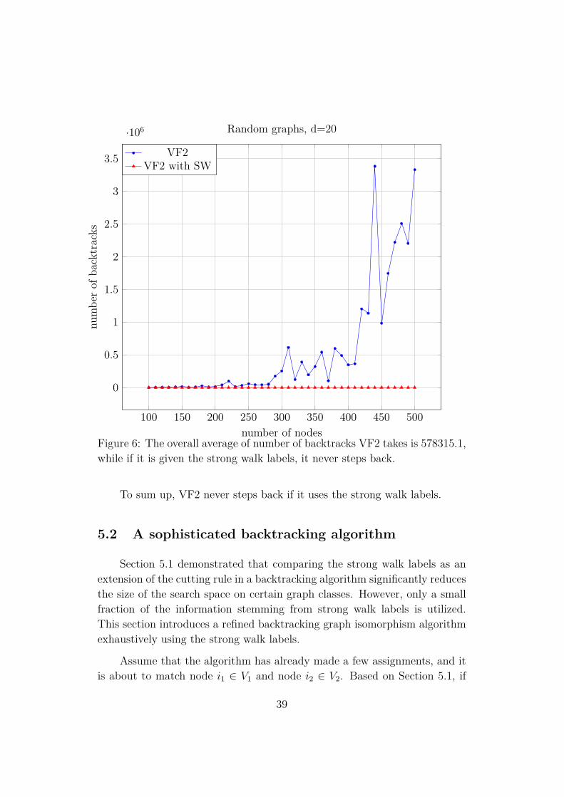
For a number d ∈ N and for each n = 100, 110, 120, ..500, generate15 d-regular graphs on n nodes, and randomly permute the nodes of eachgraph. For each of the 15 graphs, find an isomorphism between the mixedand the original graphs. The plots show the average number of backtrackswhile performing the 15 searches for each n. Figure 4, 5 and 6 show thed = 5, 10, 20 cases, respectively.
36

100 150 200 250 300 350 400 450 500
0
1
2
3
4
5
6
7
8·107
number of nodes
num
ber
ofba
cktr
acks
Random graphs, d=5
VF2VF2 with SW
Figure 4: The overall average of number of backtracks VF2 takes is 6497890.9,while if it is given the strong walk labels, it never steps back.
37

100 150 200 250 300 350 400 450 500
0
1
2
3
4
5
·106
number of nodes
num
ber
ofba
cktr
acks
Random graphs, d=10
VF2VF2 with SW
Figure 5: The overall average of number of backtracks VF2 takes is 774635.6,while if it is given the strong walk labels, it never steps back.
38
100 150 200 250 300 350 400 450 500
0
0.5
1
1.5
2
2.5
3
3.5
·106
number of nodes
num
ber
ofba
cktr
acks
Random graphs, d=20
VF2VF2 with SW
Figure 6: The overall average of number of backtracks VF2 takes is 578315.1,while if it is given the strong walk labels, it never steps back.
To sum up, VF2 never steps back if it uses the strong walk labels.
5.2 A sophisticated backtracking algorithm
Section 5.1 demonstrated that comparing the strong walk labels as anextension of the cutting rule in a backtracking algorithm significantly reducesthe size of the search space on certain graph classes. However, only a smallfraction of the information stemming from strong walk labels is utilized.This section introduces a refined backtracking graph isomorphism algorithmexhaustively using the strong walk labels.
Assume that the algorithm has already made a few assignments, and itis about to match node i1 ∈ V1 and node i2 ∈ V2. Based on Section 5.1, if
39

sG1(i1) 6 p= sG2(i2), then i1 and i2 can be never mapped together, therefore thecurrent branch can be pruned.
Observe that even if sG1(i1) p= sG2(i2), it might be the case that thereare nodes j1 ∈ V1 and j2 ∈ V2 s.t. node j1 ∈ V1 is already mapped to j2 ∈ V2
and the row of sG1(j1) corresponding to node i1 is different from the row ofsG2(j2) corresponding to i2. Clearly, the existence of such nodes j1 and j2
ensures that i1 can not be mapped to i2 in the current branch.
In other words, if the backtracking algorithm has already mapped certainnodes, then in this branch the permutation-equality of two node labels can bedefined in a more strict way. By definition, sG1(i1) p= sG2(i2) means that thereexist a permutation matrix P s.t. P sG1(i1) = sG2(i2). Now, the permutationmatrix can be prescribed to satisfy Pj2j1 = 1 for all (j1, j2) ∈ {(j1, j2) ∈ V1×V2
: j1 is mapped to j2 in the current branch}.
It is an open question whether there exists a graph pair for which thisalgorithm can be executed s.t. it steps back. Computational tests havebeen carried out on various graph classes including distance regular graphs,strongly regular graphs and other symmetric graph constructions, but thealgorithm has never stepped back. Investigating this question will be thebasis of a future research.
Note that if the algorithm never stepped back under depth O(logn), itwould solve the graph isomorphism problem in polynomial time. To provethat it does not solve the graph isomorphism problem, a graph sequenceshould be constructed s.t. the maximum number of backtracks the algorithmmight take tends to infinity asymptotically faster than logn.
The next section outlines an (induced) subgraph isomorphism algorithmalong the same idea.
5.3 The (induced) subgraph isomorphism problem
Observe that if G1 is searched in G2 and node i1 ∈ V1 can be mappedto node i2 ∈ V2, then there exists a permutation matrix P s.t. P`G1(i1)is element-wise not larger than `G2(i2). This immediately suggest a node-labeling for the (induced) subgraph isomorphism problem.
40
In addition, the sophisticated backtracking algorithm described in Sec-tion 5.2 is easy to adapt to this case.
Note that there is no straightforward way to use the strong walk la-bels instead of the walk labels. However, it is possible to support subgraphisomorphism algorithms similarly to the method developed for isomorphismalgorithms in Section 5.2. Based on preliminary computational tests, thismethods works well if the sizes (and the densities) of the two graphs arecomparable.
5.4 Graph fingerprints
Many practical graph matching algorithms are designed to solve thegraph isomorphism problem between two graphs as fast as possible, althoughin typical applications, say in biology, this task is rarely needed. Instead, agraph is searched in a graph database, which involves solving the graph iso-morphism problem many times. Supposing that each graph occurs only oncein the database, most of the graph pairs to be compared are not isomorphic.The idea is to define a graph-labeling s.t. for any two graphs their labels arethe same if the graphs are isomorphic, otherwise - apart from rare excep-tions - the labels are different. Such graph-labelings are called fingerprints.Graph fingerprints can be used to reduce the number of graph isomorphismproblems to be solved, since if the labels of the graphs are different, thenthey can not be isomorphic. In addition, if the fingerprints in a data baseare precomputed, one can filter out efficiently all the graphs having the samelabel as the graph to be searched does by using binary search tree or hashtable.
Sections 5.4.1 and 5.4.2 introduce two graph fingerprints using (strong)walk-labeling, and study their practical efficiency on graph databases con-taining biological, random and strongly regular graphs. Section 5.4.3 gener-alizes the graph fingerprint using strong walk labels.
The biological and the strongly regular graphs graphs were extractedfrom the Protein Data Bank [26] and from the homepage of Edward Spence[32], respectively.
41

5.4.1 Strong walk fingerprint
In the spirit of strong walk-labeling, matrix skG(i) corresponding to nodei is defined such that
skG(i)jl :=
H(δij + 2δjk), if l = 0H(skG(i)jl−1, {sG(i)i′l−1 : i′ ∈ ΓG(j)}#), otherwise
(16)
for all i, k, j ∈ [n] and for all l = 0..n. Note that skG(i) is a strangely initializedversion of sG(i).
Observe that the last column of skG(i) contains all information about theprevious ones, therefore it is sufficient to store the last element of each row.Let skG(i) denote the multiset of the values of the last column of skG(i).
To define the strong walk fingerprint, let
S(G) := H({H({H(skG(i)) : i ∈ [n]}#) : k ∈ [n]}#) (17)
By definition, the following claim holds.
Claim 5.4.1. If G1 and G2 are isomorphic, then S(G1) = S(G2).
To test this graph-labeling, a graph database was considered, and thefingerprint was generated to every graph. The graph database consists of10.000 biological graphs, 10.000 random 10-regular graphs on 1000 nodesand 43.753 strongly regular graphs.
It clearly shows the efficiency of fingerprint S that all generated S(G)labels were unique, i.e. two tested graphs are isomorphic if and only if theirlabel are the same. These experiments suggest that in general, two graphs areisomorphic if and only if their labels are the same. Note that this is unlikelyto hold, since, based on Section 3.2.1, this would imply a polynomial timegraph isomorphism algorithm.
It is easy to see that if an oracle can decide in polynomial time whethertwo graphs are isomorphic, then an isomorphism can also be constructed be-tween any to isomorphic graphs in polynomial time.
In the light of the following claim, the distinguishing power of strongwalk fingerprint is especially precious.
42

Claim 5.4.2. Any two strongly regular graphs with the same parameters arestrongly walk-isomorphic.
The relatively long yet straightforward proof is omitted.
To make sure of the correctness of the implementation, the followingtests were carried out. For each graph of the database, generate 10 isomor-phic graphs by permuting the nodes, and verify whether the 11 isomorphicinstances have the same graph fingerprint.
Finally, observe that the following claim follows from Theorem 4.2.1.
Claim 5.4.3. Two trees are isomorphic if and only if their strong walk fin-gerprints are equal.
Note that the computation time of S(G) labels can be reduced by con-sidering shorter walks only – possibly at the expense of the distinguishingpower. In addition, it is also easy to see that the length of considered walkscan be also chosen depending on the number of vertices (or edges).
5.4.2 Walk fingerprint
To define a weaker - but easier to compute - analogue of strong walkfingerprint, let the walk fingerprint be defined as follows.
L(G) := {`Gij: i, j ∈ [n], Gij = (V,E ∪ {(i, i), (j, j)})} (18)
The following claim is a direct consequence of the definition of the walkfingerprint.
Claim 5.4.4. If G1 and G2 are isomorphic, then L(G1) = L(G2).
These fingerprints were calculated for each graph in the database de-scribed in Section 5.4.1, as well. All of the biological and regular graphs hadunique fingerprints, but among the SRG’s there were 120 non-isomorphicgraph pairs having the same label.
43

5.4.3 Generalization of strong walk fingerprint
The equality of fingerprints given by S(G) seems to be equivalent to thegraph isomorphism – based on computational tests. Should it turn out tofail to distinguish two non-isomorphic graphs, a more general and strongergraph-labeling have been already developed. To describe this, first considerthe following notation.
sk1,..,kq
G (i)jl :=
H(δij +
q∑r=1
(r + 1)δjkr), if l = 0
H(skG(i)jl−1, {sG(i)i′l−1 : i′ ∈ ΓG(j)}#), otherwise(19)
where q ∈ N is a constant, j, k1, k2, .., kq ∈ [n] and l = 0..n are such thatk1 ≤ k2 ≤ .. ≤ kq.
Observe that the last column of sk1,..,kq
G (i) contains all information aboutthe previous ones, therefore it is sufficient to store the last element of eachrow. Let s
k1,..,kq
G (i) denote the multiset of the values of the last column ofsk1,..,kq
G (i).
Finally, the new, improved graph fingerprint is defined as follows.
Sq(G) := H({H({H(sk1,..,kq
G (i)) : i ∈ [n]}#) : k1 ≤ ... ≤ kq ∈ [n]}#) (20)
Claim 5.4.5. If G1 and G2 are isomorphic, then Sq(G1) = Sq(G2).
6 Conclusion and future work
This thesis introduced the concepts of walk-labeling and strong walk-labeling. After working out their theoretical background, various theoreticaland practical applications were presented. However, many interesting andimportant questions remain open. We conclude this work by presenting someof these questions and further ideas, which show the directions of the futurework, as well.
• Is walk-isomorphism equivalent to graph isomorphism on graphs havingsingle eigenvalues only?• Is walk-isomorphism equivalent to graph isomorphism on trees?
44

• Does walk-isomorphism distinguish graphs having different combinato-rial invariants, for instance k-connectivity?• Which of the results hold for the Laplacian eigenvalues as well?• There is no straightforward connection between quantum walks and the
strong labeling. Does one of the two approaches dominate the other?Is there a way to combine them?• The proposed sophisticated backtracking algorithm involves storing n2
node labels for each graph in the data base. Is there a way to reducethe necessary space?• Does there exist a graph sequence s.t. the proposed sophisticated back-
tracking algorithm might step back deeper that depth O(logn)?• To test the distinguishing power of the fingerprints on graphs of even
more graph classes.• Disprove (or prove) that the generalized strong walk fingerprint solves
the graph isomorphism problem.• Develop sufficient conditions under which the generalized strong walk
fingerprint solves the graph isomorphism problem. For example, onecould consider node labeled graphs s.t. the given labels determine a“fine” partition on the node set.• Is walk-isomorphism equivalent to graph isomorphism on cacti graphs?• Is walk-isomorphism equivalent to graph isomorphism on planer graphs?• Extend the methods to hypergraphs.• The graph isomorphism problem can be modeled as an IP by searching
a permutation matrix P s.t. PA1 = A2P . Using the proposed labels,one can strengthen the LP relaxation, in addition, cutting planes canbe generated during a Branch & Bound method. It would be interestingto characterize the graphs for which the relaxed polytope is integer (orto develop sufficient conditions).
7 Acknowledgement
The project was supported by the European Union, co-financed by theEuropean Social Fund (EFOP-3.6.3-VEKOP-16-2017-00002).
45

References
[1] QuantumBio Inc., http://www.quantumbioinc.com.
[2] V. Arvind, B. Das, J. Kobler, and S. Toda. Colored hypergraph iso-morphism is fixed parameter tractable. Algorithmica Volume 71, Pages120-138, January 2015.
[3] Laszlo Babai, D. Yu. Grigoryev, and David M. Mount. Isomorphismof graphs with bounded eigenvalue multiplicity. In Proceedings of theFourteenth Annual ACM Symposium on Theory of Computing, STOC’82, pages 310–324, New York, NY, USA, 1982. ACM.
[4] Norman Biggs. Algebraic Graph Theory. Cambridge University Press, 2edition, 1994.
[5] Vincenzo Bonnici, Rosalba Giugno, Alfredo Pulvirenti, Dennis Shasha,and Alfredo Ferro. A subgraph isomorphism algorithm and its appli-cation to biochemical data. BMC Bioinformatics. 14(Suppl 7): S13.,April 2013.
[6] Richard A. Brualdi and Dragos Cvetkovic. A Combinatorial Approachto Matrix Theory and Its Applications. CRC Press, 2009.
[7] Horst Bunke. Graph matching: Theoretical foundations, algorithms,and applications. In International Conference on Vision Interface,Pages 82-84,, May 2000.
[8] Charles J. Colbourn. On testing isomorphism of permutation graphs.Networks, Volume 11, Issue 1, Pages 13-21, March 1981.
[9] S. A. Cook. The complexity of theorem-proving procedures. Proc. 3rdACM Symposium on Theory of Computing, Pages 151-158, 1971.
[10] L. P. Cordella, P. Foggia, C. Sansone, and M. Vento. Performance eval-uation of the VF graph matching algorithm. Proc. of the 10th ICIAP,IEEE Computer Society Press, Pages 1172-1177, 1999.
[11] L. P. Cordella, P. Foggia, C. Sansone, and M. Vento. A (sub)graphisomorphism algorithm for matching large graphs. IEEE Transactionson Pattern Analysis and Machine Intelligence Volume 26 Issue 10, Page1367-1372, 2004.
46

[12] L. P. Cordella and M. Vento. Symbol recognition in documents: acollection of techniques? International Journal on Document Analysisand Recognition Volume 3, Issue 2, Pages 73-88,, December 2000.
[13] Balazs Dezso, Alpar Juttner, and Peter Kovacs. LEMON - an opensource C++ graph template library. Electronic Notes in TheoreticalComputer Science, 264(5):23 – 45, jul 2011. Proceedings of the SecondWorkshop on Generative Technologies (WGT) 2010.
[14] Brendan L Douglas and Jingbo B Wang. A classical approach to thegraph isomorphism problem using quantum walks. Journal of PhysicsA: Mathematical and Theoretical, 41(7):075303, 2008.
[15] A E. Brouwer and Edward Spence. Cospectral graphs on 12 vertices.Electr. J. Comb., 16, 06 2009.
[16] John King Gamble, Mark Friesen, Dong Zhou, Robert Joynt, and S. N.Coppersmith. Two-particle quantum walks applied to the graph isomor-phism problem. Physical Review A, 81:052313, May 2010.
[17] J. E. Hopcroft and J. K. Wong. Linear time algorithm for isomorphismof planar graphs. Proceeding STOC ’74 Proceedings of the sixth annualACM symposium on Theory of computing, Pages 172-184, April 1974.
[18] J. R. Ullmann. Bit-vector algorithms for binary constraint satisfac-tion and subgraph isomorphism. Journal of Experimental Algorithmics(JEA),Volume 15, Article No. 1.6, ACM New York, NY, USA, 2010.
[19] Alpar Juttner and Peter Madarasi. Vf2++—an improved subgraph iso-morphism algorithm. Discrete Applied Mathematics, 2018.
[20] Jianzhuang Liu and Yong Tsui Lee. A graph-based method for face iden-tification from a single 2D line drawing. IEEE Transactions on PatternAnalysis and Machine Intelligence - Graph Algorithms and ComputerVision archive Volume 23 Issue 10, Pages 1106-1119, October 2001.
[21] George S. Lue and Kellogg S. Booth. A linear time algorithm for decidinginterval graph isomorphism. Journal of the ACM (JACM), Volume 26,Issue 2, Pages 183-195, 1979, April 1979.
47

[22] Eugene M. Luks. Isomorphism of graphs of bounded valence can betested in polynomial time. Journal of Computer and System Sciences,Volume 25, Issue 1, Pages 42-65, August 1982.
[23] Peter Madarasi. Reszgraf megfeleltetesek keresese biologiai grafokban.OTDK, 2017.
[24] A Mahasinghe, J A Izaac, J B Wang, and J K Wijerathna. Phase-modified ctqw unable to distinguish strongly regular graphs efficiently.Journal of Physics A: Mathematical and Theoretical, 48(26):265301,2015.
[25] B. D. McKay. Practical graph isomorphism. Congressus Numerantium,Volume 30, Pages 45-87, 1981.
[26] Protein Data Bank. http://www.rcsb.org/pdb.
[27] D. Raviv, R. Kimmel, and A. M. Bruckstein. Graph isomorphisms andautomorphisms via spectral signatures. IEEE Transactions on PatternAnalysis and Machine Intelligence, 35(8):1985–1993, Aug 2013.
[28] Kenneth Rudinger, John King Gamble, Mark Wellons, Eric Bach, MarkFriesen, Robert Joynt, and Susan Coppersmith. Noninteracting multi-particle quantum random walks applied to the graph isomorphism prob-lem for strongly regular graphs. Phys. Rev. A, 86, 08 2012.
[29] Allen Schwenk. Almost all trees are cospectral. In New Directions in theTheory of Graphs, pages 275–307, New York, NY, USA, 1973. AcademicPress.
[30] Dennis Shasha, Jason T. L. Wang, and Rosalba Giugno. Algorithmicsand applications of tree and graph searching. In Proceedings of theTwenty-first ACM SIGMOD-SIGACT-SIGART Symposium on Princi-ples of Database Systems, PODS ’02, pages 39–52, New York, NY, USA,2002. ACM.
[31] Christine Solnon. Alldifferent-based filtering for subgraph isomorphism.Artificial Intelligence 174, Pages 850-86, 2010.
[32] Edward Spence. Strongly regular graphs on at most 64 vertices. http://www.maths.gla.ac.uk/˜es/srgraphs.php/.
48

[33] J. R. Ullmann. An algorithm for subgraph isomorphism. Journal of theACM (JACM), Volume 23 Issue 1, Pages 31-42, January 1976.
[34] Edwin R. van Dam and Willem H. Haemers. Which graphs are deter-mined by their spectrum? Linear Algebra and its Applications, 373(Sup-plement C):241 – 272, 2003. Combinatorial Matrix Theory Conference(Pohang, 2002).
[35] Mario Vento, Xiaoyi Jiang, and Pasquale Foggia. International conteston pattern search in biological databases, http://biograph2014.unisa.it.June 2015.
[36] Richard C. Wilson and Ping Zhu. A study of graph spectra for compar-ing graphs and trees. Pattern Recognition, 41(9):2833 – 2841, 2008.
49