the global rise of corporate saving - federal reserve … · the global rise of corporate ... we...
TRANSCRIPT

The Global Rise of Corporate Saving
Peter Chen University of Chicago
Loukas Karabarbounis University of Minnesota and Federal Reserve Bank of Minneapolis
Brent Neiman University of Chicago
Working Paper 736 Revised March 2017
Keywords: E21, E25, G32, G35 JEL classification: Corporate saving; Profits; Labor share; Cost of capital
The views expressed herein are those of the authors and not necessarily those of the Federal Reserve Bank of Minneapolis or the Federal Reserve System. __________________________________________________________________________________________
Federal Reserve Bank of Minneapolis • 90 Hennepin Avenue • Minneapolis, MN 55480-0291 https://www.minneapolisfed.org/research/
The Global Rise of Corporate Saving∗
Peter ChenUniversity of Chicago
Loukas KarabarbounisUniversity of Minnesota and FRB of Minneapolis
Brent NeimanUniversity of Chicago
March 2017
Abstract
The sectoral composition of global saving changed dramatically during the last three
decades. Whereas in the early 1980s most of global investment was funded by household
saving, nowadays nearly two-thirds of global investment is funded by corporate saving.
This shift in the sectoral composition of saving was not accompanied by changes in
the sectoral composition of investment, implying an improvement in the corporate net
lending position. We characterize the behavior of corporate saving using both national
income accounts and firm-level data and clarify its relationship with the global decline
in labor share, the accumulation of corporate cash stocks, and the greater propensity
for equity buybacks. We develop a general equilibrium model with product and capital
market imperfections to explore quantitatively the determination of the flow of funds
across sectors. Changes including declines in the real interest rate, the price of invest-
ment, and corporate income taxes generate increases in corporate profits and shifts in
the supply of sectoral saving that are of similar magnitude to those observed in the
data.
JEL-Codes: E21, E25, G32, G35.
Keywords: Corporate Saving, Profits, Labor Share, Cost of Capital.
∗This draft was prepared for the Carnegie-Rochester-NYU Conference on Public Policy in November 2016. We
thank Andrea Eisfeldt, Marvin Goodfriend, Burton Hollifield, and Eric Zwick for useful comments. We gratefully
acknowledge the support of the National Science Foundation. The accompanying Appendix and dataset are available
at the authors’ web pages. The views expressed herein are those of the authors and not necessarily those of the
Federal Reserve Bank of Minneapolis or the Federal Reserve System.

1 Introduction
Apple Inc., as of 2015 the world’s largest company by market capitalization, has generally in-
vested at a rate of roughly 20 to 30 percent of its gross value added. Apple’s flow of saving, by
contrast, has risen from levels of 20 to 30 percent of gross value added in the late 1980s and 1990s
to nearly 60 percent by 2013. Over this period, Apple’s profits grew precipitously and dividends
did not keep pace. Alongside this growth in Apple’s saving rate, the company accumulated a
massive stockpile of cash, has booked large amounts of operating income from subsidiaries all
over the world, and has recently repurchased its equity.
What might have caused the increase in Apple’s saving rate and how common is such an
increase? Is this rise unique to U.S. corporations, to technology companies, or to large multina-
tionals? How might it relate to changes in the cost of capital, profits, and corporate practices
on liquidity, repurchases, and transfer pricing? What are the macroeconomic implications?
We begin our analysis by constructing a dataset of sectoral saving and investment from
the national accounts of more than 60 countries. Consistent with previous studies such as
Poterba (1987), we measure corporate saving as undistributed corporate profits. We note that
corporate saving is a flow measure, distinct from the stock of savings accumulated through cash
or other financial assets, and equals physical investment plus net lending in the corporate sector.
Corporate saving together with government and household saving equal national saving.
We document a pervasive shift in the composition of saving away from the household sector
and toward the corporate sector. Global corporate saving has risen from below 10 percent of
global GDP around 1980 to nearly 15 percent in the 2010s. This increase took place in most
industries and in the large majority of countries, including all of the 10 largest economies. The
composition of investment spending across sectors was relatively stable over this period. The
corporate sector, therefore, transitioned from being a net borrower to being a net lender of funds
to the rest of the global economy.
What, in an accounting sense, caused the rise of corporate saving? Given that taxes and
interest payments on debt have remained essentially constant over time as shares of value added,
1
the rise of corporate saving mirrors the increase in corporate (accounting) profits and the decline
in the labor share documented previously for the global economy in Karabarbounis and Neiman
(2014). Corporate saving reflects the part of profits that is retained by the firm rather than paid
out as dividends. Since dividend payments have historically been “sticky” and did not increase
as much as profits, corporate saving grew secularly.1
We next study firm-level data and find, similarly to the national accounts data, that the
increase in corporate saving in the cross-section of firms reflects increases in firm profits and not
other forces such as changes in dividends, interest payments, or tax payments. Surprisingly, we
do not find evidence that trends in firm saving relate significantly to firm size and age. Increases
in corporate saving within industry, age, and size groups, rather than shifts in value added shares
between these groups, account for the majority of the global rise of corporate saving.
Further, we consider the possibility that multinationals, with their ability to shift production,
income, and tax liabilities across foreign business units, play a key role in the rise of corporate sav-
ing. The increase in corporate saving at the global level does not simply reflect the cross-country
shifting of profits and value added by multinationals because this reshuffling should cancel out
when aggregated across countries. Firms with significant income from foreign operations display
higher saving rates than firms without foreign income and this difference mainly reflects higher
shares of profits in value added rather than taxes or dividends. However, the share of firms with
significant foreign income in total value added is stable over time and, therefore, level differences
in saving rates across groups do not contribute to the overall rise of firm saving. These firms
exhibit larger increases in their saving rates but this difference is also accounted for by their
larger trend increase in profits rather than differential trends in dividend or tax payments.
The increase in corporate saving exceeded that in corporate investment, which implies that
the corporate sector improved its net lending position. Among other possibilities, increased net
lending can be associated with accumulation of cash, repayment of debt, or increasing equity
1The literature on the stickiness of dividends goes back to Lintner (1956). See Brav, Graham, Harvey, andMichaely (2005) and Fama and French (2001) for more recent evidence on sticky or declining dividends.
2

buybacks net of issuance.2 We demonstrate in the cross section of firms that the balance sheet
adjustment involved all three of these categories, though to an extent that varied over time.
Increases in net lending were more likely to be stockpiled as cash starting in the early 2000s and
were less likely to be used by firms to buy back their shares after the financial crisis.
To quantify how observed changes in parameters affect the cost of capital and corporate sav-
ing, profits, financial policies, and investment, we study a workhorse dynamic general equilibrium
model with heterogeneous firms and product and capital market imperfections. Our modeling
is inspired by a literature at the intersection of corporate finance and macroeconomics, which
departs from the Modigliani and Miller (1958) and Miller and Modigliani (1961) irrelevance
theorems by incorporating collateral constraints, equity flotation costs, and differential taxes on
capital gains, interest, and dividends.3 These imperfections imply that firms face a higher cost of
capital than what would arise in an undistorted economy and often prefer to finance operations
from internal saving.
We parameterize the model to represent the global economy in the early years of our sample.
We compare this initial equilibrium to a new one that emerges when we subject the model to
changes in several parameter values that we estimate from the data. The model generates a
decline in the cost of capital of roughly 3 percentage points and an increase in the corporate
saving rate of equal magnitude to that documented in the data. Quantitatively, we find that
important drivers of this change are the global declines in the real interest rate, the price of
investment goods, and corporate income taxes and the increase in markups. The mechanism
is that, with an elasticity of substitution above one in production, the decline in the cost of
capital and the increase in markups both lead to a decline in the labor share and an increase in
corporate profits. Given the stability of dividends relative to GDP, this increase in profits leads
to an increase in corporate saving. Further, firms have tax incentives to buy back more shares
as saving increases and this lead to an improvement in the corporate net lending position.
2As highlighted by Bates, Kahle, and Stulz (2009) who emphasize precautionary motives and Foley, Hartzell,Titman, and Twite (2007) who emphasize repatriation taxes, cash holdings have risen markedly relative to assets.
3Important contributions in this literature include Gomes (2001), Hennessy and Whited (2005), Riddick andWhited (2009), Gourio and Miao (2010), and Jermann and Quadrini (2012).
3

2 Corporate Saving in the National Accounts
We now describe the construction of our national income accounts dataset and review the national
income accounting framework which relates corporate saving to the corporate labor share, profits,
and dividends. We then document the widespread rise of corporate saving relative to GDP,
corporate gross value added, and total saving over the past several decades.
2.1 National Accounts Data
We obtain annual data at the national and sector levels by combining information downloaded
online or obtained digitally from the United Nations (UN) and Organization for Economic Co-
operation and Development (OECD). Over time and across countries there are some differences
in methodologies, but these data generally conform to System of National Accounts (SNA)
standards. We refer the reader to Lequiller and Blades (2006) for detailed descriptions of how
national accounts are constructed and harmonized to meet these standards.
We exclude countries that do not have raw data on corporate saving or gross fixed capital
formation. The resulting dataset contains sector-level information on the income structure of 66
countries for various years between 1960 and 2013. The OECD data cover 30 member countries
but offer more disaggregated items than the UN counterpart. All our analyses start on or after
1980, the earliest year for which we have at least eight countries (Finland, France, Germany,
Italy, Japan, Netherlands, Norway, and the United States). The United Kingdom enters the
sample in 1989 and China enters in 1992. By 2007, the sample consists of over 60 countries that
account for more than 85 percent of global GDP.
2.2 National Accounts Structure and Identities
National accounts data include sector accounts that divide the economy into the corporate sector,
the government sector, and the household and non-profit sector. For most economies, the cor-
porate sector can be further disaggregated into financial and non-financial corporations and the
4
household sector can be distinguished from the non-profit sector.4 National accounts data also
include industry accounts that divide activity according to the International Standard Industrial
Classification, Rev. 4 (SIC).
A set of accounting identities that hold in the aggregate as well as at the sector or industry
level serve as the backbone for the national accounts. In these accounts, the value of final
production (i.e. production net of intermediate goods) is called gross value added (GVA). When
aggregated to the economy level, GVA equals GDP less net taxes on products.5 GVA is detailed
in the generation of income account and equals the sum of income paid to capital, labor, and
taxes:
GVA = Gross Operating Surplus (GOS) + Compensation to Labor
+ Net Taxes on Production. (1)
GOS captures the income available to corporations and other producing entities after paying for
labor services and after subtracting taxes (and adding subsidies) associated with production.
The distribution of income account splits GOS into gross saving, dividends, and other pay-
ments to capital such as taxes on profits, interest payments, reinvested foreign earnings, and
other transfers:
GOS = Gross Saving (GS) + Net Dividends︸ ︷︷ ︸Accounting Profits
+ Taxes on Profits + Interest
− Reinvested Earnings on Foreign Direct Investment + Other Transfers. (2)
Net dividends equal dividends paid less dividends received from subsidiaries or partially-owned
entities. Other transfers include social contributions and rental payments on land. In our
4For countries with missing information on corporate sector gross value added, we impute their values by multi-plying country GDP by the global corporate gross value added to GDP ratio. To impute the missing corporate laborshare, we multiply the labor share found in the total economy by the global ratio of corporate labor share to totallabor share. After imputing the corporate gross value added and labor compensation, we impute missing productiontaxes by subtracting gross operating surplus and labor compensation from gross value added. The Appendix furtherdiscusses details such as when we use the UN or OECD data, how we treat outliers, and some country-specificadjustments.
5The treatment of taxes net of subsidies on products (that includes items such as excise taxes, state and local salestaxes, and taxes and duties on imports) in most countries differs from that in the U.S. NIPA tables. For instance,in many countries some subset of the taxes are not allocated to sectors. This means that while they contribute tooverall GDP, they do not contribute to the gross value added of any sector.
5
analyses, we define (accounting) profits as the sum of gross saving and net dividends.
The capital account connects the flow of saving to the flow of investment as follows:
GS = Net Lending + Gross Fixed Capital Formation + Changes in Inventories
+ Changes in Other Non-Financial Produced Assets. (3)
The net lending position is defined as the excess of gross saving over investment spending.
2.3 Sectoral Saving Trends
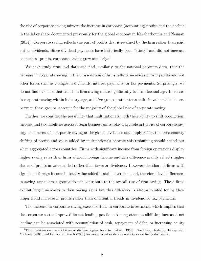
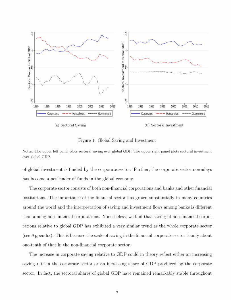
Figure 1(a) plots the evolution of gross saving in each of the three sectors relative to global GDP
since 1980. Government saving exhibits cyclical fluctuations but it has not exhibited secular
trends relative to GDP. Households and corporations, however, exhibit striking trends. Saving
by corporations has increased by nearly 5 percentage points relative to GDP whereas saving by
households has decreased by nearly 6 percentage points.6
We generate these lines by pooling all countries with saving data for all three sectors and
regressing the ratios of sector saving to GDP on time fixed effects. We weight the regressions by
GDP, translated at market exchange rates, and we control for changes in the country composition
of our unbalanced panel by absorbing country fixed effects. To benchmark the level of the lines,
we pool all available countries in our data in 2013 and calculate the appropriate global value.
We then use the estimated time fixed effects to extrapolate that level backwards. All subsequent
plots at the global level from the national accounts data are constructed equivalently.
For the world as a whole, gross saving must equal gross investment, but this need not be true
at the sector level. Indeed, as Figure 1(b) shows, the sectoral composition of global investment
has remained largely stable over time, in contrast to the sectoral composition of global saving.
Whereas in 1980 the household sector funded most of global investment, in modern times most
6Most of our data adhere to SNA standards, which consider as corporations any entities that (i) aim to generateprofit for their owners, (ii) are legally recognized as being separate entities from their owners, who have only a limitedliability, and (iii) were created to engage in market production. Economic activities undertaken by households orunincorporated enterprises that are not separate legal entities with a full set of accounts to distinguish its business-related assets and liabilities from the personal assets and liabilities of its owners are considered part of the householdsector. Implicit rental payments earned by homeowners constitute an important piece of the household sector.
6
-.0
50
.05
.1.1
5S
ecto
ral S
avin
g t
o G
lob
al G
DP
1980 1985 1990 1995 2000 2005 2010 2015
Corporates Households Government
(a) Sectoral Saving-.
05
0.0
5.1
.15
Se
cto
ral In
ve
stm
en
t to
Glo
ba
l G
DP
1980 1985 1990 1995 2000 2005 2010 2015
Corporates Households Government
(b) Sectoral Investment
Figure 1: Global Saving and Investment
Notes: The upper left panel plots sectoral saving over global GDP. The upper right panel plots sectoral investment
over global GDP.
of global investment is funded by the corporate sector. Further, the corporate sector nowadays
has become a net lender of funds in the global economy.
The corporate sector consists of both non-financial corporations and banks and other financial
institutions. The importance of the financial sector has grown substantially in many countries
around the world and the interpretation of saving and investment flows among banks is different
than among non-financial corporations. Nonetheless, we find that saving of non-financial corpo-
rations relative to global GDP has exhibited a very similar trend as the whole corporate sector
(see Appendix). This is because the scale of saving in the financial corporate sector is only about
one-tenth of that in the non-financial corporate sector.
The increase in corporate saving relative to GDP could in theory reflect either an increasing
saving rate in the corporate sector or an increasing share of GDP produced by the corporate
sector. In fact, the sectoral shares of global GDP have remained remarkably stable throughout
7
.1.2
.3.4
.5.6
Sec
tora
l Sav
ing
to S
ecto
ral G
VA
1980 1985 1990 1995 2000 2005 2010 2015
Corporates Households
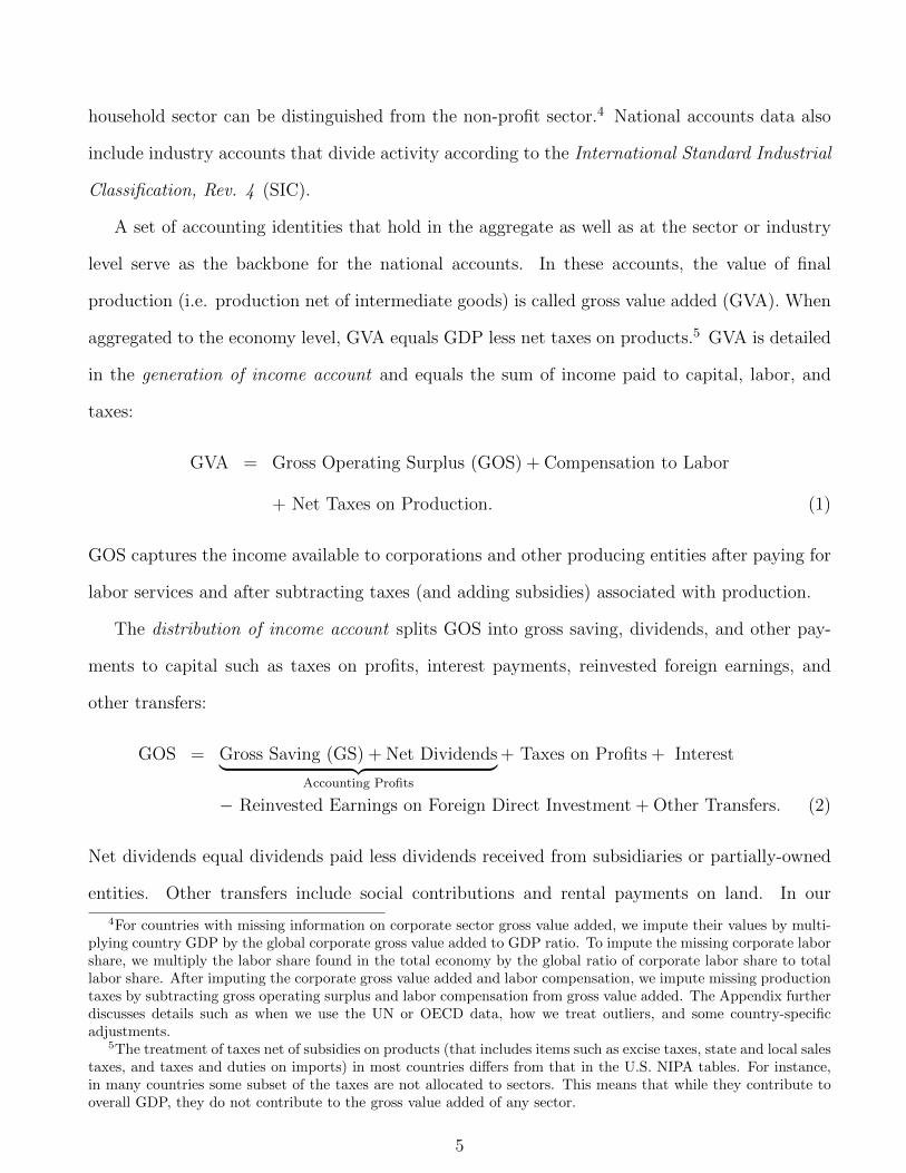
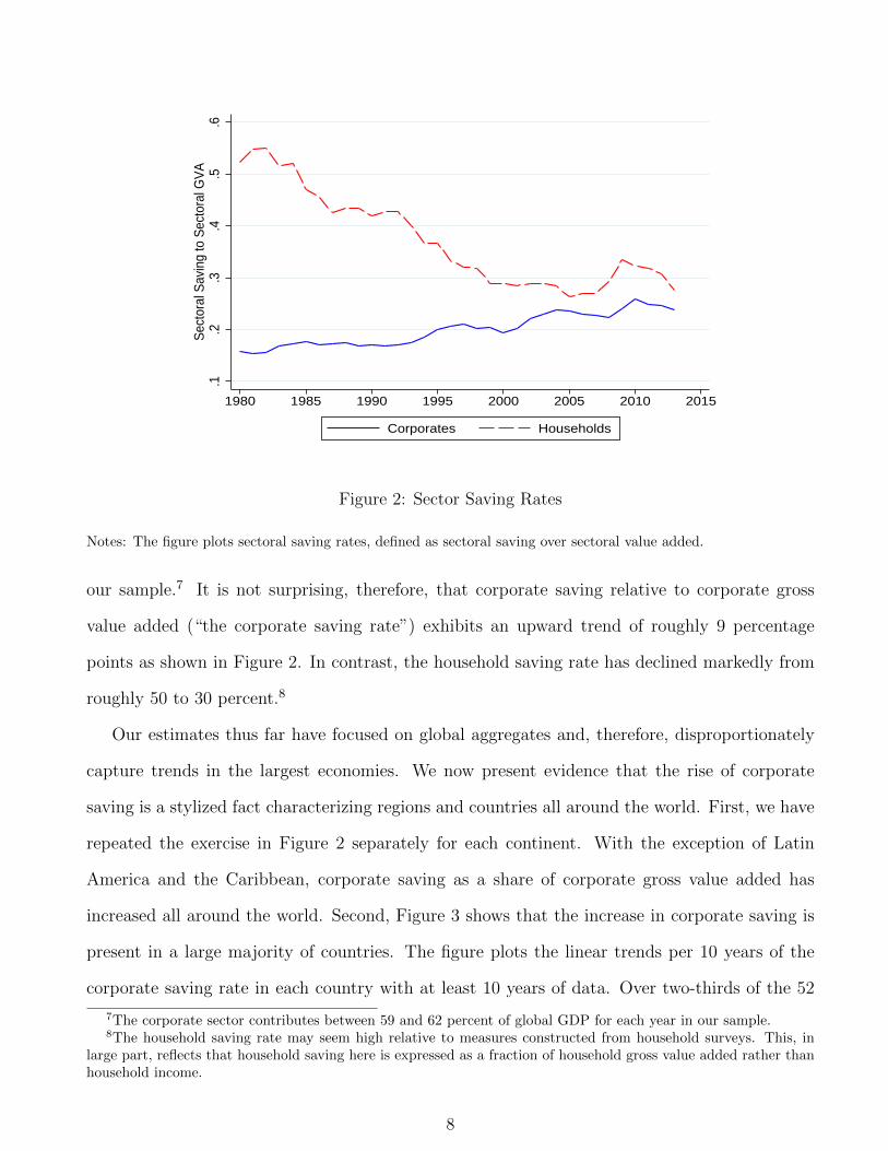
Figure 2: Sector Saving Rates
Notes: The figure plots sectoral saving rates, defined as sectoral saving over sectoral value added.
our sample.7 It is not surprising, therefore, that corporate saving relative to corporate gross
value added (“the corporate saving rate”) exhibits an upward trend of roughly 9 percentage
points as shown in Figure 2. In contrast, the household saving rate has declined markedly from
roughly 50 to 30 percent.8
Our estimates thus far have focused on global aggregates and, therefore, disproportionately
capture trends in the largest economies. We now present evidence that the rise of corporate
saving is a stylized fact characterizing regions and countries all around the world. First, we have
repeated the exercise in Figure 2 separately for each continent. With the exception of Latin
America and the Caribbean, corporate saving as a share of corporate gross value added has
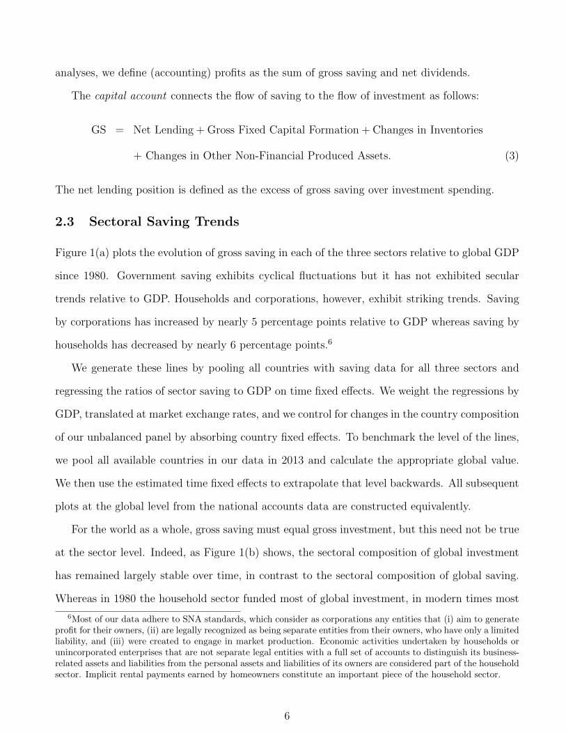
increased all around the world. Second, Figure 3 shows that the increase in corporate saving is
present in a large majority of countries. The figure plots the linear trends per 10 years of the
corporate saving rate in each country with at least 10 years of data. Over two-thirds of the 52
7The corporate sector contributes between 59 and 62 percent of global GDP for each year in our sample.8The household saving rate may seem high relative to measures constructed from household surveys. This, in
large part, reflects that household saving here is expressed as a fraction of household gross value added rather thanhousehold income.
8

Bra
zil
U
K
U
SG
erm
any
Fra
nce
Can
ada
Ita
ly
Jap
an
Chi
na
Kor
ea
-50
510
Per
cent
age
Poi
nt In
crea
se p
er 1
0 Y
ears
Figure 3: Trends in Corporate Saving Rates
Notes: The figure plots trends per 10 years in corporate saving rates by country.
countries included, and all 10 of the world’s largest economies (the shaded bars in the figure),
have seen increases in their corporate saving rate.9
By construction, as the corporate saving rate increases, the share contributed by other com-
ponents of gross value added must decrease. Substituting the definition of gross operating surplus
from equation (2) into equation (1), and applying it to the corporate sector, we write a decom-
position of corporate gross value added:
Corporate GVA = Corporate Compensation to Labor + Corporate Taxes
+ Corporate Payments to Capital + Corporate Gross Saving, (4)
where we define taxes as the sum of net taxes on production and taxes on profits and define
payments to capital as the sum of dividends, interest, reinvested earnings on foreign direct
investment, and other transfers. Equation (4) shows that an increase in the saving share of
9Our global results are consistent with other studies of various subsamples. Bacchetta and Benhima (2015)document the increase in corporate saving for fast-growing emerging economies. Bayoumi, Tong, and Wei (2012)use listed firms to document the upward trend in China and selected other countries. Armenter and Hnatkovska(2014) use balanced sheet data and show the improvement in the net lending position of U.S. firms.
9
0.2
.4.6
Share
of C
orp
ora
te G
VA
1980 1985 1990 1995 2000 2005 2010 2015
Compensation to Labor Payments to CapitalTaxes Gross Saving
(a) GVA Components0
.1.2
.3S
hare
of C
orp
ora
te G
VA
1990 1995 2000 2005 2010 2015
Interest DividendsTransfers Saving
(b) Saving, Dividends, and Interest
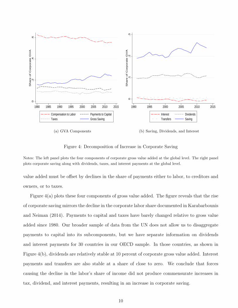
Figure 4: Decomposition of Increase in Corporate Saving
Notes: The left panel plots the four components of corporate gross value added at the global level. The right panel
plots corporate saving along with dividends, taxes, and interest payments at the global level.
value added must be offset by declines in the share of payments either to labor, to creditors and
owners, or to taxes.
Figure 4(a) plots these four components of gross value added. The figure reveals that the rise
of corporate saving mirrors the decline in the corporate labor share documented in Karabarbounis
and Neiman (2014). Payments to capital and taxes have barely changed relative to gross value
added since 1980. Our broader sample of data from the UN does not allow us to disaggregate
payments to capital into its subcomponents, but we have separate information on dividends
and interest payments for 30 countries in our OECD sample. In those countries, as shown in
Figure 4(b), dividends are relatively stable at 10 percent of corporate gross value added. Interest
payments and transfers are also stable at a share of close to zero. We conclude that forces
causing the decline in the labor’s share of income did not produce commensurate increases in
tax, dividend, and interest payments, resulting in an increase in corporate saving.
10

3 Corporate Saving at the Firm Level
In this section, we use firm-level data to study the cross-sectional patterns in the rise of corporate
saving rates. An important finding of our analysis is that much of this rise is accounted for
by increasing saving rates within groups of firms and industries and does not simply reflect
shifting market shares between groups with differing saving rate levels. Additionally, we discuss
how multinational activity may have impacted the trend in corporate saving and we study the
relationship between net lending and cash holdings, equity buybacks, and repayment of debt in
the cross section of firms.
3.1 Firm-Level Data
We obtain consolidated financial statement data of publicly listed firms from Compustat Global
and Compustat North America.10 We treat the financial statements at the end of each company’s
fiscal year as if it reflected their activities during the corresponding calendar year. We convert
all local currency values to U.S. dollars using annual average exchange rates.
There are three main differences between our national accounts dataset and our firm-level
dataset. First, as with most analyses of firm-level financing decisions that focus on non-financial
corporations such as Fama and French (2001) and DeAngelo, DeAngelo, and Skinner (2004),
we exclude financial firms (SIC codes 6000-6999). We also exclude other unclassified firms (SIC
codes greater than or equal to 9000) as well as firms for which we cannot calculate a gross saving
rate for at least 10 years. Second, economic activities in the firm-level data are classified by the
country of headquarters as opposed to the country of operation. For example, the production
of a U.S. subsidiary operating in France would be captured in the consolidated statement of
the U.S. parent and the subsidiary itself would not have any record included in our firm-level
dataset. This differs from the treatment in the national accounts, where production, profits, and
investment are all classified by the country of operation, as opposed to headquarters. A third
10The word “consolidated” refers to the consolidation between parent and subsidiaries. By law, parent companiesmust submit consolidated statements. Non-consolidated statements, on the other hand, are typically not mandatory.We exclude non-consolidated statements to avoid double counting of firm activities.
11
difference with the national accounts is that the firm-level data includes only publicly listed
firms.
We now describe key variables used in our firm-level analysis, many of which are unavailable
in Compustat in raw format. First, gross value added is defined as gross output less interme-
diate consumption, but intermediate consumption is not available. To impute it, we start with
operating expenses, which we calculate as the sum of the costs of goods sold (COGS) and selling,
general, and administrative (SG&A) expenses, both of which are available as raw data:
Operating Expensesf,c,i,t = COGSf,c,i,t + SG&Af,c,i,t, (5)
where f , c, i, and t index firms, countries, industries, and years, respectively. To obtain inter-
mediate consumption, we would then need to subtract depreciation, research and development
(R&D), staff compensation, and production taxes from operating expenses:11
Intermediate Consumptionf,c,i,t = Operating Expensesf,c,i,t −Depreciationf,c,i,t − R&Df,c,i,t
− Staff Compensationf,c,i,t − Production Taxesf,c,i,t︸ ︷︷ ︸Not Available in Compustat
. (6)
The difficulty is that, while we have firm-level data on operating expenses, depreciation, and
R&D, data on staff compensation and production taxes – the last two terms of equation (6) –
are generally not reported in Compustat.
Our approach is to impute intermediate consumption at the firm level using information on
a firm’s operating expenses and the relationship between operating expenses and intermediate
consumption found in industry-level data from national accounts. We begin by approximating
the share of intermediate consumption in operating expenses net of depreciation and R&D in
country c, industry i, and year t, πc,i,t, using the industry-level information in the national
11The national accounts definition of intermediate consumption includes the products and non-labor servicesconsumed in the production process, such as produced inputs, rental payments for structures and equipment, pur-chases of office supplies, usage of water and electricity, advertisement costs, overhead costs, market research cost,and administrative costs. Intermediate consumption excludes depreciation, research and development expenses,compensation to labor, and taxes levied during the production process.
12
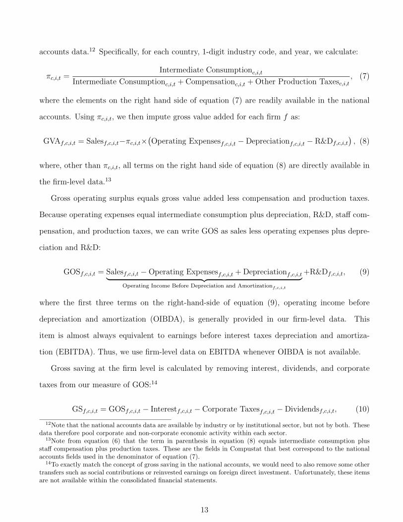
accounts data.12 Specifically, for each country, 1-digit industry code, and year, we calculate:
πc,i,t =Intermediate Consumptionc,i,t
Intermediate Consumptionc,i,t + Compensationc,i,t + Other Production Taxesc,i,t, (7)
where the elements on the right hand side of equation (7) are readily available in the national
accounts. Using πc,i,t, we then impute gross value added for each firm f as:
GVAf,c,i,t = Salesf,c,i,t−πc,i,t×(Operating Expensesf,c,i,t −Depreciationf,c,i,t − R&Df,c,i,t
), (8)
where, other than πc,i,t, all terms on the right hand side of equation (8) are directly available in
the firm-level data.13
Gross operating surplus equals gross value added less compensation and production taxes.
Because operating expenses equal intermediate consumption plus depreciation, R&D, staff com-
pensation, and production taxes, we can write GOS as sales less operating expenses plus depre-
ciation and R&D:
GOSf,c,i,t = Salesf,c,i,t −Operating Expensesf,c,i,t + Depreciationf,c,i,t︸ ︷︷ ︸Operating Income Before Depreciation and Amortizationf,c,i,t
+R&Df,c,i,t, (9)
where the first three terms on the right-hand-side of equation (9), operating income before
depreciation and amortization (OIBDA), is generally provided in our firm-level data. This
item is almost always equivalent to earnings before interest taxes depreciation and amortiza-
tion (EBITDA). Thus, we use firm-level data on EBITDA whenever OIBDA is not available.
Gross saving at the firm level is calculated by removing interest, dividends, and corporate
taxes from our measure of GOS:14
GSf,c,i,t = GOSf,c,i,t − Interestf,c,i,t − Corporate Taxesf,c,i,t −Dividendsf,c,i,t, (10)
12Note that the national accounts data are available by industry or by institutional sector, but not by both. Thesedata therefore pool corporate and non-corporate economic activity within each sector.
13Note from equation (6) that the term in parenthesis in equation (8) equals intermediate consumption plusstaff compensation plus production taxes. These are the fields in Compustat that best correspond to the nationalaccounts fields used in the denominator of equation (7).
14To exactly match the concept of gross saving in the national accounts, we would need to also remove some othertransfers such as social contributions or reinvested earnings on foreign direct investment. Unfortunately, these itemsare not available within the consolidated financial statements.
13

where interest, corporate taxes, and dividends are items available in our firm-level data. Finally,
we measure gross fixed capital formation as the acquisition less sale and disposals of property,
plant, and equipment, plus R&D expenditure.15
Table 1 provides an overview of the resulting firm-level dataset. We rank countries by their
aggregated gross value added recorded in the dataset and present statistics for the largest 25
countries. We reiterate that these firm-level data classify activity across countries differently
from the national accounts and include only publicly listed firms. Direct comparisons with GDP,
therefore, are not particularly informative. Nonetheless, aggregated across all countries in 2013,
firms in our sample contributed roughly 15.5 trillion U.S. dollars of gross value added, which
represents roughly 60 percent of the global non-financial corporate gross value added found in
the national accounts. Despite the differences between what is measured and reported in our
macro and micro data, the global (non-financial) saving rate aggregated up from the firm-level
data tracks well the saving rate we measured from the national accounts (see Appendix).
3.2 Corporate Saving in the Cross Section of Industries
Is the rise of corporate saving primarily concentrated in specific industries or is it broad-based?
Is the rise caused by growth in the saving rate within industries or does it reflect the changing
size of industries with differing levels of saving rates? To answer these questions, we begin by
aggregating saving, net lending, and value added from the firm-level data up to the country and
industry level. For each industry, we then regress the saving rate and the net lending rate on a
linear time trend, absorbing country fixed effects. We weight these regressions with countries’
gross value added in that industry to obtain a representative global trend for each industry.
We present our results in Table 2. The first column presents the average share of an indus-
try’s value added in global value added. Adding up all shares (other than the manufacturing
subsectors) yields 100 percent of global value added.16 The third column presents the estimated
15We ignore changes in the value of inventories in our firm-level measure of investment. While plausibly importantover short horizons, this is unlikely to impact our results which focus on long-term trends.
16The 44 percent of global value added accounted for by manufacturing in 2013 in our firm-level data exceedsestimates of manufacturing’s share of global GDP, which are closer to 17 percent according to the World Bank. Someof this difference reflects the fact that in the firm-level data we have value added contributed only by non-financial
14

Table 1: Summary of Firm-Level Data
CountryGross Value Added in 2013
Number of Firms Earliest Year($Billions, USD)
United States 4772.5 3232 1989
Japan 2843.2 2385 1989
China 994.6 1279 1995
United Kingdom 853.7 978 1989
France 808.6 447 1989
Germany 716.3 428 1994
Korea 360.2 360 1995
Russia 328.9 73 1996
India 279.3 1870 1995
Brazil 266.2 202 1992
Netherlands 260.4 109 1991
Switzerland 255.7 163 1991
Taiwan 232.5 1112 1994
Australia 218.5 359 1991
Italy 174.3 149 1994
Canada 169.6 414 1989
Hong Kong 166.8 503 1992
Spain 164.9 56 1994
Sweden 155.4 204 1994
Mexico 138.4 80 1994
South Africa 114.7 162 1992
Thailand 94.4 334 1993
Norway 92.3 91 1993
Singapore 87.4 368 1995
Chile 79.1 118 1994
Notes: The table presents summary statistics of the firm-level data.
15

Table 2: Industry Trends
Industry Value Added Share Saving Rate Net Lending Rate
(p.p. per 10 years)
Agriculture and Mining 3.77 3.20 -1.00(0.16) (0.50)
Construction 2.82 0.41 0.70(0.10) (0.17)
Information and Communications 6.79 -3.40 1.80(0.19) (0.44)
Total Manufacturing 44.43 1.95 1.49(0.04) (0.11)
Manufacturing Subsectors:
Chemical, Petro, and Coal 14.31 1.01 0.24(0.08) (0.21)
Electronics and Electrical 7.43 2.79 4.53(0.05) (0.14)
Transportation Equipment 7.06 1.94 0.60(0.12) (0.25)
Rubber, Plastic, Glass, Metal 6.67 0.77 0.30(0.09) (0.18)
Other Manufacturing 8.96 2.12 1.78(0.03) (0.08)
Services 7.23 2.43 4.44(0.07) (0.08)
Transportation 3.79 -1.83 -1.65(0.08) (0.14)
Utilities 3.95 -6.06 -9.14(0.11) (0.35)
Wholesale/Retail Trade 27.21 0.60 0.96(0.02) (0.03)
Notes: The table presents trends (in percentage points per 10 years) in saving and net lending rates by industry.
16

trend in the saving rate, expressed in percentage point changes per 10 years, along with its
standard error. Most industries experienced statistically significant increases in their corporate
saving rate. The exceptions, Information and Communications, Transportation, and Utilities,
only represent a total of 14.5 percent of value added in our data. The fourth column shows that
a clear majority of industries also experienced improvements in their net lending positions.
We use a standard within-between decomposition to quantify the extent to which the changes
in the corporate saving rate reflect changes within or between industries. Denoting groups of
firms by i = 1, ..., I, we decompose changes in the aggregate saving rate into these components
as follows:
∆
(GSt
GVAt
)=
1
2
∑i
(ωi,t + ωi,t−1) ∆
(GSi,t
GVAi,t
)︸ ︷︷ ︸
Within-Group Component
+1
2
∑i
(GSi,t
GVAi,t+
GSi,t−1
GVAi,t−1
)∆ωi,t︸ ︷︷ ︸
Between-Group Component
, (11)
where ∆xt = xt−xt−1 and ωi,t denotes the share of group i in total gross value added in period t.
Here, we use the industries in Table 2 to define the groups, so that the first component in equation
(11) reflects changes within industries over time holding constant their share of economic activity
and the second component reflects changes between industries as their share of economic activity
changes over time.
Applying this decomposition to the change in our full sample from 1989 to 2013, we find
that 7.6 of the 8.7 percentage points increase in the global corporate saving rate is accounted
for by the within-industry component. For the United States, we actually find that the between
component is negative. Taken together with our result that the increase in corporate saving is
observed in most countries, we conclude that the increase is pervasive across types of economic
activity and does not reflect long-term structural changes at the industry or global level.
3.3 Accounting for the Rise of Saving Using Firm-Level Data
In Section 2.3 we used national income accounts data to argue that the trend in corporate saving
reflects the decline in the labor share and the increase in corporate profits because dividends,
corporations and so we exclude the contribution to GDP from sectors like finance, government, and households(including implied rental income). An additional difference may reflect the greater propensity for manufacturers tobe publicly listed and, therefore, included in our firm-level dataset.
17
−10
−5
05
10T
rend
in S
avin
g to
Gro
ss V
alue
Add
ed
−10 −5 0 5 10Trend in Gross Operating Surplus to Gross Value Added
(a) Gross Saving
−10
−5
05
10T
rend
in D
ivid
ends
to G
ross
Val
ue A
dded
−10 −5 0 5 10Trend in Gross Operating Surplus to Gross Value Added
(b) Dividends
−10
−5
05
10T
rend
in In
tere
st to
Gro
ss V
alue
Add
ed
−10 −5 0 5 10Trend in Gross Operating Surplus to Gross Value Added
(c) Interest
−10
−5
05
10T
rend
in T
axes
to G
ross
Val
ue A
dded
−10 −5 0 5 10Trend in Gross Operating Surplus to Gross Value Added
(d) Taxes
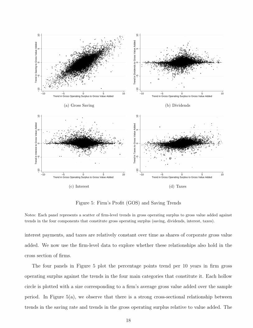
Figure 5: Firm’s Profit (GOS) and Saving Trends
Notes: Each panel represents a scatter of firm-level trends in gross operating surplus to gross value added against
trends in the four components that constitute gross operating surplus (saving, dividends, interest, taxes).
interest payments, and taxes are relatively constant over time as shares of corporate gross value
added. We now use the firm-level data to explore whether these relationships also hold in the
cross section of firms.
The four panels in Figure 5 plot the percentage points trend per 10 years in firm gross
operating surplus against the trends in the four main categories that constitute it. Each hollow
circle is plotted with a size corresponding to a firm’s average gross value added over the sample
period. In Figure 5(a), we observe that there is a strong cross-sectional relationship between
trends in the saving rate and trends in the gross operating surplus relative to value added. The
18

other three panels show that trends in dividend, interest, and tax payments are weakly correlated
with trends in the gross operating surplus.
To quantify these relationships we regress each variable plotted in the y-axis on the trend
in gross operating surplus relative to gross value added, controlling for country and industry
fixed effects.17 Weighting with gross value added, the slope coefficient for Figure 5(a) is 0.74,
suggesting that every dollar increase in gross operating surplus in the cross section of firms is
associated with an increase of 74 cents in corporate gross saving. From the other three categories,
only the regression with taxes produces a meaningfully positive coefficient (it equals 0.16). When
we do not weight our regressions with gross value added, we generally obtain similar results.
3.4 Corporate Saving in the Cross Section of Firms
Is growth in firm saving most prevalent among large or small firms? Is it driven by young and
rapidly growing firms or by older firms? In this section we assess the extent to which the rise
of corporate saving reflects changes within particular types of firms or changes across firms with
different characteristics and levels of saving.
The rise of corporate saving could reflect compositional changes over time if the average
propensity to save varies with firm characteristics. The upper panels of Figure 6 present scatter-
plots of the average saving rate against log firm size (measured as the average share of the firm in
aggregate sales) and firm age (measured as the firm’s mean year in the sample minus the year of
its IPO). The regression coefficient (weighted by gross value added) corresponding to Figure 6(a)
is 0.0006 with a standard error of 0.003, controlling for country and industry fixed effects.18 This
estimate implies that firms with twice the value of another firm’s sales (i.e. an increase of 0.69
log points) have roughly a 0.04 percentage point higher saving rate. The regression coefficient
(weighted by gross value added) corresponding to Figure 6(b) is -0.0003 with a standard error of
0.0002, controlling for country and industry fixed effects. This means that firms that are 10 years
older have a 0.3 percentage point lower saving rate. We conclude that the average propensity to
17In these and later regressions of firm-level data, we winsorize all variables at the top and bottom 1 percent.18We cluster the standard errors at the country level in all regressions in that use averages or trends of firm-level
variables.
19

-.5
0.5
1S
avin
g to
Gro
ss V
alue
Add
ed
-18 -15 -12 -9 -6 -3log Sales
(a) Saving Rate Level and Log Sales
-.5
0.5
1S
avin
g to
Gro
ss V
alue
Add
ed
0 10 20 30 40 50 60 70Age
(b) Saving Rate Level and Firm Age
-10
-50
510
Tre
nd in
Sav
ing
to G
ross
Val
ue A
dded
-18 -15 -12 -9 -6 -3log Sales
(c) Saving Rate Trend and Log Sales
-10
-50
510
Tre
nd in
Sav
ing
to G
ross
Val
ue A
dded
0 10 20 30 40 50 60 70Age
(d) Saving Rate Trend and Firm Age
Figure 6: Saving Rate and Firm Characteristics
Notes: The upper panels plot saving rates against firm log average sales (left panel) and firm age (right panel). The
lower panels plot trends in saving rates against firm log average sales (left panel) and firm age (right panel). Each
firm’s sales are normalized by aggregate sales in that year to account for inflation over the years in our dataset.
Each firm’s age is calculated as their last year in the dataset minus their year of incorporation.
save does not vary significantly with firm size and age.
We use the decomposition in equation (11) to quantify the extent to which changes in the
corporate saving rate reflect changes within or between groups of firms. In Table 3 we present
decompositions in which groups i = 1, ..., I are defined either by the quartile of a firm in the
age distribution or the quartile of a firm in the size distribution or the union of the two.19 In
19In this decomposition we focus only on firms that have information on age. We group firms into size and agegroups depending on the quartile that their size or age belongs to in each year.
20

Table 3: Within-Between Decompositions of Changes in Saving Rate
Saving to Gross Value Added (p.p.)
Beginning to End (1989-2013) Cumulative Annual Changes
Within Between Within Between
(1) (2) (3) (4)
Size 12.11 0.29 12.10 0.29
Age 10.17 2.23 7.61 4.79
Size and Age 10.39 2.01 7.38 5.01
Notes: The table presents results from the within-between decomposition presented in equation (11) for groups of
firms i defined by quartiles of age, quartiles of size, or the union of them.
columns 1 and 2, we present the decomposition of the cumulative change from the beginning to
the end of the sample. Essentially all of the increase in the corporate saving rate is due to the
within-group component, irrespective of whether groups are defined by the quartiles of size or
age or both. In columns 3 and 4, we perform the decomposition annually and then cumulate the
changes from the beginning to the end of the sample. We find that the change in the corporate
saving rate is entirely because of the within-size component. While some of the increase in the
corporate saving rate is due to the between age and between age and size components, again the
majority of the increase is accounted for by increases in the within components.
Given the salience of the within components to the growth in corporate saving rates, we
conclude this section by asking if this growth is heterogeneous in age or size at the firm level.
The lower panels of Figure 6 present scatterplots that relate the trend in saving over value added
for each firm per 10 years to log firm size and age. As we see in these scatters, there is no clear
pattern that relates the trend in saving to either size or age.20
20The regression coefficient (weighted by gross value added) corresponding to Figure 6(c) is -0.107 with a standarderror of 0.137, controlling for country and industry fixed effects. This estimate implies that firms with twice thevalue of another firm’s sales (i.e. an increase of 0.69 log points) have roughly a 0.07 percentage point lower trendin their saving rate per 10 years. The equivalent regression coefficient corresponding to Figure 6(d) is -0.03 with astandard error of 0.01, implying that firms that are 10 years older have a 0.03 percentage point lower trend in their
21
Taken together, the results in Sections 3.2 to 3.4 suggest that the growth in corporate saving
is not primarily driven by basic characteristics such as firm size or age and is not specific to a
small number of industries. Much like our conclusion from analysis of the national accounts,
these firm-level data paint a picture of a global and pervasive phenomenon. It is unlikely to
reflect structural changes such as the decline in manufacturing, idiosyncratic changes in the
market power of particular firms or industries, or changes in the corporate financial practices of
particular firms or countries.21
3.5 The Impact of Multinational Production
The operations of multinationals across countries have grown in importance in recent decades.
Since a company’s gross saving is associated with its headquarters country, moving production to
foreign subsidiaries might increase the corporate saving rate in the headquarters country because
it preserves the numerator (gross saving) while lowering the denominator (gross value added).
If shifting of production or profits reduces the gross value added associated with each dollar
of saving in the headquarters country, then the opposite increase of equal magnitude would be
observed in the country where production occurred or where profits were realized. To the extent
that our country coverage is sufficiently broad, the effects of reshuffling profits and production
across countries on corporate saving rates should cancel out in our data at the global level.22
The Appendix presents a stylized example that illustrates this logic.
Multinationals might also impact trends in corporate saving given they might have a different
propensity to pay taxes and issue dividends. Levin and McCain (2013) and Clausing (2011)
detail, for example, how multinationals use transfer pricing and various accounting rules to realize
saving rate per 10 years. The Appendix additionally presents versions of Figure 6 plotting aggregated bins of firms,rather than individual firms, which largely corroborate these conclusions.
21This finding is interesting in light of previous research documenting that the pattern of disappearing dividendsreflects a shift in the composition of firms toward smaller and less profitable firms with higher growth prospects(Fama and French, 2001).
22Keightley (2013) emphasizes the disproportionate recording of U.S. profits in Bermuda, Ireland, Luxembourg,the Netherlands, and Switzerland. It is possible that our dataset – which has less than 10 years of data on Bermuda,Luxembourg, and Switzerland – disproportionately captures the headquarters countries, in which case the reshufflingof profits would not necessarily cancel out at the global level. But even among Ireland and the Netherlands, forwhich we have long time series, we observe large increases in their corporate saving rates.
22
as much of their global profits as possible in low tax jurisdictions.23 Further, multinationals may
pay less dividends to avoid paying the resulting tax on repatriated foreign earnings.
To study these issues, we first need to distinguish multinationals from other firms in our
dataset. While multinational status is not directly observable in our data, our analysis dis-
tinguishes between firms that have less than one percent of their income earned outside their
headquarters country (roughly 50 percent of the firms in our data) and those earning greater
than one percent of their income abroad. Firms with a higher fraction of foreign income have
the greatest ability and interest in shifting income across countries to avoid taxes. We perform
our analysis only in the U.S. data as we cannot construct the foreign income variable for other
countries.
Firms in the group with more than one percent of their income earned abroad display a
saving rate that is roughly 4 to 6 percentage points higher than firms with less than one percent
of their income earned abroad. Surprisingly, this difference mainly reflects a higher share of gross
operating surplus in value added – likely reflecting lower labor shares – rather than differences
in taxes or dividends.24 Because the value added share of each group of firms is essentially
constant since the beginning of the sample, shifts of economic activity between these groups do
not contribute to changes in the aggregate firm saving rate.
Firms with more than one percent of their income earned abroad also experienced a larger
trend increase in their saving rates. This difference, however, resulted primarily from faster
growth in their gross operating surpluses. We do not find that firms with greater foreign income
had significantly lower growth in taxes or dividends relative to gross value added or gross oper-
ating surplus. This finding is consistent with our previous conclusion that the rise of firm saving
reflects the decline in the labor share and the rise of corporate profits.
23Guvenen, Mataloni, Rassier, and Ruhl (2016) emphasize the possibility that foreign subsidiaries “underpay” forinputs provided by U.S. parents. This phenomenon may be most prevalent when the input is an intangible assetsuch as a patent.
24These results are presented in the Appendix and control for firm size, firm age, and industry fixed effects. Wenote that the saving rates of the two groups of firms are different at conventional significance levels only when wedo not weight the regressions.
23
3.6 How Was the Increase in Corporate Net Lending Used?
An increase in the flow of corporate saving can be used for a combination of expenditures in phys-
ical investment, accumulation of cash and other financial assets, repayment of debt obligations,
or increases in equity buybacks net of issuances. Our analysis documents that the difference
between corporate saving and investment increased over time. In this section, we provide evi-
dence that links trends in the net lending position of firms to trends in their net buybacks, debt
repayment, and cash accumulation.
We first clarify that national accounts treat equity buybacks as if they were negative is-
suances. Therefore, the value of equity buybacks net of issuances is part of corporate saving
and net lending. Such a treatment is reasonable in our view because it implies no changes in
corporate saving were a firm to simultaneously issue and then repurchase the same value of
shares. Aggregating net buybacks with dividends would be economically meaningful if the two
were perfect substitutes.25 In the Appendix we show that subtracting the value of net equity
buybacks from corporate saving does not affect significantly the evolution of the global corporate
saving rate shown in Figure 2. This result is consistent with Gruber and Kamin (2016) who also
document a small trend in net buybacks as a share of GDP among OECD economies.
Table 4 reports results from regressions in the firm-level data that link trends in the net
lending position of firms to trends in their net buybacks, debt repayment, and cash accumula-
tion.26 All regressions include country and industry fixed effects. The first two columns consider
regressions where the left-hand-side variable is the trend in the ratio of net buybacks to gross
value added and the right-hand-side variable is the trend in net lending relative to value added.
For the full sample between 1989 and 2013, presented in row A, we find that firms experiencing a
25However, capital gains from repurchases are often taxed differentially from dividends and tax authorities mayput limits on buybacks. Additionally, equity issuance is costly and its cost is likely to vary cyclically (Eisfeldt andMuir, 2016).
26Net buybacks are defined as value of equity buybacks net of equity issuance (corresponding to variables“PRSTKC” - “SSTK”). Net repayment of debt is defined as repayment of long term debt minus issuance of longterm debt and changes in current debt (corresponding to “DLTR” - “DLTIS” - “DLCCH”). Cash accumulation isdefined as cash assets and short-term investments (corresponding to “CHE”). Data limitations preclude us from afull decomposition of net lending, so various other balance sheet items including the accumulation of other financialassets are subsumed in a residual category.
24

Table 4: Uses Net Lending: Buybacks, Debt Repayment, and Cash Accumulation
Net Buybacks Net Repayment Change inof Equity of Debt Cash Holdings
(1) (2) (3) (4) (5) (6)
(A) Full Sample 0.267 0.277 0.397 0.343 0.322 0.057(0.064) (0.071) (0.051) (0.048) (0.142) (0.054)
(B) 1989 to 2000 0.174 0.326 0.516 0.346 0.053 -0.075(0.098) (0.075) (0.149) (0.067) (0.074) (0.028)
(C) 2001 to 2013 0.130 0.129 0.346 0.337 0.312 0.050(0.029) (0.026) (0.067) (0.051) (0.127) (0.049)
(D) 1989 to 2006 0.275 0.292 0.481 0.393 0.172 -0.042(0.090) (0.076) (0.050) (0.050) (0.063) (0.058)
(E) 2007 to 2013 0.098 0.074 0.446 0.435 0.218 0.050(0.028) (0.018) (0.082) (0.051) (0.053) (0.031)
GVA Weighted Yes No Yes No Yes No
Notes: Columns 1 and 2 present estimated coefficients and their standard errors from firm-level regressions of the
trend in the net buyback to value added ratio on the trend in the net lending to value added ratio. Columns 3 and 4
present estimated coefficients and their standard errors from firm-level regressions of the trend in the net repayment
of debt to value added ratio on the trend in the net lending to value added ratio. Columns 5 and 6 present estimated
coefficients and their standard errors from firm-level regressions of the trend in cash standardized by mean value
added on the trend in net lending standardized by mean value added. All standard errors are clustered by country.
one percentage point higher trend increase in their net lending rate increased their net buybacks
by 0.267 (when we weight) or 0.277 (when we do not weight) additional percentage point relative
to value added.
Columns 3 and 4 show that firms experiencing a one percentage point higher trend increase
in their net lending rate increased their net repayment of debt by 0.397 (when we weight) or
0.343 (when we do not weight) additional percentage point relative to value added. Columns 5
and 6 report results from regressions of the trend in cash on saving and net lending. Since cash
25

is a stock variable, these regressions consider trends in the levels of cash and net lending but
with all variables divided by the firm’s average gross value added to create a scale-independent
measure. We find that roughly 32 cents (when we weight) or 6 cents (when we do not weight)
of each dollar of trend increase in net lending was accumulated in cash.27
Rows B through E of Table 4 document how these relationships between net lending and
buybacks, repayment of debt, and accumulation of cash evolve during subperiods of our sample.
Rows B and C repeat these regressions in the early (1989 to 2000) and later (2001 to 2013)
years of the sample and rows D and E repeat the regressions before (1989 to 2006) and after the
financial crisis (2007 to 2013). We find that the propensity of firms to increase their buybacks in
response to net lending fell markedly during and after the financial crisis relative to the decades
prior. Net lending only led to the accumulation of cash starting in the 2000s. Discussion in the
policy literature of the large corporate cash stockpiles often emphasize increases in uncertainty,
especially after the global recession of 2008-2009. These results indeed suggest there was a change
in corporate preference for liquidity, though they suggest the change predates the recent crisis.28
4 Corporate Saving and Capital Market Imperfections
In this section we develop a general equilibrium model with capital market imperfections that
allows us to quantify how changes in parameters affect the cost of capital, the flow of funds
between corporations and households, and other key macroeconomic aggregates. We calibrate
our model to represent the global economy around 1980. Given the pervasiveness of the rise
of corporate saving across countries, industries, and types of firms, we subject the model to
parameter changes that represent common global trends, such as changes in the real interest rate,
27Bates, Kahle, and Stulz (2009) and Foley, Hartzell, Titman, and Twite (2007) have emphasized the accumulationof cash on corporate balance sheets. Falato, Kadyrzhanova, and Sim (2013) argue that the secular trend in U.S.corporate cash holdings reflects the rising importance of intangible capital as an input of production. If intangiblecapital is more difficult to pledge as collateral, firms reduce the cost of financing externally their intangible capitalaccumulation by increasing their cash holdings.
28Warsh (2006) emphasizes the growing significance of foreign operations of U.S. multinationals and uncertaintyeven before the 2008-2009 recession. Carney (2012) stresses the elevated levels of uncertainty following the 2008-2009recession. Within the macroeconomics literature, the decision to increase corporate cash holdings in response touncertainty shocks has been recently examined by Alfaro, Bloom, and Lin (2016).
26
price of investment goods, markups, and other aspects of firms’ cost of capital. We then assess
the extent to which the model reproduces the evolution of corporate saving, profits, financial
policies, and investment as seen in the world.
4.1 Description of the Model
We consider an infinite horizon model with periods t = 0, 1, 2, ... and no aggregate uncertainty.
Model periods denote years. The economy is populated by identical households, a government,
and heterogeneous firms i = 1, ..., N that supply differentiated varieties of a final good and face
idiosyncratic productivity shocks.
Growth. Our quantitative results focus on comparisons across different balanced growth paths
of the model economy. Along any given balanced growth path, the economy is growing at a
constant exogenous rate g given by the growth rate of the population. Denoting initial labor by
L̃0, the population in period t > 0 is L̃t = (1+g)tL̃0. In what follows, we write the model directly
in terms of stationary variables that are detrended by their respective growth rates. Thus, if
x̃t is a variable growing at a rate gx = {0, g} along the balanced growth path, the detrended
variable xt is defined as xt = x̃t/(1 + gx)t.
Households. Households choose consumption Ct, bonds Bt+1, and shares sit+1 to maximize
the objective function∑∞
t=0 βt log (Ct). Households supply labor inelastically. Normalizing the
price of consumption to one in each period, the budget constraint is given by:
Ct +∑i
vitsit+1 + (1 + g)Bt+1 = wtL+ (1 + rt)Bt +∑i
((1− τdt )dit − eit + vit
)sit + T ht , (12)
where vit denotes the (ex-dividend) price of a share of firm i, wt denotes the wage per unit of
L, rt denotes the (risk-free) real interest rate, τdt is the tax rate on dividend income, dit denotes
dividend distributions from firms to households, eit denotes the value of net equity flows from the
household to firms, and T ht denotes lump-sum transfers from the government to the household.
Note that eit denotes the value of net equity issuance which equals the difference between
the value of equity issuance and the value of share repurchases. The value of net equity issuance
eit enters with a negative sign in the right hand side of the budget constraint because issuance
27
dilutes equity and reduces capital gains. For simplicity, capital gains inclusive of the impact of
dilution and repurchases, vit+1− vit− eit, are not taxed and, therefore, τdt should be understood
as a function of the gap between taxes on dividends and capital gains.
Final good. Producers of the final good are perfectly competitive and produce aggregate output
Yt by combining intermediate goods yit according to a CES function Yt =(∑
i yεε−1
it
) εε−1
, where
ε > 1 is the elasticity of substitution between varieties. Denoting by pit the price of variety i and
by Pt the price of output, the profit maximization problem of the final goods producer yields the
demand functions yit = (pit/Pt)−ε Yt. Intermediate goods are monopolistically competitive and,
therefore, there are economic profits in equilibrium equal to a fraction sπ = 1/ε of total income
in the economy.
Final output is used for consumption, investment, and resource costs related to the adjustment
of capital and the issuance of equity. Producers of the consumption good transform one unit of
final output Yt into one unit of consumption Ct. Our normalization of the price of consumption
to one implies Pt =(∑
i p1−εit
) 11−ε = 1. Producers of the investment good transform one unit of
final output Yt into 1/ξt units of investment Xt, where ξt denotes the price of investment relative
to consumption. Resource costs RCt equal the sum of resource costs related to the adjustment
of the capital stock and the issuance of equity and are denominated in terms of final output.
The goods market clearing condition is given by Yt = Ct + ξtXt + RCt.
Corporations producing intermediate goods. Corporations are owned by households. Our
analysis focuses on balanced growth paths with no aggregate uncertainty and, therefore, firms
apply the household’s stochastic discount factor in a balanced growth path to value streams of
payoffs. Following Auerbach (1979), Poterba and Summers (1985), and Gourio and Miao (2010,
2011), each firm chooses dividends dit, equity eit, debt bit+1, investment xit, labor `it, and the
price of its variety pit to maximize discounted net payments to shareholders:
max{dit,eit,bit+1,xit,`it,pit}∞t=0
E0
∞∑t=0
βt{
(1− τdt )dit − eit}, (13)
where (1− τdt )dit−eit denotes after-tax dividends and the value of equity repurchases less equity
28

injections. While for concreteness we call negative values of eit equity repurchases, we think of
eit < 0 more broadly as capturing all pre-dividend distributions or transactions that affect the
net lending position of firms and are perceived by firms as creating value for shareholders.29
Whenever τdt > 0, reductions in eit are the preferred means of transferring resources to
shareholders. We sidestep the issue of why firms prefer to pay dividends rather than create
capital gains to shareholders by assuming that, for institutional reasons, firm dividends are
equal to a target level of dividends that depends on revenues and the value of fixed assets:
dit = κ (pityit)κr (ξtkit)
κk . (14)
In equation (14), pityit denotes firm’s revenues and ξtkit denotes the value of fixed capital. We
choose to model dividends as a function of variables that are sufficient statistics for a firm’s state
vector (productivity and capital). Because productivity is not directly observed in the firm-level
data, we use revenues as a proxy and treat the data and the model similar in that respect. In
our quantitative application, the elasticities κr and κk are disciplined from firm-level data on
dividends, revenues, and fixed assets.
Following Gomes (2001) and Hennessy and Whited (2005), equity financing is costly because
of asymmetric information or transaction costs. Specifically, for each unit of new equity raised
in period t, only (1 − λ)eit units actually augment the firm’s funds, where λ ∈ [0, 1]. Flotation
costs are given by ECit = λeitI (eit ≥ 0), where It is an indicator taking the value of one when
firms issue equity. Firms can buy back their shares (eit < 0) without costs.
Firms operate a CES production function:
yit = exp (Ait)(αk
σ−1σ
it + (1− α)`σ−1σ
it
) σσ−1
, (15)
where σ denotes the elasticity of substitution between capital and labor and α denotes a distribu-
tion parameter. In the limiting case of σ → 1, the production function becomes Cobb-Douglas,
29As we discussed in Section 3.6, the increase in net lending only partially reflected an increase in equity repurchasesnet of issuance. In a stationary state of our model, bond positions do not change and the net lending position ofthe corporate sector depends only on eit. We therefore interpret changes in eit broadly to include other unmodeledfactors that lead shareholders to value changes in the firm’s net lending position.
29
yit = exp (Ait) kαit`
1−αit . Productivity Ait is the only exogenous stochastic process that firms face.
It follows an AR(1) process in logs:
Ait = − σ2A
2(1 + ρA)+ ρAAit−1 + σAuit with uit ∼ N(0, 1), (16)
where ρA denotes the persistence of the productivity process and σA denotes the standard devi-
ation of productivity shocks.
Firms issue debt that, as in Kiyotaki and Moore (1997), is limited by a collateral constraint:
bit+1 ≤ θξt+1kit+1, (17)
where θ ≥ 0 denotes the leverage parameter. Interest payments on debt are tax deductible and,
therefore, firms prefer to issue debt rather than equity. For this reason, we assume that the
collateral constraint always binds (see Appendix for more details).
Firms own the capital stock and augment it by purchasing investment goods. The law of
motion for capital is given by (1 + g)kit+1 = (1− δ)kit + xit. Firms face convex adjustment costs
CCit = ψ (kit+1 − kit)2 / (2kit) to change their capital stock.
Defining operating profits as πit = pityit − wt`it, the flow of funds constraint of the firm is
given by:30
dit+(1 + τxt ) ξtxit+(1+rt)bit+RCit = (1−τ ct )πit+τct (δξtkit + rtbit)+τ ft +(1+g)bit+1+eit, (18)
where τxt is the tax rate on investment spending, RCit = CCit + ECit, τct is the corporate tax
rate, and τ ft is a lump sum transfer from the government. Depreciation and interest payments,
δξtkit + rtbit, are deducted from firm earnings in calculating taxes. Firm lump sum transfers are
τ fit = χYt/N , so that they always represent a constant fraction χ of total output. The variable
T ft =∑
i τfit = χYt denotes total firm lump sum transfers.
Equilibrium. An equilibrium for this economy is defined as a sequence of prices and quantities
such that households and firms maximize their values, the government budget constraint holds,
30The difference between the term “operating profits” used here and “accounting profits” used in the empiricalsections is that our notion of operating profits, equivalent to earnings before interest and taxes in the firm-leveldata, does not remove interest and taxes.
30
and goods, labor, and capital markets clear (see Appendix for a more detailed description). We
define a stationary equilibrium as an equilibrium in which all (detrended) aggregate variables
are constant and the distribution of firms across states (kit, Ait) is stationary over time.
Saving Flows. Total domestic saving equals investment spending, St = Yt − Ct − RCt = ξtXt,
and can be decomposed into household and firm saving, St = Sht + Sft . Firm saving equals:
Sft = (1− τ ct ) (Yt − wtL) + τ ct (δξtKt + rtBt) + T ft − τxt ξtXt − RCt − rtBt −Dt + gBt+1. (19)
Using the flow of funds of firms, we show that the three uses of corporate saving are reductions
in debt, reductions in equity issuance, and investment spending:
Sft = Bt −Bt+1 − Et + ξtXt. (20)
Parameterization. Our strategy is to choose parameters in order to match statistics in the
early years of our sample, which we treat as being generated from an initial balanced growth
path of our model. To parameterize the model, we use a variety of aggregate statistics from our
national accounts dataset and other sources and moments estimated from our firm-level data
that inform heterogeneity in firm technologies and in frictions influencing corporate financial
policy. We present details of the parameterization in the Appendix. Here we summarize our
choice of the most important parameters for our results.31
The elasticity of substitution between capital and labor is set equal to σ = 1.25, the value
estimated in Karabarbounis and Neiman (2014) from cross-country covariation in trends in the
labor share and the relative price of investment goods. We set the growth rate to g = 0.023,
consistent with data from the World Bank, and set the discount factor β so that the model
generates a real interest rate equal to r = (1 + g)/β − 1 = 0.043. This value equals the world
real interest rate estimated by King and Low (2014) in the first year of their sample (1985) using
data on ten-year inflation-protected government bonds. Tax rates are obtained from the OECD
tax databases.
31Parameters values not discussed in the text are: α = 0.292, δ = 0.074, ξ = 1, sπ = 0.05, θ = 1.7, λ = 0.028,τd = 0.17, τ c = 0.48, τx = 0.117, χ = 0.037, κ = 0.17, ψ = 5.5, ρA = 0.8, and σA = 0.48.
31

Table 5: Model Results
Start of Sample Sf
YwLY
DY
IY
Sf−IY
R
1. Data 0.162 0.612 0.101 0.215 -0.053
2. Model 0.162 0.612 0.101 0.215 -0.053 0.153
End of Sample (∆) Sf
YwLY
DY
IY
Sf−IY
R
3. Data 0.085 -0.054 0.005 -0.006 0.091
4. Model 0.081 -0.054 -0.001 0.019 0.062 -0.031
Counterfactuals (∆) Sf
YwLY
DY
IY
Sf−IY
R
5. No ξ 0.057 -0.029 -0.003 -0.005 0.062 0.005
6. No τ c 0.048 -0.045 0.001 0.006 0.042 -0.028
7. No r -0.015 -0.026 -0.005 -0.051 0.036 0.007
8. No sπ 0.055 -0.026 -0.002 0.001 0.054 -0.027
Notes: The variables Sf , wL, D, and I denote corporate saving, compensation to labor, dividends, and the invest-
ment expenditure and are expressed as a share of corporate value added Y . For all variables the data entries in
the beginning of the sample (row 1) refer to world averages between 1980-1984 with the exception of dividends that
refer to world averages between 1990-1994. The data entries in the end of the sample (row 3) refer to world averages
between 2009-2013. The variable R denotes the equilibrium cost of capital defined in equation (22).
The elasticities κr and κk in the dividend policy function are estimated from the following
regression applied to our firm-level dataset:
log (Dividends)ict = bi+ bc+ bt+κr log (Sales)ict+κk log (Book Value of Capital)ict+uict, (21)
where bi, bc, and bt denote firm, country, and time fixed effects. We obtain values of κr = 0.63
and κk = 0.05 with standard errors (clustered at the firm level) of around 0.01 in both cases. As
shown below, these firm-level estimates imply a significant rigidity of dividends at the aggregate
level.
32

4.2 Quantifying the Increase in Corporate Saving in the Model
Table 5 summarizes our results. Row 1 lists values for the corporate saving rate Sf/Y , the labor
share sL = wL/Y , the dividend to output ratio D/Y , the investment rate I/Y , and the corporate
net lending position (Sf − I)/Y in the early years of our sample (generally 1980-1984). Row
2 lists the corresponding values generated by the initial balanced growth path of our economy.
By construction, our model is calibrated to match exactly the data along these statistics in the
early years of our sample. Along with these statistics, the table presents the model’s equilibrium
aggregate cost of capital defined by:
R =(1− sL − sπ)Y
K. (22)
The initial cost of capital equals 0.153 and reflects a combination of technological parameters,
interest rates, taxes, and financial frictions. Defining the “frictionless” cost of capital as ξ(r+δ) =
0.117, capital market imperfections in our model lead to an (aggregate) capital wedge of 3.6
percentage points (or 30 percent).
Row 3 summarizes changes in aggregate variables for the global economy between the initial
(generally 1980-1984) and final years of our sample (2009-2013). As discussed in Section 2.3, the
global corporate saving rate increased by 8.5 percentage points and the labor share declined by
5.4 percentage points. Dividends and investment spending remained roughly constant relative
to gross value added.
Our goal is to compare aggregates measured at the end of our data with those generated along
a new balanced growth path that differs from the initial one due to the following changes. We set
ξ = 0.8 to capture the 20 percent decline in the relative price of investment goods over the past
three decades, documented in Karabarbounis and Neiman (2014). We calculate a decline in the
corporate income tax rate τ c from 0.48 to 0.25 and in the world interest rate r from 0.043 to 0.009.
We estimate an increase in the depreciation rate δ from 0.074 to 0.093. We use the updated
series from McDaniel (2007) to estimate an increase in investment tax rates τx of roughly 26
percent from 0.117 to 0.148. We set the growth rate to zero percent to mimic the slowdown of
33

world economic activity in the aftermath of the Great Recession. Finally, we calculate increased
values for sπ (from 0.050 to 0.062) and χ (from 0.037 to 0.059) so that the model generates the
observed decline in the labor share and stability of taxes as a share of corporate value added
documented previously in the data.
Row 4 of Table 5 contains the main result of our analysis. The model generates a roughly
3 percentage points decline in the cost of capital. Along with this decline, the corporate saving
rate increases and the labor share decreases by magnitudes that are close to the changes observed
in the data.
To understand the mechanism driving this behavior, we use equation (19) to derive the
corporate saving rate in a stationary environment (dropping time subscripts denotes detrended
variables that are constant in a balanced growth path):
Sf
Y= 1− wL
Y︸︷︷︸Labor Share
− D
Y︸︷︷︸Dividends
−[τ c(
1− wL+ δξK
Y
)+τxξX + RC− T f + ((1− τ c)r − g)B
Y
]︸ ︷︷ ︸
Taxes and Other Payments to Capital
.
(23)
The decomposition in equation (23) shows that the corporate saving rate decreases with the
labor share, with the dividend rate, with net taxes, and with other payments to capital.
We begin our analysis by deriving an equation for the labor share of income for a represen-
tative firm with revenues Y that faces a cost of capital R, markups µ, and technology exp(A):
wL
Y=
(1
µ
)(1− ασ
(exp(A)
µR
)σ−1). (24)
Equation (24) shows that, with an elasticity of substitution in production σ > 1, the decline
in the cost of capital induces firms to substitute away from labor and toward capital to such a
degree that the share of income accruing to labor declines. Given the stability of payments to
taxes, the decline in the labor share implies an increase in the share of profits. This leads to an
increase in the corporate saving rate as long as dividends relative to value added do not increase
by the same amount.
Indeed, as shown in the third column of Row 4, the stability of dividends relative to gross
value added in our model is quantitatively consistent with the behavior of dividends in the data.
34

From the dividend policy function in equation (14) we see that the dividend to output ratio for
a representative firm with revenues Y is given by:
D
Y= κ
(ξK
Y
)κk ( 1
Y
)1−κr−κk. (25)
Our estimates of κk = 0.05 and κr = 0.63 from our firm-level data imply that the dividend
to output ratio is increasing in the capital-output ratio and decreasing in output. Following
the decline in the cost of capital, both the capital-output ratio and output increase, leading
to a relatively stable D/Y . As discussed in Section 3.6, the decision by firms how to allocate
profits among dividends, financial assets, and net buybacks is critical to the behavior of corporate
saving. This specification of the dividend process, estimated from cross-sectional variation in
our firm-level data, plays an important role in determining this allocation in our model.32
In the data, the net lending position of the corporate sector, which equals the difference be-
tween saving and investment, improved by 9.1 percentage points relative to value added between
the earlier and the later years of the sample. As column 4 shows, the model also generates a
significant improvement in the net lending position of the corporate sector by 6.2 percentage
points relative to value added. The difference between the model and the data is mostly ex-
plained by the behavior of the corporate investment rate. The model generates an increase in
the investment rate whereas in the data this rate in fact slightly decreased.
The improvement in the corporate net lending position has direct implications about house-
hold saving behavior. In our closed economy, meant to represent the world, total saving equal
investment. Abstracting from the government sector and from investment in housing, any change
in the corporate net lending position relative to GDP implies an equal and opposite movement
in household saving as a share of GDP. Our model, therefore, implies a decline in household
saving relative to GDP of about 6 percentage points, a similar magnitude to the actual decline
shown in Figure 1(a).
32We use equations (24) and (25) to give intuitions for key mechanisms in our model as would apply to a repre-sentative firm. Our model, however, has significant firm heterogeneity which is driven by the firm-level productivityprocess as we estimate in the Appendix. The aggregate response in our environment as reported in Table 5, therefore,additionally reflects compositional changes across firms.
35

Rows 5 to 8 in the third panel of Table 5 conduct a series of counterfactual exercises to
quantify separately the role of individual parameter changes. Here, we focus on the parameter
changes that are quantitatively the most important and present in the Appendix additional
counterfactual exercises. In each exercise, we revert one of the parameters back to its initial
value and keep the others at their final values. Comparing the results in these rows with those
in row 4 gives the independent impact of the excluded change.
In row 5, we remove the decline in the price of investment goods ξ. This causes the cost of
capital to increase by 0.5 percentage point rather than to decline by 3.1 percentage points as
in row 4. Since σ > 1, the decline in the cost of capital significantly lowers the labor share,
increases corporate saving, and increases corporate investment. Removing the decline in the
price of investment goods mutes or reverses these changes.
In row 6, we remove the decline in the corporate income tax rate τ c and find a significant
change in corporate saving. Without the decline in τ c, the net lending position of the corporate
sector would not have become positive. Similarly to the decline in ξ, the decline in τ c affects
corporate saving through its impact on the cost of capital and the labor share. Quantitatively,
however, we find that the impact of τ c on the cost of capital is much smaller than the impact of
ξ. The decline in τ c differs from the decline in ξ because it increases corporate saving directly
through the third term in the decomposition (23). The term τ c [1− (wL+ δξK) /Y ] captures
the lowering of taxes on corporate profits.
In row 7, we show that removing the decline in the real interest rate r leads to very large
effects on all variables of interest. Similarly to the decline in ξ, the decline in r leads to a large
decline in cost of capital and impacts the corporate saving rate through the decline in the labor
share of income. The decline in r, additionally, affects corporate saving through its impact on
the third term in the decomposition (23). The term [(1− τ c)r − g]B/Y characterizes the impact
of the debt to output ratio on the corporate saving rate in a balanced growth path as a function
of interest payments (net of taxes) and growth. The decline in r lowers interest payments and,
36
therefore, contributes to an increase in the corporate saving rate.33
Finally, in row 8 we report that without the increase in the profit share sπ, corporate saving
would have increased by less than in our baseline model. Equation (24) shows the direct impact
of higher markups on the decline in the labor share. We find that, without the increase in
markups, the labor share would have only exhibited about half of its decline.
The Appendix compares our model with CES production (σ = 1.25) to a similarly calibrated
model but with Cobb-Douglas production (σ = 1). The main difference is that the rise of
corporate saving and investment in the Cobb-Douglas model is smaller. With a lower elasticity
of substitution in production, firms in the Cobb-Douglas world substitute less from labor to
capital than in the CES model in response to the decline in the cost of capital. As shown in
equation (24), with σ = 1 the labor share of costs is always constant and the labor share of income
declines only to the extent that markups increase. Therefore, while the Cobb-Douglas model is
also able to generate an increase in the corporate saving rate, it does so without matching the
significant decline in the labor share of income observed in the data.34
To summarize, our model generates an increase in corporate saving above corporate invest-
ment in response to a reduction in the cost of capital (including declines in the real interest
rate, price of investment goods, and corporate income taxes) and other changes such as higher
markups and slower growth. A fraction of the rise of corporate saving in the model is used to
transfer wealth to shareholders via endogenous substitution between dividends and net buybacks.
These dynamics are of similar magnitude to what we documented in our empirical analyses.
5 Conclusion
In the last three decades, the sectoral composition of global saving has shifted. Whereas in the
early 1980s most of investment spending at the global level was funded by saving supplied by
33Across balanced growth paths, the term (1− τ c) r − g increases when we allow for simultaneous changes in r,τ c, and g. The Appendix additionally gives results when we remove the r and g changes.
34The Cobb-Douglas model would generate a decline in the labor share similar to the data if, alternatively, weintroduce a much larger increase in the profit share from a level of 5 to 13.4 percent of value added. This changegenerates a 13 percentage points increase in the corporate saving rate, but counterfactually implies a 4 percentagepoints decrease in dividends relative to output.
37

the household sector, by the 2010s nearly two-thirds of investment spending at the global level
was funded by saving supplied by the corporate sector. The shift in the supply of saving was
not accompanied by changes in the composition of investment across sectors. Therefore, the
corporate sector has now become a net lender of funds in the global economy.
Using national accounts and firm-level data, we show that the global rise of corporate saving
is not concentrated in particular types of countries, industries, or firms. Rather, it reflects the
pervasive increase in the share of corporate profits that mirrors the global decline in the labor
share. Given that dividend payments and investment did not increase much as a share of value
added, firms used part of the increased flow of saving to repurchase their shares and part of it
to accumulate cash and other types of financial assets.
Through the lens of a calibrated general equilibrium model with product and capital market
imperfections and heterogeneous firms, we demonstrate that changes in the cost of capital are
important for understanding the evolution of the sectoral flow of funds. We find that the observed
declines in the real interest rate, the price of investment goods, and corporate income taxes
generate increases in corporate profits and shifts in the supply of sectoral saving that are of
similar magnitude to those observed in the data.35 Based on this result, we argue that models
trying to understand the evolution of global saving and investment – whether generated from
the household sector or the corporate sector – need to take into account frictions in the sectoral
flow of funds and the general equilibrium forces that simultaneously affect households and firms.
References
Alfaro, I., N. Bloom, and X. Lin (2016): “The Finance-Uncertainty Multiplier,” Stanford
University Working Paper.
Armenter, R., and V. Hnatkovska (2014): “Taxes and Capital Structure: Understanding
Firms’ Savings,” Federal Reserve Bank of Philadelphia Working Paper.
35Beginning with Bernanke (2005), the literature on the global saving glut has emphasized the downward pressureon real interest rates brought by an increase in desired saving. Our results additionally highlight that the decline inthe real interest rate is associated with a shift in the supply of saving from households to corporations.
38

Auerbach, A. (1979): “Wealth Maximization and the Cost of Capital,” Quarterly Journal of
Economics, 93(3), 433–46.
Bacchetta, P., and K. Benhima (2015): “The Demand for Liquid Assets, Corporate Saving,
and Global Imbalances,” Journal of the European Economic Association, 13(6), 1001–35.
Bates, T., K. Kahle, and R. Stulz (2009): “Why Do U.S. Firms Hold So Much More Cash
than They Used To?,” Journal of Finance, 64(5), 1985–2021.
Bayoumi, T., H. Tong, and S.-J. Wei (2012): “The Chinese Corporate Savings Puzzle: A
Firm-level Cross-Country Perspective,” NBER Book “Capitalizing China”.
Bernanke, B. (2005): “The Global Saving Glut and the U.S. Current Account Deficit,” The
Sandridge Lecture, March 10.
Brav, A., J. Graham, C. Harvey, and R. Michaely (2005): “Payout Policy in the 21st
Century,” Journal of Financial Economics, 77, 483–527.
Carney, M. (2012): “Uncertainty and the Global Recovery,” Speech, October 15.
Clausing, K. (2011): “The Revenue Effects of Multinational Firm Income Shifting,” Tax Notes,
March, 28.
DeAngelo, H., L. DeAngelo, and D. Skinner (2004): “Are Dividends Disappearing?
Dividend Concentration and the Consolidation of Earnings,” Journal of Financial Economics,
72(3), 425–56.
Eisfeldt, A., and T. Muir (2016): “Aggregate External Financing and Savings Waves,”
Journal of Monetary Economics, Forthcoming.
Falato, A., D. Kadyrzhanova, and J. Sim (2013): “Rising Intangible Capital, Shrinking
Debt Capacity, and the US Corporate Savings Glut,” Federal Reserve Board of Governors
Working Paper 2013-67.
Fama, E. F., and K. R. French (2001): “Disappearing Dividends: Changing Firm Charac-
teristics or Lower Propensity to Pay?,” Journal of Financial Economics, 60(1), 3–43.
Foley, F., J. Hartzell, S. Titman, and G. Twite (2007): “Why Do Firms Hold So Much
Cash? A Tax-Based Explanation,” Journal of Financial Economics, 86(3), 579–607.
Gomes, J. (2001): “Financing Investment,” American Economic Review, 91(5), 1263–85.
39
Gourio, F., and J. Miao (2010): “Firm Heterogeneity and the Long-run Effects of Dividend
Tax Reform,” American Economic Journal: Macroeconomics, 2(1), 131–68.
(2011): “Transitional Dynamics of Dividend and Capital Gains Tax Cuts,” Review of
Economic Dynamics, 14, 368–83.
Gruber, J., and S. Kamin (2016): “The Corporate Saving Glut and Falloff of Investment
Spending in OECD Economies,” IMF Economic Review, 64(4), 777–99.
Guvenen, F., R. Mataloni, D. Rassier, and K. Ruhl (2016): “Offshore Profit Shifting
and Domestic Productivity Measurement,” University of Minnesota Working Paper.
Hennessy, C., and T. Whited (2005): “Debt Dynamics,” Journal of Finance, 60(3), 1129–65.
Jermann, U., and V. Quadrini (2012): “Macroeconomic Effects of Financial Shocks,” Amer-
ican Economic Review, 102(1), 238–71.
Karabarbounis, L., and B. Neiman (2014): “The Global Decline of the Labor Share,”
Quarterly Journal of Economics, 129(1), 61–103.
Keightley, M. (2013): “An Analysis of Where American Companies Report Profits: Indica-
tions of Profit Shifting,” Congressional Research Service, 7-5700.
King, M., and D. Low (2014): “Measuring the “World” Real Interest Rate,” NBER Working
Paper No. 19887.
Kiyotaki, N., and J. Moore (1997): “Credit Cycles,” Journal of Political Economy, 105(2),
211–48.
Lequiller, F., and D. Blades (2006): Understanding National Accounts. OECD.
Levin, C., and J. McCain (2013): “Offshore profit shifting and the US tax code-part 2 (Apple
Inc.),” Memorandum to the members of the Permanent Subcommittee on Investigations.
Lintner, J. (1956): “Distribution of Incomes of Corporations Among Dividends, Retained
Earnings, and Taxes,” American Economic Review, 46(2), 97–113.
McDaniel, C. (2007): “Average Tax Rates on Consumption, Investment, Labor and Capital
in the OECD 1950-2003,” Arizona State University Working Paper.
Miller, M., and F. Modigliani (1961): “Dividend Policy, Growth, and the Valuation of
Shares,” Journal of Business, 34(4), 411–33.
40

Modigliani, F., and M. Miller (1958): “The Cost of Capital, Corporation Finance, and the
Theory of Investment,” American Economic Review, 48(3), 261–97.
Poterba, J., and L. Summers (1985): “The Economic Effects of Dividend Taxation,” NBER
Working Paper No. 1353.
Poterba, J. M. (1987): “Tax Policy and Corporate Saving,” Brookings Papers on Economic
Activity, 2, 455–515.
Riddick, L., and T. Whited (2009): “The Corporate Propensity to Save,” Journal of Finance,
64(4), 1729–66.
Warsh, K. (2006): “Corporate Cash Balances and Economic Activity,” Speech, June 18.
41