the geometry of cubic hypersurfaces - uni-bonn.de · preface algebraic geometry starts with cubic...
TRANSCRIPT

The geometry of cubic hypersurfaces
Daniel Huybrechts


Contents
Preface page 5Abstracts 6
1 Basic facts 101 Numerical and cohomological invariants 102 Linear system and Lefschetz pencils 233 Automorphisms and deformations 354 Jacobian ring 435 Quadric fibrations and ramified covers 59
2 Moduli spaces 641 GIT-quotient 642 Stack 713 Period approach 71
3 Fano varieties of lines 721 Construction and infinitesimal behaviour 722 Global properties and a geometric Torelli theorem 833 Cohomology and motives 874 The Fano correspondence 98
4 Cubic surfaces 1031 Picard group 1032 Representing cubic surfaces 1093 Lines on cubic surfaces 1154 Moduli space 121
5 Cubic threefolds 1221 Lines on the threefold and curves on the Fano 1242 Albanese of the Fano surface 1313 Albanese, Picard, and Prym 137
3

4 Chapter 0. Contents
4 Global Torelli theorem and irrationality 144
6 Cubic fourfolds 1451 Lattice and Hodge theory for cubic fourfolds and K3 surfaces 1452 Period domains and moduli spaces 161References 169

Preface
Algebraic geometry starts with cubic polynomial equations. Everything of smaller de-gree, like linear maps or quadratic forms, fall in the realm of linear algebra. An im-portant body of work, from the beginning of algebraic geometry to our days, has beendevoted to cubic equations. In fact, cubic hypersurfaces of dimension one, so ellipticcurves, are occupying a very special and central place in algebraic and arithmetic geo-metry and cubic surfaces with their 27 lines form one of the most studied classes ofgeometric objects.
These notes have their origin in a lecture course at the University of Bonn in the win-ter term 2017 - 2018. Since then, I have polished the text and added material. However,most parts are still in a preliminary form and will most certainly contain mistakes, ty-pos, inaccuracies, and oversights. I will be most grateful for comments of any sort onthese notes and will try to update them regularly on my webpage.
I have tried to give accurate references. If you spot any omissions, wrong attributionsor simply want to point out references that have not been mentioned, please get incontact with me.
Be aware that not all ‘Proofs’ necessarily contain complete arguments. Often, I try toconvey the basic idea, sometimes only in the special case of cubics, but (have to) referfor details to the literature.
Acknowledgements: Many people have made and continue to make comments on thesenotes. I am truly grateful for any kind of comments, suggestions, criticism, etc. Mysincere thanks go to: Pieter Belmans, Robert Laterveer, and Samuel Stark.
Version Mar 30, 2019.
5

Abstracts
1. Basic facts 101. Numerical and cohomological invariants 10
Hn(X,Z) and πi(X) via Lefschetz hyperplane theorem resp. Bott vanishing; canonical bundleωX; Pic(X) = Z · OX(1); motive h(X); Euler number e(X) and middle Betti number bn(X);table for e(X), bn(X), bn(X)prim, τ(X); χy-genus and Hodge numbers hp,q(X); Hirzebruchformula
∑χy(Xn) zn+1; table of Hodge numbers for n ≤ 10; intersection form on Hn(X,Z);
connected sum decomposition X ' M#k(S n × S n); Hodge–de Rham spectral sequence andZeta function Z(X, t) for k = Fq.
2. Linear system and Lefschetz pencils 23
Linear system |O(d)|; moduli space M(n); discriminant divisor D(d, n) ⊂ |O(d)|; dimensionsof |O(d)|, M(n) and degree of D(n); examples of smooth cubic hypersurfaces; deg(D(d, n));dual variety; resultant; explicit for (n, d) = (0, 3), (1, 3); Lefschetz pencil; monodromy rep-resentation; monodromy group Γn; orthogonal groups O+(Hn(X,Z)); monodromy invariantcycles; vanishing cycles; Picard–Lefschetz; reflections sδ; Weyl group; Diff+(X).
3. Automorphisms and deformations 35
Smoothness via regularity of sequence ∂iF; H0(X,TX) = 0; Aut(X,OX(1) ⊂ Aut(X) finite;Def(X,OX(1)) ⊂ Def(X); deformations of cubics remain cubics; Aut(X) = 1 for genericcubic; faithful action of Aut(X) on H1(X,TX) and Hn(X,Z).
4. Jacobian ring 43
6

Abstracts 7
Hessian H(F); Jacobian ring R(F); finite-dimensional Gorenstein; Poincaré series P(R);Koszul complex K•( fi); det(H(F)) generating socle; R(F) for cubic curves; R(X) ' R(X′)implies X ' X′; Rd(X) ' H1(X,TX); Donagi’s symmetrizer lemma; Rt(p)(X) ' Hp,n−p(X)pr;Ω•X; Ω•P(log(X)); F p+1
pol Hn+1(U,C); infinitesimal Torelli.
5. Quadric fibrations and ramified covers 59
Projection from linear subspace P ⊂ X; Blowing-up of P ⊂ X; smoothness of discriminantdivisor DP ∈ |O(k+3)| of projection; quadric fibration BlP(X) // P2; rationality for cubicscontaining disjoint P(W),P(W ′) ⊂ X; birational parametrization P(W) × P(W ′)X; cycliccover X // Pn+1 branched over X ⊂ Pn+1.
2. Moduli spaces 641. GIT-quotient 64
2. Stack 71
3. Period approach 71
3. Fano varieties of lines 721. Construction and infinitesimal behaviour 72
Fano functor; Grassmann functor; Hilbert scheme; Fano variety of m-planes; Quot-scheme;Plücker embedding; universal sub- and quotient bundle; defining equation for F(X,m) ⊂G(m,P); universal family L // F(X,m); Plücker polarization; universal Fano schemeF(X ,m) // |O(d)|; as projective bundle over G(m,P); dim(F(X ,m)); tangent space; linesof the first and second type; F2(X) ⊂ F(X); dim(F(X)) = 2n − 4; unirationality of cubics;and dim(F(X,m));
2. Global properties and a geometric Torelli theorem 83
Canonical bundle ωF; (anti-)ample; Pic(F); smoothness of F(X); dim(F(X)); irreducible;
3. Cohomology and motives ??

8 Chapter 0. Abstracts
4. The Fano correspondence 98
4. Cubic surfaces 1031. Picard group 103
2. Representing cubic surfaces 109
3. Lines on cubic surfaces 115
4. Moduli space 121
5. Cubic threefolds 1221. Lines on the threefold and curves on the Fano 124
2. Albanese of the Fano surface 131
3. Albanese, Picard, and Prym 137
4. Global Torelli theorem and irrationality 144

Abstracts 9
6. Cubic fourfolds 1451. Lattice and Hodge theory for cubic fourfolds and K3 surfaces 145
2. Period domains and moduli spaces 161
??. ?? ??

1
Basic facts
This first chapter collects general results on smooth hypersurfaces, especially those ofrelevance to cubic hypersurfaces. Results that are particular to any special dimension –cubic curves, surfaces, threefolds, etc., behave all very differently – will be dealt within subsequent parts of these notes.
1 Numerical and cohomological invariants
The goal of this first section is to compute the standard invariants, numerical and co-homological, of smooth cubic hypersurfaces X ⊂ Pn+1. Essentially all results and argu-ments are valid for arbitrary degree, but specializing to the case of cubics often simpli-fies the formulae. We will also record explicit values for low dimensional cubics forlater use. We shall usually work over C, but will point out how to argue over arbitraryfields in Section 1.6.
1.1 Let us begin with recalling the Lefschetz hyperplane theorem, see e.g. [154, V.13]or, for the `-adic versions over arbitrary fields, [76, Exp. XIII], [1, Exp. XI], [50, IV]:
Assume X ⊂ Y is a smooth ample divisor of a smooth projective variety Y of dimensionn + 1. Then pull-back and push-forward yield natural maps between (co)homology andhomotopy groups. They satisfy:
(i) Hk(Y,Z) // Hk(X,Z) is bijective for k < n and injective for k ≤ n.(ii) Hk(X,Z) // Hk(Y,Z) is bijective for k < n and surjective for k ≤ n.
(iii) πk(X) // πk(Y) is bijective for k < n and surjective for k ≤ n.
Combined with Poincaré duality Hk(X,Z) ' H2n−k(X,Z), these results provide infor-mation about the cohomology groups of X in all degrees.
Version May 4nd, 2019.
10

1 Numerical and cohomological invariants 11
Using H∗(Pn+1,Z) ' Z[hP]/(hn+2P ) with hP B c1(O(1)) ∈ H2(Pn+1,Z), yields the
following result.
Corollary 1.1. Let X ⊂ Pn+1 be a smooth hypersurface of degree d and dimensionn > 1. Then X is simply connected and for k , n one has
Hk(X,Z) '
Z if k is even
0 if k is odd.
Remark 1.2. According to the universal coefficient theorem, see e.g. [53, p. 186], thereexist short exact sequences
0 // Ext1(Hk−1(X,Z),Z) // Hk(X,Z) //Hom(Hk(X,Z),Z) // 0.
We apply this to the hypersurface X ⊂ Pn+1 and k = n. Using that Hn−1(X,Z) 'Hn−1(Pn+1,Z) is trivial or isomorphic to Z, one finds that Hn(X,Z) ' Hom(Hn(X,Z),Z) 'Z⊕bn(X), i.e. Hn(X,Z) is torsion free.
1.2 The Lefschetz hyperplane theorem (with coefficients in a field) has also an al-gebraic proof. For hypersurfaces the argument can be combined with Bott’s vanishingresults to gain control over certain (twisted) Hodge numbers. As those will be frequentlyused in the sequel, we record them here.
We start with the classical Bott vanishing for P B Pn+1, which can be deduced fromthe (dual of the) Euler sequence
0 //ΩP //O(−1)⊕n+2 //O // 0 (1.1)
and the short exact sequences obtained by taking exterior products
0 // ΩpP
// ∧p(O(−1)⊕n+2
)// Ωp−1P
// 0.
A closer inspection of the associated long exact sequences reveals that
Hq(P,ΩpP(k)) = 0
unless:
(i) 0 ≤ p = q ≤ n, k = 0, in which case hp,p(P) = 1,(ii) q = 0, k > p, in which case h0(P,Ωp
P(k)) =(
n+1+k−pk
)·(
k−1p
), or
(iii) q = n + 1, k < p − (n + 1), in which case hn+1(P,ΩpP(k)) =
(−k+p−k
)·(−k−1
n+1−p
).
The last two cases are Serre dual to each other. The well known formula
h0(P,O(k)) =
(n + 1 + k
k
)(1.2)
is a special case of (ii).

12 Chapter 1. Basic facts
To deduce vanishings for X one then uses the standard short exact sequences
0 //ΩpP(−d) //Ωp
P//ΩpP |X
// 0,
0 //OX(−d) //ΩP|X //ΩX // 0 (1.3)
and the exterior powers of the latter
0 //Ωp−1X (−d) //Ωp
P |X//Ωp
X// 0. (1.4)
Note that as a special case of (1.4) one obtains the adjunction formula:
Lemma 1.3. The canonical bundle of a smooth hypersurface X ⊂ Pn+1 of degree d is
ωX ' OX(d − (n + 2)). (1.5)
It is ample for d > n + 2, trivial for d = n + 2, and anti-ample (i.e. ω∗X is ample) in allother cases.
Applying cohomology and Bott vanishing then yields
Corollary 1.4. The natural map
Hq(P,ΩpP(k)) // Hq(X,Ωp
X(k))
is injective (bijective) if p + q ≤ n (p + q < n) and k < d.
Note that in particular, Kodaira vanishing holds (over any field!):
Hq(X,ΩpX(k)) = 0
for k > 0 and p + q > n, which is Serre dual to the vanishing for p + q < n and k < 0.
Remark 1.5. For d = 3 and n > 1, the vanishing of H0(X,ΩpX) = 0, p > 0, can also
be deduced (at least in characteristic zero) from the fact that cubic hypersurfaces areunirational, see Section 3.1.2.
Corollary 1.6. Let X ⊂ Pn+1 be a smooth hypersurface of degree d. Then
Pic(X) ' Z ·OX(1)
for n > 2. If n = 2 and d ≤ n + 1 = 3 and k = C, then one still has Pic(X) ' H2(X,Z).
Proof Over C, the proof is a consequence of the exponential sequence (in the analytictopology) 0 // Z //OX //O∗X // 0, which yields the exact sequence
H1(X,OX) // H1(X,O∗X) ∼ // H2(X,Z) // H2(X,OX).
Now, by Lefschetz hyperplane theorem or Corollary 1.4, H1(X,OX) = 0 for n > 1 andH2(X,OX) = 0 for n > 2 or d ≤ n + 1 (using Serre duality).

1 Numerical and cohomological invariants 13
See [76, XII. Cor 3.6] for a proof over arbitrary fields. The vanishing H2(X,OX) = 0is there used to extend any line bundle on X to a formal neighbourhood and then to Pn+1
by algebraization.
Remark 1.7. For the motivated reader, the results shall be translated into motivic lan-guage, cf. [5, 128] for basic facts. For the pure motive h(X) of a smooth hypersurfaceX ⊂ Pn+1 of degree d in the category of rational Chow motives Mot(k) there exists adecomposition, cf. [131],
h(X) ' hn(X)pr ⊕
n⊕i=0
Q(−i).
Here, Q(1) is the Tate motive (Spec(k), id, 1) and the primitive part hn(X)pr has coho-mology concentrated in degree n. Moreover, CH∗(hn(X)pr) contains the homologicaltrivial part of CH∗(X). Note that not much more is known about the Chow ring of (cu-bic) hypersurfaces. However, according to Paranjape [130], see also [144], one knowsCHn−1(X)⊗Q ' Q for smooth cubic hypersurfaces of dimension n ≥ 5. The expectationhowever is that CHi(X) ⊗ Q ' Q for i > (2n − 1)/3. See also Section 5.??.
1.3 Next, we would like to compute the remaining Betti number bn(X) of a smoothhypersurface X ⊂ P = Pn+1 and we approach this via the Euler number
e(X) =
2n∑i=0
(−1)i bi(X) =
2n∑i=0,,n
(−1)i bi(X) + (−1)n bn(X).
Using bi(X) = bi(P) for i = 0, . . . , 2n,, n, one finds
e(X) =
n + bn(X) if n is even
n + 1 − bn(X) if n is odd.
Rephrasing this in terms of the primitive Betti number bn(X)pr B dimQ Hn(X,Q)pr,which equals bn(X) − 1 for even n > 0 and bn(X) for n odd (use bn−2(X) = 1 or 0,respectively), yields
bn(X)pr = (−1)n(e(X) − (n + 1)).
This reduces our task to the computation of e(X) =∫
X cn(X). Now, the total Cherncharacter of X can be computed by using the restriction of the Euler sequence (1.1) andthe dual (1.3) of the normal bundle sequence:
c(X) B∑
ci(X) = c(TP|X) · c(OX(d))−1 = c(OX(1))n+2 · c(OX(d))−1
=(1 + h)n+2
(1 + dh)=
(1 − dh + (dh)2 ± · · ·
)·
n∑i=0
(n + 2
i
)hi,

14 Chapter 1. Basic facts
where h B c1(OX(1)). Hence,
cn(X) =1d2 ·
((−1)n+2 · dn+2 + · · · +
(n + 2
n
)· d2
)· hn
=1d2 ·
((1 − d)n+2 + d · (n + 2) − 1
)· hn,
which combined with∫
X hn = d leads to
e(X) =1d·((1 − d)n+2 + d · (n + 2) − 1
).
For d = 3 the right hand side becomes
e(X) =13
((−2)n+2 + 3n + 5
). (1.6)
Corollary 1.8. The primitive middle Betti number of a smooth hypersurface X ⊂ Pn+1
of degree d and dimension n > 0 is given by
bn(X)pr =(−1)n
d
(d − 1 + (1 − d)n+2
),
which for d = 3 becomes bn(X)pr = (−1)n · (2/3) ·(1 + (−1)n · 2n+1
).
Exercise 1.9. For a smooth cubic hypersurface, the n-th Betti number itself can then beexpressed as
bn(X) =16
(2n+3 + 3 + (−1)n · 7
).
We record the result for cubics and small dimensions in the following table, wherewe include further information about the intersection form to be discussed later.
n e(X) bn(X)pr bn(X) τ(X) (b+n (X), b−n (X))
0 3 3 3 3 (3, 0)1 0 2 22 9 6 7 −5 (1, 6)3 −6 10 104 27 22 23 19 (21, 2)5 −36 42 426 93 86 87 −53 (17, 70)7 −162 170 1708 351 342 343 163 (253, 90)9 −672 682 682
10 1377 1366 1367 −485 (441, 926)

1 Numerical and cohomological invariants 15
1.4 After having computed all Betti numbers bi(X) of smooth hypersurfaces X ⊂Pn+1, we now aim at determining their Hodge numbers hp,q(X) B dim Hq(X,Ωp
X).They are encoded by the Hirzebruch χy-genus, which for an arbitrary smooth projec-
tive variety X of dimension n is defined as the polynomial
χy(X) Bn∑
p=0
χp(X) yp
with coefficients
χp(X) B χ(X,ΩpX) =
n∑q=0
(−1)q hp,q(X).
Corollary 1.10. For a smooth hypersurface X ⊂ Pn+1 one has
χp(X) = (−1)n−p hp,n−p(X) +
(−1)p if 2p , n
0 if 2p = n
and, therefore,
hp,n−p(X) , 0 if and only if χp(X) , (−1)p
hp,n−p(X) = 1 if and only if χp(X) = (−1)n−p + (−1)p.
This can be pictured by the Hodge diamonds for n ≡ 0 (2) and n ≡ 1 (2).
1...
1hn,0 . . . hn/2,n/2 . . . h0,n
1...
1
1...
1hn,0 . . . h(n+1)/2,(n−1)/2 h(n−1)/2,(n+1)/2 . . . h0,n
1...
1

16 Chapter 1. Basic facts
This prompts certain natural questions: For which d and n is hn,0 , 0? Or, how tocompute maxp | hp,n−p , 0, which encodes the level of the Hodge structure of X? ByCorollary 1.4 one knows that hn,0 = 0 for cubic hypersurfaces of dimension n > 1.
In principle, χy(X) can be computed by the Hirzebruch–Riemann–Roch formula. In-deed,
χp(X) =
∫X
ch(ΩpX) · td(X),
which using Chern roots γi of TX leads to
χy(X) =
∫X
n∏i=1
(1 − ye−γi ) γi
1 − e−γi,
cf. [88, Cor. 5.1.4]. The characteristic classes of ΩpX and of TX , the latter is needed for
the computation of td(X), can all be explicitly determined by using the Euler sequenceand the conormal sequence. However, the computation is not particularly enlighteninguntil everything is put in a generating series, cf. [85, Thm. 22.1.1].
Theorem 1.11 (Hirzebruch). For smooth hypersurfaces Xn ⊂ Pn+1 of degree d one has
∞∑n=0
χy(Xn) zn+1 =1
(1 + yz) (1 − z)·
(1 + yz)d − (1 − z)d
(1 + yz)d + y (1 − z)d . (1.7)
A variant of this formula for the primitive Hodge numbers hp,q(X)pr B dim Hp,q(X)pr =
hp,q(X) − δp,q has been worked out in [1, XI]:
∑p,q≥0,n≥0
hp,q(Xn)pr ypzq =1
(1 + y) (1 + z)·
[(1 + y)d − (1 + z)d
(1 + z)d y + (1 + y)d z− 1
].
We consider the usual specializations of the χy-genus for cubic hypersurfaces (d = 3):
(i) y = 0. So, we consider χy=0(X) = χ0(X) = χ(X,OX). The left hand side of (1.7) canbe readily computed as
∞∑n=0
χ(Xn,OXn ) zn+1 = 3 z + 0 z2 + z3 + z4 + · · · .
Indeed, the first coefficient is χ(X0 = x1, x2, x3,OX0 ) = 3 and the second χ(X1 =
E,OE) = 0 with E an elliptic curve. For n > 1 use Bott vanishing and the short ex-act sequence 0 //OP(−3) //OP //OX // 0 to compute χ(X,OX) = χ(P,OP) −χ(P,OP(−3)) = 1.

1 Numerical and cohomological invariants 17
To confirm (1.7) in this case, we compute its right hand side and find
11 − z
(1 − (1 − z)3
)=
11 − z
− (1 − z)2
= (1 + z + z2 + · · · ) − (1 − 2z + z2)
= 3 z + 0 z2 + z3 + z4 + · · · .
(ii) y = −1. Observe that χy=−1(X) = e(X). In this case (1.7) taken literally yields∞∑
n=0
e(Xn) zn+1 =1
(1 − z)2 ·(1 − z)3 − (1 − z)3
(1 − z)3 − (1 − z)3 ,
which is of course not very useful. Only when the right hand side of (1.7) for y = −1 iscomputed as the limit y //−1 via L’Hôpital’s rule, one obtains the useful formula
∞∑n=0
e(Xn) zn+1 =3 z
(1 − z)2 (1 + 2 z)
= 3 z · (1 + z + z2 + · · · )2 · (1 − 2 z + (2 z)2 − (2 z)3 ± · · · )
= 3 z + 0 z2 + 9 z3 + · · · ,
which sheds a new light on (1.6). The reader may want to check that one indeed getsthe same answer.
(iii) y = 1. This is the most interesting case. According to the Hirzebruch signaturetheorem [85, Thm. 15.8.2]
χy=1(X) = τ(X).
Recall that for n ≡ 0 (2) the intersection pairing
Hn(X,R) × Hn(X,R) //R
is a non-degenerate symmetric bilinear form which, of course, can be diagonalized tobecome diag(+1, . . . ,+1,−1, . . . ,−1). Now, by definition,
τ(X) = b+n (X) − b−n (X), (1.8)
where b±n (X) is the number of ±1. Then the Hodge–Riemann bilinear relations implyτ(X) =
∑p,q(−1)p hp,q(X), cf. [88, Cor. 3.3.18]. Note that, although the definition of the
signature only involves the middle cohomology, indeed all Hodge numbers hp,q(X), alsofor p + q , n, enter the sum.
As a side remark, observe that the right hand side of (1.7) for y = 1 reads
1(1 − z2)
·(1 + z)d − (1 − z)d
(1 + z)d + (1 − z)d ,
which is anti-symmetric in z. Hence, only Xn with n ≡ 0 (2) enter the computation,

18 Chapter 1. Basic facts
so that one need not worry about defining an analogue of the signature for alternatingintersection forms. In any case, (1.7) yields for d = 3 the intriguing formula
∞∑n=0
τ(Xn) zn+1 =6 z + 2 z3
(1 − z)2 (2 + 6 z2)
= z · (3 + z2) · (1 + z2 + z4 + · · · ) · (1 − 3 z2 + (3 z2)2 − (3 z2)3 ± · · · )
= z · (3 − 5 z2 + 19 z4 − 53 z6 + 163 z8 − 485 z10 ± · · · ).
Maybe more instructive is the closed formula for the signature of an even dimensionalsmooth cubic hypersurface X2m = X ⊂ P2m+1:
τ(X2m) = (−1)m · 2 · 3m + 1. (1.9)
In principle, we have now computed all Hodge numbers of smooth (cubic) hypersur-faces, but to decode (1.7) is not always easy. For later use, we record the middle Hodgenumbers of smooth cubic hypersurfaces of dimension ≤ 10.
n bn(X)pr Hnpr hp,q
pr
1 2 H1,0 ⊕ H0,1 1 1
2 6 H1,1pr 6
3 10 H2,1 ⊕ H1,2 5 5
4 22 H2,1 ⊕ H2,2pr ⊕ H1,3 1 20 1
5 42 H3,2 ⊕ H2,3 21 21
6 86 H4,2 ⊕ H3,3pr ⊕ H2,4 8 70 8
7 170 H5,2 ⊕ H4,3⊕ H3,4 ⊕ H2,5 1 84 84 1
8 342 H5,3 ⊕ H4,4pr ⊕ H3,5 45 252 45
9 682 H6,3 ⊕ H5,4⊕ H4,5 ⊕ H3,6 11 330 330 11
10 1366 H7,3 ⊕ H6,4 ⊕ H5,5pr ⊕ H4,6 ⊕ H3,7 1 220 924 220 1
Remark 1.12. Later, in Section 4.4, we will see that for a smooth cubic hypersurfaceX ⊂ Pn+1 the Hodge numbers are given by
hp,n−p(X)pr =
(n + 2
2n + 1 − 3p
).
These numbers are reasonable in the sense that they satisfy complex conjugationhp,n−p = hn−p,p, but the combinatorial consequence of combining
∑np=0 hp,n−p(X)pr =
bn(X)pr with Corollary 1.8 seems less clear, see Exercise 4.12. From this description we

1 Numerical and cohomological invariants 19
will eventually be able to read off easily properties of Hodge numbers. For example,one finds:
(i) hp,n−p(X)pr , 0 if and only if n − 1 ≤ 3p ≤ 2n + 1 and(ii) hp,n−p(X)pr = 1 if and only if 3p = 2n + 1 or 3p = n − 1.
(iii) The level of the Hodge structure
` = `(Hn(X)) B max |p − q| | Hp,q(X) , 0
satisfies ` > 1 for n > 5 and ` > 2 for n > 8. The first computations of this sortwere done in [134].
Note that the two cases in (ii) are Serre dual to each other.
1.5 Our next goal is to determine the intersection form on Hn(X,Z) for a smoothcubic hypersurface X ⊂ P = Pn+1. Recall from Section 1.1 that Hn(X,Z) is torsion free,i.e. Hn(X,Z) ' Z⊕bn(X). The non-degenerate intersection pairing
Hn(X,Z) × Hn(X,Z) // H2n(X,Z) ' Z
is symplectic for n ≡ 1 (2) and symmetric for n ≡ 0 (2). In the first case, Hn(X,Z) admitsa basis γ1, . . . , γbn=2m for which the intersection matrix has the standard form
0 1. . .. . .
0 1−1 0. . .
. . .−1 0
.For n ≡ 0 (2) the intersection pairing on Hn(X,Z) defines a unimodular lattice. In otherwords, the determinant of the intersection matrix (with respect to any integral basis),i.e. the discriminant of the lattice, is ±1. The classification of unimodular lattices isa classical topic. It distinguishes between even lattices Λ, i.e. those for which (α)2 =
(α.α) ≡ 0 (2) for all α ∈ Λ, and odd lattices.Assume that Λ is an odd lattice, i.e. that there exists α ∈ Λ with (α)2 ≡ 1 (2), uni-
modular, and indefinite, then
Λ ' Ir,s B Z(1)⊕r ⊕ Z(−1)⊕s,
where Z(a) is the lattice of rank one with intersection form given by (1)2 = a, see [141,V. Thm. 4]. This can be applied to the middle cohomology of any even-dimensional,smoot hypersurface of odd degree, as (hn/2.hn/2) =
∫X hn/2 · hn/2 = d. That the intersec-
tion pairing on Hn(X,Z) is indeed indefinite can be deduced easily (at least for cubichypersurfaces) from a comparison of τ(X) and bn(X), cf. Corollary 1.8 and (1.9).
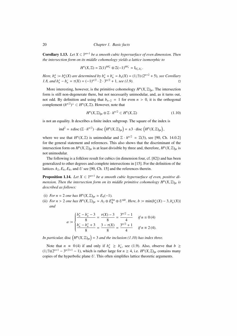
20 Chapter 1. Basic facts
Corollary 1.13. Let X ⊂ Pn+1 be a smooth cubic hypersurface of even dimension. Thenthe intersection form on its middle cohomology yields a lattice isomorphic to
Hn(X,Z) ' Z(1)⊕b+n ⊕ Z(−1)⊕b−n ' Ib+
n ,b−n .
Here, b±n B b±n (X) are determined by b+n + b−n = bn(X) = (1/3) (2n+2 + 5), see Corollary
1.8, and b+n − b−n = τ(X) = (−1)n/2 · 2 · 3n/2 + 1, see (1.9).
More interesting, however, is the primitive cohomology Hn(X,Z)pr. The intersectionform is still non-degenerate there, but not necessarily unimodular, and, as it turns out,not odd. By definition and using that bn−2 = 1 for even n > 0, it is the orthogonalcomplement (hn/2)⊥ ⊂ Hn(X,Z). However, note that
Hn(X,Z)pr ⊕ Z · hn/2 ⊂ Hn(X,Z) (1.10)
is not an equality. It describes a finite index subgroup. The square of the index is
ind2 = ±disc (Z · hn/2) · disc(Hn(X,Z)pr
)= ±3 · disc
(Hn(X,Z)pr
),
where we use that Hn(X,Z) is unimodular and Z · hn/2 ' Z(3), see [90, Ch. 14.0.2]for the general statement and references. This also shows that the discriminant of theintersection form on Hn(X,Z)pr is at least divisible by three and, therefore, Hn(X,Z)pr isnot unimodular.
The following is a folklore result for cubics (in dimension four, cf. [82]) and has beengeneralized to other degrees and complete intersections in [15]. For the definition of thelattices A2, E6, E8, and U see [90, Ch. 15] and the references therein.
Proposition 1.14. Let X ⊂ Pn+1 be a smooth cubic hypersurface of even, positive di-mension. Then the intersection form on its middle primitive cohomology Hn(X,Z)pr isdescribed as follows:
(i) For n = 2 one has Hn(X,Z)pr ' E6(−1).(ii) For n > 2 one has Hn(X,Z)pr ' A2 ⊕ E⊕a
8 ⊕ U⊕b. Here, b B minb+n (X) − 3, b−n (X)
and
a B
b+
n − b−n − 38
=τ(X) − 3
8=
3n/2 − 14
if n ≡ 0 (4)
b−n − b+n + 3
8=
3 − τ(X)8
=3n/2 + 1
4if n ≡ 2 (4).
In particular, disc(Hn(X,Z)pr
)= 3 and the inclusion (1.10) has index three.
Note that n ≡ 0 (4) if and only if b+n ≥ b−n , see (1.9). Also, observe that b ≥
(1/3)(2n+1 − 3n/2+1 − 1), which is rather large for n ≥ 4, i.e. Hn(X,Z)pr contains manycopies of the hyperbolic plane U. This often simplifies lattice theoretic arguments.

1 Numerical and cohomological invariants 21
Proof Assume n > 2, so that b+n (X) > 3, and consider the odd, unimodular lattice
Λ B Z⊕3 ⊕ E⊕a8 ⊕ U⊕b.
It has rank rk(Λ) = bn(X) and signature τ(Λ) = τ(X).1 Therefore, Λ and Hn(X,Z) areodd, indefinite, unimodular lattices of the same rank and signature and hence isomorphicto each other (and to Ib+
n ,b−n ), cf. [141, V. Thm. 6].Recall that a primitive vector α ∈ Λ in an odd unimodular lattice Λ is called charac-
teristic if (α.β) ≡ (β)2 (2) for all β ∈ Λ. Obviously, the orthogonal complement α⊥ ⊂ Λ
of a characteristic class is always even. The converse also holds, cf. [112, Lem. 3.3].Indeed, for any primitive α ∈ Λ in the unimodular lattice Λ there exists β0 ∈ Λ with(α.β0) = 1. Then for all β ∈ Λ the class β − (α.β) β0 is contained in α⊥ and in particu-lar of even square if α⊥ is assumed to be even. Hence, (β)2 ≡ (α.β)2 (β0)2 (2). As Λ isodd, there exists a β with (β)2 odd and hence (β0)2 must be odd. Altogether this proves(β)2 ≡ (α.β)2 ≡ (α.β) (2) for all β, i.e. α is characteristic.
For example, (1, 1, 1) ∈ Z⊕3 is characteristic, for its orthogonal complement is A2.In this case it can also be checked directly by observing that ((1, 1, 1).(x1, x2, x3)) =
x1 + x2 + x3 ≡ x21 + x2
2 + x23 = ((x1, x2, x3))2 (2). But then (1, 1, 1) ∈ Λ is also characteristic
and its orthogonal complement is the lattice in (ii).One now applies a general result for unimodular lattices from [157, Thm. 3]: Two
primitive vectors α, β ∈ Λ are in the same O(Λ)-orbit if and only if (α)2 = (β)2 and areeither both characteristic or both not.
Therefore, to prove the assertion, it suffices to show that hn/2 ∈ Hn(X,Z) is charac-teristic or, equivalently, that Hn(X,Z)pr is even. We postpone the proof of this statementto Corollary 2.11, where it fits more naturally in the discussion of Picard–Lefschetztheory and of the monodromy action of the universal family of hypersurfaces. A moretopological argument is given in [112].
It remains to deal with the case n = 2, where we have H2(X,Z) ' I1,6. It is easyto check that α B (3, 1, . . . , 1) ∈ I1,6 is characteristic with (α)2 = 3 and its orthog-onal complement turns out to be E6(−1) ' α⊥ ⊂ I1,6. Indeed a computation showsthat e1 B (0, 1,−1, 0, 0, 0, 0), e2 B (0, 0, 1,−1, 0, 0, 0), e3 B (0, 0, 0, 1,−1, 0, 0), e4 B
(1, 0, 0, 0, 1, 1, 1), e5 B (0, 0, 0, 0, 1,−1, 0), and e7 B (0, 0, 0, 0, 1,−1) span α⊥ and thattheir intersection matrix is just E6(−1).
Now consider the class of the hyperplane section h ∈ H2(X,Z). As in this casePic(X) ' H2(X,Z), one can argue algebraically, using the Hirzebruch–Riemann–Rochformula, to prove that h is characteristic. Indeed,
χ(X, L) =(L.L) + (L.h)
2+ 1
1 Note that τ ≡ 3 (8) is a general fact for unimodular lattices containing a characteristic element α with(α)2 ≡ 3 (8), cf. [141, V. Thm. 2]). In our situation, τ(X) ≡ 3 (8) can be deduced from (1.9).

22 Chapter 1. Basic facts
implies (L.h) ≡ (LL) ≡ 0 (2). Hence, using [157, Thm. 3] again, H2(X,Z)pr ' α⊥ '
E6(−1).Later we will describe the isomorphisms H2(X,Z)pr ' E6(−1) from a more geometric
perspective and, in particular, write down bases of both lattices in terms of lines, seeSections 4.1-3.
Remark 1.15. In [104, Thm. 11.1] it is shown that the purely lattice theoretic descrip-tion in Corollary 1.13 of the intersection product on Hn(X,Z) can be realized geomet-rically in the following sense: For n ≡ 0 (4) a smooth cubic hypersurface X ⊂ Pn+1
is diffeomorphic to a connected sum of the form M#k(S n × S n) with k = b−n (X) and,therefore, bn(M) = τ(X). For n ≡ 2 (4), n ≥ 4 the hypersurface is diffeomorphicto a connected sum of the form M#k(S n × S n) with k = b+
n (X) − 1 and, therefore,bn(M) = −τ(X) + 2.
For n ≡ 1 (2), a smooth cubic hypersurface X is diffeomorphic to M#k(S n × S n), withk = bn(X)/2 − 1 and, hence, bn(M) = 2. For n = 1, 3, or 7 this can be improved tok = bn(X)/2 and bn(M) = 0.
The remaining case of smooth cubic surfaces X ⊂ P3 is slightly different. Viewing Xas the blow-up of P2 in six points (see Section 4.2.2) reveals that it is diffeomorphic tothe connected sum P2#6P2.
1.6 We conclude with a number of comments on (cubic) hypersurfaces over arbitraryfields and notably in positive characteristics. Most of the subtleties and pathologies thatusually occur for varieties over fields of positive characteristic can safely be ignored forhypersurfaces. In the following, let X ⊂ Pn+1
k be a smooth hypersurface over an arbitraryfield k.
(i) The Hodge–de Rham spectral sequence
Ep,q1 = Hq(X,Ωp
X) +3 Hp+qdR (X/k) (1.11)
degenerates, cf. Section 4.6. For char(k) = 0 or char(k) > dim(X), this followsfrom [51]. Indeed, smooth hypersurfaces over fields of positive characteristic canof course be lifted to characteristic zero.
More directly and avoiding the assumption char(k) > dim(X), one can argueas follows. The computations above show in particular that the Hodge numbershp,q(X) = dim(Ep,q
1 ) of smooth hypersurfaces only depend on d and n, but not onchar(k). From (1.11) one deduces that
∑p+q=m hp,q(X) ≥ dim H,
dR(X/k). Moreover,equality holds if and only if the spectral sequence degenerates. On the other hand,dim Hm
dR(X/k) is upper semi-continuous. Hence, the degeneration of the spectralsequence in characteristic zero implies the degeneration in positive characteristic.
(ii) The Kodaira vanishing Hq(X,ΩpX ⊗ L) = 0 for p + q > n and L ∈ Pic(X) ample

2 Linear system and Lefschetz pencils 23
holds. This can either be seen as a consequence of [51] for large enough character-istic or read off from Corollaries 1.4 and 1.6. In particular, all numerical assertionson Hodge numbers remain valid over arbitrary fields. Also, for algebraically closedfields, the étale Betti numbers equal the ones computed in characteristic zero. Theonly case not covered by these comments is the case of cubic surfaces in charac-teristic two.
(iii) Assume k = Fq. Then the Weil conjectures show that
Z(X, t) B exp
∞∑r=1
|X(Fqr )|tr
r
=P(t)(−1)n+1∏ni=0(1 − qit)
with P(t) =∏
(1 − αit) of degree bn(X)pr and αi algebraic integers of absolutevalue |αi| = qn/2. In fact, this was established by Bombieri and Swinnerton-Dyer[22] for cubic threefolds and by Dwork [58] for arbitrary hypersurfaces, prior tothe proof of the general Weil conjectures by Deligne. Of course, as cubic surfacesare rational, the Weil conjectures follow from the Weil conjectures for P2 and forcurves.
2 Linear system and Lefschetz pencils
This section discusses the linear system of (cubic) hypersurfaces. Basic facts concerningthe discriminant divisor are reviewed and, in particular, its degree is computed. Wedescribe the monodromy group of the family of smooth hypersurfaces as a subgroupof the orthogonal group of the middle cohomology and complement the results with acomparison of the action of the group of diffeomorphisms.
Hypersurfaces X ⊂ P = Pn+1 of degree d are parametrized by the projective space
|O(d)| ' PN(d,n),
where N = N(d, n) = h0(Pn+1,O(d))− 1 =(
n+1+dd
)− 1. The universal hypersurface shall
be denoted
X ⊂ PN × P. (2.1)
It is of bidegree (1, d), i.e. a divisor contained in the linear system |OPN (1)OP(1)|, andthe fibre of the (flat) first projection X // PN over the point corresponding to X ⊂ P isindeed just X.
More explicitly, X can be described as the zero set of the universal equation G =∑aI xI , where aI ∈ H0(PN ,OPN (1)) are the linear coordinates corresponding to the
monomials xI ∈ H0(P,OP(d)). In other words, if one writes P as P = P(V) for somevector space V of dimension n + 2, then H0(P,O(d)) = S d(V∗) and PN = P(S d(V∗)).

24 Chapter 1. Basic facts
Hence, H0(PN ,OPN (1)) = S d(V) and then G corresponds to the identity in End(S d(V)) 'S d(V) ⊗ S d(V∗) = H0(PN × P,OPN (1) OP(d)).
The universal hypersurface X is smooth. For this observe that the second projectionX // P is the projective bundle P(Ker(ev)) // P, where ev is the evaluation map
ev: H0(P,O(d)) ⊗O // //O(d).
2.1 The natural SL(n + 2)-action on H0(P,O(d)) descends to an action of SL(n + 2)and PGL(n + 2) on |OP(d)|. Both are linearized in the sense that they are obtained bycomposing homomorphisms SL(n + 2) // SL(N + 1) and PGL(n + 2) // PGL(N + 1)with the natural actions of SL(N + 1) and PGL(N + 1) on H0(PN ,OPN (1)) and |OPN (1)|.
The following table records the dimensions of the linear system of cubic hypersur-faces of small dimensions. It also contains information about the moduli space
Mn B |OP(3)|sm/PGL(n + 2)
and the discriminant divisor D(n) B D(3, n) ⊂ |OP(3)|, both to be discussed below, seeSections 2.3 and 2.1.3. We write N(n) B N(3, n).
n N(n) dim(PGL(n + 2)) dim(Mn) deg(D(n))
0 3 3 0 41 9 8 1 122 19 15 4 323 34 24 10 804 55 35 20 1925 83 48 35 448
The closed formula for the dimension of the moduli space is
dim(Mn) =
(n + 2
3
)=
n3 + 3 n2 + 2 n6
. (2.2)
2.2 We are mostly interested in smooth hypersurfaces. They are parametrized by aZariski open subset which shall be denoted
U(n, d) B |OP(d)|sm B X ∈ |OP(d)| | X smooth ⊂ |OP(d)|.
For an algebraically closed ground field k, Bertini’s theorem shows that there exists asmooth hypersurface of the given degree d. Hence, U(n, d) is non-empty and, therefore,dense. In fact, if char(k) = 0 or at least char(k) - d, then the Fermat hypersurface
X = V
n+1∑i=0
xdi
⊂ P

2 Linear system and Lefschetz pencils 25
is always smooth, as it is easy to check using the Jacobian criterion. In [98, p. 333] onefinds the following explicit equations for smooth hypersurfaces over arbitrary fields
∑m−1i=0 xi xi+m if d = 2, n + 2 = 2m∑m−1i=0 xi xi+m + x2
n+1 if d = 2, n + 1 = 2m∑n+1i=0 xd
i if d ≥ 3, char(k) - d∑ni=0 xi xd−1
i+1 + xd0 if d ≥ 3, char(k) | d.
(2.3)
Hence, the set of k-rational points of U(n, d) = |OP(d)|sm is always non-empty.
Definition 2.1. The discriminant divisor D(d, n) ⊂ |OP(d)| is the complement of theZariski open (and dense) subset U(d, n) ⊂ |OP(d)| of smooth hypersurfaces. Thus,D(d, n) is closed and it will be viewed with its reduced induced scheme structure.
Theorem 2.2. The discriminant divisor D(d, n) ⊂ |OP(d)| is an irreducible divisor. Itsdegree is (d − 1)n+1 (n + 2), which for d = 3 reads
deg(D(3, n)) = 2n+1 (n + 2).
Proof Consider the universal hypersurface X ⊂ PN × P as above and define
Xsing B X ∩n+1⋂i=0
Vi,
where the Vi B V(∂iG) are the hypersurfaces of bidegree (1, d − 1) defined by thederivatives of the equation of the universal hypersurface
∂iG B∑
aI∂xI
∂xi∈ H0
(PN × P,OPN (1) OP(d − 1)
).
By the Jacobian criterion, Xsing ⊂ X // PN is the family of singular loci of the fibresXt, i.e. (Xsing)t = (Xt)sing.
As the Euler equation (see [24, Ch. 4]) holds in its universal form∑
xi ∂iG = d·G, onehas X ⊂
⋂Vi if char(k) - d (which we will tacitly assume, but see Remark 2.3). Hence,
Xsing =⋂
Vi and, therefore, codim(Xsing) ≤ n+2. To prove that equality holds, considerthe other projection Xsing // P, which we claim is a Pk-bundle with k = N − n − 2. Tosee this, observe that the homomorphism of sheaves on P
ϕ : H0 (P,OP(d)) ⊗OP //O(d − 1)⊕n+2, F // (∂iF)
is surjective, which can be checked e.g. at the point z = [1 : 1 : · · · : 1] by using that(∂ixd
j )(z) = d · δi j, and
Xsing ' P(Ker(ϕ)) // P.
This clearly proves codim(Xsing) = n + 2, but also that Xsing is smooth and irreducible.

26 Chapter 1. Basic facts
To be precise, one needs to verify that Xsing ' P(Ker(ϕ)) as schemes and not only assets, which is left to the reader.
Next, D B D(d, n) is by definition the image of Xsing under the projection
Xsing ⊂ X ⊂ PN × P // PN .
Let us denote the pull-backs of the hyperplane sections on PN and P (both denoted byh) to PN ×P by h1 and h2. Suppose D is of codimension > 1. Then (hN−1.D) = 0, which,however, would contradict
(hN−11 .Xsing) = (hN−1
1 .(h1 + (d − 1) h2)n+2) = (n + 2) (d − 1)n+1.
Hence, D ⊂ PN really is a divisor. The computation also shows that in order to provethe claimed degree formula for D, it suffices to prove that Xsing // // D is generically in-jective or, in other words, that the generic singular hypersurface X ∈ |OP(d)| has exactlyone singular point (which is in fact an ordinary double point). (One needs to assumechar(k) = 0 for the set-theoretic injectivity to imply that the morphism is of degreeone.) One way of doing it would be to write down examples of hypersurface in eachdegree with exactly one ordinary double point2 or to argue geometrically (assumingchar(k) = 0) by considering again the projective bundle Xsing // P. The fibre over apoint z can be thought of as a linear system with z as its only base point. By Bertini’stheorem with base points, see e.g. [80, III. Rem. 10.9.2], the generic element will thenbe singular exactly at z. To see that generically it has to be an ordinary double point, justwrite down one hypersurface with such a singular point at z (but possibly other singularpoints), e.g. the union of (d − 2) generic hyperplanes Pn ⊂ P and of a cone with vertexz over a quadric in some hyperplane.
Remark 2.3. In [1, Exp. XVII] the discriminant divisor is viewed as the dual variety ofthe Veronese embedding νd : P
// PN , i.e. as the locus of hyperplanes (parametrizedby PN) that are tangent to νd(P). It is also proved that the smooth locus of D(d, n) isthe maximal open subset over which Xsing // // D(d, n) is an isomorphism and that itcoincides with the set of those singular hypersurfaces with one ordinary double point asonly singularity.
2.3 There is a classical and more algebraic approach to the discriminant divisor usingresultants, cf. [28, 40, 52, 67]. Here are some general facts. Consider homogeneouspolynomials in k[x0, . . . , xn+1] of degree di > 0, i = 0, . . . ,m. Then there exists a uniquepolynomial, the resultant, R(yi,I) B Rd,n(yi,I) ∈ k[yi,I], i = 0, . . . ,m, |I| = di, such that:
(i) For all fi ∈ k[x0, . . . , xn+1]di , i = 0, . . . ,m, the intersection⋂
V( fi) ⊂ Pn+1k
is non-empty if and only if R( f0, . . . , fm) = 0.
2 Duco van Straten has provided me with examples in certain degrees. Note that writing down exampleswith just one singular point is easy, e.g. the cone over the smooth examples in (2.3) has only one singularpoint, which however is an ordinary double point only for d = 2.

2 Linear system and Lefschetz pencils 27
(ii) R(xd00 , . . . , x
dmm ) = 1 (normalization).
(iii) R ∈ k[yi,I] is irreducible.
In (i), R( f0, . . . , fm) is the shorthand for applying R to the coefficients of the polyno-mials fi. Moreover, R is homogeneous of degree
∏j,i d j in the variables yi,I for fixed i
and so of total degree∏
di ·∑
(1/di).Consider F ∈ k[x0, . . . , xn+1] and apply the above to fi = ∂iF, i = 0, . . . ,m = n + 2,
which are all homogeneous of degree di = d − 1. Then X = V(F) is singular, i.e.⋂V( fi) , ∅, if and only X ∈ |O(d)| is in the zero locus of R.Strictly speaking, R defines a hypersurface in PN′ = Proj(k[yi,I]), i = 0, . . . , n + 1,
|I| = d − 1, so N′ = (n + 2)(
n+dd−1
)− 1. Its pull-back via the linear embedding PN // PN′
that maps xI to[i jxI j
]j=0,...,n+1
, where for I = (i0, . . . , in+1) one sets I j B (i0, . . . , (i j −
1), . . . , in+1), describes the image of Xsing, i.e. the discriminant divisor. The irreducibilitystill holds, cf. [52, Sec. 5&6].
D(d, n) = V(Rd,n (∂0G, . . . , ∂n+1G)) ⊂ PN = |OP(d)|.
Remark 2.4. The resultant is usually normalized to yield the discriminant
∆d,n B dcd,n · Rd,n(∂iG) ∈ H0(PN ,OPN ((d − 1)n+1(n + 2))
), (2.4)
where cd,n = (1/d) ((−1)n+2 − (d − 1)n+2). With this normalization, ∆d,n becomes anirreducible polynomial in Z[yI], which makes it unique up to ±1.
Example 2.5. The case n = 0 and d = 3, so three points in P1, leads to the classicaldiscriminant for cubic polynomials f (X). If α1, α2, α3 are the zeros of f (X), then bydefinition ∆( f (X)) = ((α1 − α2) (α1 − α3) (α2 − α3))2. For f (X) = X3 + aX + b one has∆( f (X)) = −4a3 − 27b2.
The discriminant of a general polynomial a0x30 + a1x2
0x1 + a2x0x21 + a3x3
1 is the rathercomplicated polynomial of degree four
∆3,0 = a21a2
2 − 4a3a31 − 4a3
2a0 − 27a23a2
0 + 18a0a1a2a3,
which thus defines the discriminant surface
D(3, 0) = V(∆3,0) ⊂ P3.
As an exercise, the reader may want to compare this with the normalization R(x20, x
21) =
1, which in (2.4), using c3,0 = −1, yields ∆3,0
((1/3) (x3
0 + x31))
= (1/3).To confirm Remark 2.3, the reader may want to verify that singular set of D(3, 0) =
V(∆3,0) is indeed the curve of triple points.
Example 2.6. For n = 1 and d = 3 the discriminant divisor
D(3, 1) ⊂ P9

28 Chapter 1. Basic facts
is of degree 12 or, equivalently, the discriminant is an element of the vector spaceH0(P9,OP9 (12)), which is of dimension 293.930. Written as a linear combination ofmonomials, 12.894 of the coefficients are non-trivial, cf. [40, p. 99]. If the partial deriva-tives ∂iF are written as ∂0F = a11x2
0 + a12x21 + a13x2
2 + a14x0x1 + a15x0x2 + a16x1x2, etc.,and one defines [`1`2`3] B det (ai,` j ) ∈ H0(P9,O(3)), with pairwise distinct `i, then∆ is a polynomial of degree four in the [`1`2`3] involving only 68 terms. In short, thediscriminant is complicated.
Maybe just one word on the comparison between the discriminant introduced hereand the discriminant of a plane cubic E ⊂ P2 in Weierstrass form y2 = 4x3 − g2x − g3
which is classically defined as ∆(E) B g32 − 27g2
3. This is a rather simple polynomialof degree three in the coefficients, whereas the full discriminant of cubic plane curvesis a polynomial of degree 12. The reason for this is that bringing a cubic polynomial inthe variables x0, x1, x2 into Weierstrass form involves non-linear transformations. Moreconcretely, the coefficients g2 and g3 of the Weierstrass form are of degree four and six,respectively, in the coefficients of the original cubic equation, see e.g. [99, Ch. 3].
As a consequence of Theorem 2.2 and the discussion in its proof, we deduce thefollowing.
Corollary 2.7. Assume k = k. Then for the generic line P1 // PN the induced familyXP1 // P1 has exactly (d − 1)n+2 (n + 2) singular fibres X1,X2, . . ., each with exactlyone singular point xi ∈ Xi. Moreover, the xi are all ordinary double points.
A pencil with these properties is called a Lefschetz pencil. Note that by Bertini’stheorem [80, III. Cor. 10.9], at least when char(k) = 0, the total space XP1 is still smooth.See [1, Exp. XVII].
In more concrete terms, for generic choice of polynomials F0, F1 ∈ H0(P,O(d)) forexactly (d − 1)n+2 (n + 2) values t = [t0 : t1] the hypersurface Xt = V(t0 F0 + t1 F1) issingular. Each singular fibre Xi has exactly one singular point xi, which, moreover, is anordinary double point. Note that xi , x j for i , j, as otherwise xi would be a singularpoint of all the fibres.
Example 2.8. There are, of course, pencils XP1 // P1 // PN with more singular fi-bres, e.g. with more or worse singularities. The Hesse pencil of plane cubics Xt ⊂ P
2
given by
t0 (x30 + x3
1 + x32) + t1 x0x1x2
is such an example. Here, the fibre X[0:1] consists of three lines yielding three singularpoints. The Hesse pencil is a special instance of the Dwork pencil (or Fermat pencil),

2 Linear system and Lefschetz pencils 29
see [19], defined by the equation
t0
n+1∑i=0
xn+2i
− t1 dn+1∏i=0
xi
of hypersurfaces of degree d = n + 2.Clearly, the number of singular fibres of any pencil is bounded by (d − 1)n+1 (n + 2),
unless all fibres are singular. Note that for general pencils the total space XP1 need notbe smooth.
2.4 We now assume k = C. Let us consider the universal family of smooth hypersur-faces
π : X //U(d, n) ⊂ |OPn+1 (d)|.
Note the change in notation. If needed later, we will denote the universal family ofall hypersurfaces by X . It is smooth and projective and contains X as a dense opensubset. Fix a point 0 ∈ U(d, n) and denote the fibre over it by X B X0. The monodromyrepresentation
ρ : π1(U(d, n), 0) //GL(Hn(X,Z)) (2.5)
is the homomorphism obtained by parallel transport with respect to the Gauss–Maninconnection. Equivalently, Rnπ∗Z is a locally constant system on U(n, d) and (2.5) is thecorresponding representation of the fundamental group. The monodromy group is bydefinition the image of the monodromy representation
Γ(d, n) B Im (ρ : π1(U(d, n), 0) //GL(Hn(X,Z)))
and it depends on 0 ∈ U(d, n) only up to conjugation.The monodromy group has been determined in [12] in complete generality. We state
the result for d = 3 and use the shorthand
Γn B Γ(3, n) ⊂ GL(Hn(X,Z)).
Theorem 2.9. The monodromy group Γn of the universal smooth cubic hypersurfaceX // |OPn+1 (3)|sm is the group
Γn '
O+(Hn(X,Z)) if n ≡ 0 (2)
SpO(Hn(X,Z), q) if n ≡ 1 (2).
In fact, [12] shows that Γ(d, n) for n even and arbitrary d and for n odd and for all oddd admits the description. If n and d are both odd, then the monodromy group is the fullsymplectic group Sp(Hn(X,Z)).
Before sketching the main steps of the proof, let us explain the notation: For n even,

30 Chapter 1. Basic facts
one defines O(Hn(X,Z)) ⊂ O(Hn(X,Z)) as the subgroup of all orthogonal transfor-mations g : Hn(X,Z) ∼
− // Hn(X,Z) with g(hn/2) = hn/2. Via the induced action onHn(X,Z)pr it can be identified with the subgroup (cf. [90, Prop. 14.2.6])
O(Hn(X,Z)) '
g ∈ O(Hn(X,Z)pr) | id = g ∈ O(AHn(X,Z)pr ).
Here, we use the notation AΛ B Λ∗/Λ for the discriminant of a lattice Λ, which for theprimitive cohomology of a smooth cubic hypersurface is just Z/3Z.
Another subgroup is given as
O+(Hn(X,Z)pr) B Ker(snn : O(Hn(X,Z)pr) // ±1
).
Here, the spinor norm snn(sδ) of a reflection in δ⊥ is defined as (−1)n/2 · (δ)2/|(δ)2|. Inother words, if g is written as a product
∏sδi of reflections with δi ∈ Hn(X,R)pr (using
the Cartan–Dieudonné theorem), then snn(g) = 1 if the number of δi with (δi)2 < 0 forn ≡ 0 (4) (respectively, of δi with (δi)2 > 0 for n ≡ 2 (4)) is even.
The orthogonal group in the theorem is the finite index subgroup of O(Hn(X,Z)pr):
O+(Hn(X,Z)) B O(Hn(X,Z)) ∩ O+(Hn(X,Z)pr).
In fact, O+(Hn(X,Z)) = O(Hn(X,Z)) for d = 3 and n , 2, see [].For n odd, the intersection product on Hn(X,Z) = Hn(X,Z)pr is alternating and can
be put in the standard normal form. However, there exists an auxiliary rather subtletopological invariant, which is the quadratic form q : Hn(X,Z) // Z/2Z (see [27, Sec.1]) that enters the definition of the group SpO(Hn(X,Z), q) in the above theorem. Usingthat any α ∈ Hn(X,Z) can be represented by an embedded sphere S n // X, one hasfor n , 1, 3, 7 that q(α) = 0 if and only if the topological normal bundle of S n // Xis trivial. 3 The definition for n = 1, 3, 7 is more involved. Then SpO(Hn(X,Z), q) isdefined as the group of isomorphisms g : Hn(X,Z) ∼
− // Hn(X,Z) compatible with thealternating intersection form ( . ) and the quadratic form q.
Remark 2.10. The appearance of the primitive cohomology in Theorem 2.9 is not asurprise. Indeed, the restriction of hn/2 = c1(O(1))n/2 ∈ Hn(Pn+1,Z) to any of the fibresXt defines a section of the locally constant system Rnπ∗Z. Hence, the primitive co-homology groups Hn(Xt,Z)pr of the fibres glue to a locally constant subsheaf Rn
prπ∗Z ⊂
Rnπ∗Z. Equivalently, the monodromy representation (2.5) satisfies ρ(γ)(hn/2) = hn/2 forall γ ∈ π1(U(d, n)), i.e. hn/2 is monodromy invariant.
In fact, hn/2 is the only monodromy invariant class up to scaling. Indeed, Deligne’sinvariant cycle theorem [154, V. Thm. 16.24] shows that the monodromy invariant part
3 The Arf invariant of q, also called the Kervaire invariant of X, is often viewed as the analogue of thediscriminant of the symmetric intersection form for n even. Recall that the Arf invariant A(q) ∈ F2 of thebinary quadratic form q = ax2 + xy + by2 is ab. For arbitrary q, which can be written as a direct sum ofthose, it is defined by additive extension, cf. [26, Ch. III]. Due to [104, Prop. 12.1], the Kervaire invariantis non-trivial for cubic hypersurfaces

2 Linear system and Lefschetz pencils 31
of Hn(X,Q)ρ ⊂ Hn(X,Q) is the image of the restriction Hn(X ,Q) // Hn(X,Q), whereX ⊂ PN × P denotes the universal family of all hypersurfaces. Now writing X as a pro-jective bundle over P shows that Hn(X ,Q) '
⊕Hn−2i(P,Q)·c1(OPN (1))i. As c1(OPN (1))
restricts trivially to the fibres of the first projection X // PN , only Hn(P,Q) survivesthe map Hn(X ,Q) // Hn(X,Q) and, therefore, its image is spanned by hn/2.
Similarly, the monodromy representation preserves the intersection form on Hn(X,Z).Therefore, Im(ρ) ⊂ O(Hn(X,Z)) for n even and Im(ρ) ⊂ Sp(Hn(X,Z)) for n odd.
Note that one can deduce from the theorem the well-known fact [154, V. Thm. 15.27]that Hn(X,Q)pr is an irreducible Γ(d, n)-module or, equivalently, that Rn
prπ∗Q cannot bewritten as a direct sum of non-trivial locally constant systems.
2.5 The computation of the monodromy group Γn, or more generally of Γ(d, n), pro-ceeds in three steps.
(i) Show that Γ(d, n) equals the monodromy group of the smooth part of a Lefschetzpencil XP1 // P1.
(ii) Assume X // ∆ is a family of hypersurfaces over a disk with X and Xt,0 smoothand such that the central fibre X0 has one ordinary double point as its only singu-larity. Let γ be the simple loop around 0 ∈ ∆. Describe the induced monodromyoperation ρ(γ) : Hn(X,Z) ∼
− // Hn(X,Z), where X = Xε is a distinguished smoothfibre, as a reflection sδ.
(iii) Let XP1 // P1 be a Lefschetz pencil with nodal singular fibres over t1, . . . , t` ∈P1 \∞. Describe the sub-group 〈sδi〉 ⊂ GL(Hn(X,Z)) generated by the monodromyoperations around all the nodal fibres Xt1 , . . . ,Xt` .
To give at least a rough idea, here are a few more details for all three steps. For detailsof the statements and proofs we have to refer to the literature, cf. [154].
(i) Similar to the Lefschetz hyperplane theorem for smooth hyperplane sections ofsmooth projective varieties, cf. Section 1.1, a result of Zariski, see [77] or [154, V. Thm.15.22], shows that for a very general line P1 ⊂ PN = |O(d)| the induced map
π1(P1 \ D) // // π1(PN \ D) (2.6)
is surjective. (From now on we suppress the base point in P1 ⊂ PN in the notation.) Therestriction of Rnπ∗Z to P1 \ D, which is isomorphic to the higher direct image for therestriction of the family to P1 \ D, corresponds to the representation
π1(P1 \ D) // // π1(PN \ D) //GL(Hn(X,Z))
obtained by composing (2.5) with (2.6). Hence, Γ(d, n) can be computed as the mono-dromy group of an arbitrary Lefschetz pencil XP1 // P1, i.e. as the image of
ρP1 : π1(P1 \ D) //GL(Hn(X,Z)). (2.7)

32 Chapter 1. Basic facts
By Theorem 2.2, P1 \ D ' P1 \ t1, . . . , t` with ` = (d − 1)n+1 (n + 2). Therefore,π1(P1 \ D) is isomorphic to a quotient of the free group π1(C \ t1, . . . , t`) ' Z∗` withfree generators given by the simple loops γi around the points ti ∈ C. Thus, in orderto describe the image of (2.7), we need to compute the monodromy operators ρP1 (γi)and the group they generate. (In our discussion the details concerning the base pointand the dependence on the path connecting it to circles around the critical values aresuppressed.)
(ii) Let x ∈ X0 be the ordinary double point of the central fibre of a family X // ∆obtained from the above by restriction to a small disk ∆
// P1, 0 // ti. Intersectinga ball B(x) ⊂ X around x with the nearby smooth fibre X = Xε retracts to a sphereS n ⊂ B(x) ∩ X ⊂ X. It is called the vanishing sphere and its cohomology class δ =
[S n] ∈ Hn(X,Z) is the vanishing class. Its main property, responsible for its name andverified by a local computation, is that it generates the kernel of the push-forward map(cf. [154, V. Cor. 14.17]):
Hn(X,Z) ' Hn(X,Z) // Hn(X ,Z).
The self intersection (δ)2, determined by the normal bundle of S n ⊂ X, is given by
(δ)2 =
0 if n ≡ 1 (2)
−2 if n ≡ 2 (4)
2 if n ≡ 0 (4).
Of course, the vanishing for odd n follows from the fact that in this case the intersectionpairing on the middle cohomology is alternating. The other two cases are obtained byan explicit computation, see [154, IV.15.2].
The crucial input is the description of the monodromy operation ρ(γ) induced by asimple loop around 0 ∈ ∆. It is described by the Picard–Lefschetz formula:
ρ(γ) = sδ : α // α + εn (α.δ) δ, (2.8)
where
εn =
1 if n ≡ 2, 3 (4)
−1 if n ≡ 0, 1 (4),
i.e. εn = −(−1)n(n−1)/2. Note that the sign is such that for n even sδ is a reflection in δ⊥
and so, in particular, sδ(δ) = −1 and s2δ = id. For n odd, the monodromy is not of finite
order, as skδ(α) = α + εn k (α.δ) δ.4
(iii) We have computed the images ρP1 (γi) of the free loops around the singular fibres
4 Note that in [12] the sign of the intersection form is changed for n ≡ 3 (4), so that in this case as wellsδ(α) = α + (α.δ) δ.

2 Linear system and Lefschetz pencils 33
Xti , i = 1, . . . , ` = deg D(d, n), as the operators sδi associated with the correspondingcorresponding classes δi. They are reflections for even n and of infinite order if n is odd.
Consider now families X i // ∆i around each ti ∈ P1 as in (ii). We may assumethat the smooth reference fibre is X for all of them. Note that all vanishing classesδi ∈ Hn(X,Z) are contained in the primitive cohomology. This follows from describingthe composition as the product with the hyperplane class
Hn(X,Z) ' Hn(X,Z) // Hn(X i,Z) // Hn(P,Z) ' Hn+2(P,Z) // Hn+2(X,Z).
In fact, the vanishing cohomology Hn(X,Z)van B Ker(Hn(X,Z) // Hn+2(P,Z)), whichin our situation coincides with the primitive cohomology, is generated over Z by thevanishing classes, see [154, V. Lem. 14.26] or for the algebraic treatment [50, Sec. 4.3].This has the following consequence.
Corollary 2.11. The primitive cohomology Hn(X,Z)pr of a smooth hypersurface X ⊂Pn+1 is generated by classes δ with (δ)2 even and, in fact, (δ)2 = −2, 0, 2 for n ≡ 2 (4),n ≡ 1 (2), and n ≡ 0 (4), respectively. In particular, for n ≡ 0 (2), the lattice Hn(X,Z)pr
is even.
Note that the fact that Hn(X,Z)pr is generated by the vanishing classes δi in partic-ular shows that bn(X)pr ≤ deg D(d, n), which is confirmed by a quick comparison ofCorollary 1.8 with Theorem 2.2.
For even n the Weyl group
W ⊂ O(Hn(X,Z)pr)
is by definition the subgroup generated by the reflections sδi . For n odd the Weyl groupW ⊂ Sp(Hn(X,Z)) is defined analogously. It turns out, that in both cases it acts tran-sitively on the set of vanishing classes ∆ B δi, cf. [113, Prop. 7.5] or [154, Prop.15.23].
A lattice Λ (symmetric or alternating) with a class of vectors ∆ ⊂ Λ generating Λ andwith the associated Weyl group acting transitively on ∆ is called a vanishing lattice, see[59, 97]. By our discussion so far we have
Γ(d, n) = Im(ρ) = Im(ρP1 ) = W.
The proof of Theorem 2.9 for even n > 2 is in [12] reduced to a purely lattice theoreticresult in [59] describing the Weyl group of a complete vanishing lattice as this particu-lar subgroup of the orthogonal group of the lattice. The lattice Hn(X,Z)pr is complete,which means that ∆ contains a certain configuration of six vanishing classes. The factthat for n > 2, in accordance with Proposition 1.14, the lattice contains A2 ⊕U⊕2 is partof the picture. The case of cubic surfaces is well known classically and is usually statedas
Γ(3, 2) ' W(E6).

34 Chapter 1. Basic facts
This is the only case of cubic hypersurfaces in which the monodromy group is actuallyfinite. Indeed, it is an index two subgroup of the finite orthogonal group O(H2(X,Z)pr)of the definite lattice H2(X,Z)pr. We shall come back to it in Section 4.1.3. For n oddthe result is deduced from [97].
Remark 2.12. In the algebraic setting, say over an algebraically closed field k, thegeometric monodromy group, i.e. the Zariski closure of the image of the representationπét
1 (U) //GL(Hn(X, Q`)), has been determined in [50, Sec. 4.4]. It is either a finitegroup for n = 2, the full orthogonal group O(Hn(X, Q`)pr) for n even and n > 2, or thefull symplectic group Sp(Hn(X, Q`)). For n even the proof comes down to the fact thatan algebraic subgroup G ⊂ O(V) of a complex vector space V with a non-degeneratesymmetric bilinear form is either finite or O(V). The latter case holds as soon as thereexists a G-orbit of classes δ with (δ)2 = 2 generating V and such that G contains allreflections sδ induced by classes in that orbit, cf. [50, Lem. 4.4.2].
Exercise 2.13. Consider the case n = 0 for which the universal smooth hypersurfaceX // P3 \ S , defined over the complement of a quartic surface S with the explicitequation given in Example 2.5, is an étale cover of degree three. Show that the mon-odromy group Γ(0, 3) is in fact S3. It equals the Galois group of the field extensionK(P3) ⊂ K(X ). See [78] for further information.
2.6 As any monodromy transformation is induced by a diffeomorphism, the mono-dromy group Γn is a subgroup of the image of the natural representation
τ : Diff+(X) //O(Hn(X,Z))
of the group of orientation preserving diffeomorphisms. It turns out that Im(τ) is slightlylarger than Γn. Details have been worked out in [12]. Here are the main steps.
Let us first consider the case that n is even and n > 2. Clearly, Diff+(X) also acts onH2(X,Z) ' Z · h and, therefore, sends h to h or to −h, where the latter is realized bycomplex conjugation defined on any X defined by an equation with coefficients in R. Asa consequence, Diff+(X) respects the direct sum decomposition Hn(X,Q) = Hn(X,Q)pr⊕
Q · hn/2. This eventually leads to
Im(τ) '
O(Hn(X,Z)) if n ≡ 0 (4)
O(Hn(X,Z)pr) if n ≡ 2 (4).
To prove this note that O+(Hn(X,Z)) ⊂ Im(τ) and that for n ≡ 2 (4) complex conjugationinduces an element in Im(τ) the restriction of which to Hn(X,Z)pr acts non-trivially onthe discriminant AHn
pr ' AZ·hn/2 ' Z/3Z. Hence, it is enough to find an orientation pre-serving diffeomorphism g which acts with spinor norm snn(τ(g)) = −1 on Hn(X,Z) andfixes hn/2. For this, one uses the connected sum decomposition of X as M′#(S n×S n), cf.Remark 1.15, and the diffeomorphism g obtained by gluing the identity on M′ with the

3 Automorphisms and deformations 35
product ι × ι of the diffeomorphism ι : S n // S n, (x1, . . . , xn+1) // (x1, . . . , xn,−xn+1).It acts on the induced orthogonal decomposition Hn(X,Z) ' Hn(M′,Z)⊕Hn(S n×S n,Z),for which we may assume that hn/2 ∈ Hn(M′,Z), by −id on Hn(S n × S n,Z) ' U and byid on U⊥ = Hn(M′,Z). Write −idU = se− f se+ f , with e, f ∈ U the standard basis, tosee that indeed snn(τ(g)) = −1 and τ(g)(hn/2) = hn/2.5
For cubic surfaces, there is no reason for a diffeomorphism to respect the hyperplaneclass (up to sign) and indeed Im(τ) = O(H2(X,Z)), cf. [158] and Section 4.1.3.
For n odd the result reads
Im(τ) =
SpO(Hn(X,Z), q) if n , 1, 3, 7
Sp(Hn(X,Z)) if n = 1, 3, 7.
Indeed, the description of q([S n]) for n , 1, 3, 7 in terms of the topological normalbundle of S n ⊂ X is invariant under diffeomorphisms. In the other cases one proves thatsδ is realized by a diffeomorphism for any primitive δ ∈ Hn(X,Z). As those generatethe symplectic group, this is enough to prove the claim for n = 1, 3, 7. Concretely, fora given δ, there exist δ′ with (δ.δ′) = 1 and a decomposition X ' M′#(S n × S n) withHn(S n × S n,Z) spanned by δ, δ′. In [12] it is then observed that the reflection sδ isrealized by gluing the identity on M′ with the diffeomorphism (x, y) // (x, x · y), wherex · y is the multiplication in C, H, or O for the three cases n = 1, 3, 7.
3 Automorphisms and deformations
Smooth hypersurfaces behave nicely in many respects. For example, for most of themthe deformation theory is easy to understand, not showing any of the pathologicalfeatures to be reckoned with for arbitrary smooth projective varieties. Similarly, theirgroup of automorphisms are usually finite and generically even trivial. We will assumed ≥ 3 throughout this section. The only slightly exotic cases that need special careare (n, d) = (1, 3) and (n, d) = (2, 4), i.e. plane cubic (elliptic) curves and quartic K3surfaces.
3.1 First order information about the group of automorphisms of a smooth hyper-surface X ⊂ Pn+1 and about its deformations are encoded by the cohomology groupsH0(X, TX) and H1(X, TX), respectively. Those can be computed in terms of the standardexact sequences. We begin, however, with the following well-known fact.
5 In [12] the result for n ≡ 2 (4) is stated as Im(τ) = O(Hn(X,Z))×±1. Indeed, complex conjugation definesan element of order two in Im(τ) that acts non-trivially on the discriminant of Hn(X,Z)pr. Moreover, itcommutes with the index two subgroup Γn = O+(Hn(X,Z)), as the universal family is defined over Rand hence monodromy commutes with complex conjugation. However, that complex conjugation alsocommutes with the additional diffeomorphism g seems to need an additional argument.

36 Chapter 1. Basic facts
Lemma 3.1. Assume char(k) - d. Then the hypersurface X ⊂ Pn+1 defined by F ∈k[x0, . . . , xn+1]d is smooth if and only if the partial derivatives ∂iF form a regular se-quence in k[x0, . . . , xn+1].
Proof A standard result in commutative algebra shows that a sequence ai ∈ A, i =
1, . . . , dim(A), in a regular local ring A is regular if and only if ht((ai)) = dim(A), cf.[118, Thm. 16.B]. Hence, (∂iF) is a regular sequence if and only if the affine intersectionV((∂iF)) =
⋂V(∂iF) ⊂ An+2 is zero-dimensional. However, as the polynomials ∂iF are
homogeneous, V((∂iF)) isGm-invariant. Hence, (∂iF) is a regular sequence if and only ifthe projective intersection V((∂iF)) ⊂ Pn+1 is empty. This implies that also X∩V((∂iF))is empty and, by the Jacobian criterion, that X is smooth. Conversely, if X is smooth andchar(k) - d, the Euler equation:
d · F =
n+1∑i=0
xi ∂iF. (3.1)
shows that V((∂iF)) = Xsing = ∅, i.e. (∂iF) is a regular sequence.
Example 3.2. The assumption on the characteristic is needed, as shown by the exampleF = x2
0x1 − x0x21 with char(k) = 3. Indeed, in this case X = 0,∞, [1 : 1] is smooth, but
∂0F = −x1 (x0 + x1) and ∂1F = x0 (x0 + x1) have a common zero in [1 : −1].
Corollary 3.3. Let X ⊂ P = Pn+1 be a smooth hypersurface of degree d.
(i) If n ≥ 0 and d ≥ 3 but (n, d) , (1, 3), then H0(X, TX) = 0.(ii) If n > 2 or d ≤ 3, then H1(X, TP|X) = 0 and the normal bundle sequence induces a
surjection
H0(X,OX(d)) // // H1(X, TX).
Proof We shall give a proof under the additional assumption that char(k) - d and referto [98, Sec. 11.7] for the general case.
Combining the Euler sequence 0 //OP //OP(1)⊕n+2 // TP // 0 and the normalbundle sequence 0 // TX // TP|X //OX(d) // 0, we obtain a diagram
H0(TP|X) // H0(OX(d)) // H1(TX) // H1(TP|X)
H0(OX(1))⊕n+2.
OO
(∂iF)
77 (3.2)
Here, as before, ∂iF ∈ H0(P,O(d − 1)) are the n + 2 partial derivatives of the homo-geneous polynomial F ∈ H0(P,O(d)) defining X. The quotient of the vertical map iscontained in H1(OX), which is trivial for n , 1.

3 Automorphisms and deformations 37
Now, for the first assertion, observe that H0(X, TX) = 0 if and only if the kernel of thecomposition
(∂iF) : H0(X,OX(1))⊕n+2 // H0(X,OX(d))
is spanned by (x0, . . . , xn+1). Assume∑
hi ∂iF vanishes on X for some hi ∈ H0(P,O(1)).Then, after rescaling,
∑hi ∂iF = d · F =
∑xi ∂iF and, therefore,
∑(hi − xi) ∂iF = 0.
Using that (∂iF) is a regular sequence, see Lemma 3.1, and d ≥ 3, this yields hi = xi.The remaining case n = 1, d > 3 follows from the fact that H0(C, ω∗C) = 0 for a smoothcurve of genus g(C) > 1.
For the second assertion observe that H1(X, TP|X) = 0, whenever H1(X,OX(1)) = 0 =
H2(X,OX), which holds as soon as n > 2, see Corollary 1.4.
3.2 Let X be a smooth projective variety and assume OX(1) is an ample line bundle.We are interested in the two groups:
Aut(X,OX(1)) ⊂ Aut(X).
Here, Aut(X) is the group of all automorphisms g : X ∼− // X over k. The subgroup
Aut(X,OX(1)) is the group of all such automorphisms with the additional property thatg∗OX(1) ' OX(1). These groups are in fact the groups of k-rational points of groupschemes over k, which we shall also denote by Aut(X,OX(1)) and Aut(X).
Remark 3.4. Standard Hilbert scheme theory [63] ensures that Aut(X,OX(1)) is aquasi-projective variety and that Aut(X) is at least locally of finite type. Indeed, thereexists an open embedding
Aut(X) // Hilb(X × X), g // Γg,
mapping an automorphism to its graph. The Hilbert scheme Hilb(X × X) of X × Xis locally of finite type and in fact the disjoint union
∐HilbP(X × X), P ∈ Q[T ], of
projective varieties HilbP(X × X) parametrizing subschemes Z ⊂ X × X with Hilbertpolynomial χ(Z, (O(m) OX(m))|Z) = P(m), see [63].
The Hilbert polynomial of the graph Γg of an arbitrary isomorphism is χ(X,OX(m) ⊗g∗OX(m)). Thus, for P(m) B χ(X,OX(2m)) one has a locally closed embedding
Aut(X,OX(1)) // HilbP(X × X).
Note that it may fail to be open in general, as χ(X,OX(m) ⊗ g∗OX(m)) = χ(X,OX(2m))may not necessarily imply that g∗OX(1) ' OX(1).
Proposition 3.5. The Zariski tangent spaces of Aut(X) and Aut(X,OX(1)) at the identityare given by
TidAut(X,OX(1)) ⊂ TidAut(X) ' H0(X, TX). (3.3)
The inclusion is an equality if H1(X,OX) = 0.

38 Chapter 1. Basic facts
Proof This follows from the description of the tangent space of the Hilbert scheme ofclosed subschemes of Y at the point [Z] ∈ Hilb(Y) corresponding to Z ⊂ Y as
T[Z]Hilb(Y) ' Hom(IZ ,OZ),
cf. [63, Thm. 6.4.9]. For Z B Γid ⊂ Y B X × X this becomes
TidAut(X) ' Hom(I∆,O∆) ' H0(∆,N∆/X×X) ' H0(X, TX).
As for our purposes the inclusion in (3.3) is all we need, we leave the second assertion tothe reader. Hint: Use H1(X,OX) ' T[OX ]Pic(X). In fact, TidAut(X,OX(1)) is the kernelof the map H0(X, TX) // H1(X,OX) induced by the first Chern class c1(L).
For a smooth hypersurface of dimension n ≥ 2 and degree d ≥ 3 the result immedi-ately yields
TidAut(X,OX(1)) = TidAut(X) ' H0(X, TX) ' 0,
which allows one to prove the following general finiteness result. The original proofin [119] is different. It avoids cohomological methods and relies on techniques fromcommutative algebra. See [129, Rem. 6] for historical remarks.
Corollary 3.6. Let X ⊂ Pn+1 be a smooth hypersurface of dimension n ≥ 0 and degreed ≥ 3, but (n, d) , (1, 3). Then Aut(X,OX(1)) is finite and Aut(X) is discrete. In fact, if(n, d) , (1, 3), (2, 4), then Aut(X,OX(1)) = Aut(X), and then both groups are finite.
Proof As Aut(X) and Aut(X,OX(1)) are group schemes, all tangent spaces are isomor-phic and in our case trivial by Corollary 3.3. Hence, Aut(X), which is locally of finitetype, is a countable set of reduced isolated points. As Aut(X,OX(1)) is quasi-projective,it must be a finite set of reduced isolated points.
The equality Aut(X,OX(1)) = Aut(X) for n > 2 follows from Corollary 1.6. For n = 2and d , 4, use that ωX ' O(d − (n + 2)) is preserved by all automorphisms and thatPic(X) is torsion free, see Remark 1.2.
Remark 3.7. (i) For n = 1 and d = 3 the result really fails, but not too badly. For asmooth plane cubic E ⊂ P2 and char(k) , 3, one has:
0 = TidAut(E,OE(1)) ⊂ TidAut(E) ' H0(E, TE) ' H0(E,OE) ' k,
see [98, Sec. 11.7.5]. So, even in this case, Aut(E,OE(1)) is in fact finite, but Aut(E)certainly is not.
(ii) The finiteness of Aut(X) also fails for n = 2 and d = 4 in general. Indeed, thereexist quartic K3 surfaces with infinite automorphism groups, see [90] for examples andreferences.

3 Automorphisms and deformations 39
The groups of automorphisms of the universal smooth hypersurface X //U =
|O(d)|sm sit in a relative quasi-projective family
Aut B Aut(X /U,OX (1)) //U = |O(d)|sm. (3.4)
More precisely, there exist functorial bijections between MorU(T,Aut) and the set ofautomorphisms g : XT
∼− // XT over T with g∗OXT (1) ' OXT (1) modulo Pic(T ). As
in the absolute case, mapping g to its graph, yields a locally closed embedding Aut ⊂Hilb(X ×U X /U) into the relative Hilbert scheme.
According to Corollary 3.6, the fibres of Aut //U, i.e. the groups Aut(X,OX(1)),are finite and, therefore, Aut //U is a quasi-finite morphism. In fact, it turns out tobe finite, cf. Remark 2.1.7. This is a consequence of the GIT-stability of hypersurfaces.Note that the general result of [120] proving properness for families of non-ruled vari-eties is not applicable to cubic hypersurfaces of dimension at least two.
3.3 The first order description of the deformation behavior of a smooth projectivevariety X is similar. Firstly, there is a natural bijection between H1(X, TX) and the setof flat morphisms X // Spec(k[ε]) with closed fibre X0 = X, cf. [80, II. Ex. 9.13.2].This can be extended to the following picture, cf. [63, Ch. 6]: If H0(X, TX) = 0, then thefunctor
FX : (Art/k) // (Sets),
mapping a local Artinian k-algebra A to the set of flat morphisms X // Spec(A) withthe choice of an isomorphism X0 ' X for the closed fibre X0 has a pro-representablehull, see [63, Def. 6.3.1]. This means, that there exist a complete local k-algebra R anda flat family X // Spf(R), X0 ' X, for which the induced transformation
hR = Mork-alg(R, ) // FX (3.5)
is bijective for A = k[ε]. We shall write Def(X) B Spf(R) with the closed point 0 ∈Def(X) and the Zariski tangent space T0Def(X) ' H1(X, TX).
Similarly, one may consider the polarized version
FX,OX (1) : (Art/k) // (Sets)
mapping A to the set of flat polarized families (X ,OX (1)) // Spec(A) with closed fibre(X ,OX (1)) ' (X,OX(1)). Again, the functor FX,OX (1) has a pro-representable hull R′
with a ‘versal’ flat family (X ,OX (1)) //Def(X,OX(1)) B Spf(R′). Only if Aut(X) istrivial, one can expect a universal family to exist, i.e. (3.5) to be an isomorphism. ThenFX is said to be pro-representable (and similarly for FX,OX (1)). This is the differencebetween a universal and a versal family.
The natural forgetful transformation FX,OX (1) // FX yields a morphism
Def(X,OX(1)) //Def(X), (3.6)
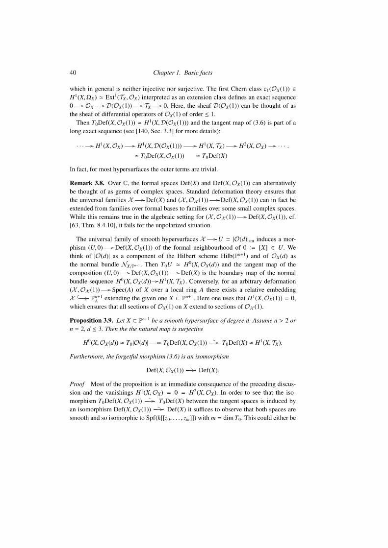
40 Chapter 1. Basic facts
which in general is neither injective nor surjective. The first Chern class c1(OX(1)) ∈H1(X,ΩX) ' Ext1(TX ,OX) interpreted as an extension class defines an exact sequence0 //OX //D(OX(1)) // TX // 0. Here, the sheaf D(OX(1)) can be thought of asthe sheaf of differential operators of OX(1) of order ≤ 1.
Then T0Def(X,OX(1)) ' H1(X,D(OX(1))) and the tangent map of (3.6) is part of along exact sequence (see [140, Sec. 3.3] for more details):
· · · // H1(X,OX) // H1(X,D(OX(1))) // H1(X, TX) // H2(X,OX) // · · · .
' T0Def(X,OX(1)) ' T0Def(X)
In fact, for most hypersurfaces the outer terms are trivial.
Remark 3.8. Over C, the formal spaces Def(X) and Def(X,OX(1)) can alternativelybe thought of as germs of complex spaces. Standard deformation theory ensures thatthe universal families X //Def(X) and (X ,OX (1)) //Def(X,OX(1)) can in fact beextended from families over formal bases to families over some small complex spaces.While this remains true in the algebraic setting for (X ,OX (1)) //Def(X,OX(1)), cf.[63, Thm. 8.4.10], it fails for the unpolarized situation.
The universal family of smooth hypersurfaces X //U = |O(d)|sm induces a mor-phism (U, 0) //Def(X,OX(1)) of the formal neighbourhood of 0 B [X] ∈ U. Wethink of |O(d)| as a component of the Hilbert scheme Hilb(Pn+1) and of OX(d) asthe normal bundle NX/Pn+1 . Then T0U ' H0(X,OX(d)) and the tangent map of thecomposition (U, 0) //Def(X,OX(1)) //Def(X) is the boundary map of the normalbundle sequence H0(X,OX(d)) //H1(X, TX) . Conversely, for an arbitrary deformation(X ,OX (1)) // Spec(A) of X over a local ring A there exists a relative embeddingX // Pn+1
A extending the given one X ⊂ Pn+1. Here one uses that H1(X,OX(1)) = 0,which ensures that all sections of OX(1) on X extend to sections of OX (1).
Proposition 3.9. Let X ⊂ Pn+1 be a smooth hypersurface of degree d. Assume n > 2 orn = 2, d ≤ 3. Then the the natural map is surjective
H0(X,OX(d)) ' T0|O(d)| // // T0Def(X,OX(1)) ∼− // T0Def(X) ' H1(X, TX).
Furthermore, the forgetful morphism (3.6) is an isomorphism
Def(X,OX(1)) ∼− // Def(X).
Proof Most of the proposition is an immediate consequence of the preceding discus-sion and the vanishings H1(X,OX) = 0 = H2(X,OX). In order to see that the iso-morphism T0Def(X,OX(1)) ∼
− // T0Def(X) between the tangent spaces is induced byan isomorphism Def(X,OX(1)) ∼
− // Def(X) it suffices to observe that both spaces aresmooth and so isomorphic to Spf(k[[z0, . . . , zm]]) with m = dim T0. This could either be

3 Automorphisms and deformations 41
deduced from the vanishing H2(X,D(OX(1))) = H2(X, TX) = 0 for n > 3 [140, Thm.3.3.11] or, simply, from the fact that |O(d)| is smooth.
Remark 3.10. The kernel of H0(X,OX(d)) // // H1(X, TX) is a quotient of H0(X, TP|X)(and in fact equals it for n ≥ 2). The latter should be thought of as the tangent spaceof the orbit through [X] ∈ |O(d)| of the natural GL(n + 2)-action on |O(d)|, see Section2.1.3.
It may be worth pointing out the following consequence, which we will only state forcubic hypersurfaces.
Corollary 3.11. Any local deformation of a smooth cubic hypersurface X ⊂ Pn+1 as avariety over k is again a cubic hypersurface.
For n = 2 it is easy to construct smooth projective deformations of cubic surfaces thatare not cubic surfaces any longer. However, for n > 2 the fact that ρ(X) = 1 allows oneto prove that global smooth projective deformations of cubic hypersurfaces are againcubic hypersurfaces, cf. [95, Thm. 3.2.5].6 The situation is more complicated when oneis interested in non-projective or, equivalently, non-Kählerian global deformations.
3.4 In [119] it has also been observed that in fact for generic hypersurfaces the auto-morphism group is trivial. Generalizations for complete intersections have been provedmore recently in [18, 34].
Theorem 3.12. Assume n > 0, d ≥ 3, and (n, d) , (1, 3). Then there exists a dense opensubset V ⊂ |O(d)|sm such that for all geometric points [X] ∈ V one has
Aut(X) = Aut(X,OX(1)) = id.
There are three proofs in the literature. The original due to Matsumura and Monsky[119] and two more recent ones by Poonen [133] and Chen, Pan, and Zhang [34]. Infact, Aut(X,OX(1)) = id also holds for (n, d) = (1, 3) as long as char(k) , 3. Forsimplicity we shall assume that (n, d) , (1, 3), (2, 4) and so Aut(X) = Aut(X,OX(1)),see Corollary 3.6.7
In [133] the result is proved by writing down an explicit equation of one smooth hy-persurface without any non-trivial polarized automorphisms. We will follow [34] adapt-ing the arguments to our situation.8 We shall begin with the following result which is ofindependent interests.
6 Thanks to J. Ottem for the reference. Compare this to the well-known fact that Def(P1 × P1) is a reducedpoint but yet P1 × P1 can be deformed to any other Hirzebruch surface Fn = P(O ⊕O(n)) with n even.
7 There is a technical subtlety for (n, d) = (2, 4) in positive characteristic which needs to be checked. Thequestion is whether for the generic quartic K3 surface all automorphisms are polarized. This is clear invanishing characteristic using transcendental techniques. In [119] the case is excluded but I believe oneshould be able to settle this one way or the other.
8 Thanks to O. Benoist for the reference.

42 Chapter 1. Basic facts
Proposition 3.13. Assume X ⊂ Pn+1, n >, is a smooth hypersurface of degree d ≥ 3over a field of characteristic zero. Then Aut(X) acts faithfully on H1(X, TX).
Proof We may assume that k algebraically closed. Suppose g ∈ Aut(X) acts triviallyon H1(X, TX). As an element g ∈ Aut(X) ⊂ PGL(n + 2) it can be lifted to an element inSL(n+2) which we shall also call g. It is still of finite order and, after a linear coordinatechange, can be assumed to act by g(xi) = λi xi for some roots of unities λi. This is whereone needs char(k) = 0.
Let F ∈ H0(P,O(d)) be a homogeneous polynomial defining X. As g(X) = X, theinduced action of g on H0(P,O(d)) satisfies g(F) = µ F for some root of unity µ. More-over, changing g by µ−1/d we may assume that µ = 1 (but possibly g is now only afinite order element in GL(n + 2)). For greater clarity, we rewrite (3.2) as the short exactsequence
W B (V ⊗ V∗)/k · id ' H0(X, TP|X) // H0(X,OX(d)) // // H1(X, TX),
with V B 〈x0, . . . , xn+1〉 and using H0(X, TX) = 0 = H1(X, TP|X) observed earlier.All maps are compatible with the action of g and, in fact, the isomorphism is GL-equivariant. Note that H0(X,OX(d)) is endowed with the action of g by interpretingOX(d) as the normal bundle NX/P. The action is compatible with the one induced by theisomorphism H0(X,OX(d)) ' H0(P,O(d))/k · F.
Thus, in order to arrive at a contradiction, it suffices to show that the g-invariant partH0(X,OX(d))g cannot map onto H1(X, TX). So it is enough to show that its dimensionh0(OX(d))g satisfies
h0(OX(d))g < h1(X, TX) + dim(Wg).
As h1(X, TX) = h0(OX(d)) − dim(W), this reduces the task to proving
dim(W) − dim(Wg) < h0(OX(d)) − h0(OX(d))g. (3.7)
Note that the left hand side equals dim(V ⊗ V∗) − dim(V ⊗ V∗)g and, as g(F) = F, theright hand side is nothing but h0(P,O(d)) − h0(P,O(d))g. The weak inequality in (3.7)follows from the obvious equality Wg = W ∩ H0(X,OX(d))g.
The strict equality follows from purely combinatorial considerations for which werefer to [34]. The idea is to write V =
⊕Vλ with Vλ B 〈xi | λi = λ〉. Then, the left
hand side is dim(W) − dim(Wg) = (n + 2)2 −∑
dim(Vλ)2. To compute the right handside, one decomposes S d(V) = S d
(⊕Vλ
)and shows that for d ≥ 3 the dimension of
the non-invariant part on the left exceeds the one on the right.9
9 This part feels a little unsatisfactory. It would be good to find a cleaner more conceptual argument forit. It is interesting to observe that the argument breaks down at this point for n = 0. And, indeed, theautomorphism group of a cubic X ⊂ P1 is never trivial.

4 Jacobian ring 43
Corollary 3.14. The group Aut(X) of a smooth hypersurface of dimension n > 0 andof degree d ≥ 3 defined over C acts faithfully on the middle cohomology Hn(X,Z).
Proof The assertion follows from the proposition by using that the contraction mapH1(X, TX) // End(Hn(X,C)) is equivariant and injective, cf. Corollary 4.22.
Proof of Theorem 3.12 As H0(X, TX) = 0, the morphism Aut //U is unramified.After passing to a dense open subset V ⊂ U, we may assume it is in fact étale. Fix[X] ∈ V and assume there exists id , g ∈ Aut(X). After base change to an openneighbourhood of [g| ∈ Aut, considered as an étale open neighbourhood of [X] ∈ V , wemay assume that there exists a relative automorphism g : X ∼
− // X , so π g = g, withg|X = g. The base change is suppressed in the notation.
The relative tangent sequence 0 // TX // TX |X // T[X]V ⊗ OX // 0 induces anexact sequence H0(X, TX |X) // T[X]V // // H1(X, TX). The surjectivity follows fromProposition 3.9. All maps are compatible with the action of g. However, as π is g-invariant, the action on T[X]V is trivial and, therefore, the action of g on H1(X, TX) istrivial as well. This contradicts Proposition 3.13.
Remark 3.15. It is worth pointing out that [133] provides equations for smooth hyper-surfaces X defined over the prime field k, so k = Fp or k = Q, such that Aut(X,OX(1)) =
id for X B X ×k k. For cubic hypersurfaces the equations are of the form c x30 +∑n
i=0 xi x2i+1 + x3
n+1, where n > 2 and char(k) , 3. The hard part of this approach is thenthe verification that the hypersurface given by this equation has no polarized automor-phisms.
Remark 3.16. Assume n ≥ 2 and d ≥ 3 as before. Then |Aut(X)| is universally bounded,i.e. there is a constant C(d, n) such that for all smooth X ∈ |O(d)|
|Aut(X)| < C(d, n).
This follows again from the fact that Aut(X /U,OX (1)) //U is a finite morphism, seeRemark 2.1.7.
The bound C(d, n) can be made effective. In [86] it has been shown that C(d, n) canbe chosen of the form C(d, n) = C(n) · dn. The bound is unlikely to be optimal. See alsoRemark 4.6.
Question 3.17. Is there anything known about the codimension of the closed set ofhypersurfaces X ∈ [O(d)| for which Aut(X,OX(1)) , id?
4 Jacobian ring
The Jacobian ring is a finite-dimensional quotient of the coordinate ring of a smoothhypersurface obtained by dividing out the partial derivatives of the defining equation.

44 Chapter 1. Basic facts
At first glance, it looks like a rather coarse invariant but it turns out to encode the iso-morphism type of the hypersurface as an abstract variety. There are purely algebraicaspects of the Jacobian ring as well as Hodge theoretic ones, which shall be explainedor at least sketched in this section.
4.1 We shall assume char(k) = 0 or, at least, that char(k) is prime to the degree d ofthe hypersurfaces under considerations and prime to d−1. The ring S B k[x0, . . . , xn+1]is naturally graded S =
⊕i≥0 S i, such that F ∈ S d for all homogeneous polynomials F
of degree d. We write ∂iF ∈ S d−1 for the partial derivatives ∂iF B ∂F/∂xi. The Hessianof F is the matrix of homogeneous polynomials of degree d − 2
H(F) B(∂2F∂xi ∂x j
)i, j.
For its determinant one has det H(F) ∈ S σ, where here and throughout we will use theshorthand
σ B (n + 2) · (d − 2). (4.1)
The reader may want to compare this number to the much larger degree of the discrim-inant divisor deg D(d, n) = (d − 1)n+1(n + 2). For the case of interest to us, d = 3, onesimply has
σ = n + 2.
Recall that the polynomial F can be recovered from its partial derivatives by means ofthe Euler equation
d · F =
n+1∑i=0
xi ∂iF. (4.2)
Definition 4.1. The Jacobian ideal of a homogeneous polynomial F ∈ S d of degree dis the homogeneous ideal
J(F) B (∂iF) ⊂ S = k[x0, . . . , xn+1]
generated by the partial derivatives of F. The Jacobian ring or Milnor ring of F is thequotient
S // // R(F) B S/J(F).
An immediate consequence of (4.2) is that the quotient map factors through the co-ordinate ring of X:
S // // S/(F) // // R(F).
If X ⊂ P B Pn+1 is the hypersurface defined by F, then we shall also write J(X)and R(X) instead of J(F) and R(F). As F is determined by X up to scaling, there is no

4 Jacobian ring 45
risk of ambiguity. If F or X are understood, we will abbreviate further to J = J(F) andR = R(F). Note that the Jacobian ring R is naturally graded.
As an immediate consequence of Lemma 3.1, one has
Corollary 4.2. For a smooth hypersurface X ⊂ P defined by a homogeneous polyno-mial F the Jacobian ring R(X) = R(F) is a zero-dimensional local ring and a finite-dimensional k-algebra.
4.2 The content of the next result is to show that the Jacobian ring R is Gorensteinwith its (one-dimensional) socle in degree σ = (n + 2) · (d − 2) and to compute thedimensions of its graded pieces.
Proposition 4.3. Assume that the homogeneous polynomial F ∈ S d defines a smoothhypersurface X ⊂ P = Pn+1. Then the Jacobian ring R B R(X) = R(F) has the followingproperties:
(i) The ring R is an Artinian graded ring with Ri = 0 for i > σ and Rσ ' k. Moreover,Rσ is generated by det H(F).
(ii) Multiplication yields a perfect pairing
Ri × Rσ−i // Rσ ' k.
(iii) The Poincaré polynomial of R is given by
P(R) Bσ∑
i=0
dimk(Ri) ti =
(1 − td−1
1 − t
)n+2
. (4.3)
For d = 3 the dimensions of the graded pieces of the Jacobian ring R(F) are simply
dimk(Ri) =
(n + 2
i
).
Proof We write fi B ∂iF. Then, by Lemma 3.1, f0, . . . , fn+1 ∈ S is a regular sequenceof homogeneous polynomials of degree d−1 and this is in fact all we need for the proof.
Let us begin by recalling basic facts about the Koszul complex of a regular sequencef0, . . . , fn+1 ∈ S . As always, Pn+1 = P(V) and so V∗ = 〈x0, . . . , xn+1〉. Then the Koszulcomplex is the complex (concentrated in (homological) degree n + 2, . . . , 0)
K•( fi) :( ∧n+2V∗ // · · · //∧kV∗ // · · · //∧2V∗ //V∗ // k
)⊗k S
with differentials
∂p(xi1 ∧ · · · ∧ xip ) =∑
(−1) j fi j · xi1 ∧ · · · ∧ xi j ∧ · · · ∧ xip .
Now, for a regular sequence ( fi) the Koszul complex is exact in degree , 0 with:
H0(K•( fi)) ' Coker (V∗ ⊗ S // S ) ' R B S/( fi),

46 Chapter 1. Basic facts
see [142]. The exactness of the complex K•( fi) // R and the fact that the differentialsin the Koszul complex are homogeneous of degree d − 1 shows
dim Ri = dim(S i) − (n + 2) dim(S i−(d−1)) ± · · ·
=
n+2∑j=0
(−1) j(n + 2
j
)dim(S i− j (d−1)).
Of course, dim(S i− j (d−1)) = h0(P,O(i − j (d − 1))) =(
n+1+i− j (d−1)i− j (d−1)
), see (1.2). This in
principle allows one to compute the right hand side. The argument can be made moreexplicit by observing that in K•( fi) only the differentials depend on the sequence ( fi).Hence, dim Ri can be computed by choosing a particular sequence, e.g. fi = xd−1
i . In thiscase, if a monomial xI = xi0
0 · · · xin+1n+1 is not contained in the Jacobian ideal ( fi = xd−1
i ),then all i j ≤ d − 2 and hence |I| ≤ (n + 2) · (d − 2) = σ. In other words, Ri = 0 for i > σ,which is not quite so obvious from the above dimension formula. Moreover, if xI < ( fi)for |I| = σ, then xI =
∏xd−2
i , i.e. Rσ is one-dimensional and generated by the Hessiandeterminant of F =
∑xd
i . To compute the Poincaré polynomial completely, observe that
R(∑
xdi
)' k[x0]/(xd−1
0 ) ⊗ · · · ⊗ k[xn+1]/(xd−1n+1)
and hence
P(R
(∑xd
i
))= P
(k[x]/(xd−1)
)n+2= (1 + t + · · · + td−2)n+2 =
(1 − td−1
1 − t
)n+2
.
One can also argue without specializing to the case of a Fermat (or any other) hyper-surface and without relying on the Koszul complex as follows. For an exact sequence0 // Mm // · · · // M0 // 0 of graded S -modules the additivity of the Poincarépolynomial implies
∑(−1) jP(M j) = 0. Now, define Ri B S/( f0, . . . , fi) and consider
the sequences 0 // Ri−1 · fi // Ri−1 // Ri // 0 . They are exact due to theregularity of the sequence ( fi). Then
P(Ri) = P(Ri−1) − td−1 · P(Ri−1) = (1 − td−1) · P(Ri−1)
and by induction
P(R) = (1 − td−1)n+2 · P(S ).
Using P(S ) = 1/(1 − t)n+2, this yields (iii) and, in particular, Ri = 0 for i > σ andRσ ' k.
Let us next show that the Hessian determinant det(∂i f j
)is not contained in the
ideal ( fi) and thus generates Rσ. For this consider the dual Koszul complex K•( fi) =
HomS (K•( fi), S ), which quite generally satisfies the duality
Hp(K•( fi)) ' Hn+2−p(K•( fi)),

4 Jacobian ring 47
see [105, Ch. 4]. So, for a regular sequence ( fi) the complex K•( fi) is exact in degree, n + 2 and Hn+2(K•) ' R. This can also be checked directly, for example by usingthat Hi(K•( fi)) ' ExtiS (R, S ). Suppose now that H =
(hi j
)is a matrix of homogeneous
polynomials of degree d− 2 such that H ·(x j
)j= ( fi)i, i.e.
∑hi j x j = fi. Then H induces
a morphism of complexes∧• H : K•( fi) // K•(xi), the dual of which is a morphism
K•(xi) // K•( fi). The latter induces in degree n + 2 the map
k ' S/(xi) ' Hn+2(K•(xi)) // Hn+2(K•( fi)) ' R, 1 // det(H),
which can also be interpreted as the map η : Extn+2S (k, S ) // Extn+2
S (R, S ) induced bythe short exact sequence 0 // (xi)/( fi) // R // k // 0. As (xi)/( fi) has zero-dimen-sional support and, thus, Extn+1
S ((xi)/( fi), S ) = 0, the map η is injective. Therefore,det(H) , 0 in R. To relate this to our assertion, observe that the Euler equation (4.2)implies H(F) ·
(x j
)j= (d − 1) (∂iF)i and set H B (1/(d − 1)) · H(F).
It remains to prove that the pairing defined by multiplication is perfect. Evidencecomes from the equation tσ · P(1/t) = P(t) for the Poincaré polynomial computedabove. This already shows that dim Ri = dim Rσ−i. Thus, to verify that the pairing isnon-degenerate, it suffices to prove that for any homogeneous g < ( fi) there exists ahomogeneous polynomial h with 0 , g · h ∈ Rσ or, equivalently, such that the degree σpart (g)σ of the homogeneous ideal (g) in R is not trivial. Let i be maximal with (g)i , 0and pick 0 , G ∈ (g)i. Suppose i < σ. Then G · (xi) ⊂ ( fi), which induces a non-trivialhomomorphism of S -modules k // R, 1 // G. Hence, dimk HomS (k,R) > 1, but thisis absurd. Indeed, splitting the Koszul complex K•( fi) into short exact sequences andusing that ExtiS (k,
∧p V∗ ⊗ S ) = 0 for i < n + 2, one finds a sequence of inclusions
HomS (k,R) // Ext1S (k,Ker(∂0))
// · · · // Extn+2
S (k,∧n+2V∗ ⊗ S ) ' k.
This concludes the proof of (ii).
Remark 4.4. Let us add a more analytic argument for the fact that the Hessian deter-minant generates the socle, cf. [70]. For this we assume k = C and define the residue ofg ∈ C[x0, . . . , xn+1] with respect to F as
Res(g) B(
12πi
)n+2 ∫Γ
g dx0 ∧ . . . ∧ dxn+1
f0 · · · · · fn+1,
where as before fi = ∂iF and Γ B x ∈ Cn+2 | | fi(x)| = εi with 0 < εi 1. Then onechecks two things:
(i) If g ∈ ( fi), then Res(g) = 0. This follows from Stokes’s theorem. Indeed, for exam-ple for g = h f0 one has
(2πi)n+2 Res(g) =
∫Γ
h dx0 ∧ . . . ∧ dxn+1
f1 · · · · · fn+1=
∫Γ0
d(
hf1 · · · fn+1
)∧dx0∧. . .∧dxn+1 = 0,

48 Chapter 1. Basic facts
as h/( f1 · · · fn+1) is holomorphic around Γ0 B z ∈ Cn+2 | | f0(z)| < ε0, | fi>0(z)| = εi.
(ii) The residue of g = det H(F) is non-zero. More precisely, Res(det H(F)) = deg( f ).Here, f : Cn+2 //Cn+2 is the map x = (xi)
// ( fi(x)), which is of degree deg( f ) =
dimOCn+2,0/( fi). Indeed,(1
2πi
)n+2 ∫Γ
det H(F) dx0 ∧ . . . ∧ dxn+1
f0 · · · · · fn+1=
(1
2πi
)n+2 ∫Γ
d f0 ∧ . . . ∧ d fn+1
f0 · · · · · fn+1
=
(1
2πi
)n+2 ∫Γ
f ∗(
dz0
z0∧ . . . ∧
dzn+1
zn+1
)= deg( f ) ·
n+1∏j=0
12πi
∫|z j |=ε j
dz j
z j
= deg( f ).
Clearly, (i) and (ii) together imply det H(F) < J(F).In [138] one finds a proof of the above proposition that reduces the assertion to state-
ments in local duality theory as in [79]. In [154] the results are deduced from globalSerre duality on Pn+1.
Here is an immediate consequence of the perfectness of the pairing Ri ×Rσ−i // Rσ.
Corollary 4.5. Assume i + j ≤ σ. Then the natural map
Ri // Hom(R j,Ri+ j)
induced by multiplication is injective.
Remark 4.6. Let X = V(F) ⊂ Pn+1 be a smooth hypersurface of degree d. Then itsgroup of polarized automorphisms Aut(X,OX(1)), which according to Corollary 3.6 isessentially always finite, acts on the finite dimensional Jacobian ring R = R(X). Theaction is graded and faithful. As a generalization of the Poincaré polynomial P(R) oneconsiders for any g ∈ Aut(X,OX(1)) the polynomial
P(R, g) B∑
tr (g |Ri) ti.
Then the Poincaré polynomial is recovered as P(R) = P(R, id). The equation (4.3) hasbeen generalized by Bott–Tate and Orlik–Solomon [129] to
P(R, g) =det (1 − g td−1 |V)
det (1 − g t |V), (4.4)
where V∗ = S 1 = 〈x0, . . . , xn+1〉. This can then be used to see that |Aut(X,OX(1))| isbounded by a function only depending on d and n, see [129, Cor. 2.7], which we havehinted at already in Remark 3.16.
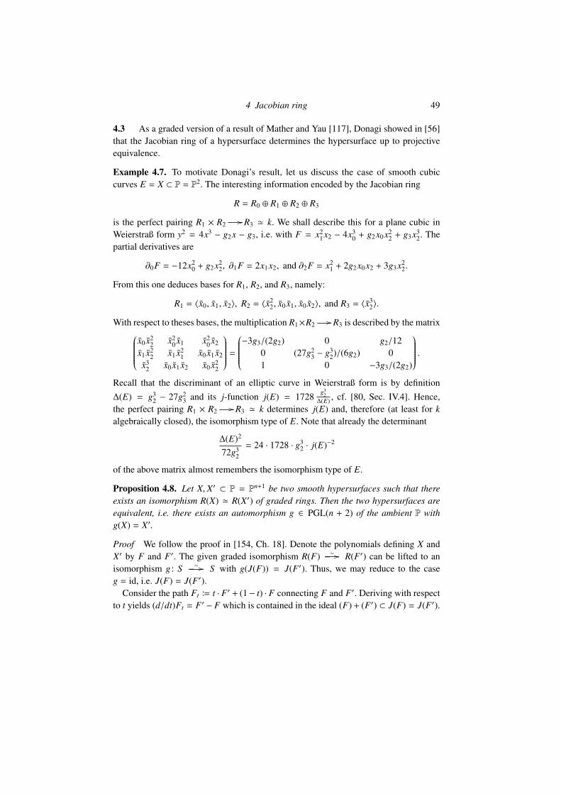
4 Jacobian ring 49
4.3 As a graded version of a result of Mather and Yau [117], Donagi showed in [56]that the Jacobian ring of a hypersurface determines the hypersurface up to projectiveequivalence.
Example 4.7. To motivate Donagi’s result, let us discuss the case of smooth cubiccurves E = X ⊂ P = P2. The interesting information encoded by the Jacobian ring
R = R0 ⊕ R1 ⊕ R2 ⊕ R3
is the perfect pairing R1 × R2 // R3 ' k. We shall describe this for a plane cubic inWeierstraß form y2 = 4x3 − g2x − g3, i.e. with F = x2
1x2 − 4x30 + g2x0x2
2 + g3x32. The
partial derivatives are
∂0F = −12x20 + g2x2
2, ∂1F = 2x1x2, and ∂2F = x21 + 2g2x0x2 + 3g3x2
2.
From this one deduces bases for R1, R2, and R3, namely:
R1 = 〈x0, x1, x2〉, R2 = 〈x22, x0 x1, x0 x2〉, and R3 = 〈x3
2〉.
With respect to theses bases, the multiplication R1×R2 // R3 is described by the matrixx0 x2
2 x20 x1 x2
0 x2
x1 x22 x1 x2
1 x0 x1 x2
x32 x0 x1 x2 x0 x2
2
=
−3g3/(2g2) 0 g2/12
0 (27g23 − g3
2)/(6g2) 01 0 −3g3/(2g2)
.Recall that the discriminant of an elliptic curve in Weierstraß form is by definition∆(E) = g3
2 − 27g23 and its j-function j(E) = 1728 g3
2∆(E) , cf. [80, Sec. IV.4]. Hence,
the perfect pairing R1 × R2 // R3 ' k determines j(E) and, therefore (at least for kalgebraically closed), the isomorphism type of E. Note that already the determinant
∆(E)2
72g32
= 24 · 1728 · g32 · j(E)−2
of the above matrix almost remembers the isomorphism type of E.
Proposition 4.8. Let X, X′ ⊂ P = Pn+1 be two smooth hypersurfaces such that thereexists an isomorphism R(X) ' R(X′) of graded rings. Then the two hypersurfaces areequivalent, i.e. there exists an automorphism g ∈ PGL(n + 2) of the ambient P withg(X) = X′.
Proof We follow the proof in [154, Ch. 18]. Denote the polynomials defining X andX′ by F and F′. The given graded isomorphism R(F) ∼
− // R(F′) can be lifted to anisomorphism g : S ∼
− // S with g(J(F)) = J(F′). Thus, we may reduce to the caseg = id, i.e. J(F) = J(F′).
Consider the path Ft B t · F′ + (1− t) · F connecting F and F′. Deriving with respectto t yields (d/dt)Ft = F′ − F which is contained in the ideal (F) + (F′) ⊂ J(F) = J(F′).

50 Chapter 1. Basic facts
On the other hand, the tangent space of the GL(n+2)-orbit at Ft is just J(Ft)d = J(F)d,which can be seen by computing for A = (ai j) ∈ M(n + 2,C)
dds
Ft ((id + s · A)x) |s=0 =∑
i
∂iFt
∑j
ai jx j.
Hence, the path Ft is tangent to all orbits and, therefore, stays inside the GL(n + 2)-orbitthrough F. This proves the assertion.
Note that in general the given isomorphism between the Jacobian rings is not inducedby any g ∈ PGL(n + 2) identifying X and X′.
Remark 4.9. There exist examples of smooth projective varieties X that can be embed-ded as hypersurfaces X
// P in non-equivalent ways. For example, the Femat quarticX ⊂ P3 is known to admit exactly three equivalence classes of degree four polarizations[49]. The three Jacobian rings are therefore non-isomorphic.
Remark 4.10. In Proposition 4.8 it is enough to assume that there is a ring isomorphismR(X) ' R(X′), not necessarily graded. Indeed, any ring isomorphism induces a gradedisomorphism
⊕mi
R/mi+1R '
⊕mi
R′/mi+1R′ , where mR ⊂ R(X) and mR′ ⊂ R(X′) are the
maximal ideals. Then use that R '⊕mi
R/mi+1R as graded k-algebras.10
4.4 For later use, we study the part of the Jacobian ring R(X) which only takes intoaccount the degrees
t(p) B (n − p + 1) · d − (n + 2).
Observe that these indices enjoy the symmetry
t(p) + t(n − p) = (n + 2) · (d − 2) = σ.
Therefore, multiplication yields perfect pairings
Rt(p) × Rt(n−p) // Rσ ' k.
Let us first check for which p one finds a non-trivial Rt(p). This is the case if and only if0 ≤ t(p) ≤ σ = (n + 2) · (d − 2), i.e. for
n + 2 − dd
≤ p ≤(n + 2) · (d − 1) − 1
d.
For d = 3 this becomesn − 1
3≤ p ≤
2n + 13
. (4.5)
Observe that t(p) = σ if and only if n − p + 1 =(n+2)·(d−1)
d , which leads to the next
Lemma 4.11. For given n and d the following conditions are equivalent:
10 Thanks to J. Rennemo for explaining this to me.

4 Jacobian ring 51
(i) d | (n + 2).(ii) There exists p ∈ Z with t(p) = 0.
(iii) There exists p ∈ Z with t(p) = σ.(iv) There exists p ∈ Z with t(p) = d.(v) There exists p ∈ Z with dim Rt(p) = 1.
(vi)⊕
Rt(p) '⊕
Rmd.
We also record that for d = 3
dimk(Rt(p)) =
(n + 2
3 (n − p + 1) − (n + 2)
)=
(n + 2
2 n + 1 − 3p
).
Exercise 4.12. Let X ⊂ Pn+1 be a smooth hypersurface of degree d. Show that∑dimk(Rt(p)) = bn(X)pr,
where bn(X)pr was computed in Section 1.3. For d = 3 this becomes the mysteriousformula ∑
p
(n + 2
2 n + 1 − 3 p
)= (−1)n · (2/3) ·
(1 + (−1)n · 2n+1
), (4.6)
cf. Remark 1.12. A geometric explanation will be given below.
4.5 There is a beautiful technique going back to [56] that, under certain numericalconditions, allows one to recover the full Jacobian ring R B R(X) from just the mu-tiplications Rd × Rt(p) // Rt(p)+d. This is useful as Rd and the Rt(p) can be describedgeometrically. We start with the geometric description of Rd(X). We recommend [38]for an instructive brief discussion and [154] for a more detailed one.
Lemma 4.13. Let X ⊂ Pn+1 be a smooth hypersurface of degree d. Assume dim(X) > 2or d ≤ 3. Then there exists a natural isomorphism
Rd(X) ' H1(X, TX).
Proof This follows from (3.2) in the proof of Corollary 3.3 and H1(X, TP|X) = 0,which holds under the present assumptions. The case n = 1, d = 3 needs an additionalargument which is left to the reader.
Example 4.14. Observe that the isomorphism confirms the dimension formula (2.2):
dim(Mn) = dim H1(X, TX) = dim R3(X) =
(n + 2
3
).
Before turning to the geometric interpretation of the spaces Rt(p)(X), we present thefollowing purely algebraic result. It was proved by Donagi [56] for generic polynomialand in [57] in general.

52 Chapter 1. Basic facts
Proposition 4.15 (Symmetrizer lemma). Assume the following conditions are satisfied:(i) i < j, (ii) i + j ≤ σ−1, and (iii) d + maxi, j ≤ σ+ 3. Then the image of the injection
R j−i // Hom(Ri,R j)
(see Corollary 4.5) is the subspace of all linear maps ϕ : Ri // R j such that for allg, h ∈ Ri one has g · ϕ(h) = h · ϕ(g) ∈ Ri+ j.
Proof The subspace described by the symmetry condition is the kernel of
Hom(Ri,R j) //Hom(∧2 Ri,Ri+ j), ϕ
// (g ∧ h // g · ϕ(h) − h · ϕ(g)).
As Ri− j obviously maps into it, one has to prove the exactness of the sequence
R j−i //Hom(Ri,R j) //Hom(∧2 Ri,Ri+ j).
This is done by comparing it to a certain Koszul complex on Pn+1. See [154, Prop. 18.21]for details.
Note that for cubic hypersurfaces the discussion below makes use of the symmetrizerlemma only for i = 1, 2, but the proof does not seem to become any easier in thesecases.
To recover large portions of R(X), the proposition is applied repeatedly. SupposeRi ×R j // Ri+ j is known. Then one recovers Ri ×R j−i // R j, for which in addition (ii)and (iii) still hold. However, it may happen that (i) no longer holds, i.e. that i ≥ j − i,but this can be remedied by swapping the factors, which does not effect the symmetryconditions (ii) and (iii). The procedure stops at some R` × R`
// R` and a moment’sthought reveals that ` = gcd(i, j). Applied to i = d and j = t(p) (or, with reversed order)this procedure eventually yields the following result.
Proposition 4.16. Assume (2n + 1)/n ≤ d. Fix p such that 0 < t(p) ≤ σ− d − 1, and let` B gcd(d, n + 2). Then multiplication
Rd × Rt(p) // Rd+t(p) = Rt(p−1)
determines the multiplication R` × R`// R2`. (Note that in general ` is not of the form
t(p).)
The next result is a special case of a more general one, which beyond the cubic caseis known for all smooth hypersurfaces except when (d, n) = (4, 4m) or d | (n + 2). Theargument is easier for cubic hypersurfaces and so we restrict to this case.
Corollary 4.17. Assume X = V(F) ⊂ Pn+1 is a smooth cubic hypersurface of dimensionn > 2 with 3 - (n + 2). Then there exist integers p with 0 < t(p) ≤ n − 2 and for eachof them the graded algebra R = R(X), and hence by Proposition 4.8 also X, is uniquelydetermined by the multiplication R3 × Rt(p) // R3+t(p).

4 Jacobian ring 53
Proof The condition 0 < t(p) ≤ σ − d − 1 in Proposition 4.16 turns for d = 3 into (cf.(4.5))
n + 3 ≤ 3p < 2n + 1, (4.7)
which has integral solutions for all n > 2. For any such p, multiplication R3(X) ×Rt(p) // R3+t(p) determines R1 × R1 // R2, as 3 - (n + 2) implies gcd(3, t(p)) = 1.
Suppose this multiplication is isomorphic to another one R′1 × R′1 // R′2 associatedwith a cubic X′ = V(F′) ⊂ Pn+1. The isomorphism R1 ' R′1 corresponds to a linearcoordinate change g : 〈x0, . . . , xn+1〉
∼− // 〈x0, . . . , xn+1〉 and the compatibility with the
multiplication can be interpreted as an isomorphism(k[x0, . . . , xn+1]2 ' S 2(R1) // R2
)'
(k[x0, . . . , xn+1]2 ' S 2(R′1) // R′2
).
Hence, under g, their kernels are identified, which are spanned by the partial derivatives∂iF and ∂iF′, respectively. Thus, g induces a ring isomorphism k[x0, . . . , xn+1] ∼
− //
k[x0, . . . , xn+1] that restricts to J(X) ∼− // J(X′) and, hence, R(X) ' R(X′).
Note that under the assumptions of Corollary 4.17, there always exists p with t(p) = 1or t(p) = 2. The result covers, for example, cubics of dimension n = 2, 3, 5, 6, 8, 9, forwhich we list the admissible t(p):
n 0 < t(p) ≤ σ − 4 = n − 2
3 t(2) = 15 t(2) = 5, t(3) = 26 t(3) = 4, t(4) = 18 t(3) = 8, t(4) = 5, t(5) = 29 t(4) = 7, t(5) = 4, t(6) = 1
Remark 4.18. The result is sharp. For example, for n = 4, the only 0 ≤ t(p) ≤ σ = 6are t(1) = 6, t(2) = 3, and t(3) = 0. But the pairing R3 × R3 // R6 ' k does certainlynot determine the cubic nor does the identity R3 × R0 // R3.
4.6 The next step is to describe the parts Rt(p)(X) geometrically. This is the followingcelebrated result due to Carlson and Griffiths [30].
Theorem 4.19 (Carlson–Griffiths). Let X ⊂ Pn+1 be a smooth hypersurface of degreed. Assume n > 2 or d ≤ 3. Then for all integers p there exists an isomorphism
Hp,n−p(X)pr ' Rt(p)(X), (4.8)
with t(p) = (n − p + 1) · d − (n + 2), compatible with the natural pairings on both sides,

54 Chapter 1. Basic facts
i.e. there exist commutative diagrams
Hp,n−p(X)pr × Hn−p,p(X)pr
'
'
// Hn,n(X)pr
'
Rt(p)(X) × Rt(n−p)(X) // Rσ(X).
(4.9)
Moreover, using the isomorphism H1(X, TX) ' Rd(X), cf. Lemma 4.13, and the pairingTX ×Ω
pX
//Ωp−1X , one obtains commutative diagrams
H1(X, TX) × Hp,n−p(X)pr
'
'
// Hp−1,n−p+1(X)pr
'
Rd(X) × Rt(p)(X) // Rt(p−1)(X),
(4.10)
The proof of the theorem is involved and we will not attempt to present it in full.However, we will outline the most important parts of the general theory that enter theproof and, in particular, explain how to establish a link between the Jacobian ring andthe primitive cohomology at all. As we will restrict to the case of hypersurfaces in Pn+1
throughout, certain aspects simplify. We refer to [29] and [154] for more details andsome of the crucial computations.
(i) The de Rham complex of a (smooth) k-variety X of dimension n is the complex
Ω•X : OX //ΩX //Ω2X
// · · · //ΩnX .
The ΩiX B
∧i ΩX are coherent sheaves (here in the Zariski topology), but the differen-tials d : Ωi
X//Ωi+1
X are only k-linear. The de Rham cohomology of X is then defined asthe hypercohomology of this complex:
H∗dR(X/k) B H∗(X,Ω•X),
which can be computed via the Hodge–de Rham spectral sequence
Ep,q1 = Hq(X,Ωp
X) +3 Hp+qdR (X/k). (4.11)
Note that the E1-terms are just cohomology groups of coherent sheaves. The spectralsequence is associated with the Hodge filtration, which is induced by the complexes
F pΩ•X : ΩpX
// · · · //ΩnX
concentrated in degrees p, . . . , n and the natural morphism F pΩ•X//Ω•X . Then one
defines
F pH∗dR(X/k) B Im(H∗(F pΩ•X) //H∗(Ω•X) = H∗dR(X/k)
).

4 Jacobian ring 55
Remark 4.20. If X is smooth and projective over a field k satisfying char(k) = 0 orchar(k) = p > dim(X) and X is liftable to W2(k), then (4.11) degenerates [51]. This ap-plies to smooth hypersurfaces X ⊂ Pn+1, for which the assumption on the characteristicof k can be avoided, cf. Section 1.6.
(ii) For open varieties the Hodge–de Rham spectral sequence does not necessarilydegenerate, but a replacement is available. Consider the open complement j : U B P \X // P = Pn+1 of a smooth hypersurface X ⊂ P. There are quasi-isomorphisms (see
the discussion following (4.18))
Ω•P(log(X)) ∼− // Ω•P(∗X) = j∗Ω•U . (4.12)
Here, ΩpP(∗X) B j∗Ω
pU (in the Zariski topology!) is the sheaf of meromorphic p-forms
on P with poles (of arbitrary order) along X. Furthermore, Ω1P(log(X)) ⊂ Ω1
P(∗X) isdefined as the subsheaf locally generated by d log( f ) =
d ff , where f is the local equation
for X, and ΩpP(log(X)) B
∧p(Ω1
X(log(X))). In our case, X = V(F) and
Ω1P(log(X))|U j = d log(F j)OU j =
dF j
F jOU j
on the standard open subset U j B P \ V(x j) with F j B F(x0/x j, . . . , xn+1/x j). Thedifferentials in both complexes are the usual ones. By construction, Ω•P(log(X)) is thesubcomplex of forms α with α and dα having at most simple poles along X. The Hodgefiltration in the open case is defined by
F pΩ•P(log(X)) : ΩpP(log(X)) // · · · //Ωn+1
P (log(X))
(and not as the direct image of F pΩ•U) in degrees p, . . . , n + 1. It induces the spectralsequence
Ep,q1 = Hq(P,Ωp
P(log(X))) +3 Hp+q(P,Ω•P(log(X))), (4.13)
where the right hand side is isomorphic to
H•(P,Ω•P(log(X))) ' H∗(P,Ω•P(∗X)) ' H∗dR(U/k).
Again due to [51], this spectral sequence degenerates under the assumptions of Remark4.20 and so in particular for smooth hypersurfaces.
Observe that the residue
res :d ff
h // h|X
yields a short exact sequence 0 //Ω1P
//Ω1P(log(X)) // i∗OX // 0. Taking exterior
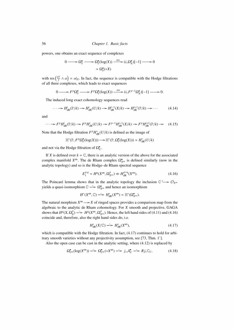
56 Chapter 1. Basic facts
powers, one obtains an exact sequence of complexes
0 // Ω•P// Ω•P(log(X)) res // (i∗Ω•X)[−1] // 0
' Ω•P(∗X)
with res(
d ff ∧ α
)= α|X . In fact, the sequence is compatible with the Hodge filtrations
of all three complexes, which leads to exact sequences
0 // F pΩ•P// F pΩ•P(log(X)) res // (i∗F p−1Ω•X)[−1] // 0.
The induced long exact cohomology sequences read
· · · // HidR(P/k) // Hi
dR(U/k) // Hi−1dR (X/k) // Hi+1
dR (P/k) // · · · (4.14)
and
· · · // F pHidR(P/k) // F pHi
dR(U/k) // F p−1Hi−1dR (X/k) // F pHi+1
dR (P/k) // (4.15)
Note that the Hodge filtration F pH∗dR(U/k) is defined as the image of
H∗(P, F pΩ•P(log(X))) //H∗(P,Ω•P(log(X))) ' H∗dR(U/k)
and not via the Hodge filtration of Ω•U .
If X is defined over k = C, there is an analytic version of the above for the associatedcomplex manifold Xan. The de Rham complex Ω•Xan is defined similarly (now in theanalytic topology) and so is the Hodge–de Rham spectral sequence
Ep,q1 = Hq(Xan,Ω
pXan ) +3 Hp+q
dR (Xan). (4.16)
The Poincaré lemma shows that in the analytic topology the inclusion C // OXan
yields a quasi-isomorphism C ∼− // Ω•Xan and hence an isomorphism
H∗(Xan,C) ∼− // H∗dR(Xan) = H∗(Ω•Xan ).
The natural morphism Xan // X of ringed spaces provides a comparison map from thealgebraic to the analytic de Rham cohomology. For X smooth and projective, GAGAshows that Hq(X,Ωp
X) ∼− // Hq(Xan,Ω
pXan ). Hence, the left hand sides of (4.11) and (4.16)
coincide and, therefore, also the right hand sides do, i.e.
H∗dR(X/C) ∼− // H∗dR(Xan), (4.17)
which is compatible with the Hodge filtration. In fact, (4.17) continues to hold for arbi-trary smooth varieties without any projectivity assumption, see [73, Thm. 1’].
Also the open case can be cast in the analytic setting, where (4.12) is replaced by
Ω•Pan (log(Xan)) ∼− // Ω•Pan (∗Xan) ∼
− // j∗A•U∼− // R j∗CU . (4.18)

4 Jacobian ring 57
Here, the complex AU is the standard C∞-de Rham complex.The verification of the quasi-isomorphisms in (4.18), and, similarly, in (4.12), is read-
ily reduced to the case of U = C \ 0 // C. In this case,
Ω•C(log(0))(C) : OC // dzz OC,
Ω•C(∗0)(C) :∑
zn OC // ∑ zndzOC,
j∗A•(C) : C∞U // dx C∞U + dy C∞U // (dx ∧ dy) C∞U .
The cohomology of all three satisfies Hi ' C for i = 0, 1 and Hi = 0 otherwise.Also, there is an analytic version of (4.13) and there exists a natural isomorphism
H∗(P,Ω•P(log(X))) ' H∗(Pan,Ω•Pan (log(Xan))).
To simplify the notation, we will from now on also write X, U, and P for the asso-ciated analytic varieties. Then the exact sequence (4.14) becomes the classical Gysinsequence
· · · // Hi(P,C) // Hi(U,C) // Hi−1(X,C) // Hi+1(P,C) // · · · .
This is interesting only for i − 1 = n. As the map Hk(X,C) // Hk+2(P,C) is surjectivefor k = n − 1, n, one finds
Hn+1(U,C) ∼ // Hn(X,C)pr
F pHn+1(U,C)
⋃∼ // F p−1Hn(X,C)pr.
⋃
However, as it turns out, the Hodge filtration is difficult to compute and it is prefer-able to replace it by the pole filtration F•pol of the complex Ω•P(∗X). Under the quasi-isomorphisms (4.12) and (4.18) the two compare as follows
F pΩ•P(log(X))⋂ : ΩpP(log(X))⋂ // Ωp+1
P (log(X))⋂ · · · // Ωn+1P (log(X))⋂
F ppolΩ
•P(∗X) : Ω
pP(X) // Ωp+1
P (2X) · · · // Ωn+1P ((n − p + 2)X).
This is usually not a quasi-isomorphism. However, using that H∗(P,C)pr = 0 and apply-ing Bott vanishing, see Section 1.2, one finds
F ppolH
n+1(U,C) ' F pHn+1(U,C).
The advantage of using the pole filtration comes from the following
Lemma 4.21 (Griffiths). Let X ⊂ P = Pn+1 be a smooth hypersurface.

58 Chapter 1. Basic facts
Then F p+1Hn+1(U,C) ' F pHn(X,C)pr is isomorphic to
F p+1pol Hn+1(U,C) '
H0(P,Ωn+1P ((n − p + 1)X))
dH0(P,ΩnP((n − p)X))
(4.19)
and F p+1Hn+1(U,C)/F p+2Hn+1(U,C) ' Hp,n−p(X)pr is isomorphic to
F p+1pol Hn+1(U,C)
F p+2pol Hn+1(U,C)
'H0(P,Ωn+1
P ((n − p + 1)X))
H0(P,Ωn+1P ((n − p)X)) + dH0(P,Ωn
P((n − p)X)). (4.20)
Proof By definition, the left hand side in (4.19) is the image of the map
Hn+1(P, F p+1pol Ω•P(∗X)) //Hn+1(P,Ω•P(∗X)).
The natural map Ωn+1P ((n − p + 1)X)[−(n + 1)] // F p+1
pol Ω•P(∗X) induces
H0(P,Ωn+1P ((n − p + 1)X)) // F p+1
pol Hn+1(P,Ω•P(∗X)) ' F p+1
pol Hn+1(U,C).
It is rather straightforward to show that the map is surjective and that its kernel is theimage of d : H0(P,Ωn
P((n − p)X)) // H0(P,Ωn+1P ((n − p + 1)X)). The isomorphism in
(4.20) follows.
Observe that
H0(P,Ωn+1P ((n − p + 1)X)) ' H0(P,O((n − p + 1) · d − (n + 2)))
' H0(P,O(t(p))).
Thus, in order to prove (4.8), it suffices to show that the image of
(∂iF) : H0(P,O((n − p) · d − (n + 2))) // H0(P,O(t(p)))
equals H0(P,Ωn+1P ((n − p)X)) + dH0(P,Ωn
P((n − p)X)). This is a rather unpleasant com-putation in terms of rational differential forms on P and Cn+2. We omit this here andrefer to [154, Thm. 18.10] or [29, Ch. 3.2].11
To prove the commutativity of (4.9) one first needs to fix an appropriate isomorphismHn,n(X)pr ' Rσ(X) which again involves rational forms. Also the commutativity of(4.10) is not straightforward. One has to argue that multiplication
H0(P,O(d)) × H0(P,O(t(p))) // H0(P,O(t(p − 1)))
11 One could try an alternative argument: Apply∧n+1 to the Euler sequence to obtain 0 //O(−(n +
2)) //O(−(n + 1))⊕n+2 // ΩnP
// 0. Tensor with O((n − p) · d) and consider the composition
H0 (P,O((n − p) · d − (n + 1)))⊕n+2 // // H0(P,ΩnP((n− p) ·d)) d // H0(P,Ωn+1
P ((n− p + 1) ·d)), whichshould be compared to the map given by (∂iF). But the attempt becomes quickly as technical as the stan-dard approach.

5 Quadric fibrations and ramified covers 59
is related to the contraction
H1(X, TX) × Hn−p(X,ΩpX) // Hn−p+1(X,Ωp−1
X )
via the surjection H0(P,O(d)) // H0(X,OX(d)) // H1(X, TX). The multiplication takesplace in the top degree n + 1 of F p+1
pol Ω•P(∗X), whereas the contraction applies to the low-est degree (from degree p to p − 1).
We conclude this section by a result that will later be used to prove that the periodmap is unramified. We state the result for cubic hypersurfaces only.
Corollary 4.22 (Infinitesimal Torelli Theorem). Let X ⊂ Pn+1 be a smooth cubic hyper-surface of dimension n > 2. Then the contraction TX ×Ω
pX
//Ωp−1X yields an injection
H1(X, TX) // Hom
⊕p+q=n
Hp,q(X)pr,⊕p+q=n
Hp−1,q+1(X)pr
Proof There exists a p such that 0 ≤ t(p) ≤ σ−3. Then by Corollary 4.5 multiplicationin the Jacobian ring R(X) yields an injection
R3 // Hom(Rt(p),Rt(p)+3).
Now use Rt(p) ' Hp,n−p(X)pr and the compatibility of the multiplication in R(X) withthe contraction map.
5 Quadric fibrations and ramified covers
This part is devoted to standard constructions for cubic hypersurfaces, for example usinglinear projection to view them as quadratic fibrations or studying triple cover of theambient projective space ramified along the cubic.
5.1 Let P B P(W) ⊂ P B P(V) be a linear subspace. Here, dim(V) = n + 2 andk = dim(W). Furthermore, pick a generic linear subspace P(U) ⊂ P(V) of codimensionk. Here, generic means that the composition U ⊂ V // // V/W is an isomorphism or,equivalently, that U + W = V .
The linear projection : P // P(U) ' P(V/W) from P is the rational map that
sends x ∈ P \ P to the unique point of intersection of the linear subspace x P ' Pk
with P(U) ' Pn+1−k. It is the rational map associated with the linear system |IP ⊗
O(1)| ⊂ |O(1)| with base locus P ⊂ P, which is resolved by a simple blow-up. Theresulting morphism ϕ : BlP(P) // P(V/W) is associated with the complete linear sys-

60 Chapter 1. Basic facts
tem |τ∗O(1) ⊗O(−E)|:
E = P(NP/P)
// BlP(P)
τ
ϕ
%%P // P // P(V/W).
The fibre ϕ−1(y), y ∈ P(U) ' P(V/W), is the strict transform of Pk ' y P ⊂ P inBlP(P). So, all fibres of ϕ : BlP(P) // P(V/W) are projective spaces Pk and, indeed,BlP(P) ' P(F ∗) for the locally free sheaf F B ϕ∗τ
∗O(1) on P(V/W) which is of rankk +1. To determine F explicitly, tensor the structure sequence of the exceptional divisorE ⊂ BlP(P) with τ∗O(1) to get the short exact sequence
0 // τ∗O(1) ⊗O(−E) // τ∗O(1) // τ∗O(1)|E // 0
' ϕ∗O(1) ' Oϕ(1) ' O(1, 0)
(5.1)
Here, we use that NP/P ' V/W ⊗O(1), which yields an isomorphism
E = P(NP/P) ' P × P(V/W)
compatible with the two natural projections. This also shows that O(E)|E ' O(1,−1) onE ' P×P(V/W). In particular, ϕ∗O(1)|E ' (τ∗O(1)⊗O(−E))|E ' O(0, 1). Therefore, ϕrestricted to E is the projection onto P(V/W). Thus, F is described by the direct imageunder ϕ of (5.1)
0 // O(1) // F // H0(P,O(1)) ⊗OP(V/W) // 0.
The sequence splits, which yields a non-canonical isomorphism F ' O(1) ⊕ (W∗ ⊗OP(V/W)) and, hence, det(F) ' O(1), which is all we shall use.
Let now X ⊂ P = P(V) be a cubic hypersurface with equation F ∈ H0(P,O(3)). Thepull-back τ∗F is a section of τ∗O(3), whose zero divisor V(τ∗F) is the total transformof X. If P ⊂ P is contained in X (cf. Exercise 3.2.4), then the total transform has twocomponents, E and the strict transform BlP(X) of X ⊂ P. More precisely, in this case F iscontained in H0(P,O(3)⊗IP) ⊂ H0(P,O(3)) and τ∗F in H0(BlP(P), τ∗O(3)⊗O(−E)) ⊂H0(BlP(P), τ∗O(3)). Therefore,
BlP(X) = V(τ∗F) ∈ |τ∗O(3) ⊗O(−E)|
in BlP(P). To describe BlP(X) as a quadric fibration over P(V/W), we compute the directimage of τ∗F under ϕ. First, observe that
τ∗O(3) ⊗O(−E) ' τ∗O(2) ⊗ (τ∗O(1) ⊗O(−E)) ' Oϕ(2) ⊗ ϕ∗O(1).
Hence,
ϕ∗(τ∗O(3) ⊗O(−E)) ' ϕ∗(Oϕ(2) ⊗ ϕ∗O(1)) ' S 2(F) ⊗O(1)

5 Quadric fibrations and ramified covers 61
and, therefore, τ∗F can be thought of as a section q ∈ H0(P(V/W), S 2(F) ⊗O(1)) or asa homomorphism q : F ∗ //F ⊗O(1). Then the fibre of BlP(X) ⊂ BlP(P) ' P(F ∗) overt ∈ P(V/W) is the quadric defined by q ∈ S 2(F(t)). In particular, the fibre is smoothif and only if this quadric is non-degenerate. Hence, the discriminant divisor DP ofϕ : BlP(X) // P(V/W) is
DP = V(det(q)) ⊂ P(V/W).
Here, det(q) : det(F)∗ // det(F)⊗O(k+1) is viewed as a section of det(F)2⊗O(k+1) 'O(k + 3). The discussion is summarized by the following classicial fact, see e.g. [22,Lem. 2] for n = 3 and [9, Ch. 4].
Proposition 5.1. Assume a smooth cubic hypersurface X ⊂ Pn+1 contains a linearsubspace P = Pk−1. Then the linear projection from P defines a morphism
ϕ : BlP(X) // // Pn+1−k (5.2)
with a quadric hypersurface in y P ' Pk as the fibre over y. The fibres are singularexactly over the discriminant divisor DP ∈ |O(k + 3)|.
We are most interested in the case k = n − 1.
Corollary 5.2. Assume X ⊂ Pn+1 is a smooth cubic hypersurface containing a linearP = Pn−2 ⊂ X ⊂ Pn+1. Linear projection from P yields a quadric fibration BlP(X) // P2
with discriminant curve DP ∈ |O(n + 2)|.
Remark 5.3. Assume Pn−2 ' P ⊂ X ⊂ P = Pn+1 are as above. The quadratic fibrationBlP(X) // P2 allows one to prove the unirationality (of degree two) of X, cf. Corollary3.1.15. Indeed, pick a generic P3 ⊂ P and let S be the intersection of τ−1(P3) ⊂ BlP(P),which is the blow-up of P3 in the point of intersection x of P3 and P, and BlP(X) ⊂BlP(P). Clearly, S is the blow-up of the cubic hypersurface S : X ∩ P3 in x. The genericfibre of ϕ : S // P2 over y ∈ P2 is the intersection of the quadric ϕ−1(y) ⊂ y P with theline P1 ' P3 ∩ y P and, therefore, consists of two points, i.e. S // P2 is of degree two.The base change BlP(X) ×P2 S // P2 is a quadric fibration with a section and hencerational.
In fact, for n ≥ 7 the existence of Pn−2 ⊂ X implies the rationality of X, see [9, Cor.4.2]. Indeed, the scheme theoretic generic fibre is a quadric over the C2-field K(P2) =
K(S ), cf. [106].
If the existence of a complementary linear space contained in the cubic hypersurfaceX is assumed, not only unirationality but in fact rationality of X can be proved.
Corollary 5.4. Assume that a smooth cubic hypersurface X ⊂ Pn+1 contains Pk−1 '
P(W) ⊂ X and a complementary Pn+1−k ' P(W ′) ⊂ X, i.e. such that W + W ′ = V or,

62 Chapter 1. Basic facts
equivalently, P(W) ∩ P(W ′) = ∅. Then the quadric fibration (5.2) admits a section. Inparticular, X is rational.
Proof The section is of course given by the inclusion Pn+1−k ⊂ X. As any quadric ad-mitting a rational point is rational, the scheme-theoretic generic fibre ϕ−1(η) is a rationalquadric over K(Pn+1−k). Hence, BlP(X) is rational and, therefore, X it self is.
Example 5.5. In fact, assuming the existence two complementary linear subspacesP(W),P(W ′) ⊂ X, i.e. such that W ⊕ W ′ = kn+2, the rationality of X can also be de-duced from the following construction. Consider the rational map
ψ : P(W) × P(W ′) // // X
that sends a pair (x, x′) to the residual point of intersection of x, x′ ⊂ xx′ ∩ X. This iswell defined for all (x, x′) such that the line xx′ is not contained in X, which describes anon-empty open subset of P(W)×P(W ′). As any point z ∈ X\(P(W)∪P(W ′)) is containedin a unique line intersecting both spaces, P(W) and P(W ′), the map ψ is genericallyinjective and, therefore, X is rational.
Typical examples include even-dimensional cubics X ⊂ Pn+1, n = 2m, containingtwo disjoint linear subspaces Pm ⊂ X. In this case, the construction yields a rationalparametrization Pm × Pm // // X ⊂ P2m+1 .
Rationality of X, for example in dimension four, can also be deduced from the exis-tence of other types of surfaces. We recommend [83] for further information.
5.2 The generic hyperplane section of a smooth cubic hypersurface yields again asmooth cubic hypersurface of one less dimension. In Section ??.?? we shall discuss howmany hypersurfaces can be obtained as hyperplane sections of a fixed hypersurfaces.But the procedure can also be reversed. There is an almost canonical way of associatingwith a smooth cubic hypersurface X ⊂ Pn+1 a smooth cubic hypersurface X ⊂ Pn+2. Infact, the construction works for hypersurfaces of any degree d.
Let X = V(F) ⊂ Pn+1 be any hypersurface of degree d given by a polynomial F =
F(x0, . . . , xn+1) ∈ H0(Pn+1,O(d)). Then F B F − xdn+2 ∈ H0(Pn+2,O(d)) describes a
hypersurface X B V(F) ⊂ Pn+2. Clearly, X is a hyperplane section of X, namely
X = X ∩ V(xn+2).
Observe that X is smooth if and only if X is smooth.Note that X ⊂ Pn+1 determines its defining equation F only up to a scaling factor, i.e.
V(F) = V(λ F) for all λ ∈ k∗, and this does effect the equation F. However, at least if kcontains dth roots, the two hypersurfaces V(F − xd
n+2) and V(λ F − xdn+2) only differ by
a linear coordinate change [x0 : · · · : xn+1 : xn+2] // [x0 : · · · : xn+1 : λ1/d xn+2].It turns out that X is not only a hyperplane section of X. The rational map given by the

5 Quadric fibrations and ramified covers 63
projection Pn+2 // Pn+1 that drops the last coordinate is regular along X ⊂ Pn+2. Itdefines a finite morphism, and in fact a cyclic cover, of degree d
π : X // // Pn+1
branched over X ⊂ Pn+1. More precisely, π−1(X) = d X as divisors in X and
π : X = X ∩ V(xn+2) ∼− // X.
This basic construction has been successfully used to relate moduli spaces of cubichypersurfaces of different dimensions. We shall come back to this in Section ??.??.
5.3

2
Moduli spaces
1 GIT-quotient
To study the geometry of a particular hypersurface X ⊂ P = Pn+1 or to understandhow a certain feature changes when X is deformed, the actual embedding of X into theprojective space P is often of no importance. The embeddings of a fixed X into P areparametrized by the choice of a basis of H0(X,OX(1)) up to scaling.1 So, instead of thelinear system |OP(d)| one is really interested in the quotient |OP(d)|/GL(n + 2). Ideally,one would like this quotient to exist in the category of varieties or schemes and to comewith a universal family. However, as it turns out, this is too much to ask for.
Example 1.1. Consider the easiest case of interest to us: d = 3 and n = 0, i.e.three points in P1. Up to a linear coordinate change, there are only three possibilities:x1, x2, x3 (three distinct points), 2 · x1, x2 (two distinct points of which one withmultiplicity two), or 3x (a triple point). Thus, the moduli space parametrizing all hy-persurfaces X ⊂ P1 of degree three should consists of three points. On the other hand,together with all possible embeddings they are parametrized by the projective space|OP1 (3)|, which is connected and, therefore, does not admit a morphism onto a discon-nected space.
The same phenomenon can be described in terms of orbit closures. For example, thelimit of the one-parameter subgroup diag(t, 1/t) applied to the set V(x2
0 x1 − x0 x21) =
0,∞, [1 : 1] viewed as a point in |OP1 (3)| is 2 ·0,∞ for t //∞ and 0, 2 ·∞ for t //0.Hence, all these points should be identified under the quotient map to any moduli spacewith a reasonable geometric structure.
Similar phenomena occur in higher dimensions and for all d > 1. The way out isto only allow stable hypersurfaces. They are parametrized by an open subset of |OP(d)|
Version Aug 02, 2018.1 For n ≥ 2 and d , n + 2 the line bundle OX(1) itself does not depend on the embedding, as it is determined
by the property that OX(d − (n + 2)) ' ωX . For n > 2 one can alternatively use that OX(1) is the amplegenerator of Pic(X).
64

1 GIT-quotient 65
and include all smooth hypersurfaces. This then leads to a quasi-projective moduli space(without universal family in general) parametrizing orbits of hypersurfaces. To obtaina projective moduli space one has to allow semi-stable hypersurfaces which, however,leads to a moduli space that identifies certain orbits.
We briefly review the main features of GIT needed to understand moduli spaces of(smooth, cubic) hypersurfaces. We recommend [111, Ch. 6] for a quick introduction andthe classic [124] or the textbooks [54, 121] for more details and references. Althoughwe definitely want the moduli spaces to be defined over arbitrary fields, we shall assumethat k is algebraically closed, just to keep the discussion geometric.
1.1 Let A be a finite type (say integral) k-algebra and G a linear algebraic groupover k with an action on X = Spec(A) or, equivalently, an action on A. If a quotientX // X/G in the geometric sense exists, then X/G = Spec(AG), where AG ⊂ A is theinvariant ring. In order for X/G to be a variety, the ring AG would need to be again offinite type. This is Hilbert’s 14th problem which has been answered by Hilbert himselfin characteristic zero for G = SL and in general by Nagata and Harboush, see [124] orthe entertaining [123] for a historic account, references, and proofs:
If G is reductive, then AG is again a finite type k-algebra.
This seems to settle the question in the affine case by just defining X/G B Spec(AG)with the quotient morphism X // X/G induced by the inclusion AG ⊂ A. However, thisis, in general, a quotient only in a weaker sense.
Definition 1.2. A morphism π : X // Y is a categorical quotient for the action of agroup G on X if it is G-invariant2 and if any other G-invariant morphism π′ : X // Y ′
factors uniquely through a morphism Y // Y ′.A G-invariant morphism π : X // Y is a good quotient if it satisfies the following
conditions: (i) π is affine and surjective; (ii) π(Z) of any closed G-invariant subset Z ⊂ Xis closed; (iii) π(Z1) ∩ π(Z2) = π(Z1 ∩ Z2) for all closed G-invariant sets Z1,Z2 ⊂ X; and(iv) OY is the sheaf of G-invariant sections of OX , i.e. OY ' (π∗OX)G which means thatπ∗ : OY (U) ∼
− // OX(π−1(U))G for all open U ⊂ Y .A good quotient is geometric if in addition the pre-image of any closed point is an
orbit.3
By definition, any geometric quotient is a good quotient and, as proved in [124], anygood quotient is also a categorical quotient:
geometric ⇒ good ⇒ categorical.
2 i.e. the two morphisms G × X // X defined by the second projection and by the group action composedwith π coincide
3 The exact definition of these notions varies from source to source. The subtle differences will be of noimportance in our situation.

66 Chapter 2. Moduli spaces
Note that a good quotient is equipped with the quotient topology and parametrizes theclosed orbit of the action. Hence, a good quotient is geometric exactly when all orbitsare closed, see [111, Prop. 6.1.7].
The main results on affine quotients is the following, cf. [124] or [111, Prop. 6.3.1]:
If a reductive linear algebraic group G acts on an affine variety X = Spec(A), i.e. A is afinite type k-algebra, then X // X//G B Spec(AG) is a good quotient.
In particular, it is a categorical quotient, but usually not a geometric one.
1.2 With certain modifications, the same recipe can be applied to projective varieties.Assume A =
⊕i≥0 Ai is a finite type graded k-algebra generated by A1 and assume that
the projective variety X = Proj(A) is endowed with the action of a reductive linear alge-braic group. Note that, in contrast to the affine case, the action is not necessarily inducedby an action of G on A. However, we shall assume it is, in which case it is induced bya G-action on A1. This is called a linearization. Geometrically it is realized by an em-bedding X
// Proj(S ∗(A1)) ' Pm such that the action of G on X is the restriction ofan action of G on Pm induced by a linear representation G //GL(A1).
One is tempted to imitate the affine case and define the quotient simply as Proj(AG).Note that AG is naturally graded and again of finite type, but possibly not generated indegree one. This can be easily remedied by passing to
⊕i≥0 Ami for some m > 0. How-
ever, the graded inclusion AG ⊂ A does not define a morphism between the associatedprojective schemes. Indeed, a homogeneous prime or maximal ideal in A may intersectAG in its inessential ideal (AG)+ =
⊕i>0(AG)i. In other words, there exists a morphism
Xss // Xss//G B Proj(AG)
only on the open set Xss B X \ V((AG)+) ⊂ X. This naturally leads to the centraldefinition in GIT.
Definition 1.3. A point x ∈ X is semi-stable if it is contained in the open subset Xss ⊂ X,i.e. if there exists a homogeneous G-invariant f ∈ Ai, for some i > 0, with f (x) , 0. Apoint x ∈ X is stable if x is semi-stable and the induced morphism G // Xss is proper,i.e. the orbit G · x is closed in Xss and the stabilizer Gx is finite.
Exercise 1.4. For a linearized action of a reductive group G on P(V), a point [x] ∈ P(V)is semi-stable if and only if 0 < G · x ⊂ V . A point [x] ∈ P(V) is stable if and only if themorphism G // V , g // g · x is proper.
Using open affine covers, the problem is reduced to the affine case which eventuallyleads to the following key result in GIT.
Theorem 1.5 (Mumford). Assume that a linearization of the action of a reductive lin-ear algebraic group G on X = Proj(A) has been fixed. Then the natural morphismXss // Xss//G is a good quotient.

1 GIT-quotient 67
1.3 Let us turn to the concrete GIT problem that concerns us. Consider G B SL(n+2)with its natural action on Pn+1 and the induced action on all complete linear systems|O(d)|. Instead of SL(n + 2) one often considers PGL(n + 2). Both groups are reductiveand the orbits of their actions on |O(d)| are of course the same. The advantage of work-ing with SL is that its action on |O(d)| comes with a natural linearization. The relevantresult for us is the following, see [98, Sec. 11.8] for the arithmetic version over Spec(Z).
Corollary 1.6. Every smooth hypersurface X ⊂ P of degree d ≥ 3 defines a stable point[X] ∈ |O(d)| for the action of G = SL(n + 2), i.e.
U(d, n) = |O(d)|sm ⊂ |O(d)|s.
Proof The semi-stability is an immediate consequence of Theorem 1.2.2 and holds infact for d > 1. Indeed, the complement of U(d, n) ⊂ PN = |O(d)| is the discriminant divi-sor D = D(d, n), which is the zero set V(∆) of the discriminant ∆ = ∆d,n ∈ H0(PN ,O(`)),` = (d − 1)n+1(n + 2). As the smoothness of a hypersurface X ⊂ P does not de-pend on the embedding, the discriminant divisor D is invariant under the action of GL.Hence, for all g ∈ GL the induced action on H0(PN ,O(`)), sending ∆ to g∗∆, satisfiesD = V(∆) = V(g∗∆). Therefore, g∗∆ = λg · ∆ for some λg ∈ Gm. This in fact definesa morphism of algebraic groups GL //Gm, g // λg. However, the only characters ofGL are powers of the determinant, which by definition is trivial on G = SL. Hence, ∆ isa G-invariant homogeneous polynomial that does not vanish at any point [X] ∈ |O(d)|that corresponds to a smooth hypersurface. In other words, U ⊂ |O(d)|ss.
In order to show stability, one has to prove that the morphism
G // |O(d)|ss, g // g[X]
is proper for X smooth. Let us first prove that the stabilizer G[X] is finite. Clearly, anyg ∈ G[X] induces an automorphism of the polarized (X,OX(1)). This yields a morphismG[X] //Aut(X,OX(1)), the fibre of which is contained in the finite subgroup µn+2 =
Ker(SL(n + 2) // PGL(n + 2)). Now use Corollary 1.3.6 and Remark 1.3.7.To conclude one needs to show that the orbit G · [X] is closed in |O(d)|ss. Let us first
show it is closed in the open subset U = |O(d)|sm ⊂ |O(d)|ss. Consider its closure G · [X]in U and pick a point [X′] ∈ G · [X] \G · [X]. Then G · [X′] ⊂ G · [X] \G · [X] and hencedim(G · [X′]) < dim(G · [X]) which would imply dim(G[X′]) > 0 contradicting the abovediscussion. Now, consider the morphism
π : |O(d)|ss // |O(d)|ss//G = Proj(k[H0(PN ,O(1))]G
).
Clearly, U is the pre-image of the open non-vanishing locus of ∆ ∈ H0(PN ,O(`))G ⊂
k[H0(PN ,O(1))]G and, therefore, π−1(π([X])) ⊂ U for all smooth X. As the subset G ·[X]of π−1(π(x)) is closed in the bigger set U, it is also closed in π−1(π([X])). However,

68 Chapter 2. Moduli spaces
π−1(π([X])) as the pre-image of a closed point is closed in |O(d)|ss. Altogether thisproves that G · [X] ⊂ |O(d)|ss is closed.
Remark 1.7. The techniques of the proof show that the morphism
PGL(n + 2) × U //U × U, (g, [X]) // ([X], g[X])
is proper. Now, the pre-image of the diagonal ∆ ⊂ U × U can be interpreted as thescheme Aut = Aut(X /U,OX (1)) //U of polarized automorphisms of the universalfamily of smooth hypersurfaces X //U ⊂ |O(d)|, cf. Section 1.3.2. So, in particular,the fibre over [X] ∈ U is the finite group Aut(X,OX(1)). Note that as a consequence onefinds that Aut(X /U,OX (1)) //U is a finite morphism, cf. [98, Cor. 11.8.4].
Example 1.8. For d = 1, i.e. for hyperplanes, no [X] ∈ |O(1)| is semi-stable. Indeed, inthis case, U(1, n) = |O(1)| ' Pˇ and k[x0, . . . , xn+2]SL = k.
Smooth quadrics, so d = 2, are semi-stable by the above, but they are not stable.Indeed, the stabilizer of a quadric, say of
∑x2
i and in fact every smooth quadric is ofthis form after a linear coordinate change, is the special orthogonal group SO(n + 2) ⊂SL(n + 2), which is not finite.
Exercise 1.9. The above proof did not cover the case n = 0, 1. Verify that stability stillholds in these cases. The only problematic case is n = 1 and d = 3.
Show that for n = 0 and d = 3 (semi-)stability is equivalent to smoothness.
The next question one should ask is whether the inclusion |O(d)|sm ⊂ |O(d)|s is strict.How can one interpret geometrically its complement? How big is |O(d)|ss \ |O(d)|s?
1.4 For actual computations of stable and semi-stable points, the Hilbert–Mumfordcriterion is a powerful tool. It roughly says that it suffices to check one-parameter sub-groups and gives a numerical criterion for those.
A one-parameter subgroup of a (reductive) group G is a morphism λ : Gm //G ofalgebraic groups. If a linear action ρ : G //GL(V) is given, then the induced actionρ λ : Gm //GL(V) can be diagonalized, i.e. there exists a basis (ei) of V such thatλ(t)(ei) = tri ei, ri ∈ Z. The Hilbert–Mumford weight of a point x =
∑xi ei ∈ V with
respect to this one-parameter subgroup is
µ(x, λ) B −min ri | xi , 0 .
Theorem 1.10 (Hilbert–Mumford criterion). For a linearized action of a reductivegroup G on P(V) a point [x] ∈ P(V) is semi-stable if and only if µ(x, λ) ≥ 0 for allone-parameter subgroups λ : Gm //G. The point [x] is stable if and only if strict in-equality holds for all non-trivial λ.
Using Exercise 1.4, one direction is easy to prove. The difficulty lies in checking thatit suffices to test one-parameter subgroups.

1 GIT-quotient 69
Example 1.11. (i) A plane cubic curve E ⊂ P2 is stable if and only if it is smooth. It issemi-stable if and only if it has at most ordinary double points as singularities, cf. [121,Exa. 7.2] or [124].
(ii) The Hilbert–Mumford criterion allows one to prove that cubic surfaces S ⊂ P3
with at most ordinary double points as singularities are stable. Assume that S B V(F) ⊂P3 is integral and defines a point x ∈ |O(3)| that is not stable, i.e. such that there existsa λ : Gm // SL(4) with µ(x, λ) ≤ 0. After a linear coordinate change we may assumethat the action is diagonal and the induced action on the linear coordinates is givenby λ(t)(x j) = tr j x j with r0 ≤ · · · ≤ r3 and
∑r j = 0. Then, on a cubic polynomial
F =∑
aI xI the action is given by λ(t)(F) =∑
aI trI xI , where I = (i0, . . . , i3),∑
i j = 3,and rI B
∑r ji j. By an elementary computation, see [14, Prop. 6.5], one shows that
µ(x, λ) ≤ 0 implies that [1 : 0 : 0 : 0] ∈ S is either a non-ordinary double point or acusp.
There exist complete classification of (semi-)stable points in other linear systems|OPn+1 (d)| for other small values of d and n. But even for d = 3, only the cases n ≤ 4have been studied in detail, see Sections ??.??.
Remark 1.12. In [65] it is shown that a hypersurface X ⊂ Pn+1 defines a semi-stablepoint in |OPn+1 (d)| if and only if the subspace 〈∂iF〉 ⊂ k[x0, . . . , xn+1]d defines a semi-stable point in Gr(n + 2, k[x0, . . . , xn+1]d) with respect to the natural SL(n + 2)-action onthe Grassmannian.
1.5 Ideally, one would like the universal family X // |O(d)|sm of smooth hypersur-faces to descend to a universal family X // |O(d)|sm//G (of varieties isomorphic tosmooth hypersurfaces). The natural (and only) choice for such a family would be thequotient X B X //G. However, over a point [X] ∈ |O(d)|sm//G the fibre of this familywould be the quotient X/Aut(X,OX(1)) of X by the finite group Aut(X,OX(1)) and notX itself. This is the reason for
Md,n B |O(d)|sm//G (1.1)
not representing the moduli functor
Md,n : (Sch/k)o // (Sets).
By definition, Md,n sends a k-scheme T to the set Md,n(T ) of equivalence classes ofpolarized smooth projective families (X ,OX (1)) // T with OX (1) ∈ PicX /T (T ) suchthat all geometric fibres are isomorphic to a smooth hypersurface X ⊂ Pn+1 (over theappropriate field) of degree d with polarization given by the restriction OPn+1 (1)|X .
However, Md,n is still a coarse moduli space which means the following.
Corollary 1.13. Assume d ≥ 3. There exists a natural transformation Md,n // Md,nsuch that

70 Chapter 2. Moduli spaces
(i) The induced map Md,n(Spec(k′)) ∼− // Md,n(Spec(k′)) is bijective for any alge-
braically closed field extension k′/k.(ii) Any natural transformation Md,m // N to a k-scheme factorizes uniquely through
a morphism Md,n // N over k.
The second condition is essentially a consequence of the fact that |O(d)|sm // Md,n isa categorical quotient. The fact that |O(d)|sm ⊂ |O(d)|s and that |O(d)|s // |O(d)|s//G isa geometric quotient implies the first one. For an outline of the details of the argumentssee the discussion in [90, Sec. 5.2.].
Remark 1.14. As some geometric arguments make use of actual families, one oftenhas to find substitutes for it. The following techniques are the most frequent ones:
(i) Instead of working with a universal family over Md,n, which does not exist, oneuses the universal family X // |O(d)|sm and the fact that |O(d)|sm // Md,n is ageometric quotient.
(ii) Assume n > 0, d ≥ 3, and (n, d) , (1, 3). Then, according to Theorem 1.3.12, thereexists an open and dense subset V ⊂ |O(d)|sm such that Aut(X,OX(1)) = id for all[X] ∈ V . We may choose V to be invariant under G. Then there exists a universalfamily
X // V ⊂ Md,n
over the dense open subset V B V//G ⊂ Md,n. Explicitly, set X B XV/G. It wouldbe useful to have control over the closed set Md,n \ V , e.g. to know its codimension,cf. Remark 1.3.16.
(iii) Luna’s étale slice theorem can be applied and yields the following: For any x B[X] ∈ |O(d)|sm there exists a Gx-invariant smooth locally closed subscheme [X] ∈S ⊂ |O(d)|sm, the slice through [X], such that both natural morphisms
S ×Gx G // |O(d)|sm and S/Gx // Md,n
are étale. The morphism S // S/Gx is finite and over S a ‘universal’ family exists,the pull-back of X // |O(d)|sm. In this sense, universal families exist étale locallyover appropriate finite covers. See for example [103] for more on Luna’s étale slicetheorem.
(iv) Universal family may not even exist in formal neighbourhoods of points [X] ∈Md,n. Using the notation in Section 1.3.3, for any X the restriction of the modulifunctor Md,n to (Art/k)
// (Sch/k)o, A // Spec(A), is the union of all
FX ' FX,OX (1)
(under the numerical assumptions of Proposition 1.3.9). This yields a finite mor-phism Def(X,OX(1)) ' Def(X) // Md,n onto the formal neighbourhood of [X] ∈

2 Stack 71
Md,n, which is in fact the quotient by Aut(X). Furthermore, over Def(X,OX(1)) 'Def(X) there does exist a ‘universal’ family. This is a formal variant of (iii).
(v) Finally, using finite level structures, to be explained later, there exists a finite mor-phism Md,n // Md,n with a ‘universal’ family X // Md,n.
Remark 1.15. The non-existence of a universal family or, equivalently, the possibilityof non-trivial automorphisms, is also responsible for the difference between the fieldof moduli and the (or, rather, a) field of definition. This is expressed by saying that fornon-closed fields k the map Md,n(k) // Md,n(k) is usually not bijective.
To make this precise, let X ⊂ Pn+1k
be a hypersurface of degree d and [X] ∈ Md,n(k)the corresponding closed point in the moduli space. The moduli space Md,n is definedover the ground field k and so [X] ∈ Md,n has a residue field k ⊂ k[X] ⊂ k, the fieldof moduli of X, which is finite over k. However, X may not be defined over its field ofmoduli k[X], but only over some finite extension k[X] ⊂ kX of it (which is not necessarilyunique), i.e. there exists a variety Xo over kX such that X ' Xo ×kX k. Moreover, for allσ ∈ Aut(kX/k[X]) there exists a polarized automorphism ϕσ : Xσ
o∼− // Xo over kX . In
fact, k[X] is the fixed field of all σ ∈ Aut(k/k) with Xσ ' X.The isomorphisms ϕσ do not necessarily define a descent datum, as Xo may have non-
trivial automorphisms. But if Aut(X) is trivial, then indeed k[X] is a field of definition(which in this case is unique), so k[X] = kX . As a consequence, one finds that (at least)over the open subset V ⊂ Md,n of hypersurfaces without isomorphisms the field ofdefinition and the field of moduli coincide for [X] ∈ V , i.e. X is defined over the residuefield k[X] of [X] ∈ Md.n.
2 Stack
3 Period approach
3
Fano varieties of lines
With any (cubic) hypersurface X ⊂ Pn+1 one associates its Fano variety of lines F(X)or, more generally, of m-planes, contained in X. For a smooth cubic surface S ⊂ P3
the Fano variety F(S ) consists of 27 reduced points corresponding to the 27 lines con-tained in S . In higher dimensions, the Fano varieties F(X) are even more interesting andhave become a central topic of study in the theory of cubic hypersurfaces, especially indimension three and four.
The classical references for Fano varieties of lines and planes are [4, 8]. For cu-bic hypersurfaces many arguments simplify dramatically and we will restrict to thosewhenever this is the case. For enumerative aspects we recommend [4, 61].
1 Construction and infinitesimal behaviour
We shall begin with an outline of the techniques that go into the construction of theFano variety of linear subspaces Pm ⊂ Pn+1 contained in a given projective varietyX ⊂ Pn+1. The main tool is Grothendieck’s Quot-scheme, which also allows one togain information about the tangent space of the Fano variety at a point corresponding toPm ⊂ X.
1.1 Let k be an arbitrary field and X ⊂ P B Pn+1k be an arbitrary subvariety and
0 ≤ m ≤ n + 1. Then consider the Fano functor
F(X,m) : (Sch/k)o // (Sets)
that sends a k-scheme T (of finite type) to the set of all T -flat closed subschemes L ⊂T × X such that all fibres Lt ⊂ Xk(t) ⊂ Pk(t) are linear subspaces of dimension m. Weshall mostly be interested in the case of lines, i.e. m = 1, and will write F(X) B F(X, 1)in this case.
Version Mar 20, 2018.
72

1 Construction and infinitesimal behaviour 73
Remark 1.1. Here are a few examples and easy observations.
(i) For X = P, one obtains the the Grassmann functor
F(P,m) = G(m,P).
(ii) For m = 0, the functor F(X, 0) is the functor of points hX .(iii) For closed subschemes X ⊂ X′ ⊂ P there is a natural inclusion
F(X,m) ⊂ F(X′,m) ⊂ F(P,m) = G(m,P).
(iv) Let Pm(`) B(
m+``
)and HilbPm (X) be the Hilbert functor that sends a k-scheme T to
the set of all T -flat closed subschemes Z ⊂ T ×X with fibrewise Hilbert polynomialχ(Zt,OZt (`)) = Pm(`). Then
F(X,m) = HilbPm (X).
Here, we leave it as an exercise to show that any closed subvariety Z ⊂ P withHilbert polynomial Pm is indeed a linear subspace Pm ⊂ P.
Theorem 1.2. The Fano functor F(X,m) is represented by a projective k-scheme F(X,m),the Fano variety of m-planes in X ⊂ P.
There are various ways to argue, but in the end, the proof always comes down to therepresentability of the Grassmann functor.
• Use (iv) in the above remark and the representability of HilbP(X) (for arbitraryprojective X and P) by the Hilbert scheme HilbP(X). This in turn is a special case ofthe representability of the Grothendieck Quot-functor QuotP
X/Eof quotients E // //F of
Hilbert polynomial P. Indeed, HilbP(X) ' QuotPX/OX
. Recall that the existence of theQuot-scheme is eventually reduced to the existence of the Grassmann variety, cf. [92,Ch. 2.2] or the original [75] or [63].
• The inclusion F(X,m) ⊂ G(m,P) in (iii) above describes a closed sub-functor.As the Grassmann functor G(m,P) is representable by the Grassmann variety G(m,P),F(X,m) is represented by a closed subscheme F(X,m) ⊂ G(m,P).
Let us spell out the second approach a bit further. But first recall that G(m,Pn+1) 'Gr(m + 1, n + 2), where Gr(m + 1, n + 2) is the Grassmann variety of linear subspaces ofk⊕n+2 of dimension m + 1 or, in other words,
G(m,Pn+1) ' Gr(m + 1, n + 2) ' QuotP≡n+1−mSpec(k)/V ,
where V = k⊕n+2 and so P = Pn+1 = P(V). The isomorphism between the correspondingfunctors Gr(m + 1, n + 2) ∼
− // G(m,Pn+1) is given by [G ⊂ V ⊗OT ] // P(G).Also recall that G(m,P) is an irreducible, smooth, projective variety of dimension
dim(G(m,P)) = (m + 1) · (n + 1 − m).

74 Chapter 3. Fano varieties of lines
It is naturally embedded into P(∧n+1 V) via the Plücker embedding
G(m,P) // P
(∧m+1 V), L = P(W) // [det(W)].
Under this embedding, O(1)|G '∧m+1(S∗). Here, S is the universal subbundle, which
sits in the universal exact sequence
0 // S // V ⊗OG //Q // 0. (1.1)
The universal family of m-planes over G(m,P) is the Pm-bundle associated with S:
p : LG B P(S) //G(m,P).
The inclusion S ⊂ V ⊗OG corresponds to the natural embedding
LG ⊂ G(m,P) × Pn+1.
The induced projection LG // Pn+1 satisfies
q∗OP(1) ' Op(1).
Assume now that X ⊂ P is a hypersurface defined by F ∈ H0(P,O(d)) ' S d(V∗).Dualizing (1.1) and taking symmetric powers yields a natural surjection
S d(V∗) ⊗OG // // S d(S∗)
and hence a map S d(V∗) // H0(G, S d(S∗)). Let sF ∈ H0(G, S d(S∗)) denote the imageof F ∈ S d(V∗) = k[x0, . . . , xn+1]d under this map
S d(V∗) // H0(G, S d(S∗)), F // sF .
Then the Fano variety of m-planes on X is the closed subvariety of the Grassmannvariety defined as the zero-locus of sF :
F(X,m) = V(sF) ⊂ G(m,P).
In particular, whenever F(X,m) is non-empty, then
dim(F(X,m)) ≥ dim(G(m,P)) − rk(S d(S∗))
= (m + 1) · (n + 1 − m) −(m + d
d
). (1.2)
Moreover, in case of equality the class of F(X,m), in the Chow ring or just in coho-mology, can be expressed as
[F(X,m)] = cr(S d(S∗)), (1.3)
where r = rk(S d(S∗)) =(
m+dd
). We will come back to this later, see Section 3.2. For more
general subvarieties X ⊂ P the argument is similar: If X =⋂
V(Fi), then F(X,m) =⋂V(sFi ), where sFi ∈ H0(G, S di (S∗)), di = deg(Fi).

1 Construction and infinitesimal behaviour 75
We shall denote the universal family of m-planes over F(X,m) by
L // F(X,m),
which is nothing but the restriction L = LG|F(X,m) = P(S |F(X,m)) of LG to F(X,m) ⊂G(m,P). The composition of this natural inclusion with the Plücker embedding G(m,P)yields the Plücker embedding of the Fano variety of X
F(X,m) // G(m,P)
// P(∧m+1 V
).
The restriction of the hyperplane line bundle O(1)|F(X,m) '∧m+1(S∗|F(X,m)) is called the
Plücker polarization and its first Chern class will be denoted
g = c1(S∗|F(X,m)) ∈ CH1(F(X,m)), (1.4)
often also considered as a class in H2(F(X,m),Z)(1).
The following universal variant will be very useful. Consider the universal hypersur-face X // |O(d)| = PN , cf. Section 1.2. Then consider
F(X ,m) : (Sch/|O(d)|)o // (Set)
that sends T // |O(d)| to the set of all T -flat closed subschemes L ⊂ XT ⊂ T × Pparametrizing m-planes Pm ⊂ P in the fibres of X // |O(d)|. Using the relative versionof the Quot-scheme or of the Grassmannian, one finds that F(X ,m) is represented by aprojective scheme
F(X ,m) // |O(d)|.
By functoriality the fibre over [X] ∈ |O(d)| is F(X,m) and one should think of F(X ,m)as parametrizing pairs (L ⊂ X) of m-planes contained in hypersurfaces of degree d.As in the absolute case, F(X ,m) can be realized as a closed subscheme of the relativeGrassmanian
F(X ,m) = V(sG) ⊂ |O(d)| × G(m,P),
where sG ∈ H0(|O(d)| × G,O(1) S d(S∗)) is the image of the universal equation G ∈H0(|O(d)| × P,O(1) OP(d)) = H0(|O(d)|,O(1)) ⊗ S d(V∗) under the map
O(1) (S d(V∗) ⊗OG) // //O(1) S d(S∗). (1.5)
Let us now look at the other projection π : F(X ,m) //G(m,P). From the descriptionof F(X ,m) as V(sG) ⊂ |O(d)| × G(m,P) one deduces the isomorphism
F(X ,m) ' P(K) //G(m,P).
Here, K B Ker(S d(V∗) ⊗OG // // S d(S∗)
). This allows one to compute the dimension
of the universal Fano scheme.

76 Chapter 3. Fano varieties of lines
Proposition 1.3. The relative Fano variety F(X ,m) of m-planes in hypersurfaces ofdegree d in P is an irreducible, smooth, projective variety of dimension
dim(F(X ,m)) = (m + 1) · (n + 1 − m) +
(n + 1 + d
d
)−
(m + d
d
)− 1.
For example, for m = 1 and d = 3 the formula reads
dim(F(X ,m)) = (2n − 4) +
(n + 4
3
)− 1.
The first part of the following immediate consequence confirms (1.2).
Corollary 1.4. If for an arbitrary hypersurface X ⊂ Pn+1 of degree d the Fano varietyF(X,m) is not empty, then
dim(F(X,m)) ≥ dim(F(X ,m)) − dim |O(d)| (1.6)
= (m + 1) · (n + 1 − m) −(m + d
d
).
Moreover, equality holds in (1.6) for generic X ∈ |O(d)| unless F(X) is empty.
The case of interest to us is d = 3 and m = 1. In this case, (1.6) becomes
dim(F(X)) ≥ 2n − 4
for non-empty F(X). Using deformation theory, we shall see that F(X) really is non-empty of dimension 2n − 4 for all smooth cubic hypersurfaces of dimension at leasttwo. This shall be explained next.
Remark 1.5. Also relevant for us is the case d = 3 and m = 2. Then dim(F(X, 2)) ≥3n − 13 as soon as F(X) , ∅. The right hand side is non-negative for n ≥ 5. For n < 5one can conclude that F(X, 2) is empty for generic X ∈ |O(3)|. So, for example, thegeneric cubic threefold and the generic cubic fourfold do not contain planes.
1.2 Any further study of the Fano variety of m-planes needs at least some amountof deformation theory. Let us begin with a recollection of some classical facts and areminder of the main arguments. Most of the following can be found in standard text-books, e.g. [63, 81, 92, 101, 140]. As smoothness is preserved under base change, wemay assume for simplicity that k is algebraically closed.
As the Fano variety of m-planes is a special case of the Hilbert scheme which in turnis a special case of the Quot-scheme, let us start with the latter.
Let q B [E // //F0] ∈ Quot = QuotX/E be a closed point in the Quot-scheme of quo-tients of a given coherent sheaf E on X. We denote the kernel by K0 B Ker (E // //F0).Then there exists a natural isomorphism [75, Exp. 221, Sec. 5]
TqQuot ' Hom(K0,F0).
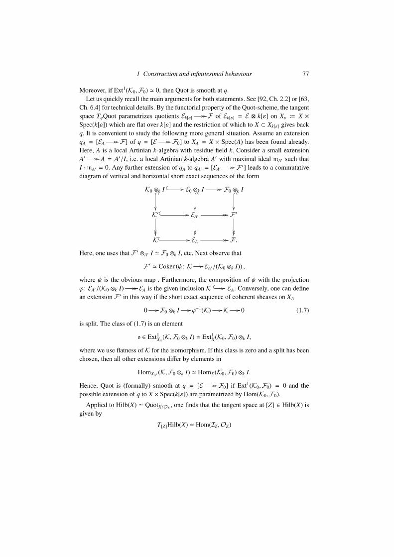
1 Construction and infinitesimal behaviour 77
Moreover, if Ext1(K0,F0) ' 0, then Quot is smooth at q.Let us quickly recall the main arguments for both statements. See [92, Ch. 2.2] or [63,
Ch. 6.4] for technical details. By the functorial property of the Quot-scheme, the tangentspace TqQuot parametrizes quotients Ek[ε] // //F of Ek[ε] = E k[ε] on Xε B X ×Spec(k[ε]) which are flat over k[ε] and the restriction of which to X ⊂ Xk[ε] gives backq. It is convenient to study the following more general situation. Assume an extensionqA = [EA // //F] of q = [E // //F0] to XA = X × Spec(A) has been found already.Here, A is a local Artinian k-algebra with residue field k. Consider a small extensionA′ // // A = A′/I, i.e. a local Artinian k-algebra A′ with maximal ideal mA′ such thatI · mA′ = 0. Any further extension of qA to qA′ = [EA′ // //F ′] leads to a commutativediagram of vertical and horizontal short exact sequences of the form
K0 ⊗k I //
_
E0 ⊗k I // // _
F0 ⊗k I _
K′ //
EA′ // //
F ′
K // EA // // F .
Here, one uses that F ′ ⊗A′ I ' F0 ⊗k I, etc. Next observe that
F ′ ' Coker (ψ : K // EA′/(K0 ⊗k I)) ,
where ψ is the obvious map . Furthermore, the composition of ψ with the projectionϕ : EA′/(K0 ⊗k I) // // EA is the given inclusion K
// EA. Conversely, one can definean extension F ′ in this way if the short exact sequence of coherent sheaves on XA
0 //F0 ⊗k I // ϕ−1(K) //K // 0 (1.7)
is split. The class of (1.7) is an element
o ∈ Ext1XA(K,F0 ⊗k I) ' Ext1X(K0,F0) ⊗k I,
where we use flatness of K for the isomorphism. If this class is zero and a split has beenchosen, then all other extensions differ by elements in
HomXA′ (K,F0 ⊗k I) ' HomX(K0,F0) ⊗k I.
Hence, Quot is (formally) smooth at q = [E // //F0] if Ext1(K0,F0) = 0 and thepossible extension of q to X × Spec(k[ε]) are parametrized by Hom(K0,F0).
Applied to Hilb(X) ' QuotX/OX, one finds that the tangent space at [Z] ∈ Hilb(X) is
given by
T[Z]Hilb(X) ' Hom(IZ ,OZ)

78 Chapter 3. Fano varieties of lines
and that Hilb(X) is smooth at [Z] if Ext1(IZ ,OZ) = 0. Now assume that Z ⊂ X is aregular embedding with normal bundle NZ/X . Then Hom(IZ ,OZ) ' H0(Z,NZ/X) andthe local to global spectral sequence, cf. [89, Ch. 3],
Ep,q2 = Hp(Z, Extq(IZ ,OZ))⇒ Extp+q(IZ ,OZ)
provides an exact sequence
H1(Z,NZ/X) // Ext1(IZ ,OZ) // H0(Z, Ext1(IZ ,OZ)) // H2(Z,NZ/X).
Furthermore, the local obstructions in Ext1(IZ ,OZ) to deform a smooth subvariety are alltrivial. Hence, the obstrucion space Ext1(IZ ,OZ) is indeed isomorphic to H1(Z,NZ/X).
Example 1.6. Let us test this in the case of G(m,P) ' HilbPm (P). We know that at[L = P(W)] ∈ G = G(m,P) the tangent space T[L]G is isomorphic to Hom(W,V/W)or, more globally, that TG ' Hom(S,Q) with S and Q as in (1.1). On the other hand,T[L]Hilb(P) ' Hom(IL,OL). And indeed, there is a natural isomorphism
Hom(W,V/W) ' Hom(IL,OL)
between the two descriptions obtained by applying Hom( ,OL) to the Koszul complex
· · · // ∧2(V/W)∗ ⊗O(−2) // (V/W)∗ ⊗O(−1) // IL // 0,
associated with the equations (V/W)∗ // V∗ for L = P(W), and by observing that
Hom((V/W)∗ ⊗O(−1),OL) ' (V/W) ⊗ H0(L,OL(1)) ' Hom(W,V/W).
Applied to the case [L] ∈ F(X,m) = HilbPm (X) for an m-plane L ⊂ X in a varietyX ⊂ P which is smooth (along L), one obtains the following result.
Proposition 1.7. Let L ⊂ X be an m-plane contained in a variety X ⊂ Pn+1 which issmooth along L. Then the tangent space T[L]F(X,m) of the Fano variety F(X,m) at thepoint [L] ∈ F(X,m) corresponding to L is naturally isomorphic to H0(L,NL/X):
T[L]F(X,m) ' H0(L,NL/X).
If H1(L,NL/X) = 0, then F(X,m) is smooth at [L] of dimension h0(L,NL/X).
Remark 1.8. There exists a relative version of the above. Assume X // S is a projec-tive morphism over a locally Noetherian base S and E is a coherent sheaf on X . Thenthe relative Quot-scheme π : QuotX /S/E // S parametrizes T -flat quotients ET // //F0
on X ×S T for all S -schemes T . It is a locally projective S -scheme with fibres π−1(s) =
QuotX/E |X , where X = Xs. In particular, the relative tangent space at a closed pointq = [E |X // //F0] ∈ QuotX/E |X ⊂ QuotX /S/E // S is the tangent space of the fibreπ−1(s) = QuotX/E |X , i.e.
Tqπ−1(s) ' TqQuotX/E |X ' HomX(K0,F0),

1 Construction and infinitesimal behaviour 79
where K0 = Ker(E |X // //F0). More interestingly, if locally in X no obstruction occurto deform E |X // //F0 and H1(Xs,Hom(K0,F0)) = 0, then π is smooth at q.
This applies to our situation. Consider the universal family X // |O(d)| of hyper-surfaces of degree d and let F(X ,m) // |O(d)| be the associated family of Fano vari-eties of m-planes in the fibres. Then the morphism F(X ,m) // |O(d)| is smooth at apoint [L] corresponding to an m-plane L ⊂ X in a smooth (along L) fibre X = Xs ifH1(X,NL/X) = 0.
To compute the normal bundle NL/X of an m-plane Pm ' L ⊂ X we use the shortexact sequence
0 //NL/X //NL/P|L //NX/P|L // 0 (1.8)
of locally free sheaves on L ' Pm, where we again assume that X is smooth or at leastsmooth along L.
The normal bundle NL/P can be readily computed by means of a comparison of theEuler sequences for L ' Pm and P = Pn+1. One finds NL/P ' O(1)⊕n+1−m. More pre-cisely, if L = P(W) ⊂ P = P(V), then NL/P ' OL(1) ⊗ (V/W).
If now X ⊂ P is a smooth (at least along L) hypersurface of degree d, then the exactsequence (1.8) becomes
0 //NL/X //OL(1)⊕n+1−m //OL(d) // 0. (1.9)
After the appropriate coordinate change, the surjection can be understood as given by∂iF, i = m + 1, . . . , n + 1. Indeed, assume that L = V(xm+1, . . . , xn+1). Then⊕m
i=0 OL(1)
//⊕n+1
i=0 OL(1)
(∂iF)
//⊕n+1
i=m+1 OL(1)
'
(∂iF)i=m+1,...,n+1
zz
TL // TP|L // NL/P
OL(d).
Observe that (1.9) has the following numerical consequences
det(NL/X) = OL((n + 1 − m) − d), rk(NL/X) = n − m, and
χ(NL/X) = χ(OL(1)) · (n + 1 − m) − χ(OL(d))
= (m + 1) · (n + 1 − m) −(m + d
d
),
which equals the right hand side of (1.6).For the case m = 1 and d = 3 this allows one to classify all normal bundles.

80 Chapter 3. Fano varieties of lines
Lemma 1.9. Let L ⊂ X be a line in a smooth (along L) cubic hypersuface X ⊂ Pn+1.Then NL/X ' OL(a1) ⊕ · · · ⊕OL(an−1), a1 ≥ · · · ≥ an−1, with
(a1, . . . , an−1) =
(1, . . . , 1, 0, 0) or
(1, . . . , 1, 1,−1).
Proof As L ' P1, any locally free sheaf is isomorphic to a direct sum of invertiblesheaves, so NL/X '
⊕OL(ai) with
∑ai = n − 3. On the other hand, the inclusion
NL/X ⊂ OL(1)⊕n yields ai ≤ 1. This immediately proves the result.
Definition 1.10. Lines with (ai) = (1, . . . , 1, 0, 0) and (ai) = (1, . . . , 1, 1,−1) are calledlines of the first type and of the second type, respectively.
The Gauss map is a useful tool to study lines of different types. Recall that the Gaussmap for a hypersurface X = V(F) ⊂ P B Pn+1 is the map
γX : P // P∗, x // [∂0F(x) : · · · : ∂n+1F(x)],
which is regular for smooth X. For d > 1 the morphism is not constant and hence finite.Then, also its restriction
γX : X // // X∗ B γX(X)
onto the dual variety X∗ is finite. Geometrically, γX maps x ∈ X to the embedded tangentspace TxX, Moreover, γX is generically injective as γX∗ γX = id, cf. [61, Ch. 12].
Exercise 1.11. Show that a line L ⊂ X is of the first type if and only if γX : L ∼− // γX(L)
is an isomorphism onto a smooth plane conic. It is of the second type if γX : L // γX(L)is a degree two covering of a line. Hint: Use (1.9) to show that γX |L is given by thequotient O⊕3
L// //OL(2) with kernel OL(−1) ⊕OL(−1) for lines of the first type and by
O⊕2L
// //OL(2) with kernel OL(−2) for lines of the second type. See [36, Sec. 6].
Note that in Lemma 1.9 for n = 2 there is in fact only one possibility, namely NL/X '
OL(−1). For n > 2 there are two cases and both can be geometrically realized, see [61,Prop. 6.30]. Obviously, (1, . . . , 1, 0, 0) describes the generic case. Equivalently, the setof lines of the second type
F2(X) B [L] | h0(L,NL/X(−1)) ≥ n − 2 ⊂ F(X)
is a proper closed subscheme. In fact, according to [36, Cor. 7.6], one has the followingupper bound for its dimension.
Lemma 1.12. For a smooth cubic hypersurface of dimension n, the locus F2(X) ⊂ F(X)of curves of the second type satisfies dim(F2(X)) ≤ n − 2. Consequently, the closed setof all x ∈ X contained in a line of the second type is of dimension at most n − 1.

1 Construction and infinitesimal behaviour 81
Proof As γX : X // X∗ is generically injective, the image of q : L2 B p−1(F2) // Xis a proper closed subscheme and, therefore, of dimension at most n − 1. Hence, asthe first projection p : L2 // // F2 is of relative dimension two, it suffices to show thatthe map q2 B q|L2 : L2 // q(L) ⊂ X is finite. For x ∈ q−1
2 (x) consider the mapιx : q−1
2 (x) // X, [L] // ιL(x), where ιL : L // L is the covering involution for the re-striction of the Gauss map γX |L : L // X∗, see Exercise 1.11. Thus, γX(ιx([L])) = γX(x)for all [L] ∈ q−1
2 (x) and, therefore, the image if ιx is finite. As L ∈ q−12 (x) is the unique
line through x and ιL(x), ιx is in fact injective and hence q−12 (x) is indeed finite.1
Exercise 1.13. Observe that L ⊂ X is of the second type if and only if the natural mapH0(L,NL/P(−1)) // H0(L,NX/P|L(−1)) is not surjective. Turn this into a description ofF2(X) ⊂ F(X) as the degeneracy locus of a natural map ξ : QF // S 2(S∗F), i.e. F2(X) =
[L] | ξ([L]) is not surjective . As rk(QF) = n and rk(SF) = 2, this yields the lowerbound dim(F2(X)) ≥ 2n − 4 −
(n3
), which is quite a bit smaller than n − 2 for n > 3.
Lemma 1.9 also shows that for a line P1 ' L ⊂ X contained in a smooth (along L)cubic hypersurface X ⊂ Pn+1 the Fano variety F(X) is smooth of dimension 2n − 4 at[L] ∈ F(X). Indeed, smoothness follows from Proposition 1.7 and H1(P1,O(a)) = 0for a = 0, 1. For the dimension observe that h0(L,
⊕O(ai)) = 2n − 4 in the two cases
(ai) = (1, . . . , 1, 0, 0) and (ai) = (1, . . . , 1, 1,−1).
Corollary 1.14. Let X ⊂ Pn+1 be a smooth cubic hypersurface, n ≥ 2. Then the Fanovariety of lines F(X) is smooth, projective, and of dimension
dim(F(X)) = 2n − 4.
Proof The preceding discussion essentially proves the claim. It remains to show thatF(X) is non-empty. For this consider the Fermat cubic X0 = V(x3
0 + · · · + x3n+1) which is
smooth for char(k) , 3. Then clearly the line L0 B V(x0 + x1, x2 + x3, x4, . . . , xn+1) iscontained in X0 and hence F(X0) , ∅. For char(k) = 3 with ξ =
√−1 ∈ k one may take
X0 B V(∑n
0 xix2i+1 + x3
0), see Section 1.2.2, and the line L0 B V(x0 − ξ x1, x2, . . . , xn+1).Of course, for the assertion one may assume k = k.
According to Remark 1.8, the vanishing H1(L0,NL0/X) = 0 not only proves that thefibre F(X0) of F(X ) // |O(3)| over [X0] ∈ |O(d)| is smooth at [L0] but that in factthe morphism is smooth at [L0]. In particular, the projective morphism F(X ) // |O(d)|is surjective which proves F(X) , ∅ for all cubics. Alternatively, one may combinedim(F(X0)) = 2n − 4 with Corollary 1.4 to conclude that the generic non-empty fibre isof dimension exactly 2n − 4. Hence, again by Corollary 1.4, F(X ) // |O(3)| has to besurjective, i.e. F(X) is non-empty for all X. Yet another, more direct argument will begiven in Remark 2.5.
1 There is a gap in the argument: What happens for ιL(x) = x?

82 Chapter 3. Fano varieties of lines
The existence of lines in cubic hypersurfaces has the following immediate conse-quence. The assumption on the field can be weakened. One only needs the existence ofone line contained in X.
Corollary 1.15. For any cubic hypersurface X ⊂ Pn+1 of dimension n > 1 defined overan algebraically closed field, there exists a rational dominant map of degree two
Pn // // X.
In particular, cubic hypersurfaces are unirational, cf. Remark 1.5.3.
Proof Pick a line L ⊂ X and consider the projectivization of the restricted tangentbundle P(TX |L) // L. A point in P(TX |L) is represented by a tangent vector 0 , v ∈ TxX,which then defines a unique line Lv ⊂ P passing through x with TxL ⊂ TxX spanned byv. Then, either the line Lv is contained in X or, and this is the generic case, it is not andthen Lv intersects X in a unique point yv ∈ X with the property that the scheme theoreticintersection Lv ∩ X is 2x + yv. Note that yv = x can occur.
This defines a rational map
P(TX |L) // // X , v // yv, (1.10)
which is regular on a dense open subset intersecting each fibre P(TxX), x ∈ L, unless Xcontains a hyperplane.
Now, pick a point y ∈ X \ L in the image and consider the cubic curve yL ∩ X. Ifit is of the form L ∪ Q such that the quadric Q does not contain L, then there exist atmost two lines y ∈ Li, i = 1, 2, that intersect L and are tangent to X at the intersectionpoint. They are given by the (at most) two points of the intersection L ∩ Q. In otherwords, the generic non-empty fibre of v // yv would consists of at most two points. Inparticular, for dimension reasons, P(TX |L) // // X would be dominant. To show that
yL∩ X = L∪ Q with L 1 Q for generic choice of y, take any tangent vector v ∈ TxPn+1,
x ∈ L, not contained in TxX. Then the line Lv will not be tangent to X at x and, therefore,L 1 Q for the residual quadric of L ⊂ LvL∩X. But then any y ∈ Q will have the property.Hence, the rational map (1.10) is generically of degree two and dominant.
Remark 1.16. The restriction of the map (1.10) to the fibre over one point x ∈ L yieldsa rational map
P(TxX) // X.
The map has indeterminacies in all tangent directions v for which the line Lv is containedin X. As the line Lv is determined by the two points x, yv as soon as x , yv, the map isinjective on the open subset of tangent directions with Lv ∩ X = 3x.
In Section 5.?? we shall describe the indeterminacy locus explicitly for n = 3. See

2 Global properties and a geometric Torelli theorem 83
Remark 1.5.3 for an alternative argument proving unirationality of cubic hypersurfacescontaining a linear subspace Pn−2 and, in fact, rationally for n ≥ 7.
Remark 1.17. There is a general expectation (conjecture of Debarre–de Jong) that ford ≤ n+1 and char(k) = 0 or at least char(k) ≥ d the Fano variety of lines F(X) is smoothof the expected dimension 2n − d − 1. For d ≤ 6 this has been proved in characteristiczero in [17] for which we also refer for further references. See also [61, Prop. 6.40],where the claim is reduced to the case d = n + 1.
Remark 1.18. Note that for m ≥ 2 and an m-plane L ⊂ X contained in a smooth(along L) hypersurface X of degree d such that NL/X '
⊕O(ai) the Fano variety
F(X,m) is smooth at [L] of dimension∑
h0(Pm,O(ai)). However, in contrast to locallyfree sheaves on P1, there is a priori no reason why NL/X on L ' Pm should be a directsum of invertible sheaves. Also the dimension of F(X,m) is harder to control as othercohomology groups Hi(L,NL/X) enter the picture.
2 Global properties and a geometric Torelli theorem
No information is lost when passing from a smooth cubic hypersurface to its Fano va-riety of lines. More precisely, two cubic hypersurfaces of dimension 3 ≤ n , 4 areisomorphic if and only if their Fano varieties are isomorphic. For cubic fourfolds thePlücker polarization of the Fano variety has to be taken into account and, of course, forsmooth cubic surfaces the Fano variety, consisting just of 27 reduced points, the resultfails.
2.1 Recall that det(S∗) ' O(1)|G for the Plücker embedding G // P(
∧m+1 V). Thefollowing result is [4, Prop. 1.8].
Lemma 2.1. For a smooth cubic hypersurface X ⊂ Pn+1 the canonical bundle ωF of theFano variety of lines F = F(X) ⊂ G(1,P)
// P(n+2
2 )−1 is
ωF ' O(4 − n)|F .
Proof As the Fano variety is the zero set F = V(sF) ⊂ G(1,P) of a regular sectionsF ∈ H0(G, S 3(S∗)), the normal bundle sequence for F ⊂ G takes the form
0 // TF // TG|F // S 3(S∗)|F // 0
and the adjunction formula yields
ωF = det(T ∗F ) '(ωG ⊗ det(S 3(S∗))
)|F .
As TG ' Hom(S,Q), one has ωG ' det(S ⊗Q∗) ' det(S)n+1−m ⊗ det(Q∗)m+1 ' O(−n−

84 Chapter 3. Fano varieties of lines
2)|G. Thus, it remains to prove that det(S 3(S)) ' det(S)6 which one deduces from acomputation involving the splitting principle: Write formally S = L0 ⊕ L1 and observeS 3(L0 ⊕ L1) ' L3
0 ⊕ (L20 ⊗ L1) ⊕ (L0 ⊗ L2
1) ⊕ L31.
Thus, for smooth cubic threefolds X ⊂ P4 the Fano variety of lines F(X) is a smoothprojective surface with very ample canonical bundle, in particular F(X) is of generaltype. For smooth cubic fourfolds X ⊂ P5 the Fano variety F(X) has trivial canonicalbundle ωF ' OF and we will later see that it is a four-dimensional hyperkähler mani-fold. Eventually, for n > 4 the Fano variety becomes a Fano variety in the sense that itsanti-canonical bundle ω∗X is (very) ample. In short:
ωF(X) =
ample if n = 3,
trivial if n = 4,
anti-ample if n > 4.
We will later determine the (rational) cohomology of F(X) for any smooth cubic hy-persurface X ⊂ Pn+1, cf. Section 3.4. At least in characteristic zero, the positivity prop-erty of the canonical bundleωF(X) already implies certain vanishings, e.g. Hq(F(X),O) =
0 for n > 4 and q > 0. See also Corollary 3.8 for an alternative approach. This allowsone to prove the following result for n > 4.
Corollary 2.2. Let F = F(X) be the Fano variety of lines in a smooth cubic hypersur-face X ⊂ Pn+1 over C. Then H1(F,Z) = 0 for n ≥ 4 and, in particular, Pic0(F) = 0. Forn ≥ 5 one has Pic(F) ' H2(F,Z)(1).
In fact, the vanishing of Pic0(F) holds true in arbitrary characteristic, as Kodairavanishing holds for liftable varieties [51].
Apart from the Fano variety of lines on a cubic surface, all others are connected, see[4, Thm. 1.16] and [8, Thm. 6]. This leads to the following strengthening of Corollary1.14.2
Proposition 2.3. Let X ⊂ Pn+1 be a smooth cubic hypersurface of dimension n > 2.Then F(X) is an irreducible, smooth, projective variety of dimension 2n − 4.
Proof More generally, Barth and Van den Ven [8] prove that the Fano variety of linesF(X) on any, not necessarily smooth, hypersurface X ⊂ Pn+1 of degree d is connectedif d < 2(n − 1). They argue by bounding the dimension of the ramification locus (of theStein factorization) of L // X. Altman and Kleiman [4] use instead the Koszul complex
· · · // ∧2(S 3(S)) // S 3(S) //OG //OF(X) // 0.
2 One could think of applying the Fulton–Lazarsfeld connectivity [110, Thm. 7.2.1], to prove its connectivitywhenever dim(F(X,m)) > 0. However, this would need the ampleness of S d(S∗) which is just wrong.

2 Global properties and a geometric Torelli theorem 85
The induced spectral sequence
Ep,q1 = Hq(G,
∧−p (S 3(S)))⇒ Hp+q(F(X),OF(X))
combined with generalized Bott vanishing results for Grassmann varieties:
Hp(G,∧p (S 3(S))) = 0 for all p , 0
yield H0(G,OG) ∼− // H0(F(X),OF(X)). Hence, F(X) is connected.
For alternative arguments see Exercise 2.6, for n ≥ 4, and Example 3.12.
Exercise 2.4. Let X ⊂ Pn+1 be cubic hypersurface and assume m is an integer withm2 + 11m ≤ 6n. Show that there exists a linear subspace Pm ⊂ X ⊂ Pn+1 of dimensionm contained in X.
Remark 2.5. For n > 2, the universal line L = P(S |F(X)) // F(X) maps onto X or,equivalently, through every point x ∈ X there exists at least one line x ∈ L ⊂ X, possiblydefined only over a finite extension of the residue field of x.
To prove this claim we may assume that k is algebraically closed. For a fixed pointx ∈ X, let Pn ⊂ Pn+1 be a hyperplane not containing x. We may assume x = [1 :0 : · · · : 0] and Pn = V(x0). If X = V(F), then the projective tangent space is thehyperplane TxX = V(
∑xi ∂iF(x)) and any line x ∈ L ⊂ TxX has intersection multiplicity
multx(X, L) ≥ 2. For dimension reasons, there exists a point
y ∈ Pn ∩ TxX ∩ X ∩ V(∂0F).
Then let L = xy be the line connecting the two points. We may choose coordinates suchthat y = [0 : 1 : 0 : · · · : 0] and then F|L is the polynomial F(x0, x1, 0, . . . , 0). By defini-tion ∂0F(y) = 0 and by the Euler equation also ∂1F(y) = 0. Therefore, multy(X, L) ≥ 2.However, a line L ⊂ Pn+1 intersecting a cubic hypersurface X ⊂ Pn+1 in two distinctpoints with multiplicity at least two at both points is contained in X.
Alternatively, to prove surjectivity, one may first take hyperplane sections to reduceto the case of smooth cubic threefolds Y ⊂ P4. Then the result follows from [36, Cor.8.2]. Another more direct argument can be found in [37, Lem. 2.1]. The above proof istaken from [72].
Note that the argument also shows that the fibre of L // X over x has the expecteddimension n−3 if and only if the intersection Pn ∩TxX∩X∩V(∂0F) is of this expecteddimension.
Exercise 2.6. Assume n ≥ 4 and observe that then Pn ∩ TxX ∩ X ∩ V(∂0F) in Remark2.5 is connected by Bertini’s theorem. Deduce from this that F(X) is connected, thusproving Proposition 2.3 again for cubic hypersurfaces of dimension n ≥ 4.
Remark 2.7. Mapping a point ([L], x) ∈ L to the tangent direction of L at x ∈ Lyields a morphism $ : L // P(TX). On each fibre of the projection p : L // F(X) it is
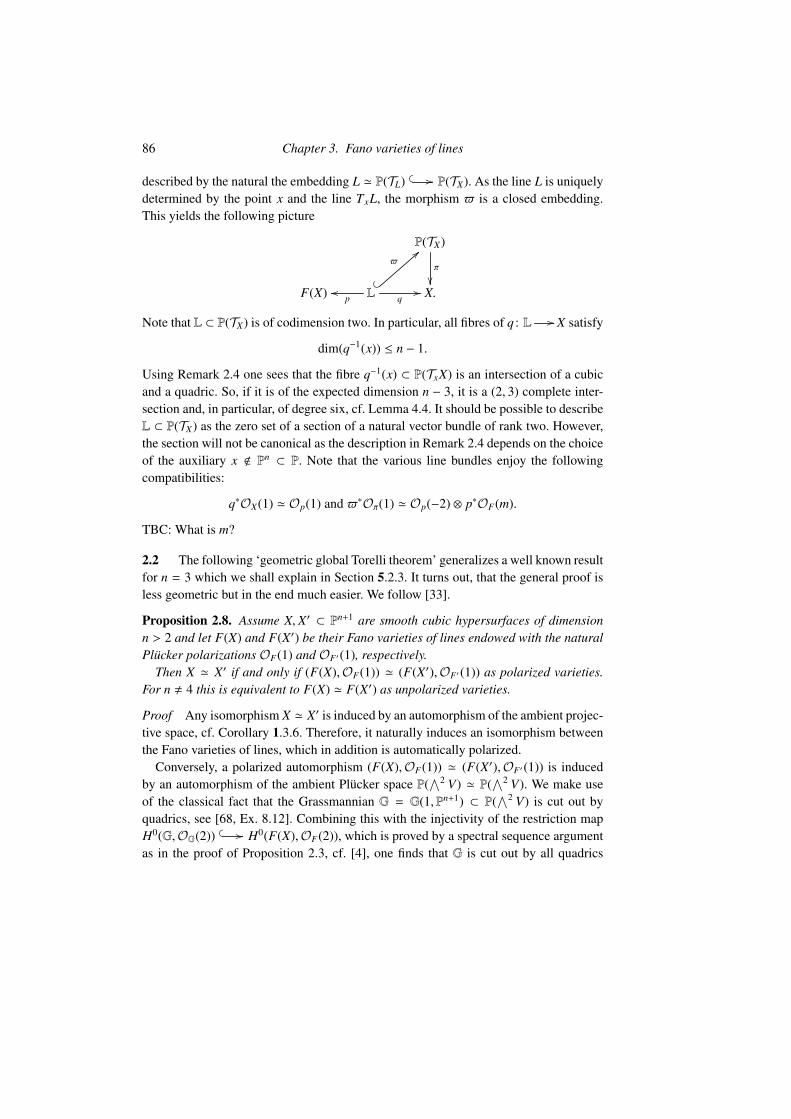
86 Chapter 3. Fano varieties of lines
described by the natural the embedding L ' P(TL) // P(TX). As the line L is uniquely
determined by the point x and the line TxL, the morphism $ is a closed embedding.This yields the following picture
P(TX)
π
F(X) Lp
oo.
$
==
q// X.
Note that L ⊂ P(TX) is of codimension two. In particular, all fibres of q : L // X satisfy
dim(q−1(x)) ≤ n − 1.
Using Remark 2.4 one sees that the fibre q−1(x) ⊂ P(TxX) is an intersection of a cubicand a quadric. So, if it is of the expected dimension n − 3, it is a (2, 3) complete inter-section and, in particular, of degree six, cf. Lemma 4.4. It should be possible to describeL ⊂ P(TX) as the zero set of a section of a natural vector bundle of rank two. However,the section will not be canonical as the description in Remark 2.4 depends on the choiceof the auxiliary x < Pn ⊂ P. Note that the various line bundles enjoy the followingcompatibilities:
q∗OX(1) ' Op(1) and $∗Oπ(1) ' Op(−2) ⊗ p∗OF(m).
TBC: What is m?
2.2 The following ‘geometric global Torelli theorem’ generalizes a well known resultfor n = 3 which we shall explain in Section 5.2.3. It turns out, that the general proof isless geometric but in the end much easier. We follow [33].
Proposition 2.8. Assume X, X′ ⊂ Pn+1 are smooth cubic hypersurfaces of dimensionn > 2 and let F(X) and F(X′) be their Fano varieties of lines endowed with the naturalPlücker polarizations OF(1) and OF′ (1), respectively.
Then X ' X′ if and only if (F(X),OF(1)) ' (F(X′),OF′ (1)) as polarized varieties.For n , 4 this is equivalent to F(X) ' F(X′) as unpolarized varieties.
Proof Any isomorphism X ' X′ is induced by an automorphism of the ambient projec-tive space, cf. Corollary 1.3.6. Therefore, it naturally induces an isomorphism betweenthe Fano varieties of lines, which in addition is automatically polarized.
Conversely, a polarized automorphism (F(X),OF(1)) ' (F(X′),OF′ (1)) is inducedby an automorphism of the ambient Plücker space P(
∧2 V) ' P(∧2 V). We make use
of the classical fact that the Grassmannian G = G(1,Pn+1) ⊂ P(∧2 V) is cut out by
quadrics, see [68, Ex. 8.12]. Combining this with the injectivity of the restriction mapH0(G,OG(2))
// H0(F(X),OF(2)), which is proved by a spectral sequence argumentas in the proof of Proposition 2.3, cf. [4], one finds that G is cut out by all quadrics

3 Cohomology and motives 87
containing F(X) or, alternatively, containing F(X′). In other words, F(X) ' F(X′) isinduced by an automorphism of the ambient Grassmannian
F(X)
'
// G
'
// P(∧2V)
'
F(X′) // G
// P(∧2V).
However, any automorphism of G compatible with its Plücker embedding is induced byan automorphism of P(V), see [35].
For n , 4, the canonical bundle ωF ' OF(4 − n) is a non-trivial, possibly negative,multiple of the Plücker polarization OF(1). Clearly, any isomorphism F(X) ' F(X′) re-spects the canonical bundle. Using that Pic(F(X)) is torsion free for n > 4, this impliesthat any isomorphism F(X) ' F(X′) is automatically polarized. To see that Pic(F(X)) istorsion free, observe that for a torsion line bundle L one has χ(F(X), L) = χ(F(X),O) =
1, as F(X) is a Fano variety for n > 4, with Hi(F(X), L) = 0 for i > 0 by Kodairavanishing (which holds also in positive characteristic zero, as F(X) is liftable to charac-teristic zero [51]) and, therefore, L ' O.3 For n = 3, the fact that ωF ' O(1)|F sufficesto conclude.
The proof above shows more, namely that any (polarized) isomorphism F(X) 'F(X′) is induced by an isomorphism X ' X′. For n = 3 we will provide a differentproof which relies on an isomorphism between the restriction of the tautological bundleSF and the tangent sheaf TF , see Proposition 5.2.8.
Corollary 2.9. For a smooth cubic hypersurface X ⊂ Pn+1 of dimension n , 4 the groupof automorphisms Aut(F(X)) of its Fano variety of lines is finite and H0(X, TF(X)) = 0.The vanishing holds as well for n = 4.
Proof By the arguments in the above proof, for n , 4 any automorphism F(X) ' F(X)is induced by an automorphism of X. As Aut(X) is finite for all cubic hypersurfaces ofdimension by Corollary 1.3.6 this proves the assertion. The tangent space of the groupscheme Aut(F(X)) is H0(F(X), TF(X)), which therefore has to vanish. For n = 4 oneargues using polarized automorphisms.
3 Cohomology and motives
According to Proposition 2.8 the Fano variety F(X) of lines contained in a smooth cubichypersurface X determines the hypersurface. Therefore, essentially all and, in particular,3 Thanks to S. Stark for the argument. Alternatively, one can use [48]. As an aside, Pic(F(X)) is also torsion
free for n = 4, as then F(X) is a hyperkähler manifold, see Chapter ??.?? and, therefore, Pic(F(X) 'NS(F(X)), cf. Remark 3.10.

88 Chapter 3. Fano varieties of lines
all cohomological and motivic information about X should be encoded by F(X). In thissection we shall study the cohomology of F(X) and we shall do this by first looking atthe motive of F(X).
3.1 As the Fano variety F(X) itself, its motive is an interesting object to study. Now,the motive of F(X) may mean various things. Here, we are interested in the class [F(X)]of F(X) in the Grothendieck ring of varieties K0(Vark) and in its motive h(F(X)) in thecategory Mot(k) of rational Chow motives.
Recall that the Grothendieck ring K0(Vark) of varieties over a field k is by definitionthe abelian group generated by classes [Y] of quasi-projective varieties modulo onerelation [Y] = [Z] + [U], the scissor relation, for any closed subset Z ⊂ Y with opencomplement U = Y \ Z. Then K0(Vark) becomes a ring with multiplication given by theproduct [Y] · [Y ′] = [Y × Y ′]. The Lefschetz motive is the class ` B [A1] of the affineline. An important consequence of the scissor relation is the fact that [Y] = [F] · [Z] fora Zariski locally trivial fibration Y // Z with fibre F. See for example [5, Ch. 13] or[32, Ch. 2] for more details.
In [66], the class [F(X)] ∈ K0(Vark) is related to the class [X[2]] ∈ K0(Vark) of theHilbert scheme X[2] of subschemes of X of length two. The Hilbert scheme can beobtained as the blow-up of the symmetric product X(2) B (X×X)/S2 along the diagonalX ' ∆ ⊂ X(2). Hence, in K0(Vark) one has
[X[2]] − [Pn−1] · [X] = [X(2)] − [X]. (3.1)
Proposition 3.1 (Galkin–Shinder). Let X ⊂ Pn+1 be a smooth cubic hypersurface. Thenin K0(Vark)
[X[2]] = [Pn] · [X] + `2 · [F(X)]
and
[X(2)] = (1 + `n) · [X] + `2 · [F(X)].
Proof We follow closely the argument in [66], where one also finds a version forsingular cubics.
Consider the universal family F(X) Loo // X of lines contained in X. AsL // F(X) is the P1-bundle P(S |F(X)) // F(X), its class in K0(Vark) is given by
[L] = [P1] · [F(X)]. (3.2)
Similarly, let G = G(1,P) LGoo // P be the universal family of lines in P andlet LG |X be the pre-image of X under the second projection. Then LG|X parametrizespairs (x, L) consisting of a line L ⊂ P and a point x ∈ X ∩ L. It can also be describedas the Pn-bundle P(TP|X) // X, cf. the construction in the proof of Corollary 1.15. This

3 Cohomology and motives 89
shows that in K0(Vark) one has
[LG |X] = [Pn] · [X]. (3.3)
Next, consider the morphism
LG|X \ L // X[2]
that sends (x, L) to the residual intersection [(L ∩ X) \ x] ∈ X[2]. It is inverse to themorphism
X[2] \ L[2] // LG|X
that sends [Z] ∈ X[2] to (x, LZ), where LZ ⊂ P is the unique line containing the lengthtwo-subscheme Z ⊂ P and x is the residual point of the inclusion Z ⊂ X∩LZ . Here, L[2] isthe relative symmetric product of the universal line p : L // F(X), which equivalentlycan be described as the relative Hilbert scheme of subschemes of length two in the fibresof p or, still equivalently, as L[2] ' P(S 2(S∗|F(X))) // F(X). In particular,
[L[2]] = [P2] · [F(X)] (3.4)
in K0(Vark). The isomorphism
LG|X \ L ' X[2] \ L[2]
together with (3.2), (3.3), and (3.4) yields the first assertion. The second follows from(3.1).
Remark 3.2. A closer inspection reveals, see [156, Prop. 2.9] for further details, thatthe construction in the proof above leads to the following picture:
BlL(LG|X) ' BlL[2] (X[2])
yy &&
E
⋃
P2vv P1 ((
LG|X L⊃P1
((
L[2] ⊂
P2
vv
X[2]
F(X).
Here, E is the exceptional divisor of the two blow-up morphisms. In fact, BlL(LG|X) 'BlL[2] (X[2]) is an irreducible component of the incidence variety
(x, L,Z) | x ∈ L ∩ X, Z ⊂ L ∩ X ⊂ X × LG|X × X[2].
Standard formulae for cohomology or motives of smooth blow-ups and projective bun-dles can be applied. For example, for the category of rational Chow motives Mot(k) one

90 Chapter 3. Fano varieties of lines
knows that
h(BlL(LG|X)) ⊕ h(L) ' h(LG |X) ⊕ h(E)
and
h(BlL[2] (X[2])) ⊕ h(L[2]) ' h(X[2]) ⊕ h(E),
see [5, 128]. This can be combined with h(LG |X) '⊕n
i=0 h(X)(−i) and
h(L) ' h(F(X)) ⊕ h(F(X))(−1)
h(L[2]) ' h(F(X)) ⊕ h(F(X))(−1) ⊕ h(F(X))(−2).
Here, h(X)(−i) B h(X) ⊗ (P1, [P1 × x])⊗i is the twist with the i-th power of the Lef-schetz motive. The isomorphism BlL(LG|X) ' BlL[2] (X[2]) then yields a formula which,if cancellation holds in Mot(k), would look like this:
h(F(X))(−2) ⊕n⊕
i=0
h(X)(−i) ' h(X[2]). (3.5)
That cancellation really holds in this case was proved in [108], so (3.5) holds true. Theformula can be combined with the isomorphism
h(X[2]) ' S 2h(X) ⊕
n−1⊕i=1
h(X)(−i), (3.6)
which shows that finite-dimensionality of h(X) in the sense of Kimura implies finite-dimensionality of h(F(X)), cf. [108, Thm. 4].4
One also expects the following isomorphism to hold:
h(F(X))(−2) ⊕ h(X) ⊕ h(X)(−n) ' S 2h(X), (3.7)
which would follow from the above if cancellation holds. Using the decompositionh(X) ' hn(X)pr ⊕
⊕ni=0 Q(−i), cf. Remark 1.1.7, and cancellation, this then becomes
h(F(X))(−2) ⊕ Q(−n) ' S 2h
n(X)pr ⊕
n−1⊕i=1
hn(X)pr(−i) ⊕
⊕0<i≤ j<n
Q(−i − j). (3.8)
Here, Q(1) is the Tate motive (Spec(k), id, 1), the dual of the Lefschetz motive.
4 It is not known whether smooth cubic hypersurfaces of dimension 5 , n > 3 are Kimura finite-dimensional. For n = 3 the argument will be given in Section 5.3. Finite-dimensionality is also knownfor n = 5 (with thanks to R. Laterveer for the explanation).

3 Cohomology and motives 91
3.2 Combining the information obtained from the description of F(X) ⊂ G(1,P) asthe zero set V(sF) and the description of its class [F(X)] ∈ K0(Vark), one can deduce thefollowing numerical information, see [4, Prop. 1.6] and [66, Cor. 5.2]. The case n = 3goes back to [22].
Proposition 3.3 (Altman–Kleiman, Galkin–Shinder). Let X ⊂ Pn+1 be a smooth cubichypersurface and F(X) its Fano variety of lines considered with its projective embed-ding F(X)
// G(1,P) // P(
n+22 )−1. Then degree and Euler number of F(X) are given
by the following formulae
deg(F(X)) = 27 ·(2n − 4)!
n! · (n − 1)!· (3n2 − 7n + 4) (3.9)
and
e(F(X)) =e(X) · (e(X) − 3)
2=
22n+4 + (−2)n+2 · (6n + 1) + 3n · (3n + 1) − 2018
. (3.10)
Proof As a special case of (1.3), we know that [F(X)] = c4(S 3(S∗)) in the cohomologyor in the Chow ring of G. Writing formally S∗ = L0 ⊕ L1 and S 3(S∗) = L3
0 ⊕ (L20 ⊗ L1)⊕
(L0 ⊗ L21) ⊕ L3
1 allows one to compute
c4(S 3(S∗)) = 9 · (5 `20`
21 + 2 (`3
0`1 + `0`31))
= 9 · (2 c1(S∗)2 + c2(S∗)) · c2(S∗),
where `i = c1(Li). Hence,
deg(F(X)) = 9∫G
c1(S∗)2n−4 · (2 c1(S∗)2 + c2(S∗)) · c2(S∗).
Using standard Schubert calculus (Pieri’s and Gambelli’s formulae), this is turned in [4]into a rather complicated formula which then can be simplified to the above.
In principle, the second assertion can also be deduced by Schubert calculus, as
e(F(X)) =
∫F(X)
c2n−4(TF(X)) =
∫G
(c(TG)
c(S 3(S∗))
)2n−4· c4(S 3(S∗)).
However, there is a more illuminating way of doing this. Indeed, taking Euler numbersin the second equation in Proposition 3.1 yields
e(X(2)) = 2 · e(X) + e(F(X)),
where we use the additivity and the multiplicativity of the Euler number and e(`n) = 1,cf. [20]. However, taking cohomology commutes with taking symmetric products, i.e.H∗(X(n)) = S nH∗(X) (say with coefficients in a field of characteristic zero), cf. [74, Prop.

92 Chapter 3. Fano varieties of lines
5.2.3] or [115]. Therefore, e(X(2)) =(
e(X)+12
).5 This proves the first equality in (3.10) and
the second follows from (1.6) in Chapter 1.
Remark 3.4. Recall from Section 1.1.4 that the Euler numbers e(Xn) of all smoothcubic hypersurfaces Xn ⊂ P
n+1 can also be described by the generating series∞∑
n=0
e(Xn) zn+1 =3 z
(1 − z)2 (2 z + 1).
A formal computation using Mathematica6 reveals∞∑
n=0
e(F(Xn)) zn+1 =27 (1 − 2 z) z3
(−1 + z)3 (1 + 2 z)2 (−1 + 4 z),
but a conceptual understanding in the sense of Theorem 1.1.11 is not known.
n ωF(X) dim(F(X)) deg(F(X)) e(F(X))
2 O 0 27 273 O(1) 2 45 274 O 4 108 3245 O(−1) 6 297 702
3.3 The computation of the Euler number is only a shadow of the full cohomologicalinformation available. There are various ways to unpack the information encoded bythe above considerations. We shall focus on the Hodge theoretic content and so assumefrom now on that k = C.
To start, let HSZ,n be the additive category of polarizable, pure Hodge structures ofweight n.7 Recall that the Tate twist defines an equivalence
HSZ,n∼− // HSZ,n−2, H // H(1) B H ⊗ Z(1),
5 The closed formula due to MacDonald says
∞∑n=0
e(X(n)) zn = (1 − z)−e(X) = exp
e(X) ·∞∑
r=1
zr/r
,which is the geometric analogue of the well-known equality
∑∞n=0 |X
(n)(Fq)| zn = exp(∑|X(Fqr )| zr/r
)for
the Zeta function of a variety over a finite field Fq and which generalizes to an equality for the Poincarépolynomial
∞∑n=0
∑i
(−1)ibi(X(n)) yi
zn =(1 − y1t)b1(X) · (1 − y3t)b3(X) · · ·
(1 − t)b0(X) · (1 − y2t)b2(X) · · ·.
6 . . . with thanks to P. Magni.7 The notation is borrowed from [60].

3 Cohomology and motives 93
where Z(1) = (2πi)Z is the pure Hodge structure of weight (−1,−1) geometricallyrealized by the dual of H2(P1,Z). We let HSZ =
⊕HSZ,n be the additive category of
graded pure, integral Hodge structures and denote its Grothendieck group by K0(HSZ).By definition, this is the group generated by isomorphism classes of integral polarizableodge structures with the condition that [H] + [H′] = [H ⊕ H′]. In particular, two Hodgestructures H and H′ define the same class [H] = [H′] in K0(HSZ) if and only if thereexists a Hodge structure H0 such that H ⊕ H0 ' H′ ⊕ H0.
Recall that according to [20], K0(VarC) can also be described as the quotient of thefree abelian group generated by isomorphism classes of smooth projective varieties bythe relation
[BlZ(Y)] + [Z] = [Y] + [E]
for every blow-up BlZ(Y) // Y of a smooth projective variety Y along a smooth pro-jective subvariety Z ⊂ Y with exceptional divisor E. Using that for each such smoothblow-up there exists an isomorphism of polarizable integral Hodge structures
H∗(BlZ(Y),Z) ⊕ H∗(Z,Z) ' H∗(Y,Z) ⊕ H∗(E,Z),
one finds that there exists a ring homomorphism
K0(VarC) // K0(HSZ), [X] // H∗(X,Z). (3.11)
Under this map, ` = [A1] = [P1] − [pt] is sent to Z(−1).
Corollary 3.5. Let X ⊂ Pn+1 be a smooth cubic hypersurface. Then in K0(HSZ) thefollowing equality holds
[H∗(F(X),Z)] + [H∗(Pn,Z)(2)] · [H∗(X,Z)] = [H∗(X[2],Z)(2)]. (3.12)
Proof Apply (3.11) to Proposition 3.1 and twist by Z(2).
Next consider the natural functor
HSZ //HSQ, H // H ⊗Z Q,
to the category of graded pure, polarizable, rational Hodge structures. It induces a linearmap
K0(VarC) // K0(HSZ) // K0(HSQ). (3.13)
As the category of graded pure, polarizable, rational Hodge structures HSQ is semi-simple (cf. [132, Cor. 2.12]), the natural map
HSQ // K0(HSQ)
is injective, i.e. two rational Hodge structures H and H′ are isomorphic if and only

94 Chapter 3. Fano varieties of lines
if [H] = [H′] in K0(HSQ).8 Thus, (3.12) becomes an isomorphism of rational Hodgestructures
H∗(F(X),Q) ⊕ (H∗(Pn,Q) ⊗ H∗(X,Q)) (2) ' H∗(X[2],Q)(2).
There is a shortcut to arrive at this isomorphism by just applying cohomology to (3.5),i.e. using the commutativity of the diagram
(SmProj(C))
// Mot(C)
K0(VarC) // K0(HSZ) // K0(HSQ).
Similarly, either by applying cohomology to (3.6) or by using (3.13), one obtains anisomorphism of Hodge structures
H∗(X[2],Q) ' S 2H∗(X,Q) ⊕n−1⊕i=1
H∗(X,Q)(−i).
Altogether this leads to the isomorphism of Hodge structures
H∗(F(X),Q) ⊕ H∗(X,Q)(2) ⊕ H∗(X,Q)(2 − n) ' S 2(H∗(X,Q))(2) (3.14)
and, after decomposing into primitive parts,
H∗(F(X),Q) ⊕ Q(2 − n) (3.15)
'
n−1⊕i=1
Hn(X,Q)pr(2 − i) ⊕⊕
0<i≤ j<n
Q(2 − i − j)
⊕
S 2(Hn(X,Q)pr)(2) for n ≡ 0 (2)∧2(Hn(X,Q)pr)(2) for n ≡ 1 (2),
cf. [66]. The latter can also be obtained by taking cohomology of (3.8). In particular,for the middle cohomology of the Fano variety the formula yields
H2n−4(F(X),Q) = Q(2−n)⊕n−2⊕
S 2(Hn(X,Q)pr)(2) for n ≡ 0 (2)∧2(Hn(X,Q)pr)(2) ⊕ Hn(X,Q)pr(1 − n2 ) for n ≡ 1 (2).
Corollary 3.6. For the general smooth cubic hypersurface X ⊂ Pn+1 the Hodge conjec-ture holds for F(X) in the middle degree 2n − 4 and dim Hn−2,n−2(F(X),Q) = n − 3.
Proof
8 Injectivity does not hold for integral Hodge structures. Indeed, there exist elliptic curves E, E′, and E0 suchthat E and E′ are non-isomorphic but E × E0 ' E′ × E0, see [146]. In this case [H1(E,Z)] = [H1(E′,Z)]in K0(HSZ), but H1(E,Z) and H1(E′,Z) are non-isomorphic Hodge structures. Thanks to B. Moonen forthe reference.

3 Cohomology and motives 95
3.4 Proposition 3.1 or, alternatively (3.15), allows one to compute all Betti and Hodgenumbers of F(X).
Corollary 3.7. The χy-genus of the Fano variety of lines F(X) of a smooth cubic hyper-surface X ⊂ Pn+1 is given by
χy(F(X)) =χy(X) − 2yn − 1
2y2 · χy(X).
In principle, it should be possible to combine this with Hirzebruch’s formula for thegenerating series
∑∞n=0 χy(Xn) zn+1 of all χy-genera of cubic hypersurfaces, see Theorem
1.1.11, to express∑∞
n=0 χy(F(Xn)) zn+1 as a rational function, cf. Remarks 3.4 and 3.13.
Before making some of the computations explicit in low-dimensional cases, we shalldraw a few further consequences of (3.15).
Corollary 3.8. Let X be a smooth cubic hypersurface of dimension n.
(i) If n is even, then H∗(X,Q) = Hev(X,Q) and H∗(F(X),Q) = Hev(F(X),Q).(ii) If n is odd, then H∗(X,Q) = Hev(X,Q) ⊕ Hn(X,Q) and
H∗(F(X),Q) = Hev(F(X),Q) ⊕n−1⊕i=1
Hn(X,Q)pr(2 − i).
The description of the first cohomology yields an alternative proof of Corollary 2.2.
Corollary 3.9. Assume n ≥ 4. Then the Picard variety Pic0(F(X)) of the Fano varietyof lines F(X) on a smooth cubic hypersurface X ⊂ Pn+1 is trivial.
Proof Indeed, as Hodd(F(X),Q) is trivial for even n and otherwise Hodd(F(X),Q) '⊕n−1i=1 Hn(X,Q)pr(2 − i), one finds H1(F(X),Q) = 0 for n ≥ 4. Hence, H0,1(F(X)) = 0
which implies that Pic0(F(X)) is trivial.
Remark 3.10. In fact, the F(X) are known to be simply connected for n ≥ 4.9 For n = 4it is due to [16] and for n > 4 the result follows from [147]. See [48, Prop. 1& Ex. 3.3],where it is also shown that Pic(F(X)) ' Z ·OF(1) for n > 4.
Alternatively, one can use the fact that for n > 4 the Fano variety of lines F(X) isa Fano variety, i.e. has negative canonical bundle. Quite generally, due to results ofCampana and Kollár rationally connected varieties Z are simply connected, cf. [45, 46].Roughly, at least in characteristic zero, this follows from the observation that any finiteétale cover π : Z // Z would again be Fano and, therefore, 1 = χ(Z,O) = χ(Z,O) ·deg(π).
9 I am indebted to R. Laterveer and S. Stark for pointing this out to me and providing the references.

96 Chapter 3. Fano varieties of lines
The middle cohomology Hn(X,Q) of the cubic hypersurface X carries the most infor-mation. As we will see again and again, for the Fano variety of lines it is the cohomologyin degree n − 2, which is below the middle for all n. And indeed, the next result saysthat the two are intimately related. See Section 4 for an alternative argument.
Corollary 3.11. Let X be a smooth cubic hypersurface of dimension n.
(i) If n is even, then
Hn−2(F(X),Q) ' Hn(X,Q)pr(1) ⊕⊕Q(2 − i − j),
where the direct sum is over all 0 < i ≤ j < n such that 2(i + j) = n + 2.(ii) If n is odd, then Hodd<n−2(F(X),Q) = 0 and
Hn−2(F(X),Q)pr = Hn−2(F(X),Q) ' Hn(X,Q)(1) ' Hn(X,Q)pr(1).
Example 3.12. Let us start by computing H0(F(X),Q). For this, compare the proof of(3.15). We distinguish the two cases:
(i) For n = 2, we obtain the isomorphism of vector spaces
H0(F(X),Q) ⊕ Q ' S 2(H2(X,Q)pr) ⊕ H2(X,Q)pr ⊕ Q.
Taking dimension while using b2(X)pr = 6, yields
b0(F(X)) + 1 = 21 + 6 + 1.
Hence, b0(F(X)) = 27, i.e. F(X) consists of 27 isolated points. We stress that usingétale cohomology, the same conclusion can be drawn for smooth cubic surfaces overarbitrary algebraically closed fields.
(ii) For n > 2, one finds H0(F(X),Q) ' Q (where the right hand side comes fromQ(2 − 1 − 1)). This proves again that F(X) is connected, cf. Proposition 2.3 andExercise 2.6.
We shall exploit (3.15) to compute the Hodge diamond of F(X) for smooth cubichypersurfaces of dimensions n ≤ 5, cf. [66]. For the computation of the Hodge diamondsfor the corresponding cubic hypersurface see Section 1.1.4.
n = 3: Here, the formulae lead to the following isomorphisms of Hodge structures
H1(F(X),Q) ' H3(X,Q)(1),
where we use that H3(X,Q) is primitive, and
H2(F(X),Q) '∧2 H3(X,Q)(2).
Note that a priori the formulae involves a direct summandQ(1) on both sides, which thencancels out. Combining the two isomorphisms yields an isomorphism
∧2 H1(F(X),Q) '

3 Cohomology and motives 97
H2(F(X),Q). A priori this isomorphism may not have anything to do with the map givenby exterior product, but see Section 5.2.2. For the Hodge diamond this yields:
b0(F(X)) = 1 1b1(F(X)) = 10 5 5b2(F(X)) = 45 10 25 10
n = 4: In this case, dim(F(X)) = 4 and the cohomology of F(X) is concentrated in evendegree.
H2(F(X),Q) ' H4(X,Q)pr(1) ⊕ Q(−1)
and
H4(F(X),Q) ' S 2(H4(X,Q)pr)(2) ⊕ H4(X,Q)pr ⊕ Q(−2).
There is an additional summand Q(−2) on both sides which we have suppressed. Forthe Betti and Hodge numbers this implies
b0(F(X)) = 1 1b2(F(X)) = 23 1 21 1b4(F(X)) = 276 1 21 232 21 1
n = 5: Here, dim(F(X)) = 6 and the rational cohomology of F(X) is described asfollows
H1(F(X),Q) = 0, H2(F(X),Q) ' Q(−1), H3(F(X),Q) ' H5(X,Q)pr(1),
H4(F(X),Q) ' Q(−2)⊕2, H5(F(X),Q) ' H5(X,Q)pr,
and
H6(F(X),Q) '∧2 (H5(X,Q)pr)(2) ⊕ Q(−3).
Thus, the non-trivial part of the Hodge diamond below the middle looks like this:
b0(F(X)) = 1 1b1(F(X)) = 0b2(F(X)) = 1 1b3(F(X)) = 42 21 21b4(F(X)) = 2 2b5(F(X)) = 42 21 21b6(F(X)) = 862 210 442 210
Remark 3.13. Instead of considering Hodge structures of hypersurfaces over C and of

98 Chapter 3. Fano varieties of lines
their Fano varieties, one could look at hypersurfaces over finite fields. In [66] one findsthe following formula
|F(X)(Fq)| =|X(Fq)|2 − 2 (1 + qn) |X(Fq)| + |X(Fq2 )|
2 q2 ,
which is a direct consequence of Proposition 3.1 or its version (3.6) in Mot(k) andsimilar to the arguments at the end of the proof of Proposition 1.3.3 to compute e(F(X)).One way to see this is by using that the Zeta function Z(X, t) = exp
(∑∞r=1 |X(Fqr )| t
r
r
)can
also be written as Z(X, t) =∑
tdeg(Z) (with the sum running over all zero cycles) and so|X(2)(Fq)| = (1/2) (|X(Fq)|2 + |X(Fq2 )|). In principle, this allows one to write Z(F(X), t)in terms of Z(X, t) (which according the Weil conjectures has a rather special form forcubic hypersurfaces, cf. Section 1.1.6). This has been spelled out in [47].
4 The Fano correspondence
The way we related Hn(X,Q) and Hn−2(F(X),Q) was rather abstract and we shall nowexplain a more direct and much more canonical way. This makes use of the Fano cor-respondence, i.e. the natural diagram:
L
p
q // X
F(X).
(4.1)
4.1 Viewed as a correspondence it yields homomorphisms of integral Hodge struc-tures
ϕ B p∗ q∗ : Hm(X,Z) // Hm−2(F(X),Z)(−1) (4.2)
for all m. Depending on the context, it may also be useful to consider the correspondenceon the level of Chow groups
ϕ : CHi(X) //CHi−1(F(X)) (4.3)
or to use other types of cohomology theories.The key idea for the following computations is to use the decomposition of H∗(L,Z)
obtained from viewing L // F(X) as the projective bundle P(SF) // F B F(X):
H∗(L,Z) ' p∗H∗(F(X),Z) ⊕ u · p∗H∗−2(F(X),Z)(−1).
Here, u B c1(Op(1)) and the pull-back map p∗ : H∗(F(X),Z) // H∗(L,Z) is injective.Moreover, u2 +u · p∗c1(SF)+ p∗c2(SF) = 0 and p∗(p∗γ+u · p∗γ′) = γ′. Similar formulaehold for Chow groups.

4 The Fano correspondence 99
Lemma 4.1. The correspondence ϕ : H4(X,Z) // H2(F(X),Z)(−1) maps the square ofthe hyperplane class h2 to the Plücker polarization g, cf. (1.4)
ϕ(h2) = g.
Similarly, h2 ∈ CH2(X) is mapped to c1(OF(1)) ∈ CH1(F(X)) under (4.3).
Proof Recall that L ' P(SF) ⊂ P(V ⊗ OF) ' F × P(V) is induced by the naturalinclusion SF ⊂ V ⊗OF and, thus, Op(1) ' q∗O(1). Hence, p∗q∗h2 = p∗(q∗c1(O(1))2) =
p∗(u2) = −c1(SF) = g.
The next proposition generalizes results from [16, 36] in the case of n = 3, 4.
Proposition 4.2. The correspondence ϕ : Hn(X,Z) // Hn−2(F(X),Z)(−1) is injectiveon Hn(X,Z)pr and satisfies
(α.β) = −16
∫F(X)
ϕ(α) · ϕ(β) · gn−2 (4.4)
for all primitive classes α, β ∈ Hn(X,Z)pr.
The pairing on the left hand side of (4.4) is the standard intersection pairing on themiddle cohomology Hn(X,Z). On the right hand side, the pairing is the Hodge–Riemannpairing associated with the Plücker polarization g.
Proof The injectivity of the map ϕ : Hn(X,Z)pr // Hn−2(F(X),Z)(−1) follows from
(4.4) which is proved by the following computation. The pull-back of α ∈ Hn(X) can bewritten uniquely as
q∗α = p∗ϕ′(α) + u · p∗ϕ(α). (4.5)
If α is primitive, then h ·α = 0 and hence u ·q∗α = 0. Using u2 = −p∗c2(SF)+u · p∗g, thisbecomes −p∗(ϕ(α)·c2(SF))+u·p∗(ϕ′(α)+g·ϕ(α)) = 0, which implies (i) ϕ′(α)+g·ϕ(α) =
0 and ϕ(α) · c2(SF) = 0. The latter then implies (ii) u2 · p∗ϕ(α) = u · p∗(g · ϕ(α)).Taking the product of (4.5) and the corresponding equation for another primitive class
β yields
q∗(α · β) = p∗(ϕ′(α) · ϕ′(β)) + u · p∗(ϕ(α) · ϕ′(β) + ϕ′(α) · ϕ(β)) + u2 · p∗(ϕ(α) · ϕ(β)).
Under p∗ the first summand on the right hand side becomes trivial, while by means of(i) the direct image p∗ of the second can be written as −2(g · ϕ(α) · ϕ(β)). Applying (ii)to the last summand shows that it equals u · p∗(g · ϕ(α) · ϕ(β)). Altogether, one obtains
p∗q∗(α · β) = −g · ϕ(α) · ϕ(β).
The left hand side can also be written as (α.β) · p∗q∗[pt]. Taking product with gn−3 and

100 Chapter 3. Fano varieties of lines
integrating proves
(α.β) · deg(p(q−1(z)) = −
∫F(X)
ϕ(α) · ϕ(β) · gn−2
for generic z ∈ X. The claim then follows from Lemma 4.4.
Remark 4.3. Note that for n odd, Hn−2(F(X),Q) = Hn−2(F(X),Q)pr, cf. Corollary3.11, and so ϕ maps Hn(X,Q)pr to Hn−2(F(X),Q)pr(−1). This also holds true for n = 4but the argument is more involved: One may assume that X is general, in which caseHn(X,Q)pr is an irreducible Hodge structure. As H3,1(X) is sent to H2,0(F(X)), the wholeprimitive cohomology H4(X,Q)pr is mapped into the minimal sub-Hodge structure ofH2(F(X),Q) containing the one-dimensional H2,0(F(X)), hence into H2(F(X),Q)pr andisomorphically onto it.
In [96, Thm. 4] it is claimed in full generality that the composition of ϕ with theprojection onto the primitive cohomology yields an isomorphisms of integral Hodgestructures. However, the projection does usually not map into integral cohomology and,therefore, one needs to at least invert some integers. For n odd or n = 4 one certainlyobtains injections Hn(X,Z)pr
// Hn−2(F(X),Z)pr(−1), which we shall see to be an iso-morphism for n = 3 and n = 4.
Lemma 4.4. For n ≥ 2 the generic fibre of the morphism q : L // X is of dimensionn − 3 and degree six with respect to the Plücker polarization g, i.e.∫
q−1(z)gn−3 = 6.
Proof Pick a hyperplane Pn ⊂ Pn+1 not containing z. Then the linear embedding
Pn // G(1,P) // P(
∧2 V), y // yz,
induces an isomorphism y ∈ Pn | yz ⊂ X ' p(q−1(z)). As in Remark 2.5, it yields
y ∈ Pn | yz ⊂ X ' Pn ∩ TzX ∩ X ∩ PzX.
Here, TzX = V(∑
xi∂iF(z)) is the tangent space of X = V(F) at z ∈ X and PzX =
V(∑
zi∂iF) is its polar, cf. also Section 4.2.4. For generic choices of z ∈ X and Pn, thisis a transversal intersection of the cubic X, the quadric PzX, and the two hyperplanes Pn
and TzX and, therefore, of degree six.
Example 4.5. For n = 3, i.e. smooth cubic threefolds, the result says that there areexactly six lines passing through every point in a Zariski open subset of Y . We shallcome back to this in Section 5.1.
Remark 4.6. In [8] it is shown that for n ≥ 4 the fibres of q : L // X are connected.This is done by proving that the codimension of the ramification locus is at least ofcodimension two, cf. the proof of Proposition 2.3.

4 The Fano correspondence 101
4.2 Let us study a few more formal aspects of the correspondence (4.1). On the levelof cohomology we are interested in the two maps:
ϕ B p∗ q∗ : Hn(X,Z) // Hn−2(F(X),Z)(−1)
and
ψ B q∗ p∗ : H3n−6(F(X),Z) // Hn(X,Z)(3 − n).
The degree shift for the map ψ is due to q : L // X having generic fibre of dimensionn − 3. Note that Poincaré duality for X and F(X) yields natural isomorphisms
Hn(X,Z)∗ ' Hn(X,Z) and Hn−2(F(X),Z)∗ ' H3n−6(F(X),Z),
the latter possibly up to torsion. The projection formula shows that ϕ and ψ are dual toeach other, i.e.
(ϕ(α).γ)F = (α.ψ(γ))X
for all α ∈ Hn(X,Z) and γ ∈ H3n−6(F(X),Z). Here, ( . )X and ( . )F denote the inter-section pairings on X and F. In [145] the correspondence ψ is considered as a mapHn−2(F(X),Z) // Hn(X,Z). It is shown to be surjective, which yields an alternativeproof of Proposition 4.2, and to be an isomorphism up to torsion for n odd, which fol-lows from a comparison of Betti numbers.
The same formalism works on the level of Chow groups, but one has to distinguishbetween n even and odd.
Assume n ≡ 0 (2) and write n = 2m. Then (4.1) induces maps
CH3m−3(F(X))ψ // CHm(X)
ϕ // CHm−1(F(X)).
Using the compatibility with the cycle class maps, one obtains commutative diagrams
CH3m−3(F(X))ψ //
AJF
CHm(X)
AJX
ϕ // CHm−1(F(X))
AJF
H6m−6(F(X),Z)(3m − 3)
ψ // H2m(X,Z)(m)ϕ // H2m−2(F(X),Z)(m − 1).
To avoid potential confusion, let us stress that the diagram is not supposed to suggestthat the rows are exact or even that the compositions are zero.
For n ≡ 1 (2) write n = 2m − 1 and consider as above
CH3m−4(F(X))ψ // CHm(X)
ϕ // CHm−1(F(X)).
However, in this case the cycle map does not relate this to the middle cohomology ofX. Instead, one has to restrict to the homologically trivial parts and use the Abel–Jacobi

102 Chapter 3. Fano varieties of lines
maps to intermediate Jacobians, which for a smooth projective variety Z of dimensionN are the complex tori
J2k−1(Z) BH2k−1(Z,C)
FkH2k−1(Z) + H2k−1(Z,Z)'
FN−k+1H2N−2k+1(Z)∗
H2N−2k+1(Z,Z).
Both description are used in the following commutative diagram
CH3m−4(F(X))homψ //
CHm(X)hom
ϕ // CHm−1(F(X))hom
J3n−6(F(X))
ψ // Jn(X)ϕ // Jn−2(F(X))
'F(n−1)/2Hn−2(F(X))∗
Hn−2(F(X),Z) 'F(n+1)/2Hn(X)∗
Hn(X,Z) 'H3n−6(F(X),C)
F3m−3Hn−2(F(X))+H3n−6(F(X),Z)
Note that the intermediate Jacobian Jn(X) is selfdual and the two maps in the bottomrow are naturally dual to each other.

4
Cubic surfaces
The general theory presented in Chapter 1 applied to the case of smooth cubic surfacesS ⊂ P3 provides us with some crucial information.
On the purely numerical side, we have seen that the Hodge diamond is only non-trivial in bidegree (p, p), i.e. H1(S ,OS ) = H0(S ,ΩS ) = 0 and H2(S ,OS ) = H0(S ,Ω2
S ) =
0. Moreover, H1,1(S ) = H1(S ,ΩS ) ' k7, see Sections 1.1.2 and 1.1.3.The linear system of all cubics |O(3)| ' P19 comes with a natural PGL(4)-action and
its GIT quotient, the moduli space of semi-stable cubic surface, is four-dimensional, seeSections 1.2.1 and 1.1.3
We have also seen that the Fano variety F(S ) of lines in S is non-empty, smooth, andzero-dimensional of degree 27, see Proposition 3.3.3 and Example 3.3.12. Hence, overan algebraically closed field k the Fano variety F(S ) consists of 27 isolated k-rationalpoints or, in other words, any smooth cubic surface S ⊂ P3 defined over an algebraicallyclosed field contains exactly 27 lines. In this chapter we denote them by `1, . . . , `27 or,viewing S as a blow-up of P2, as E1, . . . , E6, L1, . . . , L6, L12, . . . , L56, see below. Thereare more classical arguments to deduce this result and we will touch upon some of thetechniques in this chapter. However, we will have to resist the temptation to dive intothe classical theory too much and instead refer to the rich literature on the subject, seefor example [13, 55, 80, 84, 102, 116].
1 Picard group
Let S ⊂ P3 be a smooth cubic surface over an arbitrary field k. Its Picard group Pic(S )coincides with the Néron–Severi group NS(S ) = Pic(S )/Pic0(S ), as H1(S ,OS ) = 0. It isendowed with the intersection product (L.L′), which satisfies the Hodge index theoremand in particular the inequality (L.L′)2 ≥ (L)2 · (L′)2 for all line bundles L,L′ such that(L)2 ≥ 0.
Version Jan 12, 2019.
103

104 Chapter 4. Cubic surfaces
1.1 The only line bundles that come for free on any smooth cubic surface are OS (1) BO(1)|S and its powers OS (a). For example, the canonical bundle is determined by theadjunction formula, see Lemma 1.1.3,
ωS ' OS (−1),
with a very ample dualω∗S ' OS (1). For an arbitrary line bundle L on S the Hirzebruch–Riemann–Roch formula takes the form
χ(S ,L) =(L)2 + (L.OS (1))
2+ 1, (1.1)
as χ(S ,OS ) = 1.
Lemma 1.1. Any numerically trivial line bundle L on a smooth cubic surface S istrivial. In particular, Pic(S ) is torsion free of finite rank and, in particular, Pic0(S ) = 0.
Proof Indeed, if L is not trivial, then (L.OS (1)) = 0 implies H0(S ,L) = 0 andH2(S ,L) ' H0(S ,L∗ ⊗ ωS )∗ = 0. Hence, χ(S ,L) ≤ 0, which contradicts (1.1) showingχ(S ,L) = 1.
Corollary 1.2. For a smooth cubic surface S ⊂ P3 over an arbitrary field k one has
Pic(S ) ' NS(S ) ' Num(S ) ' Z⊕ ρ(S )
with 1 ≤ ρ(S ) ≤ 7. For a field extension k ⊂ k′ the base change map
Pic(S ) // Pic(S k′ ) (1.2)
is injective. Moreover, if k is algebraically closed, then ρ(S ) = 7 and any further basechange (1.2) is an isomorphism.
Proof Use that an invertible sheaf L on S is trivial if and only if H0(S ,L) , 0 andH0(S ,L∗) , 0. As H0(S k′ ,Lk′ ) ' H0(S ,L) ⊗k k′, this shows the injectivity of (1.2).
Assume k is algebraically closed. The Kummer sequence
0 // µn // Gm( )n// Gm // 0 ,
with n = `m prime to char(k), yields injections Pic(S ) ⊗ Z/`mZ // H2
et(S , µ`m ) with acokernel contained in H2(S ,Gm). Taking limits, one obtains
Pic(S ) ⊗ Z` // H2
et(S ,Z`(1)) ' Z`(1)⊕ 7, (1.3)
as b2(S ) = 7, cf. Section 1.1.6. Together with (1.2), this proves ρ(S ) ≤ 7 for arbitraryfields.
For k algebraically closed, the Brauer group is trivial, i.e. Br(S ) = H2(S ,Gm) = 0.This is analogous to H2(S ,O∗S ) = H2(S ,OS )/H2(S ,Z) = 0 for k = C. Hence, (1.3) isan isomorphism and, therefore, ρ(S ) = 7. The last assertion follows from a standard

1 Picard group 105
spreading out argument and the fact that for k = k the Picard variety PicS consists ofisolated, reduced, k-rational points, cf. [90, Lem. 17.2.2].
Example 1.3. Examples of smooth cubics with ρ(S ) < 7 can be easily produced.For example, if S // |O(3)| is the universal cubic surface, then the scheme-theoreticgeneric fibre S η satisfies Pic(Sη) ' Z ·O(1)|Sη
. Here, Sη is a smooth cubic surface overthe (non algebraically closed) function field k(η) ' k(t1, . . . , t19).
Similarly, if SP1 // P1 // |O(3)| is a Lefschetz pencil, then the other projectionτ : SP1 // P3 is the blow-up of P3 in the smooth intersection S 1 ∩ S 2 ⊂ P
3 of twosmooth cubics. Hence, Pic(SP1 ) ' Z ·O(1)|SP1 ⊕Z ·O(E) by the blow-up formula, whereE = P(NS 1∩S 2/P3 ) is the exceptional divisor of τ. Therefore, the fibre Sη over the genericpoint η ∈ P1, with residue field k(η) ' k(t), satisfies Pic(Sη) ' Z.
It should be possible to construct in a similar manner examples of smooth cubicsurfaces with arbitrary prescribed Picard number 1 ≤ ρ ≤ 7.
It is an entirely different matter to produce cubic surfaces with prescribed Picardnumber over special types of fields, like number fields or finite fields. See below forexamples and comments.
The Picard group Pic(S ) ' NS(S ) ' Z⊕ ρ(S ) together with its non-degenerate inter-section pairing defines a lattice of signature (1, ρ(S ) − 1). It is an odd lattice, because(OS (1))2 = 3. The orthogonal complement OS (1)⊥ ⊂ Pic(S ) is negative definite of rank≤ 6.
For k = C the exponential sequence yields an isomorphism of lattices
Pic(S ) ' H2(S ,Z).
As H2(S ,Z) is unimodular and odd, it is isomorphic to I1,6 and OS (1)⊥ ' H2(S ,Z)pr '
E6(−1), cf. Corollary 1.1.13 and Proposition 1.1.14. The same conclusions hold over anarbitrary algebraically closed field, as we will show next.
Corollary 1.4. Let S ⊂ P3 be a smooth cubic surface over an algebraically closed fieldk. Then
Pic(S ) ' I1,6 and OS (1)⊥ ' E6(−1).
For an explicit basis of both lattices in terms of lines see Section 3.4.
Proof Completely geometric arguments for this description exist. For example, onecan use that S is a blow-up of P2 in six points, which we, however, will deduce fromthe description of the Picard group, or that S admits a conic fibration S // P1 with fivesingular fibres, see Section 2.5 and [143, IV.2.5]. We shall here derive the claim fromthe description of the intersection pairing H2(S ,Z) of a smooth cubic surface over C.
In characteristic zero, the assertion follows from the complex case. The general case

106 Chapter 4. Cubic surfaces
can be reduced to it by means of the specialization map
Pic(S η) // Pic(S t).
Here, S // Spec(R) is a smooth family of cubic surfaces over a DVR, t and η are theclosed and generic points with residue fields k(t) and k(η) of positive and zero charac-teristic, respectively. Specialization is injective, because it is compatible with the inter-section product. But Pic(S η) ' I1,6 is a unimodular lattice and any isometric embeddingof finite index of a unimodular lattice is an isomorphism. Once Pic(S ) is determined, itsprimitive part is described as in the proof of Proposition 1.1.14.
Remark 1.5. The Galois group Gal(k/k) naturally acts on Pic(S k) and its sublatticeOS (1)⊥ ' E6(−1). It therefore defines a subgroup G ⊂ O(E6), which is in fact containedin the Weyl group W(E6) ⊂ O(E6), cf. Section 1.2.5. Alternatively, the Galois groupacts on the configuration of lines L(S ), see Section 3.6, whose automorphism group isW(E6). Which subgroups can be realized in this way? It is a classical fact that for thescheme theoretic generic cubic surface, which lives over the function field of |O(3)|,leads to G = W(E6), see Corollary 1.12.
1.2 We next aim at a purely numerical characterization of lines contained in smoothcubic surfaces.
Remark 1.6. (i) Observe that any P1 ' L ⊂ S with (L)2 = −1 is in fact a line,i.e. the degree of L as a subvariety of the ambient P3 is deg(L) = 1 or, still equiv-alently, (OS (1).O(L)) = deg(OS (1)|L) = 1. Indeed, by adjunction O(−2) ' ωL '
(ωS ⊗O(L))|L = OS (−1)|L ⊗O(−1).
(ii) For a geometrically integral curve C ⊂ S , one obtains from (1.1)
1 ≥ 1 − h1(C,OC) = χ(C,OC) = χ(S ,OS ) − χ(S ,OS (−C)) = −(C)2 − deg(C)
2
and, therefore,
(C)2 ≥ deg(C) − 2 ≥ −1.
If, in addition, (C)2 = −1, then automatically deg(C) = 1 and h1(OC) = 1. Hence,again, L B C ' P1 is a line. So, combining (i) and (ii), we find that a (−1)-curve, i.e.a geometrically integral curve with (C)2 = −1, on a smooth cubic surface is the samething as a line.
(iii) Similarly, if L ∈ Pic(S ) with (L.OS (1)) = 1 and (L)2 = −1, then χ(S ,L) = 1by (1.1) and, therefore, H0(S ,L) , 0. Hence, L ' OS (L) for some curve L ⊂ S . Butdeg(L) = (L.OS (1)) = 1 then implies that L is geometrically integral and hence a line.
Note that these arguments only use the numerical properties of (S ,OS (1)) and the

1 Picard group 107
fact that ωS ' OS (−1), which will be useful later on, see for example the proof ofProposition 2.5.
Thus, if Pic(S ) ' I1,6 and α ∈ I1,6 is a characteristic vector of square (α)2 = 3 (cf.proof of Proposition 1.1.14), then there are natural bijections
P1 ' L ⊂ S | line ' C ⊂ S | integral, (C)2 = −1 ' β ∈ I1,6 | (β)2 = −1, (α.β) = 1 ,
see also the proof below.We draw two immediate but crucial consequences from it. The first one is usually
deduced from a concrete geometric reasoning, which is avoided in the present approach.
Corollary 1.7. Assume S ⊂ P3 is a smooth cubic surface over an algebraically closedfield. Then S contains six pairwise disjoint lines `1, . . . , `6 ⊂ S .
Proof By Corollary 1.4, the Picard lattice is Pic(S ) ' I1,6 and this is all that isneeded in the following. As argued in the proof of Proposition 1.1.14, the class α =
(3,−1 . . . ,−1) ∈ I1,6 (with the harmless but convenient sign change), written in the stan-dard basis v0, . . . , v6, and the hyperplane section hS are both characteristic classes of thesame square (α)2 = (hS )2 = 3. Hence, after applying an appropriate orthogonal trans-formation, they coincide. But then the classes vi, i = 1, . . . , 6 correspond to line bundlesLi with (Li)2 = −1 and (Li.OS (1)) = 1. According to the above remark, Li ' O(`i),where the curves `i ⊂ S are lines. As (Li.L j) = (vi.v j) = 0 for i , j, they are pairwisedisjoint.
Remark 1.8. It is curious to observe that one can reverse the flow of information anddeduce from the geometry of a cubic surface information about the lattice I1,6 or E6. Forexample, the fact that the Fano variety F(S ) of lines on a smooth cubic surface over analgebraically closed field consists of 27 isolated, smooth k-rational points translates intothe fact that in the lattice I1,6 there exist exactly 27 classes ` with (`.(3, 1, . . . , 1)) = 1and (`)2 = −1.
Corollary 1.9. On a smooth cubic surface S ⊂ P3 over an arbitrary field k an invertiblesheaf L is ample if and only if (L)2 > 0 and (L.L) > 0 for every line L ⊂ S k.
Proof Only the ‘if-direction’ requires a proof. Recall the Nakai–Moishezon criterionfor smooth projective surfaces over arbitrary fields, cf. [6]: An invertible sheaf L is am-ple if and only if (L)2 > 0 and (L.C) > 0 for every curve C ⊂ S . It is of course enough totest integral curves C, but we may not necessarily be able to reduce to geometrically in-tegral ones. For this reason, one has to take all lines in the base change S k into account.As L is ample if and only if its base change to S k is ample, one can thus reduce to thecase k = k. Then any integral curve C is geometrically integral and either (C)2 = −1, in

108 Chapter 4. Cubic surfaces
which case P1 ' C is a line, or (C)2 ≥ 0. To prove (L.C) > 0 in the latter case we shallapply the Hodge index theorem. Over an algebraically closed field, S contains at leastone line (and in fact 27 of them). Thus, L and C are contained in the same connectedcomponent of the positive cone and, hence, (L.C) ≥ 0.
The same remark as at the end of Remark 1.6 applies: Only the numerical propertiesof (S ,OS (1)) and the fact that ωS ' OS (−1) have been used in the proof.
We summarize the situation by a description of the ample cone and the effectivecone. By definition, the effective cone is the cone of all finite, non-negative real linearcombinations of curves
NE(S ) B ∑
ai[Ci] | ai ∈ R≥0
,
where Ci ⊂ S are arbitrary irreducible (or integral) curves. Its dual is the nef cone whichcan also be described as the closure of the (open) ample cone
Amp(S ) B ∑
aiLi | ai ∈ R>0, Li ample.
Proposition 1.10. Let S be a smooth cubic surface over an algebraically closed field.Then the effective cone is
NE(S ) =
27∑i=1
ai[Li] | ai ∈ R≥0
,the rational polyhedron spanned by the 27 lines `1, . . . , `27 ⊂ S . The ample cone is theinterior of its dual NE(S )∗ (again rationally polyhedral):
Amp(S ) = Int (NE(S )∗) .
This result in particular shows that the ample cones of smooth cubic surfaces overalgebraically closed fields all look the same. This is in stark contrast to other types ofsurfaces, for example K3 surfaces, cf. [90, Ch. 8].
For non algebraically closed fields these cones can be described via the inclusionPic(S )
// Pic(S k) as Amp(S ) = Amp(S k) ∩ Pic(S ) and, dually, NE(S ) = NE(S k) ∩Pic(S ). Hence, rephrasing Corollary 1.9, L is ample if and only if (L.C) > 0 for allcurves C which after base change to the algebraic closure are unions (with multiplici-ties) of lines.
Remark 1.11. It is not difficult to prove that an ample invertible sheaf on a cubic surfaceis automatically very ample, see [80, V. Thm. 4.11].

2 Representing cubic surfaces 109
1.3 Consider the family of all smooth cubic surfaces S //U B |O(3)|sm. In Section1.2.5 we discussed the monodromy group of this family, i.e. the image of the naturalrepresentation
π1(U) //O(H2(S ,Z)),
where S = S0 is a distinguished smooth fibre. According to Theorem 1.2.9, this isthe group O+(H2(S ,Z)) of all orthogonal transformations of the lattice H2(S ,Z) withtrivial spinor norm that respect the hyperplane class. In fact, what has been argued inthe discussion there is that the monodromy group, as a subgroup of the orthogonal groupof the lattice H2(S ,Z)pr ' E6(−1), is the Weyl group W(E6). Recall that its order is
|W(E6)| = 51.840 = 27 · 34 · 5
and that it is a subgroup of index two of O(E6), only the orthogonal transformation givenby a global sign change is missing, cf. [42, Sec. 15]. We shall rephrase this in terms ofthe family of 27 lines. Recall from Section 1.2.5 that the relative Fano variety of linesof S //U is an étale morphism
F B F(S/U) //U
of degree 27. Any choice of a line Ll ⊂ S = S0, induces a natural map ρ : π1(U) //S27,the image of which is also called the monodromy group of the family. The image isisomorphic to the Galois group of the covering, cf. [78, Sec. 1].
Corollary 1.12. The Galois group or, equivalently, the monodromy group Im(ρ) ⊂ S27
of the universal family F //U of the 27 lines in smooth cubic surfaces S ⊂ P3 isisomorphic to the Weyl group W(E6).
2 Representing cubic surfaces
Cubic surfaces can be viewed from different angles and can be described geometricallyin various ways. Each representation highlights particular features. We will briefly de-scribe the most common ones.
2.1 To start, let us try to realize cubic surfaces as blow-ups of simpler surfaces.Let S ⊂ P3 be a smooth cubic over an arbitrary field k and let P1 ' E ⊂ S be a smooth,
integral, rational curve. Assume E is a (−1)-curve, i.e. (E)2 = −1 or, equivalently, thatE is a line. Then S is the blow-up
τ : S // S
of a smooth projective surface S in a point x ∈ S with exceptional line E. This is a
110 Chapter 4. Cubic surfaces
special case of Castelnuovo’s theorem [6, 13, 80]. Alternatively, one could study thelinear system |OS (1) ⊗O(E)|, which can be checked to be base point free.
More generally, one proves the following.
Lemma 2.1. Assume E1, . . . , Em ⊂ S are m pairwise disjoint (−1)-curves. Then S isisomorphic to the blow-up τ : S ' Blxi(S ) // S of a smooth, projective surface S withEi = τ−1(xi) as exceptional lines. Furthermore, one has
(i) The Picard number satisfies m ≤ ρ(S ) − 1 ≤ 6.(ii) If m = 6, then S ' P2.
(iii) If m = 5, then S ' Blx(P2) or S ' P1 × P1.
Proof Indeed, the blow-up of a smooth surface in one point increases the Picard num-ber by one. As S is projective, ρ(S ) ≥ 1. This proves (i).
If m = 6, then S is minimal and its canonical bundle ωS satisfies ωS ' τ∗ωS ⊗
O(∑
Ei), where Ei, i = 1, . . . , 6, are the exceptional lines. Thus, (ωS )2 = 9. Hence,by classification theory of minimal surfaces of Kodaira dimension −∞, one concludesS ' P2. Note that ruled surfaces over curves of positive genus can be excluded by usingH1(S ,OS ) = 0.
If m = 5, then, similarly, (ωS )2 = 8. Now, if S is not minimal, then it can be blowndown once more and the resulting surfaces will then have to be P2. If S is minimal, thenby classification theory S is a Hirzebruch surface, i.e. S ' Fn B P(O ⊕ O(n)) over P1
with 0 ≤ n , 1. We need to exclude all the cases 0 < n. However, Cn = P(O(n)) ⊂ Fn
is a smooth rational curve with (Cn)2 = −n. Its strict transform in S is thus a smoothrational curve Cn with self-intersection (Cn)2 ≤ −n. Hence, according to Remark 1.6,n = 0 or n = 1.
Remark 2.2. Consider the two cases τ : S // P2 and τ : S // P1 ×P1 as above, whichare given by the linear systems OS (1)⊗O(
∑mi=1 Ei) with m = 6 and m = 5, respectively.
Hence, for degree reasons,
OS (1) ' τ∗OP2 (3) ⊗O− 6∑
i=1
Ei
and OS (1) ' τ∗O(2, 2) ⊗O− 5∑
i=1
Ei
,respectively. Here, O(2, 2) B OP1 (2) OP1 (2) on P1 × P1. Numerically, in the secondcase OS (1) could a priori also be, for example, τ∗O(4, 1) ⊗ O(−
∑5i=1 Ei). However, in
this case the first ruling would lead to a family of lines on S , which we know not toexist.
2.2 Assume a smooth cubic S ⊂ P3 contains six pairwise disjoint lines E1, . . . , E6 ⊂
S . The induced classes [Ei] ∈ Pic(S k) ' I1,6 generate a sublattice I0,6 ⊂ I1,6. In fact,together with OS (1) ⊗ O(
∑Ei) ∈ Pic(S ) they form a standard basis of I1,6 and so in
particular Pic(S ) ∼− // Pic(S k) = I1,6.

2 Representing cubic surfaces 111
Thus, as a consequence of Corollary 1.7, we obtain the following classical descriptionof cubic surfaces as blow-ups of P2. The assumption of k being algebraically closedcan be weakened to Pic(S ) being a unimodular lattice of rank seven or, equivalently,Pic(S ) ' I1,6.
Proposition 2.3. Let S ⊂ P3 be a smooth cubic surface over an algebraically closedfield k. Then S is isomorphic to the blow-up Blxi(P
2) of P2 in six distinct points xi ∈ P2,
i = 1, . . . , 6.
Remark 2.4. Assume S can be presented as Blxi(P2) as in the proposition. Then there
are three sets of curves readily visible that will turn out to be lines:
(i) The exceptional lines E1, . . . , E6.(ii) The strict transform Li j, i , j, of the line Li j ⊂ P
2 passing through xi , x j ∈ P2.
(iii) The strict transform Li of a smooth conic Li ⊂ P2 passing through the five points
x j,i ∈ P2.
TBC: Picture of all lines.
Let us count them. There are six of type (i). There are 15 of type (ii) under theassumption that no three points are collinear, i.e. that no xk ∈ Li j for any k distinctfrom i and j. To count the curves of type (iii), observe that |OP2 (2)| is of dimensionfive. Hence, for arbitrary five points, there exists a conic C containing them all. As theconic C is either smooth or the union of two distinct lines or a double line, under theassumption that no three of the points x1, . . . , x6 are collinear, there exists indeed anLi for every i. This yields another six curves exactly when the six points are not allcontained in one conic.
As it turns out, these conditions are automatically satisfied, see Remark 2.6. More-over, under these conditions the Li j and the Li are indeed lines, i.e. (Li j)2 = (Li)2 = −1.Hence, starting with a smooth cubic surface S , the lines of type (i), (ii), and (iii) accountfor 27, and hence all, lines.
Let us now address the converse and consider the blow-up τ : S B Blxi(P2) // P2
112 Chapter 4. Cubic surfaces
in six distinct points x1, . . . , x6 ∈ P2. Is S then automatically a cubic surface? It turns
out that the same conditions on the points xi as above have to be imposed.
Proposition 2.5. Assume x1, . . . , x6 ∈ P2 are general in the sense that no three of them
are collinear and that they are not all contained in one conic. Then the blow-up Blxi(P2)
is isomorphic to a cubic surface S ⊂ P3.
Proof More precisely, one shows that the invertible sheaf
L B τ∗O(3) ⊗O(−
∑Ei
)is very ample and that the image of the induced closed embedding Blxi(P
2) ∼− // S ⊂ P3
is a cubic surface. Here, E1, . . . , E6 denote the exceptional divisors.Classically the assertion is proved by showing that L separates points and tangent
directions, cf. [13, 80]. We shall instead give an argument that uses the general Nakai–Moishezon criterion and some of our earlier considerations.
First note that numerically (Blxi(P2),L) indeed behaves like a cubic surface. By the
blow-up formula, its Néron–Severi lattice is isomorphic to I1,6 with L corresponding tothe characteristic vector (3,−1, . . . ,−1) and, in particular, (L)2 = 3. Hence, Corollary1.9 is valid, see the comment at the end of its proof. In fact, only (L)2 = 3 and ωS ' L∗are needed. Therefore, L is ample if and only if (L.L) > 0 for every P1 ' L ⊂ Blxi(P
2)with (L)2 = −1. If L is one of the exceptional lines, then clearly, (L.L) = −(L.Ei) = 1. Ifnot, let D B τ(L) be its image. Then D ∈ |OP2 (d)| for some d. Denote by mi B multxi (D)the multiplicity of D at the point xi. Thus, mi = 0 if xi < D and mi = 1 if xi is a smoothpoint of D. Moreover, L is the strict transform of D and τ∗D = L +
∑mi Ei. The latter
shows d2 = (D)2 = (τ∗D)2 = −1 + 2∑
mi −∑
m2i = 5 −
∑(mi − 1)2 from which we
deduce that d = 1 or d = 2, i.e. D is a line or a conic. Now, (L.L) ≤ 0 is equivalent to3d ≤
∑mi, which for d = 1, 2 reads 3 ≤
∑mi and 6 ≤
∑mi, respectively. Hence, for
d = 1, the line D passes through at least three of the points x1, . . . , x6. If d = 2 and D isa smooth conic, then D contains all x1, . . . , x6. If d = 2 and D is singular, i.e. consists oftwo lines, then one of the two contains at least three of the points. However, for generalpoints x1, . . . , x6 these two situations are excluded. Hence, L is indeed ample.
In order to prove that L is very ample, one first shows that there exists a smoothcurve C ∈ |L|, which then is an elliptic curve. As H0(Blxi(P
2),L) ' H0(P2, Ixi ⊗
OP2 (3)) the existence of C follows from Bertini’s theorem with base points, cf. [80, III.Rem. 10.9.2]. In other words, there exists a smooth elliptic curve in P2 passing throughx1, . . . , x6. Its strict transform is C, still a smooth elliptic curve. Next observe that therestriction map
H0(Blxi(P2),L) // // H0(C,L|C)
is surjective due to H1(Blxi(P2),O) = H1(P2,O) = 0. As deg(L|C) = 3 and any line
bundle of degree three on a smooth elliptic curve is very ample, one deduces that L is

2 Representing cubic surfaces 113
base point free. As (L)2 = 3, the induced morphism ϕL : Blxi(P2) // P3 is either of
degree one or three. However, the latter would imply that S B Im(ϕL) is a plane whichcontradicts h0(L) = 4. Hence, ϕL is generically injective. It does not contract any curve,as L is ample, and is therefore the normalization of its image S , a possibly singularcubic surface. However, the natural injection H0(S ,OS (m))
// H0((Blxi(P2),Lm) is
a bijection, as both spaces are of the same dimension. Using that Lm, m 0, is veryample, this suffices to conclude that Blxi(P
2) ∼− // S .
Remark 2.6. The proof also reveals that whenever a smooth cubic surface S is viewedas a blow-up S = Blxi(P
2) // P2, then the points x1, . . . , x6 ∈ P2 have to be in general
position.
Dimension check: The choice of six generic points in P2 modulo the action of PGL(3)is indeed dim |OP3 (3)| − dim PGL(4) = 4, the dimension of the moduli space of smoothcubic surfaces, cf. Section 1.2.1.
2.3 A similar analysis can be done for blow-ups τ : S // P1×P1 in five points. If thefive points x1, . . . , x5 ∈ P
1×P1 are completely arbitrary, then L B τ∗O(2, 2)⊗O(−∑
Ei)may not be ample. For example, if two points x1, x2 are contained in the same fibre Fof one of the two projections, then (L.F) = 0 for the strict transform F of that fibre.Similarly, not four of them can lie on the diagonal.
Example 2.7. Work out the exact conditions for the five points in P1 × P1 that ensurethat the blow-up is a cubic surface.
Dimension check: The choice of five general points on P1 × P1 modulo the action ofAut(P1 × P1) is again four-dimensional, the dimension of the moduli space of cubicsurfaces.
2.4 Let now u ∈ S be a point not contained in any line. Consider the projection of Sfrom the point u to a generic plane P2 ⊂ P3. This yields morphisms
S S B Blu(S )σoo ϕ // P2,
determined by the linear system |Iu⊗OS (1)| on S or, alternatively, by the complete basepoint free linear system |σ∗OS (1) ⊗O(−E)| on S , where E B σ−1(u). The fibre ϕ−1(y)over y ∈ P2 consists of the intersection of the line uy through u and y with S or, moreprecisely, the residual intersection uy \ u.
Thus, as we may assume that u is not contained in any line, ϕ : S // P2 is a finitemorphism of degree two ramified along the intersection of S with the polar quadricPuS B V(
∑ui ∂iF). To see the last assertion, choose coordinates such that u = [1 : 0 :
0 : 0], P2 = V(x0), and y = [0 : 1 : 0 : 0]. Then PuS = V(∂0F). The intersection of S
114 Chapter 4. Cubic surfaces
with the line V(x2, x3) through u and y is singular at z = [z0 : z1 : 0 : 0] , u, i.e. z is abranch point of the projection, if and only if ∂0F(z) = 0.
Note that C B S ∩PuS is singular at u. Indeed, the tangent plane of PuS at u ∈ PuS isgiven by
∑i xi
∑j u j (∂i∂ jF)(u) =
∑i xi
∑j u j (∂ j∂iF)(u) = 2
∑i xi (∂iF)(u), which is also
the equation for the tangent plane of S at u. Similarly, one checks that S ∩PuS is smoothin every other point. The strict transform C ⊂ S of C is the branch curve of ϕ. Observethat this implies that C is contained in the linear system of ϕ∗ω∗
P2 ⊗ ωS ' ϕ∗OP2 (3) ⊗
σ∗OS (−1) ⊗O(E) ' ϕ∗OP2 (2) ' σ∗OS (2) ⊗O(−2E). This confirms C ∈ |OS (2)|. Alsonote that the smoothness of S implies that C is smooth, i.e. C is smooth away from uand has multiplicity two at u. Moreover, D B ϕ(C) ⊂ P2 is a smooth quartic.
Summarizing, the blow-up of a smooth cubic surface in a point not contained in anyline is a double cover of P2 ramified over a smooth quartic curve. The converse of theconstruction holds as well:
Proposition 2.8. Assume k = k and let ϕ : S // P2 be a double cover ramified alonga smooth quartic curve D ⊂ P2. Then there exists a (−1)-curve in S the contractionS // S of which is isomorphic to a smooth cubic surface S .
TBC: Picture of the double cover, preimage of the bitangent.
Proof First note that ωS ' ϕ∗(ωP2 ⊗ OP2 (2)) ' ϕ∗OP2 (−1). Next, let E ⊂ S be anirreducible component of one of the 28 bitangents ` of D, cf. Section 3.7. Then E is a(−1)-curve and we show that its contraction yields a cubic surface.
Compute the normal bundle NE/S as the kernel of ϕ∗N`/P2 //O(D∩`)red to see thatindeed (E)2 = −1. Let σ : S // S be the contraction of E. If we let OS (1) be the dualof ωS , then σ∗OS (1) ⊗ O(−E) ' ϕ∗OP2 (1). To conclude, one argues as in the proof ofProposition 2.5. First, twisting the structure sequence for E ⊂ S with ϕ∗OP2 (1) ⊗O(E)shows that h0(S ,OS (1)) = 4. Therefore, the associated linear system defines a map toS // P3, which is readily seen to be regular. Using ampleness of ϕ∗OP2 (1), one showsthat it is in fact an embedding. Eventually, observe that (OS (1))2 = (ϕ∗OP2 (1)⊗O(E))2 =
2 (OP2 (1))2 + 2 (ϕ∗OP2 (1).E) + (E)2 = 3.

3 Lines on cubic surfaces 115
Dimension check: The moduli space Mg of smooth curves of genus g = 3 is of dimen-sion 3 g − 3 = 6. The canonical embedding of the non-hyperelliptic ones yield smoothplane curves D ⊂ P2 of degree four. Cubic surfaces together with the choice of the ad-ditional point u ∈ S needed for the passage to plane quartic curves also make up for asix-dimensional family.
2.5 We apply the general construction of Section 1.5.1. So, pick a line L ⊂ S in asmooth cubic surface and consider the linear projection
ϕ : S // // P1
from L to a generic line P1 ⊂ P3. Usually, the linear projection is only rational, butas L is of codimension it is regular in this case or, equivalently, BlL(S ) // S is anisomorphism. The fibres ϕ−1(y) are the residual conics of the intersection L ⊂ S ∩ yL.In particular, (ϕ−1(y).L) = 2 and ϕ : L // P1 is of degree two.
According to Lemma 1.?? there are exactly five singular fibres. For degree reasons,none of the fibres is multiple. Hence, the singular fibres ϕ−1(yi), i = 1, . . . , 5 consist oftwo lines intersecting each other and both intersecting L.
TBC: Picture of fibration with the six singular fibres, all meeting the line.
2.6
3 Lines on cubic surfaces
Once the 27 lines have been found and described geometrically, one can study the con-figurations from various angles. We collect a few observations concerning their posi-tions, which have been studied classically, just by looking at the three types of lines(i)-(iii) as introduced in Remark 2.4. In the following, we let S be a smooth cubic sur-face with fixed six pairwise disjoint lines E1, . . . , E6 viewed as the exceptional lines ofa contraction S // P2.

116 Chapter 4. Cubic surfaces
The 27 lines on a cubic surface are among the most studied geometric objects inclassical mathematics. That there are only finitely many was proved by Cayley in 1849and then Salamon immediately observed that there are exactly 27 of them. Both papers,with the same title, appeared in the same volume of the Cambridge and Dublin Math.Journal [31, 139]. We recommend the introduction to [84] and the essay [43] for moreon the history and a discussion of the various notations.
3.1 Any line L ⊂ S can be realized as an exceptional line E′1 of some blow-downS // P2. In other words, for any line L ⊂ S there exist five lines E′2, . . . , E
′6 such that
E′1 B L, E′2, . . . , E′6 are pairwise disjoint lines.
This is clear if L is of type (i), i.e. if L is already one of the exceptional lines Ei.For those of type (ii) and (iii) just observe that L12, L13, L14, L15, E6, L6 is a collectionof pairwise disjoint lines involving at least one line of each type. That the first five arepairwise disjoint is easy and also that E6 and L6 are disjoint. To see that L6 ∩ L1 j = ∅
for j , 6, observe that the intersections of their images, a conic and a line inP2, satisfiesL6 ∩ L1 j = x1, x j. Therefore, the intersection is transversal at both points and, hence,the intersection of the strict transforms is empty.
Remark 3.1. Note that Li ∩ Li j , ∅ , L j ∩ Li j. Indeed, either Li ∩ Li j consists of x j andanother point x < xk or of x j with multiplicity two. In the first case, Li and Li j intersectin x (or rather in the unique point lying above x), while in the second case they meet inthe point in E j corresponding to the common tangent direction of Li and Li j at x j.
3.2 Any two disjoint lines are alike, i.e. any two disjoint lines L, L′ can be comple-mented to E′1 B L, E′2 B L′, E′3, . . . , E
′6 of six pairwise disjoint lines, which then can be
viewed as the exceptional lines of a blow-down of S to P2.
Indeed, we only have to consider the following three cases: (i) L = E1 and L′ = E2,(ii) L = E1 and L′ = L23, and (iii) L = E1 and L′ = L1. Of course, (i) can be completedby E3, . . . , E6 and for (ii) and (iii) use a configuration of the type considered abovealready: E1, L1, L23, L24, L25, L26.
3.3 For every line L ⊂ S there exist exactly 10 lines intersecting L. Moreover,these 10 lines come in pairs `1, `
′1, . . . , `5, `
′5 such that every two pairs say, `1, `
′1
and `2, `′2, are disjoint, i.e. (`1 ∪ `
′1) ∩ (`2 ∪ `
′2) = ∅. Furthermore, all triangles L, `i, `
′i
are coplanar, i.e. there exists a plane P2 ⊂ P3 with S ∩ P2 = L ∪ `i ∪ `′i .
According to Section 3.1, we may assume L = E6. Going through the list, one findsthat indeed E6 intersects only L16, L26, L36, L46, L56 and L1, L2, L3, L4, L5. We let `i B
Li6 and `′i B Li, i = 1, . . . , 5.Then check that for i , j ∈ 1, . . . , 5, for example i = 1, j = 2, one has Li6∩ L j6 = ∅,
Li6 ∩ L j = ∅ (see the arguments in Section 3.1), and Li ∩ L j = ∅. For the last one use

3 Lines on cubic surfaces 117
that, for example L1 ∩ L2 consists of the four points x3, . . . , x6. Hence, the intersectionis transversal and, therefore, the intersection L1 ∩ L2 of their strict transforms is empty.It remains to verify that L, `i, `
′i are coplanar. For this assume i = 1 and observe that
O(E6) ⊗O(L16) ⊗O(L1)' O(E6) ⊗ (τ∗O(1) ⊗O(−E1 − E6)) ⊗
(τ∗O(2) ⊗O(−
∑i>1 Ei)
)' τ∗O(3) ⊗O(−
∑Ei) ' OP3 (1)|S .
Note that the plane containing L, `i, `′i is tangent at each point of the three lines.
Remark 3.2. Each of the coplanar unions L∪ `i ∪ `′i is either a triangle, i.e. it has three
singular points, or consists of three lines all going through one point. This correspondsto the two possibilities that the line Li6 and the conic Li intersect transversally in x6 orwith multiplicity two, so Li6 tangent to Li at x6.
From the above count, one deduces that every smooth cubic surface admits exactly45 tritangent planes, i.e. planes that intersect the cubic in the union of three pairwisedistinct planes.
It is possible to show that there are nine of the tritangent plane which cut out all the 27lines contained in S . In this sense the union of all lines on a cubic surface is describedas the intersection with a (highly degenerate) surface of degree nine.
To prove the existence of the five pairs of lines intersecting L ⊂ S one could alterna-tively use the linear projection ϕ : S // P1 from L, see Section 2.5. They occur as thefive singular fibres ϕ−1(yi) = `i ∪ `
′i of ϕ.
3.4 The above discussion of the geometry of lines is useful when it comes to writingdown explicit bases of Pic(S ) ' I1,6 and OS (1)⊥ ' E6(−1) in terms of lines.
If f0, . . . , f6 denotes the standard basis of I1,6, set fi = Ei, i = 1, . . . , 6. Then considera tritangent plane, for example E6 + L1 + L16, which corresponds to 3 f0 + f1 + · · · + f6.So, E1, . . . , E6 together with E6 + L1 + L16 already generate a sublattice of I1,6 of indexthree. To generate all of I1,6 by lines, observe that (L1.Ei) = 1, i = 2, . . . , 6, (L1.E1) = 0and, therefore L1 = 2 f0 + 0 f1 + f2 + · · · + f6.
Spelling out the comments in the proof of Proposition 1.1.14, a basis of OS (1)⊥ 'E6(−1) is then given by e1 = E1 − E2, e2 = E2 − E3, e3 = E3 − E4, e5 = E4 − E5, e6 =
E5 − E6, an e4 = −E1 + E4 + E5 + 2E6 + L16.
3.5 For any pair of disjoint lines L, L′ there exist exactly five lines `1, . . . , `5 meetingboth. Moreover, those five lines are pairwise disjoint. According to Section 3.2, we may
assume L = E1 and L′ = E2. The lines meeting E1 are
L12, L13, L14, L15, L16, L2, L3, L4, L5, L6

118 Chapter 4. Cubic surfaces
and those meeting E2 are
L12, L23, L24, L25, L26, L1, L3, L4, L5, L6.
Hence, the ones meeting both lines, E1 and E2, are L12, L3, L4, L5, L6, which we haveseen to be pairwise disjoint already.
This collection of five pairwise disjoint lines is special and not at all like, for ex-ample, the lines E1, . . . , E5. Namely, there is no further line disjoint to all of the linesL12, L3, L4, L5, L6. Indeed, the lines Ei all intersect at least one of them. The lines L1 j,j = 3, . . . , 6, intersect L j (cf. Remark 3.1), the lines Li j, 2 < i < j, intersect L12, andL1, L2 also both intersect L12, see Remark 3.1.
As a consequence of Lemma 2.1, one finds
Corollary 3.3. Any pair of disjoint lines L, L′ ⊂ S gives rise to a blow-down
S // L × L′ ' P1 × P1
contracting exactly the five lines intersecting both lines L, L′.
There is a very geometric way of describing this blow-down, cf. [13]. Namely, forany point x ∈ S \ (L ∪ L′) the plane xL′ spanned by L′ and x intersects L in exactly onepoint ux. Similarly, xL intersects L′ in u′x. This defines
S \ (L ∪ L′) // L × L′, x // (ux, u′x),
which can be extended to all of S by replacing xL′ for x ∈ L′ by the tangent plane TxS(which contains L′). Also, in this description one sees that exactly the lines `1, . . . , `5
are contracted. Their images are the points (ui, u′i), where `i∩L = ui and `i∩L′ = u′i.
3.6 Consider the configuration
L B L(S ) B `1, . . . , `27
of all lines contained in a cubic surface S . By definition, it not only encodes the set of alllines, but also their intersection numbers (but not, for examples, the intersection pointsand, in particular, not whether there are triple intersection points), and is independentof the actual surface S . Alternatively, view L as the graph with vertices `i and with twovertices `i, ` j connected if the two lines intersect. Its complement, i.e. the graph withthe same set of vertices but with vertices connected by an edge if and only if they arenot connected in L, is the so-called Schläfli graph.
Note that naming the first six lines as `1 = E1, . . . , `6 = E6 as the exceptional lines ofa blow-up S // P2 determines uniquely the remaining 21 lines. For example, L12 is theunique line that intersects `1 and `2 but no `3, . . . , `6 and L1 is the unique line that inter-sects `2, . . . , `6 but not `1. Moreover, according to Lemma 2.1, any subset `i1 , . . . , `i6 ofsix pairwise disjoint lines can be realized as the exceptional lines of a blow-up S // P2.

3 Lines on cubic surfaces 119
In other words, for any two choices `1, . . . , `6 and `′1, . . . , `′6 of six pairwise disjoint
lines, there exists an automorphism g : L ∼− // L of the configuration with g(`i) = `′i .
Thus, choosing six pairwise disjoint lines `1, . . . , `6 is equivalent to giving an elementin Aut(L). This allows one to compute the order
|Aut(L)| = 27 · 16 · 10 · 6 · 2 = 27 · 34 · 5 = 51.849.
Indeed, there are 27 choices for E1, then 16 choices for E2, etc. Of course, it is nocoincidence that the order is the order of the Weyl group W(E6).
The configuration of lines presented by the entries of the matrix(E1 E2 E3 E4 E5 E6
L1 L2 L3 L4 L5 L6
)is what is called a Schläfli double six. It has the property that each line intersects exactlythose lines in the matrix that are neither contained in the same row nor in the samecolumn. As Li, L j, i , j, are disjoint, there are exactly 30 intersection points.
Example 3.4. Show that there exist 36 double sixes in each smooth cubic surface.
It is a classical fact that any double six of actual lines in P3 contained in a cubicsurface S determines the surface uniquely. In fact, given five skew lines in P3 and onethat intersects them all (think of E1, . . . , E5 and L6), there exists a unique cubic surfacecontaining the six lines as part of a double six.
In Section 1.2.5 we have seen that the monodromy group of the family of all smoothcubics is the Weyl group W(E6). As the discriminant divisor has degree 26, see Theorem1.2.2, the Weyl group is generated by 26 reflections. In [41] it has been shown thatW(E6) can also be generated by six reflections and one transformation that is given byinterchanging the two rows of a double six.
3.7 Let us now make use of the description of a cubic surface S as a double coverof P2, cf. Section 2.4. So, fix a point u ∈ S not contained in any of the lines and letϕ : S = Blu(S ) // P2 the projection onto a generic plane. We denote the exceptionalline of the blow-up by E and the ramification curve by D B ϕ(C) ⊂ P2, a smooth quarticcurve. Then there exists a natural bijection between the 28 bitangent lines of D and the27 lines in S together with E:
` ⊂ P2 | bitangents to D //oo `1, . . . , `27 ⊂ S | lines ∪ E.
First, observe that each line `i ⊂ S , simultaneously considered as a curve in S , satis-fies 1 = (`i.OS (1)) = (`i.ϕ
∗OP2 (1)). Hence, ϕ(`i) ⊂ P2 is a line and `i∼− // ¯i B ϕ(`i)
is an isomorphism. Similarly, (E.ϕ∗OP2 (1)) = 1 and, therefore, E ∼− // E B ϕ(E) ⊂ P2

120 Chapter 4. Cubic surfaces
is also a line. However, lines in P2 whose pre-image under ϕ split off a copy of the linecannot intersect D transversally at any point. Hence, it has to be a bitangent of D.1
Lemma 3.5. Let D ⊂ P2 be a smooth quartic curve over an algebraically closed field kwith char(k) , 2. Then D admits exactly 28 bitangent lines.
Proof As a first step one observes that ωD ' OP2 (1)|D. Therefore, a bitangent throughx, y ∈ D (or a hyperflex through x = y ∈ D) corresponds to an invertible sheaf N ∈Pic2(D) with H0(D,N) , 0 and N2 ' ωD. The number of square roots of ωD, calledtheta-characteristics, is of course 22g(D) = 64. However, only 28 of them are effective.For this one has to compute the degree of the map S 2(D) // Pic2(D) // Pic4(D).
Alternatively, one could use the Plücker formula for smooth curves C ⊂ P2 with onlybitangents and simple flexes. It turns out that there exist 24 flexes and 28 bitangents, see[78, Sec. II].
As ϕ−1( ¯i) // ¯i is of degree two, ϕ−1( ¯i) = `i ∪ `′i with `′i
∼− // ϕ(`′i ) = ¯i. The two
curves `i and `′i intersect in the pre-image of the points of contact ¯i ∩ D. Note that`′i does not correspond to a line in S , as two lines in S intersect at most in one pointand there transversally. Instead, (σ(`′i ).OS (1)) = 2 and (`′i .E) = 1, i.e. u is a smoothpoint of the curve σ(`′i ). Indeed, `i ∪ `
′i = ϕ−1( ¯i) is a curve in the linear system of
ϕ∗OP2 (1) ' σ∗OS (1)⊗O(−E). Hence, 2 = (`i∪`′i .ϕ∗OP2 (1)) = 1+(`′i .σ
∗OS (1)⊗O(−E)).As `′i is not a line and, hence, (`′i .OS (1)) > 1, one has (`′i .E) ≥ 1 and in fact (`′i .E) = 1,for the two lines ϕ(`′i ) = ¯i and ϕ(E) intersect in one point only.
For example, for the line L12 there exists a unique conic Q through x3, x4, x5, x6 andu intersecting L12 in two points distinct from x1, x2. The strict transform Q ⊂ S of Q iscontained in the linear system of σ∗(τ∗O(2)⊗O(−
∑i,1,2 Ei))⊗O(−E). This line bundle
is indeed isomorphic to ϕ∗OP2 (1) ⊗O(−L12), and, hence, L12 ∪ Q = ϕ−1(ϕ(L12)). Notethat Q is a (−1)-curve in S , but not its image in S .
Remark 3.6. For the universal family D //U B |OP2 (4)|sm of smooth quartic curvesin P2, the relative family of bitangents B(D/U) //U is an étale map of degree 28. ItsGalois group or, equivalently, its monodromy group Im(π1(U) //S28) is isomorphicto Sp6(Z/2Z), which is of order 25 ·32. See [78, Sec. II:4] and compare this to Corollary1.12 and the discussion Section 1.2.5.
3.8 A point x ∈ S in a smooth cubic surface S is called an Eckardt point if thetangent plane at x ∈ S intersects S in three lines through x. How many Eckardt pointscan a smooth cubic surface have?
1 By definition, a bitangent of D is a line in P2 that intersects D in two points x, y with multiplicity (at least)two. The case x = y is allowed, in which the bitangent has multiplicity four at this point. This is sometimesalso called a hyperflex. The locus of smooth quartic curves with a hyperflex is a divisor in the moduli spaceof curves of genus three, cf. [44, 87].

4 Moduli space 121
In Remark 3.2 we have seen examples of this, namely three lines consisting of anexceptional line E6, the strict transform Li, i , 6, of the conic Li (which contains x6),and the strict transform Li6 of the line Li6 tangent to Li (at x6). As for each i there existonly two lines through xi tangent to Li at some point, each conic Li will give rise toat most two Eckardt points. So altogether, there exist at most 12 Eckardt points of thistype.
However, Eckardt points may arise in a different way namely as the triple intersectionLi1i2 ∩ Li3i4 ∩ Li5i6 with i1, . . . , i6 = 1, . . . , 6. Generically, this triple intersection wouldconsist of three points, but star shaped configuration are of course possible.2
For generic choices of points x1, . . . , x6 ∈ P2 we do not expect any of these two
possibilities to occur. Namely, neither will any of the conics Li be tangent to any lineLi j nor will the line configuration show stars.
Proposition 3.7. The number of Eckardt points on a cubic surface S is one of thefollowing numbers: 0, 1, 2, 3, 4, 6, 9, 10, or 18.
Remark 3.8. The article [152] (see also the author’s thesis) studies the loci Hk ⊂
|OP3 (3)|sm of smooth cubic surfaces with at least k Eckardt points. They are invariantunder the action of PGL(4) and, thus, determine closed subschemes
Hk B Hk/PGL(4) ⊂ M3 = M3,3
of the four-dimensional moduli space of smooth cubic surfaces. For example, it turnsout that H1 ⊂ M3 is an irreducible divisor, i.e. of dimension three, and that Hk is zero-dimensional for k ≥ 10.
This is of course compatible with the above proposition. As soon as the surface Scontains more than 10 Eckardt points, it contains 18 Eckardt points.
Moreover, H10 consists of exactly two points, corresponding to the Clebsch surfaceand the Fermat cubic. The latter admits 18 Eckardt points and is the only point in H11 =
· · · = H18. We refer to [55] for more details.
4 Moduli space
4.1
2 I would guess that some combinatorial argument shows that at most six points can occur in this way.However, the next result may be valid without it. A priori it could happen that whenever there are morestars in the line configuration associated with the six points, then fewer conics Li are tangent to those lines.

5
Cubic threefolds
This chapter is devoted to cubic hypersurfaces Y ⊂ P(V) ' P4 of dimension three. Wewill be mostly interested in smooth ones, but (mildly) singular ones will also occur.Cubic threefolds and their Fano surfaces of lines have a long and distinguished historyin algebraic geometry, going back to the Italian school, and Gino Fano [62] in particu-lar, and the landmark article of Clemens and Griffiths [36], proving irrationality of allsmooth cubic threefolds and introducing the intermediate Jacobian as a key tool. Cu-bic threefolds have also served as a testing ground for the Weil conjectures already in[22] and their geometry has been investigated further in the series of papers of Tyurin[150, 151, 149], Murre [125, 126], Beauville [9, 10], and many others.
Before getting started, let us collect the basic facts on cubic threefolds that followfrom the general theory as presented in Chapter 1. For simplicity we usually work overC, see Section ?? for cubic threefolds over other fields.
0.1 The canonical bundle of a smooth cubic threefold Y ⊂ P4 is ωY ' OY (−2), whichis the square of the dual of the ample generator of Pic(Y) ' Z · OY (1). The non-trivialBetti numbers of Y are as follows:
b0(Y) = b2(Y) = b4(Y) = b6(Y) = 1, and b3(Y) = 10
and, therefore, its Euler number e(Y) = −6, see Section 1.1.
0.2 As for cubic surfaces, the geometry of lines on cubic threefolds is particularlyrich and interesting. In dimension three however, every point is contained in a line and ageneric point is contained in exactly six lines, cf. Example 3.4.5. As for a smooth cubicthreefold Pic(Y) ' Z ·OY (1), there are no planes contained in Y .
The general theory of Fano varieties of lines as outlined in Section 3.1 provides uswith very useful information:
Version Mar 09, 2019.
122

Cubic threefolds 123
(i) The Fano variety of lines F B F(Y) of a smooth cubic threefold Y is a smooth,irreducible, projective surface, the Fano surface.(ii) The canonical bundle ωF of F is ample and ωF ' OF(1). Here, OF(1) is the Plückerpolarization induced by F
// G(1,P4) // P(
∧2 V), see Lemma 3.2.1.(iii) Its degree with respect to the Plücker polarization g = c1(OF(1)) is, cf. Section3.3.2,
deg(F) =
∫F
g2 = 45.
(iv) The Euler number of the Fano surface is e(F) = 27, see Proposition 3.3.3 andSection 2.1.(v) The Hodge diamond (half of it) of F is, cf. Section 3.3.4:
b0(F(Y)) = 1 1b1(F(Y)) = 10 5 5b2(F(Y)) = 45 10 25 10.
(vi) For the universal family of lines on Y
F(Y) Lpoo q // Y
the morphism q : L // // Y is generically finite of degree six cf. Lemma 3.4.4.(vii) The Fano correspondence ϕ = p∗ q∗ : H3(Y,Q) ∼
− // H1(F,Q)(−1) is an isomor-phism of rational Hodge structures which according to Proposition 3.4.2 satisfies
(α.β) = −16
∫Fϕ(α) · ϕ(β) · g,
(viii) There exist isomorphisms of Hodge structures, cf. Section 3.3.4,
H3(Y,Q)(1) ' H1(F(Y),Q) (0.1)
and ∧2 H3(Y,Q)(2) '∧2 H1(F(Y),Q) ' H2(F(Y),Q). (0.2)
The isomorphism in (0.1) has been obtained via the Fano correspondence, see Proposi-tion 3.4.2, or, alternativaly, via the motivic approach in Section 3.3.4. The first isomor-phism in (0.2) is deduced by taking exterior products from (0.1) and for the second seeLemma 2.3 below.
Deligne’s invariant cycle theorem [154, V. Thm. 16.24] shows that for very generalY the only rational Hodge class in
∧2 H3(Y,Q), up to scaling, is the one given by theintersection product on Y , cf. proof of Corollary 3.3.6. Then the existence of the secondisomorphism already shows that for the very general cubic threefold Y ⊂ P4 the Picardnumber of its Fano surface is
ρ(F(Y)) = rk NS(F(Y)) = 1.

124 Chapter 5. Cubic threefolds
1 Lines on the threefold and curves on the Fano
The Fano surface F(Y) of a cubic threefold Y parametrizes all lines L ⊂ P4 containedin Y . They can be of the first or of the second type, i.e. NL/Y ' OL ⊕ OL or NL/Y '
OL(1) ⊕OL(−1).We consider natural curves in F(Y) of a smooth cubic threefold Y ⊂ P4 over an
arbitrary algebraically closed field. Firstly, there is the curve of lines of the second typeR ⊂ F(Y), cf. Section 3.1.2. Its pre-image in L turns out to be the ramification divisorof q : L // Y . Secondly, for each line L ⊂ Y one considers the closure CL ⊂ F(Y) ofthe curve of all lines L , L′ ⊂ Y intersecting L. It comes with a natural fixed point freeinvolution, the quotient of which is the discriminant curve of the linear projection of Yfrom L.
1.1 To understand the geometry of F = F(Y) we need to study the surjective mor-phism q : L // // Y . Note that both varieties are smooth projective and of dimensionthree. Therefore, the ramification locus R(q) ⊂ L of q, i.e. the closed set of points inwhich q fails to be smooth, is a surface.
Proposition 1.1. The ramification divisor R(q) ⊂ L of the morphism q : L // // Y iscontained in the linear system |p∗OF(2)|. It is the pull-back of a curve R ⊂ F(Y) in thelinear system |OF(2)|.
Proof We consider the differential of q as a morphism of sheaves dq : TL // q∗TY .Then by definition R(q) is the zero locus of det(dq) : det(TL) // q∗ det(TY ), which weconsider as a section of ωL ⊗ q∗ω∗Y . Now, q∗ω∗Y ' q∗OY (2) ' Op(2), see Lemma 3.4.1.
Furthermore, the relative Euler sequence 0 //OL // p∗SF⊗Op(1) // Tp // 0 forthe projective bundle p : L ' P(SF) // F shows that ωL is isomorphic to ωp ⊗ p∗ωF '
p∗ det(S∗F)⊗Op(−2)⊗ p∗OF(1). Hence, det(dq) ∈ H0(L, p∗OF(2)) ' H0(F,OF(2)).
Remark 1.2. The proposition goes back to Fano. In [36, Sec. 10] the argument uses theobservation that for the generic hyperplane section S B Y ∩ P3 the pre-image q−1(S )is the blow-up p : q−1(S ) // F(Y) in the 27 points [`i] ∈ F(Y) corresponding to the 27lines `i ⊂ S contained in the cubic surface S .
It seems that in [125, Cor. 1.9] a local computation is used to show that R is actuallysmooth. However, for special smooth cubics the morphism q : L // Y may contractcurves Ex ⊂ L to so-called Eckardt points x ∈ Y , i.e. points lying on infinitely manylines. A cubic Y ⊂ P4 can admit at most finitely many Eckardt points [36, Lem. 8.1]and, according to [136], in fact at most 30. In these cases, R will contain the finitelymany curves p(Ex) (which are smooth elliptic) as irreducible components. We will seethat R is in fact ample and, therefore, connected. Thus, whenever R is reducible, it is infact singular.

1 Lines on the threefold and curves on the Fano 125
The kernel of the tangent map T(L,x)L // TxY at a point (L, x) ∈ L ⊂ F × Y isthe space of first order deformations of L ⊂ Y through x ∈ L. This space is naturallyisomorphic to the subspace H0(L,NL/Y ⊗ Ix) ⊂ H0(L,NL/Y ), cf. [101, Thm. II.1.7]. Asthe ideal sheaf Ix of x ∈ L ' P1 is isomorphic to OL(−1), this space is non-zero if andonly if L ⊂ Y is a line of the second type, i.e. NL/Y ' OL(1)⊕OL(−1), cf. Lemma 3.1.9.
Corollary 1.3. The morphism q : L // Y is smooth at (L, x) ∈ L if and only if L ⊂ Y isa line of the first type.
Exercise 1.4. Show that every point x ∈ Y that is not contained in any line of the secondtype is contained in exactly six lines.
Exercise 1.5. Show that every Eckardt point x ∈ Y is contained in infinitely many linesof the second type. In fact, according to [125, Lem. 1.18] every point contained in aline of the first type is only contained in finitely many lines and, therefore, all linescontaining an Eckardt point are of the second type.
Note that the non-vanishing of H0(L,NL/Y ⊗ Ix) only depends on L ⊂ Y and not onthe point x ∈ L. In particular, q : L // Y is ramified along all of L = p−1([L]) ⊂ L ornot at all. This confirms that R( f ) = p−1R for a curve R ⊂ F(Y).
Corollary 1.6. The ramification divisor R(q) ⊂ L is the pull-back of the curve R ⊂ F(Y)that parametrizes all lines L ⊂ Y of the second type.
The set R of all lines of the second type [L] ∈ F is viewed with this scheme structure,i.e. as a curve in the linear system |OF(2)|. Note that R(q), and hence R, cannot beempty. Indeed, otherwise L // Y would be an étale covering of degree six of the simplyconnected threefold Y . As L is connected, this is absurd. It is maybe also worth pointingout that a priori it is not even clear that lines of the second type do not define isolatedpoints in F(Y) or that not every line is of the second type. A stronger version of thelatter is proved in Corollary 1.8.
Clearly, two distinct lines L1, L2 ⊂ P4, contained in the cubic Y or not, do not intersect
at all or in exactly one point (and there transversally). In the second case, they arecontained in a unique plane. Similarly, for infinitesimal deformations one distinguishesbetween these two cases:
(i) Let L ⊂ Y be a line of the first type. Then the lines Lt ⊂ Y corresponding to t ∈F(Y) close to [L] ∈ F(Y) are disjoint to L. Indeed, a first order deformation keeping theintersection non-empty, would correspond to a global section of NL/Y ⊗ Ix ' OL(−1) ⊕OL(−1) for some point x ∈ L.
(ii) On the other hand, if L ⊂ Y is of the second type, then for each point x ∈ L, thesubspace H0(L,NL/Y ⊗ Ix) ⊂ H0(L,NL/Y ) ' T[L]F(Y) is one-dimensional and corre-sponds to a deformation Spec k[ε]×x ⊂ Lε ⊂ Spec k[ε] ×Y . Its image under the second

126 Chapter 5. Cubic threefolds
projection is contained in the intersection of a plane P2 ' PL ⊂ P4 with Y , i.e. PL ∩ Y is
the double line 2L in the plane PL. Note that the subspace H0(NL/Y ⊗ Ix) ⊂ H0(NL/Y )is independent of x and so is PL. So, we have proved:
Lemma 1.7. Let L ⊂ Y be a line in a smooth cubic threefold. Then L is of the secondtype if and only if there exists a (unique) plane P2 ' PL ⊂ P
4, that is tangent to Y atevery point of L, i.e. 2L ⊂ PL ∩ Y.
It may happen that for a line L ⊂ Y of the second type 3L = PL ∩ Y . However, thishappens for at most finitely many [L] ∈ R, see [36, Lem. 10.15].
Corollary 1.8. The generic line L ⊂ Y is of the first type. In fact, for a dense opensubset of lines [L] ∈ F(Y) any plane P2 ⊂ P4 containing L intersects Y in two furtherdistinct lines, i.e. such that P2 ∩ Y is reduced.
Proof Lines of the second type are parametrized by the curve R. So, any line [L1] ∈F(Y) \ R is of the first type. Furthermore, for any line of the second type L2 ⊂ Y thereexists a unique plane P2 ' PL2 ⊂ P
4 which intersects Y along L2 with multiplicity atleast two. The residual curves L ⊂ Y of L2 ⊂ PL2 ∩ Y , [L2] ∈ R, sweep out a curveR′ ⊂ F(Y). Then any line corresponding to a point in F(Y) \ (R ∪ R′) has the requiredproperty.
1.2 We move to the next class of curves in F(Y). For a fixed line [L] ∈ F we definethe curve
CL ⊂ F(Y)
as the closure of the curve of all lines L′ ⊂ Y different from L but with non-emptyintersection L ∩ L′. To make this rigorous, one may use the formalism of Section 3.4.2and consider
ϕ = p∗ q∗ : CH2(Y) //CH1(F(Y)) ' Pic(F(Y)).
By definition, p∗ is trivial on components of q−1(L) with positive fibre dimension overF(Y), e.g. the class of the component p−1([L]) ⊂ q−1(L) is mapped to zero under p∗.The image of the class of the line L ⊂ Y under ϕ is a line bundle O(CL) that comes witha natural section (up to scaling) vanishing along p∗(q−1(L)).
It turns out that a line L ⊂ Y is of the second type if and only if [L] ∈ CL, cf. [36, Lem.10.7]. Indeed, as explained above, if [L] ∈ CL, then H0(L,NL/Y (−1)) , 0, i.e. L is ofthe second type. For the converse, consider all planes P ⊂ P4 with P∩ Y = L∪ L1 ∪ L2.For such a plane, [L1], [L2] ∈ CL and, when P approaches PL (use the connectivity ofthe discriminant curve DL, see below), one of the two lines specializes to L and hence[L] ∈ CL.
Assume now that L is of the first type, i.e. [L] ∈ F(Y) \CL. In this case, q−1(L) is the

1 Lines on the threefold and curves on the Fano 127
disjoint union of p−1([L]) ' L and a curve mapping isomorphically onto CL:
q−1(L) = p−1([L]) tCL.
Indeed, for [L′] ∈ CL the line L′ = q(p−1([L′])) intersects L transversally in exactly onepoint. Hence, p−1([L′]) and q−1(L) intersect with multiplicity one.
Remark 1.9. Any curve in F(Y) intersects the ample curve R ⊂ F(Y) of all lines of thesecond type. Applied to CL, this shows that any line L ⊂ Y intersects some line L′ ⊂ Yof the second type.
Remark 1.10. It is not difficult to show that distinct lines L yield distinct curves CL:
L , L′ ⇒ CL , CL′ .
For example, if L and L′ intersect in a point x ∈ Y , in other words LL′ ' P2, thenthe intersection CL ∩ CL′ parametrizes all lines passing through x and the uniquelydetermined residual line of L ∪ L′ ⊂ LL′ ∩ Y . This is just a finite set unless x is anEckardt point. In the latter case, CL = CL′ would imply that all lines intersecting L atall, would intersect it in the Eckardt point x, which is absurd.
The argument is more involved in the case of disjoint lines L∩L′ = ∅. Then LL′ ' P3
and the intersection with Y yields a cubic surface S ⊂ Y . If S is smooth, then it containsonly finitely many lines and hence the intersection CL ∩ CL′ is finite. If S is normaland not a cone, then S has only rational double points as singularities and still containsonly finitely many lines [54, Ch. 9.2.2]. If S is a cone over a cubic curve, then we mayassume that L is a line through the vertex and L′ is a component of the cubic curve. Inparticular one finds a line intersecting L but not L′. Finally, if S is neither normal nor acone, then S is reducible or projectively equivalent to one of two specific surfaces [54,Thm. 9.2.1], in each case one argues separately.
Lemma 1.11. For any two lines L1, L2 ⊂ Y the curves CL1 ,CL2 ⊂ F(Y) are alge-braically equivalent. Moreover, O(CL)⊗3 is algebraically equivalent to OF(1) ' ωF .
Proof As [CL] is the image of [L] ∈ CH2(Y) under ϕ : CH2(Y) //CH1(F(Y)) andall lines, which are parametrized by the connected Fano surface F(Y), are algebraicallyequivalent to each other, the algebraic equivalence class of CL is independent of L.
For the second statement use Lemma 3.4.1. As h2 ∈ CH2(Y) is represented by theintersection with an arbitrary plane P2 ⊂ P4, it can be written as a sum of three lines h2 =
[L1]+[L2]+[L3]. For example, for P2 = PL for L of the second type, h2 = 2[L]+[L′] withL′ the residual line of 2L ⊂ PL ∩ Y . Hence, c1(OF(1)) = ϕ(h2) = [CL1 ] + [CL2 ] + [CL3 ],which is algebraically equivalent to 3[CL].
Exercise 1.12. To make the above more explicit, consider a plane P2 ⊂ P4 as V(s1) ∩V(s2) for s1, s2 ∈ V∗ = H0(P4,O(1)) ' H0(F,S∗F). Then the the zero set of the image

128 Chapter 5. Cubic threefolds
of s1 ∧ s2 under∧2 V∗ // H0(F(Y),
∧2 S∗F) ' H0(F(Y),OF(1)) is the set of all linesL = P(W) with (s1 ∧ s2)|W = 0. The latter is equivalent to L∩ P2 , ∅ or, equivalently, toL ∩ (L1 ∪ L2 ∪ L3) , ∅, i.e. [L] ∈ CL1 ∪CL2 ∪CL3 . Here, P2 ∩ Y = L1 ∪ L2 ∪ L3.
Exercise 1.13. The self-intersection and the (arithmetic) genus of CL are given by
(CL)2 = 5 and g(CL) = 11.
Remark 1.14. Let L0 ⊂ Y be a line of the first type.(i) As q : L // Y is of degree six, the map that sends [L] ∈ CL0 ⊂ F to the point of
intersection of L0 and L defines a morphism
π : CL0// L0, [L] // L0 ∩ L
of degree five. The ramification points of CL0// L0 correspond to lines of the second
type intersecting L0. In the proof of Corollary 1.22 we will see that h0(π∗OL0 (1)) = 2.(ii) For [L] ∈ CL0 one finds
π∗OL0 (1) ' O(CL)|CL0⊗OCL0
([L] − [L′]). (1.1)
Here L′ is the residual line of L0∪L ⊂ L0L∩Y which could be L. Indeed, of x = L0∩L,then π−1(x) parametrizes the five lines (with multiplicities) L1 B L, L2, . . . , L5 distinctfrom L0 containing x. Hence, π∗O(1) ' OCL0
(∑
[Li]). On the other hand, CL0 ∩ CL =
[L′], [L2], . . . , [L5] and, therefore, π∗OL0 (1) ' O(CL)|CL0⊗OCL0
([L] − [L′]).
Corollary 1.15. The Plücker class g = c1(OF(1)) ∈ H2(F(Y),Z) is divisible by threeand so is the Hodge–Riemann pairing
∫F γ1 · γ2 · g on H1(F(Y),Z), cf. Proposition
1.4.2.
Remark 1.16. For general Y ⊂ P4, the line bundle O(CL) generates the Néron–Severigroup
NS(F(Y)) ' Z ·O(CL).
Indeed, we have remarked that NS(F(Y)) is of rank one for general Y and due to (CL)2 =
5, the line bundle O(CL) defines a primitive class in NS(F(Y)).
1.3 We study the linear projection from a line L ⊂ Y as a special case of the con-struction in Section 1.5.1.
Let L = P(W) ⊂ P4 = P(V) be a line contained in the smooth cubic hypersurfaceY ⊂ P4. Assume P2 ⊂ P4 is a plane disjoint to L, of which we think as P(V/W). Thelinear projection Y \ L // P2 from L onto this plane is the rational map associ-ated with the linear system |OY (1) ⊗ IL| ⊂ |OY (1)|. It is resolved by a simple blow-upτ : BlL(Y) // Y . The induced morphism ϕ : BlL(Y) // P2 is then associated with thecomplete linear system |τ∗OY (1) ⊗O(−E)|.

1 Lines on the threefold and curves on the Fano 129
The fibre over a point y ∈ P2 is the residual conic of L ⊂ Y∩y L ⊂ y L ' P2. The conicis smooth or a union of two lines L1, L2, possibly non-reduced or with Li = L. Note thatwhen Li = L, the plane y L ' P2 intersects Y with higher multiplicity along L and henceL would be of the second type. Therefore, if L was chosen to be of the first type, thenthe fibres of ϕ : BlL(Y) // P2 are either smooth conics or possibly non-reduced unionsof two both lines different from L.
Corollary 1.17. Let L ⊂ Y be a line of the first type.
(i) Then the linear projection from L defines a morphism
ϕ : BlL(Y) // // P2,
with a smooth discriminant curve DL ⊂ P2 of degree five and genus six.
(ii) The fibre over a point y ∈ DL is the possibly non-reduced union of two linesϕ−1(y) = L1 ∪ L2 with L, L1, L2 coplanar.
(iii) For L ⊂ Y generic in the sense of Corollary 1.8, i.e. [L] ∈ F(Y) \ (R ∪ R′), thenϕ−1(y) = L1 ∪ L2 with L1 , L2 for all y ∈ DL.
Proof The smoothness of DL is a local computation, see [9, 22].The last assertion is a consequence of Proposition 1.5.1. The fibre over y ∈ DL cannot
be a double line L1 = L2, as then P2 ∩ Y = L∪ 2L1, and so L1 of the second type, whichis excluded for L generic.
Remark 1.18. The abstract approach matches nicely with the intuitive picture. Hereare two comments in this direction.
(i) That DL is of degree five, i.e. DL ∈ |O(5)| can be related to the fact that a line in asmooth cubic surface S ⊂ P3 is intersected by five mutually disjoint pairs of lines, seeSection 4.3.3. Indeed, if L ⊂ Y ⊂ P4 is intersected with a generic hyperplane P3 ⊂ P4
containing L, then DL ⊂ P2 is intersected with a generic line P1 ⊂ P2. The fibres over
the intersection points y ∈ DL ∩ P1 are the pairs of lines in Y contained in the cubic
surface S B Y ∩ P3 intersecting L, of which there are exactly five.
(ii) For a line of the first kind the exceptional divisor P1 × P1 ' P(NL/Y ) ⊂ BlL(Y)has normal bundle O(0,−1). Hence, the restriction of ϕ∗O(1) ' τ∗O(1) ⊗ O(−E) toP1 × P1 is O(1, 1). In particular, the composition P1 × P1 ' P(NL/Y ) ⊂ BlL(Y) // P2 isa morphism of degree two, which confirms the geometric description: τ(ϕ−1(y)) ∩ L isthe intersection of the residual conic of L ⊂ y L with L.
Consider the restriction ϕ−1(DL) // DL of the linear projection to the discriminantcurve. We assume that L is generic in the sense of Corollary 1.8, so that all fibres arereduced singular conics, i.e. unions of two distinct lines. The curve parametrizing linesin the fibres is thus an étale cover
DL // DL

130 Chapter 5. Cubic threefolds
of degree two. The morphism is indeed unramified which can be shown by a directcomputation or an argument involving abstract deformation theory. As DL parametrizeslines in Y , it comes with a classifying morphism DL // F(Y) which is easily seen tobe a closed immersion. Alternatively, DL can be obtained as the Stein factorization ofthe composition of the normalization of ϕ−1(DL) with ϕ. The morphism to F(Y) canthen be viewed as follows: The natural rational map ϕ−1(DL) // L is regular on thecomplement of the section of ϕ−1(DL) // DL given by the intersection point of the twolines in each fibre. Composing with p : L // F(Y) yields DL
// F(Y).
Lemma 1.19. For a generic line L ⊂ Y the curves DL,CL ⊂ F(Y) coincide. Further-more, DL = CL is a smooth curve of genus 11.
Proof Indeed, DL and CL both parametrize all lines L , L′ ⊂ Y intersecting L. Weknow that the (arithmetic) genus of CL is g(CL) = 11 and the same is true for DL byHurwitz’s formula. This is enough to conclude equality. Smoothness of DL follows fromthe smoothness of DL.
Corollary 1.20. For a general line L ⊂ Y, i.e. [L] ∈ F(Y) \ (R∪R′), the curve DL = CL
is connected.
Proof For a general cubic Y , one has ρ(F(Y)) = 1 and hence DL = CL would benumerically equivalent to a multiple of each of its irreducible components. However,then the existence of more than one irreducible curve would contradict (CL)2 = 5. Asunder deformations of L ⊂ Y with L ∈ F(Y) \ (R∪R′) the topology of the situation doesnot change, this proves the assertion in general.
See also [69] for an alternative proof that does not reduce to the case ρ(F(Y)) = 1.The idea there is that sending a line [L′] ∈ CL to its intersection with L defines a mapCL // L of degree five, cf. Remark 1.14. If CL is not irreducible, then one of the irre-ducible components is rational, which would contradict the injectivity of the Albanesemap in Corollary 2.6, or hyperelliptic. However, F(Y) is not covered by hyperellipticcurves, cf. [69, Sec. 3].
Remark 1.21. For [L] ∈ R general, the curve CL is still irreducible, its genus is eleven,and it comes with a morphism CL // // P1 of degree four, see [69, Lem. 3.3].
A Riemann–Roch computation reveals that χ(F(Y),O(CL)) = 1. Although there is apriori no reason the higher cohomology groups of O(CL) vanish, the following resultwas proved in [151, Lem. 1.8].
Corollary 1.22. For every line L ⊂ Y the induced curve CL ⊂ F(Y) is unique in itslinear system, i.e. h0(F(Y),O(CL)) = 1. As a consequence, one obtains an injection
F(Y) // Pic(F(Y)), [L] //O(CL).

2 Albanese of the Fano surface 131
Proof Assume CL contains a generic line L0. From the exact sequence
0 //O(CL −CL0 ) //O(CL) //O(CL)|CL0// 0
and Remark 1.10 we deduce that it suffices to prove h0(CL0 ,O(CL)|CL0) = 1. Note
that according to (1.1), we have O(CL)|CL0' π∗OL0 (1) ⊗ OCL0
([L′] − [L]). So, it mayhappen that the residual line L′ of L0 ∪ L ⊂ L0L ∩ Y coincides with L and thenh0(CL0 ,O(CL)|CL0
) ≥ 2, but by choosing an L0 nearby this can be avoided.Suppose now h0(O(CL)|CL0
) ≥ 2. Then, using the inclusion O(CL)|CL0
// π∗OL0 (1)⊗OCL0
([L′]) and the fact that [L] , [L′], we find h0(π∗OL0 (1) ⊗ OCL0([L′])) ≥ 3. As
π∗OL0 (1) is base point free, the only possible base point of |π∗OL0 (1)⊗OCL0([L′])| is [L′],
but then h0(π∗OL0 (1)) ≥ 3. For a generic two-dimensional linear system in |π∗OL0 (1)| theimage of the induced morphism ζ : CL0
// P2 cannot be a line and, therefore, deg(ζ) =
1. But then Im(ζ) ⊂ P2 is a curve of degree five and, hence, of arithmetic genus six,which contradicts g(CL0 ) = 11. Thus, |π∗OL0 (1) ⊗ OCL0
([L′])| is base point free. Wechoose a generic (hence base point free) two-dimensional linear subsystem of it andconsider the induced morphism ξ : CL0
// P2. Note that deg(ξ) = 1, because otherwiseξ−1(ξ([L′]) = [L′] + [L1] + · · · (with multiplicities) and, therefore, π∗OL0 (1) wouldhave [L1] as a base point, which is absurd. But deg(ξ) = 1 implies that ξ(CL0 ) ⊂ P2 isof degree at most six and, therefore, of arithmetic genus at most ten. The latter againcontradicts g(CL0 ) = 11.
If CL does not contain a generic L0, then the arguments have to be modified. Forexample, if L0 is not generic but of the first type, then CL0 is not smooth any longer andin the discussion above it has to be replaced by its normalization. If all [L0] ∈ CL are ofthe second type, then one has to work with the morphism π : CL0
// L0 strictly smallerdegree than five and the description of O(CL)|CL0
has to be adapted.For the second assertion use again Remark 1.10.
2 Albanese of the Fano surface
Fix a point t0 = [L0] ∈ F = F(Y) and consider the Albanese morphism
a : F // A B Alb(F) = H1,0(F)∗/H1(F,Z), t //(α //
∫ t
t0α
).
According to the numerical results, A is an abelian variety of dimension five.
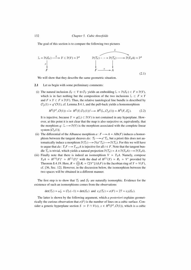
132 Chapter 5. Cubic threefolds
The goal of this section is to compare the following two pictures
L = P(SF)
p
q // Y ⊂ P(V) ' P4
F
P(TF)
q
''
// P(TA)
// P(T0A) ' P4
F a // A(2.1)
We will show that they describe the same geometric situation.
2.1 Let us begin with some preliminary comments:
(i) The natural inclusion SF ⊂ V ⊗ OF yields an embedding L ' P(SF) ⊂ F × P(V),which is in fact nothing but the composition of the two inclusions L ⊂ F × Yand F × Y ⊂ F × P(V). Thus, the relative tautological line bundle is described byOp(1) ' q∗O(1), cf. Lemma 3.4.1, and the pull-back yields a homomorphism
H0(P4,O(1)) ∼− // H0(Y,OY (1))
// H0(L,Op(1)) ' H0(F,S∗F). (2.2)
It is injective, because Y = q(L) ⊂ P(V) is not contained in any hyperplane. How-ever, at this point it is not clear that the map is also surjective or, equivalently, thatthe morphism q : L // P(V) is the morphism associated with the complete linearsystem |Op(1)|.
(ii) The differential of the Albanese morphism a : F // A = Alb(F) induces a homor-phism between the tangent sheaves da : TF // a∗TA, but a priori this does not au-tomatically induce a morphism P(TF) // P(a∗TA) // P(TA). For this we will haveto argue that da : TtF // Ta(t)A is injective for all t ∈ F. Note that the tangent bun-dle TA is trivial, which yields a natural projection P(TA) ' A × P(T0A) // P(T0A).
(iii) Finally note that there is indeed an isomorphism V ' T0A. Namely, composeT0A ' H1,0(F)∗ ' H2,1(Y)∗ with the dual of H2,1(Y) ' R1 ' V∗ provided byTheorem 1.4.19. Here, R =
⊕Ri ' C[V∗]/(∂iF) is the Jacobian ring of Y = V(F),
cf. [36, Sec. 12]. However, in the discussion below, the isomorphism between thetwo spaces will be obtained in a different manner.
The first step is to show that TF and SF are naturally isomorphic. Evidence for theexistence of such an isomorphisms comes from the observations
det(TF) ' ω∗F ' OF(−1) ' det(SF) and c2(TF) = e(F) = 27 = c2(SF).
The latter is shown by the following argument, which a posteriori explains geomet-rically the curious observation that e(F) is the number of lines on a cubic surface. Con-sider a generic hyperplane section S B Y ∩ V(s), s ∈ H0(P4,O(1)), which is a cubic
2 Albanese of the Fano surface 133
surface S ⊂ V(s) ' P3. Let sF be the image of s under H0(P(V),O(1)) // H0(F,S∗F).Its zero set V(sF) ⊂ F is the set of lines [L] ∈ F with s|L = 0, i.e. the set of all linescontained in the cubic surface S .
Proposition 2.1. Let Y ⊂ P4 be a smooth cubic threefold and F = F(Y) its Fano varietyof lines. Then there exists a natural isomorphism
TF ' SF
between the tangent bundle TF of F and the restriction SF of the universal subbundleS ⊂ V ⊗OG under the natural embedding F ⊂ G(1,P4).
Proof The result was originally proved in [36, 150] by very clever geometric argu-ments. We follow the more algebraic approach in [4].
Recall that F ⊂ G = G(1,P4) is the zero set of the regular regular section sY ∈
H0(G, S 3(S∗)). The latter is the image of the equation in S 3(V∗) defining Y under thenatural surjection S 3(V∗) // // S 3(S∗), see Section 3.1.1. Hence, the normal bundle se-quence has the form
0 // TF // TG|F // S 3(S∗F) // 0. (2.3)
Deformation theory, see Section 3.1.2, provides us with descriptions of the fibres of thetwo tangent bundles:
T[L]F ' H0(L,NL/Y ) and T[L]G ' H0(L,NL/P).
Moreover, fibrewise (2.3) is described as the cohomology sequence of the exact se-quence 0 //NL/Y //NL/P //OL(3) // 0 of normal bundles for the nested inclusionL ⊂ Y ⊂ P4. The global version of the latter is the exact sequence of normal bundles ofthe nested inclusion L ⊂ F × Y ⊂ F × P:
0 // NL/F×Y // NL/F×P // NF×Y/F×P|L // 0.
' p∗QF ⊗Op(1) ' q∗O(3) ' Op(3)
(2.4)
We use NLG/G×P ' p∗Q⊗Op(1), which is the global version of the natural isomorphismNL/P ' V/W⊗O(1) for a line L = P(W) ⊂ P(V), cf. the discussion in Section 3.1.2. Here,Q is the universal quotient bundle onG. Restriction to F yields NL/F×P ' p∗QF⊗Op(1).Taking the direct image of (2.4) under p : L // F gives back (2.3):
0 // p∗NL/F×Y // p∗NL/F×P // p∗Op(3) // 0.
' TF ' TG|F ' S 3(S∗F)
(2.5)
The key to describing TF is to view it as the direct image of N B NL/F×Y . Takingdeterminants of (2.4) shows∧2 N ' det(N ) ' det
(p∗QF ⊗Op(1)
)⊗Op(−3) ' p∗ det(QF).

134 Chapter 5. Cubic threefolds
On the other hand, applying∧2 and ⊗Op(−3) to (2.4) yields the exact sequence
0 // ∧2N ⊗Op(−3) // p∗∧2QF ⊗Op(−1) // N // 0.
As p∗Op(−1) ' 0 ' R1 p∗Op(−1), taking direct images gives
TF ' p∗N ' R1 p∗(∧2N ⊗Op(−3)) ' det(QF) ⊗ R1 p∗Op(−3).
By relative Serre duality, cf. [80, III. Ex. 8.4], R1 p∗Op(−3) ' p∗(Op(1))∗ ⊗det(SF) and,therefore, TF ' p∗N ' det(QF) ⊗ SF ⊗ det(SF) ' SF .
Note that SF is naturally viewed as a subbundle SF ⊂ V ⊗OF and, as we will see, TF
as a subbundle TF ⊂ a∗TA ' T0A⊗OF . However, the above result does not yet show thatthere exists an isomorphism SF ' TF that would be compatible with those inclusionsafter choosing an appropriate isomorphism V ' T0A.
Corollary 2.2. The natural map in (2.2) is an isomorphism
V∗ ∼− // H0(F,S∗F).
Hence, q : L // // Y ⊂ P(V) is the morphism associated with the complete linear system|Op(1)|.
Proof Use dim H0(F,S∗F) = dim H0(F, T ∗F ) = dim H1(F,OF) = 5.
2.2 So far, we have shown that there exists an isomorphism L ' P(SF) ' P(TF), butnot that the two morphisms in (2.1) are related. In fact, we have not yet even properlydefined the morphism P(TF) // P(T0A). This will be done next.
The first step towards it will be to show that exterior product yields an isomorphism∧2 H1(F,Q) ∼− // H2(F,Q) of Hodge structures. Due to Section 3.3.3 we in fact know
already that the two Hodge structures are isomorphic
∧2 H1(F,Q) '∧2 H3(Y,Q)(2) ' H2(F,Q),
but not that this isomorphism is given by exterior product.
Lemma 2.3. The exterior product defines isomorphisms
∧2 H1,0(F) ∼ // H2,0(F) and∧2 H1(F,Q) ∼ // H2(F,Q).
Proof Using the isomorphism SF ' TF , the Hodge theoretic assertion is turned into

2 Albanese of the Fano surface 135
the geometric assertion that the natural map∧2 H0(F,S∗F) // H0(F,
∧2 S∗F) is an iso-morphism. Using the commutative diagram∧2 V∗
o
∼ // ∧2 H0(F,S∗F)
H0(P(
∧2 V),O(1)) // H0(F,∧2 S∗F) ' H0(F,OF(1))
and the fact that all spaces are of the same dimension ten, it suffices to show that thePlücker embedding F ⊂ P(
∧2 V) is not contained in any hyperplane. This can eitherbe argued geometrically [36, Lem. 10.2] or using the Koszul complex as in Proposition3.2.3.
As the map∧2 H1(F,Q) // H2(F,Q) is topologically defined, its injectivity is inde-
pendent of the smooth cubic threefold. It is thus enough to check it for one F = F(Y).However, for the very general cubic
∧2 H3(Y,Q)(2) '∧2 H1(F,Q) is the direct sum
Q(−1) ⊕ H of two irreducible Hodge structures of weight two. This can be seen, for ex-ample, as a consequence of the monodromy description Theorem 1.2.9, see Section 0.2and Remark 3.??. The first summand is pure and spanned by the intersection product onH3(Y,Q). It is mapped onto the line spanned by the Plücker polarization g, see Proposi-tion 3.4.2. Due to the irreducibility of the Hodge structure H, the map H // H2(F,Q) isinjective if and only if
∧2 H1,0(F) // H2,0(F) is non-trivial, which we have shown al-ready. Moreover, H2,0(F) is contained in H2(F,C)pr and, therefore, H
// H2(F,Q)pr.Altogether, this proves the injectivity of
∧2 H1(F,Q) // H2(F,Q) and, due to dimen-sion reasons, its bijectivity.
Geometrically, the first injectivity is equivalent to saying that the image of the Al-banese morphism a : F // A is a surface.
Corollary 2.4. The Albanese morphism a : F // A is unramified, i.e. for all t ∈ F thetangent map dat : TtF // Ta(t)A is injective. In particular, the Albanese map defines themorphism q in (2.1)
q : P(TF) // P(TA) // P(T0A).
Proof Assume dat is not injective for some t ∈ F. Then the induced map∧2 TtF // ∧2 Ta(t)A
is trivial. However, this map is dual to the map∧2 T ∗a(t)A '∧2 H1,0(A) '
∧2 H1,0(F) ∼ // H2,0(F) ' H0(F, ωF) // ωF ⊗ k(t),
which then is also trivial. As ωF is very ample and, in particular, globally generated,this is absurd.

136 Chapter 5. Cubic threefolds
Lemma 2.5. The morphism q : P(TF) // P(T0A) is the morphism associated with thecomplete linear system |Op(1)|
Proof First, q∗O(1) ' Op(1), as P(TF) ⊂ P(a∗T0) ' P(T0A) × A is induced by theinclusion TF
// TA ' T0A⊗OF . It remains to show that the linear system is complete,i.e. that the pull-back map H0(P(T0A),O(1)) // H0(P(TF),Op(1)) is a bijection. Bothsides are of dimension five, so it suffices to prove the injectivity. If the map were notinjective, then all tangent spaces TtF
// T0A would be contained in a hyperplane. Butthis would contradict the bijectivity of the dual map H0(A,ΩA) // H0(F,ΩF), which isthe pull-back of one-forms under the Albanese map a : F // A.
This proves the main result of this section:
Proposition 2.6. There exist isomorphisms SF ' TF and V ' T0A inducing a commu-tative diagram
P(SF)
o
q // P(V)
o
P(TF)
q// P(T0A)
Corollary 2.7. The Albanese morphism a : F // A is unramified and generically in-jective.
Proof The first assertion is Corollary 2.4. To prove the injectivity generically, wechoose the above isomorphism V ' T0A such that the two inclusions
TF // a∗TA ' T0A ⊗OF and SF
// V ⊗OF
coincide. Hence, the morphism F //G(1,P(T0A)), t // [TtF ⊂ T0(A)] is identifiedwith the Plücker embedding F
// G(1,P(V)). However, if for all points s ∈ a(F) anddistinct points t1 , t2 ∈ a−1(s) the tangent spaces Tt1 F ⊂ T0A and Tt2 F ⊂ T0A aredifferent, then the generic fibre consists of just one point.
In fact, it has been shown by Beauville that a B F // A is injective and hence
a closed immersion [11, Thm. 4], see Corollary 3.4. We will see that this assertion isequivalent to saying that the invertible sheaves O(CL1 ) and O(CL2 ) associated with twodistinct lines L1 , L2 ⊂ Y are never isomorphic.
2.3 The following is a special case of the ‘geometric global Torelli theorem’, seeProposition 3.2.8. The result in dimension three [36] predates the general result and theproof is different.

3 Albanese, Picard, and Prym 137
Proposition 2.8. Two smooth cubic threefolds Y,Y ′ ⊂ P4 are isomorphic if and only iftheir Fano surfaces F(Y) and F(Y ′) are isomorphic:
Y ' Y ′ ⇔ F(Y) ' F(Y ′).
Proof For any smooth cubic threefold Y ⊂ P4, the Picard group Pic(Y) is gener-ated by OY (1). Hence, any isomorphism Y ' Y ′ is induced by an automorphism ofthe ambient P4 and, therefore, induces an isomorphism F(Y) ' F(Y ′) between theirFano surfaces. Conversely, any isomorphism F(Y) ' F(Y ′) induces an isomorphismY ' Y ′ between the images of the natural morphisms P(TF(Y)) // P(T0Alb(F(Y))) andP(TF(Y ′)) // P(T0Alb(F(Y ′))), given by the differentials of the Albanese maps.
Exercise 2.9. The same techniques show that for any smooth cubic threefold Y ⊂ P4
there exists a natural isomorphism of finite groups (cf. Corollary 1.3.6)
Aut(Y) ' Aut(F(Y)).
Quotients of F(Y) by subgroups of Aut(F(Y)) have been studied in [137].
We complement this result by the following infinitesimal statement which moreovershows that the Fano surface F(Y) stays a Fano surface after deformation, which is falsefor example for the Fano variety of lines on a smooth cubic fourfold, see Section ??.??.
Proposition 2.10. Let Y ⊂ P4 be a smooth cubic threefold and let F = F(Y) be its Fanosurface. Then the natural map
H1(Y, TY ) // H1(F, TF)
is an isomorphism.
Proof
3 Albanese, Picard, and Prym
The general theory set up in Section 3.4.2 provides us with a commutative diagram
CH2(F)alg
// CH2(Y)alg
// CH1(F)alg
o
A(F) // // J(Y) // // Pic0(F).
Note that CH2(F)alg is known to be big (over C), while CH1(F) ' Pic(F).The intermediate Jacobian J(Y) B J3(Y) of Y is self-dual and the two maps on the
bottom are dual to each other, cf. Section 3.4.2. Indeed, they are induced by the Fano

138 Chapter 5. Cubic threefolds
correspondence ϕ : H3(Y,Z) // H1(F,Z)(−1) and its dual ψ : H3(F,Z) // H3(Y,Z) (upto torsion, see Remark 3.9). Moreover, as the two maps induce isomorphisms betweenthe cohomology groups with rational coefficients, they are isogenies of abelian varietiesof dimension five.
The aim of this section is to show that all three abelian varieties are isomorphic and,moreover, can be identified with the Prym variety of the morphism CL ' DL // DL inSection 1.3.
3.1 In order to understand the composition A = A(F) // // J(Y) // // Pic0(F), wecompose it with the Albanese map a : F // A, which depends on the additional choiceof a point t0 = [L0] ∈ F and factorizes via F //CH2(F)alg, t // [t]−[t0] and the Abel–Jacobi map CH2(F)alg ⊂ CH2(F)hom // A(F). Note that eventually Corollary 3.10 willimply that
CH2(Y)alg = CH2(Y)hom and Pic0(F) ' CH1(F)alg = CH1(F)hom.
The latter is equivalent to Pic(F)/Pic0(F) being torsion free or, still equivalently, toH2(F,Z) being torsion free.
Lemma 3.1. The composition F // A(F) // // J(Y) // // Pic0(F) sends [L] ∈F to the invertible sheaf O(CL −CL0 ).
Proof Clearly, the class of the point t = [L] ∈ F under ϕ : CH2(F) //CH2(Y) ismapped to the class [L] ∈ CH2(Y) of the line L ⊂ Y . The image of the latter under thecorrespondence ψ : CH2(Y) //CH1(F) is by construction O(CL).
The result can be extended to yield for every (smooth) curve C ⊂ F a description ofthe composition
C // A(C) // A(F) // // J(Y) // // Pic0(F) // Pic0(C),
as [L] //O(CL − CL0 )|C . This is particularly useful when C is ample, e.g. C = CL. Inthis case,
A(C) // // A(F) and Pic0(F) // Pic0(C),
as by Kodaira vanishing theorem H1(F,OF) // H1(C,OC) is injective.Let [L] ∈ F be generic and consider CL as the étale cover
π : CL ' DL // // DL
of degree two, see Section 1.3.
Corollary 3.2. The composition
Pic0(DL) π∗ // Pic0(CL) ' A(CL) // // A(F) // // J(Y) // // Pic0(F)

3 Albanese, Picard, and Prym 139
is trivial. Dually, the image of the restriction map H1(F,Z) // H1(CL,Z) is containedin the kernel of π∗ : H1(CL,Z) // H1(DL,Z).
Proof Observe that under the natural map
DL // Pic(DL) // Pic(CL) //CH2(F) //CH2(Y)
a point y ∈ DL is mapped to [L1] + [L2] ∈ CH2(Y), where L1 and L2 correspond to thetwo points of the fibre π−1(y). Clearly, [L1]+ [L2] = [L1]+ [L2]+ [L]− [L] = [P2]|Y − [L],where P2 = y L. As [y L] ∈ CH2(P4) ' Z is independent of y ∈ DL, the class [L1]+[L2] ∈CH2(Y) is independent of y and, therefore, DL //CH2(Y) //CH1(F) is constant.
By a purely topological description of étale coverings of degree two, one computesthat the intersection pairing on H1(CL,Z) restricted to
H1(CL,Z)− B Ker(π∗ : H1(CL,Z) // H1(DL,Z)
)is divisible by two, cf. Section 3.2. Hence, the Hodge–Riemann pairing ( . )F on H1(F,Z)with respect to the Plücker polarization is of the form
(γ.γ′)F =
∫Fγ · γ′ · g = 3
∫CL
γ|CL · γ′|CL ∈ 6Z,
where we use Lemma 1.11 showing that 3 [CL] = g ∈ H2(F,Z). Then, according toProposition 3.4.2, the Fano correspondence yields an injection of integral(!) symplecticlattices
ϕ : (H3(Y,Z), ( . )Y ) // (H1(F,Z), (−1/6)( . )F)
of finite index. As the left hand side is unimodular, it has to be an isomorphism. We thushave proved the following result.
Corollary 3.3. The Fano correspondence induces an isomorphism of Hodge structures
ϕ : H3(Y,Z) ∼− // H1(F,Z)(−1)
and the induced morphisms between the associated abelian varieties are isomorphisms
A(F) ∼− // J(Y) ∼
− // Pic0(F).
The next result improves Corollary 2.7.
Corollary 3.4. The Albanese morphism
a : F // A(F)
is a closed immersion. Equivalently, the natural morphism F // Pic(F), [L] //O(CL)
is a closed immersion
140 Chapter 5. Cubic threefolds
Proof Indeed, due to Corollary 2.7 the morphism F // A(F) is unramified and itscomposition with the A(F) // J(Y) // Pic(F), which is an isomorphism by Corollary3.3, is the injective map [L] //O(CL), cf. Corollary 1.22.
3.2 The next aim is to relate the intermediate Jacobian J(Y) to the Prym variety ofthe étale cover CL // // DL for any generic line L ⊂ Y . Let us begin with a reminderon Prym varieties. See [9, 107, 122] for a detailed discussion and [64] for a historicalaccount.
We consider an étale cover π : C // // D of degree two between smooth projectivecurves. Its corresponding two-torsion line bundle Lπ ' π∗OC/OD ∈ Pic0(D) satisfiesπ∗Lπ ' OC . We shall denote the covering involution by ι and its natural action on thePicard variety by ι∗ : Pic(C) // Pic(C).
Lemma 3.5. The pull-back π∗ : Pic(D) // Pic(C) yields an isomorphism
Pic(D)/〈Lπ〉 ' Ker ( Pic(C) 1−ι∗ // Pic(C) ).
Proof The morphism 1 − ι∗ maps a line bundle L to L ⊗ ι∗L∗. Clearly, if L = π∗M,then (1 − ι∗)(L) ' OC . For the other inclusion use that any ι∗-invariant invertible sheafdescends to an invertible sheaf on D.1 Following [9], the descent can be shown explicitlyas follows: Suppose L = O(E) satisfies ι∗L ' L. Write L⊗ ι∗L∗ as the principal divisor( f ) for some f ∈ K(C) and observe that then f · ι∗ f has neither zeros nor poles, so wemay assume f · ι∗ f = 1 (we need k to admit square roots for this). Pick an elementg ∈ K(C) with ι∗g = −g and set f0 B g · ( f − 1). Then, f = f0 · (ι∗ f0)−1 and, therefore,E0 B E − ( f0) is the pull-back of a divisor on D. We leave it to the reader to verify thatOD and Lπ are the only line bundles with trivial pull-back to C.
Definition 3.6. The Prym variety of an étale cover π : C // // D of degree two is definedas
Prym (C/D) B Im ( Pic0(C) 1−ι∗ // Pic(C) ).
Hence, there exists a natural exact sequence [22, Thm. 2], [9, Sec. 2.6], [126, Sec.10.9]
0 // 〈Lπ〉 // Pic0(D) // Pic0(C) // Prym(C/D) // 0. (3.1)
Alternatively, the Prym variety can be viewed as a connected component of the kernelof the norm map. Recall that the norm map N : Pic(C) // Pic(D) is the push-forwardmap π∗ : CH1(C) //CH1(D) or, on the identity component and using Pic0 ' Albfor curves, the natural map Alb(C) //Alb(D). It can also be described as N(L) '
1 One could think that the absence of fixed points is important here. It is not, although for the descent ofinvariant invertible sheaves on surfaces, fixed points do cause problems.

3 Albanese, Picard, and Prym 141
det π∗L ⊗ (det π∗OC)∗. For example, for the line bundle L = O(x), x ∈ C, the exact se-quence 0 //OC //L // k(x) // 0 indeed yields O(π(x)) ' det π∗k(x) ' det π∗L ⊗(det π∗OC)∗. Clearly, N defined as π∗ is a group homomorphism, which is not quite soapparent in the latter description. Then
Prym (C/D) = Im (1 − ι∗) ' Ker (N)o
is the connected component of the kernel containing OC . In fact, Ker(N) has exactlytwo connected components Ker(N) = PrymtPrym′, non-canonically isomorphic toeach other. For one inclusion use π∗ι∗ = π∗ and compute N(L ⊗ ι∗L∗) ' det π∗(L) ⊗(det π∗ι∗L)∗ ' OD. For the other, observe that N : Pic0(C) // // Pic0(D) is surjective andhence Prym (C/D) ⊂ Ker (N)o is an inclusion of abelian varieties of the same dimen-sion.
To summarize, in addition to the exact sequence (3.1) there is an exact sequence
0 // Prym t Prym′ // Pic0(C) N // Pic0(D) // 0.
' A(C) ' A(D)
(3.2)
It may be helpful to describe both points of view in terms of integral Hodge structures.Recall that
Pic0(C) 'H1(C,OC)H1(C,Z)
'H0(C, ωC)∗
H1(C,Z)
and similarly for Pic0(D). As explained in [107, Ch. 12.4], H1(C,Z) admits a symplecticbasis of the form λ0, µ0, λ
±i , µ
±i , i = 1, . . . , g(D) − 1 with λ0, µ0 fixed by the action of ι∗
on H1(C,Z) and ι∗(λ±i ) = λ∓i , ι∗(µ±i ) = µ∓i . This allows one to describe the eigenspacesH1(C,Z)± ⊂ H1(C,Z) of the involution ι∗ as
H1(C,Z)+ = 〈λ0, µ0, λ+i + λ−i , µ
+i + µ−i 〉 and H1(C,Z)− = 〈λ+
i − λ−i , µ
+i − µ
−i 〉.
The latter implies the fact alluded to before that the intersection pairing on H1(C,Z)−
is divisible by 2, which was used in the proof of Corollary 3.3. Moreover, the image ofthe pull-back map
π∗ : H1(D,Z) = 〈λi, µi〉i=0,...,g(D)−1 // H1(C,Z)+,
which is given by λ0 // λ0, µ0
// 2 µ0, λi // λ+
i + λ−i , and µi // µ+
i + µ−i , for i =
1, . . . , g(D) − 1, yields a sublattice of index two. With this notation, topologically theétale covering C // D can be constructed by cutting D along the standard loop repre-senting µ0 and glueing two copies of D along µ0. This explains why in particular thepull-back of µ0 yields 2 µ0.
Also observe that the image of
H1(C,Z) // H1(C,Z)+, α // α + ι∗α

142 Chapter 5. Cubic threefolds
is contained in π∗H1(D,Z) ⊂ H1(C,Z)+ with index two. On the other hand,
H1(C,Z) // // H1(C,Z)−, α // α − ι∗α
is surjective. The sequence (3.1) is induced by the exact sequence
0 // H1(C,Z)+ // H1(C,Z) 1−ι∗ // H1(C,Z)− // 0, (3.3)
which allows one to describe the Prym variety as
Prym(C/D) 'H1(C,OC)−
H1(C,Z)−'
H0(C, ωC)−∗
H1(C,Z)−.
Remark 3.7. The Prym variety is commonly viewed as a principally polarized abelianvariety: Indeed, the last isomorphism together with the description of H1(C,Z)− as 〈λ+
i −
λ−i , µ+i − µ
−i 〉 allows one to define a principal polarization on Prym(C/D) explicitly as
given by the intersection pairing on H1(C,Z)− up to the factor (1/2).
The kernel of Pic0(C) // // Prym(C/D) can be written as the degree two quotient
Pic0(D) 'H1(C,OC)+
H1(D,Z)// // H
1(C,OC)+
H1(C,Z)+.
On the other hand, the sequence (3.2) corresponds to
0 // H1(C,Z)− // H1(C,Z) 1+ι∗ // (1 + ι∗)H1(C,Z) // 0,
using the degree two quotient
H1(C,OC)+
(1 + ι∗)H1(C,Z)// // H
1(C,OC)+
H1(D,Z)' Pic0(D).
Let us now apply this to the cover CL // // DL associated with any generic line L ⊂ Y .
Proposition 3.8 (Mumford). For a generic line L ⊂ Y, the inclusion i : CL // F(Y)
induces an isomorphism
Prym(CL/DL) ∼− // A(F) ' J(Y) ' Pic0(F).
Proof The assertion follows from a comparison of (3.3) with the exact sequence
0 // Ker(ξ) // H1(CL,Z)ξ // H3(Y,Z) // 0.
Here, ξ is the composition of the push-forward map i∗ : H1(CL,Z) // H3(F(Y),Z) viathe closed embedding i : CL
// F(Y) and of the dual ψ : H3(F(Y),Z) // // H3(Y,Z) ofthe Fano correspondence. The surjectivity of i∗ is a consequence of the ampleness ofCL and the Lefschetz hyperplane theorem H1(CL,Z) ' H1(CL,Z) // // H1(F(Y),Z) 'H3(F(Y),Z). As ψ is (up to torsion) dual to ϕ : H3(Y,Z) ∼
− // H1(F(Y),Z), which is anisomorphism according to Corollary 3.3, ψ is surjective, too.

3 Albanese, Picard, and Prym 143
Due to Corollaries 3.2 and 3.3, we know that H1(DL,Z) // H3(F(Y),Z) is trivialand, hence, H1(DL,Z) ⊂ Ker(ξ). Both are free Z-modules of the same rank and Ker(ξ)is saturated, as its cokernel is the torsion free H3(Y,Z). On the other hand, H1(DL,Z)is also contained with finite index in H1(CL,Z)+, which is a saturated submodule ofH1(CL,Z) (its cokernel is the torsion free H1(CL,Z)−). Hence, Ker(ξ) and H1(CL,Z)+
both realize the saturation of H1(DL,Z) ⊂ H1(CL,Z) and, therefore, coincide. But thenthere is an isomorphism of Hodge structures (up to Tate twist) H3(Y,Z) ' H1(CL,Z)−
and, hence, Prym(CL/DL) ' J(Y).
Remark 3.9. There is a subtlety that has been avoided in the above discussion: Isψ : H3(F(Y),Z) // // H3(Y,Z) an isomorphism? This is true up to torsion in H3(F(Y),Z),which in any case does not effect the isomorphism J(Y) ' A(F). Nevertheless, it wouldbe interesting to decide whether there is non-trivial torsion in H3(F(Y),Z) or, similarly,in H2(F(Y),Z). The torsion freeness of the latter would in particular prove that numeri-cal equals algebraic equivalence for line bundles on F(Y), see below.
As a consequence, one obtains a description of the algebraically trivial part of theChow group of curves on Y .
Corollary 3.10. For a generic line L ⊂ Y (in the sense of Corollary 1.8) the Abel–Jacobimap yields an isomorphism of groups
CH2(Y)alg∼− // J(Y) ' Prym(CL/DL).
Proof The result can be seen as an application of a result of Bloch and Srinivas [21,Thm. 1]: If Y is a smooth complex projective variety with CH0(Y) ' Z, then the Abel–Jacobi map induces isomorphisms of groups
CH2(Y)alg ' CH2(Y)hom∼− // J(Y). (3.4)
Clearly, as on a cubic threefold any two points can be connected by a chain of lines,cubic threefolds satisfy the assumption.
However, in our case of a smooth cubic threefold more direct arguments for the iso-morphism CH2(Y)alg ' J(Y) exist, see [125, 126, 127] or [9, Thm. 3.1].
Remark 3.11. The arguments in the above discussion heavily rely on the ground fieldbeingC. In fact, already the definition of the intermediate Jacobian J(Y) over other fieldsis problematic. However, CH2(Y) and Prym(CL/DL) make perfect sense over arbitraryfields. And, indeed, Murre in [125] describes an algebraic approach that yields an iso-morphism CH2(Y)alg ' Prym(CL/DL) over arbitrary algebraically closed fields. In fact,the isomorphism was originally stated up to elements of order two, but the divisibilityof CH2(Y)alg (pointed out by Bloch, see the review of [125]), yields the full statement.
Remark 3.12. In [36, App. A] one finds a geometric argument that shows a weaker ver-sion of the first isomorphism in (3.4), namely that the difference between CH2(Y)hom and

144 Chapter 5. Cubic threefolds
CH2(Y)alg is annihilated by 6. More precisely, it is shown that 6 CH2(Y)hom = CH2(Y)alg.The idea is the following: Let C ⊂ Y be any curve. Then a surface C ⊂ S ⊂ Y is con-structed such that 6 C on S is rationally equivalent to the sum of nH|S and a sum of lines∑
aiLi. As Pic(Y) ' Z, this proves the assertion. The surface S is obtained as the imageq(S ) of the surface S B p−1(p(q−1(C))) parametrizing pairs (L, x) consisting of a pointx contained in the line L that intersects C. Clearly, S is a P1-bundle over p(q−1(C)),which comes with a natural section q−1(C) ⊂ S . Its image under q∗ yields 6 C.
4 Global Torelli theorem and irrationality

6
Cubic fourfolds
1 Lattice and Hodge theory for cubic fourfolds and K3 surfaces
In the first section, we collect all facts from Hodge and lattice theory relevant for thestudy of cubic fourfolds. The curious relation between the lattice theory of cubic four-folds and K3 surfaces has been systematically studied first by Hassett [82]. Earlier re-sults in this direction are due to Beauville and Donagi [16]. 1
1.1 As we have seen in Section ??.??, as abstract lattices the middle cohomologyand the primitive cohomology of a smooth cubic fourfold X ⊂ P5 are described by
H4(X,Z) ' I21,2 ' E⊕28 ⊕ U⊕2 ⊕ I3,0,
H4(X,Z)pr ' E⊕28 ⊕ U⊕2 ⊕ A2,
where h2 = (1, 1, 1) ∈ I3,0. It will be convenient to change the sign and introduce thecubic lattice and the primitive cubic lattice as
Γ B I2,21 ' E8(−1)⊕2 ⊕ U⊕2 ⊕ I0,3 ' H4(X,Z)(−1),
Γ B E8(−1)⊕2 ⊕ U⊕2 ⊕ A2(−1) ' H4(X,Z)pr(−1).
In particular, from now on (h2)2 = −3. The twist should not be confused with the Tatetwist of the Hodge structure. It turns out that E8(−1)⊕2, certainly the most interestingpart of these lattices, will hardly play any role in our discussion. We shall henceforthabbreviate it by
E B E8(−1)⊕2
and consequently write
Γ ' E ⊕ U⊕2 ⊕ I0,3 and Γ ' E ⊕ U⊕2 ⊕ A2(−1).
Version Oct 19, 2018. The first two sections are still in very rough form. Feedback will be most welcome.1 This part is based on lectures given at the school ‘Birational Geometry of Hypersurfaces’ in Gargnano in
March 2018.
145

146 Chapter 6. Cubic fourfolds
In the discussion below, the intersection form of a K3 surface will be central, althoughthere is a priori no geometric reason why K3 surfaces should enter the picture at all. Ina first step, we shall deal with this purely on the level of abstract lattice theory and lateradd Hodge structures.
Recall that for a complex K3 surface S , its middle cohomology with the intersectionform is the lattice
H2(S ,Z) ' E ⊕ U⊕3 ' E ⊕ U1 ⊕ U2 ⊕ U3 C Λ,
see [90, Ch. 14]. The summands Ui, i = 1, 2, 3, are copies of the hyperbolic planeU. Indexing them will make the discussion more explicit and will help us to avoidambiguities later on.
The full cohomology H∗(S ,Z) is also endowed with a unimodular intersection form.It is customary to introduce a sign in the pairing on (H0 ⊕ H4)(S ,Z), which, however,does not change the abstract isomorphism type, for U ' U(−1). The resulting lattice isthe Mukai lattice
H(S ,Z) B H2(S ,Z) ⊕ (H0 ⊕ H4)(S ,Z) ' E ⊕ U⊕3 ⊕ U4
' E ⊕ U1 ⊕ U2 ⊕ U3 ⊕ U4 C Λ.
The standard basis of U consists of isotropic vectors e, f with (e. f ) = 1. We shall denotethe standard bases in the first three copies of U as ei, fi ∈ Ui, i = 1, 2, 3. However,in order to take into account the sign change in the Mukai pairing, we shall use theconvention that (e4. f4) = −1 and that e4 = [S ] ∈ H0(S ,Z) and f4 = [x] ∈ H4(S ,Z).
Next, we introduce an explicit embedding A2 // Λ. Here, A2 = Z λ1 ⊕ Z λ2 is the
lattice of rank two given by the intersection form(
2 −1−1 2
)and we define
A2 // U3 ⊕ U4 ⊂ Λ (1.1)
by λ1 // e4− f4 and λ2
// e3+ f3+ f4. The orthogonal complement 〈λ1, λ2〉⊥ = A⊥2 ⊂ Λ
is the lattice
A⊥2 = E ⊕ U1 ⊕ U2 ⊕ A2(−1),
where A2(−1) ⊂ U3 ⊕U4 is spanned by µ1 B e3 − f3 and µ2 B −e3 − e4 − f4 satisfying(µi)2 = −2 and (µ1.µ2) = 1.
Remark 1.1. We observe that λ⊥1 = E ⊕ U1 ⊕ U2 ⊕ U3 ⊕ Z(−2), where the last directsummand is generated by e4 + f4. Hence, λ⊥1 ' Λ ⊕ Z(−2). As H2(S ,Z) ' Λ andH2(S [2],Z) ' H2(S ,Z) ⊕ Z(−2) for the Hilbert scheme S [2] of any K3 surface S , thiscan be read as a lattice isomorphism λ⊥1 ' H2(S [2],Z).

1 Lattice and Hodge theory for cubic fourfolds and K3 surfaces 147
The discussion so far leads to the fundamental observation that there exists an iso-morphism
Γ ⊃ Γ ' A⊥2 ⊂ Λ
between the primitive cubic lattice Γ and the lattice A⊥2 inside the Mukai lattice Λ.For later use, we record that (1.1) induces inclusions of index three:
A2 ⊕ A2(−1) ⊂ U3 ⊕ U4 and A2 ⊕ A⊥2 ⊂ Λ,
where, for example, the quotient of the latter is generated by the image of the class(1/3)(µ1 − µ2 − λ1 + λ2) = e3 + f4.
Another technical result that will be crucial at some point later, is the following ele-mentary statement which is surprisingly difficult to prove, cf. [3, Prop. 3.2].
Lemma 1.2. Consider A2 ⊂ Λ as before, let U // Λ be an isometric embedding of a
copy of the hyperbolic plane, and denote by A2 + U the saturation of A2 + U ⊂ Λ. Thenthere exists an isometric embedding of a copy of the hyperbolic plane U′
// A2 + Usuch that rk(A2 + U′) = 3.
Proof Clearly, if rk(A2 + U) = 3, there is nothing to prove, so we can restrict to thecase that the rank is four.
Remark 1.3. To motivate the notion of Noether–Lefschetz (or Heegner) divisors forcubic fourfolds, let us recall the corresponding concept for K3 surfaces: For a primitiveclass ` ∈ Λ with (`)2 = d, we write
Λd B `⊥ ⊂ Λ.
As ` is in the same O(Λ)-orbit as the class e2 + (d/2) f2, cf. [90, Cor. 14.1.10], it canabstractly be described as
Λd ' E ⊕ U⊕2 ⊕ Z(−d).
It is important to note that the lattices Λd are in general not contained in A⊥2 ⊂ Λ.
We shall call any primitive vector v ∈ Γ ' A⊥2 with (v)2 < 0 a Noether–Lefschetzvector. With such Noether–Lefschetz vector one naturally associates two lattices. Onthe cubic side, one defines
Z h2 ⊕ Z v ⊂ Kv ⊂ Γ
as the saturation of Z h2 ⊕ Z v ⊂ Γ. On the K3 side, we introduce the saturation
A2 ⊕ Z v ⊂ Lv ⊂ Λ.
Note that Lv is of rank three and signature (2, 1), while Kv is of rank two and signature(0, 2). Clearly, their respective orthogonal complements are isomorphic:
Γ ⊃ K⊥v ' L⊥v ⊂ Λ,

148 Chapter 6. Cubic fourfolds
as they are both described as v⊥ ⊂ Γ ' A⊥2 . In particular, for the discriminants2 we have
d B disc(Lv) = disc(Kv).
The situation has been studied in depth in [82], where one also finds the next result.
Lemma 1.4 (Hassett). Only the following two cases can occur:
(i) Either Z h2 ⊕ Z v = Kv, A2 ⊕ Z v = Lv, and
d = disc(Kv) = disc(Lv) = −3 (v)2 ≡ 0 (6)
(ii) or Z h2 ⊕ Z v ⊂ Kv, A2 ⊕ Z v ⊂ Lv are both of index three, and
d = disc(Kv) = disc(Lv) = −13
(v)2 ≡ 2 (6).
Proof The main ingredient is the standard formula, see e.g. [90, Sec. 14.0.2],
disc(Kv) · [Kv : Z h2 ⊕ Z v]2 = disc(Z h2 ⊕ Z v) = −3 (v)2.
Any y ∈ Kv is of the form y = s h2 + t v, with s, t ∈ Q. From (h.y) ∈ Z one concludess ∈ (1/3)Z and hence also t ∈ (1/3)Z. This shows that [Kv : Z h2 ⊕ Z v] = 1, 3, or = 9,but the last possibility is excluded as (1/3) h2 < Γ.
In the first case, i.e. Kv = Z h2 ⊕ Z v, one finds d = disc(Kv) = −3 (v)2 ≡ 0 (6). Inthe second case, so when the index is three, then 3 d = −(v)2 ≡ 0, 2, 4 (6). On the otherhand, Kv admits a basis consisting of h2 and another class x. Indeed, pick any classx ∈ Kv whose image generates the quotient Kv/(Z h2 ⊕ Z v) ' Z/3Z. We may assume3 x = s h2 + t v with s, t ∈ ±1 and, therefore, Kv = Z h2 ⊕ Z x. Hence, its discriminantsatisfies d = −3 (x)2 − (x.h2)2 ≡ 0, 2, 3, 5 (6). Altogether this shows that d ≡ 0, 2 (6).
We claim that d ≡ 0 (6) holds if and only if Kv = Z h2 ⊕ Z v. The ‘if’-direction’ wasproved already. For the ‘only if’-direction, assume that d ≡ 0 (6) but [Kv : Z h2 ⊕ Z v] =
3. Pick x ∈ Kv as above. Then, write v = s h2 + t x, s, t ∈ Z, and use (v.h2) = 0 andthe primitivity of v to show v = r ((x.h2) h2 + 3 x) with r = ±1,±(1/3) as v is primitive.However, (x.h2) ≡ 0 (3) under the assumption that d ≡ 0 (6). Hence, ±v = m h2 + x,m ∈ Z, and, therefore, x ∈ Z h2 ⊕ Z v. This yields a contradiction and thus proves theassertion.
The assertions for the lattice Lv follows directly from the ones for Kv.
Remark 1.5. Depending on the perspective, it may be useful to study the various casesfrom the point of view of d or, alternatively, of (v)2. To have the results handy for lateruse, we restate the above discussion as
d ≡ 0 (6) ⇒ (v)2 = −d/3 ≡ 0 (6) or ≡ ±2 (6),d ≡ 2 (6) ⇒ (v)2 = −3 d ≡ 0 (6)
2 The sign of the discriminant will be of no importance in our discussion, we tacitly work with its absolutevalue.

1 Lattice and Hodge theory for cubic fourfolds and K3 surfaces 149
and
(v)2 ≡ ±2 (6) ⇒ d = −3 (v)2 ≡ 0 (6),(v)2 ≡ 0 (6) ⇒ d = −3 (v)2 ≡ 0 (6) or d = −(1/3) (v)2 ≡ 2 (6).
In particular, d determines (v)2 uniquely, but not vice versa unless (v)2 ≡ 2, 4 (6).
Proposition 1.6 (Hassett). Let v, v′ ∈ Γ be two primitive vectors and assume thatdisc(Lv) = disc(Lv′ ) or, equivalently, disc(Kv) = disc(Kv′ ). Then there exist an orthogo-nal transformations g ∈ O(Γ) such that g(v) = ±v′ and, in particular,
Lv′ ' Lg(v) and Kv′ ' Kg(v).
See Section 1.2.4 for the definition of O(Γ), which we also recall below.
Proof One applies Eichler’s criterion, cf. [71, Prop. 3.3]: If an even lattice N is ofthe form N ' N′ ⊕ U⊕2, then a primitive vector v ∈ N with prescribed (v)2 ∈ Z and(1/n) v ∈ AN , with n determined by (v.N) = nZ, is unique up to the action of O(N).Apply this to v ∈ Γ ' A⊥2 ' E ⊕ U⊕2 ⊕ A2(−1) and use that for any primitive v ∈ Γ,either (v.Γ) = Z or = 3Z. This follows from [Γ : Γ ⊕ Z h2] = 3 and the unimodularity ofΓ.
(i) If (v)2 ≡ 0 (6), there are two cases: Assume first that d ≡ 2 (6) or, equivalently, thatZ v⊕Z h2 is not saturated. Then, one finds an element of the form α B (1/3) v+ t h2 ∈ Γ.As (α.w) ∈ Z for all w ∈ Γ, this shows (v.Γ) ⊂ 3Z. Hence, n = 3 and (1/3) v = ±1 ∈AΓ ' Z/3Z.
Assume now that d ≡ 0 (6) and write v = n1v1 + n2v2 with v1 ∈ E ⊕ U1 ⊕ U2 andv2 ∈ A2(−1), both primitive, and n1, n2 ∈ Z. If n1 . 0 (3), then there exists a classw in the unimodular lattice E ⊕ U1 ⊕ U2 ⊂ Γ with (v.w) < 3Z and hence (v.Γ) = Z.If n1 ≡ 0 (3), then n2 . 0 (3), as v is primitive. However, in this case (1/3) (v ± h2) =
(n1/3)v1 +(1/3) (n2v2±h2) ∈ Γ and so Z v⊕Z h2 is not saturated, contradicting d ≡ 0 (6).
(ii) If (v)2 ≡ 2, 4 (6) and hence (v)2 . 0 (3), then (v.Γ) = Z, n = 1, and v ∈ AΓ istrivial.
Hence, in case (i) and (ii), if indeed d and not only (v)2 is fixed, then (v)2 = (v′)2 and(1/n) v = (1/n) v′ ∈ AΓ (up to sign).
Remark 1.7. Due to the uniqueness, no information is lost when explicit classes v ∈Γ ' A⊥2 are chosen for any given d. In the sequel, we will work with the following ones.
(i) For d ≡ 0 (6), one may choose vd B e1 − (d/6) f1 ∈ U1 ⊂ Γ. Observe that indeed,as explained in the general context above, (vd)2 = −d/3 and that the lattice A2 ⊕ Z vd issaturated (use A2 ⊂ U2 ⊕ U3 and vd ∈ U1), i.e.
Ld B Lvd = A2 ⊕ Z vd.

150 Chapter 6. Cubic fourfolds
Similarly,
Kd B Kvd = Z h2 ⊕ Z vd,
which again shows (vd)2 = −d/3. Their orthogonal complement is
Γd B L⊥d ' K⊥d ' E ⊕ U2 ⊕ A2(−1) ⊕ Z (e1 + (d/6) f1)
and their discriminant group
AK⊥d' AKd ' Z/3Z ⊕ Z/(d/3)Z
is cyclic if and only if 9 - d.(ii) For d ≡ 2 (6), one sets vd B 3 (e1 − ((d − 2)/6) f1) + µ1 − µ2 ∈ U1 ⊕ A2(−1). Then
both inclusions
A2 ⊕ Z vd ⊂ Ld B Lvd and Z h2 ⊕ Z vd ⊂ Kd B Kvd
are of index three, for example vd−λ1+λ2 and vd−h2 are divisible by 3. Use λ1 = e4− f4,λ2 = e3 + f3 + f4, µ1 = e3 − f3, and µ2 = −e3 − e4 − f4, the latter corresponding to(1,−1, 0), (0, 1,−1) ∈ Z⊕3. In this case, see [2, 82, 148],
Γd B L⊥d ' K⊥d ' E ⊕ U2 ⊕ (Z⊕3, ( . )A) with A B
−2 1 01 −2 10 1 (d − 2)/3
and Ld and Kd are given by the matrices −A and(
−3 11 −(d + 1)/3
).
The discriminant groups for d ≡ 2 (6) are cyclic, indeed AK⊥d' AKd ' Z/dZ.
In addition to the orthogonal group
O(Γ) B g ∈ O(Γ) | g(h2) = h2 (1.2)
(see Section 1.2.4), which we will also think of as O(Γ) = g ∈ O(Γ) | g ≡ id on AΓ ,we need to consider
O(Γ,Kd) B g ∈ O(Γ) | g(Kd) = Kd, i.e. g(vd) = ±vd ⋃O(Γ, vd) B g ∈ O(Γ) | g|Kd = id, i.e. g(vd) = vd .
Observe that O(Γ, vd) can be identified with the subgroup of all g ∈ O(Γd) with trivialaction on the discriminant AΓd ' AKd . Also, by definition, O(Γ, vd) ⊂ O(Γ,Kd) is asubgroup of index one or two. Note that the natural homomorphism O(Γ,Kd) //O(Kd)is neither surjective (let alone injective) nor is its image contained in O(Kd).

1 Lattice and Hodge theory for cubic fourfolds and K3 surfaces 151
Lemma 1.8 (Hassett). The subgroup O(Γ, vd) ⊂ O(Γ,Kd) is of index at most two. Moreprecisely, one distinguishes the following cases:
(i) If d ≡ 0 (6), then
O(Γ, vd) ⊂ O(Γ,Kd)
has index two.(ii) If d ≡ 2 (6), then
O(Γ, vd) = O(Γ,Kd).
Proof (i) According to Lemma 1.4, d ≡ 0 (6) if and only if Z h2 ⊕ Z vd = Kd, which iscontained in I0,3 ⊕ U1. Let g ∈ O(Γ) be the orthogonal transformation defined by g = idon E ⊕ U2 ⊕ I0,3 and by g = −id on U1. Then g is an element in O(Γ,Kd) \ O(Γ, vd).
(ii) Now, d ≡ 2 (6) if and only if Z h2 ⊕ Z vd ⊂ Kd has index three and then vd =
3 (e1 − ((d − 2)/6) f1) + µ1 − µ2 with µ1 = (1,−1, 0), µ2 = (0, 1,−1) ∈ A2(−1) ⊂ I0,3 andh2 = (1, 1, 1). Now observe that (1/3) (vd − h2) ∈ Kd, but (1/3) (−vd − h2) < Kd.
1.2 It turns out that certain geometric properties of cubic fourfolds are encoded bylattice-theoretic properties of Noether–Lefschetz vectors v ∈ Γ. The following ones arerelevant for our purposes. It is a matter of choice, whether they are read as conditionson d or on the primitive v ∈ Γ. For d ∈ Z one considers the following conditions:
(∗) ⇔ There exists an Ld.
(∗∗′) ⇔ There exists an Ld and an embedding U(n) // Ld for some n , 0.
(∗∗) ⇔ There exists an Ld and a primitive embedding U // Ld.
(∗∗∗) ⇔ There exists an Ld and a primitive embedding U // Ld with λ1 ∈ U.
Remark 1.9. (i) The following implications trivially hold
(∗∗∗)⇒ (∗∗)⇒ (∗∗′)⇒ (∗).
(ii) Each of the conditions in fact splits in two, distinguishing between d ≡ 0 (6) andd ≡ 2 (6). We shall write accordingly (∗)0, (∗)2, (∗∗′)0, (∗∗′)2, etc.
Lemma 1.10. Condition (∗∗) holds if and only if there exists an isomorphism of lattices
ε : Γd∼− // Λd.
In this case, one also has an isomorphism of groups
O(Γ, vd) ' O(Λd).

152 Chapter 6. Cubic fourfolds
Proof Assume that there exists a (primitive) hyperbolic plane U // Ld. As the com-
position with the inclusion Ld ⊂ Λ can be identified with U4 // Λ up to the action
of O(Λ), see [90, Thm. 14.1.12], one has U⊥ ' Λ. Hence, Γd ' L⊥d ⊂ U⊥ ' Λ is aprimitive sublattice of corank one, signature (2, 19), discriminant d, and is, therefore,isomorphic to Λd. Conversely, if L⊥d ' Γd ' Λd ⊂ Λ ⊂ Λ, then U4 ⊂ Ld. Here, oneagain uses that up to O(Λ), there exists only one primitive embedding Ld
// Λ.For the isomorphism between the two orthogonal groups, just recall that they are both
described as the subgroup of all orthogonal transformations of Γd ' Λd acting triviallyon the discriminant AΓd ' AΛd ' Z/dZ.
Remark 1.11. As any isometric embedding U // Ld splits, see [90, Example 14.0.3],
one concludes that for d satisfying (∗∗′)0 and (∗∗′)2, respectively, that
(∗∗′)0 : A2 ⊕ Z vd ' Ld ' U ⊕ Z(d) and (vd)2 = −(1/3) d
(∗∗′)2 : A2 ⊕ Z vd // Ld ' U ⊕ Z(d) index three and (vd)2 = −3 d.
Remark 1.12. For a numerical description of these conditions one needs the followingclassical facts determining which numbers are represented by A2, see [39, 100].
(i) For a given even, positive integer d there exists a vector w ∈ A2 with (w) = d if andonly if the prime factorization of d/2 satisfies
d2 =
∏pnp with np ≡ 0 (2) for all p ≡ 2 (3). (1.3)
(ii) For a given even, positive integer d there exists a primitive vector w ∈ A2 with(w)2 = d if and only if
d2 =
∏pnp with np = 0 for all p ≡ 2 (3) and n3 ≤ 1. (1.4)
Proposition 1.13. Numerically, (∗), (∗∗′), (∗∗), and (∗∗∗) are described by:
(i) (∗) ⇔ d ≡ 0, 2 (6).(ii) (∗∗′) ⇔ ∃ w ∈ A2 : (w)2 = d ⇔ (1.3).
(iii) (∗∗) ⇔ ∃ w ∈ A2 primitive : (w)2 = d ⇔ (1.4) ⇔ ∃ a, n ∈ Z : d = 2n2+2n+2a .
(iv) (∗∗∗) ⇔ ∃ a, n ∈ Z : d = 2n2+2n+2a2 .
Proof The first assertion follows from Lemma 1.4.
To prove (ii), one has to distinguish between the two cases d ≡ 0 (6) and d ≡ 2 (6).Assume first that (∗∗′)0 holds. Then Ld = A2 ⊕ Z vd, which contains the isotropic vectore ∈ U(n) ⊂ Ld. Written as e = w0 + a vd for some w0 ∈ A2 and a ∈ Z, one has(w0)2 = a2d/3. Hence, a2d/6 satisfies (1.3) and, therefore, d/2 does. The latter thenyields the existence of some w ∈ A2 with (w)2 = d. Assume now we are in case (∗∗′)2,then the standard basis vector e ∈ U ⊂ Ld itself might not be contained in A2 ⊕Z vd, but3 e is and replacing e by 3 e and (1/3) by 3, one can argue as before.

1 Lattice and Hodge theory for cubic fourfolds and K3 surfaces 153
Conversely, if d/2 satisfies (1.3), then we can pick w ∈ A2 with (w)2 = d/3 ford ≡ 0 (6) and with (w)2 = 3 d for d ≡ 2 (6). Then e B w + vd is isotropic. Furthermore,there exists w′ ∈ A2 with m B (e.w′) = (w.w′) , 0. Then f B m w′−((w′)2/2) e satisfies( f )2 = 0 and (e. f ) = (e.w′)2 C n, which yields an embedding U(n)
// A2 ⊕Z vd ⊂ Ld
proving (∗∗′).
Turning to (iii) and using the notation in (ii), observe that in case (∗∗)0, which implies(∗∗′)0, the class w0 has to be primitive. Indeed, if w0 = p w1 for some prime p, thenp | a or p | d/3. On the other hand, writing f = w′0 + a′ vd yields the contradiction1 = (e. f ) = p (w1.w′0) + aa′d/3 ≡ 0 (p). Hence, a2d/6 satisfies (1.4) and, therefore,d/2 does, i.e. there exists a primitive w ∈ A2 with (w)2 = d/2. The argument for (∗∗)2
is similar: If e = w0 + a vd, one argues as before. If not, then 3 e = w0 + a vd and ifw0 = p w1, then p , 3. All other primes are excluded as before.
For the converse in this situation, we use the arguments above and pick a primitivew ∈ A2 with (w)2 = d/3 or = 3d, respectively. As AA2 ' Z/3Z, either (w.A2) = Z or= 3Z. If (w)2 = d/3, then the former holds (because 32 - d) and, therefore, w′ abovecan be chosen such that m = 1. Hence, there exists U
// Ld. If (w.A2) = 3Z, so inparticular (w)2 = 3 d and d ≡ 2 (6), then the class e B w ± vd is of the form e = 3 e′
with e′ ∈ Ld. Therefore, the two classes e′ and f ′ B w′ − ((w′)2/2) e′, where w′ ∈ A2 ischosen such that (w.w′) = 3, define an embedding U
// Ld.
As we will not use the presentation of d as (2n2 + 2n + 2)/a and (2n2 + 2n + 2)/a2,respectively, we leave the proof of the other equivalences to the reader, see [82, Prop.6.1.3] and [2, Sec. 3].
The following table lists the first special discriminants, which in particular shows thatthe four conditions are all distinct.
(∗∗∗) 14 26 38 42(∗∗) 14 26 38 42(∗∗′) 8 14 18 24 26 32 38 42(∗) 8 12 14 18 20 24 26 30 32 36 38 42
(∗∗∗) 62(∗∗) 62 74 78(∗∗′) 50 62 68 74 78(∗) 44 48 50 54 56 60 62 66 68 72 74 78
1.3 In the theory of K3 surfaces, there are good reasons to pass from the K3 latticeΛ ' H2(S ,Z) to the Mukai lattice Λ ' H(S ,Z) ' H2(S ,Z) ⊕ U4, see [90, Ch. 16] fora survey and references. A similar extension of lattices, though slightly more technical
154 Chapter 6. Cubic fourfolds
due to the non-triviality of the canonical bundle, turns out to be useful for cubics andtheir comparison with K3 surfaces.
We have already constructed and fixed an isomorphism Γ ' E ⊕U1 ⊕U2 ⊕ A2(−1) 'A⊥2 , where A2(−1)⊕A2
// U3 ⊕U4. On the cubic side, one also finds a natural sublat-tice isomorphic to U3 ⊕U4, namely H∗,4(X,Z). However, the distinguished A2(−1) ⊂ Γ
sits in H4(X,Z), so this has to be modified. Moreover, we will embed A2 into rationalcohomology H∗(X,Q) and the intersection product on H∗(X,Q) is modified by morethan a mere sign.
Definition 1.14. The Mukai pairing on H∗(X,Q) is defined as
(α.α′) B −∫
ec1(X)
2 · α∗ · α′. (1.5)
Here, (α0 + α2 + α4 + α6 + α8)∗ B α0 − α2 + α4 − α6 + α8 and
ec1(X)
2 = e3h2 = 1 +
32
h +98
h2 +2748
h3 +81
384h4.
Warning: Unlike the Mukai pairing for K3 surfaces, the pairing (1.5) is not symmetric.
Definition 1.15. The Mukai vector of a coherent sheaf E ∈ Coh(X), or a complexE ∈ Db(X), or simply a class E ∈ Ktop(X) is defined as
v(E) B ch(E) ·√
td(X).
One easily computes√td(X) = 1 +
34
h +1132
h2 +15
128h3 +
1216144
h4.
Using the general fact√
td∗ = e−c1(X)
2 ·√
td and the Grothendieck–Riemann–Roch for-mula, one expresses the Euler–Poincaré pairing of two coherent sheaves as
χ(E, E′) = −(v(E).v(E′)). (1.6)
Note that the left hand side is not symmetric, as ωX is not trivial. This confirms theobservation that (1.5) is not symmetric.
Example 1.16. For our purposes the following classes are of importance:
w0 B v(OX) =√
td(X), w1 B v(OX(1)) = eh ·√
td(X),
and w2 B v(OX(2)) = e2h ·√
td(X).
In a sense to be made more precise, these classes are responsible for ( . ) not beingsymmetric. Explicitly, they are
w0 = 1 +34
h +1132
h2 +15
128h3 +
1216144
h4, w1 = 1 +74
h +5132
h2 +385384
h3 +29216144
h4,
1 Lattice and Hodge theory for cubic fourfolds and K3 surfaces 155
and w2 = 1 +114
h +13232
h2 +1397384
h3 +160256144
h4.
In addition to the classes w0,w1,w2, one also needs the following ones
v(λ1) B 3 +54
h −732
h2 −77384
h3 +41
2048h4.
v(λ2) B −3 −14
h +1532
h2 +1
384h3 −
1532048
h4.
Remark 1.17. The notation suggests that the v(λi), i = 1, 2, are Mukai vectors of somenatural (complexes of) sheaves. This is almost true, as we explain next. Consider anarbitrary line L ⊂ X and the two natural sheaves OL(i), i = 1, 2, on X. Their Mukaivectors are
ui B v(OL(i)) =
13 h3 + 5
12 h4 if i = 113 h3 + 9
12 h4 if i = 2.
Under the right orthogonal projection H∗(X,Q) // w0,w1,w2⊥ they are mapped to λi.
Explicitly,
v(λ1) = u1 − w1 + 4w0 and v(λ2) = u2 − w2 + 4w1 − 6w0. (1.7)
Here, one uses (ui.u j) = 0 for all i, j
(wi.w j) = χ(OX(i),OX( j)) = χ(X,OX( j − i)),(wi.u j) = χ(OX(i),OL( j)) = χ(P1,OP1 ( j − i)),(ui,w j) = χ(OL(i),OX( j)) = χ(P1,OP1 (i − j − 3)),
Lemma 1.18. If H∗(X,Q) is considered with the negative Mukai pairing, then
A2 // H∗(X,Q), λi
// v(λi)
defines an isometric embedding. Furthermore,
(i) v(λ1), v(λ2) ∈ w0,w1,w2⊥.
(ii) w0,w1,w2, v(λ1), v(λ2) ∈ Q[h] are linearly independent.(iii) w0,w1,w2, v(λ1), v(λ2)⊥ = H4(X,Q)pr = ⊥w0,w1,w2, v(λ1), v(λ2), on which the
Mukai pairing coincides with the intersection product (up to sign).(iv) The Mukai pairing ( . ) is symmetric on the right orthogonal complement
w0,w1,w2⊥ ⊂ H∗(X,Q).
Proof The first assertion can be verified by a computation or using (1.7). Similarly,(i) follows from the observation that v(λi) is the orthogonal projection of ui and (ii) isagain proven by a computation. Finally, (ii) implies (iii) and (iv) can be deduced from(iii).
156 Chapter 6. Cubic fourfolds
Corollary 1.19. The lattices A⊥2 ' Γ ' H4(X,Z)pr ⊂ H∗(X,Q) and A2 ' Z v(λ1) ⊕Z v(λ2) ⊂ H∗(X,Q) are orthogonal with respect to the Mukai pairing (1.5). The inducedembedding of their direct sum A⊥2 ⊕ A2 extends to
A⊥2 ⊕ A2 ⊂ Λ // H∗(X,Q). (1.8)
A more conceptual understanding of these calculations is provided by [3]. In partic-ular, cohomology with rational coefficients H∗(X,Q) is replaced by integral topologi-cal K-theory. Denote by Ktop(X) the topological K-theory of all complex vector bun-dles. Traditionally, the Chern character is used to identify Ktop(X) ⊗ Q with H∗(X,Q) =
H2∗(X,Q). For our purposes the Mukai vector is better suited
v : Ktop(X) // Ktop(X) ⊗ Q ∼
− // H∗(X,Q).
Note that the torsion freeness of Ktop(X) follows from the torsion freeness of H∗(X,Z)and the Atiyah–Hirzebruch spectral sequence. Then Ktop(X) is equipped with a non-degenerate but non-symmetric linear form with values in Q. Due to (1.6), it takes valuesin Z on the image of the highly non-injective map K(X) // Ktop(X). Clearly, the classes[OX(i)], i = 0, 1, 2, and [OL(i)], i = 1, 2, are all contained in the image. We shall beinterested in the right orthogonal complement of the former three classes and introducethe notation:
K′top(X) B [OX], [OX(1)], [OX(2)] ⊥ ⊂ Ktop(X).
Proposition 1.20 (Addington–Thomas). The restriction of the Mukai pairing ( . ) =
−χ( , ) to K′top(X) is symmetric and integral. Moreover, as abstract lattices
Λ ' K′top(X).
Proof Note that v : K′top(X) ⊗ Q ∼− // w0,w1,w2
⊥. Hence, Lemma 1.18 implies thefirst assertion. The original proof [3] of the second assertion uses derived categories.Here is a sketch of a more direct, purely topological argument. Consider the right or-thogonal projection p : Ktop(X) // // K′top(X). It really is defined over Z, as (wi)2 = 1.Analogously to (1.7), one has p[OL(1)] = [OL(1)] − [OX(1)] + 4[OX] and p[OL(2)] =
[OL(2)] − [OX(2)] + 4[OX(1)] − 6[OX]. Hence, λi // p[OL(i)] defines an isometric
embedding A2 // K′top(X).
First, H4(X,Z)pr ⊂ H∗(X,Q) is contained in v(K′top(X)). Indeed, H4(X,Z)pr is spannedby classes of all vanishing spheres and those lift to Ktop(X). After fixing an isometryE⊕U⊕2⊕A2(−1) ' A⊥2 ' Γ ' H4(X,Z)pr ⊂ K′top(X), this yields an isometric embeddingΓ ⊕ A2
// K′top(X) and allows one to view µ1, µ2 ∈ A2(−1) as classes in K′top(X).Second, one needs to show that the class (1/3)(µ1 − µ2 − λ1 + λ2) ∈ (A2(−1) ⊕ A2) ⊗Q ⊂ Ktop(X) ⊗ Q is integral, i.e. contained in Ktop(X). This presumably can be achievedalgebraically on some specific cubic fourfold. Hence, the embedding in step one extends

1 Lattice and Hodge theory for cubic fourfolds and K3 surfaces 157
to an isometric embedding Λ // K′top(X) of finite index. The unimodularity of Λ then
implies the second assertion.
1.4 We now endow the various lattices considered above with natural Hodge struc-tures. Let us first briefly recall the well known theory for K3 surfaces, see [90, Ch. 16]for further details and references.
For any complex K3 surface S its second cohomology H2(S ,Z), which as a latticeis isomorphic to Λ, comes with a natural Hodge structure of weight two given by the(2, 0)-part H2,0(S ). The full Hodge structure is then determined by additionally requiringH1,1(S ) ⊥ H2,0(S ) with respect to the intersection pairing.
The global Torelli theorem for complex K3 surfaces asserts that two K3 surfaces Sand S ′ are isomorphic if and only if there exists a Hodge isometry H2(S ,Z) ' H2(S ′,Z),i.e. an isomorphism of integral Hodge structures that is compatible with the intersectionpairing:
S ' S ′ ⇔ ∃H2(S ,Z) ' H2(S ′,Z) Hodge isometry.
Let (S , L) be a polarized K3 surface. Then the primitive cohomology H2(S ,Z)L-pr ⊂
H2(S ,Z) is endowed with the induced structure. Its (2, 0)-part is again H2,0(S ) and its(1, 1)-part is the primitive part of H1,1(S ), i.e. the kernel of (L. ) : H1,1(S ) //C. Thepolarized version of the global Torelli theorem is the statement that two polarized K3surfaces (S , L) and (S ′, L′) are isomorphic if and only if there exists a Hodge isometryH2(S ,Z) ' H2(S ′,Z) inducing H2(S ,Z)L-pr ' H2(S ′,Z)L-pr:
(S , L) ' (S ′, L)⇔ ∃H2(S ;Z) ' H2(S ′,Z), L // L′, Hodge isometry
The result will be stated again in moduli theoretic terms in Theorem 2.1.
Warning: A Hodge isometry H2(S ,Z)L-pr ' H2(S ′,Z)L-pr does not necessarily extendto a Hodge isometry between the full cohomology. Hence, in general, the existence ofa Hodge isometry between the primitive Hodge structures of two polarized K3 surfacesdoes not imply that (S , L) and (S ′, L′) are isomorphic. In fact, even the unpolarized K3surfaces S and S ′ may be non-isomorphic.
Next comes the Mukai Hodge structure H(S ,Z). The underlying lattice is H∗(S ,Z)with the sign change in U4 = (H0 ⊕ H4)(S ,Z). The Hodge structure of weight two isagain given by the (2, 0)-part being H2,0(S ) B H2,0(S ) and the condition that H1,1(S ) ⊥H2,0(S ) with respect to the Mukai pairing. In particular, U ' U4 = (H0 ⊕ H4)(S ,Z)is contained in H1,1(S ,Z). The derived global Torelli theorem is the statement that fortwo projective K3 surfaces S and S ′ there exists an exact, C-linear equivalence Db(S ) 'Db(S ′) between their bounded derived categories of coherent sheaves if and only ofthere exists a Hodge isometry H(S ,Z) ' H(S ′,Z):
Db(S ) ' Db(S ′)⇔ ∃ H(S ,Z) ' H(S ′,Z) Hodge isometry.

158 Chapter 6. Cubic fourfolds
A twisted K3 surface (S , α) consists of a K3 surface S together with a Brauer classα ∈ Br(S ) ' H2(S ,O∗S ) (we work in the analytic topology). Choosing a lift B ∈H2(S ,Q) of α under the natural morphism H2(S ,Q) //Br(S ) induced by the expo-nential sequence allows one to introduce a natural Hodge structure H(S , α,Z) of weighttwo associated with (S , α). As a lattice, this is just H(S ,Z), but the (2, 0)-part is nowgiven by H2,0(S , α) B C (σ + σ ∧ B), where 0 , σ ∈ H2,0(S ). This defines a Hodgestructure by requiring, as before, that H1,1(S , α) ⊥ H2,0(S , α) with respect to the Mukaipairing. Although the definition depends on the choice of B, the Hodge structures in-duced by two different lifts B and B′ of the same Brauer class α are Hodge isometricalbeit not canonically, see [94].
The twisted version of the derived global Torelli theorem is the statement that thebounded derived categories of twisted coherent sheaves on (S , α) and (S ′, α′) are equiv-alent if and only if there exists a Hodge isometry H(S , α,Z) ' H(S ′, α′,Z) preservingthe natural orientation of the four positive directions, cf. [90, Ch. 16.4] and [135]:
Db(S , α) ' Db(S ′, α′)⇔ ∃ H(S , α,Z) ' H(S ′, α′,Z) oriented Hodge isometry.
Next consider H4(X,Z) and H4(X,Z)pr of a smooth cubic fourfold X. Its natural Hodgestructure is of weight four. It is determined by the one-dimensional H3,1(X) and thecondition that H3,1(X) ⊥ H2,2(X) with respect to the intersection product.
The global Torelli theorem for smooth cubic fourfolds, which we will state againas Theorem 2.12 in moduli theoretic terms, is the statement that two smooth cubicfourfolds X and X′ are isomorphic (as varieties over C, without embedding) if and onlyif there exists a Hodge isometry H4(X,Z)pr ' H4(X′,Z)pr:
X ' X′ ⇔ ∃H4(X,Z)pr ' H4(X′,Z)pr Hodge isometry.
Note that any such Hodge isometry can be extended to a Hodge isometry H4(X,Z) 'H4(X′,Z) that maps h2
X to ±h2X′ . The situation here is easier compared to the case of
polarized K3 surfaces as the discriminant of H4(X,Z)pr is just Z/3Z.
To relate H4(X,Z) of a cubic fourfolds to K3 surfaces one has to change the sign of theintersection product, so that as abstract lattices H4(X,Z) ' Γ and H4(X,Z)pr ' Γ (this isnot reflected by the notation), and Tate shift the Hodge structure to obtain H4(X,Z)(1)and H4(X,Z)pr(1), which are now Hodge structures of weight two.
Definition 1.21. The integral Hodge structure H(X,Z) of K3 type associated with asmooth cubic fourfold X is the lattice
H(X,Z) B K′top(X)
with the Hodge structure of weight two given by H2,0(X) B v−1(H3,1(X)) and the re-quirement that H1,1(X) and H2,0(X) are orthogonal with respect to the Mukai pairing onKtop(X).

1 Lattice and Hodge theory for cubic fourfolds and K3 surfaces 159
The Mukai vector Ktop(X) ⊗ Q ∼− // H∗(X,Q) induces an isometry
H(X,Z) = K′top(X) ' Λ ⊂ H∗(X,Q)
with Λ ⊂ H∗(X,Q) provided by (1.8). Observe that there is a natural isometric inclusionof Hodge structures
H4(X,Z)pr(1) ⊂ H(X,Z).
Moreover, the sublattice A2 is algebraic, i.e. A2 ⊂ H1,1(X,Z), and its orthogonal Hodgestructure is A⊥2 ' H4(X,Z)pr(1). Also note that according to Remark 1.1 λ⊥1 ⊂ H(X,Z)is a sub Hodge structure with underlying lattice isomorphic to Λ ⊕ Z(−2).
Remark 1.22. Once, the Kuznetsov category AX ⊂ Db(X) has been introduced, onealso writes H(AX ,Z) = H(X,Z). The notation H(X,Z) is analogous to the notationH(S ,Z) for K3 surfaces and the Hodge structure plays a similar role. In fact, as a con-sequence of the above discussion we know that as lattices H(X,Z) ' H(S ,Z) and theanalogy goes further: For a K3 surface, the algebraic part naturally contains a hyperbolicplane:
U ' (H0 ⊕ H4)(S ,Z) // H1,1(S ,Z).
Similarly, for a smooth cubic fourfold the algebraic part naturally contains a copy of A2:
v : A2 ' Z p[OL(1)] ⊕ Z p[OL(2)] // H1,1(X,Z).
Here, p : Ktop(X) // K′top(X) is the orthogonal projection. Their respective orthogonalcomplements are
H2(S ,Z) = U⊥ // H(S ,Z) and H4(X,Z)pr(1) = A⊥2
// H(X,Z),
in terms of which the global Torelli theorem is formulated in both instances. Also, e4 −
f4 = (1, 0,−1) ∈ H1,1(S ,Z) and v(λ1) ∈ H1,1(X,Z) are both algebraic classes satisfying(e4 − f4)2 = 2 = (v(λ1))2. Their orthogonal complements are isometric.
Definition 1.23. Let (S , L) be a polarized K3 surface and X a smooth cubic fourfold.
(i) We say (S , L) and X are associated, (S , L) ∼ X, if there exists an isometric embed-ding of Hodge structures
H2(S ,Z)L-pr // H4(X,Z)pr(1). (1.9)
(ii) We say S and X are associated, S ∼ X, if there exists a Hodge isometry
H(S ,Z) ' H(X,Z).
(iii) For α ∈ Br(S ) we say that the twisted K3 surface (S , α) and X are associated,(S , α) ∼ X, if there exists a Hodge isometry
H(S , α,Z) ' H(X,Z).

160 Chapter 6. Cubic fourfolds
First observe the immediate implication:
(S , L) ∼ X ⇒ S ∼ X.
Indeed, any isometric embedding (1.9) can be extended to an isometry H(S ,Z) 'H(X,Z). This follows from the existence of the hyperbolic plane U ⊂ H2(S ,Z)⊥L-pr,cf. [90, Rem. 14.1.13].
As an aside, observe that a K3 surface S that is associated with a cubic fourfold inany sense is necessarily projective. Indeed, if for example S ∼ X, then H1,1(S ,Z) 'H1,1(X,Z) contains the positive plane A2 and, therefore, H1,1(S ,Z) contains at least oneclass of positive square.
The key to link S ∼ X, (S , L), and (S , α) ∼ X to the properties (∗∗) and (∗∗′) is thefollowing result in [3] generalized to the twisted case in [91].
Proposition 1.24 (Addington–Thomas, Huybrechts). Assume X is a smooth cubic four-fold.
(i) There exists a K3 surface S with S ∼ X if and only if there exists a (primitive)embedding U
// H1,1(X,Z).(ii) There exists a twisted K3 surface (S , α) with (S , α) ∼ X if and only if there exists
an embedding U(n) // H1,1(X,Z) for some n , 0.
Proof Any Hodge isometry H(S ,Z) ' H(X,Z) yields a hyperbolic plane U ' (H0 ⊕
H4)(S ,Z) ⊂ H1,1(S ,Z) ' H1,1(X,Z). Conversely, if U ⊂ H1,1(X,Z) ⊂ H(X,Z), then as alattice U⊥ ' Λ. Moreover, the Hodge structure of H(X,Z) induces a Hodge structure onU⊥ ' Λ which due to the surjectivity of the period map [90, Thm. 7.4.1] is Hodge iso-metric to H2(S ,Z) for some K3 surface S . However, as before, U⊥ ' H2(S ,Z) extendsto H(X,Z) ' H(S ,Z). This proves (i).
For (ii), again one direction is easy, as H1,1(S ,Z) contains the B-field shift of (H0 ⊕
H4)(S ,Z). More precisely, H1,1(S , α,Z) = (exp(B) H1,1(S ,Q)) ∩ H(S ,Z), which con-tains the lattice (〈1, B, B2/2〉 ∩ H(S ,Z)) ⊕ H4(S ,Z) ' U(n), where n is minimal withn (1, B, B2) ∈ H(S ,Z). The other direction needs a surjectivity statement for twistedK3 surfaces which is an easy consequence of the surjectivity of the untwisted periodmap.
Proposition 1.25. Assume a smooth cubic fourfold X is associated with some K3 sur-face S , so S ∼ X. Then there exists a polarized K3 surface (S ′, L′) ∼ X:
H(S ,Z) ' H(X,Z) ⇒ H2(S ′,Z)L′-pr // H4(X,Z)pr.
Proof Assume S ∼ X. Then there exists a Hodge isometry H(S ,Z) ' H(X,Z). Onthe left hand side, one finds U ' (H0 ⊕ H4)(S ,Z) ⊂ H1,1(S ,Z) and, on the right handside, A2 ⊂ H1,1(X,Z). Consider the saturation of the sum of both as a lattice U + A2 ⊂
H1,1(S ,Z). According to Lemma 1.2, there exists another hyperbolic plane U′ ⊂ U + A2
2 Period domains and moduli spaces 161
with rk(U′ + A2) = 3. Using the surjectivity of the period map, one finds another K3surface S ′ and a Hodge isometry
H(S ′,Z) ' H(S ,Z) ' H(X,Z) (1.10)
inducing H2(S ′,Z) ' U′⊥. But then H2(S ′,Z) ∩ A⊥2 ⊂ H2(S ′,Z) is of corank oneand we can assume it to be of the form H2(S ′,Z)L′-pr. However, being contained inA⊥2 implies that under (1.10) H2(S ′,Z)L′-pr embeds into H4(X,Z)pr(1), which ensures(S ′, L′) ∼ X.
Corollary 1.26. A smooth cubic fourfold X is associated with some polarized K3 sur-face, (S , L) ∼ X, if and only if there exists an isometric embedding U
// H1,1(X,Z).
2 Period domains and moduli spaces
The comparison of the Hodge theory of K3 surfaces and cubic fourfolds is now con-sidered in families. Via period maps, this leads to an algebraic correspondence betweenthe moduli space of polarized K3 surfaces of certain degrees and the moduli space ofcubic fourfolds. The approach has been initiated by Hassett [82] and has turned out tobe a beneficial point of view.
2.1 Here is a very brief reminder on some results, mostly due to Borel and Baily–Borel, on arithmetic quotients of orthogonal type. Let (N, ( . )) be a lattice of signature(2, n−) and set V B N ⊗ R. Then the period domain DN associated with N is the Grass-mannian of positive, oriented planes W ⊂ V , which alternatively can be described as
DN ' x | (x)2 = 0, (x.x) > 0 ⊂ P(N ⊗ C)
' O(2, n−)/(O(2) × O(n−)).
By definition, the period domain DN associated with N has the structure of a complexmanifold. This is turned into an algebraic statement by the following fundamental result[7]. It uses the fact that under the assumption on the signature of N the orthogonal groupO(N) acts properly discontinuously on DN .
Theorem 2.1 (Baily–Borel). Assume G ⊂ O(N) is a torsion free subgroup of finiteindex. Then the quotient
G \ DN
has the structure of a smooth, quasi-projective complex variety.
As G acts properly discontinuously as well, the stabilizers are finite and hence trivial.

162 Chapter 6. Cubic fourfolds
This already proves the smoothness of the quotient G \ DN . The difficult part of thetheorem is to find a Zariski open embedding into a complex projective variety.
Finite index subgroups G ⊂ O(N) with torsion are relevant, too. In this situation, oneuses Minkowski’s theorem stating that the map πp : GL(n,Z) //GL(n,Fp), p ≥ 3, isinjective on finite subgroups or, equivalently, that its kernel is torsion free. Hence, forevery finite index subgroup G ⊂ O(N) there exists a normal and torsion free subgroupG0 B G ∩ Ker(πp) ⊂ G of finite index.
Corollary 2.2. Assume G ⊂ O(N) is a subgroup of finite index. Then the quotient
G \ DN
has the structure of a normal, quasi-projective complex variety with finite quotient sin-gularities.
Not only are these arithmetic quotients algebraic, also holomorphic maps into themare algebraic. This is the following remarkable GAGA style result, see [23].
Theorem 2.3 (Borel). Assume G ⊂ O(N) is a torsion free subgroup of finite index. Thenany holomorphic map ϕ : Z //G \ DN from a complex variety Z is regular.
Remark 2.4. Often, the result is applied to holomorphic maps to singular quotientsG \ DN , i.e. in situations when G is not necessarily torsion free. This is covered by theabove only when Z //G \DN is induced by a holomorphic map Z′ //G0 \DN , whereZ′ // Z is a finite quotient and G0 ⊂ G is a normal, torsion free subgroup of finiteindex.
2.2 We shall be interested in (at least) three different types of period domains: Forpolarized K3 surfaces and for (special) smooth cubic fourfolds. These are the perioddomains associated with the lattices Γ, Γd, and Λd:
D ⊂ P(Γ ⊗ C), Dd ⊂ P(Γd ⊗ C), and Qd ⊂ P(Λd ⊗ C).
These period domains are endowed with the natural action of the corresponding or-thogonal groups O(Γ), O(Γd), and O(Λd) and we will be interested in the followingquotients by distinguished finite index subgroups of those:
C B O(Γ) \ D = O(Γ) \ D, Cd B O(Γ,Kd) \ Dd, ˜Cd B O(Γ, vd) \ Dd, and
Md B O(Λd) \ Qd.
For the first equality note that O(Γ) ⊂ O(Γ) is of index two, but −id ∈ O(Γ) \ O(Γ)acts trivially on D.
Due to Theorem 2.1 and 2.3, see also Remark 2.4, the induced maps ˜Cd // // Cd // C

2 Period domains and moduli spaces 163
are regular morphisms between normal quasi-projective varieties. The image in C shallbe denoted by Cd, so that
˜Cd // // Cd // // Cd ⊂ C.
The condition (∗) will in the sequel be interpreted as the condition that Cd , ∅.
Corollary 2.5 (Hassett). Assume d satisfies (∗). The naturally induced maps
˜Cd // // Cd // // Cd
are surjective, finite, and algebraic.Furthermore, Cd // // Cd is the normalization of Cd and ˜Cd // Cd is a finite morphism
between normal varieties, which is an isomorphism if d ≡ 2 (6) and of degree two ifd ≡ 0 (6).
Proof Clearly, if d satisfies (∗)2, then O(Γ,Kd) = O(Γ, vd) by Lemma 1.8 and, there-fore, ˜Cd ' Cd. Otherwise, ˜Cd // // Cd is the quotient by the involution g ∈ O(Γ) definedby g = id on E ⊕ U2 ⊕ I0,3 and g = −id on U1, which indeed acts non-trivially on ˜Cd.
To prove that Cd // // Cd is quasi-finite, use that Cd // C is algebraic with discreteand hence finite fibres. For a very general x ∈ Dd such that there does not exist anyproper primitive sublattice N ⊂ Γd with x ∈ N ⊗ C, any g ∈ O(Γ) with g(x) = x alsosatisfies g(Γd) = Γd and, therefore, g(Kd) = Kd, i.e. g ∈ O(Γ,Kd). This proves thatCd // C is generically injective. Thus, once Cd // C is shown to be finite, and not onlyquasi-finite, it is the normalization of its image Cd. We refer to [25, 82] for more detailson this point.
Remark 2.6. Note that while the fibre of ˜Cd //Cd consists of at most two points, thefibres of Cd // Cd may contain more points, depending on the singularity type of thepoints in Cd. For fixed d, the cardinality of the fibres is bounded, but not when d isallowed to grow.
Lemma 1.10 immediately yields the following result which eventually leads to themysterious relation between K3 surfaces and cubic fourfolds.
Corollary 2.7. Assume d satisfies (∗∗). We choose an isomorphism ε : Γd∼− // Λd.
(i) If d satisfies (∗)0, then ε naturally induces an isomorphism Md '˜Cd. Therefore,
Md comes with a finite morphism onto Cd generically of degree two:
Φε : Md '˜Cd
2:1 // Cdnorm // Cd ⊂ C.
(ii) If d satisfies (∗)2, then ε naturally induces an isomorphism Md '˜Cd ' Cd. There-
fore, Md can be seen as the normalization of Cd ⊂ C:
Φε : Md '˜C ' Cd
norm // Cd ⊂ C.

164 Chapter 6. Cubic fourfolds
Remark 2.8. As indicated by the notation, the morphism Φε : Md // // Cd ⊂ C, whichwill be seen to link polarized K3 surfaces (S , L) of degree d with special cubic fourfoldsX, depends on the choice of ε : Γd
∼− // Λd. There is no distinguished choice for ε and,
therefore, one should not expect to find a distinguished morphism Md // Cd that canbe described by a geometric procedure associating a cubic fourfold X to a polarized K3surface (S , L).3
To avoid any dependance on ε, one could think of defining a morphism from the finitequotient
πd : Md = O(Λd) \ Qd // // Md B O(Λd) \ Qd
to some meaningful quotient of C. But, as the degree of πd grows with d, there definitelyis no reasonable quotient of C that would receive all of them. However, it seems plausi-ble that a quotient Cd // Cd can be constructed that allows for a morphism Md // // Cd.The derived point of view to be explained later will shed more light on this.
2.3 We start by recalling the central theorem in the theory of K3 surfaces: the globalTorelli theorem. In the situation at hand, it is due to Pjateckiı-Šapiro and Šafarevic, see[90] for details, generalizations, and references.
Consider the coarse moduli space Md of polarized K3 surfaces (S , L) with (L)2 = d,which can be constructed as a quasi-projective variety either by (not quite) standard GITmethods, by using the theorem below, or as a Deligne–Mumford stack.
The period map associates with any [(S , L)] ∈ Md a point in Md. For this, choosean isometry H2(S ,Z) ' Λ, called a marking, that maps c1(L) to ` = e2 + (d/2) f2and, therefore, induces an isometry H2(S ,Z)L-pr ' Λd. Then the (2, 0)-part H2,0(S ) ⊂H2(S ,C) ' Λ ⊗ C defines a point in the period domain Qd. The image point in thequotient O(Λd) \ Qd is then independent of the choice of any marking. This defines theperiod map P : Md //Md which Hodge theory reveals to be holomorphic. Note thatboth spaces, Md and Md, are quasi-projective varieties with quotient singularities.
Theorem 2.9 (Pjateckiı-Šapiro and Šafarevic). The period map is an algebraic, openembedding
P : Md // Md = O(Λd) \ Qd. (2.1)
Remark 2.10. Coming back to Remark 2.8, one might wonder how the image of Md
under the finite quotient πd : Md // Md, can be interpreted geometrically in terms ofthe polarized K3 surfaces (S , L) parametrized by Md. There is no completely satisfactoryanswer to this, i.e. the image πd(Md) is not known (and should probably not expected)to be the coarse moduli space of a nice geometric moduli functor. The best one can sayis that for (S , L) ∈ Md with ρ(S ) = 1, the fibre π−1
d (πd(S , L)) can be viewed as the set ofall Fourier–Mukai partners of S , which come with a unique polarization, cf. [? ? ].3 I wish to thank E. Brakkee and P. Magni for discussions concerning this point.

2 Period domains and moduli spaces 165
To understand the complement of the open embedding (2.1), note first that any x ∈ Qd
is the period of some K3 surface S . This surface then comes with a natural line bundle L(up to the action of the Weyl group) corresponding to ` = e2+(d/2) f2 ∈ Λ. Furthermore,L is ample (again, possibly after applying the Weyl group action) if and only if thereexists no δ ∈ Λd with (δ)2 = −2 orthogonal to x, i.e. x ∈ Qd\
⋃δ⊥ with δ ∈ ∆d B ∆(Λd),
the set of all (−2)-classes in Λd. Hence, the complement of Md ⊂Md can be describedas the quotient
O(Λd) \⋃δ⊥ ⊂Md. (2.2)
s Note that O(Λd) acts on ∆d and that the quotient (2.2) really is a finite union. In fact,it consists of at most two components due to the following result.4
Proposition 2.11. The complement Md \ Md consists of either one or two irreducibleNoether–Lefschetz divisors depending on d:
(i) If d/2 . 1 (4), then the complement (2.2) of Md ⊂Md is irreducible.(ii) If d/2 ≡ 1 (4), then the complement (2.2) of Md ⊂ Md has of two irreducible
components.
Proof This is again an application of Eichler’s criterion, see the proof of Proposition1.6. For δ ∈ Λd with (δ)2 = −2, one has (δ.Λd) = nZ with n = 1 or n = 2. In the firstcase, the residue class (1/n) δ ∈ AΛd ' Z/dZ is trivial. In the second case, (1/2) δ ≡0 or ≡ d/2 (d) in Z/dZ. However, the second case is only possible if d/2 ≡ 1 (4).Indeed, write δ = δ′ + δ′′ ∈ U⊥2 ⊕ U2 with δ′′ ∈ `⊥ ∩ U2 = Z (e2 − (d/2) f2). Then(1/2) δ′ + (1/2) δ′′ + (m/2) ` ∈ Λ for some m ∈ Z. Hence, (1/2) δ′ ∈ Λ and, therefore,−2 = (δ)2 ≡ (δ′′)2 (8). Combine this with (1/2) δ′′ + (m/2) ` ∈ U2, which implies(δ′′)2 ≡ −m2d (8).
To be more explicit, one can write
Md =
Md \ δ⊥0 if d
2 . 1 (4)
Md \ (δ⊥0 ∪ δ⊥1 ) if d
2 ≡ 1 (4),
where δ0, δ1 are chosen explicitly as δ0 = e1 − f1 and δ1 = 2e1 +d/2−1
2 f1 + e2 − (d/2) f2.
2.4 We now switch to the cubic side. The moduli space M of smooth cubic fourfoldscan be constructed by means of standard GIT methods as the quotient
M = |OP5 (3)|sm//PGL(6).
As in the case of K3 surfaces, mapping a smooth cubic fourfold X to its period H3,1(X) ⊂H4(X,C)pr ' Γ ⊗ C, which is a point in the period domain D ⊂ P(Γ ⊗ C), defines a
4 Thanks to O. Debarre for pointing this out to me.

166 Chapter 6. Cubic fourfolds
holomorphic map P : M // C. In analogy to the situation for K3 surfaces, the followingglobal Torelli theorem has been proven [153, 155, 114, 33, 93].
Theorem 2.12 (Voisin, Looijenga,...,Charles, Huybrechts–Rennemo,...). The periodmap is an algebraic, open embedding
P : M // C = O(Γ) \ D.
This central result is complemented by a result of Laza and Looijenga, which can beseen as an analogue of Proposition 2.11, see [109, 114]. First note that for d = 2 and
d = 6 the lattice Kd is given by the matrices(−3 11 −1
)and
(−3 00 −2
), respectively, see
Remark 1.7. Hence, if a smooth cubic fourfold X defined a point in C6, then H2,2(X,Z)pr
would contain a class δ with (δ)2 = 2 contradicting [153, §4, Prop. 1]. In [82] one findsan argument using limiting mixed Hodge structures to also exclude the case [X] ∈ C2.So, M ⊂ C \ (C2 ∪ C6).
Theorem 2.13 (Laza, Looijenga). The period map identifies the moduli space M ofsmooth cubic fourfolds with the complement of C2 ∪ C6:
M = C \ (C2 ∪ C6).
To complete the picture, we state the following result. We refrain from giving a proof,but refer to similar results in the theory of K3 surfaces [90, Prop. 6.2.9].
Proposition 2.14. The union⋃
Cd ⊂ C of all Cd with d satisfying (∗∗∗) is analyticallydense in C. Consequently, the union of all Cd for satisfying (∗∗′) (or (∗∗) or (∗)) isanalytically dense.
Remark 2.15. On the level of moduli spaces, the theory of K3 surfaces is linked withthe theory of cubic fourfolds in terms of the morphism
Φε : Md ⊂Md // Cd ⊂ C,
cf. Corollary 2.7. Note that the image of a point [(S , L)] ∈ Md corresponding to apolarized K3 surface (S , L) can a priori be contained in the boundary C \ M = C2 ∪ C6.However, unless d = 2 or d = 6, generically this is not the case and the map defines arational map
Φε : Md // M ,
which is of degree one or two.
2.5 In Section 1.4 we have linked Hodge theory of K3 surfaces and Hodge theoryof cubic fourfolds. We will now cast this in the framework of period maps and modulispaces, i.e. in terms of the maps Φε.

2 Period domains and moduli spaces 167
Proposition 2.16. A smooth cubic fourfold X and a polarized K3 surface (S , L) areassociated, (S , L) ∼ X, in the sense of Definition 1.23 if and only if Φε[(S , L)] = [X] forsome choice of ε : Γd
∼− // Λd:
(S , L) ∼ X ⇔ ∃ ε : Φε[(S , L)] = [X].
Proof Assume Φε[(S , L)] = [X]. Pick an arbitrary marking H2(S ,Z) ∼− // Λ with
L // `. Composing the induced isometry H2(S ,Z)L-pr∼− // Λd with ε−1 : Λd
∼− // Γd ⊂
Γ yields a point in Dd ⊂ D. Then there exists a marking H4(X,Z)pr ' Γ such thatX yields the same period point in D, which thus yields a Hodge isometric embeddingH2(S ,Z)L-pr
// H4(X,Z)pr(1). Conversely, any such Hodge isometric embedding de-fines a sublattice of Γ ' H4(X,Z)pr isomorphic to some v⊥ which after applying someelement in O(Γ) becomes Γd, see Proposition 1.6. Composing with a marking of (S , L)yields the appropriate ε.
Corollary 2.17. Let X be a smooth cubic fourfold.
(i) For fixed d, there exists a polarized K3 surface (S , L) of degree d with X ∼ (S , L) ifand only if X ∈ Cd and d satisfies (∗∗).
(ii) There exists a twisted K3 surface (S , α) with X ∼ (S , α) if and only if X ∈ Cd forsome d satisfying (∗∗′).
Proof Interpret Md as the moduli space of quasi-polarized K3 surfaces (S , L), i.e.with L only big and nef but not necessarily ample. One then has to show that wheneverthere exists a Hodge isometric embedding H2(S ,Z)L-pr
// H4(X,Z)pr(1), then L is notorthogonal to any algebraic class δS ∈ H2(S ,Z) with (δS )2 = −2. Indeed, in this caseL would be automatically ample. However, such a class δS would correspond to a classδ ∈ H2,2(X,Z)pr with (δ)2 = 2, which contradicts [X] ∈ M = C \ (C2 ∪ C6). Of course,the argument is purely Hodge theoretic and one can easily avoid talking about quasi-polarized K3 surfaces.
To prove (ii), observe that the period of X is contained in Dd if and only if one findsLd // H1,1(X,Z). If d satisfies (∗∗′), then there exists U(n)
// Ld and we can con-clude by Proposition 1.24. Conversely, if (S , α) ∼ X, one finds U(n)
// H1,1(S , α,Z) 'H1,1(X,Z). As there also exists a positive plane A2
// H1,1(X,Z), the lattice U(n) iscontained in a primitive sublattice of rank three in H1,1(X,Z), which is then necessarilyof the form Ld for some d satisfying (∗∗′).
Remark 2.18. Note that a given cubic fourfold X can be associated with more than onepolarized K3 surface (S , L) and, in fact, sometimes even with infinitely many (S , L). Tostart, there are the finitely many choices of ε ∈ O(Λd)/O(Λd). Then, Φε is only gener-ically injective for d satisfying (∗∗)2 and even of degree two for (∗∗)0. And finally, Xcould be contained in more than Cd. In fact, it can happen that X ∈ Cd for infinitely many

168 Chapter 6. Cubic fourfolds
d satisfying (∗∗). To be more precise, depending on the degree d, there may exist non-isomorphic K3 surfaces S and S ′ endowed with polarizations L and L′, respectively,such there nevertheless exists a Hodge isometry H2(S ,Z)L-pr ' H2(S ′,Z)L′-pr. Indeed,the latter may not extend to a Hodge isometry H2(S ,Z) ' H2(S ′,Z), see Section 1.4.
The situation is not quite as bad as it sounds. Although there may be infinitely manypolarized K3 surfaces (S , L) associated with one X, only finitely many isomorphismtypes of unpolarized K3 surfaces S will be involved.
Remark 2.19. In [25] a geometric interpretation for the generic fibre of the rational mapΦε : Md // Cd in the case d ≡ 0 (6) is described. It turns out that Φε[(S , L)] = [(S ′, L′)]implies that S ′ is isomorphic to M(3, L, d/6), the moduli space of stable bundles on Swith the indicated Mukai vector.

References
[1] Groupes de monodromie en géométrie algébrique. II. Lecture Notes in Mathematics, Vol.340. Springer-Verlag, Berlin-New York, 1973. Séminaire de Géométrie Algébrique duBois-Marie 1967–1969 (SGA 7 II), Dirigé par P. Deligne et N. Katz. (Cited on pages 10,16, 26, and 28.)
[2] Nicolas Addington. On two rationality conjectures for cubic fourfolds. Math. Res. Lett.,23(1):1–13, 2016. (Cited on pages 150 and 153.)
[3] Nicolas Addington and Richard Thomas. Hodge theory and derived categories of cubicfourfolds. Duke Math. J., 163(10):1885–1927, 2014. (Cited on pages 147, 156, and 160.)
[4] Allen B. Altman and Steven L. Kleiman. Foundations of the theory of Fano schemes.Compositio Math., 34(1):3–47, 1977. (Cited on pages 72, 83, 84, 86, 91, and 133.)
[5] Yves André. Une introduction aux motifs (motifs purs, motifs mixtes, périodes), volume 17of Panoramas et Synthèses [Panoramas and Syntheses]. Société Mathématique de France,Paris, 2004. (Cited on pages 13, 88, and 90.)
[6] Lucian Badescu. Algebraic surfaces. Universitext. Springer-Verlag, New York, 2001.Translated from the 1981 Romanian original by Vladimir Masek and revised by the author.(Cited on pages 107 and 110.)
[7] Walter Baily and Armand Borel. Compactification of arithmetic quotients of boundedsymmetric domains. Ann. of Math. (2), 84:442–528, 1966. (Cited on page 161.)
[8] Wolf Barth and Antonius Van de Ven. Fano varieties of lines on hypersurfaces. Arch.Math. (Basel), 31(1):96–104, 1978/79. (Cited on pages 72, 84, and 100.)
[9] Arnaud Beauville. Variétés de Prym et jacobiennes intermédiaires. Ann. Sci. École Norm.Sup. (4), 10(3):309–391, 1977. (Cited on pages 61, 122, 129, 140, and 143.)
[10] Arnaud Beauville. Les singularités du diviseur Θ de la jacobienne intermédiaire del’hypersurface cubique dans P4. In Algebraic threefolds (Varenna, 1981), volume 947of Lecture Notes in Math., pages 190–208. Springer, Berlin-New York, 1982. (Cited onpage 122.)
[11] Arnaud Beauville. Sous-variétés spéciales des variétés de Prym. Compositio Math.,45(3):357–383, 1982. (Cited on page 136.)
[12] Arnaud Beauville. Le groupe de monodromie des familles universelles d’hypersurfaceset d’intersections complètes. In Complex analysis and algebraic geometry (Göttingen,1985), volume 1194 of Lecture Notes in Math., pages 8–18. Springer, Berlin, 1986. (Citedon pages 29, 32, 33, 34, and 35.)
169

170 Chapter 6. References
[13] Arnaud Beauville. Complex algebraic surfaces, volume 34 of London Mathematical Soci-ety Student Texts. Cambridge University Press, Cambridge, second edition, 1996. Trans-lated from the 1978 French original by R. Barlow, with assistance from N. I. Shepherd-Barron and M. Reid. (Cited on pages 103, 110, 112, and 118.)
[14] Arnaud Beauville. Moduli of cubic surfaces and Hodge theory (after Allcock, Carlson,Toledo). In Géométries à courbure négative ou nulle, groupes discrets et rigidités, vol-ume 18 of Sémin. Congr., pages 445–466. Soc. Math. France, Paris, 2009. (Cited onpage 69.)
[15] Arnaud Beauville. The primitive cohomology lattice of a complete intersection. C. R.Math. Acad. Sci. Paris, 347(23-24):1399–1402, 2009. (Cited on page 20.)
[16] Arnaud Beauville and Ron Donagi. La variété des droites d’une hypersurface cubiquede dimension 4. C. R. Acad. Sci. Paris Sér. I Math., 301(14):703–706, 1985. (Cited onpages 95, 99, and 145.)
[17] Roya Beheshti. Lines on projective hypersurfaces. J. Reine Angew. Math., 592:1–21, 2006.(Cited on page 83.)
[18] Olivier Benoist. Séparation et propriété de Deligne-Mumford des champs de modulesd’intersections complètes lisses. J. Lond. Math. Soc. (2), 87(1):138–156, 2013. (Cited onpage 41.)
[19] Gilberto Bini and Alice Garbagnati. Quotients of the Dwork pencil. J. Geom. Phys.,75:173–198, 2014. (Cited on page 29.)
[20] Franziska Bittner. The universal Euler characteristic for varieties of characteristic zero.Compos. Math., 140(4):1011–1032, 2004. (Cited on pages 91 and 93.)
[21] Spencer Bloch and Vasudevan Srinivas. Remarks on correspondences and algebraic cycles.Amer. J. Math., 105(5):1235–1253, 1983. (Cited on page 143.)
[22] Enrico Bombieri and Peter Swinnerton-Dyer. On the local zeta function of a cubic three-fold. Ann. Scuola Norm. Sup. Pisa (3), 21:1–29, 1967. (Cited on pages 23, 61, 91, 122,129, and 140.)
[23] Armand Borel. Some metric properties of arithmetic quotients of symmetric spaces andan extension theorem. J. Differential Geometry, 6:543–560, 1972. Collection of articlesdedicated to S. S. Chern and D. C. Spencer on their sixtieth birthdays. (Cited on page 162.)
[24] Nicolas Bourbaki. Algebra. II. Chapters 4–7. Elements of Mathematics (Berlin). Springer-Verlag, Berlin, 1990. Translated from the French by P. M. Cohn and J. Howie. (Cited onpage 25.)
[25] Emma Brakkee. Two polarized k3 surfaces associated to the same cubic fourfold.arXiv:1808.01179. (Cited on pages 163 and 168.)
[26] William Browder. Surgery on simply-connected manifolds. Springer-Verlag, New York-Heidelberg, 1972. Ergebnisse der Mathematik und ihrer Grenzgebiete, Band 65. (Cited onpage 30.)
[27] William Browder. Complete intersections and the Kervaire invariant. In Algebraic topol-ogy, Aarhus 1978 (Proc. Sympos., Univ. Aarhus, Aarhus, 1978), volume 763 of LectureNotes in Math., pages 88–108. Springer, Berlin, 1979. (Cited on page 30.)
[28] Laurent Busé and Jean-Pierre Jouanolou. On the discriminant scheme of homogeneouspolynomials. Math. Comput. Sci., 8(2):175–234, 2014. (Cited on page 26.)
[29] James Carlson, Stefan Müller-Stach, and Chris Peters. Period mappings and period do-mains, volume 85 of Cambridge Studies in Advanced Mathematics. Cambridge UniversityPress, Cambridge, second edition, 2017. (Cited on pages 54 and 58.)

References 171
[30] James A. Carlson and Phillip A. Griffiths. Infinitesimal variations of Hodge structureand the global Torelli problem. In Journées de Géometrie Algébrique d’Angers, Juillet1979/Algebraic Geometry, Angers, 1979, pages 51–76. Sijthoff & Noordhoff, Alphen aanden Rijn—Germantown, Md., 1980. (Cited on page 53.)
[31] Arthur Cayley. On the triple tangent planes of surfaces of the third order. Cambridge andDublin Math. Journal, IV:118–132, 1849. (Cited on page 116.)
[32] Antoine Chambert-Loir, Johannes Nicaise, and Julien Sebag. Motivic integration, vol-ume 325 of Progress in Mathematics. Birkhäuser/Springer, New York, 2018. (Cited onpage 88.)
[33] François Charles. A remark on the Torelli theorem for cubic fourfolds. arXiv:1209.4509.(Cited on pages 86 and 166.)
[34] Xi Chen, Xuanyu Pan, and Dingxin Zhang. Automorphism and cohomology II: Completeintersections. arXiv:1511.07906. (Cited on pages 41 and 42.)
[35] Wei-Liang Chow. On the geometry of algebraic homogeneous spaces. Ann. of Math. (2),50:32–67, 1949. (Cited on page 87.)
[36] C. Herbert Clemens and Phillip A. Griffiths. The intermediate Jacobian of the cubic three-fold. Ann. of Math. (2), 95:281–356, 1972. (Cited on pages 80, 85, 99, 122, 124, 126, 132,133, 135, 136, and 143.)
[37] Izzet Coskun and Jason Starr. Rational curves on smooth cubic hypersurfaces. Int. Math.Res. Not. IMRN, (24):4626–4641, 2009. (Cited on page 85.)
[38] David A. Cox. Generic Torelli and infinitesimal variation of Hodge structure. In Algebraicgeometry, Bowdoin, 1985 (Brunswick, Maine, 1985), volume 46 of Proc. Sympos. PureMath., pages 235–246. Amer. Math. Soc., Providence, RI, 1987. (Cited on page 51.)
[39] David A. Cox. Primes of the form x2 + ny2. Pure and Applied Mathematics (Hoboken).John Wiley & Sons, Inc., Hoboken, NJ, second edition, 2013. Fermat, class field theory,and complex multiplication. (Cited on page 152.)
[40] David A. Cox, John Little, and Donal O’Shea. Using algebraic geometry, volume 185of Graduate Texts in Mathematics. Springer, New York, second edition, 2005. (Cited onpages 26 and 28.)
[41] Harold S. M. Coxeter. The Polytopes with Regular-Prismatic Vertex Figures. Proc. LondonMath. Soc. (2), 34(2):126–189, 1932. (Cited on page 119.)
[42] Harold S. M. Coxeter. Extreme forms. Canadian J. Math., 3:391–441, 1951. (Cited onpage 109.)
[43] Harold S. M. Coxeter. The twenty-seven lines on the cubic surface. In Convexity and itsapplications, pages 111–119. Birkhäuser, Basel, 1983. (Cited on page 116.)
[44] Fernando Cukierman. Families of Weierstrass points. Duke Math. J., 58(2):317–346,1989. (Cited on page 120.)
[45] Olivier Debarre. Higher-dimensional algebraic geometry. Universitext. Springer-Verlag,New York, 2001. (Cited on page 95.)
[46] Olivier Debarre. Variétés rationnellement connexes (d’après T. Graber, J. Harris, J. Starret A. J. de Jong). Astérisque, (290):Exp. No. 905, ix, 243–266, 2003. Séminaire Bourbaki.Vol. 2001/2002. (Cited on page 95.)
[47] Olivier Debarre, Antonio Laface, and Xavier Roulleau. Lines on cubic hypersurfaces overfinite fields. In Geometry over nonclosed fields, Simons Symp., pages 19–51. Springer,Cham, 2017. (Cited on page 98.)
[48] Olivier Debarre and Laurent Manivel. Sur la variété des espaces linéaires contenus dansune intersection complète. Math. Ann., 312(3):549–574, 1998. (Cited on pages 87 and 95.)

172 Chapter 6. References
[49] Alex Degytarev. Smooth models of singular K3 surfaces. arXiv:1608.06746. (Cited onpage 50.)
[50] Pierre Deligne. La conjecture de Weil. II. Inst. Hautes Études Sci. Publ. Math., (52):137–252, 1980. (Cited on pages 10, 33, and 34.)
[51] Pierre Deligne and Luc Illusie. Relèvements modulo p2 et décomposition du complexe dede Rham. Invent. Math., 89(2):247–270, 1987. (Cited on pages 22, 23, 54, 55, 84, and 87.)
[52] Michel Demazure. Résultant, discriminant. Enseign. Math. (2), 58(3-4):333–373, 2012.(Cited on pages 26 and 27.)
[53] Jean Dieudonné. Éléments d’analyse. Tome IX. Chapitre XXIV. Cahiers Scientifiques[Scientific Reports], XL11. Gauthier-Villars, Paris, 1982. (Cited on page 11.)
[54] Igor Dolgachev. Lectures on invariant theory, volume 296 of London Mathematical SocietyLecture Note Series. Cambridge University Press, Cambridge, 2003. (Cited on pages 65and 127.)
[55] Igor V. Dolgachev. Classical algebraic geometry. Cambridge University Press, Cam-bridge, 2012. A modern view. (Cited on pages 103 and 121.)
[56] Ron Donagi. Generic Torelli for projective hypersurfaces. Compositio Math., 50(2-3):325–353, 1983. (Cited on pages 49 and 51.)
[57] Ron Donagi and Mark Green. A new proof of the symmetrizer lemma and a stronger weakTorelli theorem for projective hypersurfaces. J. Differential Geom., 20(2):459–461, 1984.(Cited on page 51.)
[58] Bernard Dwork. On the zeta function of a hypersurface. Inst. Hautes Études Sci. Publ.Math., (12):5–68, 1962. (Cited on page 23.)
[59] Wolfgang Ebeling. An arithmetic characterisation of the symmetric monodromy groups ofsingularities. Invent. Math., 77(1):85–99, 1984. (Cited on page 33.)
[60] Alexander Efimov. Some remarks on L-equivalence of algebraic varieties.arXiv:1707.08997. (Cited on page 92.)
[61] David Eisenbud and Joe Harris. 3264 and all that—a second course in algebraic geometry.Cambridge University Press, Cambridge, 2016. (Cited on pages 72, 80, and 83.)
[62] Gino Fano. Sul sistema∞2 di rette contenuto in una varietà cubica generale dello spazio aquattro dimensioni. Math. Ann., 39(1-2):778–792, 1904. (Cited on page 122.)
[63] Barbara Fantechi, Lothar Göttsche, Luc Illusie, Steven L. Kleiman, Nitin Nitsure, andAngelo Vistoli. Fundamental algebraic geometry, volume 123 of Mathematical Surveysand Monographs. American Mathematical Society, Providence, RI, 2005. Grothendieck’sFGA explained. (Cited on pages 37, 38, 39, 40, 73, 76, and 77.)
[64] Gavril Farkas. Prym varieties and their moduli. In Contributions to algebraic geometry,EMS Ser. Congr. Rep., pages 215–255. Eur. Math. Soc., Zürich, 2012. (Cited on page 140.)
[65] Maksym Fedorchuk. GIT semistability of Hilbert points of Milnor algebras. Math. Ann.,367(1-2):441–460, 2017. (Cited on page 69.)
[66] Sergey Galkin and Evgeny Shinder. The Fano variety of lines and rationality problem fora cubic hypersurface. arXiv:1405.5154. (Cited on pages 88, 91, 94, 96, and 98.)
[67] Israel M. Gelfand, Mikhail M. Kapranov, and Andrei V. Zelevinsky. Discriminants, re-sultants and multidimensional determinants. Modern Birkhäuser Classics. BirkhäuserBoston, Inc., Boston, MA, 2008. Reprint of the 1994 edition. (Cited on page 26.)
[68] Ulrich Görtz and Torsten Wedhorn. Algebraic geometry I. Advanced Lectures in Math-ematics. Vieweg + Teubner, Wiesbaden, 2010. Schemes with examples and exercises.(Cited on page 86.)

References 173
[69] Frank Gounelas and Alexis Kouvidakis. Measures of irrationality of the Fano surface of acubic threefold. arXiv:1707.00853. (Cited on page 130.)
[70] Phillip Griffiths and Joseph Harris. Principles of algebraic geometry. Wiley-Interscience[John Wiley & Sons], New York, 1978. Pure and Applied Mathematics. (Cited on page 47.)
[71] V. Gritsenko, K. Hulek, and G. Sankaran. Abelianisation of orthogonal groups and thefundamental group of modular varieties. J. Algebra, 322(2):463–478, 2009. (Cited onpage 149.)
[72] Isabell Grosse-Brauckmann. The Fano variety of lines. http://www.math.uni-bonn.de/people/huybrech/Grosse-BrauckmannBach.pdf . Bachelor thesis, Univ. Bonn.2014. (Cited on page 85.)
[73] A. Grothendieck. On the de Rham cohomology of algebraic varieties. Inst. Hautes ÉtudesSci. Publ. Math., (29):95–103, 1966. (Cited on page 56.)
[74] Alexander Grothendieck. Sur quelques points d’algèbre homologique. Tôhoku Math. J.(2), 9:119–221, 1957. (Cited on page 91.)
[75] Alexander Grothendieck. Fondements de la géométrie algébrique. [Extraits du Sémi-naire Bourbaki, 1957–1962.]. Secrétariat mathématique, Paris, 1962. (Cited on pages 73and 76.)
[76] Alexander Grothendieck. Cohomologie locale des faisceaux cohérents et théorèmes deLefschetz locaux et globaux (S GA 2). North-Holland Publishing Co., Amsterdam; Masson& Cie, Éditeur, Paris, 1968. Séminaire de Géométrie Algébrique du Bois-Marie, 1962,Advanced Studies in Pure Mathematics, Vol. 2. (Cited on pages 10 and 13.)
[77] Helmut A. Hamm and Lê Dung Tráng. Un théorème de Zariski du type de Lefschetz. Ann.Sci. École Norm. Sup. (4), 6:317–355, 1973. (Cited on page 31.)
[78] Joe Harris. Galois groups of enumerative problems. Duke Math. J., 46(4):685–724, 1979.(Cited on pages 34, 109, and 120.)
[79] Robin Hartshorne. Residues and duality. Lecture notes of a seminar on the work of A.Grothendieck, given at Harvard 1963/64. With an appendix by P. Deligne. Lecture Notesin Mathematics, No. 20. Springer-Verlag, Berlin-New York, 1966. (Cited on page 48.)
[80] Robin Hartshorne. Algebraic geometry. Springer-Verlag, New York-Heidelberg, 1977.Graduate Texts in Mathematics, No. 52. (Cited on pages 26, 28, 39, 49, 103, 108, 110,112, and 134.)
[81] Robin Hartshorne. Deformation theory, volume 257 of Graduate Texts in Mathematics.Springer, New York, 2010. (Cited on page 76.)
[82] Brendan Hassett. Special cubic fourfolds. Compositio Math., 120(1):1–23, 2000. (Citedon pages 20, 145, 148, 150, 153, 161, 163, and 166.)
[83] Brendan Hassett. Cubic fourfolds, K3 surfaces, and rationality questions. In Rationalityproblems in algebraic geometry, volume 2172 of Lecture Notes in Math., pages 29–66.Springer, Cham, 2016. (Cited on page 62.)
[84] Archibald Henderson. The twenty-seven lines upon the cubic surface. Reprinting of Cam-bridge Tracts in Mathematics and Mathematical Physics, No. 13. Hafner Publishing Co.,New York, 1960. (Cited on pages 103 and 116.)
[85] Friedrich Hirzebruch. Topological methods in algebraic geometry. Classics in Mathemat-ics. Springer-Verlag, Berlin, 1995. Translated from the German and Appendix One by R.L. E. Schwarzenberger, Appendix Two by A. Borel, Reprint of the 1978 edition. (Cited onpages 16 and 17.)
174 Chapter 6. References
[86] Alan Howard and Andrew John Sommese. On the orders of the automorphism groupsof certain projective manifolds. In Manifolds and Lie groups (Notre Dame, Ind., 1980),volume 14 of Progr. Math., pages 145–158. Birkhäuser, Boston, Mass., 1981. (Cited onpage 43.)
[87] Xuntao Hu. The locus of plane quartics with a hyperflex. Proc. Amer. Math. Soc.,145(4):1399–1413, 2017. (Cited on page 120.)
[88] Daniel Huybrechts. Complex geometry. Universitext. Springer-Verlag, Berlin, 2005. Anintroduction. (Cited on pages 16 and 17.)
[89] Daniel Huybrechts. Fourier–Mukai transforms in algebraic geometry. Oxford Mathemat-ical Monographs. The Clarendon Press Oxford University Press, Oxford, 2006. (Cited onpage 78.)
[90] Daniel Huybrechts. Lectures on K3 surfaces, volume 158 of Cambridge Studies in Ad-vanced Mathematics. Cambridge University Press, Cambridge, 2016. (Cited on pages 20,30, 38, 70, 105, 108, 146, 147, 148, 152, 153, 157, 158, 160, 164, and 166.)
[91] Daniel Huybrechts. The K3 category of a cubic fourfold. Compos. Math., 153(3):586–620,2017. (Cited on page 160.)
[92] Daniel Huybrechts and Manfred Lehn. The geometry of moduli spaces of sheaves. Cam-bridge Mathematical Library. Cambridge University Press, Cambridge, second edition,2010. (Cited on pages 73, 76, and 77.)
[93] Daniel Huybrechts and Jørgen Rennemo. Hochschild cohomology versus the jacobianring, and the torelli theorem for cubic fourfolds. arXiv:1610.04128. (Cited on page 166.)
[94] Daniel Huybrechts and Paolo Stellari. Equivalences of twisted K3 surfaces. Math. Ann.,332(4):901–936, 2005. (Cited on page 158.)
[95] Vasiliı A. Iskovskikh and Yuri G. Prokhorov. Fano varieties. In Algebraic geometry, V,volume 47 of Encyclopaedia Math. Sci., pages 1–247. Springer, Berlin, 1999. (Cited onpage 41.)
[96] Elham Izadi. A Prym construction for the cohomology of a cubic hypersurface. Proc.London Math. Soc. (3), 79(3):535–568, 1999. (Cited on page 100.)
[97] W. A. M. Janssen. Skew-symmetric vanishing lattices and their monodromy groups. Math.Ann., 266(1):115–133, 1983. (Cited on pages 33 and 34.)
[98] Nicholas M. Katz and Peter Sarnak. Random matrices, Frobenius eigenvalues, and mon-odromy, volume 45 of American Mathematical Society Colloquium Publications. Ameri-can Mathematical Society, Providence, RI, 1999. (Cited on pages 25, 36, 38, 67, and 68.)
[99] Anthony W. Knapp. Elliptic curves, volume 40 of Mathematical Notes. Princeton Univer-sity Press, Princeton, NJ, 1992. (Cited on page 28.)
[100] Martin Kneser. Quadratische Formen. Springer-Verlag, Berlin, 2002. Revised and editedin collaboration with Rudolf Scharlau. (Cited on page 152.)
[101] János Kollár. Rational curves on algebraic varieties, volume 32 of Ergebnisse der Math-ematik und ihrer Grenzgebiete. 3. Folge. A Series of Modern Surveys in Mathematics [Re-sults in Mathematics and Related Areas. 3rd Series. A Series of Modern Surveys in Math-ematics]. Springer-Verlag, Berlin, 1996. (Cited on pages 76 and 125.)
[102] János Kollár, Karen E. Smith, and Alessio Corti. Rational and nearly rational varieties,volume 92 of Cambridge Studies in Advanced Mathematics. Cambridge University Press,Cambridge, 2004. (Cited on page 103.)
[103] Hanspeter Kraft, Peter Slodowy, and Tonny A. Springer, editors. Algebraische Transfor-mationsgruppen und Invariantentheorie, volume 13 of DMV Seminar. Birkhäuser Verlag,Basel, 1989. (Cited on page 70.)

References 175
[104] Ravindra S. Kulkarni and John W. Wood. Topology of nonsingular complex hypersurfaces.Adv. in Math., 35(3):239–263, 1980. (Cited on pages 22 and 30.)
[105] Ernst Kunz. Residues and duality for projective algebraic varieties, volume 47 of Univer-sity Lecture Series. American Mathematical Society, Providence, RI, 2008. With the as-sistance of and contributions by David A. Cox and Alicia Dickenstein. (Cited on page 47.)
[106] Serge Lang. On quasi algebraic closure. Ann. of Math. (2), 55:373–390, 1952. (Cited onpage 61.)
[107] Herbert Lange and Christina Birkenhake. Complex abelian varieties, volume 302 ofGrundlehren der Mathematischen Wissenschaften [Fundamental Principles of Mathemat-ical Sciences]. Springer-Verlag, Berlin, 1992. (Cited on pages 140 and 141.)
[108] Robert Laterveer. A remark on the motive of the Fano variety of lines of a cubic. Ann.Math. Qué., 41(1):141–154, 2017. (Cited on page 90.)
[109] Radu Laza. The moduli space of cubic fourfolds via the period map. Ann. of Math. (2),172(1):673–711, 2010. (Cited on page 166.)
[110] Robert Lazarsfeld. Positivity in algebraic geometry. II, volume 49 of Ergebnisse der Math-ematik und ihrer Grenzgebiete. 3. Folge. A Series of Modern Surveys in Mathematics.Springer-Verlag, Berlin, 2004. Positivity for vector bundles, and multiplier ideals. (Citedon page 84.)
[111] Joseph Le Potier. Lectures on vector bundles, volume 54 of Cambridge Studies in Ad-vanced Mathematics. Cambridge University Press, Cambridge, 1997. Translated by A.Maciocia. (Cited on pages 65 and 66.)
[112] Anatoly S. Libgober and John W. Wood. On the topological structure of even-dimensionalcomplete intersections. Trans. Amer. Math. Soc., 267(2):637–660, 1981. (Cited onpage 21.)
[113] Eduard Looijenga. Isolated singular points on complete intersections, volume 77 of Lon-don Mathematical Society Lecture Note Series. Cambridge University Press, Cambridge,1984. (Cited on page 33.)
[114] Eduard Looijenga. The period map for cubic fourfolds. Invent. Math., 177(1):213–233,2009. (Cited on page 166.)
[115] Ian Macdonald. The Poincaré polynomial of a symmetric product. Proc. CambridgePhilos. Soc., 58:563–568, 1962. (Cited on page 92.)
[116] Yuri I. Manin. Cubic forms, volume 4 of North-Holland Mathematical Library. North-Holland Publishing Co., Amsterdam, second edition, 1986. Algebra, geometry, arithmetic,Translated from the Russian by M. Hazewinkel. (Cited on page 103.)
[117] John N. Mather and Stephen S. T. Yau. Classification of isolated hypersurface singularitiesby their moduli algebras. Invent. Math., 69(2):243–251, 1982. (Cited on page 49.)
[118] Hideyuki Matsumura. Commutative algebra, volume 56 of Mathematics Lecture NoteSeries. Benjamin/Cummings Publishing Co., Inc., Reading, Mass., second edition, 1980.(Cited on page 36.)
[119] Hideyuki Matsumura and Paul Monsky. On the automorphisms of hypersurfaces. J. Math.Kyoto Univ., 3:347–361, 1963/1964. (Cited on pages 38 and 41.)
[120] Teruhisa Matsusaka and David Mumford. Two fundamental theorems on deformations ofpolarized varieties. Amer. J. Math., 86:668–684, 1964. (Cited on page 39.)
[121] Shigeru Mukai. An introduction to invariants and moduli, volume 81 of Cambridge Studiesin Advanced Mathematics. Cambridge University Press, Cambridge, 2003. Translatedfrom the 1998 and 2000 Japanese editions by W. M. Oxbury. (Cited on pages 65 and 69.)
176 Chapter 6. References
[122] David Mumford. Prym varieties. I. In Contributions to analysis (a collection of papersdedicated to Lipman Bers), pages 325–350. Academic Press, New York, 1974. (Cited onpage 140.)
[123] David Mumford. Hilbert’s fourteenth problem–the finite generation of subrings such asrings of invariants. In Mathematical developments arising from Hilbert problems (Proc.Sympos. Pure Math., Vol. XXVIII, Northern Illinois Univ., De Kalb, Ill., 1974), pages 431–444. Amer. Math. Soc.., Providence, R. I., 1976. (Cited on page 65.)
[124] David Mumford, John Fogarty, and Frances Kirwan. Geometric invariant theory, vol-ume 34 of Ergebnisse der Mathematik und ihrer Grenzgebiete (2) [Results in Mathematicsand Related Areas (2)]. Springer-Verlag, Berlin, third edition, 1994. (Cited on pages 65,66, and 69.)
[125] Jacob P. Murre. Algebraic equivalence modulo rational equivalence on a cubic threefold.Compositio Math., 25:161–206, 1972. (Cited on pages 122, 124, 125, and 143.)
[126] Jacob P. Murre. Reduction of the proof of the non-rationality of a non-singular cubicthreefold to a result of Mumford. Compositio Math., 27:63–82, 1973. (Cited on pages 122,140, and 143.)
[127] Jacob P. Murre. Some results on cubic threefolds. pages 140–160. Lecture Notes in Math.,Vol. 412, 1974. (Cited on page 143.)
[128] Jacob P. Murre, Jan Nagel, and Chris A. M. Peters. Lectures on the theory of pure motives,volume 61 of University Lecture Series. American Mathematical Society, Providence, RI,2013. (Cited on pages 13 and 90.)
[129] Peter Orlik and Louis Solomon. Singularities. II. Automorphisms of forms. Math. Ann.,231(3):229–240, 1977/78. (Cited on pages 38 and 48.)
[130] Kapil H. Paranjape. Cohomological and cycle-theoretic connectivity. Ann. of Math. (2),139(3):641–660, 1994. (Cited on page 13.)
[131] Chris Peters. On a motivic interpretation of primitive, variable and fixed cohomology.arXiv:1710.02379. (Cited on page 13.)
[132] Chris A. M. Peters and Joseph H. M. Steenbrink. Mixed Hodge structures, volume 52 ofErgebnisse der Mathematik und ihrer Grenzgebiete. 3. Folge. A Series of Modern Surveysin Mathematics. Springer-Verlag, Berlin, 2008. (Cited on page 93.)
[133] Bjorn Poonen. Varieties without extra automorphisms. III. Hypersurfaces. Finite FieldsAppl., 11(2):230–268, 2005. (Cited on pages 41 and 43.)
[134] Michael Rapoport. Complément à l’article de P. Deligne “La conjecture de Weil pour lessurfaces K3”. Invent. Math., 15:227–236, 1972. (Cited on page 19.)
[135] Emanuel Reinecke. Autoequivalences of twisted k3 surfaces. arXiv:1711.00846. (Citedon page 158.)
[136] Xavier Roulleau. Elliptic curve configurations on Fano surfaces. Manuscripta Math.,129(3):381–399, 2009. (Cited on page 124.)
[137] Xavier Roulleau. Quotients of Fano surfaces. Atti Accad. Naz. Lincei Rend. Lincei Mat.Appl., 23(3):325–349, 2012. (Cited on page 137.)
[138] Kyoji Saito. Einfach-elliptische Singularitäten. Invent. Math., 23:289–325, 1974. (Citedon page 48.)
[139] George Salamon. A treatise on the analytic geometry of three dimensions. Dublin, Hodges,Figgis, 1865. (Cited on page 116.)
[140] Edoardo Sernesi. Deformations of algebraic schemes, volume 334 of Grundlehren derMathematischen Wissenschaften. Springer-Verlag, Berlin, 2006. (Cited on pages 40, 41,and 76.)

References 177
[141] Jean-Pierre Serre. A course in arithmetic. Springer-Verlag, New York-Heidelberg, 1973.Translated from the French, Graduate Texts in Mathematics, No. 7. (Cited on pages 19and 21.)
[142] Jean-Pierre Serre. Local algebra. Springer Monographs in Mathematics. Springer-Verlag,Berlin, 2000. Translated from the French by CheeWhye Chin and revised by the author.(Cited on page 46.)
[143] Igor R. Shafarevich. Basic algebraic geometry. 1. Springer, Heidelberg, third edition,2013. Varieties in projective space. (Cited on page 105.)
[144] Mingmin Shen. On relations among 1-cycles on cubic hypersurfaces. J. Algebraic Geom.,23(3):539–569, 2014. (Cited on page 13.)
[145] Ichiro Shimada. On the cylinder isomorphism associated to the family of lines on a hyper-surface. J. Fac. Sci. Univ. Tokyo Sect. IA Math., 37(3):703–719, 1990. (Cited on page 101.)
[146] Tetsuji Shioda. Some remarks on Abelian varieties. J. Fac. Sci. Univ. Tokyo Sect. IA Math.,24(1):11–21, 1977. (Cited on page 94.)
[147] Andrew John Sommese. Complex subspaces of homogeneous complex manifolds. II. Ho-motopy results. Nagoya Math. J., 86:101–129, 1982. (Cited on page 95.)
[148] Sho Tanimoto and Anthony Várilly-Alvarado. (Cited on page 150.)[149] A. N. Tjurin. Five lectures on three-dimensional varieties. Uspehi Mat. Nauk, 27(5):(167),
3–50, 1972. (Cited on page 122.)[150] Andreı N. Tjurin. The Fano surface of a nonsingular cubic in P4. Izv. Akad. Nauk SSSR
Ser. Mat., 34:1200–1208, 1970. (Cited on pages 122 and 133.)[151] Andreı N. Tjurin. The geometry of the Fano surface of a nonsingular cubic F ⊂ P4, and
Torelli’s theorems for Fano surfaces and cubics. Izv. Akad. Nauk SSSR Ser. Mat., 35:498–529, 1971. (Cited on pages 122 and 130.)
[152] Nguyen Chanh Tu. Non-singular cubic surfaces with star points. Vietnam J. Math.,29(3):287–292, 2001. (Cited on page 121.)
[153] Claire Voisin. Théorème de Torelli pour les cubiques de P5. Invent. Math., 86(3):577–601,1986. (Cited on page 166.)
[154] Claire Voisin. Théorie de Hodge et géométrie algébrique complexe, volume 10 of CoursSpécialisés. Société Mathématique de France, Paris, 2002. (Cited on pages 10, 30, 31, 32,33, 48, 49, 51, 52, 54, 58, and 123.)
[155] Claire Voisin. Erratum: “A Torelli theorem for cubics in P5” (French) [Invent. Math. 86(1986), no. 3, 577–601; mr0860684]. Invent. Math., 172(2):455–458, 2008. (Cited onpage 166.)
[156] Claire Voisin. On the universal CH0 group of cubic hypersurfaces. J. Eur. Math. Soc.(JEMS), 19(6):1619–1653, 2017. (Cited on page 89.)
[157] C. T. C. Wall. On the orthogonal groups of unimodular quadratic forms. Math. Ann.,147:328–338, 1962. (Cited on pages 21 and 22.)
[158] C. T. C. Wall. Diffeomorphisms of 4-manifolds. J. London Math. Soc., 39:131–140, 1964.(Cited on page 35.)