the geography of market failure: edge-effect externalities and the location and production patterns...

E C O L O G I C A L E C O N O M I C S 6 0 ( 2 0 0 7 ) 8 2 1 – 8 3 3

ava i l ab l e a t www.sc i enced i rec t . com

www.e l sev i e r. com/ l oca te /eco l econ

ANALYSIS

The geography of market failure: Edge-effect externalities andthe location and production patterns of organic farming

Dawn C. Parkera,⁎, Darla K. Munroeb,c

aDepartment of Environmental Science and Policy, George Mason University, MSN 5F2, 4400, University Dr., Fairfax, VA 22030-4444, USAbDepartment of Geography The Ohio State University, 1123 Derby Hall, 154 North Oval Mall, Columbus, OH 43210, USAcDepartment of Agricultural, Environmental and Development Economics, The Ohio State University, 1123 Derby Hall, 154 North Oval Mall,Columbus, OH 43210, USA

A R T I C L E I N F O

⁎ Corresponding author. Tel.: +1 703 993 4640E-mail addresses: [email protected] (D.C

0921-8009/$ - see front matter © 2006 Elsevidoi:10.1016/j.ecolecon.2006.02.002

A B S T R A C T

Article history:Received 5 April 2005Received in revised form1 January 2006Accepted 2 February 2006Available online 22 March 2006

Perceptions of increasing land scarcity and negative impacts of chemical-based agriculturehave led to increasing concern regarding the sustainability of food systems. Incompatibleproduction processes among farming systems may lead to spatial conflicts and productionlosses between neighboring farms, and the magnitude of such losses may depend not onlyon the scale of each activity, but also on patterns of land use. Such conflicts can be classifiedas “edge-effect externalities”—spatial externalities whose marginal impacts decrease asdistance from the border generating the negative impact increases. This paper tests thehypothesis that edge-effect externalities have influenced the location and productionpatterns of certified organic farms, using data fromCalifornia Central Valley certified organicfarmers. Using concepts from landscape ecology and spatial statistics, we investigatedifference in parcel geometry and surrounding land uses between organic and non-organicparcels. Using a generalized method of moments (GMM) spatially autoregressiveeconometric model, we demonstrate that both parcel geometry and surrounding land usesinfluence the probability of a given parcel being certified organic. We conclude withsuggestions for policies to encourage development of organic farming regions.

© 2006 Elsevier B.V. All rights reserved.

Keywords:Spatial externalitiesOrganic agricultureEdge effectsSpatial econometricsLandscape fragmentation

1. Introduction

Increasing rates of conversion of agricultural land in theUnited States have led to concerns regarding future scarcity ofhigh-quality agricultural land (Vesterby and Krupa, 2001). Inaddition, there is concern regarding the potential environ-mental impacts of high chemical input agriculture. As analternative technology, certified organic agriculture may playan important role in sustainable food production, as itpotentially has fewer negative impacts on biodiversity, waterquality, and other important ecosystems services. To ensure

; fax: +1 703 993 1066.. Parker), munroe.9@osu.

er B.V. All rights reserved

the sustainability of our food systems, we must developpolicies to make most efficient use of increasingly scarceagricultural land, ensure that land markets function efficient-ly to achieve societal goals, and encourage development ofmore sustainable agricultural practices.

There are numerous examples of incompatibilities be-tween different agricultural practices. In California, recentexamples include conflicts between Northern Central Valleyrice and cotton producers due to the use of pheonoxyherbicides, conflicts between cotton and olive producersrelated to the spread of verticillium wilt, the need for

edu (D.K. Munroe).

.

mailto:[email protected]

mailto:[email protected]

http://dx.doi.org/10.1016/j.ecolecon.2006.02.002

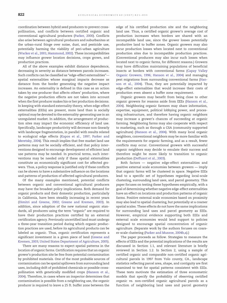
822 E C O L O G I C A L E C O N O M I C S 6 0 ( 2 0 0 7 ) 8 2 1 – 8 3 3

coordination between hybrid seed producers to prevent cross-pollination, and conflicts between certified organic andconventional agricultural producers (Parker, 2000). Conflictsalso arise between agricultural producers and suburbanites atthe urban–rural fringe over noise, dust, and pesticide use,potentially harming the viability of peri-urban agriculture(Wacker et al., 2001; Hammond, 2002). These incompatibilitiesmay influence grower location decisions, crops grown, andproduction practices.

All of the above examples exhibit distance dependence,decreasing in severity as distance between parcels increases.Such conflicts can be classified as “edge-effect externalities”—spatial externalities whose marginal impacts decrease asdistance from the border generating the negative impactincreases. An externality is defined in this case as an actiontaken by one producer that affects others' production, wherethe negative production effects are not taken into accountwhen the first producermakes his or her production decisions.In keeping with standard externality theory, when edge-effectexternalities (EEEs) are present, more land than is sociallyoptimalmaybe devoted to the externality-generating use in anunregulated market. In addition, the arrangement of produc-tion sites may impact the economic efficiency of land use.Specifically, landscape productivity will decrease non-linearlywith landscape fragmentation, in parallel with results relatedto ecological edge effects (Kapos et al., 1997; Parker andMeretsky, 2004). This result implies that free market land usepatterns may not be socially efficient, and that policy inter-ventions designed to encourage development of efficient landuse patterns may be needed. In practical terms, such inter-ventions may be needed only if these spatial externalitiesconstitute an economically significant cost for affected gro-wers. Thus, a policy response is justified only if these conflictscan be shown to have a substantive influence on the locationsand patterns of production of affected agricultural producers.

Of the many examples mentioned, potential conflictsbetween organic and conventional agricultural producersmay have the broadest policy implications. Both demand fororganic products and their domestic production, particularlyin California, have been steadily increasing in recent years(Dimitri and Greene, 2002; Greene and Kremen, 2003). Inaddition, since adoption of the new national organic stan-dards, all producers using the term “organic” are required tohave their production practices certified by an externalcertification agency. Previously uncertified landmust undergoa three-year transition period during which organic produc-tion practices are used, before its agricultural products can belabeled as organic. Thus, organic certification represents asignificant investment in a given piece of land (Greene andKremen, 2003; United States Department of Agriculture, 2005).

There are many reasons to expect spatial patterns in thelocationof organic farms. Certification requires that anorganicgrower's production site be free from potential contaminationby prohibited materials. One of the most probable sources ofcontamination can be spatial spillovers fromsurrounding landuses, including drift of prohibited chemicals or possible cross-pollination with genetically modified crops (Hanson et al.,2004). Therefore, in cases where an inspector determines thatcontamination is possible from a neighboring use, the organicproducer is required to leave a 25 ft. buffer zone between the

edge of his certified production site and the neighboringland use. Thus, a certified organic grower's average cost ofproduction increases when borders are shared with anincompatible land use, since the grower losses potentiallyproductive land to buffer zones. Organic growers may alsoincur production losses when located next to conventionalproduction sites due to incompatible production practices.(Conventional producers may also incur such losses whenlocated next to organic farms, for different reasons.) Growersmay have difficulties maintaining populations of beneficialinsects at borders with conventional farms (Capay ValleyOrganic Growers, 1996; Hanson et al., 2004) and managingpest migrations from surrounding conventional farms (Han-son et al., 2004). Thus, they are potentially impacted byedge-effect externalities that would increase their costs ofproduction even absent a buffer zone requirement.

Organic growers may benefit from being close to otherorganic growers for reasons aside from EEEs (Hanson et al.,2004). Neighboring organic farmers may share information,expertise, equipment, political lobbying power, and proces-sing infrastructure, and therefore having organic neighborsmay increase a grower's chances of succeeding at organicfarming. Neighboring farms may also cooperate with respectto marketing, such as through a CSA (community supportedagriculture) (Hanson et al., 2004). With many local organicneighbors, conventional neighbors may be more familiar withthe requirements for organic farming, and as a result, fewerconflicts may occur. Conventional growers with successfulorganic neighbors may decide to emulate their success andtherefore might be more likely to transition to organicproduction (Deffuant et al., 2003).

Both factors — negative edge-effect externalities andpositive external scale economies between growers — implythat organic farms will be clustered in space. Negative EEEslead to a specific set of hypotheses regarding local-scaleclustering, surrounding land uses, and parcel geometry. Thispaper focuses on testing these hypotheses empirically, with agoal of determiningwhether negative edge-effect externalitieshave an effect on locations and production patterns of organicfarms. Positive external scale economies based on proximitymay also lead to spatial clustering, but potentially at a coarserspatial scales. These effects do not have the same implicationsfor surrounding land uses and parcel geometry as EEEs.However, empirical evidence supporting both EEEs andexternal scale economies would lend support to policiesdesigned to encourage spatial concentration of organicagriculture. (Separate work by the authors focuses on coars-er-scale clustering (Parker and Munroe, 2004b,a).)

The paper proceeds as follow. Strategies to measure theeffects of EEEs and the potential implications of the results arediscussed in Section 1.1, and relevant literature is brieflyreviewed in Section 1.2. In Section 2, using a sample ofcertified organic and comparable non-certified organic agri-cultural parcels in 1997 from Yolo county, CA., landscapestatistics reflecting parcel area, shape, and contiguity are firstexamined to test for spatial patterns consistent with EEEs.These tests motivate the estimation of three econometricmodels that specify the probability of observing certifiedorganic vs. non-certified organic agricultural parcels as afunction of neighboring land uses and parcel geometry

823E C O L O G I C A L E C O N O M I C S 6 0 ( 2 0 0 7 ) 8 2 1 – 8 3 3

(Section 3). We find significant evidence to support thehypothesis of avoidance of EEEs. We conclude with analysisof the overall results, suggestions for further research, and adiscussion of policy implications.

1.1. Edge-effect externalities and land-use patterns

1.1.1. Measuring edge effect externalitiesThe concept of landscape fragmentation can be broad anddifficult to define. In the case of edge effects, however, theconcept has a concrete definition. Specifically, when alandscape pattern for a given area exhibits the fewest bordersshared between incompatible uses it will be most productive,and this landscape productivity will decrease non-linearly asthe proportion of incompatible borders in a landscapeincreases. The length of an incompatible border per unitarea, then, is a broad empirical measure of the impact of edgeeffects. This summary measure has been recognized for sometime by ecologists. However, within a landscape edge per unitarea varies according to several geographic dimensions, somerelated to the geometry of individual parcels and othersrelated to landscape relationships between parcels. At anindividual parcel level, these dimensions include parcel sizeand shape. At a landscape level, they include parcel contiguityand the distribution of land area between parcels (Parker andMeretsky, 2004).

The relatively abstract measure of incompatible borderlength per unit area translates into concrete terms in thecase of certified organic growers, since the costs of spatialspillovers can be proxied through land area in required bufferzones. While it would be ideal to calculate actual buffer costsdirectly, as that would allow tests related to the magnitude ofbuffer zone costs, data on yields and output prices fororganic products are not available due to confidentialityconstraints. As well, buffer zone costs may include transac-tion costs related to communication with neighbors (Parker,2000). For certified organic growers, costs due to buffer zoneswill increase as the proportion of their production land inmandatory buffer zones increases. Therefore, land in bufferzones as a percentage of total land area is a summarymeasure of the impact of edge-effect externalities on organicproduction sites, reflecting differences in both parcel geom-etry and surrounding land uses. It is sufficient to test thehypothesis that organic parcels differ from non-organicparcels in a manner consistent with avoidance of edge-effectexternalities.

Decomposing the possible geometric dimensions of frag-mentation in the case of organic farms may reveal additionalpolicy-relevant information. Do organic farmers avoid bufferzone losses by farming larger parcels than non-organic farms,implying that the optimal size for an organic farm may belarger than for a non-organic farm? Are organic parcelsinherently more compact than non-organic parcels? Anaffirmative answer to each of these questions would indicatethat the organic parcels have a lower border per unit area ratiothan conventional parcels.

A parcel with a high border per unit area ratio may notlose any production land to buffer zones if surrounding landuses do not pose a threat to the integrity of organicproduction. Therefore, a parcel bordering natural areas,

another organic farm, or roadways which provide sufficientbuffers from neighboring uses may be particularly attractiveto organic growers. This possibility raises additional policy-relevant questions related to organic parcels. Is an organicparcel more likely to border a potentially compatible landuse? If so, how much do surrounding land uses contributeto lower potential costs from buffer zones on organicparcels?

1.1.2. The geography of market failureInherent in this analysis of organic landscapes is thequestion of whether parcel geography reflects both individ-ual and cooperative cost-minimization with respect to bufferzones. On an individual basis, an organic grower has theability to minimize buffer costs through geographicallyconcentrating farm production, farming parcels with a lowratio of border per unit area, locating next to other non-organic but compatible land uses, and obtaining the cooper-ation of neighboring conventional farms in avoiding drift.The potential for returns to cooperation between organicgrowers exists as well. When organic growers farm parcelsnext to those farmed by other organic growers, each growergains the benefits of a border where no buffer zone isrequired. Thus, there are potential positive externalitiesbetween growers that can only be captured though sharedborders between separately managed organic farms. Inaddition, as discussed above, benefits from shared informa-tion, experience, and resources may lead to external scaleeconomies between growers.

The question addressed by this paper is not simplywhether spatial spillovers from conventional to organicfarms exist. Due to the imposition and enforcement ofmandatory buffer zones, these costs are concrete anddocumented. Rather, our ongoing work attempts to answertwo interlinked questions related to geographic aspects ofmarket failure. The first question is whether costs related tobuffer zones are sufficiently high to influence location andproduction decisions of individual organic growers. Thesecond question is whether the potential positive externalitiesbetween organic growers, both those induced by the existenceof negative spillovers from conventional to organic growersand those due to external scale economies, have led to thedevelopment of economically efficient clustering of separateorganic farms. The answer to these question may suggestwhether external policy interventions related to whole-landscape planning for zones of both organic and conven-tional production could be helpful.

1.2. Related literature

While development of spatially explicit empirical economicmodels is recent, methodological development has been fairlyrapid, with land-use modeling leading the way. There is anincreasing recognition that land-use decisions occur in adynamic spatial landscape, where land users interact witheach other within a heterogeneous spatial environment. Twoexcellent reviews of recent research in this area are providedby Nelson and Geoghegan (2002) and Bell and Irwin (2002). Forthe most part, the goal of recent empirical studies that utilizespatially explicit economic and physical information has been


to predict land use or land-use transitions at a fine spatialscale. Their general approach has been to generate indepen-dent variables reflecting spatial relationships using a GIS.These variables enter into a limited dependent variable modelto test how each factor contributes to the probability of findingland in a particular use. The degree of disaggregation of landuses and use of spatial information varies with the studies.Most closely related to this paper are two research projectsthat specifically test for negative effects of surrounding landuses on property values. Palmquist et al. (1997) use a hedonicmodel to estimate the price gradient of residential propertyvalues as a function of distance from hog operations, a sourceof substantial negative externalities. They find statisticallysignificant increases in property values as distance to the hogoperations increases. Bockstael and her colleagues (Bockstael,1996; Geoghegan et al., 1996, 1997; Irwin and Bockstael, 2002)have published several papers that test for influences ofsurrounding land uses on property values and the probabilityof conversion of undeveloped land. Consistent with expecta-tions, they have found that land values and conversionprobabilities increase with the proportion of surroundingopen space and pasture and decrease with the proportion incropland and the length of incompatible edges. Leggett andBockstael (2000) link localized variations in water quality totheir negative impacts on residential property values. Furtherwork has considered the impacts of landscape pattern onproperty values using some landscape ecology statistics suchas fractal dimension (Geoghegan et al., 1997). However, theseauthors have not developed explicit theoretical predictionsthat link landscape pattern and property values.

This paper contributes to the growing literature onempirical economic spatial analysis in two important aspects.First, this particular empirical application offers promise forisolating and measuring impacts of negative externalities. Inurban and residential settings, any one property is most likelyinfluenced by many different surrounding land uses. In theagricultural setting examined in this paper, given that parcelsizes are large relative to the dispersal radius of potentialnegative externalities, few surrounding uses potentiallyimpact a particular parcel. Second, estimation of propertyvalue impacts requires the use of hedonic techniques. In orderfor hedonic estimates to correctly reflect the impact ofsurrounding land uses, all other relevant influences must becontrolled for. In this study, externality impacts can bemeasured directly through examination of buffer zonerequirements. Further, this paper is the first to includevariables reflecting landscape pattern that are explicitlyderived from a theoretical economic framework.

2. Data

2.1. Data sources and sampling methods

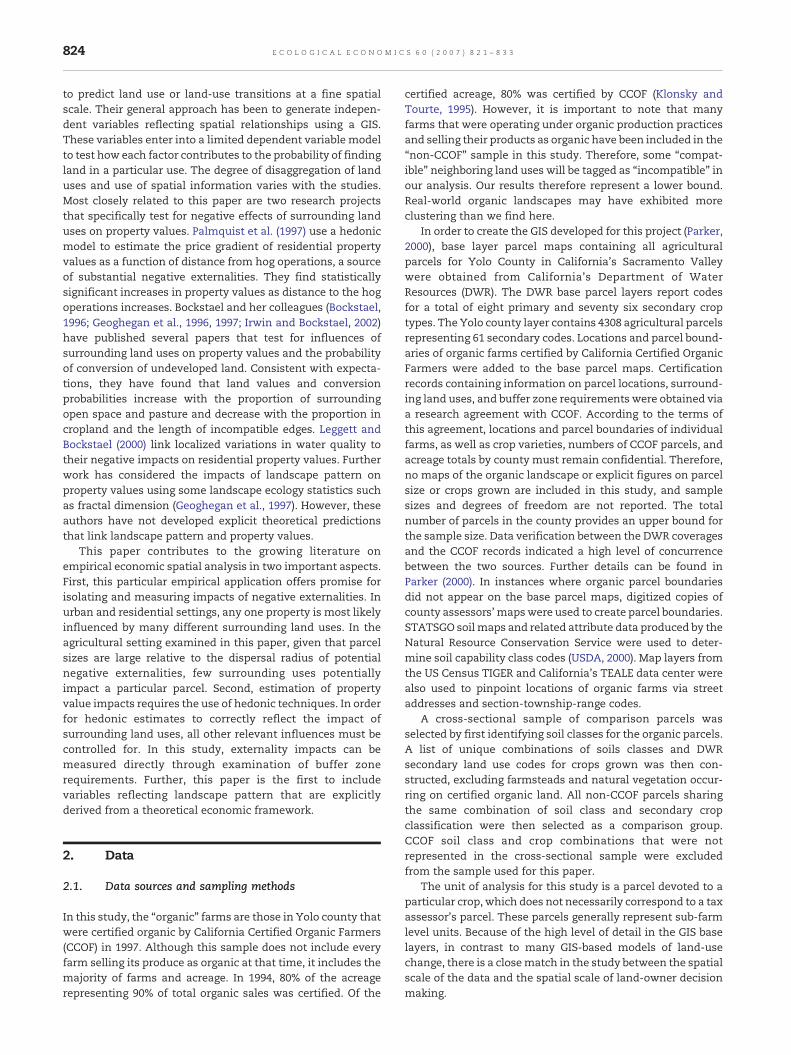
In this study, the “organic” farms are those in Yolo county thatwere certified organic by California Certified Organic Farmers(CCOF) in 1997. Although this sample does not include everyfarm selling its produce as organic at that time, it includes themajority of farms and acreage. In 1994, 80% of the acreagerepresenting 90% of total organic sales was certified. Of the

certified acreage, 80% was certified by CCOF (Klonsky andTourte, 1995). However, it is important to note that manyfarms that were operating under organic production practicesand selling their products as organic have been included in the“non-CCOF” sample in this study. Therefore, some “compat-ible” neighboring land uses will be tagged as “incompatible” inour analysis. Our results therefore represent a lower bound.Real-world organic landscapes may have exhibited moreclustering than we find here.

In order to create the GIS developed for this project (Parker,2000), base layer parcel maps containing all agriculturalparcels for Yolo County in California's Sacramento Valleywere obtained from California's Department of WaterResources (DWR). The DWR base parcel layers report codesfor a total of eight primary and seventy six secondary croptypes. The Yolo county layer contains 4308 agricultural parcelsrepresenting 61 secondary codes. Locations and parcel bound-aries of organic farms certified by California Certified OrganicFarmers were added to the base parcel maps. Certificationrecords containing information on parcel locations, surround-ing land uses, and buffer zone requirements were obtained viaa research agreement with CCOF. According to the terms ofthis agreement, locations and parcel boundaries of individualfarms, as well as crop varieties, numbers of CCOF parcels, andacreage totals by county must remain confidential. Therefore,no maps of the organic landscape or explicit figures on parcelsize or crops grown are included in this study, and samplesizes and degrees of freedom are not reported. The totalnumber of parcels in the county provides an upper bound forthe sample size. Data verification between the DWR coveragesand the CCOF records indicated a high level of concurrencebetween the two sources. Further details can be found inParker (2000). In instances where organic parcel boundariesdid not appear on the base parcel maps, digitized copies ofcounty assessors' mapswere used to create parcel boundaries.STATSGO soil maps and related attribute data produced by theNatural Resource Conservation Service were used to deter-mine soil capability class codes (USDA, 2000). Map layers fromthe US Census TIGER and California's TEALE data center werealso used to pinpoint locations of organic farms via streetaddresses and section-township-range codes.

A cross-sectional sample of comparison parcels wasselected by first identifying soil classes for the organic parcels.A list of unique combinations of soils classes and DWRsecondary land use codes for crops grown was then con-structed, excluding farmsteads and natural vegetation occur-ring on certified organic land. All non-CCOF parcels sharingthe same combination of soil class and secondary cropclassification were then selected as a comparison group.CCOF soil class and crop combinations that were notrepresented in the cross-sectional sample were excludedfrom the sample used for this paper.

The unit of analysis for this study is a parcel devoted to aparticular crop, which does not necessarily correspond to a taxassessor's parcel. These parcels generally represent sub-farmlevel units. Because of the high level of detail in the GIS baselayers, in contrast to many GIS-based models of land-usechange, there is a closematch in the study between the spatialscale of the data and the spatial scale of land-owner decisionmaking.

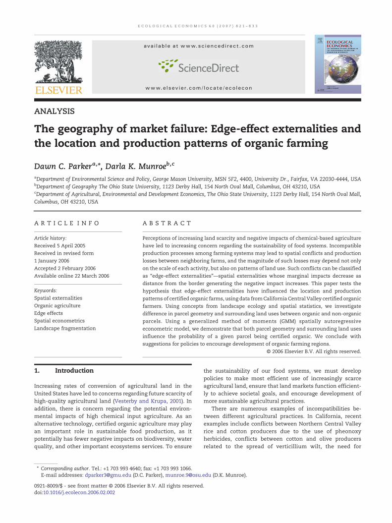
Neighbor Maintains Buffer

+ Organic Grower's Land=Certified Organic Production Area

Land in Mandatory Buffer

Incompatible Land Use Natural Vegetation

Fig. 1 –Key for Figs. 2–5.


2.2. Spatial descriptive statistics

A series of statistics reflecting parcel geometry and neighbor-ing land uses are presented below. Potential productionimpacts are illustrated by linking variations in parcel geogra-phy to percentage of area lost to buffer zones. This analysisprovides preliminary evidence related to the effect of EEEs,and motivates specification of the econometric model.

2.2.1. Parcel geometryThe following examples illustrate the impacts of parcelcontiguity, parcel size, and parcel shape on production underthe assumption that buffers are required on all exposedborders. Area concentration is an additional relevant geo-graphic dimension, as discussed by Parker and Meretsky(2004). Concentration results are reported by Parker (2000).This illustration outlines possible losses to buffer zonesindependent of the effects of surrounding land uses. In effect,it illustrates potential losses that would occur if each parcelwere surrounded by incompatible uses.

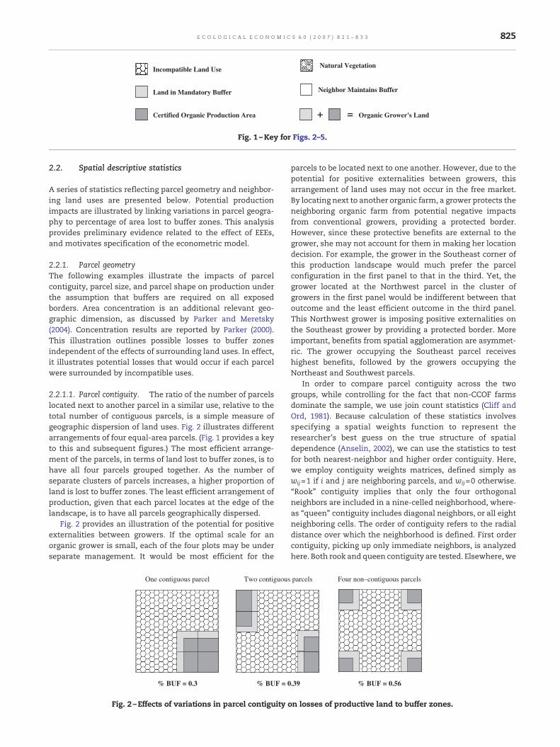
2.2.1.1. Parcel contiguity. The ratio of the number of parcelslocated next to another parcel in a similar use, relative to thetotal number of contiguous parcels, is a simple measure ofgeographic dispersion of land uses. Fig. 2 illustrates differentarrangements of four equal-area parcels. (Fig. 1 provides a keyto this and subsequent figures.) The most efficient arrange-ment of the parcels, in terms of land lost to buffer zones, is tohave all four parcels grouped together. As the number ofseparate clusters of parcels increases, a higher proportion ofland is lost to buffer zones. The least efficient arrangement ofproduction, given that each parcel locates at the edge of thelandscape, is to have all parcels geographically dispersed.

Fig. 2 provides an illustration of the potential for positiveexternalities between growers. If the optimal scale for anorganic grower is small, each of the four plots may be underseparate management. It would be most efficient for the

% BUF = 0% BUF = 0.3

Two contiguousOne contiguous parcel

Fig. 2 –Effects of variations in parcel contiguity o

parcels to be located next to one another. However, due to thepotential for positive externalities between growers, thisarrangement of land uses may not occur in the free market.By locating next to another organic farm, a grower protects theneighboring organic farm from potential negative impactsfrom conventional growers, providing a protected border.However, since these protective benefits are external to thegrower, she may not account for them in making her locationdecision. For example, the grower in the Southeast corner ofthis production landscape would much prefer the parcelconfiguration in the first panel to that in the third. Yet, thegrower located at the Northwest parcel in the cluster ofgrowers in the first panel would be indifferent between thatoutcome and the least efficient outcome in the third panel.This Northwest grower is imposing positive externalities onthe Southeast grower by providing a protected border. Moreimportant, benefits from spatial agglomeration are asymmet-ric. The grower occupying the Southeast parcel receiveshighest benefits, followed by the growers occupying theNortheast and Southwest parcels.

In order to compare parcel contiguity across the twogroups, while controlling for the fact that non-CCOF farmsdominate the sample, we use join count statistics (Cliff andOrd, 1981). Because calculation of these statistics involvesspecifying a spatial weights function to represent theresearcher's best guess on the true structure of spatialdependence (Anselin, 2002), we can use the statistics to testfor both nearest-neighbor and higher order contiguity. Here,we employ contiguity weights matrices, defined simply aswij=1 if i and j are neighboring parcels, and wij=0 otherwise.“Rook” contiguity implies that only the four orthogonalneighbors are included in a nine-celled neighborhood, where-as “queen” contiguity includes diagonal neighbors, or all eightneighboring cells. The order of contiguity refers to the radialdistance over which the neighborhood is defined. First ordercontiguity, picking up only immediate neighbors, is analyzedhere. Both rook and queen contiguity are tested. Elsewhere, we

.39 % BUF = 0.56

parcels Four non–contiguous parcels

n losses of productive land to buffer zones.

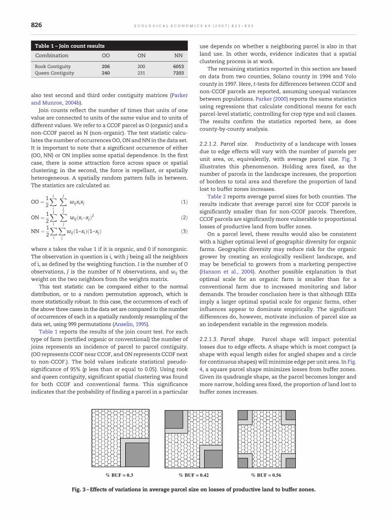
Table 1 – Join count results

Combination OO ON NN

Rook Contiguity 206 200 6053Queen Contiguity 240 231 7203


also test second and third order contiguity matrices (Parkerand Munroe, 2004b).

Join counts reflect the number of times that units of onevalue are connected to units of the same value and to units ofdifferent values. We refer to a CCOF parcel as O (organic) and anon-CCOF parcel as N (non-organic). The test statistic calcu-lates thenumber of occurrencesOO,ONandNN in the data set.It is important to note that a significant occurrence of either(OO, NN) or ON implies some spatial dependence. In the firstcase, there is some attraction force across space or spatialclustering; in the second, the force is repellant, or spatiallyheterogeneous. A spatially random pattern falls in between.The statistics are calculated as:

OO ¼ 12

XI

i

XJ

j

wijxixj ð1Þ

ON ¼ 12

XI

i

XJ

j

wijðxi−xjÞ2 ð2Þ

NN ¼ 12

X

i

X

j

wijð1−xiÞð1−xjÞ ð3Þ

where x takes the value 1 if it is organic, and 0 if nonorganic.The observation in question is i, with j being all the neighborsof i, as defined by the weighting function. I is the number of Oobservations, J is the number of N observations, and wij theweight on the two neighbors from the weights matrix.

This test statistic can be compared either to the normaldistribution, or to a random permutation approach, which ismore statistically robust. In this case, the occurrences of each ofthe above three cases in the data set are compared to the numberof occurrences of each in a spatially randomly resampling of thedata set, using 999 permutations (Anselin, 1995).

Table 1 reports the results of the join count test. For eachtype of farm (certified organic or conventional) the number ofjoins represents an incidence of parcel to parcel contiguity.(OO represents CCOF near CCOF, and ON represents CCOF nextto non-CCOF.). The bold values indicate statistical pseudo-significance of 95% (p less than or equal to 0.05). Using rookand queen contiguity, significant spatial clustering was foundfor both CCOF and conventional farms. This significanceindicates that the probability of finding a parcel in a particular

% BUF = 0.3 % BUF =

Fig. 3 –Effects of variations in average parcel size

use depends on whether a neighboring parcel is also in thatland use. In other words, evidence indicates that a spatialclustering process is at work.

The remaining statistics reported in this section are basedon data from two counties, Solano county in 1994 and Yolocounty in 1997. Here, t-tests for differences between CCOF andnon-CCOF parcels are reported, assuming unequal variancesbetween populations. Parker (2000) reports the same statisticsusing regressions that calculate conditional means for eachparcel-level statistic, controlling for crop type and soil classes.The results confirm the statistics reported here, as doescounty-by-county analysis.

2.2.1.2. Parcel size. Productivity of a landscape with lossesdue to edge effects will vary with the number of parcels perunit area, or, equivalently, with average parcel size. Fig. 3illustrates this phenomenon. Holding area fixed, as thenumber of parcels in the landscape increases, the proportionof borders to total area and therefore the proportion of landlost to buffer zones increases.

Table 2 reports average parcel sizes for both counties. Theresults indicate that average parcel size for CCOF parcels issignificantly smaller than for non-CCOF parcels. Therefore,CCOF parcels are significantlymore vulnerable to proportionallosses of productive land from buffer zones.

On a parcel level, these results would also be consistentwith a higher optimal level of geographic diversity for organicfarms. Geographic diversity may reduce risk for the organicgrower by creating an ecologically resilient landscape, andmay be beneficial to growers from a marketing perspective(Hanson et al., 2004). Another possible explanation is thatoptimal scale for an organic farm is smaller than for aconventional farm due to increased monitoring and labordemands. The broader conclusion here is that although EEEsimply a larger optimal spatial scale for organic farms, otherinfluences appear to dominate empirically. The significantdifferences do, however, motivate inclusion of parcel size asan independent variable in the regression models.

2.2.1.3. Parcel shape. Parcel shape will impact potentiallosses due to edge effects. A shape which is most compact (ashape with equal length sides for angled shapes and a circlefor continuous shapes)willminimize edge per unit area. In Fig.4, a square parcel shape minimizes losses from buffer zones.Given its quadrangle shape, as the parcel becomes longer andmore narrow, holding area fixed, the proportion of land lost tobuffer zones increases.

% BUF = 0.56 0.42

on losses of productive land to buffer zones.

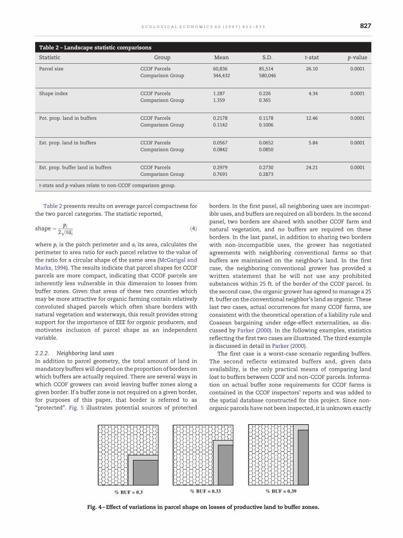
Table 2 – Landscape statistic comparisons

Statistic Group Mean S.D. t-stat p-value

Parcel size CCOF Parcels 60,836 85,514 26.10 0.0001Comparison Group 344,432 580,046

Shape index CCOF Parcels 1.287 0.226 4.34 0.0001Comparison Group 1.359 0.365

Pot. prop. land in buffers CCOF Parcels 0.2178 0.1178 12.46 0.0001Comparison Group 0.1142 0.1006

Est. prop. land in buffers CCOF Parcels 0.0567 0.0652 5.84 0.0001Comparison Group 0.0842 0.0850

Est. prop. buffer land in buffers CCOF Parcels 0.2979 0.2730 24.21 0.0001Comparison Group 0.7691 0.2873

t-stats and p-values relate to non-CCOF comparison group.


Table 2 presents results on average parcel compactness forthe two parcel categories. The statistic reported,

shape ¼ pi2

ffiffiffiffiffiffiffipai

p ð4Þ

where pi is the patch perimeter and ai its area, calculates theperimeter to area ratio for each parcel relative to the value ofthe ratio for a circular shape of the same area (McGarigal andMarks, 1994). The results indicate that parcel shapes for CCOFparcels are more compact, indicating that CCOF parcels areinherently less vulnerable in this dimension to losses frombuffer zones. Given that areas of these two counties whichmay be more attractive for organic farming contain relativelyconvoluted shaped parcels which often share borders withnatural vegetation and waterways, this result provides strongsupport for the importance of EEE for organic producers, andmotivates inclusion of parcel shape as an independentvariable.

2.2.2. Neighboring land usesIn addition to parcel geometry, the total amount of land inmandatory bufferswill depend on the proportion of borders onwhich buffers are actually required. There are several ways inwhich CCOF growers can avoid leaving buffer zones along agiven border. If a buffer zone is not required on a given border,for purposes of this paper, that border is referred to as“protected”. Fig. 5 illustrates potential sources of protected

% BUF = 0.3 % BUF

Fig. 4 –Effect of variations in parcel shape on

borders. In the first panel, all neighboring uses are incompat-ible uses, and buffers are required on all borders. In the secondpanel, two borders are shared with another CCOF farm andnatural vegetation, and no buffers are required on theseborders. In the last panel, in addition to sharing two borderswith non-incompatible uses, the grower has negotiatedagreements with neighboring conventional farms so thatbuffers are maintained on the neighbor's land. In the firstcase, the neighboring conventional grower has provided awritten statement that he will not use any prohibitedsubstances within 25 ft. of the border of the CCOF parcel. Inthe second case, the organic grower has agreed tomanage a 25ft. buffer on the conventional neighbor's land as organic. Theselast two cases, actual occurrences for many CCOF farms, areconsistent with the theoretical operation of a liability rule andCoasean bargaining under edge-effect externalities, as dis-cussed by Parker (2000). In the following examples, statisticsreflecting the first two cases are illustrated. The third exampleis discussed in detail in Parker (2000).

The first case is a worst-case scenario regarding buffers.The second reflects estimated buffers and, given dataavailability, is the only practical means of comparing landlost to buffers between CCOF and non-CCOF parcels. Informa-tion on actual buffer zone requirements for CCOF farms iscontained in the CCOF inspectors' reports and was added tothe spatial database constructed for this project. Since non-organic parcels have not been inspected, it is unknown exactly

% BUF = 0.39= 0.33

losses of productive land to buffer zones.

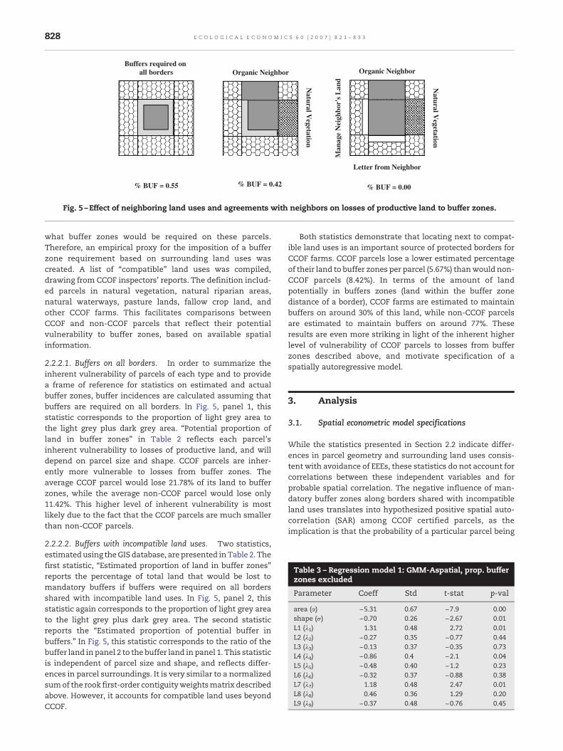
Table 3 – Regression model 1: GMM-Aspatial, prop. bufferzones excluded

Parameter Coeff Std t-stat p-val

area (α) −5.31 0.67 −7.9 0.00shape (σ) −0.70 0.26 −2.67 0.01L1 (λ1) 1.31 0.48 2.72 0.01L2 (λ2) −0.27 0.35 −0.77 0.44L3 (λ3) −0.13 0.37 −0.35 0.73L4 (λ4) −0.86 0.4 −2.1 0.04L5 (λ5) −0.48 0.40 −1.2 0.23L6 (λ6) −0.32 0.37 −0.88 0.38L7 (λ7) 1.18 0.48 2.47 0.01L8 (λ8) 0.46 0.36 1.29 0.20L9 (λ9) −0.37 0.48 −0.76 0.45

Natural V

egetation

Man

age

Nei

ghbo

r's

Lan

d

Letter from Neighbor

Organic NeighborOrganic Neighbor

Natural V

egetation

Buffers required on all borders

% BUF = 0.42 % BUF = 0.00% BUF = 0.55

Fig. 5 –Effect of neighboring land uses and agreements with neighbors on losses of productive land to buffer zones.


what buffer zones would be required on these parcels.Therefore, an empirical proxy for the imposition of a bufferzone requirement based on surrounding land uses wascreated. A list of “compatible” land uses was compiled,drawing from CCOF inspectors' reports. The definition includ-ed parcels in natural vegetation, natural riparian areas,natural waterways, pasture lands, fallow crop land, andother CCOF farms. This facilitates comparisons betweenCCOF and non-CCOF parcels that reflect their potentialvulnerability to buffer zones, based on available spatialinformation.

2.2.2.1. Buffers on all borders. In order to summarize theinherent vulnerability of parcels of each type and to providea frame of reference for statistics on estimated and actualbuffer zones, buffer incidences are calculated assuming thatbuffers are required on all borders. In Fig. 5, panel 1, thisstatistic corresponds to the proportion of light grey area tothe light grey plus dark grey area. “Potential proportion ofland in buffer zones” in Table 2 reflects each parcel'sinherent vulnerability to losses of productive land, and willdepend on parcel size and shape. CCOF parcels are inher-ently more vulnerable to losses from buffer zones. Theaverage CCOF parcel would lose 21.78% of its land to bufferzones, while the average non-CCOF parcel would lose only11.42%. This higher level of inherent vulnerability is mostlikely due to the fact that the CCOF parcels are much smallerthan non-CCOF parcels.

2.2.2.2. Buffers with incompatible land uses. Two statistics,estimatedusing theGIS database, are presented inTable 2. Thefirst statistic, “Estimated proportion of land in buffer zones”reports the percentage of total land that would be lost tomandatory buffers if buffers were required on all bordersshared with incompatible land uses. In Fig. 5, panel 2, thisstatistic again corresponds to the proportion of light grey areato the light grey plus dark grey area. The second statisticreports the “Estimated proportion of potential buffer inbuffers.” In Fig. 5, this statistic corresponds to the ratio of thebuffer land in panel 2 to the buffer land in panel 1. This statisticis independent of parcel size and shape, and reflects differ-ences in parcel surroundings. It is very similar to a normalizedsumof the rook first-order contiguityweightsmatrix describedabove. However, it accounts for compatible land uses beyondCCOF.

Both statistics demonstrate that locating next to compat-ible land uses is an important source of protected borders forCCOF farms. CCOF parcels lose a lower estimated percentageof their land to buffer zones per parcel (5.67%) thanwould non-CCOF parcels (8.42%). In terms of the amount of landpotentially in buffers zones (land within the buffer zonedistance of a border), CCOF farms are estimated to maintainbuffers on around 30% of this land, while non-CCOF parcelsare estimated to maintain buffers on around 77%. Theseresults are even more striking in light of the inherent higherlevel of vulnerability of CCOF parcels to losses from bufferzones described above, and motivate specification of aspatially autoregressive model.

3. Analysis

3.1. Spatial econometric model specifications

While the statistics presented in Section 2.2 indicate differ-ences in parcel geometry and surrounding land uses consis-tent with avoidance of EEEs, these statistics do not account forcorrelations between these independent variables and forprobable spatial correlation. The negative influence of man-datory buffer zones along borders shared with incompatibleland uses translates into hypothesized positive spatial auto-correlation (SAR) among CCOF certified parcels, as theimplication is that the probability of a particular parcel being

Table 4 – Regression model 2: GMM-Aspatial, prop. bufferzones included

Parameter Coeff Std t-stat p-val

area (α) −4.12 0.56 −7.17 0.00shape (σ) −0.85 0.32 −2.66 0.01badbpot (β) −2.17 0.16 −13.68 0.00L1 (λ1) 2.46 0.56 4.39 0.00L2 (λ2) 0.96 0.43 2.23 0.03L3 (λ3) 1.35 0.46 2.95 0.00L4 (λ4) 0.45 0.51 0.89 0.37L5 (λ5) 0.30 0.48 0.63 0.53L6 (λ6) 0.54 0.46 1.19 0.23L7 (λ7) 2.35 0.57 4.13 0.00L8 (λ8) 1.88 0.44 4.31 0.00L9 (λ9) 1.20 0.56 2.14 0.03

Table 5 – Regression model 3: GMM-SAR, prop. bufferzones excluded

Parameter Coeff Std Err t-stat p-val

area (α) −4.04 1.24 −3.26 0.00shape (σ) −0.45 0.56 −0.8 0.42L1 (λ1) −1.39 1.059 −1.31 0.19L2 (λ2) −2.13 0.78 −2.74 0.01L3 (λ3) −1.63 0.77 −2.12 0.03


CCOF increases if the neighboring parcel is also CCOF. Thisproblem is potentially serious from a statistical standpoint, asinclusion of a spatial lag variable without explicit correctionfor spatial dependence within the covariance matrix impliesbiased coefficient estimates (Anselin, 1988). As well, we arespecifically interested in the magnitude and significance ofthe spatial autocorrelation coefficient.

While techniques for estimating spatial correlation incontinuous dependent variable models are now fairly welldeveloped, and code for estimation is widely available,development of techniques and code for limited dependentvariable spatial models has lagged behind (Fleming, 2002,2004). However, substantial recent progress has been made,reviewed by Fleming (2004).

We present three econometric models, which representprogressive improvements in the extent to which theyaccount for spatial relationships. Model results presented inTables 3–5 include: 1) an aspatial Generalized Method ofMoments (GMM) model that excludes the effects of surround-ing land uses; 2) an aspatial GMM that includes the estimatedproportion of potential buffer land in buffer zones (“badbpot”);and 3) a spatially autoregressive GMM, with “badbpot”excluded but a first-order spatial lag included. The equationsfor the three models are:

Model 1 : PrðYi;j ¼ 1Þ ¼ Fða areaþ r shapeþ Lkþ eÞ ð5ÞModel 2 : PrðYi;j ¼ 1Þ ¼ Fða areaþ r shapeþ Lk

þ b badbpotþ eÞ ð6ÞModel 3 : PrðYi;j ¼ 1Þ ¼ Fða areaþ r shapeþ Lkþ YN

i;jqþ eÞ ð7Þ

where F is the cumulative probability density function, Yi,j

equals to 1 if a parcel at spatial location i, j is CCOF, 0 otherwiseand Yi;j

Nρ is the first-order contiguity matrix times theestimated spatial autocorrelation coefficient.

The independent variables1 are:

area: parcel area from Section 2.2.1.2shape: parcel shape index from Section 2.2.1.3L1: citrus and subtropical

1 While we have information on soil capability class, modelsthat included this variable would not converge, likely due to littlevariation in soils, so that variable was omitted. (97% of the entiresample was from the same soil type.)

L2: deciduous fruits and nutsL3: field cropsL4: grain and hay cropsL5: idleL6: pastureL7: riceL8: truck, nursery and berry cropsL9: vineyardsbadbpot: the proportion of potential buffer land estimated to

be in mandatory buffers from Section 2.2.2.2.

3.2. Results

In both Model 1 and Model 2, the variables related to parcelgeometry have the expected signs and are significant,indicating that CCOF parcels are smaller and more compactthan non-CCOF parcels. In Model 2, the coefficient onbadbpot is negative and highly significant, as expected,indicating that the higher the proportion of borders a parcelshares with a potentially incompatible land use, the lesslikely that parcel is to be a CCOF parcel. However, thiscoefficient estimate is likely influenced by unmodeled spatialcorrelation. The Kelejian–Prucha Moran's I was computed forboth Model 1 and Model 2 (Kelejian and Prucha, 2001),resulting in values of 35.59 for Model 1 and 15.02 for Model 2.These tests indicate significant spatial correlation for bothmodels, with less spatial correlation in the model thatincludes “badbpot” reflecting the influence of surroundingland uses, as expected.

To account for spatial autocorrelation, in Model 3, we applya non-linear generalized least squares estimator derived usingGeneralized Methods of Moments techniques, as detailed inFleming (2004). TheGMMapproachallows for the estimationofthe spatially autoregressive parameter without having tocompute the Jacobian of the spatial covariance matrix, whichis computationally intensive for nonlinear probability models.This SARmodel provides consistent and efficient estimates ofthe non-spatial variables, and a consistent but inefficientestimate of the spatial lag parameter. The model is estimatedusing a first-order rook contiguity weights matrix, measuringthe nearest-neighbor effects of shared borders between CCOFand non-CCOF parcels potentially related to buffer zones.Because the “badbpot” variable is highly collinear with the

L4 (λ4) −2.21 0.88 −2.51 0.01L5 (λ5) −2.14 1.013 −2.11 0.03L6 (λ6) −1.98 0.89 −2.23 0.03L7 (λ7) −0.77 0.91 −0.84 0.40L8 (λ8) −1.20 0.73 −1.64 0.10L9 (λ9) −1.85 1.37 −1.35 0.18ρ 5.44 0.54 10.17 0

Table 6 – In-sample goodness of fit

Model 1: GMM-Aspatial, Prop. buffer zones excluded

PredictedConv. Organic Total

Actual Conv. 0.952 0.002 0.954Organic 0.044 0.002 0.046Total 0.996 0.004 1

Predicted/Actual 1.044 0.090 0.954

Kappa statistic 0.082

Model 2: GMM-Aspatial, Prop. buffer zones included





Model 3: GMM-SAR, Prop. buffer zones excluded





2 Pontius (2000) and Walker (2003) have pointed out limitationsof Kappa for assessing location prediction and predictive power.Many additional measures are available for spatial modelvalidation, focusing on prediction of location and pattern acrossspatial scales (Turner et al., 1989; Pontius, 2000). Because thecentral research question of this paper concerns parcel-to-parcelcontiguity, and not location prediction, we do not apply thosemeasures here. A possible extension to this paper could evaluatethe success of the model at replicating coarser-scale spatialpatterns of organic farms. That application would employ a widerrange of spatial goodness of fit measures.


spatial lag variable, this variable is excluded from the SARmodel.

The spatial lag parameter estimate, ρ, is positive andsignificant as expected. This variable may also be picking upunmodeled spatial error correlation, due to omitted variablesthat may also be spatially correlated, so its true magnitudeand significance level may be lower than estimated in thismodel. In combination with the results of Model 2, however,it strongly supports the hypothesis that the probability ofCCOF parcel declines when neighboring parcels are notcertified organic.

It is interesting to note that, compared to Model 1 andModel 2, when spatial correlation is accounted for, themagnitude and significance of the parcel geometry coeffi-cients, shape and area, are reduced. In fact, shape is nolonger significant. These results are consistent with thosefound by Case (1992), who demonstrates that failing toaccount for spatial error correlation results in overestimat-ing the influence of spatially correlated independentvariables.

Table 6 displays the cross-tabulation matrix, normalizedby the number of observation in the sample, generated forregressions. This matrix reports proportion of correct in-sample predictions for each category (conventional ororganic agriculture) for each model. Values on the diagonalare observations correctly predicted. There are two types oferror: omission (e.g., observations that were actually organicagriculture but predicted as conventional agriculture, in the

lower left cells) and commission errors (e.g., observationsthat were predicted as organic agriculture, but were actuallyconventional, in the upper right cells). The overall accuracyis the ratio of total correct predictions to the overall numberof observations (Predicted/Actual–Total). A last helpfulmeasure of accuracy is the Kappa statistic. The Kappastatistic ranges between 0 and 1 and measures theagreement between the model predictions and actual datarelative to the agreement that might be attained solely bychance matching, based on the proportional representationof each category in the data (Jensen, 1996). This statistic hasbeen previously used to evaluate spatial accuracy of landuse models (Nelson and Hellerstein, 1997; Walker, 2003).2

This table illustrates the importance of surrounding landuses for model fit. While all models are fairly successful atcorrectly predicting conventional parcels, Model 1 doesextremely poorly at predicting organic parcels, correctlypredicting only around 9%. In spite of uncorrected spatialcorrelation in the error structure, Model 2 is most successful atpredicting organic parcels, correctly predicting 68%. Since thismodel accounts for the influence of both protective land uses(organic and non-farm compatible uses), this fit is notsurprising. Although the model does not account for non-farm compatible uses, Model 3 is also fairly successful atpredicting organic, correctly predicting around 55%. Accordingto the total predicted/actual ratio and the Kappa statistic,Model 3 is the best fit, followed by Model 2 and Model 1.

3.3. Model limitations and next steps

While model results point to the importance of parcelgeometry and local surroundings for location of organicproduction sites, some limitations of the current modelsmust be acknowledged. The protective influences of naturalareas are not specifically estimated in Model 3. Developmentof a model that includes the natural areas, but is stillstatistically robust, is a priority for future work. Third, sincethese models use only first-order contiguity matrices, higher-order spatial clustering indicating potential positive externalscale economies cannot be assessed. Estimation of modelsusing the alternative spatial weights matrices discussed inSection 2.2.1.1 is an additional area for further work. Finally,ideally, a combined spatial error and spatial autocorrelationmodel would be estimated. While a reliable version of such amodel is not yet widely available, this approach is a logicalfuture step.

The models presented here essentially take the proportionof certified and non-certified organic agricultural productionin the region as given, since they do not include variables


reflecting the differential profitability of organic and conven-tional agriculture. Such variables would be based on thestandard von Thünen/Ricardo framework that land is devotedto its highest valued use, accounting for travel costs tomarket,and would include both estimated returns from organic andconventional production. Cost data needed to constructprofitability measures for organic agriculture for this timeperiod do not exist. Further, it seems unlikely that travel costswould be a significant determinant of location at such a smallscale.

Buffer zone requirements for organic growers were insti-tuted in 1990 after the passage of the California Organic Foodsact. Certification records indicated that between that time andthe time of this study (1997) some growers left organiccertification due to conflicts with neighboring land uses, andothers relocated to more protected locations. These changesoccurred over a period of years, as growers and certifiersbecame aware of potential conflicts and attempted to remedythem. Further, many growers may initially have requiredbuffers on many of their borders, but over time, they forgedagreements with neighbors so that buffer zones were notrequired (see Parker (2000) for further details). It is thereforelikely that the incidence of buffers in these landscapes ishigher and concentration of organic production lower thanwould be seen in a landscape where complete adjustment tobuffer requirements had occurred. In an ideal world, a space-time model would be constructed to examine this process oftransition. While a time series data set could be constructedfor the organic parcels if agricultural base layers wereavailable, unfortunately, a time series for the base layers isnot available.

An ideal empirical study would also examine whetherprotected locations captured high land rents by organicgrowers, as predicted by Parker (2004). Again, data on landvalues are not available for the region in GIS format.

4. Discussion and conclusions

All of the analysis presented here provides evidence thatfinding a location protected from potentially incompatibleuses is an important factor for certified organic farmers.Parcels farmed by certified growers, while inherently morevulnerable to proportional losses of productive land frombuffer zones than comparable non-certified organic parcels,appear relatively protected from losses due to buffer zones. Onfirst glance this appears to be an optimistic finding. A positiveinterpretation is that buffer zone regulations are not havingsubstantial impacts on the economic viability of organicproduction. A naive interpretation would be that externalityimpacts are mitigated through the efforts of organic growers,implying that welfare losses due to the spatial externalitiesare negligible.

However, this optimistic interpretation fails to considerthis case in the context of theoretical results related toexternalities in general and edge-effect externalities inparticular. Land-use pattern in the observed landscapesreflects market decisions based on private incentives. Intheory, market price distortions occur under externalities,with the result of too much production from the externality-

generation use occurring, and too little production occurringfrom the externality-receiving use (Baumol and Oates, 1988),relative to the socially optimal outcome. In the case of edge-effect externalities, this price distortion takes a particularform. As demonstrated by Parker (2004), in a free-marketoutcome without complete bargaining, the value of operat-ing free from the externality found in a protected locationwill be capitalized into the market rental rate of land. In thisparticular case, CCOF growers' bids for protected locationswill be increased by the value of the damage avoided. Theserelatively higher land rental rates for organic producers maypush less efficient organic growers out of the certifiedorganic market. The loss of these growers reflects thelower production by the organic industry theoreticallyexpected under externalities. As well, the avoidance behav-ior of potential externality damage demonstrated by CCOFfarmers does not imply that market distortions due toexternality damage are reduced. Externality avoidance doesnot equal externality mitigation (Freeman, 1994; Parker,2004).

However, this avoidance behavior by CCOF growers maycontribute to a relatively efficient landscape of organicfarming. Parker (1999) demonstrated that under edge-effectexternalities, while the free market may lead to globallyinefficient patterns of production, locally, parcel geometrywillbe relatively efficient. More specifically, production may bedispersed among several geographically isolated productionsites, but production patterns may evolve which minimizeincompatible borders with incompatible uses at individualsites. This theoretical prediction appears to hold in the case ofCCOF farmers. Farmers do not appear to have captured gainsfrom cooperation, since very few CCOF farms share borderswith other CCOF farms (Parker, 2000). Yet, individual farmersappear to be very successful at avoiding losses of productiveland from buffer zones.

The failure of CCOF farms to capture potential benefitsfrom spatial agglomeration indicates that policies thatencourage the development of organic landscapes may bebeneficial. In the lead author's discussions with organicfarmers regarding possible policy mechanisms, growers haveemphasized that successful policies, from their perspective,would be both flexible and voluntary. Hanson et al. (2004)found specific support for transition and certificationassistance, payments for fallowing land, credit subsidies,and emergency relief. One grower suggested the establish-ment of GMO-free growing zones. Possible policy mechan-isms might include preferential tax structures for land inorganic uses, zoning that limits particular productionpractices, non-GMO buffer zones, or subsidies to growersduring the three-year transition period to establish organiccertification. Alternatively, market-based instruments, suchas conservation easements that limit agricultural productionto organic methods may also be quite successful, as theywould have the auxiliary benefit of providing an informa-tional signal that a critical mass of organic producers wouldbe present in the region. Such programs might alsoencourage organic farmers holding non-pecuniary motives,such as the desire to preserve productive agriculturalcapacity for future generations, to increase investments inorganic production.


Precedents for all exist. Currently, transition subsidies areused in Sweden to encourage entry into the organic farmingindustry (Lohr and Salomonsson, 2000). Certification costshare support is offered by a subset of U.S. states (Greeneand Kremen, 2003). Precedents exist for crop segregation inCalifornia in cases where production processes for two cropsare incompatible. For example, in 1997 in Glenn county,production of cotton was limited to a particular zone of thecounty to protect existing olive trees from contamination byverticilliumwilt (Duckworth, 1997). Buffer zone regulations arealso often imposed and enforced through county agriculturalcommissions. Such policies, creatively designed and appliedon a broader scale, may play an important role in facilitatinghealthy growth of the organic farming industry in the US, andin ensuring the sustainability of our agricultural systems.

Acknowledgements

We thank participating members and staff of CaliforniaCertified Organic Farmers, without whose cooperation thisresearch project would not have been possible. Researchsupport from the Giannini Foundation, the Putah-Cache CreekBioregion Project, the Center for the Study of Institutions,Population, and Environmental Change at Indiana Universitythrough National Science Foundation Grants SBR9521918 andSES0083511, and the George Mason University pre-tenurefaculty summer research grant program is gratefully acknowl-edged. We thank Maction Komwa for helpful researchassistance an anonymous reviewer for excellent comments.We are especially grateful to Mark Fleming for sharing hisMatlab code for model estimation. All errors and omissionsare the responsibility of the authors.

R E F E R E N C E S

Anselin, L., 1988. Spatial Econometrics: Methods and Models.Kluwer Academic Press.

Anselin, L., 1995. Local indicators of spatial association — LISA.Geographical Analysis 27, 93–115.

Anselin, L., 2002. Under the hood: issues in the specification andinterpretation of spatial regression models. Agricultural Eco-nomics 27 (3), 247–267.

Baumol, W.J., Oates, W.E., 1988. The theory of environmentalpolicy. Detrimental Externalities and Nonconvexities in theProduction Set. Cambridge University Press, Ch.

Bell, K.P., Irwin, E.G., 2002. Spatially explicit micro-level modellingof land use change at the rural–urban interface. AgriculturalEconomics 27 (3), 217–232.

Bockstael, N.E., 1996. Modeling economics and ecology: theimportance of a spatial perspective. American Journal ofAgricultural Economics 78, 1168–1180 (December).

Capay Valley Organic Growers, October 1996. Committee forSustainable Agriculture Organic Farms Tour, personalInterviews.

Case, A., 1992. Neighborhood influence and technological change.Regional Science and Urban Economics 22, 491–508.

Cliff, A.D., Ord, J.K., 1981. Spatial Processes. Pion, London, UK.Deffuant, G., Huet, S., Bousset, J.P., Henriot, J., Amon, G., Weisbuch,

G., 2003. Agent based simulation of organic farming conversionin Allier department. In: Janssen, M.A. (Ed.), Multi-Agent

Approaches for Ecosystem Management. Edward Elgar,pp. 151–181.

Dimitri, C., Greene, C., 2002. Recent growth patterns in the u.s.organic foods market. Agriculture Information Bulletin, vol.777. United States Department of Agriculture, EconomicResearch Service.

Duckworth, B., September 1997. Personal interview. Glen CountyAgricultural Commission.

Fleming, M., 2002. An alternative to the monocentric model forevaluating growth controls: a spatially correlated discretechoice approach. Regional Science Association International49th Annual North American Meeting. San Juan, Puerto Rico.

Fleming, M., 2004. Techniques for estimating spatially depen-dent discrete choice models. In: Anselin, L., Florax, R.J.G.M.(Eds.), Advances in Spatial Econometrics. Springer, NewYork.

Freeman, A.M., 1994. Depletable externalities and pigoviantaxation. Journal of Environmental Economics and Manage-ment 11, 173–179.

Geoghegan, J., Bockstael, N., Bell, K., Irwin, E., 1996. An ecologicaleconomics model of the patuxent watershed: the use of G.I.S.and spatial econometrics in prediction. Proceedings: SeventhInternational G.I.S. Conference (June).

Geoghegan, J., Wainger, L., Bockstael, N., 1997. Spatial landscapeindices in a hedonic framework: an ecological economicsanalysis using G.I.S. Ecological Economics 23, 251–264.

Greene, C., Kremen, A., 2003. Adoption of certified systems.Agriculture Information Bulletin, vol. 780. United StatesDepartment of Agriculture, Economic Research Service.

Hammond, S.V., 2002. Can city and farm coexist? The agriculturalbuffer experience in California. Tech. Rep., Great Valley Center,Modesto, CA. March.

Hanson, J., Dismukes, R., Chambers, W., Greene, C., Kremen, A.,2004. Risk and risk management in organic agriculture: viewsof organic farmers. Renewable Agriculture and Food Systems19 (4), 218–277.

Irwin, E., Bockstael, N., 2002. Interacting agents, spatial external-ities, and the evolution of residential land use patterns. Journalof Economic Geography 2 (1), 31–54.

Jensen, J., 1996. Introductory Digital Image Processing: A RemoteSensing Perspective, 2nd Edition. Prentice Hall, New Jersey.

Kapos, V., Wandelli, E., Camargo, J., Ganade, G., 1997. Edge-relatedchanges in environment and plant responses due to forestfragmentation in central Amazonia. In: Laurance, W.,Bierregaard, R.O. (Eds.), Tropical Forest Remnants: Ecology,Management, and Conservation of Fragmented Communities.University of Chicago Press, Chicago, pp. 33–44.

Kelejian, H.H., Prucha, I.R., 2001. On the asymptotic distribution ofthe Moran I test statistic with applications. Journal ofEconometrics 104 (2), 219–257.

Klonsky, K., Tourte, L., 1995. Statistical review of California'sorganic agriculture. Tech. rep., Cooperative Extension. De-partment of Agricultural Economics, University of California,Davis. September, prepared for California Dept. of Food and Ag.Organic Program.

Leggett, C.G., Bockstael, N.E., 2000. Evidence of the effects of waterquality on residential land prices. Journal of EnvironmentalEconomics and Management 39, 121–144.

Lohr, L., Salomonsson, L., 2000. Conversion subsidies for organicproduction: results from Sweden and lesson for the UnitedStates. Agricultural Economics 22, 133–146.

McGarigal, K., Marks, B.J., 1994. FRAGSTATS: Spatial patternanalysis program for quantifying landscape structure. Tech.rep. U.S. Dept. of Agriculture, Forest Service, PacificNorthwest Research Station, Portland, OR. reportPNW-GTR-351.

Nelson, G., Geoghegan, J., 2002. Deforestation and land use change:sparse data environments. Agricultural Economics 27 (3),201–216.


Nelson, G., Hellerstein, D., 1997. Do roads cause deforestation?Using satellite images in econometric analysis of land use.American Journal of Agricultural Economics 79, 80–88.

Palmquist, R.B., Roka, F.M., Vukina, T., 1997. Hog operations,environmental effects, and residential property values. LandEconomics 73 (1), 114–124 (February).

Parker, D.C., 1999. Landscape outcomes in a model of edge-effectexternalities: a computational economics approach. Santa FeInstitute Working Paper. July 99-07-051 E.

Parker, D.C., September 2000. Edge-effect externalities: Theoreticaland empirical implications of spatial heterogeneity. Ph.D.thesis, University of California at Davis.

Parker, D.C., 2004. Revealing “space” in spatial externalties: edge-effect externalities and spatial incentives. Manuscript underrevision.

Parker, D.C., Meretsky, V., 2004. Measuring pattern outcomes in anagent-based model of edge-effect externalities using spatialmetrics. Agriculture, Ecosystems and Environment 101,233–250.

Parker, D.C., Munroe, D.K., 2004a. Edge-effect externalities, exter-nal scale economies, and spatial clustering: Implications forthe evolution of organic farming landscapes. In: Kok, K. (Ed.),Integrated Assessment of the Land Use System: The Future ofLand Use. Amsterdam, NL, p. 17.

Parker, D.C., Munroe, D.K., 2004b. Spatial tests for edge-effectexternalities and external scale economies in California

certified organic agriculture. American Agricultural Associa-tion Annual Meetings. University of Minnesota AgriculturalEconomics Library, Denver, CO.

Pontius, R.G.J., 2000. Quantification error versus location error incomparison of categorical maps. Photogrammetric Engineeringand Remote Sensing 66 (8), 1011–1016.

Turner, M.G., Costanza, R., Sklar, F., 1989. Methods to evaluate theperformance of spatial simulation models. Ecological Model-ling 48 (1/2), 1–18.

United States Department of Agriculture, 2005. National OrganicProgram Rules. http://www.ams.usda.gov/nop/.

USDA, 2000. State Soil Geographic Database Data Use Information.U.S.D.A. N.R.C.S. Soil Survey Division, http://www.ftw.nrcs.usda.gov.

Vesterby, M., Krupa, K.S., 2001. Major uses of land in the unitedstates, 1997. ERS Statistical Bulletin, vol. 973. EconomicResearch Service, USDA. September.

Wacker, M., Sokolow, A.D., Elkins, R., 2001. County right-to-farmordinances in California: an assessment of impacts andeffectiveness. AIC Issues Brief, vol. 15. Agricultural IssuesCenter, Davis, CA. May.

Walker, R., 2003. Evaluating the performance of spatially explicitmodels. Photogrammetric Engineering and Remote Sensing 69(11), 1271–1278.

http://www.ams.usda.gov/nop/

http://www.ftw.nrcs.usda.gov

http://www.ftw.nrcs.usda.gov

the geography of market failure: edge-effect externalities and the location and production patterns...

Documents