the geography of executive compensation - drexel university · the geography of executive...
TRANSCRIPT

The Geography of Executive Compensation
Christa H.S. Bouwman
Case Western Reserve University and
Wharton Financial Institutions Center
June 2013
This paper documents that CEO pay is strongly correlated with that of geographically-close CEOs. Specifically, a 1% higher level of total pay enjoyed by geographically-close CEOs in the previous year is associated with a 0.122% higher level of CEO total pay in the current year ceteris paribus. This result is established while controlling for previously-documented factors that affect CEO pay – including the average CEO pay at similar-sized industry peers – and proxies for the cost of living. Hand-collected data on the official peer groups used by the firm to set CEO pay suggest that the results do not reflect competitive benchmarking. Similar results are obtained using a variety of alternative specifications and by examining headquarter relocations to deal with potential endogeneity concerns. To understand what drives the link between geography and CEO compensation, four possible theoretically-motivated channels are examined: (i) local hiring of similar CEOs; (ii) the effect of “leading firms” in the vicinity; (iii) local labor market competition for CEOs; and (iv) relative status concerns among geographically-close CEOs.
† Weatherhead School of Management, Case Western Reserve University, 10900 Euclid Avenue, 362 PBL, Cleveland, OH 44106. Tel.: 216-368-3688. Fax: 216-368-6249. E-mail: [email protected]. Keywords: CEO Compensation; Peer Groups; Benchmarking; Geography; Labor Market Competition; Relative Status Concerns JEL Classification: D8, G3, J31, J33, R1 I am grateful to Zahi Ben-David, Jesse Fried, Yaniv Grinstein, Dirk Jenter, Li Jin, Cami Kuhnen, Elena Loutskina, Kevin Murphy, Antoinette Schoar, and Yuhai Xuan for helpful suggestions, and to seminar participants at Penn State University, the University of Virginia, MIT Sloan School of Management, the University of Vienna, Case Western Reserve University, the Financial Intermediation Research Society Meeting, and the Financial Management Association for useful comments. Burch Kealey (directEDGAR) and Rimas Biliunas kindly provided me with part of the headquarter relocation data, and the Council for Community and Economic Research (C2ER) generously gave me the ACCRA Cost of Living Index data for all the geographies in the sample in the fourth quarter of every year.

1
THE GEOGRAPHY OF EXECUTIVE COMPENSATION
“It isn’t that the CEOs are such terrible people, it’s that the system, with its envy-driven
compensation mania, has developed to a place where it brings out the absolute worst in good
people. […] What makes CEO pay so difficult is that only a few of the people who are earning
these huge amounts are actually worth it. Everyone else figures they have to keep up, or recognize
that their guy isn’t as good. Who wants the recognition that the company down the street has a
remarkable CEO, but we have a mediocre klutz?”
Berkshire Hathaway’s Charles Munger (“Taking on envy-driven CEO pay,” Chicago Tribune,
January 7, 2007.)
1. INTRODUCTION
While distance has been shown to matter in economic transactions for a variety of reasons, related
primarily to information frictions (e.g., Coval and Moskowitz, 1999, 2001; Hong, Kubik, and
Stein, 2005; Kedia and Rajgopal, 2009), standard optimal contracting theory suggests that
geography has no role to play in executive compensation. The CEO’s pay should merely depend
on his reservation utility, his disutility for effort, his risk aversion, the risk in the payoff (e.g.,
Holmstrom, 1979), and possibly his perceived ability (e.g., Holmstrom and Ricart i Costa, 1986).
Yet, if one goes beyond the standard model, there may be many reasons why the CEO’s
compensation may be related to the pay packages of geographically-proximate CEOs. One may
be that certain areas, for some reason, tend to attract firms that employ CEOs with similar
performance-relevant attributes, leading to pay clustering within geographies. Another reason
may be due to a “leading-firm” effect, whereby firms in a given area follow leading firms in that
area when it comes to setting CEO pay (e.g., Glaeser, Sacerdote, and Scheinkman, 1996; Kedia
and Rajgopal, 2009). A third reason may be geographic idiosyncracies of labor market
competition for CEOs (e.g., Vietorisz and Harrison, 1973; Kennan and Walker, 2011). A fourth
reason may be peer comparisons rooted in social pressure, equity considerations, and envy, which
may affect not just worker pay (e.g., Dur and Glazer 2008; Bartling and Von Siemens, 2010; Card,
Mas, Moretti, and Saez, 2012) but also CEO compensation (e.g., Goel and Thakor, 2010; Liu,

2
2011); and a link between geography and compensation could emerge because reference groups
are typically geographically based (e.g., Persky and Tam, 1990). These considerations motivate
the question empirically addressed in this paper: is there a relationship between CEO
compensation and geography and if so, what factors generate this relationship?
The first part of the paper examines the relationship between geography and executive
compensation and documents a strong link. Specifically, I show that CEO total pay is positively
and significantly related to the average level of pay of CEOs employed at other firms
headquartered within a 100-kilometer radius. This result is obtained while controlling for other
factors that have been found to affect CEO compensation, including the average compensation at
similar-sized firms in the same industry (Bizjak, Lemmon, and Naveen, 2008; Faulkender and
Yang, 2010).1 Differences in the cost of living are also controlled for.
The relationship between geography and CEO pay is robust to using a variety of
alternative specifications. Small-sample evidence based on hand-collected data on the official
peer groups used by firms to set CEO pay suggests that the results do not reflect competitive
benchmarking. A random assignment exercise reveals that CEO pay is not significantly related to
the pay of randomly-assigned geographically-close CEOs. A headquarter-relocation analysis
suggests a potentially causal interpretation of the results: before the move, CEO pay is related only
to the compensation of geographically-close CEOs at its pre-move location; after the move, it is
related to the pay of geographically-close CEOs at its new location, and to a lesser extent to the
pay of geographically-close CEOs at its previous location.
The coefficient on the (natural log of the) average total pay of geographically-close CEOs
is positive and generally highly statistically significant. The results are also economically
significant. For example, the main regression result suggests that a 1% higher level of total pay
enjoyed by geographically-close CEOs in the previous year is associated with a 0.122% higher
level of CEO total pay in the current year. The effect of geography on CEO pay is sizeable and
tends to be at least as big as the effect of industry peer pay.
1 To further ensure that I pick up a geography effect instead of an industry benchmarking effect, the main variable (pay of geographically-close CEOs) excludes the compensation of CEOs at geographically-close industry peers. Including the compensation of these CEOs yields results that are somewhat stronger than those presented in the paper.

3
Why is there such a strong association between CEO compensation and geography? The
second part of the paper addresses this by exploring possible channels that may create a link
between geography and CEO compensation. The first channel is that geography may introduce
commonalities in the performance-relevant characteristics of CEOs that firms in a given area
emphasize in their selection of CEOs. Since CEOs with similar characteristics are likely to be
paid similarly, this would introduce geographical clustering in CEO pay. Test results suggest,
however, that this is not a driver of the results.
A second channel through which geography may matter is that physical proximity could
create “neighborhood effects” that cause firms to follow “leading” firms in the vicinity in setting
CEO pay (Glaeser, Sacerdote, and Scheinkman, 1996; Kedia and Rajgopal, 2009). This literature
asserts that leading firms influence others but are themselves not influenced by others. If the
leading-firm effect holds, then my previous results could be attributed to the dominant effect of
leading firms that happened to be in the geographic proximity, rather than the independent effect
of geography per se. To investigate this, I classify the top three firms in any geographic area as
the leading firms in that area, and base this classification on a variety of metrics. I then perform
two tests. The first is an examination of whether CEO pay at these leading firms is related to the
pay of CEOs of other firms in the area. In contrast to the leading-firm hypothesis, I find that it is.
Second, if the leading-firm hypothesis is correct, CEO pay at “non-leading” firms should be more
strongly related to CEO pay at leading firms than to CEO pay at all firms in that geographic area.
However, my tests reveal the opposite. Thus, both tests produce results that are generally
inconsistent with the leading-firm effect.
A third potential channel is local labor market competition for CEOs (e.g., Vietorisz and
Harrison, 1973; Kennan and Walker, 2011). If firms limit themselves to hiring CEOs from the
geographic areas in which their headquarters are located, then local competition for talent will link
geography and CEO pay. To explore this, I perform two analyses. The first is a counterfactual in
which the sample is limited to companies that were part of the S&P 500 in the previous year.
These are the largest and most prominent firms that compete in national or global labor markets
for their executives (Kedia and Rajgopal, 2009), so the compensation contracts for their CEOs are

4
the least likely to be affected by the locations of the headquarters of these firms. I find a link
between geography and CEO compensation even at these firms, providing little support for a
local-labor-market explanation. The second analysis focuses on (non-CEO) top executives: if
local labor market competition for talent drives my results, I should find a similar relationship for
these executives. The results show, however, that this is not the case. Both tests confirm that
local labor market competition is an unlikely driver of the geography effect in CEO compensation
that I document.
A fourth possible channel through which geography may affect CEO compensation is peer
comparisons arising from relative-consumption preferences. For expositional ease, I will use the
term “relative status concerns” to represent this aspect of preferences, but it should be understood
that this term is being used rather broadly to represent a range of phenomena – such as peer
pressure, “keeping up with the Joneses,” envy, etc., that all generate similar compensation-setting
incentives and observable characteristics of compensation contracts. The literature asserts that this
aspect of preferences is hardwired in people by evolution, just like risk aversion (Foster, 1972;
Robson, 2001), and emphasizes five aspects that are relevant to my tests. First, relative status
concerns are strongest within reference groups – people compare themselves more with those who
they feel more similar to (Adams, 1963; Clark and Oswald, 1996; Elster, 1991; and Festinger,
1954). Second, reference groups have a geographic component (Persky and Tam, 1990; Ferrer-i-
Carbonell, 2005; Luttmer, 2005), as first highlighted by the philosopher Thomas Aquinas (1265-
1274): “A man envies not those who are far removed from him, whether in place, time, or station,
but those who are near him.” Third, relative status concerns often involve income comparisons
(Duesenberry, 1949; Frank, 1985; Easterlin, 1995; McBride, 2001; Ferrer-i-Carbonnell, 2005;
Goel and Thakor, 2005, 2010; Dur and Glazer, 2008; Bartling and Von Siemens, 2010; Liu, 2011),
and the bigger the gap in income between an individual and his reference group, the stronger the
effect of envy (Kapteyn and van Herwaarden, 1980; Clark and Oswald, 1996; McBride, 2001;
Ferrer-i-Carbonell, 2005; Card, Mas, Moretti, and Saez, 2012).2 Fourth, high-level executives
2 There is an evolutionary explanation for this. When competing for access to scarce resources, the goal is to be better than rivals. For example, when competing for a mate, women place a premium on their potential mates’ financial prospects because they are able to invest in themselves and their offspring, while men value a woman’s youth and

5
tend to compare their income to that of others outside the firm (Goodman, 1974; Oldham, Kulik,
Stepina, and Ambrose, 1986; Kulik and Ambrose, 1992). Fifth, the effect of relative status
concerns is asymmetric in the sense that an agent envies those who make more but does not derive
positive utility from those who make less (Duesenberry, 1949; Frank, 1985; Hollander, 2001;
Ferrer-i-Carbonell, 2005; Goel and Thakor, 2005, 2010; Card, Mas, Moretti, and Saez, 2012).
A particularly important question is how CEOs choose their reference groups. Oldham,
Kulik, Stepina, and Ambrose (1986) find that most employees use only one or two. A natural first
reference group for CEOs seems to be other CEOs at similar-sized industry peers. However, since
pay consultants and executive compensation committees benchmark CEO pay against that earned
at similar-sized firms in the same industry (Bizjak, Lemmon, and Naveen, 2008; Faulkender and
Yang, 2010), one would expect a link between CEO pay and that of its industry peers even absent
envy. To account for this, all regressions control for similar-sized industry-peer compensation. A
second natural reference group for a CEO is suggested by the spatial aspect of relative status
concerns, and is comprised of the CEOs of companies in physical proximity of the CEO’s own
company. Thus, spatial considerations might influence the CEO’s expectation of pay in
negotiations with the board, and also influence the responsiveness of the board to such
considerations, thereby introducing geographical clustering in CEO compensation.3
Two tests are performed to examine the effect of relative status concerns. The first is
based on the insight that the effect of envy should be strongest (weakest) the further the CEO’s
pay lies below (above) the average of geographically-proximate CEOs ceteris paribus. This
attractiveness because she can deliver healthy offspring. As a result, other women being more attractive elicits envy in women, while men experience envy when other men have more financial resources (Hill and Buss, 2008). 3 Even if CEOs do not explicitly demand higher pay based on relative status concerns, their demands may more subtly reflect expectations that have been shaped by them observing the compensation of others in the area. The board, which is aware of the same pay data, may perceive some pressure to adjust CEO pay to be comparable to that of local CEOs, as the following quotes suggest: “A few CEOs actually feel uncomfortable with the high pay their boards urge them to accept. But given their directors' fear that lower pay might send the wrong message to the company or investors, they feel they can't afford the luxury of such modesty.” (“CEO pay: The prestige, the peril.” BusinessWeek, November 20, 2006.) “Every board wanted to pay their CEO in the top quartile.” (“U.S. companies tweak CEO pay packages ahead of vote.” Reuters, January 5, 2011.) While the expressed discomfort of CEOs with higher pay may be little more than “politically correct” public modesty, the point remains that boards may perceive pressure (implicitly from the CEO) to make CEO pay comparable to that of others in the area. The maintained hypothesis throughout is that CEOs possess some bargaining power in the determination of their pay. For evidence and discussions, see Lorsch and Maciver (1989); Hermalin and Weisbach (1998); Baker and Gompers (2003); Bebchuk and Fried (2004); Fahlenbrach (2009).

6
suggests that CEOs who earn the least relative to their geographic peers will obtain the biggest pay
increases. I therefore regress the percentage change in CEO pay on the CEO’s percentage “pay
gap,” the difference between the pay of geographically-close CEOs and the CEO’s own pay, plus
control variables. The coefficient on the pay gap is positive and significant. This result cannot be
explained away as a mere “economic mean reversion” effect. The CEO is catching up with the
mean, but it is the pursuit of a mean that should be irrelevant, were it not for relative status
concerns.
A second test of relative status concerns focuses on professional sports players’
compensation. The idea is as follows. Based on existing executive pay theories, the pay of sports
stars should be of no consequence for CEO pay. However, if CEOs envy how much sports stars in
their geographic areas make, then their wages may exhibit a correlation with CEO pay. The
results provide some evidence that CEO pay is related to the compensation of sports stars in their
areas. A robustness check which randomly assigns each city’s sports teams to another city shows
that CEO pay is not related to the pay of sports stars from randomly-chosen geographies, but is
related only to the pay of spatially-affiliated sports stars.4
In closing, this paper documents strong geographical clustering in CEO compensation and
this does not appear to reflect an industry effect or official compensation peer benchmarking.
Examination of the potential channels that may drive the link between geography and CEO pay
indicate that this result may be driven by relative status concerns or envy (e.g., Duesenberry, 1949;
Frank, 1985; Solnick and Hemenway, 1998; Ang, Nagel, and Yang, 2012; Card, Mas, Moretti, and
Saez, 2012; Shue, 2012).
The rest of the paper is organized as follows. Section 2 discusses the literature. Section 3
discusses the methodology and describes the data. Section 4 establishes a link between geography
and CEO pay – it presents the main results, robustness checks and additional analyses. Section 5
4 One may wonder why any firm would be willing to pay its CEO more because sports stars in the area make more. However, the effect of envy in this case may not be manifested quite as literally. Higher sports star compensation may simply be at work in the background, creating an environment that is more conducive to CEOs bargaining more aggressively for higher pay and boards more willing to listen because very large pay packages are in the news and “socially acceptable.” Such a political-economy explanation is consistent with the view that CEO pay determination is the outcome of a Nash bargaining game between the CEO and the board (Bebchuk and Fried, 2004).

7
examines the four alternative explanations for why geography is related to CEO pay. Section 6
summarizes and concludes.
2. THE RELATED LITERATURE
This paper is related to three strands of the literature. The first is the literature on the economic
ramifications of distance. In most papers in this strand, distance matters because information is
more efficiently procured when distances are smaller. They document that investors prefer to
invest in the stock of geographically-close firms (Coval and Moskowitz, 1999, 2001; Huberman,
2001); mutual fund managers in the same city hold similar portfolios (Hong, Kubik, and Stein,
2005); “local” investment banks have a competitive advantage in municipal bond underwriting
(Butler, 2008); analysts provide more accurate forecasts when located closer to the firms they
analyze (Malloy, 2005); acquirer returns are significantly higher in geographically-proximate
deals (Uysal, Kedia, and Panchapagesan, 2008).; greater usage of information technology at banks
has enabled small firms to borrow over greater distances (Petersen and Rajan, 2002). Distance
matters for different reasons in a small group of papers. For example, John and Kadyrzhanova
(2008) document a geographical clustering of firms with anti-takeover provisions due to peer
effects. Kedia and Rajgopal (2009) argue that labor markets for rank-and-file employees are
geographically segmented, and that this causes firms, for competitive reasons, to offer options if
geographically-close firms offer options. My paper is most closely related to this smaller group of
papers.
The second strand of related literature contains papers that examine the level of executive
compensation. For example, Bebchuk and Grinstein (2005) find that from 1993-2003, executive
pay has grown beyond what can be explained by changes in firm performance, size, and industry
mix. Gabaix and Landier (2008) argue that the substantial increase in CEO pay between 1980 and
2003 can be attributed to increases in market capitalization. Bizjak, Lemmon, and Naveen (2008)
and Faulkender and Yang (2010) show that competitive benchmarking using peer groups affects
the level of CEO pay. Yermack (1997), Bertrand and Mullainathan (2001), Bebchuk and Fried
(2004), and Kuhnen and Zwiebel (2009) explain the rise in CEO pay on the basis of an increase in

8
managerial entrenchment. By contrast, this paper focuses on the effect of local hiring of similar
CEOs, leading firms, labor market competition, and envy on CEO pay.
The paper is also related to the growing literature on relative consumption preferences and
peer comparisons of various sorts as determinants of many individual and corporate practices.
This literature was discussed in the Introduction.
3. METHODOLOGY, VARIABLE DESCRIPTIONS, AND SAMPLE
This section first explains the methodology. It then explains how distances are calculated and
defines “geographic closeness.” Finally, the variables and the sample are described.
3.1. Methodology and Dependent Variable
Data on CEO pay are obtained from ExecuComp. Following Milbourn (2003), three variables are
used to classify whether an executive was the firm’s CEO during the fiscal year: “Became CEO,”
“Left Office,” and “Month of fiscal year-end.” In particular, if a person became CEO or left office
during the fiscal year, the executive is classified as the firm’s CEO in that fiscal year only if he
was in office for at least six months. Most analyses focus on total pay (ExecuComp item: tdc1),
which includes salary, bonus, long-term incentive payouts, other compensation, restricted stock
grants, and the Black-Scholes value of stock option grants.
To test the relationship between the compensation of geographically-close CEOs and CEO
compensation, the following model is estimated:
, , , (1)
where , is the natural log of (1 plus) CEO i’s pay in period t.
, is the natural log of (1 plus) the average compensation of CEOs
geographically-close to CEO i in period t-1 (defined in Section 3.2). X is a matrix of control
variables (discussed in Section 3.3) including the natural log of (1 plus) the average compensation
of CEOs at similar-sized industry peers, CEO age, CEO tenure, an external CEO dummy, firm
size, growth options, firm performance, the state individual income tax rate, and proxies for local
market conditions. Year fixed effects ( ) and industry fixed effects ( ) are included. Industries

9
are defined by two-digit SIC codes. Similar results are obtained when 48 Fama-French industry
groupings are used (not shown for brevity). Robust standard errors clustered by locality are
reported.5 Results are similar when standard errors are clustered by firm (not shown for brevity).
Note that the dependent variable is the log of pay while the key independent variable is the
log of average pay. The justification is that CEOs care about their pay relative to the pay of
geographically-close CEOs who they compare themselves with (e.g., Liu, 2011). The empirical
specification most consistent with the motivating theoretical foundation is one that regresses CEO
pay at date t on the average pay of geographically-close CEOs at date t-1. Taking logs of both the
dependent and independent variables is done for the usual reasons – it accounts for non-linearities,
skewness, and mitigates the effect of outliers. Using the log of pay and the log of average pay is
also consistent with the literatures on CEO pay (e.g., Faulkender and Yang, 2010) and top
executive pay (e.g., Bebchuk and Grinstein, 2005; Garmaise, 2011), and papers that examine CEO
pay relative to the pay of top earners in the firm (e.g. Bebchuk, Cremers, and Peyer, 2011).
Note that is lagged relative to in part to address
endogeneity concerns (reverse causality). This approach is in line with the literature that examines
the impact of peer pay on CEO pay (e.g., Bizjak, Lemmon, and Naveen, 2008; Faulkender and
Yang, 2010). Realizing that this may not be sufficient to establish a causal relationship, I interpret
the results with care and merely claim that they show interesting correlations. To further address
causality, Section 4.3.1 examines what happens when firms relocate their headquarters.
3.2. Key Independent Variable: Average Compensation of Geographically-Close CEOs
The key independent variable in most regressions is , , the natural log
of (1 plus) the average total compensation received in the previous year by CEOs who work at
firms headquartered within a 100-kilometer radius of the firm, i.e., that are “geographically close”
(e.g., Coval and Moskowitz, 2001; Malloy 2005; Uysal, Kedia, and Panchapagesan, 2008; Kedia
and Rajgopal, 2009). The average compensation of geographically-close CEOs does not include
5 Localities correspond to “cityfips” (from the U.S. Gazetteer “places” files): five-digit Federal Information Processing Standard (FIPS) codes that uniquely identify “populated places,” including cities, towns, and census districts. There are 639 localities in the sample.
10
the CEO’s own pay. As indicated above, it also excludes CEO pay at industry peers in the area.
This is important because the average large firm’s stated peer group in 2006 contains almost 50%
industry peers (Faulkender and Yang, 2010). Purging industry peers from my measure ensures
that I do not accidentally pick up an industry benchmarking effect. Not surprisingly, not purging
industry peers leads to somewhat stronger results (not shown for brevity).
To calculate geographic closeness, I start by obtaining the location (city) of the
headquarters of every firm in the sample from Compustat, and latitude and longitude data from the
Census 2000 U.S. Gazetteer. Two checks are performed. First, since Compustat assigns the latest
headquarter location to all years, I verify the headquarter location for every firm over the entire
sample period using 10Ks (and other financial documents if needed), and correct the location, if
necessary. To see why this is important, consider a firm that relocated its headquarters from
Dallas to New York in 2000. Absent this correction, I would use the average compensation of
CEOs in the New York area in all years, rather than Dallas compensation for the pre-2000 period.
The second check involves checking city names to ensure that they correspond with the names
found in the Gazetteer “places” files and correcting them when needed. In case a city name could
not be found on the Gazetteer file (90 instances), I check the actual location of the city on
maps.google.com and assign the observation to the nearest place that is on the Gazetteer file
within a 15-kilometer radius of the original location. The actual distance between cities is then
estimated using the Haversine formula.6
3.3. Control Variables
Executive compensation committees often use data on executive pay at similar-sized industry
peers for benchmarking purposes to determine the compensation packages awarded to top
management at their firms (e.g., Bizjak, Lemmon and Naveen, 2008; Faulkender and Yang, 2010).
To ensure that this practice is not driving my results, I create industry-size terciles (based on total
6 The haversine formula gives great-circle distances between two points on a sphere. The distance between cities 1 and 2 is calculated as d12 = R × 2 × arcsin(min(1, sqrt(a))), where R is the earth’s radius (approximately 6371 kilometers), a = (sin(dlat / 2))2 + cos(lat1) × cos(lat2) × (sin(dlon / 2))2. In this expression, dlat = lat2 − lat1 and dlon = lon2 − lon1. Lat1 and lon1 (lat2 and lon2) are the latitudes and longitudes of City1 and City2, respectively.

11
assets in the same two-digit SIC code) in each year and assign each firm to the appropriate peer
group in that year. The average peer compensation (excluding the CEO’s own pay) in the
previous year is then included in the regressions as a control variable.
Age is a well-recognized determinant of CEO pay (e.g., Gibbons and Murphy, 1992;
Bognanno, 2001). I therefore control for the CEO’s age in the regressions.
CEOs who have been in office longer may receive higher compensation because they are
more reputable/skilled and the passage of time has enabled this skill to be revealed (e.g.,
Milbourn, 2003), or because longer tenure strengthens the CEO’s ability to influence the board
and hence, his pay (Lorsch and Maciver, 1989; Hermalin and Weisbach, 1998; Baker and
Gompers, 2003; Fahlenbrach, 2009). To capture this, I control for CEO tenure, defined as the
number of years the executive has been the firm’s CEO.
CEO pay may also be affected by whether he was an external or internal hire. An external
CEO may have greater perceived ability than an insider with in-depth knowledge of the firm
(Milbourn, 2003) and may have more general managerial skills needed to run a modern firm
(Murphy and Zabojnik, 2004). If ExecuComp provides data on when the CEO joined the firm, he
is classified as external if he becomes CEO within two years of joining the firm and as internal
otherwise. If data on when the CEO joined is lacking, I use data on the top five executives: if a
CEO is a top executive at another firm within three years of becoming CEO, he is categorized as
external; if he is a top executive at the hiring firm for at least three years before becoming CEO, he
is considered an internal hire. 7
The CEO pay literature finds that compensation tends to be highly correlated with
organization size and growth opportunities, presumably because it requires greater skill to manage
a larger, more complex company with higher growth prospects (e.g., Rosen, 1982; Smith and
Watts, 1992). Firm size and growth opportunities are therefore added as control variables. Firm
size is measured as the natural log of total assets as of the prior fiscal year end. Growth
7 CEOs who cannot be classified (no prior affiliation can be found and he has been an executive of the hiring firm for less than two years) are dropped from the analysis. The use of the external hire variable causes a significant reduction in sample size. Importantly, however, when I rerun the regressions in the paper without this variable, I obtain comparable results.

12
opportunities are measured by the firm’s market-to-book (M/B) ratio, calculated as the market
value of equity divided by the book value of equity as of the prior fiscal year end.
Agency theory predicts a positive (causal) relationship between firm performance and
CEO compensation, as long as the monotonicity condition for performance/output to be increasing
in effort is satisfied (Grossman and Hart, 1983; Prendergast, 1999). Moreover, if more skilled
agents produce higher output on average, wages will also be increasing in output (see Prendergast,
1999). To capture these effects, two measures of firm performance are included: stock returns and
profitability. Stock returns are the average monthly stock returns over the prior fiscal year.
Profitability is return on assets, measured as net income divided by total assets as of the prior
fiscal year end.
The cost of living in the area may also affect CEO pay. I address this in several ways. The
main approach is to include the ACCRA Cost of Living Index, obtained from the Council for
Community and Economic Research (C2ER), in the regressions. This index is constructed as
follows. Every quarter, C2ER obtains pricing data on six major consumer expenditure categories
(housing, groceries, utilities, transportation, health care, and miscellaneous) from chambers of
commerce, economic development agencies, and universities in over 300 U.S. cities. C2ER then
applies weights to these categories based on data from the U.S. Bureau of Labor Statistics’
Consumer Expenditure Survey to obtain each participating place’s actual cost of living, which is
used to construct the ACCRA Cost of Living Index: the average price level of all participating
places in a quarter is set to 100, and each place’s score is expressed as a percentage of this
average. For example, in 2006, cost of living in the most expensive place (New York City) was
214.7 percent of the average, while that in the least expensive place (Joplin, MO) was 82.0 percent
of the average. The ACCRA Cost of Living Index is available for virtually every place in my
sample for most years. I calculate the average cost of living around each firm’s headquarters
using the same 100-km radius as before.
One might argue that my cost-of-living proxies may not fully capture the real cost-of-
living differences across geographies because not all the goods and services being consumed by
residents in an area are included in those proxies. To deal with this, I rely on the argument that

13
higher income levels go hand in hand with higher demand and higher prices of goods and services
in the area. That is, CEO compensation may be higher in areas in which the average income of all
geographically-proximate people is higher. Thus, I obtain the average per capita income for every
locality in my study from the 2000 decennial Census and use it to create an additional cost-of-
living control variable in all regressions. For consistency, the natural log of the average per capita
income is calculated using the same 100-kilometer distance cutoff as before.
It is possible that my cost-of-living proxies do not capture differences in state and local
income taxes that may impact a CEO’s effective compensation or “take-home” pay. To address
this, I obtain the individual income tax rates for every state in every sample year from the Tax
Foundation. The highest marginal rate is used in the regressions: it is 5.5% on average, and ranges
from 0% (in Arkansas, Florida, Nevada, New Hampshire, South Dakota, Tennessee, Texas,
Washington, and Wyoming) to 12% (in North Dakota).8,9 Historical information on local taxes is
generally not available. To capture its effect, however, I cluster standard errors by locality (as
defined in Section 3.1) in which the firm is headquartered.
3.4. Sample
Data on CEO pay are retrieved for all firms included in ExecuComp from 1994 to 2006. Since the
analyses use lagged pay of geographically-close CEOs and industry-size peers, the sample period
is 1995-2006.
While studies on corporate policies such as capital structure and dividend policy typically
exclude financials and utilities, there is no fundamental reason to exclude them from a study that
focuses on compensation. In line with the compensation literature (e.g., Bizjak, Lemmon, and
Naveen, 2008; Kedia and Rajgopal, 2009; Faulkender and Yang, 2010), I therefore include these
firms. Hand-collected data on the actual compensation peer groups of part of the sample also
8 The CEO’s actual marginal rate is not used for two reasons. First, while ExecuComp provides the CEO’s pay and its components, his taxable income is unknown. Second, while the Tax Organization has the lowest and highest marginal tax rates and tax brackets in every sample year, it only recently started to collect all the marginal rates and tax brackets. 9 When I control for state-level differences more generally by including state fixed effects, I obtain similar results (not shown for brevity.)

14
shows the importance of doing so: 9% of the non-financial non-utility companies include
financials and/or utilities in their official compensation peer groups.10
The final sample includes 9,427 CEO-year observations from 1,563 firms and 2,269 CEOs.
The compensation of geographically-close CEOs is on average based on pay of 62 (median: 46)
CEOs.11
Table 1 Panel A contains summary statistics on the main regression variables. Panel B
presents correlations (which range from 0.05 to 0.19) between CEO pay, the average pay of
geographically-close CEOs, and the average pay of industry-size peers. Panel C lists the top and
bottom 25 cities in average compensation of CEOs at firms headquartered within a 100-kilometer
radius in 2005.
4. A LINK BETWEEN GEOGRAPHY AND CEO COMPENSATION
This section establishes a link between geography and CEO pay. It first presents the main
regression results. It then examines if the effect is robust to using alternative specifications and
introducing additional control variables. I conclude that it is. Additional analyses focus on
headquarter relocations and hand-collected data on firms’ official compensation peer groups.
All of the regression results are presented in Table 2. The main results are presented in
full. For most of the other analyses, only the coefficients on the compensation of geographically-
close CEOs and additional controls, if any, are displayed to save space.
4.1 Main Results
Table 2 Panel A Column (1) reports the main regression result: the remuneration of
geographically-close CEOs is positively and significantly related to CEO pay (t-statistics of 3.44).
Not surprisingly, the coefficient on the average compensation of CEOs in the same industry-size
10 Section 4.3.2 describes the hand-collected data in detail. A few examples: financials and utilities constitute 55% of Medco Health Solutions Inc.’s peers, 23% of Union Pacific Corp.’s peers, 19% of JC Penney Co. Inc.’s peers, and 5% of Walgreen Co.’s peers. Section 4.2.1 shows a robustness check that drops financials and utilities from the sample. 11 Recall that pay of nearby industry peers is purged from the pay of geographically-close CEOs to ensure that I do not pick up an industry benchmarking effect. The average (median) firm has 67 (51) nearby firms including industry peers.

15
tercile is also significant. This is consistent with the view that compensation consultants and
executive compensation committees take the compensation at similarly-sized firms in the same
industry into account when setting CEO pay.
The results are also economically significant. The coefficient on the average pay of
geographically-proximate CEOs is 0.122, suggesting that if other CEOs within a 100-kilometer
radius were paid 1% more in the previous year, the CEO would be paid 0.122% more this year
ceteris paribus. It is noteworthy that this effect is almost twice as large as the effect of industry-
peer compensation.12
The size of the effect may seem small compared to the finding in Faulkender and Yang
(2010) that a 1% pay increase at the firm’s stated peers is followed by a 0.58% pay increase.
However, besides differences in sample composition and period, it is important to note that they
focus on the official peers used by the firm to set CEO compensation (roughly half of which are
industry peers for the average firm), while I use geographically-close firms excluding industry
peers, so a smaller link is not surprising.
Using these results, one can conduct a simple, albeit qualified, thought experiment: how
would moving a firm’s headquarter from a bottom-25 city (in terms of average pay of
geographically-close CEOs) to a top-25 city affect CEO pay, ceteris paribus? The data suggest
that if we were to move a company from say Springfield, MO (a bottom-25 city) to Princeton, NJ
(a top-25 city) in 2006, the CEO’s compensation would be 25% higher, with the entire increase
being accounted for solely by the impact of geography. However, such a calibration exercise must
be interpreted with caution, since it extrapolates results based on local linearity assumptions that
may not be valid globally.
Not surprisingly, when using a 250-km (instead of 100-km) radius, the coefficient on the
pay of geographically-close CEOs is smaller and less significant (see Column (2)). Importantly,
12 The adjusted R-squared of 49% is comparable to other studies which include year and industry fixed effects like I do (see Gabaix and Landier, 2008; Faulkender and Yang, 2010; Engelberg, Gao, and Parsons, forthcoming).
16
randomly assigning geographically-close CEOs to CEOs yields a t-statistic close to zero (see
Column (3)).13
The results in this section indicate a strong relationship between the compensation of
geographically-proximate CEOs and CEO pay.
4.2. Robustness Checks
4.2.1 Excluding Financials and Utilities, Three Key States, or the Ten Largest Cities
One might suspect that compensation practices at financials and utilities differ from those in other
industries, and may not be representative of generalizable compensation practices. To ameliorate
concerns that these sectors are exercising a disproportionate influence on the results, the
regressions are rerun using a sample that excludes these industries. Similarly, compensation may
be set differently in three key states (New York, New Jersey and California) and the very largest
cities. I therefore also redo the analysis alternatively excluding key states or the ten largest cities
(as per the 2000 Census: New York City, Los Angeles, Chicago, Washington-Baltimore, San
Francisco, Philadelphia, Boston, Detroit, Dallas, and Houston).
Table 2 Panel B Columns (1) – (3) contain the results, which are comparable to the main
result presented in Panel A Column (1). Thus, the inclusion of financials and utilities, New York,
New Jersey, and California, or the ten largest cities does not seem to drive the main result.
4.2.2 Measuring Compensation
To remove the effect of industry peers on CEO pay, the main regression includes the average pay
at similar-sized industry peers and industry (and year) fixed effects. An alternative approach is to
include industry-year fixed effects. As shown in Table 2 Panel B Column (4), this does not
materially affect the results.
The main analysis examines whether the average pay of geographically-close CEOs
affects CEO pay. As a robustness check, I now use (the natural log of 1 plus) the median pay of
13 The number of observations drops: if the CEO of firm A with ten years of data is assigned the geographically-close CEOs of firm B with five years of data, the CEO of firm A will only have five years of data in this analysis.

17
geographically-close CEOs instead. All of the original control variables are included in these
regressions, except that the average compensation at similar-sized industry peers has also been
replaced by the median compensation at those firms. The coefficient on the median pay of
geographically-close CEOs in Table 2 Panel B Column (6) is smaller than in Panel A Column (1),
but continues to be statistically significant. Thus, the use of medians does not materially affect the
results.
A further concern is that abnormal (instead of actual) pay of geographically-close CEOs
may affect CEO pay. To address this, I first rerun the main regression while excluding the main
variable of interest (average pay of geographically-close CEOs), and view the residuals of this
regression as “abnormal pay,” i.e., CEO pay that cannot be explained by the core control variables.
The main regression is then rerun using (the log of 1 plus) the average abnormal pay of
geographically-close CEOs. As shown in Column (6), this yields results that are similar to the
main results.14
4.2.3 Differences in Cost of Living
The main regressions include the ACCRA Cost of Living Index to control for differences in the
cost of living. One could argue that because CEOs earn substantially more than the average
person in the area, the general cost of living may not be relevant for them. Rather, more “upscale”
benchmarks have to be used. To address this concern, I now use two alternative proxies in lieu of
the cost of living index. The first one is the fraction of houses in the area that exceeds $1 million.
This variable is obtained from the Census 2000 and is available in the year 2000 only. One
weakness of this proxy is that in some areas a $1 million house may not be representative of what
CEOs opt for; they may be living in more expensive houses. To deal with this, my second proxy
is the third quartile house price. As a first step, the Census 2000 third quartile house price is
obtained, i.e., only 25% of the houses in the area are more expensive than this price. To obtain a
different value in every sample year, the Census 2000 value is adjusted for annual house price
14 The number of observations drops: while the main analysis only requires the availability of pay of geographically-close CEOs, all the core control variables also need to be available to calculate abnormal pay of these CEOs.

18
appreciation in the area based on the Federal Housing Finance Agency House Price Index (FHFA
HPI).15 Both alternative cost of living proxies are average values calculated using the same 100-
km cutoff as before. While the sample sizes are considerably smaller, the results in Table 2 Panel
B Columns (7) and (8) are similar to the main results.
An alternative approach is to deflate compensation directly by the cost of living.
Specifically, I regress the log of (1+ CEO pay / cost of living) on the log of (1+ average pay / cost
of living of geographically-close CEOs), an alternative set of controls (the core controls except
that the average pay of similar-sized industry peers is deflated by the cost of living and no cost of
living proxy per se is included), plus year and industry fixed effects. The results (see Table 2
Panel B Column (9)) are qualitatively similar to the main results.
One could also argue that the number of geographically-close firms may proxy for the cost
of living in an area. Alternatively, one could potentially view the number of nearby firms as a
proxy for the CEO’s local job opportunities. I therefore rerun the main regression while including
the number of nearby firms as an additional control. Doing so leaves the main conclusion
unchanged (see Table 2 Panel B Column (10)).
4.2.4 Governance: Director Monitoring, Antitakeover Protection, Institutional Block Owners
Director monitoring may impact CEO pay. Although the evidence is inconclusive, this literature
tends to find that CEO compensation is positively related to the fraction of outside directors (e.g.,
Lambert, Larcker, and Weigelt, 1993; Core, Holthausen, and Larcker, 1999) and board size (e.g.,
Core, Holthausen, and Larcker, 1999). The main regressions do not control for these corporate
governance aspects because their inclusion results in a loss of a sizeable part of the sample.
However, as a robustness check, I now control for these governance characteristics. I obtain the
number of outside directors and board size from Riskmetrics’ Director database. The fraction of
outside directors is calculated as the number of outsiders (i.e., board members who are not current
executives, retired executives, or the family of present or past management) divided by the total
15 The implicit assumption is that the third quartile house price will appreciate at the same rate as an average house. Since this may not hold, the regression is also run using the unadjusted third quartile house price values. The coefficient and significance level is similar to that shown in Table 2 Panel B Column (8) (not shown for brevity).
19
number of directors. Table 2 Panel B Column (11) shows that, consistent with the existing
literature, the fraction of outside directors and board size have a positive effect on CEO pay (only
the former is significant). Importantly, however, the coefficient on the average compensation of
geographically-close CEOs remains positive and significant.
Antitakeover protection and monitoring by institutional blockholders could also affect
CEO pay. For example, antitakeover provisions may foster managerial entrenchment by
sheltering management from the market for corporate control (DeAngelo and Rice, 1983;
Gompers, Ishii, and Metrick, 2003; Dittmar and Mahrt-Smith, 2007), and entrenched managers
may find it easier to set their own pay (Bebchuk and Fried, 2004). Institutional blockholders have
sufficient capital at stake to monitor management and seem to affect their actions (Gillan and
Starks, 2000; Dlugosz, Fahlenbrach, Gompers, and Metrick, 2006; Dittmar and Mahrt-Smith,
2007). To measure antitakeover protection, I use the Gompers, Ishii, and Metrick (2003) index,
which counts the number of antitakeover provisions in a firm’s charter. The index is reported
about every two years by the Investor Responsibility Research Center (IRRC). To increase
sample size, I interpolate the index for the missing sample years. Higher values are associated
with more antitakeover protection. To measure monitoring by institutional blockholders, I obtain
data on institutional ownership from 13-F filings by Thomson Financial. The sum of all
ownership positions of at least five percent held by institutional investors is used in the analysis.
Greater ownership suggests better monitoring. Table 2 Panel B Column (12) contains the results.
As expected, greater antitakeover protection is positively associated with CEO pay, but somewhat
surprisingly, monitoring by institutional blockholders is not. Importantly, the coefficient on the
average pay of geographically-proximate CEOs continues to be highly significant.
4.2.5 CEO Skill Revisited
CEOs with greater skill/ability are expected to earn more. The main regressions include CEO
tenure and an external CEO dummy as skill proxies. They also include two other variables that
may be interpreted as such: (i) firm size (it takes more skill to run a larger firm); and (ii) firm
performance, as reflected in stock returns and profitability (more skilled CEOs will show better

20
performance). However, as further robustness checks, I now consider two additional skill proxies.
The first proxy is the age at which the CEO ascended to the position for the first time. The second
skill proxy is a dummy that equals 1 if the CEO graduated from a top-25 SAT-score school
(Chevalier and Ellison, 1999; Cohen, Frazzini and Malloy, 2008). I obtain information on CEO
education from BoardEx and schools’ SAT scores from the IPEDS database maintained by the
Institute of Education Sciences at the U.S. Department of Education. Following Chevalier and
Ellison (1999) and Cohen, Frazzini and Malloy (2008), I calculate a composite SAT score using
the average of the 25th and 75th percentiles for the math and verbal scores from 2001-2005.16 The
use of this variable causes a loss of one-third of the sample since education data are only available
for a subset of CEOs.
Table 2 Panel B Columns (13) and (14) show the results. As can be seen, controlling for
the age when the CEO became CEO for the first time or including the top-25 SAT-score school
dummy does not materially affect the results.
4.2.6 Personal Networks
Engelberg, Gao, and Parsons (forthcoming) find that CEOs with large personal networks
(“rolodex”) earn more than those with small networks. The effect is particularly strong for local
connections. If CEOs located next to well-paid peers have more valuable networks, this could
possibly explain the observed link between CEO pay and pay at geographically-close firms.
To examine the validity of this claim, I construct each CEO’s rolodex following
Engelberg, Gao, and Parsons (forthcoming). I obtain the curriculum vitae of all senior executives
and directors at every firm in the BoardEx database. They include information on education
(degree, institution attended, and graduation year), social activities (memberships, positions held
in charities, etc.), and employment history (names of current and past employers, plus start and
end dates of various roles). Since BoardEx’ coverage prior to 2000 is very limited, I discard
observations before 2000 (as in Fracassi and Tate, 2012; Engelberg, Gao, and Parsons,
16 Top-25 SAT score schools include seven Ivy League institutions plus CalTech, MIT, Stanford, Chicago, Washington University in St. Louis, Northwestern, Rice, Harvey Mudd College, Pomona College, Swarthmore College, and others.

21
forthcoming). I match the BoardEx firms with CRSP and Compustat (based on CIK, ticker, cusip,
and using the name-recognition-based Levenshtein algorithm) and limit the sample to firms and
individuals that are part of this matched database.
For each CEO in this matched database, I establish the number of connections to other
individuals (excluding executives and directors at his current firm of employment) in the database.
The CEO’s rolodex is the sum of his past professional, school, and social connections. Past
professional connections are between individuals who used to work at the same company, but no
longer do. School connections are between individuals who attended the same university and
graduated less than two years apart. Social connections are between individuals who hold active
positions at the same social organization. I rerun the main regressions while first controlling for
the CEO’s rolodex, then including its components, and finally the local rolodex, i.e., ties to
directors and executives of firms within a 100-kilometer radius of the firm’s headquarters.
Table 2 Panel B Columns (15) – (17) show the results. I lose half the sample because
BoardEx data are only available for a subset of firms. Consistent with Engelberg, Gao, and
Parsons (forthcoming), the coefficients on the CEO’s rolodex and its components (professional
and school connections) are positive and generally significant, and the coefficient on the local
rolodex is significant and far larger than the coefficient on the (total) rolodex, suggesting that local
connections have a bigger impact on CEO pay than connections over greater distances.
Importantly, including these rolodex variables does not materially affect the main result: the
coefficient on CEO pay at geographically-close firms is significant in all regressions.
4.3. Additional Analyses
4.3.1 Headquarter Relocations
The results above show that CEO pay is related to the average pay of geographically-close CEOs.
Although there are some theoretical reasons why the two may be related (e.g., the vast literature
on envy) and although the main analysis uses lagged values of the main independent variable to
mitigate potential endogeneity concerns (reverse causality), it is difficult to unambiguously
establish causality. Thus, I have been careful thus far to interpret my results merely as showing
22
strong correlations rather than as evidence of a causal relationship. In an attempt to examine
causality, I now focus on headquarter relocations. Relocations are interesting because the CEO
has different geographic reference groups before and after the move. If geography causally affects
CEO pay, I should observe two things. First, before a firm relocates its headquarters, CEO pay
should be related to pay of CEOs in the firm’s actual location and not to the pay of CEOs in its
new location. Second, after the move, CEO pay should be related to pay of CEOs in its new
location and not anymore (or to a lesser extent) to the pay of CEOs in its old location.
Importantly, while the decision to relocate is endogenous, this does not matter here: to show that
geography matters, I only need the CEO’s compensation to start comoving with that of CEOs in
the new area.
While 201 sample firms relocated their headquarters, many of them moved only over a
short distance. That is problematic since in such cases, geographically-close CEOs before and
after the move overlap to a large extent, making it impossible to disentangle the effects of old
versus new peers on CEO pay. To avoid this, I require that the firm moved its headquarters over
at least 100 kilometers. This happened in 71 cases and the average distance over which they
moved is 1,548 kilometers.17
To address the first issue, I rerun the main regression using data from years t-4 to t-1
(where t=0 is the year of the move) and include the average pay of geographically-close CEOs at
both the actual (pre-move) location and the new (post-move) location. Table 2 Panel C Column
(1) shows that before the move, CEO pay is only related to what geographically-close CEOs at its
actual location earn.
To address the second issue, I run a similar regression using data from years t+1 to t+4 and
include the average pay of geographically-close CEOs at both the actual (post-move) location and
the old (pre-move) location. Table 2 Panel C Column (2) shows that after the move, CEO pay is
related to pay of geographically-close CEOs at its new location, and to a lesser extent to pay of
such CEOs at the old location.
17 In the analyses below, I lose many observations because compensation of the CEO and/or his geographically-close peers at the pre- and/or post-move location is not always available for several years.

23
The results of these relocation analyses are consistent with a causal effect of geography on
CEO pay. It would be interesting to address whether these results depend on whether the CEO
earns more or less than the average CEO in his new location. Unfortunately, it is not possible to
address this since in virtually all cases, headquarters move to locations where geographically-close
CEOs earn more than the CEO does.
4.3.2 Official Benchmarking
It is interesting to examine whether the link between CEO pay and pay of geographically-close
CEOs that I document merely reflects an official benchmarking effect. This would occur if the
official peer groups used for CEO compensation benchmarking purposes at my sample firms
included a large percentage of geographically-close firms. Unfortunately, it is not possible to
examine this over my entire sample period since firms have only been required to disclose the
names of compensation peers from December 15, 2006 onward. It is possible, however, to
analyze this issue using data from right after this compliance date. Below, I explain this analysis
and discuss the findings.
Faulkender and Yang (2010) were the first to examine large firms’ stated compensation
peer groups. They were able to find the names of such peers for 657 of S&P 900 firms. They
document that 46% of the compensation peers have the same two-digit SIC code as the disclosing
firm. They find that CEO pay is significantly affected by pay at stated peers, but do not focus on
the geographic proximity of those firms.
My sample includes 808 companies in 2006. I randomly select 25% of them and hand-
collect information on their compensation peer groups from proxy statements (DEF-14A) that are
available on EDGAR in the year after the compliance date. Out of the 202 firms included in my
random sample, 176 explicitly list the names of their compensation peers,18 yielding a grand total
18 The remaining 26 companies discuss their compensation peers in terms that are too vague to be included in this analysis. For example, electric motor manufacturer Regal-Beloit Corp. states it measures CEO pay against survey data “which consisted of information from over 100 comparable companies (referred to as our peer group).” Chocolate manufacturer Hershey’s indicates it compares executive pay against “a peer group of 54 consumer packaged goods and general industry companies” and “a subset of 15 primarily food, beverage and consumer products companies.”
24
of 3,072 peers. To calculate the distance between the 176 sample firms and each of its stated
peers, I need to know the exact location of the peers. To get this information, I try to match their
names as listed in the proxy statements with Compustat names. I am able to do so using the name-
recognition-based Levenshtein algorithm for 85% of the stated peers. Google searches are used to
try to match the remaining 15%: of these, 10% can be matched and 5% are discarded. The
manually-matched firms include firms that changed their names or were acquired later on. The
discarded set includes firms that are headquartered abroad and private firms. Latitude and
longitude data from the Census 2000 U.S. Gazetteer is then added. In case a city name could not
be found on the Gazetteer file, the actual location of the city is checked on maps.google.com and
the observation is assigned to the nearest place that is on the Gazetteer file within a 15-kilometer
radius of the original location.
Table 2 Panel D1 shows that the average firm in this random sample lists 17.5
compensation peers. I have location information for 16.5 of these peers. For the average firm, a
mere 9.0% of its stated peers are considered geographically close, i.e., are non-industry peers
located within a 100-km radius of the firm’s headquarters.19 This suggests that my main result is
not driven by competitive benchmarking.
Interestingly, out of the 176 firms in this random sample, over 60% (110) do not include
any peers that are considered geographically close using a 100-km cutoff. Panel D2 contains
summary statistics for the 66 firms that do include geographically-close firms as compensation
peers. Panel D3 shows that out of these 66 firms, in only 9 cases are more than half (55%-75%) of
the stated peers geographically close.
I also check how many firms explicitly mention in their proxy statement that they do take
geography into account when constructing pay peer groups: only 16 out of 176.20 To give a few
examples, Intuit Inc. considers firms “that have one or more attributes significantly similar to
Intuit, including size, location, general industry or products” and Southwestern Energy Co. states
19 CSX Corp. has the smallest number of peers (3) and JC Penney has the largest peer group (207). The peer groups of these two companies include no geographically-close firms. 20 One firm explicitly mentions it does not take location into consideration when setting CEO pay. Houston-based CenterPoint Energy Co. states: “we do not consider geographical differences relevant since we recruit on a national basis.” Its compensation peer group indeed does not include geographically-close firms.

25
it selects firms based on a number of factors, including “geographic location and types of
operations, total revenues, market capitalization and number of employees.” Somewhat
surprisingly, only 2 (Autodesk Inc. and Jefferies Group Inc.) of the 16 firms that mention
geography as a factor for setting CEO pay are part of the 9 firms for which over half of the peers
are considered geographically close. Maybe even more strikingly, despite considering geography
when deciding on CEO pay, only 7 out of these 16 firms list peers that are considered
geographically close.21
5. POTENTIAL EXPLANATIONS FOR THE LINK BETWEEN GEOGRAPHY AND
CEO PAY
The results above show that CEO pay is correlated with pay of geographically-close CEOs. In this
section, I examine four possible explanations for this link: (i) local hiring of similar CEOs, (ii) a
leading-firm effect, (iii) local competition for talent, and (iv) relative status concerns.
5.1. Local Hiring of Similar CEOs?
It may be that certain areas, for some reason, tend to attract firms that employ CEOs with similar
attributes. To the extent that these attributes are determinants of CEO pay, we would find
geographical clustering of CEO compensation due to this channel. I now investigate this
possibility by focusing on CEO characteristics included in the main regression and in the CEO
skills robustness check: CEO age, tenure, external CEO, degree from a top-25 SAT-score school,
and age at which the CEO ascended to the position for the first time.
If this explanation has merit, I should find that the standard deviation of each of these
characteristics variables within each local area is considerably smaller, on average, than its
standard deviation for the entire sample. For each CEO characteristic I find, however, that the two
are very similar. Specifically, the standard deviation of CEO age is 7.4 years in an average local
21 Paychex Inc. is an interesting case in this respect: while stating that its official peer group includes 15 companies that are similar-sized or are direct competitors, it adds: “The committee also receives data on CEO compensation at other large, Rochester-based public companies. This information, by itself, does not necessarily trigger a change of our CEO’s compensation.” So, while Paychex mentions geography as something it looks at, none of the firms in Paychex’ official peer group are geographically close.

26
area versus 7.3 years in the overall sample. For the other variables, the corresponding standard
deviations for the local area versus the overall sample are respectively 7.1 years versus 7.7 years
(CEO tenure), 0.46 versus 0.49 (external CEO), 0.46 versus 0.49 (top-25 SAT school graduate),
and 7.8 versus 8.0 (age when he first became CEO). I conclude that the results are unlikely to be
driven by local firms hiring “similar” CEOs.
5.2. Leading-Firm Effect?
The leading-firm effect is suggested by the literature on social interaction which proposes that
agents may be influenced by others (e.g., Murphy, Shleifer, and Vishny, 1993). Initially, a few
leading agents adopt a practice, and subsequent social interaction with these leaders causes others
to adopt the practice as well. Glaeser, Sacerdote, and Scheinkman (1996) argue that not all agents
are equal: some agents influence their neighbors but cannot themselves be influenced. Kedia and
Rajgopal (2009) use this insight to examine whether the existence of leading firms can explain
observed geographic differences in option grants for rank-and-file employees. In the context of
this paper, the social interaction effect suggests that leading firms determine the pay levels for
their CEOs and geographically-proximate firms then follow suit, generating the link between
geography and CEO pay that I find. This possibility is now examined by performing two tests.
In both tests, leading firms are alternatively defined as the top three firms within a 100-km
radius based on (five-year average) sales growth; sales;22 market-to-book (M/B); and profitability
(return on assets; ROA). When presenting the results, only the coefficient on the variable of
interest is shown, although all the core controls, and industry and year fixed effects are included in
every regression.
As a first test, the base regression from Table 2 Panel A Column (1) is rerun while limiting
the sample to leading (top three) firms, and asking: is the compensation of CEO i at a leading firm
22 Kedia and Rajgopal (2009) identify leading firms based on sales. Since firm size is a strong predictor of CEO pay, one might think that a leading-firm measure based on sales is to be avoided because it could somehow cause me to pick up a firm-size effect. This concern is not warranted. It is true that the larger the leading firms are, the higher should be CEO pay at those leading firms (ceteris paribus). However, the leading firm analysis examines whether pay at leading firms is correlated with pay at nearby firms. That is, firm size is merely used to identify leading firms.
27
influenced by the average pay of CEOs at other firms in the geographic vicinity? The leading-firm
effect would say no.
Table 3 Panel A shows that the coefficients on the average pay of geographically-
proximate CEOs continue to be significant, indicating – contrary to what the leading-firm effect
would predict – that the pay of even a leading firm CEO is significantly related to the pay of other
CEOs in the geographic vicinity.
As a second test, the base regression is rerun, but in computing the average pay of CEOs of
“other firms” within a 100-km radius, attention is limited to CEO pay at leading firms. These
leading firms are subsequently excluded from the regressions. If the leading-firm effect is driving
the results, the coefficients on these alternative average CEO pay measures should be larger than
that presented in Table 2 Panel A Column (1) and more significant. That is, pay of firm i’s CEO
should be more strongly related to the average pay of geographically-close leading firms than to
the average pay of all geographically-close firms.
Table 3 Panel B shows that, contrary to what the leading-firm effect predicts, the
coefficients on the average compensation of geographically-close CEOs employed at top three
firms tend to be far smaller than in the base regression and only significant in two cases.
Thus, the evidence presented above does not seem to support a leading-firm effect.
5.3. Local Competition for CEOs?
If CEOs operate in geographically-segmented labor markets, the geographical clustering of
compensation could be driven by local labor market competition for CEOs (e.g., Vietorisz and
Harrison, 1973; Kennan and Walker, 2011). Evidence in Kedia and Rajgopal (2009), however,
suggests that labor markets are local for rank-and-file employees, but not for top executives. They
argue that this is probably driven by top executives being geographically mobile, which is
plausible since their sample includes relatively large, listed firms included in ExecuComp.
Nonetheless, to address whether local labor markets can explain geographical clustering of CEO
pay, I perform two analyses.
28
First, I start with a counterfactual. To do this, I rerun the main regression while limiting
the sample to the largest and most prominent companies in the U.S., those that were part of the
S&P 500 in the previous year. The labor market for the executives at these firms is global or
national rather than local (e.g., Kedia and Rajgopal, 2009). Therefore, if I find geographical
clustering of CEO compensation at even these firms, it represents evidence that my results are
unlikely to be driven by local labor market competition.
Table 4 Panel A contains the results. The coefficient on the average pay of geographically-
close CEOs in Column (1) is comparable to the main coefficient in Table 2 Panel A Column (1)
and continues to be highly significant. Since S&P 500 constituents are the very largest firms that
may operate in multiple industries, controlling for the average pay at similar-sized peers in the
same primary industry may not be appropriate. When I instead control for the average pay at other
S&P 500 firms, the results are very similar as shown in Column (2). Thus, even at the largest and
most prominent firms, for which CEO labor markets are global or national, CEO compensation is
significantly related to compensation of geographically-close CEOs.
Second, if local labor market competition for talent is the reason for geographic
benchmarking, one would expect to observe that all top executives get benchmarked
geographically, not just the CEO. To probe this line of reasoning, I obtain pay information on the
five highest-paid individuals at every firm in ExecuComp and keep the data only for the non-CEO
executives. I regress the natural log of (1+ average pay of top executives) in period t on the
natural log of (1+ average pay of geographically-close top executives) in period t-1, while
controlling for average top executive pay at similar-sized industry peers in period t-1, a set of
controls,23 and year and industry fixed effects. In line with the definition used for CEOs, the
average pay of geographically-close top executives excludes top executive pay at the firm itself
and at nearby industry peers.
Table 4 Panel B Column (1) shows results that differ from the CEO results – the
coefficient on the average pay of geographically-close top executives is small and not significant
23 These include the firm characteristics (firm size, M/B ratio, stock returns, and profitability) and local market condition proxies (cost of living index, per capita income, and state income tax rate) from the core controls. For data limitation reasons, top executive age, tenure, and external hire dummy are not included.

29
(t-statistic close to 0). In contrast, the coefficients on the other variables are highly significant (not
shown for brevity). To check whether this is a general result or driven by comparing executives
with very different job descriptions, I perform a similar analysis based on CFOs only. While an
advantage of this approach is that it compares individuals with the same job title, a disadvantage is
that I lose half the sample since information on CFO pay is only available if the CFO was among
the top five earners at the firm. Similar to the result for non-CEO executives, the coefficient on
the average pay of geographically-close CFOs is not significant (see Column (2)).
Thus, (non-CEO) top executive pay seems to be related to firm and industry characteristics
and cost of living rather than to what geographically-close peers earn. This may reflect lower
bargaining strength and/or the relevance of (soft) non-pecuniary factors that may enter the
executive’s perception of total rewards. To see this, note that top executives typically negotiate
with the CEO, not the board, even though formal approval of their pay may come from the board.
This negotiation includes not only a discussion of monetary compensation, but also decision-
making authority, degree of control over the allocation of resources, and the probability of being
promoted to CEO. Unobservable cross-sectional variations along these non-pecuniary dimensions
of utility-relevance to those below the CEO may swamp the effect of differences in observable
monetary compensation.
5.4. Relative Status Concerns?
As indicated in the Introduction, the first step in examining a relative-status-based explanation for
my results is the definition of the reference group. CEOs seem to have two natural reference
groups: CEOs at similar-sized industry peers and CEOs at companies headquartered near the
CEO’s own company. The first should matter even absent relative status concerns because
compensation consultants and executive compensation committees typically benchmark CEO pay
against that earned at similar-sized firms in the same industry. However, to make sure that this is
not driving my results, all regressions below control for industry-peer compensation. The second
reference group, defined by geography, has not been previously examined empirically and is the
key focus of the analyses described below. Table 5 contains all the results.

30
5.4.1. Main Relative Status Results
The first relative status test builds on the insight that the less a person earns relative to his peers,
the more envious he will be.24 This implies that the bigger the percentage pay gap between the
CEO and his peers, the greater the percentage increase in pay he will try to obtain in order to
“catch up with his peers” (e.g., “keep up with the Joneses” as in Abel, 1990; Gali, 1994). To
examine this, I regress the percentage change in CEO pay on the CEO’s percentage pay gap, the
difference between the pay of geographically-close CEOs and the CEO’s own pay (expressed as a
percentage of the pay of geographically-close CEOs), plus controls.25 The control variables are
similar to those included above, except that pay at similar-sized industry peers has been replaced
with the percentage pay gap between CEOs at similar-sized industry peers and the CEO. In
addition, firm size and profitability have been replaced with the change in firm size and the change
in profitability, respectively. The pay gap and these new control variables are measured as of the
previous fiscal year-end.
If geography affects CEO pay through relative status concerns, I should find that the
coefficient on the pay gap between geographically-close CEOs and the CEO is positive and
significant, and that the effect is asymmetric: it should be stronger for CEOs who earn less than
their peers than for CEOs who earn more (e.g., Card, Mas, Moretti, and Saez, 2012).
Table 5 Panel A shows the results which are consistent with this hypothesis. The
coefficients on the percentage pay gap between geographically-close CEOs and the CEO are
positive and significant, regardless of whether the pay gap is measured relative to the average
geographically-close CEO (Column (1)) or median (Column (2)). Thus, the bigger the gap, the
bigger is the subsequent increase in pay. To test the asymmetry hypothesis, Column (3) interacts
the CEO pay gap with a dummy that equals 1 if the pay gap is positive (i.e., if geographically-
close CEOs earn more than the CEO). It shows that the effect is indeed strongest for these CEOs.
Results are similar if a positive pay gap dummy is added as a separate regressor. The results
24 A CEO earning 50% less than his peers (wage gap = +50%) will be more envious than a CEO earning 10% less than his peers (wage gap = +10%). The latter will be more envious than a CEO who earns 10% more than his peers (wage gap = -10%). And the latter will be more envious than a CEO earning 50% more than his peers (wage gap = -50%). 25 Thus, if a CEO earns $0.8 million and geographically-close CEOs earn $1 million on average, the compensation gap equals (1 – 0.8) / 1 = 20%. In contrast, if the CEO earns $1.2 million, the gap is -20%.

31
suggest that among CEOs who likely care the most about their relative status, if last year’s pay
gap were one percentage point higher, this year’s pay would be 0.65 percentage points higher.
Note that, as discussed earlier, this result cannot be explained away as a mere “economic
reversion to the mean” effect. While the results suggest that the CEO is catching up with the mean
pay of CEOs in the geographic neighborhood, it is a mean that should be irrelevant in the context
of standard optimal contracting theory, which assigns no role to geography. In other words, given
the way in which CEO pay is determined, absent relative status concerns, there is no economic
mean-reversion story that explains this finding.
5.4.2. Relative Status Concerns – Evidence from Sports Players
Another test is inspired by the following quote, which suggests that relative status concerns could
cause the pay of CEOs in an area to be correlated with the pay of professional athletes in that area:
“In part, greed may account for these huge salaries and perks. But for some CEOs, high pay is
also a status symbol, the currency of competition with other CEOs. Other chiefs expect big
packages because they've internalized our culture's view of CEOs as celebrities or potential
heroes. If Alex Rodriguez can make about $20 million a year with the Yankees (and not come
through in the clutch), the thinking goes, don't CEOs deserve an extra zero or two?” (“CEO pay:
The prestige, the peril.” BusinessWeek, November 20, 2006.)
To test this, I rerun the main regression (from Table 2 Panel A Column (1)) while
replacing the average pay of geographically-close CEOs with the pay of geographically-close
professional sports players. What professional athletes make is not used in benchmarking for
setting CEO compensation. Moreover, sports stars function in the labor markets of their own
professional leagues and their compensation is not affected by what the CEOs of corporations in
their geographies make. However, the wages of sport stars are very public and represent salient
information that could cause an individual CEO as well as the collection of geographically-close
CEOs to be envious, which could positively affect their wage demands.
Pay data of all professional sports players are obtained from USA Today’s salaries
database, which contains salaries (including signing bonus) of: Major League Baseball (MLB)

32
players from 1988-2008; National Basketball Association (NBA) players from 2001-2006;
National Football League (NFL) players from 2000-2007; and National Hockey League (NHL)
players from 2000-2007 (except 2004). Thus, I have data for all sample years based on MLB, and
for roughly half the years based on NBA, NFL, and NHL.
To calculate the compensation of geographically-close sports players, for each (MLB,
NBA, NFL, and NHL) team, I first calculate the average compensation of its top three players
(“top 3 avg.”). For each firm, I then locate the sports teams that are geographically close to its
headquarters. Per league, I then take the average pay of all the geographically-close top three
players (average of “top 3 avg.”).26 As an additional sports player compensation variable, I take
the highest pay of all geographically-close top three players regardless of league.
Table 5 Panel B shows the results. Since I only have salary for sports players, I first report
the results of regressing CEO salary (instead of total pay) on the average salary of geographically-
close CEOs. Column (1) shows that the effect of geography on CEO salary is positive and highly
significant. Next, I show that CEO pay is significantly related to the pay of top sports players in
three out of five regressions. The results based on NBA compensation suggests that if the top
three geographically-close NBA players earned one percentage point more in the previous year,
CEO compensation would be 0.146 percentage points higher this year. Recall that this result
cannot be driven by differences in the cost of living since the regressions control for that.
While I do not claim that these results establish causation of any sort, relative status
concerns seem to provide the most plausible explanation for why sports player pay may affect
CEO pay. To see if sports stars’ pay affects CEO pay regardless of location (inconsistent with a
spatially-defined envy explanation) or whether wage comparisons with sports stars are location-
specific (required by the envy explanation), I perform a robustness check in which each city’s
sports teams are randomly assigned to another city which has one or more sports teams itself (e.g.,
New York teams are assigned to Denver, St. Louis teams to Boston, Miami teams to Chicago,
etc.). Results from this check reveal that CEO pay is not statistically significantly related to
26 Results based on the average of all geographically-close sports players are somewhat weaker (not shown for brevity).
33
salaries of randomly-assigned sports stars (t-statistics generally close to zero; not shown for
brevity). Thus, CEO pay is only related to pay of sports stars in the CEO’s spatial neighborhood.
As mentioned in the Introduction (see also footnotes 3 and 4), I do not interpret these
results as indicating that pay of geographically-close sports stars enter explicitly into formal pay-
setting discussions for CEOs. It is more likely that higher pay for sports stars in the area raises the
expectations of CEOs (due to relative status concerns) when it comes to their pay, and gives
boards of directors “cover” in terms of CEO pay levels that are “politically acceptable.” For
example, in many cities, local newspapers routinely report the highest-paid people in the area, and
include CEOs and sports stars in the group. Higher pay for sports stars can not only spark CEO
envy but also make higher CEO pay stick out less prominently for critics to target.
6. SUMMARY AND CONCLUSION
This paper provides evidence that CEO compensation exhibits a strong geographical bias: CEO
pay is positively and significantly related to the level of pay of CEOs employed at firms
headquartered within a 100-kilometer radius. This result is obtained while controlling for other
factors that have been found to affect CEO pay – including pay at similar-sized industry peers –
and proxies for local market conditions. The results are robust to using a variety of alternative
specifications and to examining headquarter relocations. Hand-collected data on the official peer
groups used by the firm to set CEO pay suggest that the results do not reflect competitive
benchmarking.
Four potential explanations for this effect were examined: local hiring of similar CEOs; the
effect of “leading firms” in the vicinity; local labor market competition for CEOs; and relative
status concerns among geographically-close CEOs. The last explanation seems to be the most
consistent with the data.

34
References Abel, A., 1990, Asset prices under habit formation and catching up with the Jones, American Economic Review 80: 38-42. Adams, J.S., 1963, Toward an understanding of equity, Journal of Abnormal and Social Psychology 37:
422-436. Ang, J., G. Nagel, and J. Yang, 2012, The effect of social pressures on CEO compensation, working paper. Baker, M., and P.A. Gompers, 2003, The determinants of board structure at the initial public offering,
Journal of Law and Economics 46: 569-598. Bartling, B., and F.A. von Siemens, 2010, The intensity of incentives in firms and markets: Moral hazard
with envious agents, Labour Economics 17: 598-607. Bebchuk, L.A., M. Cremers, and U. Peyer, CEO pay slice and firm performance, Journal of Financial
Economics 102: 199-221. Bebchuk, L.A., and J. Fried, 2004, Pay without performance: The unfulfilled promise of executive
compensation, Cambridge, MA: Harvard University Press. Bebchuk, L.A., and Y. Grinstein, 2005, The growth of executive pay, Oxford Review of Economic Policy
21: 283-303. Bertrand, M., and S. Mullainathan, 2001, Are CEOs rewarded for luck? The ones without principals are,
Quarterly Journal of Economics 96: 901-932. Bizjak, J.M., M.L. Lemmon, and L. Naveen, 2008, Does the use of peer groups contribute to higher pay
and less efficient compensation?, Journal of Financial Economics 90: 152-168. Bognanno, M.L., 2001, Corporate tournaments, Journal of Labor Economics 19: 290-315. Butler, A.W., 2008, Distance still matters: Evidence from municipal bond underwriting, Review of
Financial Studies 21: 763-784. Card, David, Alexandre Mas, Enrico Moretti, and Emmanuel Saez, 2012, Inequality at work: The effect of
peer salaries on job satisfaction, American Economic Review 102: 2981-3003. Chevalier, J., and G. Ellison, 1999, Are some mutual fund managers better than others? Cross-sectional
patterns in behavior and performance, Journal of Finance 54: 875-899. Clark, A.E., and A.J. Oswald, 1996, Satisfaction and comparison income, Journal of Public Economics 61:
359-381. Cohen, L., A. Frazzini, and C. Malloy, 2008, The small world of investing: Board connections and mutual
fund returns, Journal of Political Economy 116: 951-979. Core, J.E., R.W. Holthausen, and D.F. Larcker, 1999, Corporate governance, chief executive officer
compensation, and firm performance, Journal of Financial Economics 51: 371-406. Coval, J., and T. Moskowitz, 1999, Home bias at home: Local equity preference in domestic portfolios,
Journal of Finance 54: 2045-2073. Coval, J., and T. Moskowitz, 2001, Geography of investment: informed trading and asset prices, Journal of
Political Economy 109: 811-841. DeAngelo, H., and E. Rice, 1983, Antitakeover charter amendments and stockholder wealth, Journal of
Financial Economics 11: 329–359. Dittmar, A., and J. Mahrt-Smith, 2007, Corporate governance and the value of cash holdings, Journal of
Financial Economics 83: 599–634. Dlugosz, J.R., R. Fahlenbrach, P. Gompers, and A. Metrick, 2006, Large blocks of stock: Prevalence, size,
and measurement, Journal of Corporate Finance 12: 594-618. Duesenberry, J.S., 1949, Income, saving and the theory of consumer behavior, Harvard University Press,
Cambridge, Massachusetts. Dur, R., and A. Glazer, 2008, Optimal contracts when a worker envies his boss, Journal of Law, Economics
and Organization 24: 120-137.

35
Easterlin, R.A., 1995, Will raising the incomes of all increase the happiness of all?, Journal of Economic Behavior and Organization 27: 35-57.
Elster, J., 1991, Envy in social life, in Richard J. Zeckhauser, ed., Strategy and Choice, Cambridge, Massachusetts and London, England: The MIT Press.
Engelberg, J., P. Gao, and C.A. Parsons, forthcoming, The price of a CEO’s rolodex, Review of Financial Studies.
Fahlenbrach, R., 2009, Shareholder rights, boards, and CEO compensation, Review of Finance 13: 81-113. Faulkender, M., and J. Yang, 2010, Inside the black box: The role and composition of compensation peer
groups, Journal of Financial Economics 96: 257-270. Ferrer-i-Carbonell, A., 2005, Income and well-being: An empirical analysis of the comparison income
effect, Journal of Public Economics 89: 997-1019. Festinger, L., 1954, A theory of social comparison processes, Human Relations 7: 117-140. Foster, G.M., 1972, The anatomy of envy, Current Anthropology 13: 165–202. Fracassi, C., and G. Tate, 2012, External networking and internal firm governance, Journal of Finance 67:
153-194. Frank, R.H., 1985, Choosing the right pond: Human behavior and the quest for status, Oxford University
Press, New York. Gabaix, X., and A., Landier, 2008, Why has CEO pay increased so much?, Quarterly Journal of Economics
123: 49-100. Gali, J., 1994, Keeping up with the Joneses: consumption externalities, portfolio choice, and asset prices,
Journal of Money, Credit and Banking 26: 1-8. Garmaise, M.J., 2011, Ties that truly bind: Noncompetition agreements, executive compensation, and firm
investment, Journal of Law, Economics and Organization 27: 376-425. Gibbons, R., and K.J. Murphy, 1992, Optimal incentive contracts in the presence of career concerns:
Theory and evidence, Journal of Political Economy 100: 468-505. Gillan, S.L., and L.T. Starks, 2000, Corporate governance proposals and shareholder activism: The role of
institutional investors, Journal of Financial Economics 57: 275–305. Glaeser, E.L., B. Sacerdote, and J.A. Scheinkman, 1996, Crime and social interactions, Quarterly Journal of
Economics 111: 507-548. Goel, A.M., and A.V. Thakor, 2005, Green with envy: Implications for corporate investment distortions,
Journal of Business 78: 2255-2288. Goel, A.M., and A.V. Thakor, 2010, Do envious CEOs cause merger waves?, Review of Financial Studies
23: 487-517. Gompers, P.A., J.L. Ishii, and A. Metrick, 2003, Corporate governance and equity prices, Quarterly Journal
of Economics 118: 107–155. Goodman, P.S., 1974, An examination of referents used in the evaluation of pay, Organizational Behavior
and Human Performance 12: 170-195. Grossman, S.J., and O. Hart, 1983, An analysis of the principal-agent problem, Econometrica 51:7-46. Hermalin, B., and M. Weisbach, 1998, Endogenously chosen boards of directors and their monitoring of
the CEO, American Economic Review 88: 96-118. Hill, S.E., and D.M. Buss, 2008, The evolutionary psychology of envy, in R. Smith editor Envy: Theory
and research, Oxford University Press: New York. Holmstrom, B., 1979, Moral hazard and observability, Bell Journal of Economics 10: 74-91. Holmstrom, B., and J. Ricart i Costa, 1986, Managerial incentives and capital management, Quarterly
Journal of Economics 101: 835-860. Hong, H., J.D. Kubik, J.C. Stein, 2005, Thy neighbor’s portfolio: Word-of-mouth effects in the holdings
and trades of money managers, Journal of Finance 60: 2801-2824. Huberman, G., 2001, Familiarity breeds investment, Review of Financial Studies 14: 659–680. John, K., and D. Kadyrzhanova, 2008, Relative governance, working paper.
36
Kapteyn, A., and F.G. van Herwaarden, 1980, Interdependent welfare functions and optimal income distribution, Journal of Public Economics 14: 375-397.
Kedia, S., and S. Rajgopal, 2009, Neighborhood matters: The impact of location on broad based stock option plans, Journal of Financial Economics 92: 109-127.
Kennan, J., and J. Walker, 2011, The effect of expected income on individual migration decisions, Econometrica 79: 211-251.
Kuhnen, C.M., and J. Zwiebel, 2009, Executive pay, hidden compensation, and managerial entrenchment, working paper.
Kulik, C.T., and M.L. Ambrose, 1992, Personal and situational determinants of referent choice, Academy of Management Review 17: 212-237.
Lambert, R.A., D.F. Larcker, and K. Weigelt, 1993, The structure of organizational incentives, Administrative Science Quarterly 38: 438-461.
Liu, Q., 2011, Relative wealth concerns and executive compensation, working paper. Lorsch, J.W., and Elizabeth Maciver, 1989, Pawns or potentates: The reality of America’s corporate
boards, Harvard Business School Press, Cambridge, MA. Luttmer, E.F.P., 2005, Neighbors as negatives: Relative earnings and well-being, Quarterly Journal of
Economics 120: 963-1002. Malloy, C.J., 2005, The geography of equity analysis, Journal of Finance 60: 719-755. McBride, M., 2001, Relative-income effects on subjective well-being in the cross-section, Journal of
Economic Behavior and Organization 45: 251-278. Milbourn, T.T., 2003, CEO reputation and stock-based compensation, Journal of Financial Economics 68:
233-262. Murphy, K.M., A. Shleifer, and R. Vishny, 1993, Why is rent seeking so costly to growth?, American
Economic Review 73: 409-14. Murphy, K.M., and J. Zabojnik, 2004, CEO pay and appointments: A market-based explanation for recent
trends, American Economic Review 94: 192-196. Oldham, G.R., C.T. Kulik, L.P. Stepina, and M.L. Ambrose, 1986, Relations between job facet
comparisons and employee reactions, Organizational Behavior and Human Decision Processes 38: 28-47.
Persky, J., and M-Y. Tam, 1990, Local status and national social welfare, Journal of Regional Science 30: 229-238.
Petersen, M.A., and R.G. Rajan, 2002, Does Distance Still Matter? The Information Revolution in Small Business Lending, Journal of Finance 57: 2533-2570.
Prendergast, C., 1999, The provision of incentives in firms, Journal of Economic Literature 37: 7-63. Robson, A.J., 2001, The biological basis of economic behavior, Journal of Economic Literature 39: 11-33. Rosen, S., 1982, Authority, control, and the distribution of earnings, Bell Journal of Economics 13: 311-
323. Shue, K., 2012, Executive networks and firm policies: Evidence from random assignment of MBA peers,
working paper. Smith, C.W., and R.L. Watts, 1992, The investment opportunity set and corporate financing, dividend, and
compensation policies, Journal of Financial Economics 32: 263-292. Solnick, S.J., and D. Hemenway, 1998, Is more always better? A survey on positional concerns, Journal of
Economic Behavior and Organization 37: 373-383. Uysal, V.B., S. Kedia, and V. Panchapagesan, 2008, Geography and acquirer returns, Journal of Financial
Intermediation 17: 256-275. Vietorisz, T., and B. Harrison, 1973, Labor market segmentation: Positive feedback and divergent
development, American Economic Review 63: 366-376. Yermack, D., 1997, Good timing: CEO stock option awards and company news announcements, Journal of
Finance 52: 449-476.

37
Appendix: Variable definitions
Variable: Definition / notes: Dependent Variables: CEO pay Total CEO pay: sum of salary, bonus, stock and option grants. Top executive pay If non-CEO executive: total pay (= sum of salary, bonus, stock and option grants) of top 5
executives minus the CEO. If CFO: total CFO pay. Leading-firm CEO pay CEO pay at a firm classified by at least one firm as being in the top 3 (based on (5-year average)
sales growth, sales, market-to-book, or profitability) within a 100-km radius of that firm. %Δ CEO pay Percentage change in CEO pay. Main Independent Variables (Lagged Values are used in Regressions): Pay of geo-close CEOs CEO pay at firms headquartered within a 100-km radius. Excludes CEO’s own pay and CEO
pay at nearby industry peers. Most regressions use: natural log of 1 + average pay. Robustness checks use: natural log of 1 + median pay, average abnormal pay (= residuals of regressing the natural log of 1 + CEO pay on the core controls), or average pay deflated by the cost of living.
Pay of geo-close top executives If non-CEO executive: pay of top 5 executives minus the CEO at firms headquartered within a 100-km radius. If CFO: pay of CFO at firms headquartered within a 100-km radius. Excludes top executive pay at the firm itself and at nearby industry peers.
Geo-close leading-firm CEO pay Pay of CEOs at leading firms, i.e., the top 3 firms (based on (5-year average) sales growth, sales, market-to-book, or profitability) within a 100-km radius of the firm.
% pay gap between geo-close CEOs and CEO
(Pay of geographically-close CEOs – CEO pay) / pay of geographically-close CEOs. Regressions use the average or median pay of geographically-close CEOs.
Salary of geo-close professional sports players
Salary of professional sports players (MLB, NBA, NFL, NHL, or the average) within a 100-kilometer radius of the firm.
Core Control Variables: Pay at industry-size peers Pay of CEOs at similar-sized firms (i.e. in the same total assets tercile) in the same industry (2-
digit SIC code) in the prior year. Regressions use the natural log of 1 + average or median pay. CEO age CEO’s age. CEO tenure Number of years the executive has been the firm’s CEO. External CEO Dummy = 1 if the executive became CEO within two years of joining the firm or – absent info
on when he joined – was a top executive at another firm within three years of becoming CEO. Firm size Total assets as of the prior fiscal year end. M/B ratio Market value of equity divided by the book value of equity as of the prior fiscal year end. Stock returns Average monthly stock returns over the prior fiscal year. Profitability Return on assets, measured as net income divided by total assets as of prior fiscal year end. Cost of living Cost of living is based on the ACCRA cost of living index. Per capita income Per capita income within a 100-km radius. State income tax rate The highest marginal state individual income tax rate. Control Variables used in Robustness Checks (Lagged Values are used in Regressions): Fraction of houses > $1 million Fraction of houses > $1 million within a 100-km radius. Third quartile house value Third quartile house price within a 100-km radius. Nr of geo-close firms Number of firms within a 100-km radius. Fraction of outside directors Number of outside directors divided by the total number of directors. Board size Number of directors. Antitakeover protection Gompers-Ishii-Metric (GIM) index. Higher values indicate greater protection. Institutional block ownership Percentage of common stock owned by institutional block owners. A block is a stake ≥ 5%. Age when he first became CEO Age at which the CEO ascended to the position for the first time. CEO went to top-25 SAT school Dummy = 1 if the CEO graduated from a school at which the average SAT score (average of the
25th and 75th percentile scores on math and verbal) was in the top 25 between 2001-2005. CEO rolodex Sum of the CEO’s professional, social, and school connections. CEO professional connections Number of past professional connections between the CEO and other executives / directors who
used to work at the same company but no longer do. CEO social connections Number of social connections between the CEO and other active members of the same
organization. CEO school connections Number of school connections between the CEO and other individuals who attended the same
university and graduated within two years of each other. CEO local rolodex CEO’s rolodex limited to connections within a 100-km radius. Controls used in Local Labor Market Competition / Relative Status Concerns Analyses (Lagged Values used in Regressions): %Δ firm size Percentage change in firm size. Δ profitability Change in profitability. % pay gap between industry-size peers and CEO
(CEO pay at similar-sized industry peers – CEO pay) / CEO pay at similar-sized industry peers. Regressions use the average or median pay of industry-size peers.
Positive pay gap dummy Dummy = 1 if geo-close CEOs earn more than the CEO

38
Table 1: Summary Statistics Panel A provides summary statistics on the main regression variables. Panel B contains correlations. Panel C lists the top and bottom 25 cities in average pay of CEOs at firms headquartered within a 100-kilimeter radius in 2005. All variables are defined in the Appendix.
Panel A: Summary Statistics on the Main Regression Variables
N Mean Median Main dependent variable: CEO pay ($K) 9427 5,294 2,601
Main independent variable: Average pay of geographically-close CEOs ($K) 9427 4,700 4,152
Core control variables: Average pay of industry-size peers ($K) 9427 4,864 3,135 CEO age (years) 9427 55.45 56.00 CEO tenure (years) 9427 7.94 5.39 External CEO 9427 0.40 0.00 Firm size ($M) 9427 13,812 1,480 M/B ratio 9427 2.77 2.11 Stock returns (%) 9427 1.66 1.37 Profitability (%) 9427 3.51 4.48 Cost of living 9427 120.47 108.17 Per capita income ($K) 9427 23.42 23.98 State income tax rate (%) 9427 5.53 6.00
Panel B: Correlations
CEO pay Avg. pay of
geo-close CEOs Avg. pay of similar-sized industry peers
CEO pay 1.00 Average pay of geographically-close CEOs 0.05 1.00 Average pay of similar-sized industry peers 0.12 0.19 1.00 Panel C: Top and Bottom 25 Cities in Average Pay of CEOs at Firms Headquartered within a 100-Kilometer Radius in 2005
Top 25 cities Bottom 25 cities Rank City State Rank City State
1 San Antonio TX 25 Zeeland MI 2 Jacksonville FL 24 Fort Wayne IN 3 Las Vegas NV 23 Hortonville WI 4 Wayne Heights PA 22 Reno NV 5 Metairie LA 21 Roanoke VA 6 New Orleans LA 20 Rockford MI 7 Spring Lake NJ 19 Grand Rapids MI 8 Bethesda MD 18 Madison WI 9 Gaithersburg MD 17 Charlotte MI
10 Princeton NJ 16 Beaverton OR 11 York PA 15 Portland OR 12 Covington LA 14 Hillsboro OR 13 Mclean VA 13 Fort Smith AR 14 Linthicum MD 12 Allegan MI 15 Columbia MD 11 Kalamazoo MI 16 Heritage Hills NY 10 Liberty Lake WA 17 Norwalk CT 9 Benton Harbor MI 18 Red Bank NJ 8 Albuquerque NM 19 Eatontown NJ 7 Greenville SC 20 Westport CT 6 Tucson AZ 21 Bridgeport CT 5 Springfield MO 22 Danbury CT 4 Austin MN 23 Baltimore MD 3 Simpsonville SC 24 Shelton CT 2 Mosinee WI 25 East Brunswick NJ 1 Huntsville AL

39
Table 2: CEO Pay and Pay of Geographically-Close CEOs Panels A – C report the results of regressing log(1+CEO pay) on log(1+pay of geographically-close CEOs) and control variables. “Pay” is total pay (tdc1). “Geographically close” is within a 100-km radius of the firm (exception: 250-km radius in Panel A Column (2)). Panel D shows the results of an official peer benchmarking exercise. All variables are defined in the Appendix. Regressions include control variables as indicated, plus industry and year fixed effects (exception: Column (4) in Panel B uses industry-year fixed effects instead). Industries are based on two-digit SIC codes. t-statistics based on robust standard errors clustered by locality are in parentheses. Superscripts ***, **, and * denote statistical significance at the 1%, 5%, and 10% level, respectively. Panel A: Main Results
Dependent variable: log(1+CEO pay) Main results Use 250 km radius Randomly assign geo-close CEOs
(1) (2) (3) log(1+avg. pay of geo-close CEOs) 0.122*** 0.091** -0.010 (3.44) (2.35) (-0.30) Core controls: log(1+avg. pay of industry-size peers) 0.066** 0.067** 0.084* (2.09) (2.27) (1.92) CEO age -0.000 -0.000 0.004 (-0.09) (-0.02) (1.16) CEO tenure -0.010*** -0.010*** -0.013*** (-3.25) (-3.35) (-3.27) External CEO 0.151*** 0.157*** 0.143*** (4.46) (4.70) (3.46) Firm size 0.412*** 0.414*** 0.396*** (20.67) (22.35) (14.75) M/B ratio 0.093*** 0.093*** 0.083*** (10.72) (10.85) (7.33) Stock returns 0.008** 0.009** 0.010** (2.32) (2.47) (2.31) Profitability 0.002 0.003* 0.003 (1.15) (1.74) (1.62) Cost of living 0.001 0.001 0.002*** (1.13) (0.76) (2.94) Per capita income 0.177*** 0.292*** 0.209** (2.72) (3.56) (2.05) State income tax rate 0.559 0.701 0.626 (0.81) (1.01) (0.69) Constant 2.081*** 1.907*** 2.519*** (5.98) (5.21) (5.37) Nr obs 9,427 10,476 5,554 Adj R2 0.491 0.477 0.469
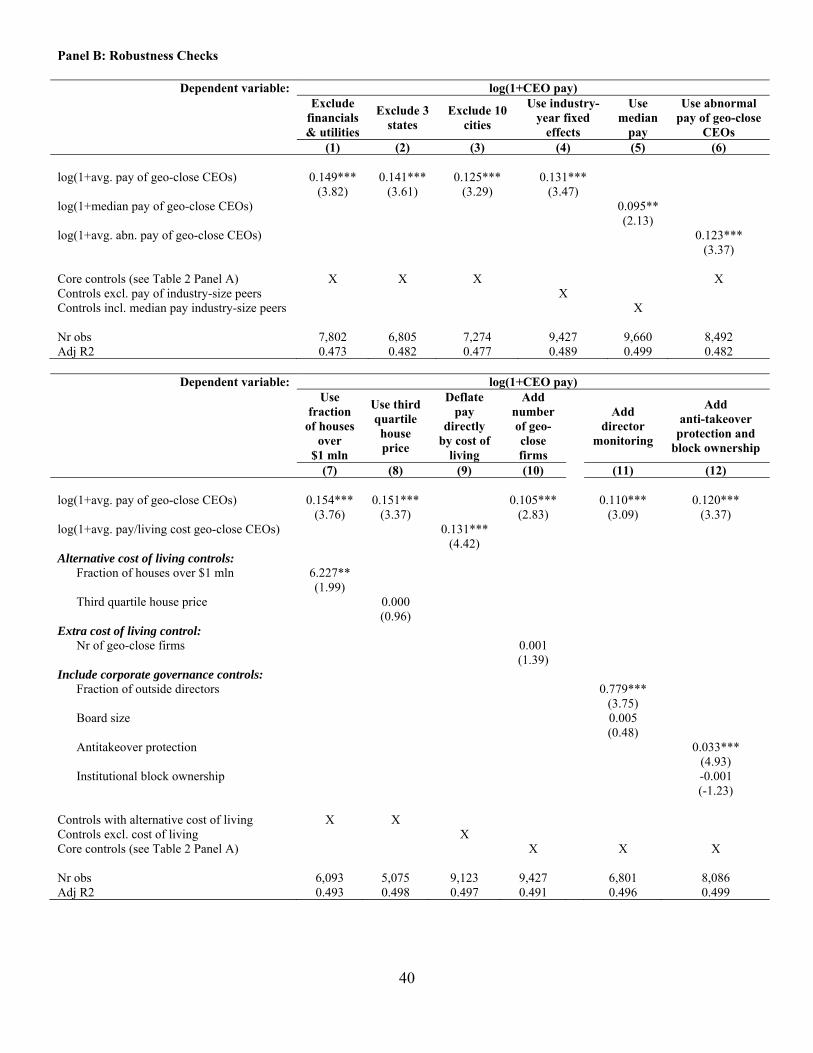
40
Panel B: Robustness Checks
Dependent variable: log(1+CEO pay)
Exclude
financials & utilities
Exclude 3 states
Exclude 10 cities
Use industry-year fixed
effects
Use median
pay
Use abnormal pay of geo-close
CEOs (1) (2) (3) (4) (5) (6)
log(1+avg. pay of geo-close CEOs) 0.149*** 0.141*** 0.125*** 0.131*** (3.82) (3.61) (3.29) (3.47) log(1+median pay of geo-close CEOs) 0.095** (2.13) log(1+avg. abn. pay of geo-close CEOs) 0.123*** (3.37) Core controls (see Table 2 Panel A) X X X X Controls excl. pay of industry-size peers X Controls incl. median pay industry-size peers X Nr obs 7,802 6,805 7,274 9,427 9,660 8,492 Adj R2 0.473 0.482 0.477 0.489 0.499 0.482
Dependent variable: log(1+CEO pay)
Use fraction
of houses over
$1 mln
Use third quartile house price
Deflate pay
directly by cost of
living
Add number of geo-close firms
Add
director monitoring
Add anti-takeover
protection and block ownership
(7) (8) (9) (10) (11) (12) log(1+avg. pay of geo-close CEOs) 0.154*** 0.151*** 0.105*** 0.110*** 0.120*** (3.76) (3.37) (2.83) (3.09) (3.37) log(1+avg. pay/living cost geo-close CEOs) 0.131*** (4.42) Alternative cost of living controls: Fraction of houses over $1 mln 6.227** (1.99) Third quartile house price 0.000 (0.96) Extra cost of living control: Nr of geo-close firms 0.001 (1.39) Include corporate governance controls: Fraction of outside directors 0.779*** (3.75) Board size 0.005 (0.48) Antitakeover protection 0.033*** (4.93) Institutional block ownership -0.001 (-1.23) Controls with alternative cost of living X X Controls excl. cost of living X Core controls (see Table 2 Panel A) X X X Nr obs 6,093 5,075 9,123 9,427 6,801 8,086 Adj R2 0.493 0.498 0.497 0.491 0.496 0.499
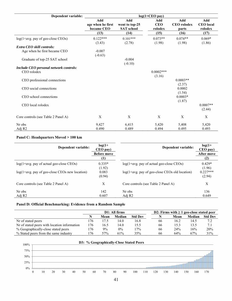
41
Dependent variable: log(1+CEO pay)
Add age when he first
became CEO
Add went to top-25
SAT school
Add CEO
rolodex
Add CEO rolodex
parts
Add CEO local
rolodex (13) (14) (15) (16) (17)
log(1+avg. pay of geo-close CEOs) 0.122*** 0.101*** 0.073** 0.074** 0.069* (3.43) (2.78) (1.98) (1.98) (1.86) Extra CEO skill controls: Age when he first became CEO -0.007 (-0.63) Graduate of top-25 SAT school -0.004 (-0.10) Include CEO personal network controls: CEO rolodex 0.0002*** (3.16) CEO professional connections 0.0003** (2.37) CEO social connections 0.0002 (1.54) CEO school connections 0.0003* (1.87) CEO local rolodex 0.0007** (2.44) Core controls (see Table 2 Panel A) X X X X X Nr obs 9,427 6,415 5,420 5,408 5,420 Adj R2 0.490 0.489 0.494 0.495 0.493 Panel C: Headquarters Moved > 100 km
Dependent variable: log(1+
CEO pay)
Dependent variable: log(1+
CEO pay) Before move After move (1) (2)
log(1+avg. pay of actual geo-close CEOs) 0.335* log(1+avg. pay of actual geo-close CEOs) 0.429* (1.92) (1.96) log(1+avg. pay of geo-close CEOs new location) 0.083 log(1+avg. pay of geo-close CEOs old location) 0.227*** (0.94) (2.94) Core controls (see Table 2 Panel A) X Core controls (see Table 2 Panel A) X Nr obs 142 Nr obs 136 Adj R2 0.607 Adj R2 0.649 Panel D: Official Benchmarking: Evidence from a Random Sample
D1: All firms D2: Firms with ≥ 1 geo-close stated peer N Mean Median Std Dev N Mean Median Std Dev Nr of stated peers 176 17.5 14.0 16.8 66 16.2 14.5 7.2 Nr of stated peers with location information 176 16.5 14.0 15.5 66 15.3 13.5 7.1 % Geographically-close stated peers 176 9% 0% 17% 66 24% 16% 20% % Stated peers from the same industry 176 57% 61% 35% 66 64% 67% 31%
0%
25%
50%
75%
100%
0 10 20 30 40 50 60 70 80 90 100 110 120 130 140 150 160 170
D3: % Geographically-Close Stated Peers
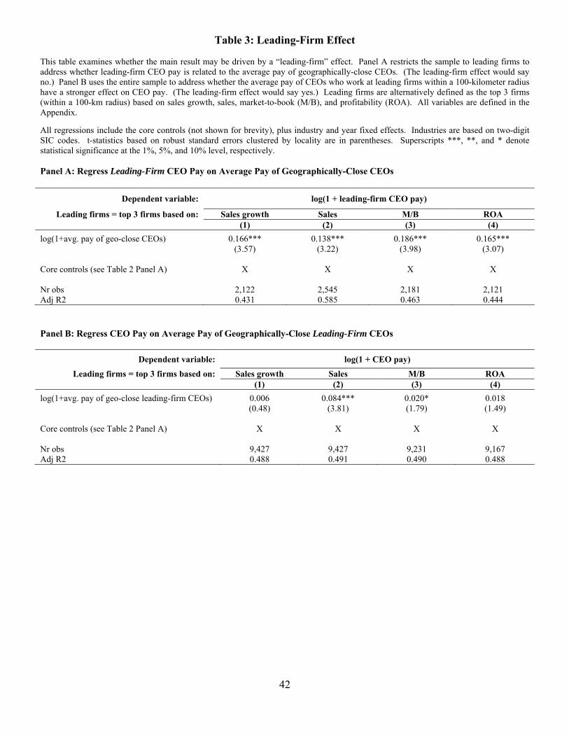
42
Table 3: Leading-Firm Effect This table examines whether the main result may be driven by a “leading-firm” effect. Panel A restricts the sample to leading firms to address whether leading-firm CEO pay is related to the average pay of geographically-close CEOs. (The leading-firm effect would say no.) Panel B uses the entire sample to address whether the average pay of CEOs who work at leading firms within a 100-kilometer radius have a stronger effect on CEO pay. (The leading-firm effect would say yes.) Leading firms are alternatively defined as the top 3 firms (within a 100-km radius) based on sales growth, sales, market-to-book (M/B), and profitability (ROA). All variables are defined in the Appendix.
All regressions include the core controls (not shown for brevity), plus industry and year fixed effects. Industries are based on two-digit SIC codes. t-statistics based on robust standard errors clustered by locality are in parentheses. Superscripts ***, **, and * denote statistical significance at the 1%, 5%, and 10% level, respectively. Panel A: Regress Leading-Firm CEO Pay on Average Pay of Geographically-Close CEOs
Dependent variable: log(1 + leading-firm CEO pay)
Leading firms = top 3 firms based on: Sales growth Sales M/B ROA (1) (2) (3) (4)
log(1+avg. pay of geo-close CEOs) 0.166*** 0.138*** 0.186*** 0.165*** (3.57) (3.22) (3.98) (3.07) Core controls (see Table 2 Panel A) X X X X Nr obs 2,122 2,545 2,181 2,121 Adj R2 0.431 0.585 0.463 0.444
Panel B: Regress CEO Pay on Average Pay of Geographically-Close Leading-Firm CEOs
Dependent variable: log(1 + CEO pay)
Leading firms = top 3 firms based on: Sales growth Sales M/B ROA (1) (2) (3) (4)
log(1+avg. pay of geo-close leading-firm CEOs) 0.006 0.084*** 0.020* 0.018 (0.48) (3.81) (1.79) (1.49) Core controls (see Table 2 Panel A) X X X X Nr obs 9,427 9,427 9,231 9,167 Adj R2 0.488 0.491 0.490 0.488

43
Table 4: Local Labor Market Competition for CEOs This table examines whether local labor market competition for CEOs can explain the main result. Panel A restricts the sample to companies that are part of the S&P500, arguing that if these firms’ CEO pay is significantly related to pay of geographically-close CEOs, it cannot be driven by local labor market competition since the market for the CEOs at these firms should be global or national rather than local. Panel B focuses on top executives (alternatively defined as non-CEO executives or the CFO), arguing that if local labor market competition drives the results, geography should also be related to compensation of these executives. All variables are defined in the Appendix. Regressions include control variables as indicated, plus industry and year fixed effects. Industries are based on two-digit SIC codes. t-statistics based on robust standard errors clustered by locality are in parentheses. Superscripts ***, **, and * denote statistical significance at the 1%, 5%, and 10% level, respectively. Panel A: Results for CEOs at S&P500 Firms
Dependent variable: log(1+CEO pay) (1) (2) log(1+avg. pay of geo-close CEOs) 0.116** 0.110* (2.09) (1.84) Core controls (see Table 2 Panel A) X Controls incl. avg. pay at S&P500 firms X Nr obs 3,099 2,835 Adj R2 0.378 0.403 Panel B: Results for Top Executives
Dependent variable: log(1+top exec pay) Non-CEO
executive CFO
(1) (2)
log(1+avg. pay of geo-close top execs) 0.002 -0.039 (0.07) (-1.19) Top exec pay controls (see main text) X X Nr obs 9,479 4,817 Adj R2 0.608 0.525

44
Table 5: Relative Status Concerns This table examines whether relative status concerns among CEOs can explain the main result. The percentage change in CEO pay is regressed on the CEO’s % pay gap plus control variables. Panel A shows the main result plus robustness tests. Panel B focuses on sports player evidence. CEO pay (salary) is regressed on the pay of geographically-close professional sports players (MLB, NBA, NFL, NHL, and the maximum of these), plus controls. All variables are defined in the Appendix. The regressions include control variables as indicated (not shown for brevity), plus industry and year fixed effects. Industries are based on two-digit SIC codes. t-statistics based on robust standard errors clustered by locality are in parentheses. Superscripts ***, **, and * denote statistical significance at the 1%, 5%, and 10% level, respectively. Panel A: Main Relative Status Concerns Results plus Robustness Tests
Dependent variable: %Δ CEO pay
Main: Pay gap based on
average pay
Pay gap based on
median pay
Positive pay gap interaction for
CEOs who are likely the most envious
(1) (2) (3)
% pay gap between (avg.) geo-close CEOs and CEO 0.083*** 0.003 (7.28) (0.25) % pay gap between (median) geo-close CEOs and CEO 0.057*** (8.57) % pay gap between (median) industry-size peers and CEO 0.176*** (10.90) % pay gap between (avg.) geo-close CEOs and CEO * (positive pay gap) 0.647*** (9.22) Relative status concerns core controls: % pay gap between (avg.) industry-size peers and CEO 0.191*** 0.163*** (11.57) (10.74) CEO age -0.401 -0.365 -0.143 (-1.65) (-1.49) (-0.56) CEO tenure -0.206 -0.239 -0.511* (-0.84) (-0.96) (-1.92) External CEO 4.772 4.664 2.297 (1.39) (1.36) (0.65) %Δ Firm size 0.130** 0.131** 0.134** (2.11) (2.13) (2.21) M/B ratio 4.198*** 4.462*** 4.692*** (3.67) (3.85) (3.93) Stock returns 1.052* 1.008* 0.918* (1.94) (1.86) (1.70) Δ Profitability 0.008 0.008 0.009 (1.42) (1.43) (1.61) Cost of living 0.010 0.034 -0.043 (0.17) (0.62) (-0.77) Per capita income 13.659** 14.931*** 13.158** (2.55) (2.71) (2.22) State income tax rate 60.486 68.145 48.716 (1.18) (1.30) (0.92) Constant -8.844 -15.883 -35.686 (-0.39) (-0.70) (-1.45) Nr obs 8,397 8,397 8,397 Adj R2 0.071 0.072 0.086

45
Panel B: Relative Status Concerns – Sports Player Evidence
Dependent variable: log(CEO salary)
Main
sample MLB NBA NFL NHL
Team maximum
(1) (2) (3) (4) (5) (6)
log(1+avg. salary of geo-close CEOs) 0.253*** (3.23) log(avg. salary of geo-close professional sports players identified in the table column) -0.015 0.146** 0.065** 0.051 0.097* (-0.49) (2.48) (2.35) (0.96) (1.67) Core controls (see Table 2 Panel A) X X X X X X Nr obs 9,427 6,923 3,232 3,850 2,876 7,402 Adj R2 0.282 0.331 0.291 0.303 0.280 0.284