the genetics package - university of...
TRANSCRIPT

The genetics PackageNovember 9, 2005
Title Population Genetics
Version 1.2.0
Date 2005-11-09
Author Gregory Warnes and Friedrich Leisch
Maintainer Gregory Warnes <[email protected]>
Depends combinat, gdata, MASS, mvtnorm
Description Classes and methods for handling genetic data. Includes classes to represent genotypesand haplotypes at single markers up to multiple markers on multiple chromosomes. Functioninclude allele frequencies, flagging homo/heterozygotes, flagging carriers of certain alleles,estimating and testing for Hardy-Weinberg disequilibrium, estimating and testing for linkagedisequilibrium, ...
License GPL
R topics documented:
HWE.chisq . . . . . . . . . . . . . . . . . . . . . . . . . . . . . . . . . . . . . . . . .2HWE.exact . . . . . . . . . . . . . . . . . . . . . . . . . . . . . . . . . . . . . . . . .3HWE.test . . . . . . . . . . . . . . . . . . . . . . . . . . . . . . . . . . . . . . . . . .4LD . . . . . . . . . . . . . . . . . . . . . . . . . . . . . . . . . . . . . . . . . . . . . .6binsearch . . . . . . . . . . . . . . . . . . . . . . . . . . . . . . . . . . . . . . . . . .8ci.balance . . . . . . . . . . . . . . . . . . . . . . . . . . . . . . . . . . . . . . . . . .10diseq . . . . . . . . . . . . . . . . . . . . . . . . . . . . . . . . . . . . . . . . . . . . .12expectedGenotypes . . . . . . . . . . . . . . . . . . . . . . . . . . . . . . . . . . . . .14genotype . . . . . . . . . . . . . . . . . . . . . . . . . . . . . . . . . . . . . . . . . . .15gregorius . . . . . . . . . . . . . . . . . . . . . . . . . . . . . . . . . . . . . . . . . .19homozygote . . . . . . . . . . . . . . . . . . . . . . . . . . . . . . . . . . . . . . . . .20locus . . . . . . . . . . . . . . . . . . . . . . . . . . . . . . . . . . . . . . . . . . . . .22makeGenotypes . . . . . . . . . . . . . . . . . . . . . . . . . . . . . . . . . . . . . . .25plot.genotype . . . . . . . . . . . . . . . . . . . . . . . . . . . . . . . . . . . . . . . .27power.casectrl . . . . . . . . . . . . . . . . . . . . . . . . . . . . . . . . . . . . . . . .28print.LD . . . . . . . . . . . . . . . . . . . . . . . . . . . . . . . . . . . . . . . . . . .29summary.genotype . . . . . . . . . . . . . . . . . . . . . . . . . . . . . . . . . . . . .31undocumented . . . . . . . . . . . . . . . . . . . . . . . . . . . . . . . . . . . . . . . .33write.pop.file . . . . . . . . . . . . . . . . . . . . . . . . . . . . . . . . . . . . . . . .33
Index 35
1

2 HWE.chisq
HWE.chisq Perform Chi-Square Test for Hardy-Weinberg Equilibrium
Description
Test the null hypothesis that Hardy-Weinberg equilibrium holds using the Chi-Square method.
Usage
HWE.chisq(x, ...)## S3 method for class 'genotype':HWE.chisq(x, simulate.p.value=TRUE, B=10000, ...)
Arguments
x genotype or haplotype object.simulate.p.value
a logical value indicating whether the p-value should be computed using simu-lation instead of using theχ2 approximation. Defaults toTRUE.
B Number of simulation iterations to use whensimulate.p.value=TRUE .Defaults to 10000.
... optional parameters passed tochisq.test
Details
This function generates a 2-way table of allele counts, then callschisq.test to compute a p-value for Hardy-Weinberg Equilibrium. By default, it uses an unadjusted Chi-Square test statisticand computes the p-value using a simulation/permutation method. Whensimulate.p.value=FALSE ,it computes the test statistic using the Yates continuity correction and tests it against the asymptoticChi-Square distribution with the approproate degrees of freedom.
Note: The Yates continuty correction is applied *only* whensimulate.p.value=FALSE , sothat the reported test statistics whensimulate.p.value=FALSE andsimulate.p.value=TRUEwill differ.
Value
An object of classhtest .
See Also
HWE.exact , HWE.test , diseq , diseq.ci , allele , chisq.test , boot , bootci
Examples
example.data <- c("D/D","D/I","D/D","I/I","D/D","D/D","D/D","D/D","I/I","")
g1 <- genotype(example.data)g1

HWE.exact 3
HWE.chisq(g1)# compare withHWE.exact(g1)# andHWE.test(g1)
three.data <- c(rep("A/A",8),rep("C/A",20),rep("C/T",20),rep("C/C",10),rep("T/T",3))
g3 <- genotype(three.data)g3
HWE.chisq(g3, B=10000)
HWE.exact Exact Test of Hardy-Weinberg Equilibrium for 2-Allele Markers
Description
Exact test of Hardy-Weinberg Equilibrium for 2 Allele Markers.
Usage
HWE.exact(x)
Arguments
x Genotype object
Value
Object of class ’htest’.
Note
This function only works for genotypes with exactly 2 alleles.
Author(s)
David Duffy 〈[email protected]〉 with modifications by Gregory R. Warnes〈[email protected]〉
References
Emigh TH. (1980) "Comparison of tests for Hardy-Weinberg Equilibrium", Biometrics, 36, 627-642.
See Also
HWE.chisq , HWE.test , diseq , diseq.ci

4 HWE.test
Examples
example.data <- c("D/D","D/I","D/D","I/I","D/D","D/D","D/D","D/D","I/I","")
g1 <- genotype(example.data)g1
HWE.exact(g1)# compare withHWE.chisq(g1)
g2 <- genotype(sample( c("A","C"), 100, p=c(100,10), rep=TRUE),sample( c("A","C"), 100, p=c(100,10), rep=TRUE) )
HWE.exact(g2)
HWE.test Estimate Disequilibrium and Test for Hardy-Weinberg Equilibrium
Description
Estimate disequilibrium parameter and test the null hypothesis that Hardy-Weinberg equilibriumholds.
Usage
HWE.test(x, ...)## S3 method for class 'genotype':HWE.test(x, exact = nallele(x)==2, simulate.p.value=!exact,
B=10000, conf=0.95, ci.B=1000, ... )## S3 method for class 'data.frame':HWE.test(x, ..., do.Allele.Freq=TRUE, do.HWE.test=TRUE)## S3 method for class 'HWE.test':print(x, show=c("D","D'","r"), ...)
Arguments
x genotype or haplotype object.
exact a logical value indicated whether the p-value should be computed using the exactmethod, which is only available for 2 allele genotypes.
simulate.p.valuea logical value indicating whether the p-value should be computed using simu-lation instead of using theχ2 approximation. Defaults toTRUE.
B Number of simulation iterations to use whensimulate.p.value=TRUE .Defaults to 10000.
conf Confidence level to use when computing the confidence level for D-hat. Defaultsto 0.95, should be in (0,1).
ci.B Number of bootstrap iterations to use when computing the confidence interval.Defaults to 1000.

HWE.test 5
show a character vector containing the names of HWE test statistics to display fromthe set of "D", "D’", and "r".
... optional parameters passed toHWE.test (data.frame method) orchisq.test(base method).
do.Allele.Freqlogicial indication whether to summarize allele frequencies.
do.HWE.test logicial indication whether to perform HWE tests
Details
HWE.test callsdiseq to computes the Hardy-Weinberg (dis)equilibrium statistics D, D’, and r(correlation coefficient). Next it callsdiseq.ci to compute a bootstrap confidence interval forthese estimates. Finally, it callschisq.test to compute a p-value for Hardy-Weinberg Equilib-rium using a simulation/permutation method.
Using bootstrapping for the confidence interval and simulation for the p-value avoids reliance on theassumptions the underlying Chi-square approximation. This is particularly important when someallele pairs have small counts.
For details on the definition of D, D’, and r, see the help page fordiseq .
Value
An object of classHWE.test with components
diseq A diseq object providing details on the disequilibrium estimates.
ci A diseq.ci object providing details on the bootstrap confidence intervals forthe disequilibrium estimates.
test A htest object providing details on the permutation based Chi-square test.
call function call used to creat this object.conf, B, ci.B, simulate.p.value
values used for these arguments.
Author(s)
Gregory R. Warnes〈[email protected]〉
See Also
genotype , diseq , diseq.ci , HWE.chisq , HWE.exact ,
Examples
example.data <- c("D/D","D/I","D/D","I/I","D/D","D/D","D/D","D/D","I/I","")
g1 <- genotype(example.data)g1
HWE.test(g1)
#compare withdiseq(g1)diseq.ci(g1)

6 LD
HWE.chisq(g1)HWE.exact(g1)
three.data <- c(rep("A/A",8),rep("C/A",20),rep("C/T",20),rep("C/C",10),rep("T/T",3))
g3 <- genotype(three.data)g3
HWE.test(g3, ci.B=10000)
LD Pairwise linkage disequilibrium between genetic markers.
Description
Compute pairwise linkage disequilibrium between genetic markers
Usage
LD(g1, ...)## S3 method for class 'genotype':LD(g1,g2,...)## S3 method for class 'data.frame':LD(g1,...)
Arguments
g1 genotype object or dataframe containing genotype objects
g2 genotype object (ignored if g1 is a dataframe)
... optional arguments (ignored)
Details
Linkage disequilibrium (LD) is the non-random association of marker alleles and can arise frommarker proximity or from selection bias.
LD.genotype estimates the extent of LD for a single pair of genotypes.LD.data.frame com-putes LD for all pairs of genotypes contained in a data frame. Before starting,LD.data.framechecks the class and number of alleles of each variable in the dataframe. If the data frame containsnon-genotype objects or genotypes with more or less than 2 alleles, these will be omitted from thecomputation and a warning will be generated.
Three estimators of LD are computed:
D raw difference in frequency between the observed number of AB pairs and the expected num-ber:
D = pAB − pApB
LD 7
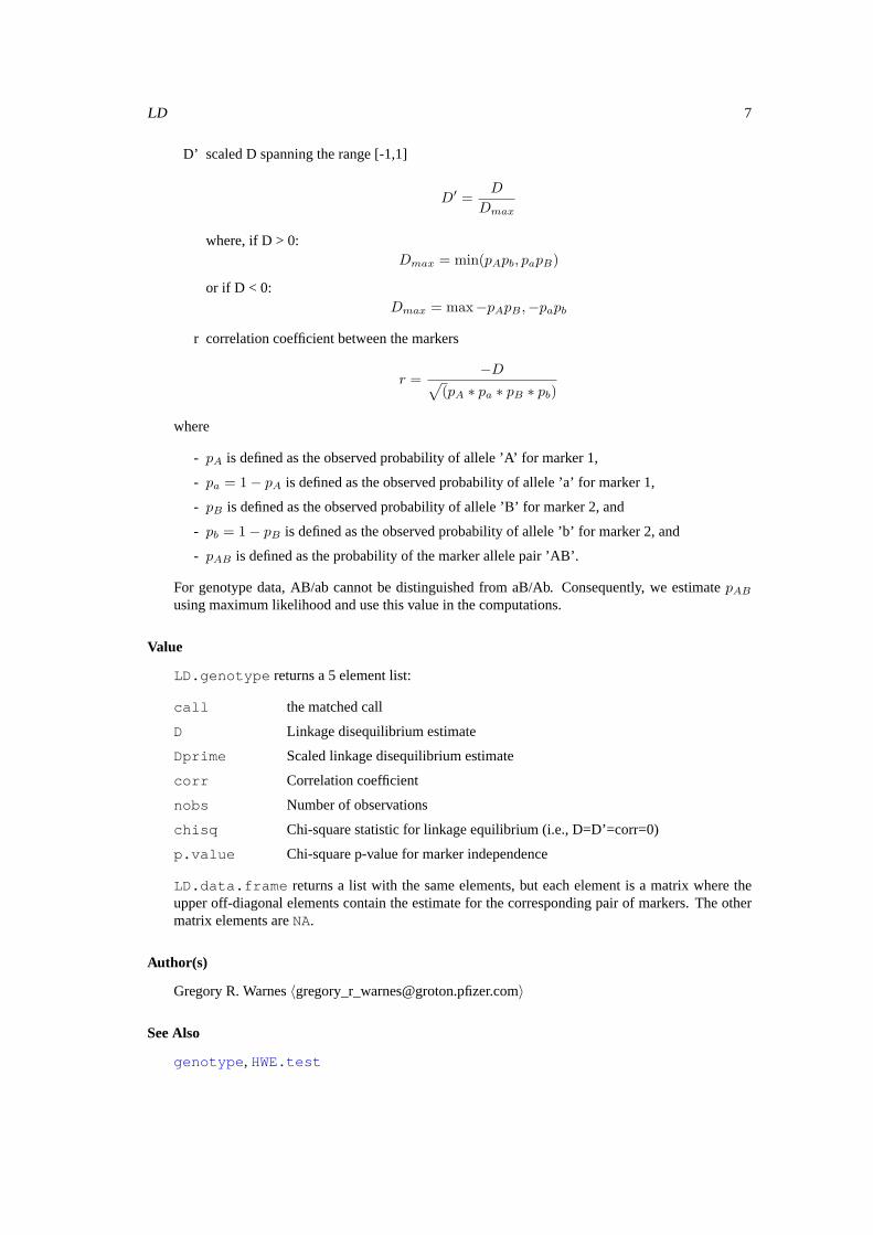
D’ scaled D spanning the range [-1,1]
D′ =D
Dmax
where, if D > 0:Dmax = min(pApb, papB)
or if D < 0:Dmax = max−pApB ,−papb
r correlation coefficient between the markers
r =−D√
(pA ∗ pa ∗ pB ∗ pb)
where
- pA is defined as the observed probability of allele ’A’ for marker 1,
- pa = 1 − pA is defined as the observed probability of allele ’a’ for marker 1,
- pB is defined as the observed probability of allele ’B’ for marker 2, and
- pb = 1 − pB is defined as the observed probability of allele ’b’ for marker 2, and
- pAB is defined as the probability of the marker allele pair ’AB’.
For genotype data, AB/ab cannot be distinguished from aB/Ab. Consequently, we estimatepAB
using maximum likelihood and use this value in the computations.
Value
LD.genotype returns a 5 element list:
call the matched call
D Linkage disequilibrium estimate
Dprime Scaled linkage disequilibrium estimate
corr Correlation coefficient
nobs Number of observations
chisq Chi-square statistic for linkage equilibrium (i.e., D=D’=corr=0)
p.value Chi-square p-value for marker independence
LD.data.frame returns a list with the same elements, but each element is a matrix where theupper off-diagonal elements contain the estimate for the corresponding pair of markers. The othermatrix elements areNA.
Author(s)
Gregory R. Warnes〈[email protected]〉
See Also
genotype , HWE.test

8 binsearch
Examples
g1 <- genotype( c('T/A', NA, 'T/T', NA, 'T/A', NA, 'T/T', 'T/A','T/T', 'T/T', 'T/A', 'A/A', 'T/T', 'T/A', 'T/A', 'T/T',
NA, 'T/A', 'T/A', NA) )
g2 <- genotype( c('C/A', 'C/A', 'C/C', 'C/A', 'C/C', 'C/A', 'C/A', 'C/A','C/A', 'C/C', 'C/A', 'A/A', 'C/A', 'A/A', 'C/A', 'C/C','C/A', 'C/A', 'C/A', 'A/A') )
g3 <- genotype( c('T/A', 'T/A', 'T/T', 'T/A', 'T/T', 'T/A', 'T/A', 'T/A','T/A', 'T/T', 'T/A', 'T/T', 'T/A', 'T/A', 'T/A', 'T/T','T/A', 'T/A', 'T/A', 'T/T') )
# Compute LD on a single pair
LD(g1,g2)
# Compute LD table for all 3 genotypes
data <- makeGenotypes(data.frame(g1,g2,g3))LD(data)
binsearch Binary Search
Description
Search within a specified range to locate an integer parameter which results in the the specifiedmonotonic function obtaining a given value.
Usage
binsearch(fun, range, ..., target = 0, lower = ceiling(min(range)),upper = floor(max(range)), maxiter = 100, showiter = FALSE)
Arguments
fun Monotonic function over which the search will be performed.
range 2-element vector giving the range for the search.
... Additional parameters to the functionfun .
target Target value forfun . Defaults to 0.
lower Lower limit of search range. Defaults tomin(range) .
upper Upper limit of search range. Defaults tomax(range) .
maxiter Maximum number of search iterations. Defaults to 100.
showiter Boolean flag indicating whether the algorithm state should be printed at eachiteration. Defaults to FALSE.

binsearch 9
Details
This function implements an extension to the standard binary search algorithm for searching a sortedlist. The algorithm has been extended to cope with cases where an exact match is not possible, todetect whether that the function may be monotonic increasing or decreasing and act appropriately,and to detect when the target value is outside the specified range.
The algorithm initializes two variablelo and high to the extremes values ofrange . It thengenerates a new valuecenter halfway betweenlo and hi . If the value offun at centerexceedstarget , it becomes the new value forlo , otherwise it becomes the new value forhi .This process is iterated untillo andhi are adjacent. If the function at one or the other equals thetarget, this value is returned, otherwiselo , hi , and the function value at both are returned.
Note that when the specified target value falls between integers, thetwo closest values are returned.If the specified target falls outside of the specifiedrange , the closest endpoint of the range willbe returned, and an warning message will be generated. If the maximum number if iterations wasreached, the endpoints of the current subset of the range under consideration will be returned.
Value
A list containing:
call How the function was called.
numiter The number of iterations performed
flag One of the strings, "Found", "Between Elements", "Maximum number of itera-tions reached", "Reached lower boundary", or "Reached upper boundary."
where One or two values indicating where the search terminated.
value Value of the functionfun at the values ofwhere .
Note
This function often returns two values forwhere andvalue . Be sure to check theflag parameterto see what these values mean.
Author(s)
Gregory R. Warnes〈[email protected]〉
See Also
optim , optimize , uniroot
Examples
### Toy examples
# search for x=10binsearch( function(x) x-10, range=c(0,20) )
# search for x=10.1binsearch( function(x) x-10.1, range=c(0,20) )
### Classical toy example

10 ci.balance
# binary search for the index of 'M' among the sorted lettersfun <- function(X) ifelse(LETTERS[X] > 'M', 1,
ifelse(LETTERS[X] < 'M', -1, 0 ) )
binsearch( fun, range=1:26 )# returns $where=13LETTERS[13]
### Substantive example, from genetics
# Determine the necessary sample size to detect all alleles with# frequency 0.07 or greater with probability 0.95.power.fun <- function(N) 1 - gregorius(N=N, freq=0.07)$missprob
binsearch( power.fun, range=c(0,100), target=0.95 )
# equivalent togregorius( freq=0.07, missprob=0.05)
ci.balance Experimental Function to Correct Confidence Intervals At or NearBoundaries of the Parameter Space by ’Sliding’ the Interval on theQuantile Scale.
Description
Experimental function to correct confidence intervals at or near boundaries of the parameter spaceby ’sliding’ the interval on the quantile scale.
Usage
ci.balance(x, est, confidence=0.95, alpha=1-confidence, minval, maxval,na.rm=TRUE)
Arguments
x Bootstrap parameter estimates.
est Observed value of the parameter.
confidence Confidence level for the interval. Defaults to 0.95.
alpha Type I error rate (size) for the interval. Defaults to 1-confidence .
minval A numeric value specifying the lower bound of the parameter space. Leaveunspecified (the default) if there is no lower bound.
maxval A numeric value specifying the upper bound of the parameter space. Leaveunspecified (the default) if there is no upper bound.
na.rm logical. Should missing values be removed?
ci.balance 11
Details
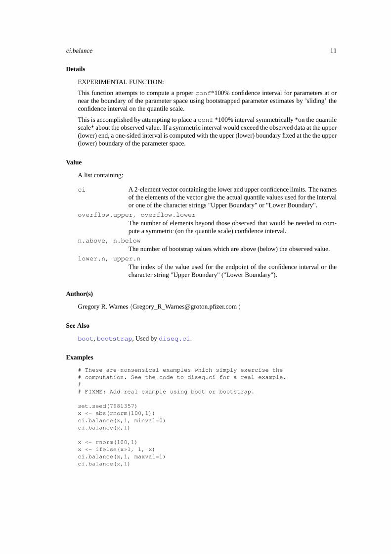
EXPERIMENTAL FUNCTION:
This function attempts to compute a properconf *100% confidence interval for parameters at ornear the boundary of the parameter space using bootstrapped parameter estimates by ’sliding’ theconfidence interval on the quantile scale.
This is accomplished by attempting to place aconf *100% interval symmetrically *on the quantilescale* about the observed value. If a symmetric interval would exceed the observed data at the upper(lower) end, a one-sided interval is computed with the upper (lower) boundary fixed at the the upper(lower) boundary of the parameter space.
Value
A list containing:
ci A 2-element vector containing the lower and upper confidence limits. The namesof the elements of the vector give the actual quantile values used for the intervalor one of the character strings "Upper Boundary" or "Lower Boundary".
overflow.upper, overflow.lowerThe number of elements beyond those observed that would be needed to com-pute a symmetric (on the quantile scale) confidence interval.
n.above, n.belowThe number of bootstrap values which are above (below) the observed value.
lower.n, upper.nThe index of the value used for the endpoint of the confidence interval or thecharacter string "Upper Boundary" ("Lower Boundary").
Author(s)
Gregory R. Warnes〈[email protected]〉
See Also
boot , bootstrap , Used bydiseq.ci .
Examples
# These are nonsensical examples which simply exercise the# computation. See the code to diseq.ci for a real example.## FIXME: Add real example using boot or bootstrap.
set.seed(7981357)x <- abs(rnorm(100,1))ci.balance(x,1, minval=0)ci.balance(x,1)
x <- rnorm(100,1)x <- ifelse(x>1, 1, x)ci.balance(x,1, maxval=1)ci.balance(x,1)

12 diseq
diseq Estimate or Compute Confidence Interval for the Single-Marker Dise-quilibrium
Description
Estimate or compute confidence interval for single-marker disequilibrium.
Usage
diseq(x, ...)## S3 method for class 'diseq':print(x, show=c("D","D'","r","R^2","table"), ...)diseq.ci(x, R=1000, conf=0.95, correct=TRUE, na.rm=TRUE, ...)
Arguments
x genotype or haplotype object.
show a character value or vector indicating which disequilibrium measures should bedisplayed. The default is to show all of the available measures.show="table"will display a table of observed, expected, and observed-expected frequencies.
conf Confidence level to use when computing the confidence level for D-hat. Defaultsto 0.95, should be in (0,1).
R Number of bootstrap iterations to use when computing the confidence interval.Defaults to 1000.
correct See details.
na.rm logical. Should missing values be removed?
... optional parameters passed toboot.ci (diseq.ci ) or ignored.
Details
For a single-gene marker,diseq computes the Hardy-Weinberg (dis)equilibrium statistic D, D’,r (the correlation coefficient), andr2 for each pair of allele values, as well as an overall summaryvalue for each measure across all alleles.print.diseq displays the contents of adiseq object.diseq.ci computes a bootstrap confidence interval for this estimate.
For consistency, I have applied the standard definitions for D, D’, and r from the Linkage Disequi-librium case, replacing all marker probabilities with the appropriate allele probabilities.
Thus, for each allele pair,
D is defined as the half of the raw difference in frequency between the observed number ofheterozygotes and the expected number:
D =12(pij + pji) − pipj
D’ rescales D to span the range [-1,1]
D′ =D
Dmax

diseq 13
where, if D > 0:
Dmax = min pipj , pjpi = pipj
or if D < 0:
Dmax = min pi(1 − pj), pj(1 − pi)
r is the correlation coefficient between two alleles, and can be computed by
r =−D√
(pi ∗ (1 − pi)p(j)(1 − pj))
where
- pi defined as the observed probability of allele ’i’,
- pj defined as the observed probability of allele ’j’, and
- pij defined as the observed probability of the allele pair ’ij’.
When there are more than two alleles, the summary values for these statistics are obtained by com-puting a weighted average of the absolute value of each allele pair, where the weight is determinedby the expected frequency. For example:
Doverall =∑i 6=j
|Dij | ∗ pij
Bootstrapping is used to generate confidence interval in order to avoid reliance on parametric as-sumptions, which will not hold for alleles with low frequencies (e.g.D′ following a a Chi-squaredistribution).
See the functionHWE.test for testing Hardy-Weinberg Equilibrium,D = 0.
Value
diseq returns an object of classdiseq with components
data 2-way table of allele pair counts
D.hat matrix giving the observed count, expected count, observed - expected differ-ence, and estimate of disequilibrium for each pair of alleles as well as an overalldisequilibrium value.
call function call used to create this object
normal-bracket98bracket-normal
diseq.ci returns an object of classbootci
Author(s)
Gregory R. Warnes〈[email protected]〉
See Also
genotype , HWE.test , boot , bootci

14 expectedGenotypes
Examples
example.data <- c("D/D","D/I","D/D","I/I","D/D","D/D","D/D","D/D","I/I","")
g1 <- genotype(example.data)g1
diseq(g1)diseq.ci(g1)HWE.test(g1) # does the same, plus tests D-hat=0
three.data <- c(rep("A/A",8),rep("C/A",20),rep("C/T",20),rep("C/C",10),rep("T/T",3))
g3 <- genotype(three.data)g3
diseq(g3)diseq.ci(g3, ci.B=10000, ci.type="bca")
# only show observed vs expected tableprint(diseq(g3),show='table')
expectedGenotypes Construct expected genotypes according to known allele variants
Description
expectedGenotypes constructs expected genotypes according to known allele variants, whichcan be quite tedious with large number of allele variants. It can handle data with different level ofploidy.
Usage
expectedGenotypes(x, alleles = allele.names(x), ploidy = 2)
Arguments
x genotype object, as genotype.
alleles vector of allele names, as character.
ploidy number of chromosome sets i.e. 2 for human autosomal genes, as integer.
At least one ofx or alleles must be given.
Value
A character vector with genotype names as "alele1/alele2" for diploid example.

genotype 15
Author(s)
Gregor GORJANC
See Also
allele.names , genotype
Examples
## Not run: Scrapie example
scrapie <- c("ARQ/ARQ", "ARQ/ARQ", "ARR/ARQ", "AHQ/ARQ", "ARQ/ARQ")expectedGenotypes(as.genotype(scrapie))expectedGenotypes(alleles=c("ARR", "AHQ", "ARH", "ARQ", "VRR", "VRQ"))scrapie <- genotype(scrapie,
alleles=c("ARR", "AHQ", "ARH", "ARQ", "VRR", "VRQ"),reorder="yes")
expectedGenotypes(scrapie)
genotype Genotype or Haplotype Objects.
Description
genotype creates a genotype object.
haplotype creates a haplotype object.
is.genotype returnsTRUEif x is of classgenotype
is.haplotype returnsTRUEif x is of classhaplotype
as.genotype attempts to coerce its argument into an object of classgenotype .
as.genotype.allele.count converts allele counts (0,1,2) into genotype pairs ("A/A", "A/B","B/B").
as.haplotype attempts to coerce its argument into an object of classhaplotype .
nallele returns the number of alleles in an object of classgenotype .
Usage
genotype(a1, a2=NULL, alleles=NULL, sep="/", remove.spaces=TRUE,reorder = c("yes", "no", "default", "ascii", "freq"),allow.partial.missing=FALSE, locus=NULL)
haplotype(a1, a2=NULL, alleles=NULL, sep="/", remove.spaces=TRUE,reorder="no", allow.partial.missing=FALSE, locus=NULL)
is.genotype(x)
is.haplotype(x)
as.genotype(x, ...)

16 genotype
as.genotype.allele.count(x, alleles=c("A","B"), ... )
as.haplotype(x, ...)
print.genotype(x, ...)
nallele(x)
Arguments
x either an object of classgenotype orhaplotype or an object to be convertedto classgenotype or haplotype .
a1,a2 vector(s) or matrix containing two alleles for each individual. See details, below.
alleles names (and order ifreorder="yes" ) of possible alleles.
sep character separator or column number used to divide alleles whena1 is a vectorof strings where each string holds both alleles. See below for details.
remove.spaceslogical indicating whether spaces and tabs will be removed from a1 and a2 be-fore processing.
reorder how should alleles within an individual be reordered. Ifreorder="no" ,use the order specified by the alleles parameter. Ifreorder="freq" orreorder="yes" , sort alleles within each individual by observed frequency.If reorder="ascii" , reorder alleles in ASCII order (alphabetical, with allupper case before lower case). The default value forgenotype is "freq" .The default value forhaplotype is "no" .
allow.partial.missinglogical indicating whether one allele is permitted to be missing. When set toFALSEboth alleles are set toNAwhen either is missing.
locus object of class locus, gene, or marker, holding information about the source ofthis genotype.
... optional arguments
Details
Genotype objects hold information on which gene or marker alleles were observed for differentindividuals. For each individual, two alleles are recorded.
The genotype class considers the stored alleles to be unordered, i.e., "C/T" is equivalent to "T/C".The haplotype class considers the order of the alleles to be significant so that "C/T" is distinct from"T/C".
When callinggenotype or haplotype :
• If only a1 is provided and is a character vector, it is assumed that each element encodesboth alleles. In this case, ifsep is a character string,a1 is assumed to be coded as "Al-lele1<sep>Allele2". Ifsep is a numeric value, it is assumed that character locations1:sepcontain allele 1 and that remaining locations contain allele 2.
• If a1 is a matrix, it is assumed that column 1 contains allele 1 and column 2 contains allele 2.
• If a1 anda2 are both provided, each is assumed to contain one allele value so that the geno-type for an individual is obtained bypaste(a1,a2,sep="/") .

genotype 17
If remove.spaces is TRUE, (the default) any whitespace contained ina1 anda2 is removedwhen the genotypes are created. If whitespace is used as the separator, (eg "C C", "C T", ...), besure to set remove.spaces to FALSE.
When the alleles are explicitly specified using thealleles argument, all potential alleles notpresent in the list will be converted toNA.
NOTE: genotype assumes that the order of the alleles is not important (E.G., "A/C" == "C/A").Use classhaplotype if order is significant.
Value
The genotype class extends "factor" and haplotype extends genotype. Both classes have the follow-ing attributes:
levels character vector of possible genotype/haplotype values stored coded bypaste(allele1, "/", allele2, sep="") .
allele.names character vector of possible alleles. For a SNP, these might be c("A","T"). For avariable length dinucleotyde repeat this might be c("136","138","140","148").
allele.map matrix encoding how the factor levels correspond to alleles. See the source codeto allele.genotype() for how to extract allele values using this matrix.Better yet, just useallele.genotype() .
Author(s)
Gregory R. Warnes〈[email protected]〉 and Friedrich Leisch.
See Also
HWE.test , allele , homozygote , heterozygote , carrier , summary.genotype , allele.countlocus gene marker
Examples
# several examples of genotype data in different formatsexample.data <- c("D/D","D/I","D/D","I/I","D/D",
"D/D","D/D","D/D","I/I","")g1 <- genotype(example.data)g1
example.data2 <- c("C-C","C-T","C-C","T-T","C-C","C-C","C-C","C-C","T-T","")
g2 <- genotype(example.data2,sep="-")g2
example.nosep <- c("DD", "DI", "DD", "II", "DD","DD", "DD", "DD", "II", "")
g3 <- genotype(example.nosep,sep="")g3
example.a1 <- c("D", "D", "D", "I", "D", "D", "D", "D", "I", "")example.a2 <- c("D", "I", "D", "I", "D", "D", "D", "D", "I", "")g4 <- genotype(example.a1,example.a2)g4
example.mat <- cbind(a1=example.a1, a1=example.a2)

18 genotype
g5 <- genotype(example.mat)g5
example.data5 <- c("D / D","D / I","D / D","I / I","D / D","D / D","D / D","D / D","I / I","")
g5 <- genotype(example.data5,rem=TRUE)g5
# show how genotype and haplotype differdata1 <- c("C/C", "C/T", "T/C")data2 <- c("C/C", "T/C", "T/C")
test1 <- genotype( data1 )test2 <- genotype( data2 )
test3 <- haplotype( data1 )test4 <- haplotype( data2 )
test1==test2test3==test4
test1=="C/T"test1=="T/C"
test3=="C/T"test3=="T/C"
## "Messy" example
m3 <- c("D D/\t D D","D\tD/ I", "D D/ D D","I/ I","D D/ D D","D D/ D D","D D/ D D","D D/ D D","I/ I","/ ","/I")
genotype(m3)summary(genotype(m3))
m4 <- c("D D","D I","D D","I I","D D","D D","D D","D D","I I"," "," I")
genotype(m4,sep=1)genotype(m4,sep=" ",remove.spaces=FALSE)summary(genotype(m4,sep=" ",remove.spaces=FALSE))
m5 <- c("DD","DI","DD","II","DD","DD","DD","DD","II"," "," I")
genotype(m5,sep=1)haplotype(m5,sep=1,remove.spaces=FALSE)
g5 <- genotype(m5,sep="")h5 <- haplotype(m5,sep="")
heterozygote(g5)homozygote(g5)carrier(g5,"D")

gregorius 19
g5[9:10] <- haplotype(m4,sep=" ",remove=FALSE)[1:2]g5
g5[9:10]allele(g5[9:10],1)allele(g5,1)[9:10]
# drop unused allelesg5[9:10,drop=TRUE]h5[9:10,drop=TRUE]
# Convert allele.counts into genotype
x <- c(0,1,2,1,1,2,NA,1,2,1,2,2,2)g <- as.genotype.allele.count(x, alleles=c("C","T") )g
gregorius Probability of Observing All Alleles with a Given Frequency in a Sam-ple of a Specified Size.
Description
Probability of observing all alleles with a given frequency in a sample of a specified size.
Usage
gregorius(freq, N, missprob, tol = 1e-10, maxN = 10000, maxiter=100, showiter = FALSE)
Arguments
freq (Minimum) Allele frequency (required)
N Number of sampled genotypes
missprob Desired maximum probability of failing to observe an allele.
tol Omit computation for terms which contribute less than this value.
maxN Largest value to consider when searching for N.
maxiter Maximum number of iterations to use when searching for N.
showiter Boolean flag indicating whether to show the iterations performed when search-ing for N.
Details
If freq andN are provided, butmissprob is omitted, this function computes the probability offailing to observe all alleles with true underlying frequencyfreq whenN diploid genotypes aresampled. This is accomplished using the sum provided in Corollary 2 of Gregorius (1980), omittingterms which contribute less thantol to the result.
When freq and missprob are provide, butN is omitted. A binary search on the range of[1,maxN] is performed to locate the smallest sample size,N, for which the probability of failingto observe all alleles with true underlying frequencyfreq is at mostmissprob . In this case,maxiter specifies the largest number of iterations to use in the binary search, andshowitercontrols whether the iterations of the search are displayed.

20 homozygote
Value
A list containing the following values:
call Function call used to generate this object.
method One of the strings, "Compute missprob given N and freq", or "Determine min-imal N given missprob and freq", indicating which type of computation wasperformed.
retval$freq Specified allele frequency.
retval$N Specified or computed sample size.
retval$missprobComputed probability of failing to observe all of the alleles with frequencyfreq .
Note
This code produces sample sizes that are slightly larger than those given in table 1 of Gregorius(1980). This appears to be due to rounding of the computedmissprob s by the authors of thatpaper.
Author(s)
Code submitted by David Duffy〈[email protected]〉, substantially enhanced by Gregory R.Warnes〈[email protected]〉.
References
Gregorius, H.R. 1980. The probability of losing an allele when diploid genotypes are sampled.Biometrics 36, 643-652.
Examples
# Compute the probability of missing an allele with frequency 0.15 when# 20 genotypes are sampled:gregorius(freq=0.15, N=20)
# Determine what sample size is required to observe all alleles with true# frequency 0.15 with probability 0.95gregorius(freq=0.15, missprob=1-0.95)
homozygote Extract Features of Genotype objects

homozygote 21
Description
homozygote creates an vector of logicals that are true when the alleles of the correspondingobservation are the identical.
heterozygote creates an vector of logicals that are true when the alleles of the correspondingobservation differ.
carrier create a logical vector or matrix of logicals indicating whether the specified alleles arepresent.
allele.count returns the number of copies of the specified alleles carried by each observation.
allele extract the specified allele(s) as a character vector or a 2 column matrix.
allele.names extract the set of allele names.
Usage
homozygote(x, allele.name, ...)heterozygote(x, allele.name, ...)carrier(x, allele.name, ...)## S3 method for class 'genotype':carrier(x, allele.name=allele.names(x),
any=!missing(allele.name), na.rm=FALSE, ...)allele.count(x, allele.name=allele.names(x),any=!missing(allele.name),
na.rm=FALSE)allele(x, which=c(1,2) )allele.names(x)
Arguments
x genotype object
... optional parameters (ignored)
allele.name character value or vector of allele names
any logical value. WhenTRUE, a single count or indicator is returned by combiningthe results for all of the elements ofallele . If FALSE separate counts orindicators should be returned for each element ofallele . Defaults toFALSEif allele is missing. Otherwise defaults toTRUE.
na.rm logical value indicating whether to remove missing values. When true, anyNAvalues will be replaced by0 or FALSEas appropriate. Defaults toFALSE.
which selects which allele to return. For first allele use1. For second allele use2. Forboth (the default) usec(1,2) .
Details
When theallele.name argument is given, heterozygote and homozygote returnTRUEif exactlyone or both alleles, respectively, match the specified allele.name.
Value
homozygote andheterozygote return a vector of logicals.
carrier returns a logical vector if only one allele is specified, or ifany is TRUE. Otherwise, itreturns matrix of logicals with one row for each element ofallele .

22 locus
allele.count returns a vector of counts if only one allele is specified, or ifany is TRUE.Otherwise, it returns matrix of counts with one row for each element ofallele .
allele returns a character vector when one allele is specified. When 2 alleles are specified, itreturns a 2 column character matrix.
allele.names returns a character vector containing the set of allele names.
Author(s)
Gregory R. Warnes〈[email protected]〉
See Also
genotype , HWE.test , summary.genotype , locus gene marker
Examples
example.data <- c("D/D","D/I","D/D","I/I","D/D","D/D","D/D","D/D","I/I","")g1 <- genotype(example.data)g1
heterozygote(g1)homozygote(g1)
carrier(g1,"D")carrier(g1,"D",na.rm=TRUE)
# get count of one alleleallele.count(g1,"D")
# get count of each alleleallele.count(g1) # equivalent toallele.count(g1, c("D","I"), any=FALSE)
# get combined count for both allelesallele.count(g1,c("I","D"))
# get second alleleallele(g1,2)
# get both allelesallele(g1)
locus Create and Manipulate Locus, Gene, and Marker Objects
Description
locus , gene , andmarker create objects to store information, respectively, about genetic loci,genes, and markers.
is.locus , is.gene , andismarker test whether an object is a member of the respective class.

locus 23
as.character.locus , as.character.gene , as.character.marker return a char-acter string containing a compact encoding the object.
getlocus , getgene , getmarker extract locus data (if present) from another object.
locus<- , marker<- , andgene<- adds locus data to an object.
Usage
locus(name, chromosome, arm=c("p", "q", "long", "short", NA),index.start, index.end=NULL)
gene(name, chromosome, arm=c("p", "q", "long", "short"),index.start, index.end=NULL)
marker(name, type, locus.name, bp.start, bp.end = NULL,relative.to = NULL, ...)
is.locus(x)
is.gene(x)
is.marker(x)
as.character.locus(x, ...)
as.character.gene(x, ...)
as.character.marker(x, ...)
getlocus(x, ...)
locus(x) <- value
marker(x) <- value
gene(x) <- value
Arguments
name character string giving locus, gene, or marker name
chromosome integer specifying chromosome number (1:23 for humans).
arm character indicating long or short arm of the chromosome. Long is be specifiedby "long" or "p". Short is specified by "short" or "q".
index.start integer specifying location of start of locus or gene on the chromosome.
index.end optional integer specifying location of end of locus or gene on the chromosome.
type character string indicating marker type, e.g. "SNP"
locus.name either a character string giving the name of the locus or gene (other details maybe specified using... ) or a locus or gene object.
bp.start start location of marker, in base pairs
bp.end end location of marker, in base pairs (optional)

24 locus
relative.to location (optional) from whichbp.start andbp.end are calculated.
... parameters forlocus used to fill in additional details on the locus or genewithin which the marker is located.
x an object of classlocus , gene , or marker , or (for getlocus , locus<- ,marker<- , andgene<- ) an object that may contain a locus attribute or field,notably agenotype object.
value locus , marker , or gene object
Value
Object of classlocus andgene are lists with the elements:
name character string giving locus, gene, or marker name
chromosome integer specifying chromosome number (1:23 for humans).
arm character indicating long or short arm of the chromosome. Long is be specifiedby "long" or "p". Short is specified by "short" or "q".
index.start integer specifying location of start of locus or gene on the chromosome.
index.end optional integer specifying location of end of locus or gene on the chromosome.
marker.name character string giving the name of the marker
bp.start start location of marker, in base pairs
bp.end end location of marker, in base pairs (optional)
relative.to location (optional) from whichbp.start andbp.end are calculated.
Author(s)
Gregory R. Warnes〈[email protected]〉
See Also
genotype ,
Examples
ar2 <- gene("AR2",chromosome=7,arm="q",index.start=35)ar2
par <- locus(name="AR2 Psedogene",chromosome=1,arm="q",index.start=32,index.end=42)
par
c109t <- marker(name="C-109T",type="SNP",locus.name="AR2",chromosome=7,arm="q",index.start=35,bp.start=-109,relative.to="start of coding region")
c109t

makeGenotypes 25
c109t <- marker(name="C-109T",type="SNP",locus=ar2,bp.start=-109,relative.to="start of coding region")
c109t
example.data <- c("D/D","D/I","D/D","I/I","D/D","D/D","D/D","D/D","I/I","")
g1 <- genotype(example.data, locus=ar2)g1
getlocus(g1)
summary(g1)HWE.test(g1)
g2 <- genotype(example.data, locus=c109t)summary(g2)
getlocus(g2)
heterozygote(g2)homozygote(g1)
allele(g1,1)
carrier(g1,"I")
heterozygote(g2)
makeGenotypes Convert columns in a dataframe to genotypes or haplotypes
Description
Convert columns in a dataframe to genotypes or haplotypes.
Usage
makeGenotypes(data, convert, sep = "/", tol = 0.5, ..., method=as.genotype)makeHaplotypes(data, convert, sep = "/", tol = 0.9, ...)
Arguments
data Dataframe containing columns to be converted
convert Vector or list of pairs specifying which columns contain genotype/haplotypedata. See below for details.
sep Genotype separator
tol See below.
26 makeGenotypes
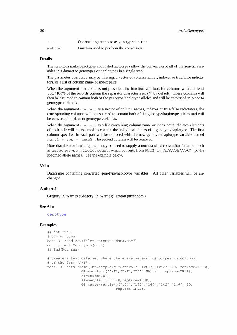
... Optional arguments to as.genotype function
method Function used to perform the conversion.
Details
The functions makeGenotypes and makeHaplotypes allow the conversion of all of the genetic vari-ables in a dataset to genotypes or haplotypes in a single step.
The parameterconvert may be missing, a vector of column names, indexes or true/false indicta-tors, or a list of column name or index pairs.
When the argumentconvert is not provided, the function will look for columns where at leasttol *100% of the records contain the separator charactersep (’/’ by default). These columns willthen be assumed to contain both of the genotype/haplotype alleles and will be converted in-place togenotype variables.
When the argumentconvert is a vector of column names, indexes or true/false indictators, thecorresponding columns will be assumed to contain both of the genotype/haplotype alleles and willbe converted in-place to genotype variables.
When the argumentconvert is a list containing column name or index pairs, the two elementsof each pair will be assumed to contain the individual alleles of a genotype/haplotype. The firstcolumn specified in each pair will be replaced with the new genotype/haplotype variable namedname1 + sep + name2 . The second column will be removed.
Note that themethod argument may be used to supply a non-standard conversion function, suchasas.genotype.allele.count , which converts from [0,1,2] to [’A/A’,’A/B’,’A/C’] (or thespecified allele names). See the example below.
Value
Dataframe containing converted genotype/haplotype variables. All other variables will be un-changed.
Author(s)
Gregory R. Warnes〈[email protected]〉
See Also
genotype
Examples
## Not run:# common casedata <- read.csv(file="genotype_data.csv")data <- makeGenotypes(data)## End(Not run)
# Create a test data set where there are several genotypes in columns# of the form "A/T".test1 <- data.frame(Tmt=sample(c("Control","Trt1","Trt2"),20, replace=TRUE),
G1=sample(c("A/T","T/T","T/A",NA),20, replace=TRUE),N1=rnorm(20),I1=sample(1:100,20,replace=TRUE),G2=paste(sample(c("134","138","140","142","146"),20,
replace=TRUE),

plot.genotype 27
sample(c("134","138","140","142","146"),20,replace=TRUE),
sep=" / "),G3=sample(c("A /T","T /T","T /A"),20, replace=TRUE),comment=sample(c("Possible Bad Data/Lab Error",""),20,
rep=TRUE))
test1
# now automatically convert genotype columnsgeno1 <- makeGenotypes(test1)geno1
# Create a test data set where there are several haplotypes with alleles# in adjacent columns.test2 <- data.frame(Tmt=sample(c("Control","Trt1","Trt2"),20, replace=TRUE),
G1.1=sample(c("A","T",NA),20, replace=TRUE),G1.2=sample(c("A","T",NA),20, replace=TRUE),N1=rnorm(20),I1=sample(1:100,20,replace=TRUE),G2.1=sample(c("134","138","140","142","146"),20,
replace=TRUE),G2.2=sample(c("134","138","140","142","146"),20,
replace=TRUE),G3.1=sample(c("A ","T ","T "),20, replace=TRUE),G3.2=sample(c("A ","T ","T "),20, replace=TRUE),comment=sample(c("Possible Bad Data/Lab Error",""),20,
rep=TRUE))
test2
# specifly the locations of the columns to be paired for haplotypesmakeHaplotypes(test2, convert=list(c("G1.1","G1.2"),6:7,8:9))
# Create a test data set where the data is coded as numeric allele# counts (0-2).test3 <- data.frame(Tmt=sample(c("Control","Trt1","Trt2"),20, replace=TRUE),
G1=sample(c(0:2,NA),20, replace=TRUE),N1=rnorm(20),I1=sample(1:100,20,replace=TRUE),G2=sample(0:2,20, replace=TRUE),comment=sample(c("Possible Bad Data/Lab Error",""),20,
rep=TRUE))
test3
# specifly the locations of the columns, and a non-standard conversionmakeGenotypes(test3, convert=c('G1','G2'), method=as.genotype.allele.count)
plot.genotype Plot genotype object
Description
plot.genotype can plot genotype or allele frequency of a genotype object.

28 power.casectrl
Usage
plot.genotype(x, type=c("genotype", "allele"),what=c("percentage", "number"), ...)
Arguments
x genotype object, as genotype.
type plot "genotype" or "allele" frequency, as character.
what show "percentage" or "number", as character
... Optional arguments forbarplot .
Value
The same as inbarplot .
Author(s)
Gregor GORJANC
See Also
genotype , barplot
Examples
set <- c("A/A", "A/B", "A/B", "B/B", "B/B", "B/B","B/B", "B/C", "C/C", "C/C")
set <- genotype(set, alleles=c("A", "B", "C"), reorder="yes")plot(set)plot(set, type="allele", what="number")
power.casectrl Power for case-control genetics study
Description
Calculate power for case-control genetics study
Usage
power.casectrl(N, gamma = 4.5, p = 0.15, kp = 0.1, alpha = 0.05, fc = 0.5,minh = c("multiplicative", "dominant", "recessive"))
Arguments
N total number of subjects
gamma Relative risk in multiplicative model. Not used in Dominant or Recessive model.
p frequency of A (protective) allele
kp significance level
alpha prevalence of disease
fc fraction of cases
minh mode of inheritance, one of

print.LD 29
Value
power for the specified parameter values.
Author(s)
Michael Man
References
Long, A. D. and C. H. Langley (1997). Genetic analysis of complex traits. Science 275: 1328.
Examples
# single calcpower.casectrl(p=0.1, N=50, gamma=1.1, kp=.1, alpha=5e-2, minh='r')
# for a range of sample sizespower.casectrl(p=0.1, N=c(25,50,100,200,500), gamma=1.1, kp=.1,
alpha=5e-2, minh='r')
# create a power tablefun <- function(p)
power.casectrl(p=p, N=seq(100,1000,by=100), gamma=1.1, kp=.1,alpha=5e-2, minh='recessive')
m <- sapply( X=seq(0.1,0.9, by=0.1), fun )colnames(m) <- seq(0.1,0.9, by=0.1)rownames(m) <- seq(100,1000,by=100)
print(round(m,2))
print.LD Textual and graphical display of linkage disequilibrium (LD) objects
Description
Textual and graphical display of linkage disequilibrium (LD) objects
Usage
print.LD(x, digits = getOption("digits"), ...)print.LD.data.frame(x, ...)
summary.LD.data.frame(object, digits = getOption("digits"),which = c("D", "D'", "r", "X^2", "P-value", "n", " "),rowsep, show.all = FALSE, ...)
print.summary.LD.data.frame(x, digits = getOption("digits"), ...)
plot.LD.data.frame(x,digits=3, colorcut=c(0,0.01, 0.025, 0.5, 0.1, 1),colors=heat.colors(length(colorcut)), textcol="black",marker, which="D'", distance, ...)
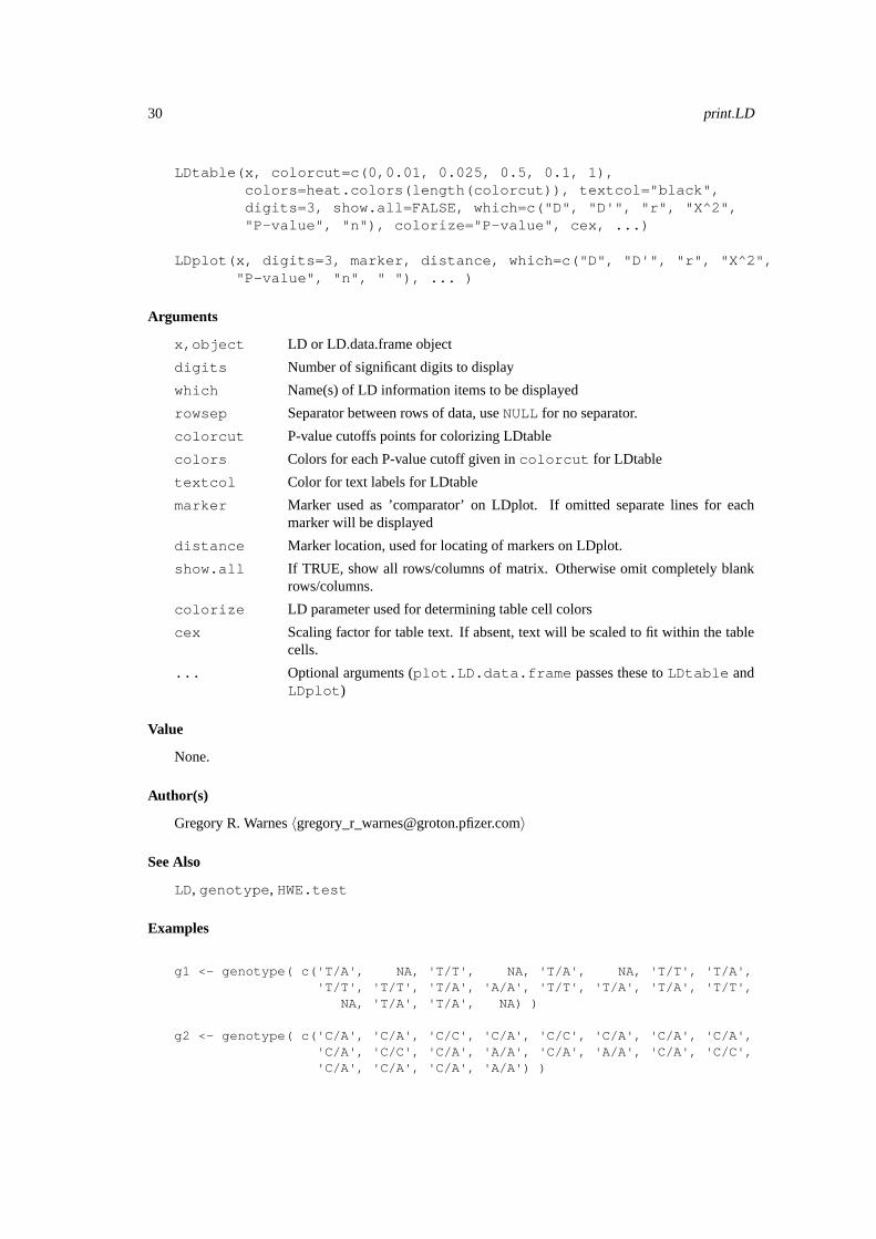
30 print.LD
LDtable(x, colorcut=c(0,0.01, 0.025, 0.5, 0.1, 1),colors=heat.colors(length(colorcut)), textcol="black",digits=3, show.all=FALSE, which=c("D", "D'", "r", "X^2","P-value", "n"), colorize="P-value", cex, ...)
LDplot(x, digits=3, marker, distance, which=c("D", "D'", "r", "X^2","P-value", "n", " "), ... )
Arguments
x,object LD or LD.data.frame object
digits Number of significant digits to display
which Name(s) of LD information items to be displayed
rowsep Separator between rows of data, useNULL for no separator.
colorcut P-value cutoffs points for colorizing LDtable
colors Colors for each P-value cutoff given incolorcut for LDtable
textcol Color for text labels for LDtable
marker Marker used as ’comparator’ on LDplot. If omitted separate lines for eachmarker will be displayed
distance Marker location, used for locating of markers on LDplot.
show.all If TRUE, show all rows/columns of matrix. Otherwise omit completely blankrows/columns.
colorize LD parameter used for determining table cell colors
cex Scaling factor for table text. If absent, text will be scaled to fit within the tablecells.
... Optional arguments (plot.LD.data.frame passes these toLDtable andLDplot )
Value
None.
Author(s)
Gregory R. Warnes〈[email protected]〉
See Also
LD, genotype , HWE.test
Examples
g1 <- genotype( c('T/A', NA, 'T/T', NA, 'T/A', NA, 'T/T', 'T/A','T/T', 'T/T', 'T/A', 'A/A', 'T/T', 'T/A', 'T/A', 'T/T',
NA, 'T/A', 'T/A', NA) )
g2 <- genotype( c('C/A', 'C/A', 'C/C', 'C/A', 'C/C', 'C/A', 'C/A', 'C/A','C/A', 'C/C', 'C/A', 'A/A', 'C/A', 'A/A', 'C/A', 'C/C','C/A', 'C/A', 'C/A', 'A/A') )

summary.genotype 31
g3 <- genotype( c('T/A', 'T/A', 'T/T', 'T/A', 'T/T', 'T/A', 'T/A', 'T/A','T/A', 'T/T', 'T/A', 'T/T', 'T/A', 'T/A', 'T/A', 'T/T','T/A', 'T/A', 'T/A', 'T/T') )
data <- makeGenotypes(data.frame(g1,g2,g3))
# Compute & display LD for one marker pairld <- LD(g1,g2)print(ld)
# Compute LD table for all 3 genotypesldt <- LD(data)
# display the resultsprint(ldt) # textual displayLDtable(ldt) # graphical color-coded tableLDplot(ldt, distance=c(124, 834, 927)) # LD plot vs distance
# more markers makes prettier plots!data <- list()nobs <- 1000ngene <- 20s <- seq(0,1,length=ngene)a1 <- a2 <- matrix("", nrow=nobs, ncol=ngene)for(i in 1:length(s) ){
rallele <- function(p) sample( c("A","T"), 1, p=c(p, 1-p))
if(i==1){
a1[,i] <- sample( c("A","T"), 1000, p=c(0.5,0.5), replace=TRUE)a2[,i] <- sample( c("A","T"), 1000, p=c(0.5,0.5), replace=TRUE)
}else
{p1 <- pmax( pmin( 0.25 + s[i] * as.numeric(a1[,i-1]=="A"),1 ), 0 )p2 <- pmax( pmin( 0.25 + s[i] * as.numeric(a2[,i-1]=="A"),1 ), 0 )a1[,i] <- sapply(p1, rallele )a2[,i] <- sapply(p2, rallele )
}
data[[paste("G",i,sep="")]] <- genotype(a1[,i],a2[,i])}data <- data.frame(data)data <- makeGenotypes(data)
ldt <- LD(data)plot(ldt, digits=2, marker=19) # do LDtable & LDplot on in a single
# graphics window
summary.genotype Allele and Genotype Frequency from a Genotype or Haplotype Object

32 summary.genotype
Description
summary.genotype creates an object containing allele and genotype frequency from agenotypeor haplotype object. print.summary.genotype displays asummary.genotype ob-ject.
Usage
summary.genotype(object, ..., maxsum)print.summary.genotype(x,...,round=2)
Arguments
object, x an object of classgenotype or haplotype (for summary.genotype ) oran object of classsummary.genotype (for print.summary.genotype )
... optional parameters. Ignored bysummary.genotype , passed toprint.matrixby print.summary,genotype .
maxsum specifying any value for the parameter maxsum will causesummary.genotypeto fall back tosummary.factor .
round number of digits to use when displaying proportions.
Details
Specifying any value for the parametermaxsumwill cause fallback tosummary.factor . Thisis so that the functionsummary.dataframe will give reasonable output when it contains agenotype column. (Hopefully we can figure out something better to do in this case.)
Value
The returned value ofsummary.genotype is an object of classsummary.genotype whichis a list with the following components:
locus locus information field (if present) fromx
allele.names vector of allele names
allele.freq A two column matrix with one row for each allele, plus one row forNAvalues (ifpresent). The first column,Count , contains the frequency of the correspondingallele value. The second column,Proportion , contains the fraction of alleleswith the corresponding allele value. Note each observation contains two alleles,thus theCount field sums to twice the number of observations.
genotype.freqA two column matrix with one row for each genotype, plus one row forNAvalues (if present). The first column,Count , contains the frequency of the cor-responding genotype. The second column,Proportion , contains the fractionof genotypes with the corresponding value.
print.summary.genotype silently returns the objectx .
Author(s)
Gregory R. Warnes〈[email protected]〉

undocumented 33
See Also
genotype , HWE.test , allele , homozygote , heterozygote , carrier , allele.countlocus gene marker
Examples
example.data <- c("D/D","D/I","D/D","I/I","D/D","D/D","D/D","D/D","I/I","")
g1 <- genotype(example.data)g1
summary(g1)
undocumented Undocumented functions
Description
These functions are undocumented. Some are internal and not intended for direct use. Some are notyet ready for end users. Others simply haven’t been documented yet.
Usage
Author(s)
Gregory R. Warnes
write.pop.file Create genetics data files
Description
write.pop.file creates a ’pop’ data file, as used by the GenePop (http://wbiomed.curtin.edu.au/genepop/ ) and LinkDos (http://wbiomed.curtin.edu.au/genepop/linkdos.html ) software packages.
write.pedigree.file creates a ’pedigree’ data file, as used by the QTDT software package(http://www.sph.umich.edu/statgen/abecasis/QTDT/ ).
write.marker.file creates a ’marker’ data file, as used by the QTDT software package(http://www.sph.umich.edu/statgen/abecasis/QTDT/ ).
Usage
write.pop.file(data, file = "", digits = 2, description = "Data from R")write.pedigree.file(data, family, pid, father, mother, sex,
file="pedigree.txt")write.marker.file(data, location, file="marker.txt")

34 write.pop.file
Arguments
data Data frame containing genotype objects to be exported
file Output filename
digits Number of digits to use in numbering genotypes, either 2 or 3.
description Description to use as the first line of the ’pop’ file.family, pid, father, mother
Vector of family, individual, father, and mother id’s, respectively.
sex Vector giving the sex of the individual (1=Make, 2=Female)
location Location of the marker relative to the gene of interest, in base pairs.
Details
The format of ’Pop’ files is documented athttp://wbiomed.curtin.edu.au/genepop/help_input.html , the format of ’pedigree’ files is documented athttp://www.sph.umich.edu/csg/abecasis/GOLD/docs/pedigree.html and the format of ’marker’ files is doc-umented athttp://www.sph.umich.edu/csg/abecasis/GOLD/docs/map.html .
Value
No return value.
Author(s)
Gregory R. Warnes〈[email protected]〉
See Also
write.table
Examples
# TBA

Index
∗Topic IOwrite.pop.file , 33
∗Topic designpower.casectrl , 28
∗Topic hplotplot.genotype , 27
∗Topic manipexpectedGenotypes , 14
∗Topic miscci.balance , 10diseq , 11genotype , 15gregorius , 19homozygote , 20HWE.chisq , 1HWE.exact , 3HWE.test , 4LD, 6locus , 22makeGenotypes , 25print.LD , 29summary.genotype , 31undocumented , 33
∗Topic optimizebinsearch , 8
∗Topic programmingbinsearch , 8
==.genotype (genotype ), 15==.haplotype (genotype ), 15[.genotype (genotype ), 15[.haplotype (genotype ), 15[<-.genotype (genotype ), 15[<-.haplotype (genotype ), 15
allele , 2, 17, 32allele (homozygote ), 20allele.count , 17, 32allele.count.2.genotype
(undocumented ), 33allele.count.genotype (genotype ),
15allele.names , 14as.character.gene (locus ), 22as.character.locus (locus ), 22
as.character.marker (locus ), 22as.factor (undocumented ), 33as.factor.allele.genotype
(undocumented ), 33as.factor.default (undocumented ),
33as.factor.genotype
(undocumented ), 33as.genotype (genotype ), 15as.genotype.allele.count
(genotype ), 15as.genotype.character (genotype ),
15as.genotype.default (genotype ), 15as.genotype.factor (genotype ), 15as.genotype.genotype (genotype ),
15as.genotype.haplotype (genotype ),
15as.genotype.table (genotype ), 15as.haplotype (genotype ), 15
barplot , 27binsearch , 8boot , 2, 11, 13bootci , 2, 13bootstrap , 11
carrier , 17, 32carrier (homozygote ), 20chisq.test , 2, 4ci.balance , 10
diseq , 2–5, 11diseq.ci , 2–5, 11
expectedGenotypes , 14
gene , 17, 21, 32gene (locus ), 22gene<- (locus ), 22geno.as.array (undocumented ), 33genotype , 5, 7, 13, 14, 15, 21, 24, 26, 27, 32getgene (locus ), 22getlocus (locus ), 22
35
36 INDEX
getmarker (locus ), 22gregorius , 19
hap (undocumented ), 33hapambig (undocumented ), 33hapenum (undocumented ), 33hapfreq (undocumented ), 33haplotype (genotype ), 15hapmcmc (undocumented ), 33hapshuffle (undocumented ), 33heterozygote , 17, 32heterozygote (homozygote ), 20heterozygote.genotype (genotype ),
15homozygote , 17, 20, 32homozygote.genotype (genotype ), 15htest , 5HWE.chisq , 1, 3, 5HWE.exact , 2, 3, 5HWE.test , 2, 3, 4, 7, 12, 13, 17, 21, 32
is.gene (locus ), 22is.genotype (genotype ), 15is.haplotype (genotype ), 15is.locus (locus ), 22is.marker (locus ), 22
LD, 6LDplot (print.LD ), 29LDtable (print.LD ), 29locus , 17, 21, 22, 32locus<- (locus ), 22
makeGenotypes , 25makeHaplotypes (makeGenotypes ), 25marker , 17, 21, 32marker (locus ), 22marker<- (locus ), 22mknum(undocumented ), 33mourant (undocumented ), 33
nallele (genotype ), 15
optim , 9optimize , 9
plot.genotype , 27plot.LD.data.frame (print.LD ), 29power.casectrl , 28print.allele.count (genotype ), 15print.allele.genotype (genotype ),
15print.diseq (diseq ), 11print.gene (locus ), 22
print.genotype (genotype ), 15print.HWE.test (HWE.test ), 4print.LD , 29print.locus (locus ), 22print.marker (locus ), 22print.summary.genotype
(summary.genotype ), 31print.summary.LD.data.frame
(print.LD ), 29
shortsummary.genotype(undocumented ), 33
summary.genotype , 17, 21, 31summary.LD.data.frame (print.LD ),
29
undocumented , 33uniroot , 9
write.marker.file(write.pop.file ), 33
write.pedigree.file(write.pop.file ), 33
write.pop.file , 33write.table , 34