the generalized minimum spanning tree problem · the generalized minimum spanning tree problem...
TRANSCRIPT

The Generalized Minimum Spanning Tree Problem
Petrica C. Pop
2002
Ph.D. thesisUniversity of Twente
Also available in print:http://www.tup.utwente.nl/catalogue/book/index.jsp?isbn=9036517850
T w e n t e U n i v e r s i t y P r e s s

The Generalized Minimum Spanning Tree Problem

Publisher: Twente University Press,P.O. Box 217, 7500 AE Enschede, the Netherlands, www.tup.utwente.nl
Cover design: Jo Molenaar, [deel4 ontwerpers], EnschedePrint: Océ Facility Services, Enschede
© P.C. Pop, Enschede, 2002No part of this work may be reproduced by print, photocopy or any other meanswithout the permission in writing from the publisher.
ISBN 9036517850

THE GENERALIZED MINIMUM SPANNING TREEPROBLEM
PROEFSCHRIFT
ter verkrijging vande graad van doctor aan de Universiteit Twente,
op gezag van de rector magnificus,prof.dr. F.A. van Vught,
volgens besluit van het College voor Promotiesin het openbaar te verdedigen
op vrijdag 13 december 2002 te 15.00 uur
door
Petrica Claudiu Popgeboren op 30 oktober 1972
te Baia Mare (Roemenië)

Dit proefschrift is goedgekeurd door de promotorprof.dr. U. Faigle
en de assistent-promotorendr. W. Kerndr. G. Still

To the memory of my motherPop Ana


Preface
I want to thank to all the people who helped me, directly and indirectly withthe realization of this thesis.
First of all I want to thank my supervisors prof. U. Faigle and prof. G. Woeg-inger; to prof. U. Faigle also for offering me the opportunity to become aPhD student in the Operations Research group. Besides prof. Faigle and prof.Woeginger there were two persons without whom this work could not be car-ried out in the manner it has been done: Walter Kern and Georg Still. Theiradvice and support during the project were very valuable for me and I enjoyedvery much working with them.
A special word of thanks goes to my daily supervisor Still. The door of hisoffice was always open for me and he has always found time to answer myquestions and to hear my problems.
I am very happy that I met prof. G. Woeginger. I am grateful to him for theuseful discussions we had and his comments regarding my research.
I want to express my gratitude to prof. C. Hoede, prof. R. Dekker, prof. A.van Harten and prof. M. Labbe for participating in the promotion committeeand for their interest in my research.
A word of thanks goes to my colleagues from the Department of DiscreteMathematics, Operations Research and Stochastic and in particular to my for-mer office-mates: Cindy Kuipers and Daniele Paulusma who offered me apleasant working environment.
During the time spent in Twente I made many good friends and I am surethat without them my life in the Netherlands would not be so comfortable.Special thanks to Octav, Rita, Natasa, Goran, Adriana, Marisela, Valentinaand Andrei.
At last but not at least I want to thank to my family.
vii

In particular I am most grateful to my wife, my parents and my brother. Iwould not have been where I am now without their unconditioned love andsupport.
Baia Mare, 10 November 2002
Petrica C. Pop
viii

Contents
1 Introduction 11.1 Combinatorial and Integer Optimization . . . . . . . . . . . . 2
1.1.1 Complexity theory . . . . . . . . . . . . . . . . . . . 31.1.2 Heuristic and Relaxation Methods . . . . . . . . . . . 61.1.3 Dynamic programming . . . . . . . . . . . . . . . . . 7
1.2 Polyhedral theory . . . . . . . . . . . . . . . . . . . . . . . . 81.3 Graph theory . . . . . . . . . . . . . . . . . . . . . . . . . . 101.4 Outline of the thesis . . . . . . . . . . . . . . . . . . . . . . . 13
2 The Generalized Minimum Spanning Tree Problem 152.1 Generalized Combinatorial Optimization
Problems . . . . . . . . . . . . . . . . . . . . . . . . . . . . 162.2 Minimum Spanning Trees . . . . . . . . . . . . . . . . . . . 172.3 Definition of the GMST problem . . . . . . . . . . . . . . . . 192.4 The GMST problem on trees . . . . . . . . . . . . . . . . . . 212.5 Complexity of the GMST problem . . . . . . . . . . . . . . . 232.6 Polynomially solvable cases of the GMST
problem . . . . . . . . . . . . . . . . . . . . . . . . . . . . . 232.7 Applications of the GMST problem . . . . . . . . . . . . . . 252.8 A variant of the GMST problem . . . . . . . . . . . . . . . . 26
3 Polyhedral aspects of the GMST Problem 293.1 Introduction . . . . . . . . . . . . . . . . . . . . . . . . . . . 303.2 Formulations for the undirected problem . . . . . . . . . . . . 313.3 Formulations for the directed problem . . . . . . . . . . . . . 353.4 Flow based formulations . . . . . . . . . . . . . . . . . . . . 383.5 Local-global formulation of the GMST problem . . . . . . . . 41
3.5.1 Local solution using dynamic programming . . . . . . 42
ix

3.5.2 Local solution using integer linear programming . . . 433.5.3 Local-global formulation of the GMST problem . . . . 45
3.6 Solution procedure and computational results . . . . . . . . . 463.7 Concluding remarks . . . . . . . . . . . . . . . . . . . . . . . 52
4 Approximation Algorithms 554.1 Introduction . . . . . . . . . . . . . . . . . . . . . . . . . . . 564.2 Positive Results: the Design of the Approximation Algorithms 584.3 A negative result for the GMST problem . . . . . . . . . . . . 604.4 An Approximation Algorithm for Bounded Cluster Size . . . . 63
4.4.1 An integer programming formulation of the GMSTproblem . . . . . . . . . . . . . . . . . . . . . . . . . 64
4.4.2 An Approximation Algorithm for the GMST problem . 644.4.3 Auxiliary results . . . . . . . . . . . . . . . . . . . . 654.4.4 Performance Bounds . . . . . . . . . . . . . . . . . . 68
4.5 Concluding remarks . . . . . . . . . . . . . . . . . . . . . . . 71
5 Linear Programming, Lagrangian and Semidefinite Relaxations 735.1 Lagrangian Relaxation . . . . . . . . . . . . . . . . . . . . . 75
5.1.1 Basic principles . . . . . . . . . . . . . . . . . . . . . 755.1.2 Solving the Lagrangian dual . . . . . . . . . . . . . . 78
5.2 Semidefinite Programming . . . . . . . . . . . . . . . . . . . 805.2.1 Geometry . . . . . . . . . . . . . . . . . . . . . . . . 815.2.2 Duality and Optimality Conditions . . . . . . . . . . . 81
5.3 Lagrangian duality for quadratic programs . . . . . . . . . . . 855.3.1 Dualizing a quadratic problem . . . . . . . . . . . . . 855.3.2 The lifting procedure . . . . . . . . . . . . . . . . . . 88
5.4 Application to 0-1 programming . . . . . . . . . . . . . . . . 895.4.1 Linear dualization . . . . . . . . . . . . . . . . . . . 895.4.2 Complete dualization . . . . . . . . . . . . . . . . . 905.4.3 Boolean dualization . . . . . . . . . . . . . . . . . . 915.4.4 Inequality constraints . . . . . . . . . . . . . . . . . . 93
5.5 Concluding remarks . . . . . . . . . . . . . . . . . . . . . . . 94
6 Solving the GMST problem with Lagrangian Relaxation 956.1 A strong formulation of the GMST problem . . . . . . . . . . 966.2 Defining a Lagrangian problem . . . . . . . . . . . . . . . . . 976.3 The Subgradient Procedure . . . . . . . . . . . . . . . . . . . 98
x

6.4 Computational Results . . . . . . . . . . . . . . . . . . . . . 1016.5 Concluding remarks . . . . . . . . . . . . . . . . . . . . . . . 106
7 Heuristic Algorithms 1077.1 Introduction . . . . . . . . . . . . . . . . . . . . . . . . . . . 1087.2 Local and global optima . . . . . . . . . . . . . . . . . . . . 1087.3 Local Search . . . . . . . . . . . . . . . . . . . . . . . . . . 1097.4 Simulated Annealing . . . . . . . . . . . . . . . . . . . . . . 112
7.4.1 Introduction . . . . . . . . . . . . . . . . . . . . . . . 1127.4.2 The annealing algorithm . . . . . . . . . . . . . . . . 113
7.5 Solving the GMST problem with Simulated Annealing . . . . 1157.5.1 The local-global formulation of the GMST problem . . 1157.5.2 Generic decisions . . . . . . . . . . . . . . . . . . . . 1167.5.3 Problem specific decisions . . . . . . . . . . . . . . . 1187.5.4 A computational example . . . . . . . . . . . . . . . 120
Bibliography 123
Subject Index 129
Summary 133
xi


Chapter 1
Introduction
In this thesis we use several combinatorial optimization techniques to solvethe Generalized Minimum Spanning Tree problem. For an overview of gen-eral combinatorial optimization techniques, we refer to the books of Nemhauserand Wolsey [55], Papadimitriou and Steiglitz [57] and Schrijver [69].
In this chapter we present fundamental concepts of Combinatorial and Integeroptimization (Section 1.1), Polyhedral theory (Section 1.2) and Graph theory(Section 1.3). We end the chapter with an outline of the thesis.
1
1.1 Combinatorial and Integer Optimization
Combinatorial Optimization is the process of finding one or more best (op-timal) solutions in a well defined discrete problem space, i.e. a space con-taining a finite set of possible solutions, that optimizes a certain function, theso-calledobjective function. The finite set of possible solutions can be de-scribed by inequality and equality constraints, and by integrality constraints.The integrality constraints force the variables to be integers. The set of pointsthat satisfy all these constraints is called the(feasible) solution set.
Such problems occur in almost all fields of management (e.g. finance, mar-keting, production, scheduling, inventory control, facility location, etc.), aswell as in many engineering disciplines (e.g. optimal design of waterwaysor bridges, design and analysis of data networks, energy resource-planningmodels, logistic of electrical power generation and transport, etc). A surveyof applications of combinatorial optimization is given by Grotschel in [30].
Combinatorial Optimization models are often referred to as integer program-ming models where some or all of the variables can take on only a finitenumber of alternative possibilities.
In this thesis we consider combinatorial optimization problems for which theobjective function and the constraints are linear and the variables are integers.These problems are calledinteger programming problems:
min cT x(IP ) s.t. Ax ≤ b
x ∈ Zn
whereZn is the set of integraln-dimensional vectors,x = (x1, ..., xn) is anintegern-vector andc is an integern-vector. Furthermore, we letm denotethe number of inequality contraints,A an m× n matrix andb an m-vector.If we allow some variablesxi to be continous instead of integer, i.e.xi ∈ Rinstead ofxi ∈ Z, then we obtain amixed integer programming problem, de-noted by (MIP). For convenience, we discuss integer linear programs that areminimizationproblems withbinary variables, i.e. the integer variables arerestricted to values 0 or 1. In Chapter 3 we present several integer program-ming and mixed integer programming models of the Generalized MinimumSpanning Tree problem.
2

Solving integer programming problems can be a difficult task. The difficultyarises from the fact that unlike linear programming, where the feasible regionis a convex set, in integer problems one must search a lattice of feasible pointsor, in the mixed integer case a set of disjoint halflines or line segments to findan optimal solution. Therefore, unlike linear programming where, due tothe convexity of the problem, we can exploit the fact that any local solutionis a global optimum, integer programming problems may have many ”localoptima” and finding a global optimum to the problem requires one to provethat a particular solution dominates all feasible points by arguments other thanthe calculus-based derivative approaches of convex programming.
When optimizing combinatorial problems, there is always a trade-off betweenthe computational effort (and hence the running time) and the quality of theobtained solution. We may either try to solve the problem to optimality withan exact algorithm, or choose for anapproximationor heuristic algorithm,which uses less running time but does not guarantee optimality of the solution.
1.1.1 Complexity theory
The first step in studying a combinatorial problem is to find out whether theproblem is ”easy” or ”hard”. Complexity theory deals with this kind of prob-lem classification. In this subsection we summarize the most important con-cepts of complexity theory. Most approaches are taken from the books men-tioned before and from the book of Grotschel, Lovasz and Schrijver [31].
An algorithm is a list of instructions that solves everyinstanceof a problemin a finite number of steps. (This means also: the algorithm detects that theproblem instance has no solution).
The sizeof a problem is the amount of information needed to represent theinstance. The instance is assumed to be described (encoded) by a string ofsymbols. Therefore, the size of an instance equals the number of symbols inthe string.
The running timeof a combinatorial optimization algorithm is measured byan upper bound on the number of elementary arithmetic operations (adding,subtracting, multiplying, dividing and comparing numbers) it needs for anyvalid input, expressed as a function of the input size. Theinput is the dataused to represent a problem instance. If the input size is measured bys,then the running time of the algorithm is expressed asO(f(s)), if there are
3

constantsb ands0 such that the number of steps for any instance withs ≥ s0
is bounded from above bybf(s). We say that the running time of such analgorithm is of orderf(s).
An algorithm is said to be apolynomial time algorithmwhen its running timeis bounded by a polynomial function,f(s). An algorithm is said to be anex-ponential time algorithmwhen its running time is bounded by an exponentialfunction (e.g.O(2p(s))).
The theory of complexity concerns in the first place decision problems. Ade-cision problemis a question that can be answered only by ”yes” or ”no”. Forexample in the case of the integer programming problem (IP ) the decisionproblem is:
Given an instance of (IP ) and an integerL is there a feasiblesolutionx such thatcT x ≤ L?
For a combinatorial optimization problem we have the following: if one cansolve the decision problem efficiently, then one can solve the correspondingopimization problem efficiently.
Decision problems that are solvable in polynomial time are considered to be”easy” , the class of these problems is denoted byP. P includes for examplelinear programming and the minimum spanning tree problem.
The class of decision problems solvable in exponential time is denoted byEXP . Most combinatorial optimization problems belong to this class. If aproblem is inEXP \ P, then solving large instances of this problem will bedifficult. To distinguish between ”easy” and ”hard” problems we first describea class of problems that containsP.
The complexity classNP is defined as the class of decision problems that aresolvable by a so-callednon-deterministic algorithm. A decision problem issaid to be inNP if for any input that has a positive answer, there is a certifi-cate from which the correctness of this answer can be derived in polynomialtime.
Obviously,P ⊆ NP holds. It is widely assumed thatP = NP is very un-likely. The classNP contains a subclass of problems that are considered tobe the hardest problems inNP. These problems are calledNP-completeproblems. Before giving the definition of anNP-completedecision prob-lem we explain the technique of polynomially transforming one problem intoanother. LetΠ1 andΠ2 be two decision problems.
4

Definition 1.1 A polynomial transformation is an algorithmA that, for ev-ery instanceσ1 of Π1 produces in polynomial time an instanceσ2 of Π2 suchthat the following holds: for every instanceσ1 ofΠ1, the answer toσ1 is ”yes”if and only if the answer to instanceσ2 of Π2 is ”yes”. ¤
Definition 1.2 A decision problemΠ is calledNP-complete ifΠ is in NPand every otherNP decision problem can be polynomially transformed intoΠ. ¤
Clearly, if anNP-completeproblem can be solved in polynomial time, thenall problems inNP can be solved in polynomial time, henceP = NP. Thisexplains why theNP-completeproblems are considered to be the hardestproblems inNP. Note that polynomially transformability is a transitive re-lation, i.e if Π1 is polynomially transformable toΠ2 andΠ2 is polynomiallytransformable toΠ3, thenΠ1 is polynomially transformable toΠ3. Therefore,if we want to prove that a decision problemΠ isNP-complete, then we onlyhave to show that
(i) Π is inNP.
(ii) Some decision problem already known to beNP-completecan be poly-nomially transformed toΠ.
Now we want to focus on combinatorial optimization problems. Thereforewe extend the concept of polynomially transformability. LetΠ1 andΠ2 betwo problems (not necessarily decision problems).
Definition 1.3 A polynomial reduction from Π1 to Π2 is an algorithmA1
that, solvesΠ1 by using an algorithmA2 for Π2 as a subroutine such that, ifA2 were a polynomial time algorithm forΠ2, thenA1 would be a polynomialtime algorithm forΠ1. ¤
Definition 1.4 An optimization problemΠ is calledNP-hard if there existsanNP-complete decision problem that can be polynomially reduced toΠ. ¤
Cearly, an optimization problem isNP-hard if the corresponding decisionproblem isNP-complete. In particular, the Generalized Minimum SpanningTree problem isNP-hard (see Section 2.5).
5

1.1.2 Heuristic and Relaxation Methods
As we have seen, once established that a combinatorial problem isNP-hard,it is unlikely that it can be solved by a polynomial algorithm.
Finding good solutions for hard minimization problems in combinatorial op-timization requires the consideration of two issues:
• calculation of an upper bound that is as close as possible to the opti-mum;
• calculation of a lower bound that is as close as possible to the optimum.
General techniques for generating good upper bounds are essentially heuristicmethods such as Simulated Annealing, Tabu Search, Genetic Algorithms, etc.,which we are going to consider in chapter 7 of the thesis. In addition, for anyparticular problem, we may well have techniques which are specific to theproblem being solved.
On the question of lower bounds, we present in Chapter 5 the following tech-niques:
• Linear Programming (LP) relaxationIn LP relaxation we take an integer (or mixed-integer) programmingformulation of the problem and relax the integrality requirement on thevariables. This gives a linear program which can either be solved ex-actly using a standard algorithm (simplex or interior point); or heuristi-cally (dual ascent). The solution value obtained for this linear programgives a lower bound on the optimal solution to the original minimizationproblem.
• Lagrangian relaxationThe general idea of Lagrangian relaxation is to ”relax” (dualize) some(or all) constraints by adding them to the objective function using La-grangian multipliers. Choosing ”good” values for the Lagrangian mul-tipliers is of key importance in terms of quality of the lower boundgenerated.
• Semidefinite programming (SDP) relaxationCombinatorial optimization problems often involve binary (0,1 or +1,-1) decision variables. These can be modelled using quadratic con-straintsx2−x = 0, andx2 = 1, respectively. Using the positive semidef-inite matrixX = xxT , we can lift the problem into a matrix space and
6
obtain a Semidefinite Programming Relaxation by ignoring the rank onerestriction on X, see e.g. [49]. These semidefinite relaxations providetight bounds for many classes of hard problems and in addition can besolved efficiently by interior-point methods.
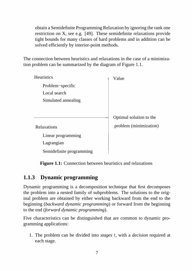
The connection between heuristics and relaxations in the case of a minimiza-tion problem can be summarized by the diagram of Figure 1.1.
Value
Optimal solution to the
problem (minimization)
Heuristics
Problem−specific
Semidefinite programming
Local search
Simulated annealing
Relaxations
Linear programming
Lagrangian
Figure 1.1: Connection between heuristics and relaxations
1.1.3 Dynamic programming
Dynamic programming is a decomposition technique that first decomposesthe problem into a nested family of subproblems. The solutions to the orig-inal problem are obtained by either working backward from the end to thebeginning (backward dynamic programming) or forward from the beginningto the end (forward dynamic programming).
Five characteristics can be distinguished that are common to dynamic pro-gramming applications:
1. The problem can be divided intostagest, with a decisionrequired ateach stage.
7
2. Each staget has a set ofstates{it} associated with it. At any stage, astate holds all the information that is needed to make a decision.
3. The decision chosen at any stage determines how the state at the cur-rent stage is transformed into the state at the next stage, as well as theimmediately earned reward or cost.
4. Given the current state, the optimal decision for each remaining stagesmust not depend on previously reached states or previously chosen de-cisions. This is the so-calledprinciple of optimalityfor dynamic pro-gramming (Bellman, [3]).
5. If the states for the problem have been classified into one ofT stages,there must be arecursionthat relates the cost or reward earned duringstagest, t + 1, ..., T to the cost or reward earned from stagest + 1, t +2, ..., T .
Dynamic programming algorithms are computationally efficient, as long asthe state space does not become too large. However, when the state space be-comes too large implementation problems may occur (e.g. insufficient com-puter memory), or excessive computational time may be required to use dy-namic programming to solve the problem. For more information about dy-namic programming we refer to Bellman [3] and Dreyfus and Law [12].
1.2 Polyhedral theory
The theory we discuss in this section is derived from the the books of Schrijver[69] and Grotschel, Lovasz and Schrijver [31].
Consider a set of pointsX = {x1, . . . , xk} ⊆ Rn and a vectorλ ∈ Rk. Thelinear combinationx =
∑ki=1 λix
i is anaffine combinationif∑k
i=1 λi = 1,andx is called aconvex combinationif in addition to
∑ki=1 λi = 1 we have
λi ≥ 0. X is calledlinearly (affinely) independentif no point xi ∈ X can bewritten as a linear (affine) combination of the other points inX.
A subsetS ⊆ Rn is convexif for every finite number of pointsx1, . . . , xk ∈ Sany convex combination of these points is a member ofS.
A nonempty setC ⊆Rn is called aconvex coneif λx+µy ∈C for all x, y ∈Cand for all real numbersλ,µ ≥ 0.
8

A convex setP ⊆ Rn is apolyhedronif there exists anm× n matrixA and avectorb ∈ Rm such that
P = P (A, b) = {x ∈ Rn | Ax ≤ b}.We callAx ≤ b asystem of linear inequalities.
A polyhedronP ⊆ Rn is boundedif there exist vectorsl, u ∈ Rn such thatl ≤ x ≤ u for all x ∈ P . A bounded polyhedron is called apolytope.
For our purposes, only rational polyhedra are of interest. A polyhedron isrational if it is the solution set of a systemAx≤ b of linear inequalities, whereA andb are rational. From now on we will implicitly assume a polyhedron tobe rational.
A point x ∈ P is called avertexof P if x cannot be written as a convexcombination of other points inP .
Thedimensionof a polyhedronP ⊆ Rn is equal to the maximum number ofaffinely independent points inP minus1. An implicit equalityof the systemAx≤ b is an inequality
∑nj=1 aijxj ≤ bi of that system such that
∑nj=1 aijxj =
bi for all vectorsx ∈ P (A, b). For Ax ≤ b we denote the (sub)system ofimplicit equalities byA=x ≤ b=. Let rank(A) denote therank of a matrix,i.e., the maximum number of linearly independent row vectors. We have thefollowing standard result.
Theorem 1.1 The dimension of a polyhedronP (A, b) ⊆ Rn is equal ton−rank(A=). ¤
A subsetH ⊆ Rn is called ahyperplaneif there exists a vectorh ∈ Rn and anumberα ∈ R such that
H = {x ∈ Rn | hT x = α}.
A separating hyperplanefor a convex setS and vectory /∈ S is a hyperplanegiven by a vectorh ∈Rn and a numberα ∈R such thathT x≤ α andhT y > αholds for allx ∈ S.
Theseparation problemfor a polyhedronP ⊆ Rn is, given a vectorx ∈ Rn,to decide whetherx ∈ P or not, and, ifx /∈ P , to find a separating hyperplanefor P andx. A separation algorithmfor a polyhedronP is an algorithm thatsolves the separation problem forP .
9
Linear programming(LP) deals with maximizing or minimizing a linear func-tion over a polyhedron. IfP ⊆ Rn is a polyhedron andd ∈ Rn, then we callthe optimization problem
(LP ) max{dT x | x ∈ P}a linear program. A vectorx ∈ P is called afeasible solutionof the linearprogram andx∗ is called anoptimal solutionif x∗ is feasible anddT x∗ ≥ dT xfor all feasible solutionsx. We say that (LP ) is unboundedif for all λ ∈ Rthere exists a feasible solutionx∗ ∈ P such thatdT x∗ ≥ λ, If (LP ) has nooptimal solution then it is either infeasible or unbounded.
The first polynomial time algorithm for LP is the so-calledellipsoid algo-rithm, proposed by Khachiyan [43]. Although of polynomial running time,the algorithm is impractical for LP. Nevertheless, it has extensive theoreticalapplications in combinatorial optimization: the stable set problem on perfectgraphs for example can be solved in polynomial time using the ellipsoid al-gorithm. Grotschel, Lovasz and Schrijver [32] refined this method in such away that the computational complexity of optimizing a linear function over aconvex setS depends on the complexity of the separation problem forS. In1984, Karmarkar [42] presented another polynomial time algorithm for LP.His algorithm avoids the combinatorial complexity (inherent in the simplexalgorithm) of the vertices, edges and faces of the polyhedron by staying insidethe polyhedron. His algorithm lead to many other algorithms for LP based onsimilar ideas. These algorithms are known asinterior point methods.
1.3 Graph theory
In this section we include some terminology for readers not familiar withgraph theory. For more details on graph theory we refer to the book of Bondyand Murty [7].
A graphG is an ordered pair(V,E), whereV is a nonempty, finite set calledthenode setandE is a set of (unordered) pairs (i, j) with i, j ∈ V called theedge set.
The elements ofV are callednodesand the elements ofE are callededges.If e = (i, j) ∈ E we say that nodei and nodej areadjacent. In such a casei andj are called theend pointsof e or incidentwith e. Furthermore, we say
10
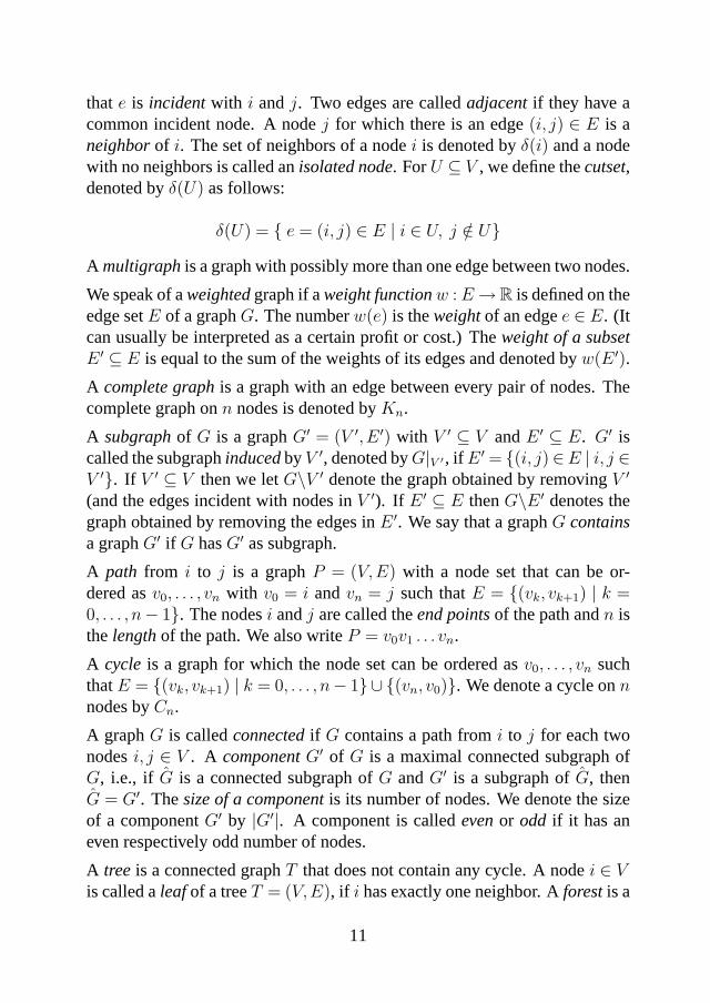
thate is incidentwith i andj. Two edges are calledadjacentif they have acommon incident node. A nodej for which there is an edge(i, j) ∈ E is aneighborof i. The set of neighbors of a nodei is denoted byδ(i) and a nodewith no neighbors is called anisolated node. ForU ⊆ V , we define thecutset,denoted byδ(U) as follows:
δ(U) = { e = (i, j) ∈ E | i ∈ U, j /∈ U}A multigraphis a graph with possibly more than one edge between two nodes.
We speak of aweightedgraph if aweight functionw : E →R is defined on theedge setE of a graphG. The numberw(e) is theweightof an edgee ∈ E. (Itcan usually be interpreted as a certain profit or cost.) Theweight of a subsetE ′ ⊆ E is equal to the sum of the weights of its edges and denoted byw(E ′).
A complete graphis a graph with an edge between every pair of nodes. Thecomplete graph onn nodes is denoted byKn.
A subgraphof G is a graphG′ = (V ′,E ′) with V ′ ⊆ V andE ′ ⊆ E. G′ iscalled the subgraphinducedbyV ′, denoted byG|V ′, if E ′ = {(i, j)∈E | i, j ∈V ′}. If V ′ ⊆ V then we letG\V ′ denote the graph obtained by removingV ′
(and the edges incident with nodes inV ′). If E ′ ⊆ E thenG\E ′ denotes thegraph obtained by removing the edges inE ′. We say that a graphG containsa graphG′ if G hasG′ as subgraph.
A path from i to j is a graphP = (V,E) with a node set that can be or-dered asv0, . . . , vn with v0 = i andvn = j such thatE = {(vk, vk+1) | k =0, . . . , n− 1}. The nodesi andj are called theend pointsof the path andn isthe lengthof the path. We also writeP = v0v1 . . . vn.
A cycle is a graph for which the node set can be ordered asv0, . . . , vn suchthatE = {(vk, vk+1) | k = 0, . . . , n− 1} ∪ {(vn, v0)}. We denote a cycle onnnodes byCn.
A graphG is calledconnectedif G contains a path fromi to j for each twonodesi, j ∈ V . A componentG′ of G is a maximal connected subgraph ofG, i.e., if G is a connected subgraph ofG andG′ is a subgraph ofG, thenG = G′. Thesize of a componentis its number of nodes. We denote the sizeof a componentG′ by |G′|. A component is calledevenor odd if it has aneven respectively odd number of nodes.
A tree is a connected graphT that does not contain any cycle. A nodei ∈ Vis called aleafof a treeT = (V,E), if i has exactly one neighbor. Aforestis a
11

graph (not necessarily connected) that does not contain any cycle. Aspanningtreeof G = (V,E) is a tree(V ′,E ′) with V ′ = V .
A node coverin a graphG = (V,E) is a subsetV ′ of V such that every edgein E is incident with a node inV ′.
If the pairs(i, j) in the edge set of a graph are ordered, then we speak ofa directed graphor digraph and we call such an ordered pair(i, j) an arc.In this case the edge set is usually denoted byA. The arca = (i, j) ∈ A isan outcoming arcof nodei and is anincoming arcof nodej. The set ofoutcoming arcs of a nodei is denoted byδ+(i) and the set of incoming arcsof a nodei is denoted byδ−(i). To this end, call a subsetA
′of A ans− t cut
if A′= δ+(U) for some subsetU of V satisfyings ∈ U andt /∈ U , where for
everyU ⊆ V , δ+(U) is defined as follows:
δ+(U) = { (i, j) ∈ A | i ∈ U, j /∈ U}
Let D = (V,A) be a directed graph and letr, s ∈ V . A functionf : A→ R iscalled anr− s flow if
(i) f(a) ≥ 0 for eacha ∈ A,
(ii)∑
a∈δ+(v)
f(a) =∑
a∈δ−(v)
f(a) for eachv ∈ V \ {r, s}.
The value of anr− s flow f is, by definition:
value(f) :=∑
a∈δ+(r)
f(a)−∑
a∈δ−(r)
f(a).
So the value is the net amount of flow leavingr. It is also equal to the netamount of flow enterings.
Let c : A→ R+, be acapacity function. We say that a flowf is underc if
f(a) ≤ c(a) for eacha ∈ A.
Themaximum flow problemnow is to find anr− s flow underc, of maximumvalue. To formulate the so-called min-max relation, we define thecapacityofa cutδ+(U) by
12
c(δ+(U)) :=∑
a∈δ+(U)
c(a).
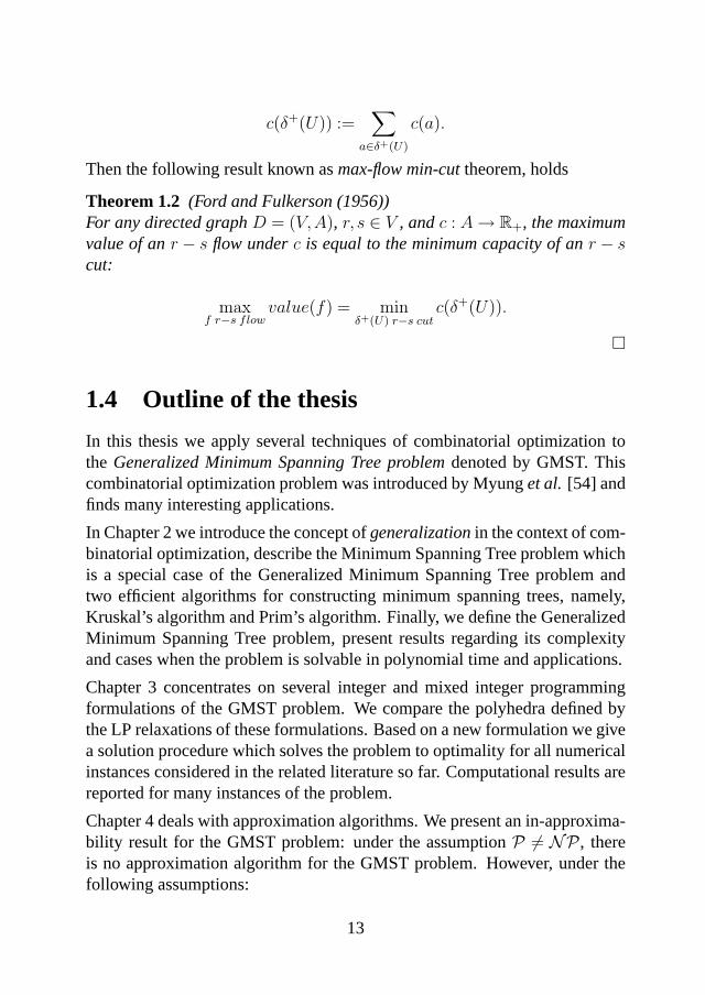
Then the following result known asmax-flow min-cuttheorem, holds
Theorem 1.2 (Ford and Fulkerson (1956))For any directed graphD = (V,A), r, s ∈ V , andc : A→ R+, the maximumvalue of anr − s flow underc is equal to the minimum capacity of anr − scut:
maxf r−s flow
value(f) = minδ+(U) r−s cut
c(δ+(U)).
¤
1.4 Outline of the thesis
In this thesis we apply several techniques of combinatorial optimization tothe Generalized Minimum Spanning Tree problemdenoted by GMST. Thiscombinatorial optimization problem was introduced by Myunget al. [54] andfinds many interesting applications.
In Chapter 2 we introduce the concept ofgeneralizationin the context of com-binatorial optimization, describe the Minimum Spanning Tree problem whichis a special case of the Generalized Minimum Spanning Tree problem andtwo efficient algorithms for constructing minimum spanning trees, namely,Kruskal’s algorithm and Prim’s algorithm. Finally, we define the GeneralizedMinimum Spanning Tree problem, present results regarding its complexityand cases when the problem is solvable in polynomial time and applications.
Chapter 3 concentrates on several integer and mixed integer programmingformulations of the GMST problem. We compare the polyhedra defined bythe LP relaxations of these formulations. Based on a new formulation we givea solution procedure which solves the problem to optimality for all numericalinstances considered in the related literature so far. Computational results arereported for many instances of the problem.
Chapter 4 deals with approximation algorithms. We present an in-approxima-bility result for the GMST problem: under the assumptionP 6= NP, thereis no approximation algorithm for the GMST problem. However, under thefollowing assumptions:
13

• the graph has bounded cluster size,
• the cost function is strictly positive and satisfies the triangle inequality,i.e. cij + cjk ≥ cik for all i, j, k ∈ V ,
we present a polynomial approximation algorithm for the GMST problem.
In Chapter 5 we discuss the basic theory of Lagrangian and semidefinite pro-gramming relaxations and we study different possible dualizations for a gen-eral 0-1 program.
In Chapter 6 we present an algorithm based on Lagrangian relaxation of abidirectional multicommodity flow formulation of the GMST problem. Thesubgradient optimization algorithm is used to obtain lower bounds. Compu-tational results are reported for many instances of the problem.
Chapter 7 deals with heuristic algorithms. We present the basic theory of localsearch and other concepts underlying many modern heuristic techniques, suchas Simulated Annealing, Tabu Search Genetic Algorithms, etc., and we solvethe GMST problem with Simulated Annealing. Computational results arereported.
14

Chapter 2
The Generalized MinimumSpanning Tree Problem
The aim of this chapter is to introduce the Generalized Minimum SpanningTree problem. In the first section we discuss the concept ofgeneralizationand provide a list of problems defined on graphs that have ageneralizedstruc-ture. In the second section we describe the Minimum Spanning Tree problemwhich is a special case of the Generalized Minimum Spanning Tree prob-lem and two efficient algorithms for constructing minimum spanning trees,namely, Kruskal’s algorithm and Prim’s algorithm. The next sections focuson the GMST problem: we give the definition of the problem, present resultsregarding its complexity and cases when the problem is solvable in polyno-mial time and applications. As well as in the last section we present a variantof the GMST problem.
15
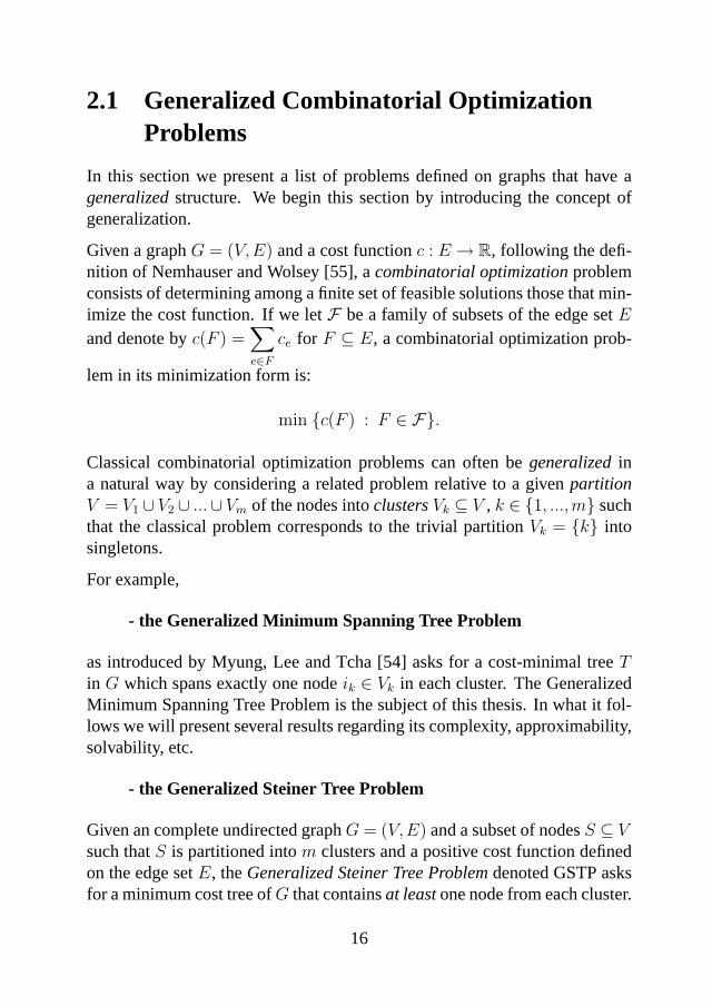
2.1 Generalized Combinatorial OptimizationProblems
In this section we present a list of problems defined on graphs that have ageneralizedstructure. We begin this section by introducing the concept ofgeneralization.
Given a graphG = (V,E) and a cost functionc : E → R, following the defi-nition of Nemhauser and Wolsey [55], acombinatorial optimizationproblemconsists of determining among a finite set of feasible solutions those that min-imize the cost function. If we letF be a family of subsets of the edge setE
and denote byc(F ) =∑e∈F
ce for F ⊆ E, a combinatorial optimization prob-
lem in its minimization form is:
min {c(F ) : F ∈ F}.
Classical combinatorial optimization problems can often begeneralizedina natural way by considering a related problem relative to a givenpartitionV = V1 ∪ V2 ∪ ...∪ Vm of the nodes intoclustersVk ⊆ V , k ∈ {1, ...,m} suchthat the classical problem corresponds to the trivial partitionVk = {k} intosingletons.
For example,
- the Generalized Minimum Spanning Tree Problem
as introduced by Myung, Lee and Tcha [54] asks for a cost-minimal treeTin G which spans exactly one nodeik ∈ Vk in each cluster. The GeneralizedMinimum Spanning Tree Problem is the subject of this thesis. In what it fol-lows we will present several results regarding its complexity, approximability,solvability, etc.
- the Generalized Steiner Tree Problem
Given an complete undirected graphG = (V,E) and a subset of nodesS ⊆ Vsuch thatS is partitioned intom clusters and a positive cost function definedon the edge setE, theGeneralized Steiner Tree Problemdenoted GSTP asksfor a minimum cost tree ofG that containsat leastone node from each cluster.
16
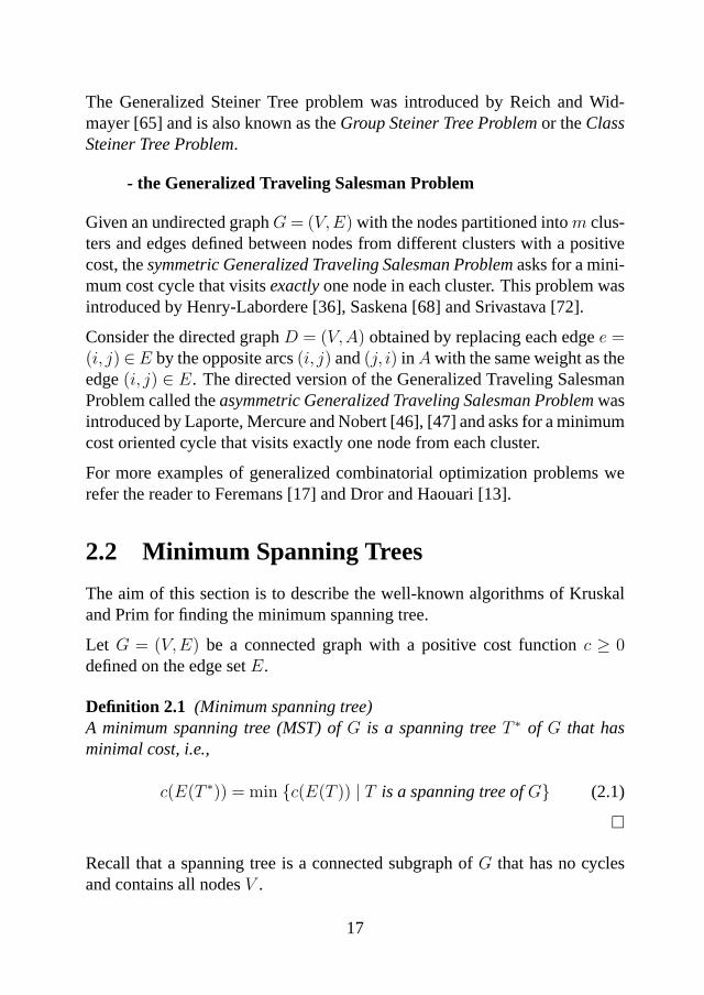
The Generalized Steiner Tree problem was introduced by Reich and Wid-mayer [65] and is also known as theGroup Steiner Tree Problemor theClassSteiner Tree Problem.
- the Generalized Traveling Salesman Problem
Given an undirected graphG = (V,E) with the nodes partitioned intom clus-ters and edges defined between nodes from different clusters with a positivecost, thesymmetric Generalized Traveling Salesman Problemasks for a mini-mum cost cycle that visitsexactlyone node in each cluster. This problem wasintroduced by Henry-Labordere [36], Saskena [68] and Srivastava [72].
Consider the directed graphD = (V,A) obtained by replacing each edgee =(i, j) ∈E by the opposite arcs(i, j) and(j, i) in A with the same weight as theedge(i, j) ∈ E. The directed version of the Generalized Traveling SalesmanProblem called theasymmetric Generalized Traveling Salesman Problemwasintroduced by Laporte, Mercure and Nobert [46], [47] and asks for a minimumcost oriented cycle that visits exactly one node from each cluster.
For more examples of generalized combinatorial optimization problems werefer the reader to Feremans [17] and Dror and Haouari [13].
2.2 Minimum Spanning Trees
The aim of this section is to describe the well-known algorithms of Kruskaland Prim for finding the minimum spanning tree.
Let G = (V,E) be a connected graph with a positive cost functionc ≥ 0defined on the edge setE.
Definition 2.1 (Minimum spanning tree)A minimum spanning tree (MST) ofG is a spanning treeT ∗ of G that hasminimal cost, i.e.,
c(E(T ∗)) = min {c(E(T )) | T is a spanning tree ofG} (2.1)
¤
Recall that a spanning tree is a connected subgraph ofG that has no cyclesand contains all nodesV .
17

We present two efficient algorithms for constructing minimum spanning trees,namely, Kruskal’s algorithm [45] and Prim’s algorithm [58].
Kruskal’s algorithm is also called thegreedy algorithm. Given a set of ob-jects, the greedy algorithm attempts to find a feasible subset with minimumobjective value by repeatedly choosing an object of minimum cost amongthe unchosen ones and adding it to the current subset provided the result-ing subset is feasible. In particular, Kruskal’s algorithm works by repeatedlychoosing an edge of minimum cost among the edges not chosen so far, andadding this edge to the ”current spanning forest” provided this does not createa cycle. The algorithm terminates when the current spanning forest becomesconnected.
Kruskal’s Minimum Spanning Tree Algorithm
Input: A connected graphG = (V,E) with a positive cost functionon the edges.
Output: Edge setF ⊂ E of minimum spanning tree ofG.
F := ∅; (F is the edge set of the current spanning forest)linearly order the edges inE according to nondecreasing cost;let the ordering be:e1, e2, ..., e|E|;
for each edgeei, i = 1,2, ..., |E|, doif F ∪ {ei} has no cyclethen F := F ∪ {ei}; (add the edge to the current forest)
if |F | = |V | − 1 then stopandoutput F ; end;end; (if)
end; (for)
Theorem 2.1 Kruskal’s algorithm is correct and it finds a minimum spanningtree. Its running time isO(|V ||E|).Proof: See for example [55]. ¤
Remark 2.1 By using appropriate data structures, the running time of theKruskal’s algorithm can be improved toO(|E| log |V |). ¤
18
Prim’s algorithm starts with a ”current tree”T that consists of a single node.In each iteration, a minimum-cost edge in the ”boundary”δ(V (T )) of T isadded toT , and this is repeated tillT is a spanning tree.
Prim’s Minimum Spanning Tree Algorithm
Input: A connected graphG = (V,E) with a positive cost functionon the edges.
Output: Minimum spanning treeT = (S,F ) of G.
F := ∅; (F is the edge set of the current treeT )S := {v}, wherev is an arbitrary node; (S is the node set ofT )
while S 6= T doamong all the edges having exactly one end inS, find an edge(i, j) ∈ E of minimum cost;F := F ∪ (i, j);S := S ∪ ({i, j} \ S); (add the end node inV \ S)
end; (while)
Theorem 2.2 Prim’s algorithm is correct and it finds a minimum spanningtree. Its running time isO(|V |2).Proof: See for example [55]. ¤
Remark 2.2 By using the Fibonacci heaps data structure, the running timeof the Prim’s algorithm can be improved toO(|E|+ |V | log |V |). ¤
2.3 Definition of the GMST problem
The Generalized Minimum Spanning Tree Problemis defined on an undi-rected graphG = (V,E) with the nodes partitioned intom node sets calledclusters. Let |V | = n andK = {1,2, ...,m} be the node index of the clusters.Then,V = V1 ∪ V2 ∪ . . .∪ Vm andVl ∩ Vk = ∅ for all l, k ∈K such thatl 6= k.We assume that edges are defined only between nodes belonging to differentclusters and each edgee = (i, j) ∈ E has a nonnegative costce.
19

TheGeneralized Minimum Spanning Tree Problem, denoted by GMST is theproblem of finding a minimum cost tree spanning a subset of nodes whichincludesexactlyone node from each cluster (see Figure 2.2 for a feasiblesolution of the GMST problem). We will call a tree containing exactly onenode from each cluster ageneralized spanning tree.
The GMST problem was introduced by Myung, Lee and Tcha [54]. Fer-emans, Labbe and Laporte [18] present several integer formulations of theGMST problem and compare them in terms of their linear programming re-laxations, and in [19] they study the polytope associated with the GMST prob-lem.
TheMinimum Spanning Tree Problemis a special case of the GMST problemwhere each cluster has exactly one node. The MST problem can be solvedby a polynomial time algorithm, for instance the algorithm of Kruskal [45] orthe algorithm of Prim [58] as we have seen in the previous section. However,as we will show the GMST problem isNP-hard.
Figure 2.1: A feasible solution for the GMST problem
20
2.4 The GMST problem on trees
We present in this section a special case of the GMST problem: the case whenthe graphG = (V,E) is a tree.
Garey and Johnson [21] have shown that for certain combinatorial optimiza-tion problems, the simple structure of trees can offer algorithmic advantagesfor efficiently solving them. Indeed, a number of problems that areNP-complete, when are formulated on a general graph, become polynomiallysolvable when the graph is a tree. Unfortunately, this is not the case for theGMST problem. We will show that on trees the GMST problem isNP-hard.
Let us consider the case when the graphG = (V,E) is a tree. For any treeT ⊂ G and nodei ∈ V setyi = 1 if i ∈ T and0 otherwise. We will regardGas a rooted tree with rootr ∈ V . Let π(i) be the parent of nodei ∈ V \ {r}.Since each edge joins some nodei and its parent, we can setei = (i, π(i)) andci = cei
= c(i,π(i)), for all i ∈ V \ {r}.We can formulate the GMST problem onG with {r} = V1 forming a clusteras the following integer linear program:
min∑i∈V
ciyi
s.t. y(Vk) = 1, ∀ k ∈K = {1, ...,m} (2.2)
yi ≤ yπ(i), ∀ i ∈ V \ {0} (2.3)
yi ∈ {0,1}, ∀ i ∈ V (2.4)
Constraints (2.2) assure that from every cluster we select a node. Constraints(2.3) guarantee that the selected nodes form a tree.
The structure of this integer program is particulary simple because of the factthat graphG is a tree. The general case (see Chapter 3) is more complicated.
To show that the GMST problem on trees isNP-hard we introduce the so-calledset cover problemwhich is known to beNP-complete(see [21]).
Given a finite setX = {x1, ..., xa}, a collection of subsets,S1, ..., Sb ⊆X andan integerk < |X|, theset cover problemis to determine whether there existsa subsetY ⊆ X such that|Y | ≤ k and
Sc ∩ Y 6= ∅, ∀ c with 1 ≤ c ≤ b.
21
We call such a setY aset coverfor X.
After a discussion with G. Woeginger we came with the following result:
Theorem 2.3 The Generalized Minimum Spanning Tree problem on trees isNP-hard.
Proof: In order to prove that the GMST problem on trees isNP-hard itis enough to show that there exists anNP-completeproblem that can bepolynomially reduced to GMST problem.
We consider the set cover problem for a given finite setX = {x1, ..., xa}, acollection of subsets of X,S1, ..., Sb ⊆ X and an integerk < |X|.We show that we can construct a graphG = (V,E) having a tree structuresuch that there exists a set coverY ⊆ X, |Y | ≤ k if and only if there exists ageneralized spanning tree inG of cost at mostk.
The constructed graphG contains the followingm = a + b + 1 clustersV1, ..., Vm:
• V1 consists of a single node denoted byr
• V2, ..., Va+1 node sets (corresponding tox1, x2, ..., xa ∈X) each of whichhas two nodes: one ’expensive’ (see the construction of the edges) sayxi and one ’non-expensive’ sayxi, for i = 2, ..., a , and
• b node sets,Va+2, ..., Vm with Vν = Sν−(a+1), for ν = a + 2, ...,m.
Edges inG are constructed as follows:
(i) Each ’expensive node’, sayxt of Vt for all t = 2, ..., a + 1, is connectedwith r by an edge of cost 1 and each ’non-expensive’ node, sayxt of Vt
for all t = 2, ..., a + 1, is connected withr by an edge of cost 0.
(ii) Choose any nodej ∈ Vt for anyt ∈ {a + 2, ...,m}. SinceVt ⊂ X, thenj coincides with a node inX, sayj = xl. We construct an edge betweenj and (the expensive node)xl ∈ Vl with l ∈ {2, ..., a}. The cost of theedges constructed in this way is 0.
By construction the graphG = (V,E) has a tree structure.
Suppose now that there exists a generalized spanning tree inG of cost at mostk then by choosing
22

Y := {xl ∈ X | the expensive vertexxl ∈ Vl+1 corresponding toxl is
a vertex of the generalized spanning tree inG}
we see thatY is a set cover ofX.
On the other hand, if there exists a set coverY ⊆ X, |Y | ≤ k then accordingto the construction ofG there exists a generalized spanning tree inG of costat mostk.
¤
2.5 Complexity of the GMST problem
The following theorem due originally to Myung et al. [54] is an easy conse-quence of Theorem 2.3.
Theorem 2.4 (Myung, Lee and Tcha [54])The Generalized Minimum Spanning Tree problem isNP-hard.
¤
Remark 2.3 To show that the GMST problem isNP-hard, Myung, Lee andTcha [54] used the so-callednode cover problemwhich is known that isNP-complete(see [21]) and showed that it can be polynomially reduced to GMSTproblem. Recall that given a graphG = (V,E) and an integerk < |V |, thenode cover problemis to determine whether a graph has a setC of at mostknodes such that all the edges ofG are adjacent to at least one node ofC. Wecall such a setC anode coverof G. ¤
2.6 Polynomially solvable cases of the GMSTproblem
As we have seen the GMST problem isNP-hard. In this section we presentsome cases when the GMST problem can be solved in polynomial time.
A special case in which the GMST problem can be solved in polynomial timeis the following:
23

Remark 2.4 If |Vk|= 1, for all k = 1, ...,m then the GMST problem triviallyreduces to the classical Minimum Spanning Tree problem which can be solvedin polynomial time, by using for instance the algorithm of Kruskal or thealgorithm of Prim, presented in the first section of this chapter. ¤
Another case in which the GMST problem can be solved in polynomial timeis given in the following proposition:
Proposition 2.1 If the number of clustersm is fixed then the GMST problemcan be solved in polynomial time (in the number of nodesn).
Proof: We present a polynomial time procedure based on dynamic program-ming which solves the GMST problem in this case.
We contract all the nodes from each cluster into one, resulting in a graph withvertex set{V1, ..., Vm} which we assume to be complete.
Given a global spanning tree, i.e. a tree which spans the clusters, we usedynamic programming in order to find the best (w.r.t. minimization of thecost) generalized spanning tree.
Fix an arbitrary clusterVroot as the root of the global spanning tree and orientall the edges away from vertices ofVroot according to the global spanning tree.
The ”subtree” rooted at a vertexv, v ∈ Vk with k ≤ m, denoted byT (v)includes all the vertices reachable fromv under this orientation of the edges.Thechildrenof v denoted byC(v) are all those verticesu with a directed edge(v,u). Leaves of the tree have no children.
Let W (T (v)) denote the minimum weight of a generalized ”subtree” rootedatv. We want to compute:
minr∈Vroot
W (T (r)).
We give now the dynamic programming recursion to solve the subproblemW (T (v)). The initialization is:
W (T (v)) = 0 if v ∈ Vk andVk is a leaf of the global spanning tree.
The recursion forv ∈ V an interior vertex is then as follows:
24
W (T (v)) =∑
l,C(v)∩Vl 6=∅minu∈Vl
{c(v,u) + W (T (u))},
where byc(v,u) we denoted the cost of the edge(v,u).
For computingW (T (v)), i.e. find the optimal solution of the subproblemW (T (v)), we need to look at all the vertices from the clustersVl such thatC(v) ∩ Vl 6= ∅. Therefore for fixedv we have to check at mostn vertices.So the overall complexity of this dynamic programming algorithm isO(n2),wheren = |V |.Notice that the above procedure leads to anO(mm−2n2) time exact algorithmfor GMST problem, obtained by trying all the global spanning trees, i.e. thepossible trees spanning the clusters, wheremm−2 represents the number ofdistinct spanning trees of a completely connected undirected graph ofm ver-tices given by Cayley’s formula [8].
¤
2.7 Applications of the GMST problem
The following two applications of the GMST problem in the real world weredescribed in [54]:
• Determining the location of the regional service centers.There arem market segments each containing a given number of mar-keting centers. We want to connect a number of centers by buildinglinks. The problem is to find a minimum cost tree spanning a subset ofcenters which includes exactly one from every market segment.
• Designing metropolitan area networks [24] and regional area networks[59].We want to connect a number of local area networks via transmissionlinks such as optical fibers. In this case we are looking for a minimumcost tree spanning a subset of nodes which includes exactly one fromeach local network. Then, such a network design problem reduces to aGMST problem.
25

2.8 A variant of the GMST problem
A variant of the GMST problem is the problem of finding a minimum costtree spanning a subset of nodes which includesat leastone node from eachcluster. In comparison with the GMST problem, in this case we define edgesbetween all the nodes ofV . We attach to each edgee ∈ E a nonnegative costce .
We denote this variant of the GMST problem by L-GMST problem (where Lstands for Least) as in [17]. The L-GMST problem was introduced by Ihler,Reich and Widmayer [40] as a particular case of theGeneralized Steiner TreeProblemunder the nameClass Tree Problem.
In Figure 2.2 we present a feasible solution of the L-GMST problem.
Figure 2.2: A feasible solution for the L-GMST problem
Remark 2.5 For the particular case when the costs ofce of the edgese =(i, j) with i, j ∈ Vk, k ∈ {1, ...,m} are zero then L-GMST problem becomesthe MST on the ”contracted graph” with vertex set{V1, ..., Vm} and the costof the (global) edges given by
C(Vk, Vl) = min{c(i, j) | i ∈ Vk, j ∈ Vl},
26

for all 1 ≤ k < l ≤m. ¤
In [14], Dror, Haouari and Chaouachi provided five heuristic algorithms in-cluding a genetic algorithm for the L-GMST problem and an exact method isdescribed in [17] by Feremans.
Dror, Haouari and Chaouachi in [14] used the L-GMST problem to solve animportant real life problem arising in desert environments: givenm parcelshaving a polygonal shape with a given number of vertices and a source ofwater the problem is to construct a minimal irrigation network (along edgesof the parcels) such that each of the parcels has at least one irrigation source.
27


Chapter 3
Polyhedral aspects of the GMSTProblem
In this chapter we describe different integer programming formulations of theGMST problem and we establish relationships between the polytopes of theirlinear relaxations.
In the first Section 3.1 we introduce some notations which are common to allformulations of the GMST problem. The next two sections contain formu-lations of the GMST problem with an exponential number of constraints: inSection 3.2 we present three formulations in the case of an undirected graph,two of them already introduced by Myung, Lee and Tcha [54] and the corre-sponding formulations for the directed graph are described in Section 3.3. Thelast formulations contain a polynomial number of constraints: we present dif-ferent flow formulations in Section 3.4 and finally in Section 3.5 we describea new formulation of the GMST problem based on distinguishing betweenglobal and local connections. Based on this formulation we present in Sec-tion 3.6 a solution procedure and computational results and we discuss theadvantages of our new approach in comparison with earlier methods. A con-clusion follows in Section 3.7. Roughly, this chapter can be found in Popetal. [60] and [61].
29

3.1 Introduction
Given an undirected graphG = (V,E), for all S ⊆ V we define
E(S) = { e = (i, j) ∈ E | i, j ∈ S}the subset of edges with the end nodes inS.
We consider the directed graphG′= (V,A) associated withG obtained by
replacing each edgee = (i, j) ∈ E by the opposite arcs(i, j) and(j, i) in Awith the same weight as the edge(i, j) ∈ E. We define
δ+(S) = { (i, j) ∈ A | i ∈ S, j /∈ S}the subset of arcs leaving the setS,
δ−(S) = { (i, j) ∈ A | i /∈ S, j ∈ S}the subset of arcs entering the setS, and
A(S) = { (i, j) ∈ A | i, j ∈ S}the subset of arcs with the end nodes inS. For simplicity we writeδ−(i) andδ+(i) instead ofδ−{(i)} andδ+{(i)}.In order to model the GMST problem as an integer programming problem wedefine the following binary variables:
xe = xij =
1 if the edgee = (i, j) ∈ E is included in the selected subgraph
0 otherwise
zi =
1 if the nodei is included in the selected subgraph
0 otherwise
wij =
1 if the arc(i, j) ∈ A is included in the selected subgraph
0 otherwise.
30

We use the vector notationsx = (xij), z = (zi), w = (wij) and the notations
x(E′) =
∑
{i,j}∈E′xij, for E
′ ⊆ E, z(V′) =
∑
i∈V ′zi, for V
′ ⊆ V andw(A′) =
∑
(i,j)∈A′wij, for A
′ ⊆ A.
3.2 Formulations for the undirected problem
Let G = (V,E) be an undirected graph. A feasible solution to the GMSTproblem can be seen as a cycle free subgraph withm− 1 edges, one nodeselected from every cluster and connecting all the clusters. Therefore theGMST problem can be formulated as the following 0-1 integer programmingproblem:
min∑e∈E
cexe
s.t. z(Vk) = 1, ∀ k ∈K = {1, ...,m} (3.1)
x(E(S)) ≤ z(S − i), ∀ i ∈ S ⊂ V,2 ≤ |S| ≤ n− 1 (3.2)
x(E) = m− 1 (3.3)
xe ∈ {0,1}, ∀ e ∈ E (3.4)
zi ∈ {0,1}, ∀ i ∈ V. (3.5)
For simplicity we used the notationS − i instead ofS \ {i}. In the above for-mulation, constraints (3.1) guarantee that from every cluster we select exactlyone node, constraints (3.2) eliminate all the subtours and finally constraint(3.3) guarantees that the selected subgraph hasm− 1 edges.
This formulation, introduced by Myung [54], is called thegeneralized subtourelimination formulationsince constraints (3.2) eliminate all the cycles.
We denote the feasible set of the linear programming relaxation of this formu-lation byPsub, where we replace the constraints (3.4) and (3.5) by0≤ xe, zi ≤1, for all e ∈ E andi ∈ V .
We may replace the subtour elimination constraints (3.5) by connectivity con-straints, resulting in the so-calledgeneralized cutset formulationintroducedin [54]:
31

min∑e∈E
cexe
s.t. (3.1), (3.3), (3.4), (3.5) and
x(δ(S)) ≥ zi + zj − 1, ∀ i ∈ S ⊂ V, j /∈ S (3.6)
where the setδ(S) was defined in Section 1.3.
We denote the feasible set of the linear programming relaxation of this for-mulation byPcut .
Theorem 3.1 The following properties hold:a) We havePsub ⊂ Pcut .b) The polyhedraPcut andPsub may have fractional extreme points.
Proof:a) (See also [17]) Let(x, z) ∈ Psub and i ∈ S ⊂ V and j /∈ S. SinceE =E(S)∪ δ(S)∪E(V \ S), we get
x(δ(S)) = x(E)− x(E(S))− x(E(V \ S))
≥ z(V )− 1− z(S) + zi − z(V \ S) + zj = zi + zj − 1.
To show that the inclusion is strict we consider the following example pro-vided by Magnanti and Wolsey in [51]:
2
5
4
1
1 3
1/2
1/2
1/2
1/2
1
1
11
1 1
32

Figure 3.1: Example showing thatPsub ⊂ Pcut
In Figure 3.1 we consider five clustersV1, ..., V5 as singletons. The positivevaluesxij andzi are shown on the edges respectively on the nodes. It easy tosee that constraints (3.1), (3.3) and (3.6) are satisfied, while (3.2) is violatedfor S = {3,4,5}.b) To show thatPcut may have fractional extreme points we consider Figure3.1 to have five singletons and we set the cost of the edges{1,2}, {1,3} and{2,4} to 1 and the cost of the edges{3,4}, {4,5} and{3,5} to 0. Then the
cost of an optimal solution over thePcut is3
2.
In comparison to the MST problem, the polyhedronPsub, corresponding to thelinear programming relaxation of the generalized subtour elimination formu-lation of the GMST problem, may have fractional extreme points. See Figure3.2 for such an example.
3
41
0
2
V2
1 11/2
1/2
1
10
0
Figure 3.2: Example of a graph in whichPsub has fractional extreme points
In Figure 3.2 we consider the clustersV1 andV3 as singletons and the clusterV2 to have two nodes. By setting the cost of the edges{1,3}, {1,4} and{2,4}to 2 and the cost of the edges{1,2} and{3,4} to value1, we get a fractional
optimal solution overPsub given byx12 = x34 = 1, z1 = z4 = 1, z2 = z3 =1
2and all the other variables 0.
¤
33

Our next model, the so-calledgeneralized multicut formulation, is obtainedby replacing simple cutsets by multicuts. Given a partition of the nodesV =C0 ∪ C1 ∪ . . . ∪ Ck, we define the multicutδ(C0,C1, ...,Ck) to be the set ofedges connecting differentCi andCj. The generalized multicut formulationfor the GMST problem is:
min∑e∈E
cexe
s.t. (3.1), (3.3), (3.4), (3.5) and
x(δ(C0,C1, ...,Ck)) ≥k∑
j=0
zij − 1, ∀ C0,C1, ...,Ck node partitions
of V and∀ ij ∈ Cj for j = 0,1, ..., k. (3.7)
Let Pmcut denote the feasible set of the linear programming relaxation of thismodel. Clearly,Pmcut ⊆ Pcut. Generalizing the proof in the case of the mini-mum spanning tree problem [51], we show that:
Proposition 3.1 Psub = Pmcut .
Proof: The proof ofPsub ⊆ Pmcut is analoguos to the proof ofPsub ⊆ Pcut.
Conversely, let(x, z) ∈ Pmcut , i ∈ S ⊂ V and consider the inequality (3.7)with C0 = S and withC1, ...,Ck as singletons with union isV \ S. Then
x(δ(S,C1, ...,Ck)) ≥k∑
j=0
zij − 1 = zi + z(V \ S)− 1,
wherei ∈ S ⊂ V. Therefore
x(E(S)) = x(E)− x(δ(S,C1, ...,Ck))
≤ z(V )− 1− zi − z(V \ S) + 1 = z(S − i).
¤
34

3.3 Formulations for the directed problem
Consider the directed graphD = (V,A) obtained by replacing each edgee =(i, j) ∈ E by the opposite arcs(i, j) and(j, i) in A with the same weight asthe edge(i, j) ∈ E. The directed version of the GMST problem introduced byMyung et al. [54] and calledGeneralized Minimum Spanning Arborescenceproblemis defined on the directed graphD = (V,A) rooted at a given cluster,sayV1 without loss of generality, and consists of determining a minimum costarborescence which includes exactly one node from every cluster.
The two formulations that we are going to present in this section, were pre-sented by Feremanset al. [18] under the names of directed cutset formulation,respectively directed subpacking formulation.
We consider first adirected generalized cutset formulationof the GMST prob-lem. In this model we consider the directed graphD = (V,A) with the clusterV1 chosen as a root, without loss of generality, and we denoteK1 = K \ {1}.
min∑e∈E
cexe
s.t. z(Vk) = 1, ∀ k ∈ K = {1, ...,m}x(E) = m− 1
w(δ−(S)) ≥ zi, ∀ i ∈ S ⊆ V \ V1 (3.8)
wij ≤ zi , ∀ i ∈ V1, j /∈ V1 (3.9)
wij + wji = xe , ∀ e = (i, j) ∈ E (3.10)
x, z,w ∈ {0,1}. (3.11)
In this model constraints (3.8) and (3.9) guarantee the existence of a pathfrom the selected root node to any other selected node which includes onlythe selected nodes.
Let Pdcut denote the projection of the feasible set of the linear programmingrelaxation of this model into the(x, z)-space.
Another possible directed generalized cutset formulation considered by Myunget al. in [54], was obtained by replacing (3.3) with the following constraints:
w(δ−(V1)) = 0 (3.12)
w(δ−(Vk)) ≤ 1, ∀ k ∈K1. (3.13)
35

To show the above equivalence it is enough to use the following result provedby Feremans, Labbe and Laporte [18].
Lemma 3.1 (Feremans, Labbe and Laporte [18])a) Constraints(3.1), (3.3), (3.8) and(3.10) imply
w(δ−(i)) = 0, ∀ i ∈ V1
w(δ−(i)) = zi, ∀ i ∈ V \ V1
b) Constraints(3.1), (3.8), (3.10), (3.12) and(3.13) imply (3.3).¤
We introduced now a formulation of the GMST problem based on branchings.Consider, as in the previous formulation, the digraphD = (V,A) with V1
chosen as the cluster root. We define thebranching modelof the GMSTproblem to be:
min∑e∈E
cexe
s.t. z(Vk) = 1, ∀ k ∈ K = {1, ...,m}x(E) = m− 1
w(A(S)) ≤ z(S − i), ∀ i ∈ S ⊂ V,2 ≤ |S| ≤ n− 1 (3.14)
w(δ−(Vk)) = 1 , ∀ k ∈K1 (3.15)
wij + wji = xe , ∀ e = (i, j) ∈ E
x, z,w ∈ {0,1}.
Let Pbranch denote the projection of the feasible set of the linear programmingrelaxation of this model into the(x, z)-space. Obviously,Pbranch ⊆ Psub .
The following result was established by Feremans [17]. We present a differentproof of the proposition.
Proposition 3.2 (Feremans [17])Pbranch = Pdcut ∩ Psub .
Proof: First we prove thatPdcut ∩ Psub ⊆ Pbranch .
Let (x, z) ∈ Pdcut ∩ Psub. Using Lemma 3.1, it is easy to see that constraint(3.15) is satisfied. Therefore(x, z) ∈ Pbranch .
36

We show thatPbranch ⊆ Pdcut ∩ Psub .
It is obvious thatPbranch ⊆ Psub , therefore it remains to showPbranch ⊆ Pdcut.
Let (x, z) ∈ Pbranch . For all i ∈ V1 andj /∈ V1 takeS = {i, j} ⊂ V . Then by(3.14) we havewij + wji ≤ zi and this implies (3.9).
Now we show thatw(δ−(l)) ≤ zl, for l ∈ Vk, k ∈ K1.
TakeV l = {i∈ V |(i, l)∈ δ−(l)} andSl = V l∪{l}, thenw(δ−(l)) = w(A(Sl))and chooseil ∈ V l.
1 =∑
l∈Vk
w(δ−(l)) =∑
l∈Vk
w(A(Sl)) ≤∑
l∈Vk
z(Sl\il)
=∑
l∈Vk
zl +∑
l∈Vk
∑
j∈V l\ilzj = 1 +
∑
l∈Vk
∑
j∈V l\ilzj.
Therefore, for alll there is only oneil ∈ V l with zil 6= 0 and
w(δ−(l)) = w(A(Sl)) ≤ z(Sl\il) = zl.
For everyi ∈ S ⊂ V \V1
w(A(S)) =∑i∈S
w(δ−(i))−w(δ−(S)) ≤ z(S − i),
which implies that:
w(δ−(S)) ≥∑i∈S
w(δ−(i))− z(S) + zi
=∑i∈S
1−
∑
l∈Vk\{i}w
(δ− (l)
)− z(S) + zi
≥∑i∈S
1−
∑
l∈Vk\{i}zl
− z(S) + zi = z(S)− z(S) + zi = zi.
¤
37

3.4 Flow based formulations
All the formulations that we have described so far have an exponential num-ber of constraints. The formulations that we are going to consider next willhave only a polynomial number of constraints but an additional number ofvariables. In order to give compact formulations of the GMST problem onepossibility is to introduce ’auxiliary’ flow variables beyond the natural binaryedge and node variables.
We wish to send a flow between the nodes of the network and view the edgevariablexe as indicating whether the edgee ∈ E is able to carry any flow ornot. We consider three such flow formulations: a single commodity model,a multicommodity model and a bidirectional flow model. In each of thesemodels, although the edges are undirected, the flow variables will be directed.That is, for each edge(i, j) ∈ E, we will have flow in the both directionsi toj andj to i.
In thesingle commodity model, the source clusterV1 sends one unit of flow toevery other cluster. Letfij denote the flow on edgee = (i, j) in the directioni to j. This leads to the following formulation:
min∑e∈E
cexe
s.t. z(Vk) = 1, ∀ k ∈ K = {1, ...,m}x(E) = m− 1∑
e∈δ+(i)
fe −∑
e∈δ−(i)
fe =
{(m− 1)zi for i ∈ V1
−zi for i ∈ V \V1(3.16)
fij ≤ (m− 1)xe, ∀ e = (i, j) ∈ E (3.17)
fji ≤ (m− 1)xe, ∀ e = (i, j) ∈ E (3.18)
fij, fji ≥ 0, ∀ e = (i, j) ∈ E (3.19)
x, z ∈ {0,1}.
In a discussion, Ravindra K. Ahuja drew my attention to this formulation ofthe GMST problem.
In this model, the mass balance equations (3.16) imply that the network de-fined by any solution(x, z) must be connected. Since the constraints (3.1)
38
and (3.3) state that the network defined by any solution containsm− 1 edgesand one node from every cluster, every feasible solution must be a general-ized spanning tree. Therefore, when projected into the space of the(x, z)variables, this formulation correctly models the GMST problem.
We letPflow denote the projection of the feasible set of the linear program-ming relaxation of this model into the(x, z)-space.
A stronger relaxation is obtained by considering multicommodity flows. Thisdirected multicommodity flow modelwas introduced by Myunget al. in [54].In this model every node setk ∈ K1 defines a commodity. One unit of com-modityk originates fromV1 and must be delivered to node setVk. Lettingfk
ij
be the flow of commodityk in arc(i, j) we obtain the following formulation:
min∑e∈E
cexe
s.t. z(Vk) = 1, ∀ k ∈ K = {1, ...,m}x(E) = m− 1
∑
a∈δ+(i)
fka −
∑
a∈δ−(i)
fka =
zi , i ∈ V1
−zi , i ∈ Vk
0 , i /∈ V1 ∪ Vk
, k ∈ K1 (3.20)
fkij ≤ wij, ∀ a = (i, j) ∈ A, k ∈ K1 (3.21)
wij + wji = xe , ∀ e = (i, j) ∈ E
fka ≥ 0, ∀ a = (i, j) ∈ A, k ∈K1 (3.22)
x, z ∈ {0,1}.
In [54], Myung et al. presented a branch and bound procedure to solve theGMST problem. The computational efficiency of such a procedure dependsgreatly upon how quickly it generates good lower and upper bounds. Theirlower bounding procedure was based on the directed multicommodity flowmodel, since its linear programming relaxation not only provides a tight lowerbound but also has a nice structure based on which an efficient dual ascent al-gorithm can be constructed. They developed also a heuristic algorithm whichfinds a feasible solution for the GMST problem using the obtained dual solu-tion. Later we compare their numerical results with ours.
We letPmcflow denote the projection of the feasible set of the linear program-ming relaxation of this model into the(x, z)-space.
39
Proposition 3.3 Pmcflow ⊆ Pflow .
Proof: Let (w,x, z, f) ∈ Pmcflow, then
0 ≤∑
k∈K1
fkij ≤ |K1|wij ≤ (m− 1)xe.
With fij =∑
k∈K1
fkij for everye = (i, j) ∈ E, we find
∑
e∈δ+(i)
fka −
∑
e∈δ−(i)
fka =
∑
k∈K1
(∑
a∈δ+(i)
fka −
∑
a∈δ−(i)
fka )
=
{(m− 1)zi for i ∈ V1
−zi for i ∈ V \V1.
¤
We obtain a closely related formulation by eliminating the variableswij. Theresulting formulation consists of constraints (3.1), (3.3), (3.20), (3.22) plus
fhij + fk
ij ≤ xe , ∀ h,k ∈ K1 and∀ e ∈ E (3.23)
We refer to this model as thebidirectional flow formulationof the GMSTproblem and letPbdflow denote its set of feasible solutions in(x, z)-space.Observe that since we have eliminated the variableswa in constructing thebidirectional flow formulation, this model is defined on the undirected graphG = (V,E), even though for each commodityk we permit flowsfk
ij andfkji
in both directions on edgee = (i, j).
In the bidirectional flow formulation, constraints (3.23) which we are calledthe bidirectional flow inequalities, link the flow of different commoditiesflowing in different directions on the edge(i, j). These constraints modelthe following fact: in any feasible generalized spanning tree, if we eliminateedge(i, j) and divide the nodes in two sets; any commodity whose associatednode lies in the same set as the root node set does not flow on edge(i, j); anytwo commodities whose associated nodes both lie in the set without the rootboth flow on edge(i, j) in the same direction. So, whenever two commoditiesh andk both flow on edge(i, j), they both flow in the same direction and soone offh
ij andfkij equals zero.
40
Proposition 3.4 Pmcflow = Pbdflow .
Proof: If (w,x, z, f) ∈ Pmcflow , using (3.10) we have that
fhij + fk
ji ≤ wij + wji = xe , ∀ e = (i, j) ∈ E and∀ h,k ∈ K1.
On the other hand, assume that(x, z, f) ∈ Pbdflow . By (3.23)
maxh
fhij + max
kfk
ji ≤ xe ∀ e = (i, j) ∈ E.
Hence we can choosew such thatmaxh
fhij ≤ wij andxe = wij + wji for all
e = (i, j) ∈ E. For example take
wij =1
2(xe + max
hfh
ij −maxk
fkji).
Clearly,(w,x, z, f) ∈ Pmcflow .¤
In Chapter 6, we present an algorithm based on a Lagrangian relaxation ofthe bidirectional flow formulation of the GMST problem in order to obtain”good” lower bounds.
We obtain another formulation, which we refer to as theundirected multi-commodity flow model, by replacing the inequalities (3.21) by the weakerconstraints:
fkij ≤ xe , for everyk ∈K1 ande ∈ E.
3.5 Local-global formulation of the GMST prob-lem
We present now a new formulation of the GMST problem. We shrink allthe vertices from each cluster into one. Our formulation aims at distinguish-ing betweenglobal, i.e. inter-cluster connections, andlocal ones, i.e. con-nections between nodes from different clusters. We introduce variablesyij
(i, j ∈ {1, ...,m}) to describe the global connections. Soyij = 1 if clusterVi
is connected to clusterVj andyij = 0 otherwise and we assume thaty rep-resents a spanning tree. The convex hull of all these y-vectors is generally
41
known as the spanning tree polytope (on the contracted graph with vertex set{V1, ..., Vm} which we assume to be complete).
Following Yannakakis [78] this polytope, denoted byPMST , can be repre-sented by the following polynomial number of constraints:
∑
{i,j}yij = m− 1
yij = λkij + λkji, for 1 ≤ k, i, j ≤m andi 6= j (3.24)∑j
λkij = 1, for 1 ≤ k, i, j ≤m andi 6= k (3.25)
λkkj = 0, for 1 ≤ k, j ≤m (3.26)
yij, λkij ≥ 0, for 1 ≤ k, i, j ≤m.
where the variablesλkij are defined for every triple of nodesk, i, j, with i 6=j 6= k and their value for a spanning tree is:
λkij =
1 if j is the parent of i when we root the tree at k
0 otherwise.
The constraints (3.26) mean that an edge(i, j) is in the spanning tree if andonly if either i is the parent ofj or j is the parent ofi; the constraints (3.27)mean that if we root a spanning tree atk then every node other than nodekhas a parent and finally constraints (3.28) mean that the rootk has no parent.
If the vectory describes a spanning tree on the contracted graph, the corre-sponding best (w.r.t. minimization of the costs)local solutionx ∈ {0,1}|E|can be obtained by one of the following two methods described in the nextsubsections.
3.5.1 Local solution using dynamic programming
We use the same notations as in Proposition 2.1.
Given a global spanning tree, i.e. a tree which spans the clusters{V1, ..., Vm}we want to compute:
minr∈Vroot
W (T (r)),
42
whereVroot is an arbitrary root of the global spanning tree and byW (T (v))we denoted the minimum weight of the ”subtree” rooted atv, v ∈ V .
The dynamic programming recursion which solves the subproblemW (T (v))is the same as in Proposition 2.1.
Remember that for computingW (T (v)), i.e. find the optimal solution of thesubproblemW (T (v)), we need to look at all the vertices from the clustersVl
such thatC(v) ∩ Vl 6= ∅. Therefore, for fixedv, we have to check at mostnvertices. The overall complexity of the dynamic programming algorithm isO(n2), wheren = |V |.
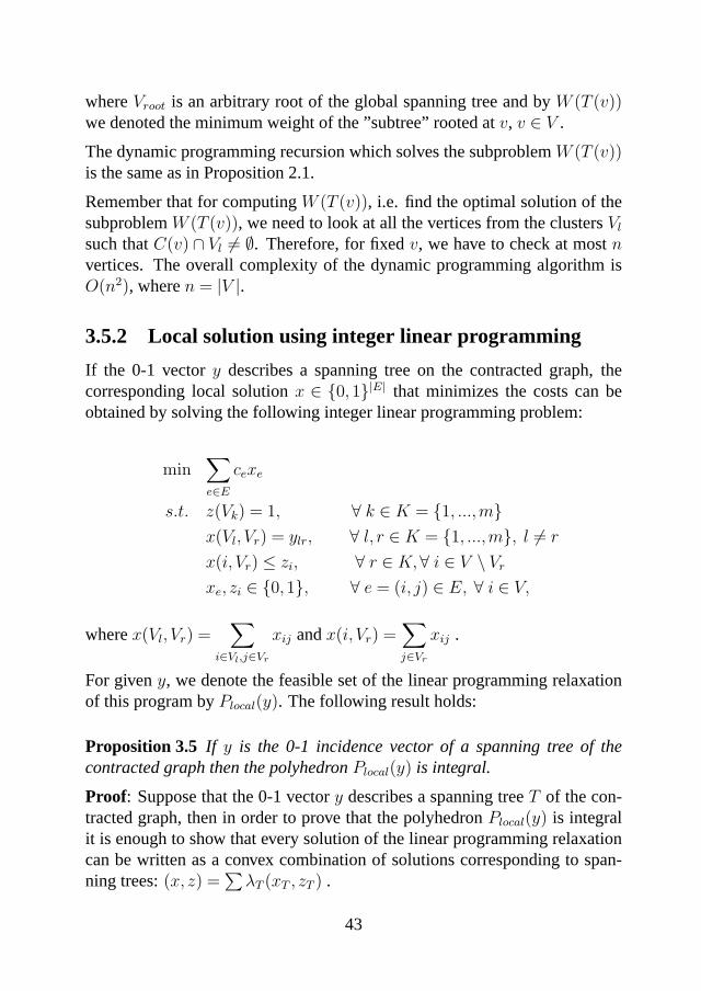
3.5.2 Local solution using integer linear programming
If the 0-1 vectory describes a spanning tree on the contracted graph, thecorresponding local solutionx ∈ {0,1}|E| that minimizes the costs can beobtained by solving the following integer linear programming problem:
min∑e∈E
cexe
s.t. z(Vk) = 1, ∀ k ∈ K = {1, ...,m}x(Vl, Vr) = ylr, ∀ l, r ∈ K = {1, ...,m}, l 6= r
x(i, Vr) ≤ zi, ∀ r ∈ K,∀ i ∈ V \ Vr
xe, zi ∈ {0,1}, ∀ e = (i, j) ∈ E, ∀ i ∈ V,
wherex(Vl, Vr) =∑
i∈Vl,j∈Vr
xij andx(i, Vr) =∑j∈Vr
xij .
For giveny, we denote the feasible set of the linear programming relaxationof this program byPlocal(y). The following result holds:
Proposition 3.5 If y is the 0-1 incidence vector of a spanning tree of thecontracted graph then the polyhedronPlocal(y) is integral.
Proof: Suppose that the 0-1 vectory describes a spanning treeT of the con-tracted graph, then in order to prove that the polyhedronPlocal(y) is integralit is enough to show that every solution of the linear programming relaxationcan be written as a convex combination of solutions corresponding to span-ning trees:(x, z) =
∑λT (xT , zT ) .
43

The proof is by induction on the support of x, denoted bysupp(x) and definedas follows:
supp(x) := {xe | xe 6= 0, e ∈ E}.
Suppose that there is a global connection between the clustersVl andVr (i.e.ylr = 1) then
1 = x(Vl, Vr) =∑i∈Vl
x(i, Vr) ≤∑i∈Vl
zi = 1,
which implies thatx(i, Vr) = zi .
We claim thatsupp(x) ⊆ E contains a tree connecting all clusters. Assumethe contrary and letT 1 ⊆ E be a maximal tree insupp(x). SinceT 1 doesnot connect all clusters, there is some edge(l, r) with ylr = 1 such thatT 1 hassome vertexi ∈ Vl but no vertex inVr. Thenzi > 0, and thusx(i, Vr) = zi > 0,soT 1 can be extended by somee = (i, j) with j ∈ Vr , a contradiction.
Now let xT 1be the incidence vector ofT 1 and letα := min{xe | e ∈ T 1}. If
α = 1, thenx = xT 1and we are done. Otherwise, letzT 1
be the vector whichhaszT 1
i = 1 if T 1 coversi ∈ V andzT 1
i = 0 otherwise. Then
(x, z) := ((1− α)−1(x− αxT 1
), (1− α)−1(z − αzT 1
))
is again inPlocal(y) and, by induction, it can be written as a convex combina-tion of tree solutions. The claim follows.
¤
A similar argument shows that the polyhedronPlocal(y) is integral even inthe case when the 0-1 vectory describes a cycle free subgraph in the con-tracted graph. If the 0-1 vectory contains a cycle of the contracted graph thenPlocal(y) is in general not integral. In order to show this consider the followingexample:
44
2
1
1/2
3
4
5
6
1/2
1/2
1/2
1/2
1/2
1/2
1/2
1/2 1/2
1/2
1/2
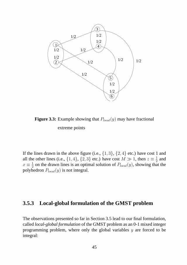
Figure 3.3: Example showing thatPlocal(y) may have fractional
extreme points
If the lines drawn in the above figure (i.e.,{1,3}, {2,4} etc.) have cost 1 andall the other lines (i.e.,{1,4}, {2,3} etc.) have costM À 1, thenz ≡ 1
2and
x ≡ 12
on the drawn lines is an optimal solution ofPlocal(y), showing that thepolyhedronPlocal(y) is not integral.
3.5.3 Local-global formulation of the GMST problem
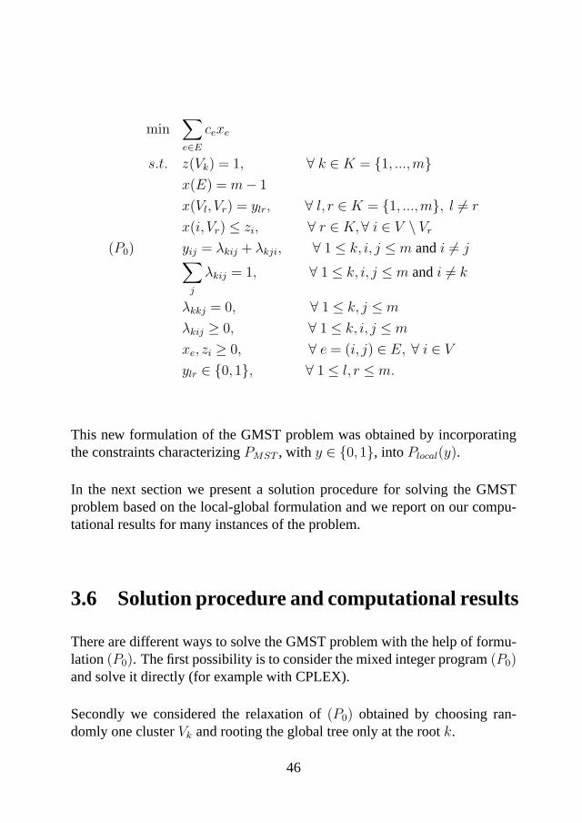
The observations presented so far in Section 3.5 lead to our final formulation,calledlocal-global formulationof the GMST problem as an 0-1 mixed integerprogramming problem, where only the global variablesy are forced to beintegral:
45
min∑e∈E
cexe
s.t. z(Vk) = 1, ∀ k ∈ K = {1, ...,m}x(E) = m− 1
x(Vl, Vr) = ylr, ∀ l, r ∈ K = {1, ...,m}, l 6= r
x(i, Vr) ≤ zi, ∀ r ∈K,∀ i ∈ V \ Vr
(P0) yij = λkij + λkji, ∀ 1 ≤ k, i, j ≤m andi 6= j∑j
λkij = 1, ∀ 1 ≤ k, i, j ≤m andi 6= k
λkkj = 0, ∀ 1 ≤ k, j ≤m
λkij ≥ 0, ∀ 1 ≤ k, i, j ≤m
xe, zi ≥ 0, ∀ e = (i, j) ∈ E, ∀ i ∈ V
ylr ∈ {0,1}, ∀ 1 ≤ l, r ≤m.
This new formulation of the GMST problem was obtained by incorporatingthe constraints characterizingPMST , with y ∈ {0,1}, into Plocal(y).
In the next section we present a solution procedure for solving the GMSTproblem based on the local-global formulation and we report on our compu-tational results for many instances of the problem.
3.6 Solution procedure and computational results
There are different ways to solve the GMST problem with the help of formu-lation(P0). The first possibility is to consider the mixed integer program(P0)and solve it directly (for example with CPLEX).
Secondly we considered the relaxation of(P0) obtained by choosing ran-domly one clusterVk and rooting the global tree only at the rootk.
46

min∑e∈E
cexe
s.t. z(Vk) = 1, ∀ k ∈K = {1, ...,m}x(E) = m− 1
x(Vl, Vr) = ylr, ∀ l, r ∈ K = {1, ...,m}, l 6= r
x(i, Vr) ≤ zi, ∀ r ∈K,∀ i ∈ V \ Vr
(P k0 ) yij = λkij + λkji, ∀ 1 ≤ k, i, j ≤m andi 6= j, k fixed∑
j
λkij = 1, ∀ 1 ≤ k, i, j ≤m andi 6= k, k fixed
λkkj = 0, ∀ 1 ≤ k, j ≤m, k fixed
λkij ≥ 0, ∀ 1 ≤ k, i, j ≤m, k fixed
xe, zi ≥ 0, ∀ e = (i, j) ∈ E, ∀ i ∈ V
ylr ∈ {0,1}, ∀ 1 ≤ l, r ≤m.
If the optimal solution of this relaxation produces a generalized spanning tree,then we have given the optimal solution of the GMST problem. Otherwise wechoose another root or add a second root and proceed in this way till we getthe optimal solution of the GMST problem. We call this procedure therootingprocedure.
It turned out that the lower bounds computed by solving the linear program-ming relaxation of (Pk0) are comparable with the lower bounds given in [54],but can be computed faster.
Upper bounds can be computed by solvingPlocal(y) for certain 0-1 vectorycorresponding to a spanning tree. (E.g., a minimum spanning tree w.r.t. theedge weightsdlr = min{cij | i ∈ Vl, j ∈ Vr}.)We compare the computational results for solving the problem using our root-ing procedure with the computational results given by Myunget al. in [54].
According to the method of generating the edge costs, the problems generatedare classified into three types:
• structured Euclidean case
• unstructured Euclidean case
47

• non-Euclidean case
For the instances in the structured Euclidean casem squares (clusters) are”packed in a square” and in each of thesem clustersnc nodes are selectedrandomly. The costs between nodes are the Euclidean distances between thenodes. So in this model the clusters can be interpreted as physical clusters. Inthe other models such an interpretation is not valid.
For the unstructured Euclidean casen = mnc nodes are generated randomly in[0,100]2 with costs given by the Euclidean distances. But then the clusters arechoosen randomly among these points. Finally in the non-Euclidean modelthe edge costs are randomly generated on[0,100].
Our algorithms have been coded in C and compiled with a HP-UX cc com-piler. For solving the linear and mixed integer programming problems weused CPLEX. The computational experiments were performed on a HP 9000/735computer with a 125 Mhz processor and 144 Mb memory.
Tables 3.1, 3.2 and 3.3 show the computational results for the non-Euclidean,unstructured Euclidean and structured Euclidean problems.
48

Table 3.1: Computational Results for non-Euclidean problems(average of five problems for each combination)
Pb. size Rooting Procedure Myung’s results [54]m nc LB/OPT roots iter. CPU LB/OPT LB/UB CPU
8 3 100 1 1 0.07 100 - 0.054 100 1 1 0.09 96.1 - 0.576 100 1 1 0.14 94.3 - 3.2510 100 1 1 0.69 94.9 - 17.68
10 3 100 1 1 0.10 89.1 - 0.054 100 1 2 0.32 99.2 - 2.136 100 1 1 0.76 87.8 - 3.2510 100 1 1 3.53 91.3 - 17.68
12 3 100 1 1 0.17 89.6 - 6.004 100 1 1 0.21 92.8 - 7.636 100 2 3 5.61 91.3 - 54.9810 100 1 2 14.57 - - -
15 3 100 1 1 0.29 89.0 - 17.454 100 1 1 0.73 - - -6 100 1 1 5.99 - 86.2 7.6510 100 2 2 40.53 - 82.7 18.25
18 3 100 1 1 0.57 95.3 - 38.836 100 1 1 9.45 - - -10 100 1 2 193.81 - - -
20 3 100 2 3 3.82 - - -6 100 1 1 1.46 - 81.4 13.710 100 1 2 407.64 - 77.5 35.8
25 3 100 1 2 21.68 - - -6 100 1 1 25.12 - 80.5 44.48 100 1 2 306.69 - 81.0 76.8
30 3 100 1 1 4.01 - - -6 100 2 2 84.05 - 74.3 45.28 100 1 1 341.16 - - -
40 3 100 2 3 71.64 - 84.1 36.54 100 1 2 1713.29 - 74.9 154.8
49

Table 3.2: Computational Results for structured Euclidean problems(average of five problems for each combination)
Pb. size Rooting Procedure Myung’s results [54]m nc LB/OPT roots iter. CPU LB/OPT LB/UB CPU
8 3 100 1 1 0.05 - - -4 100 2 3 0.09 - - -6 100 2 3 0.15 - - -10 100 2 3 0.85 - - -
10 3 100 2 3 0.06 - - -4 100 3 4 0.20 - - -6 100 3 4 0.54 - - -10 100 3 4 2.39 - - -
12 3 100 2 3 0.21 - - -4 100 3 4 0.42 - - -6 100 3 4 1.12 - - -10 100 3 4 5.43 - - -
15 3 100 3 4 0.72 - - -4 100 3 4 0.95 - - -6 100 4 5 3.80 - - -8 100 4 5 29.73 - - -
18 3 100 4 5 1.68 - - -6 100 4 5 18.25 - - -8 100 4 5 55.24 - - -
20 3 100 4 5 3.70 - - -6 100 5 6 20.18 - - -8 100 5 6 97.31 - - -
25 3 100 4 5 18.67 - - -6 100 4 5 198.63 - - -8 100 4 5 325.76 - - -
30 3 100 4 5 46.34 - - -4 100 4 5 51.33 - - -6 100 4 5 301.86 - - -
40 3 100 4 5 141.28 - - -4 100 4 5 283.72 - - -
50
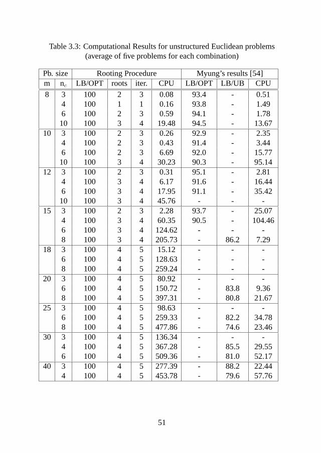
Table 3.3: Computational Results for unstructured Euclidean problems(average of five problems for each combination)
Pb. size Rooting Procedure Myung’s results [54]m nc LB/OPT roots iter. CPU LB/OPT LB/UB CPU
8 3 100 2 3 0.08 93.4 - 0.514 100 1 1 0.16 93.8 - 1.496 100 2 3 0.59 94.1 - 1.7810 100 3 4 19.48 94.5 - 13.67
10 3 100 2 3 0.26 92.9 - 2.354 100 2 3 0.43 91.4 - 3.446 100 2 3 6.69 92.0 - 15.7710 100 3 4 30.23 90.3 - 95.14
12 3 100 2 3 0.31 95.1 - 2.814 100 3 4 6.17 91.6 - 16.446 100 3 4 17.95 91.1 - 35.4210 100 3 4 45.76 - - -
15 3 100 2 3 2.28 93.7 - 25.074 100 3 4 60.35 90.5 - 104.466 100 3 4 124.62 - - -8 100 3 4 205.73 - 86.2 7.29
18 3 100 4 5 15.12 - - -6 100 4 5 128.63 - - -8 100 4 5 259.24 - - -
20 3 100 4 5 80.92 - - -6 100 4 5 150.72 - 83.8 9.368 100 4 5 397.31 - 80.8 21.67
25 3 100 4 5 98.63 - - -6 100 4 5 259.33 - 82.2 34.788 100 4 5 477.86 - 74.6 23.46
30 3 100 4 5 136.34 - - -4 100 4 5 367.28 - 85.5 29.556 100 4 5 509.36 - 81.0 52.17
40 3 100 4 5 277.39 - 88.2 22.444 100 4 5 453.78 - 79.6 57.76
51

The first two columns in the tables give the number of clusters (m) and thenumber of nodes per cluster (nc). The next four columns describe our rootingprocedure and contain: (LB/OPT) the lower bounds obtained as a percentageof the optimal value of the GMST problem, (roots) the number of root clustersand (iter.) the number of mixed integer programs necessary to find the optimalsolution and (CPU) the computation time in seconds for solving the GMSTproblem to optimality. The last columns give the numerical results reportedby Myunget al. in [54]. The numerical results in [54] were obtained basedon the dual of the linear programming relaxation of the multicommodity flowformulation. These columns evaluate the lower bounds obtained as a percent-age of the optimal objective value, respectively the lower bounds obtained asa percentage of the upper bounds and finally the computation time is shownin the last column. In the last three columns ’-’ means that this information isnot provided in [54].
As can be seen, in all the problems that we considered, the optimal solutionof the GMST problem has been found by using our rooting procedure. Thesenumerical experiences with the new formulation of the GMST problem arevery promising.
The computational results so far could indicate that the exponential growthof the computation time for solving the GMST problem to optimality is mod-erate in comparison with the growth of computation time for solving the fullproblem directly, for example with CPLEX.
Finishing the thesis we became aware of the branch and cut numerical resultsprovided by Feremans [17]. In comparison with our numerical results, in[17] in about 75% of the considered instances the optimal value of the GMSTproblem is obtained, but the computing times spent by the branch and cutcode are in general larger than the times spent by the rooting procedure code.
3.7 Concluding remarks
We have provided several integer and mixed integer programming formula-tions for the GMST problem and established relationships between the poly-topes of their linear relaxations.
Based on one of the new formulations that we introduced, i.e. the local-global formulation of the GMST problem, we present a new solution pro-cedure called rooting procedure. Computational results show that the rooting
52

procedure performs better in comparison with earlier methods. For all the in-stances of the problem that we considered, the optimal solution of the GMSTproblem has been found by using our solution procedure.
53


Chapter 4
Approximation Algorithms
Throughout this chapter we will distinguish between so-calledpositive re-sults which establish the existence of some approximation algorithms, andso-callednegative resultswhich disprove the existence of good approximationresults for some combinatorial optimization problems under the assumptionthatP 6= NP.
We start with some basic results of the approximation theory. In Section 4.2we focus on positive results in the area of approximation: design and analysisof polynomial time approximation algorithms. We present in Section 4.3 anin-approximability result for the GMST problem. Finally, in the last section ofthis chapter, under special assumptions, we give an approximation algorithmfor the GMST problem with bounded cluster size. Roughly, the last sectioncan be found in Pop, Kern and Still [62].
55

The basic results presented in the first two sections follow the descriptions ofGoemans [27] and Schuurman and Woeginger [70].
4.1 Introduction
Many of the optimization problems we would like to solve areNP-hard.Therefore it is very unlikely that these problems could be solved by a polyno-mial-time algorithm. However, these problems still have to be solved in prac-tice. In order to do that, we have to relax some of the requirements. There arein general, three different possibilities.
• Superpolynomial-time algorithms: Even though an optimization prob-lem isNP-hard, there are ”good” and ”not so good” algorithms forsolving it exactly. To the ”not so good” algorithms certainly belongmost of the simple enumeration methods where one would enumerateall the feasible solutions and then choose the one with the optimal valueof the objective function. Such methods have very high time complex-ity. Among the ”good” algorithms belong methods likebranch-and-boundwhere an analysis of the problem at hand is used to discard mostof the feasible solutions before they are even considered. These ap-proaches allow one to obtain exact solutions of reasonably large prob-lem instances, but their running time still depends exponentially on thesize of the problem.
• Average-case polynomial-time algorithms: For some problems, itis possible to have algorithms which require superpolynomial-time ononly a few instances and for the other instances run in polynomial time.A famous example is theSimplex Methodfor solving problems in Lin-ear Programming.
• Approximation Algorithms: We may also relax the requirement ofobtaining an exact solution of the optimization problem and contentourselves with a solution which is ”not too far” from the optimum. Thisis partially justified by the fact that, in practice, it is usually enough toobtain a solution that is slightly sub-optimal.
Clearly, there are good approximation algorithms and bad ones as well. Whatwe need is some means of determining the quality of an approximation algo-
56
rithm and a way of comparing different algorithms. There are a few criteriato consider:
Average-case performance:One has to consider some probability distribu-tion on the set of all possible instances of a given problem. Based on thisassumption, an expectation of the performance can then be found. Results ofthis kind strongly depend on the choice of the initial distribution and do notprovide us any information about the performance on a particular instance.
Experimental performance: This approach is based on running the algo-rithm on a few ”typical” instances. It has been used mostly to compare per-formance of several approximation algorithms. Of course the result dependon the choice of the ”typical” instances and may vary from experiment toexperiment.
Worst-case performance: This is usually done by establishing upper andlower bounds for approximate solutions in terms of the optimum value. Incase of minimization problems, we try to establish upper bounds, in case ofmaximization problems, one wants to find lower bounds.
The advantage of the worst-case bounds on the performance of approximationalgorithms is the fact that given any instance of the optimization problem, weare guaranteed that the approximate solution stays within these bounds. Itshould also be noted that approximation algorithms usually output solutionsmuch closer to the optimum than the worst-case bounds suggest. Thus it isof independent interest to see how tight the bounds on the performance ofeach algorithm are; that is, how bad the approximate solution can really get.This is usually done by providing examples of specific instances for whichthe approximate solution is very far from the optimum solution.
Establishing worst-case performance bounds for even simple algorithms of-ten requires a very deep understanding of the problem at hand and the useof powerful theoretical results from areas like linear programming, combina-torics, graph theory, probability theory, etc.
We consider anNP-hard optimization problem for which as we have seenit is difficult to find the exact optimal solution within polynomial time. Atthe expense of reducing the quality of the solution by relaxing some of therequirements, we can often get considerable speed-up in the complexity. Thisleads us to the following definition:
Definition 4.1 (Approximation algorithms)Let X be a minimization problem andα > 1. An algorithmAPP is called
57

an α-approximation algorithm for problemX, if for all instancesI of X itdelivers in polynomial time a feasible solution with objective valueAPP (I)such that
APP (I) ≤ αOPT (I), (4.1)
where byAPP (I) and OPT (I) we denoted the values of an approximatesolution and that of an optimal solution for instanceI, respectively.
¤
The valueα is called theperformance guaranteeor theworst case ratioof theapproximation algorithmAPP . The closerα is to 1 the better the algorithmis.
4.2 Positive Results: the Design of the Approxi-mation Algorithms
Positive results in the area of approximation concern the design and analysisof polynomial time approximation algorithms. This section concentrates onsuch positive results; we will outline the main strategy.
Assume that we need to find an approximation algorithm for anNP-hardop-timization problemX. How shall we proceed? We will concentrate on min-imization problems, but the ideas apply equally well to maximization prob-lems.
In what follows, given an instanceI of an optimization problem and some al-gorithm for its approximation, we will denote byOPT = OPT (I) the valueof an optimum solution and byAPP = APP (I) the value of the solution out-put by the approximation algorithm. We are interested in anα-approximationalgorithm, i.e. an algorithmAPP such that
APP ≤ αOPT.
RelatingAPP to OPT directly can be difficult. Therefore instead we tryto find a lower bound denoted byLB for the optimal solution satisfying thefollowing conditions:
1. LB ≤ OPT
58

2. APP ≤ αLB.
Consider now the following optimization problem:
OPT = minx∈S
f(x).
A lower bound onOPT can be obtained by so-calledrelaxation. Considerthe following related optimization problem:
LB = minx∈R
g(x).
Definition 4.2 (Lower bound)
LB is called a lower bound onOPT and the optimization problem is calleda relaxation of the original problem if the following two conditions hold:
S ⊆ R
g(x) ≤ f(x) for all x ∈ S.
¤
The above conditions imply the following:
LB = minx∈R
g(x) ≤ minx∈S
f(x) = OPT.
showing thatLB is a lower bound onOPT .
Many combinatorial optimization problems can be formulated as integer ormixed integer programs and the linear programming relaxations of this pro-grams provide a lower bound for the optimal solution. Later we show how touse a linear programming relaxation of an integer programming formulationof the GMST problem to get anα-approximation algorithm for the GMSTproblem with bounded cluster size.
There are two main techniques to derive an approximately optimal solutionfrom a solution of the relaxed problem:
1. Rounding
59
The idea is to solve the linear programming relaxation and then convert thefractional solution obtained into an integral solution. The approximation guar-antee is establish by comparing the costs of the integral and fractional solu-tions.
Therefore we find an optimal solutionx∗ to the relaxation and ”round”x∗ ∈Rto an elementx
′ ∈ S. Then prove thatf(x′) ≤ αg(x∗) which implies that
f(x′) ≤ αLB ≤ αOPT.
Often randomization is helpful. In this casex∗ ∈ R is randomly roundedto some elementx
′ ∈ S so thatE[f(x′)] ≤ αg(x∗). These algorithms can
sometimes be derandomized, in which case one finds anx′′
such thatf(x′′)≤
E[f(x′)].
An example where the rounding technique is applied, is the Minimum WeightVertex Cover Problem, result due to Hochbaum [38].
2. Primal-Dual
We consider the linear programming relaxation of the primal program. Thismethod constructs iteratively an integer solution to the primal program and afeasible solution to the dual program,max{h(y) : y ∈ D}. The approxima-tion guarantee is establish by comparing the two solutions.
The weak duality property of the relaxation implies:
max{h(y) : y ∈ D} ≤min{g(x) : x ∈ R}We constructx ∈ S from y ∈ D such that:
f(x) ≤ αh(y) ≤ αh(ymax) ≤ αg(xmin) ≤ αOPT.
Notice thaty can be any element ofD, not necessarily an optimal solution tothe dual.
More details about primal-dual technique can be found in [1] and [75].
4.3 A negative result for the GMST problem
For some hard combinatorial optimization problems it is possible to showthat they don’t have an approximation algorithm unlessP = NP . In order
60

to give a result of this form it is enough to show that the existence of anα-approximation algorithm would allow one to solve some decision problem,known to beNP-complete, in polynomial time.
Applying this scheme to the GMST problem we obtain an in-approximabilityresult. This result is a different formulation in terms of approximation algo-rithms of a result provided by Myunget al. [54] which says that even findinga near optimal solution for the GMST problem isNP-hard. Our proof isslightly different to the proof provided in [54].
Theorem 4.1 Under the assumptionP 6= NP, there is noα-approximationalgorithm for the GMST problem.
Proof: Assume that there exists anα-approximation algorithmAPP for theGMST problem, whereα is a real number greater than or equal to 1. Thismeans that
APP (I) ≤ αOPT (I),
for every instanceI, whereOPT (I) andAPP (I) are the values of the opti-mal solution and of the solution found by the algorithmAPP , respectively.
Then, we will show thatAPP also solves the node-cover problem for a givengraphG = (V,E) and an integerk such thatk < |V |. This result contradictsthe assumption thatP 6= NP.
We construct a graphG′= (V
′,E
′) and the edge cost function such that the
algorithmAPP finds a feasible solution with a value no greater thanα timesthe optimal cost if and only if G contains C, whereC is a node cover ofG,i.e. a subset ofV such that all the edges ofG are adjacent to at least one nodeof C.
The graphG′
contains the followingm = |E| + k + 1 node sets (clusters),V′1 , ..., V
′m:
• V′1 consists of a single node denoted byr,
• V′2 , ..., V
′k+1 are identical node sets, each of which has|V | nodes corre-
sponding to the nodes ofV , and
• |E| node sets,V′k+2, ..., V
′m, each of which contains a single node corre-
sponding to an edgee ∈ E.
61
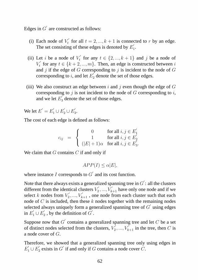
Edges inG′are constructed as follows:
(i) Each node ofV′t for all t = 2, ..., k + 1 is connected tor by an edge.
The set consisting of these edges is denoted byE′1.
(ii) Let i be a node ofV′t for any t ∈ {2, ..., k + 1} and j be a node of
V′t for any t ∈ {k + 2, ...,m}. Then, an edge is constructed betweeni
andj if the edge ofG corresponding toj is incident to the node ofGcorresponding toi, and letE
′2 denote the set of those edges.
(iii) We also construct an edge betweeni andj even though the edge ofGcorresponding toj is not incident to the node ofG corresponding toi,and we letE
′3 denote the set of those edges.
We letE′= E
′1 ∪E
′2 ∪E
′3.
The cost of each edge is defined as follows:
cij =
0 for all i, j ∈ E′1
1 for all i, j ∈ E′2
(|E|+ 1)α for all i, j ∈ E′3.
We claim thatG containsC if and only if
APP (I) ≤ α|E|,where instanceI corresponds toG
′and its cost function.
Note that there always exists a generalized spanning tree inG′: all the clusters
different from the identical clustersV′2 , ..., V
′k+1 have only one node and if we
selectk nodes fromV′2 , ..., V
′k+1 , one node from each cluster such that each
node ofC is included, then thesek nodes together with the remaining nodesselected always uniquely form a generalized spanning tree ofG
′using edges
in E′1 ∪E
′2 , by the definition ofG
′.
Suppose now thatG′contains a generalized spanning tree and letC be a set
of distinct nodes selected from the clusters,V′2 , ..., V
′k+1 in the tree, thenC is
a node cover ofG.
Therefore, we showed that a generalized spanning tree only using edges inE′1 ∪E
′2 exists inG
′if and only if G contains a node coverC.
62

If G containsC, thenOPT (I) = |E|. Moreover, ifG does not containC,then any generalized spanning tree ofG
′should use at least one edge inE
′3
and thus
OPT (I) ≥ |E| − 1 + α(|E|+ 1) > α|E|.In particular ifG contains a node coverC then the approximation algorithmAPP will produce a solution with value
APP (I) ≤ α|E| = αOPT (I),
i.e. the solution does not use any edge fromE′3 andAPP identifies a node
cover.¤
However, under further assumptions, in the next section we present a positiveresult for the GMST problem.
4.4 An Approximation Algorithm for BoundedCluster Size
As we have seen in the previous section there exists noα-approximation al-gorithm for the GMST problem under the assumptionP 6= NP.
However under the following assumptions:
A1: the graph has bounded cluster size, i.e.|Vk| ≤ ρ, for all k = 1, ...m
A2: the cost function is strict positive and satisfies the triangle inequality,i.e. cij + cjk ≥ cik for all i, j, k ∈ V ,
a polynomial approximation algorithm for the GMST problem is possible.
In this section under the above assumptions we present an approximation al-gorithm for the GMST problem with performance ratio 2ρ. The approxima-tion algorithm is constructed following the ideas of Slavik [71] where theGeneralized Traveling Salesman Problem and Group Steiner Tree Problemhave been treated.
63
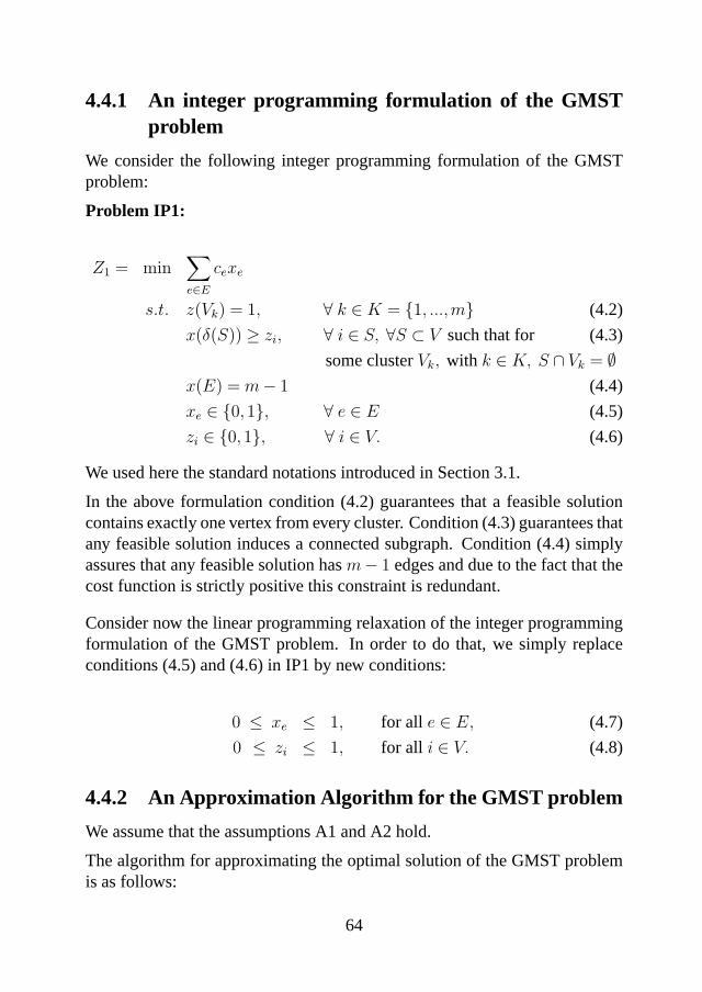
4.4.1 An integer programming formulation of the GMSTproblem
We consider the following integer programming formulation of the GMSTproblem:
Problem IP1:
Z1 = min∑e∈E
cexe
s.t. z(Vk) = 1, ∀ k ∈ K = {1, ...,m} (4.2)
x(δ(S)) ≥ zi, ∀ i ∈ S, ∀S ⊂ V such that for (4.3)
some clusterVk, with k ∈ K, S ∩ Vk = ∅x(E) = m− 1 (4.4)
xe ∈ {0,1}, ∀ e ∈ E (4.5)
zi ∈ {0,1}, ∀ i ∈ V. (4.6)
We used here the standard notations introduced in Section 3.1.
In the above formulation condition (4.2) guarantees that a feasible solutioncontains exactly one vertex from every cluster. Condition (4.3) guarantees thatany feasible solution induces a connected subgraph. Condition (4.4) simplyassures that any feasible solution hasm− 1 edges and due to the fact that thecost function is strictly positive this constraint is redundant.
Consider now the linear programming relaxation of the integer programmingformulation of the GMST problem. In order to do that, we simply replaceconditions (4.5) and (4.6) in IP1 by new conditions:
0 ≤ xe ≤ 1, for all e ∈ E, (4.7)
0 ≤ zi ≤ 1, for all i ∈ V. (4.8)
4.4.2 An Approximation Algorithm for the GMST problem
We assume that the assumptions A1 and A2 hold.
The algorithm for approximating the optimal solution of the GMST problemis as follows:
64

Algorithm ”Approximate the GMST problem”
Input: A complete graphG = (V,E) with strictly positive cost functionon the edges satisfying the triangle inequality, and with the nodespartitioned into the clustersV1, ..., Vm with bounded size,|Vk| ≤ ρ.
Output: A treeT ⊂ G spanning some verticesW′ ⊂ V which includes ex-
actly one vertex from every cluster, that approximates the optimalsolution to the GMST problem.
1. Solve the linear programming relaxation of the problem IP1 and let(z∗, x∗,Z∗1 ) = ((z∗i )n
i=1, (x∗e)e∈E ,Z∗1 ) be the optimal solution.
2. SetW ∗ ={
i ∈ V |z∗i ≥ 1ρ
}and considerW
′ ⊂ W ∗, with the prop-
erty thatW′
has exactly one vertex from each cluster, and find aminimum spanning treeT ⊂ G on the subgraphG
′generated by
W′.
3. OutputAPP = cost(T ) and the generalized spanning treeT .
Even though the linear programming relaxation of the problem IP1 has ex-ponentially many constraints, it can still be solved in polynomial time ei-ther using the ellipsoid method with a min-cut max-flow oracle [32] or usingKarmarkar’s algorithm [42] since the linear programming relaxation can beformulated ”compactly” (the number of constraints polynomially bounded)using flow variables see Section 3.4.
4.4.3 Auxiliary results
We start this subsection with a result established by Goemans and Bertsimas[29] and calledparsimonious property.
Given a complete undirected graphG = (V,E). We associate with each edge(i, j) ∈E a costcij and for any pair(i, j) of vertices, letrij be the connectivityrequirement betweeni andj (rij is assumed to be symmetric, i.e.rij = rji).A network is calledsurvivableif it has at leastrij edge disjoint paths betweenany pair(i, j) of vertices.
Thesurvivable network design problemconsists in finding the minimum cost
65
survivable network. This problem can be formulated by the following integerprogram:
(IP∅(r)) IZ∅(r) = min∑e∈E
cexe
s.t. x(δ(S)) ≥ max(i,j)∈δ(S)
rij, S ⊂ V, S 6= ∅ (4.9)
0 ≤ xe, e ∈ E,
xe integral, e ∈ E.
We denote byIZ∅(r) the optimal value of the above integer program. Let(P∅(r)) denote the linear programming relaxation of(IP∅(r)) obtained bydropping the integrality restrictions and letZ∅(r) be its optimal value.
By definition the degree of vertexi ∈ V is dx(i) = x(δ(i)), for any feasiblesolutionx, either to(IP∅(r)) or to (P∅(r)). Because of constraints (4.9) forS = {i}, the degree of vertexi is at least equal tomax
j∈V \{i}rij. If dx(i) =
maxj∈V \{i}
rij , then we say thatx is parsimoniousat vertexi. If we impose
that the solutionx is parsimonious at all the vertices of a setD ⊆ V , we getsome interesting variations of(IP∅(r)) and(P∅(r)), denoted by(IPD(r)) and(PD(r)) respectively. The formulation of(IPD(r)) as an integer program is:
(IPD(r)) IZD(r) = min∑e∈E
cexe
s.t. x(δ(S)) ≥ max(i,j)∈δ(S)
rij, S ⊂ V, S 6= ∅x(δ(i)) = max
j∈V \{i}rij, i ∈ D, D ⊆ V
0 ≤ xe, e ∈ E
xe integral, e ∈ E.
We denote byIZD(r) the optimal value of the above integer program. Let(PD(r)) denote the linear programming relaxation of(IPD(r)) obtained bydropping the integrality restrictions and letZD(r) be its optimal value.
Theorem 4.2 (parsimonious property, Goemans and Bertsimas [29])If the costscij satisfy the triangle inequality, then
Z∅(r) = ZD(r)
66
for all subsetsD ⊆ V. ¤
The proof of this theorem is based on a result on connectivity properties ofEulerian multigraphs, due to Lovasz [50].
Let nowW ⊂ V and consider the following linear program:
Problem LP2:
Z∗2(W ) = min
∑e∈E
cexe
s.t. x(δ(S)) ≥ 1, S ⊂ V, s.t.W ∩ S 6= ∅ 6= W \ S(4.10)
x(δ(i)) = 0, i ∈ V \W, (4.11)
0 ≤ xe ≤ 1, e ∈ E. (4.12)
Replacing constraints (4.12) with the integrality constraintsxe ∈ {0,1}, theformulation obtained is the formulation of the minimum tree spanning thesubset of nodesW ⊂ V .
Consider the following relaxation of the problem LP2.
Problem LP3:
Z∗3(W ) = min
∑e∈E
cexe
s.t. x(δ(S)) ≥ 1, S ⊂ V, s.t.W ∩ S 6= ∅ 6= W \ S
0 ≤ xe, e ∈ E. (4.13)
Thus we omitted constraint (4.11) and relaxed constraint (4.12).
The following result is a straightforward consequence of the parsimoniusproperty, if we chooserij = 1, if i, j ∈W , and 0 otherwise, andD = V \W .
Lemma 4.1 The optimal solution values to problems LP2 and LP3 are thesame, that is
Z∗2(W ) = Z∗
3(W ).
¤
67
Consider the following problem:
Problem IP4:
Z4 = min∑e∈E
cexe
s.t. x(δ(S)) ≥ 1, S ⊂ V, s.t.S 6= ∅ 6= V (4.14)
xe ∈ {0,1}, e ∈ E. (4.15)
Clearly, it is the integer programming formulation of the MST (minimumspanning tree) problem. Let LP4 be the LP relaxation of this formulation,that is, we simply replace the constraint (4.15) by the constraint0 ≤ xe ≤ 1,for all e ∈ E.
Denote byZ∗4 the value of the optimal solution of the LP4. The following
known result for minimum spanning trees holds:
Proposition 4.1
LT (V ) ≤ (2− 2
|V |)Z∗4 ,
whereLT (V ) denotes the cost of the minimum spanning tree on V.
Proof: See for example [71]. ¤
Let W ⊂ V , then Proposition 4.1 can be easily modified to obtain:
Proposition 4.2
LT (W ) ≤ (2− 2
|W |)Z∗2(W ).
Proof: Let (xe) be a feasible solution to LP2. Ife /∈ E(W ) = {(i, j) | i, j ∈W} impliesxe = 0 and using Proposition 4.1 we prove the inequality. ¤
4.4.4 Performance Bounds
Let (z∗, x∗,Z∗1) = ((z∗i )
ni=1, (x
∗e)e∈E,Z∗
1) be the optimal solution to the linearprogramming relaxation of the GMST problem. Define
xe = ρx∗e
68

zi =
1 if z∗i ≥1
ρ
0 otherwise.
W ∗ =
{i ∈ V | z∗i ≥
1
ρ
}= {i ∈ V | zi = 1}. Because we need only one
vertex from every cluster we delete extra vertices fromW ∗ and considerW
′ ⊂ W ∗ such that|W ′| = m andW′
consists of exactly one vertex fromevery cluster.
Since LP1 is the linear programming relaxation of the problem IP1, we have
Z∗1 ≤ Z1.
Now let us show that(xe)e∈E is a feasible solution to LP3 withW = W′.
Indeed,xe ≥ 0 for all e ∈ E, hence condition (4.13) is satisfied. LetS ⊂ Vbe such thatW
′ ∩ S 6= ∅ 6= W′ \ S and choose somei ∈W
′ ∩ S. Hencezi =1 andz∗i ≥ 1
ρ. Then we have
x(δ(S)) =∑
e∈δ(S)
xe = ρ∑
e∈δ(S)
x∗e ≥ ρz∗i ≥ ρ1
ρ= 1,
by definition ofxe and the fact that the(x∗e) solve LP1. Hence the(xe) satisfyconstraint (4.10) in LP3.
Therefore, for the algorithmAPP on page 65
APP = LT (W′) ≤ (2− 2
|W ′|)Z∗2(W
′) = (2− 2
|W ′|)Z∗3(W
′)
≤ (2− 2
|W ′ |)∑e∈E
cexe = (2− 2
|W ′|)ρ∑e∈E
cex∗e = (2− 2
|W ′|)ρZ∗1
≤ (2− 2
|W ′ |)ρZ1 = (2− 2
|W ′|)ρOPT.
And sinceW′ ⊂ V , that is, m =|W ′| ≤ |V | = n, we have proved the following.
69

Theorem 4.3 The performance ratio of the algorithm ”Approximate GMSTproblem” for approximating the optimum solution to the GMST problem sat-isfies:
APP
OPT≤ (2− 2
n)ρ.
¤
In what follows we generalize the algorithm ”Approximate GMST problem”and its analysis to the case when, in addition to the costcij associated witheach edgee = (i, j) ∈ E, there is a cost, saydi , associated with each vertexi ∈ V .
In this case the GMST problem can be formulated as the following integerprogram:
OPT = min∑e∈E
cexe +∑i∈V
dizi
s.t. (4.2)− (4.6).
Suppose that(x, z) is an optimal solution. Then the optimal valueOPT ofthis integer program consists of two parts:
LOPT :=∑e∈E
cexe andVOPT :=∑i∈V
dizi.
Under the same assumptions A1 and A2, the algorithm for approximating theoptimal solution of the GMST problem in this case, is as follows:
1. Solve the linear programming relaxation of the previous integer pro-gram and let(z∗, x∗) = ((z∗i )n
i=1, (x∗e)e∈E) be the optimal solution.
2. SetW ∗ ={
i ∈ V |z∗i ≥ 1ρ
}and considerW
′ ⊂ W ∗ with the prop-
erty thatW′
has exactly one vertex from each cluster, and find aminimum spanning treeT ⊂ G on the subgraphG
′generated by
W′.
3. OutputAPP = ecost(T ) + vcost(T ) and the generalized spanningtreeT .
70

where byecost(T ) andvcost(T ) we denoted the cost of the treeT with re-spect to the edges, respectively to the nodes.
Regarding the performance bounds of this approximation algorithm, using thesame auxiliary results and defining(xe, zi) as we did at the beginning of thissubsection, the following inequalities hold:
LT (W′) ≤ ρ(2− 2
n)LOPT ,
V T (W′) ≤ ρVOPT ,
whereLT (W′), V T (W
′) denote the cost of the treeT spanning the nodes of
W′
with respect to the edges, respectively to the nodes and as beforeW′ ⊂
W ∗ =
{i ∈ V | z∗i ≥
1
ρ
}, such that|W ′| = m andW
′consists of exactly one
vertex from every cluster.
For the approximation algorithm proposed in this case, the following holds:
APP = LT (W′) + V T (W
′) ≤ ρ(2− 2
n)LOPT + ρVOPT
≤ ρ(2− 2
n)(LOPT + VOPT ) = ρ(2− 2
n)OPT.
4.5 Concluding remarks
We have distinguished between so-called positive results and negative resultsin the area of approximation algorithms.
We presented an in-approximability result: there is noα-approximation al-gorithm for the GMST problem unlessP = NP. However, under specialassumptions (see Section 4.4) we give an approximation algorithm for theGMST problem.
71


Chapter 5
Linear Programming, Lagrangianand Semidefinite Relaxations
As was remarked in Chapter 1 of this thesis, finding good solutions for hardminimization problems in combinatorial optimization requires the considera-tion of two issues:
• calculation of an upper bound that is as close as possible to the opti-mum;
• calculation of a lower bound that is as close as possible to the optimum.
General techniques for generating good upper bounds are essentially heuristicmethods which we are going to consider in Chapter 7 of the thesis. In addition,for any particular problem, we may well have techniques which are specificto the problem being solved.
To obtain lower bounds, one well-known technique is Linear Programming(LP) relaxation. In LP relaxation we take an integer (or mixed-integer) pro-gramming formulation of the problem and relax the integrality requirementon the variables. This gives a linear program which can either be:
• solved exactly using a standard algorithm (simplex or interior point); or
• solved heuristically (dual ascent).
The solution value obtained for this linear program gives a lower bound onthe optimal value of the original minimization problem.
73

Another well-known technique to find lower bounds is Lagrangian relaxation.The general idea is to ”relax” (dualize) some (or all) constraints by addingthem to the objective function using Lagrangian multipliers. Choosing valuesfor the Lagrangian multipliers is of key importance in terms of quality of thelower bound generated.
Semidefinite programming (SDP) is currently a very exciting and active areaof research. Combinatorial optimization problems often involve binary (0,1 or+1,-1) decision variables. These can be modelled using quadratic constraintsx2 − x = 0, andx2 = 1, respectively. Using the positive semidefinite matrixrelationshipX = xxT , we can lift the problem into matrix space and obtaina Semidefinite Programming Relaxation by ignoring the rank 1 restriction onX, see e.g. [49]. These semidefinite relaxations provide tight bounds formany classes of hard problems and in addition can be solved efficiently byinterior-point methods.
74
5.1 Lagrangian Relaxation
5.1.1 Basic principles
The description of this section follows the presentations of Bertsimas andTsitsiklis [5] and Faigleet al. [16].
We consider the following optimization problem:
z∗1 = min {f(x) | g(x) ≤ 0, h(x) ≤ 0, x ∈ X} (5.1)
Dualizing the constraintsg(x) ≤ 0 with Lagrangian multipliersλ, λ ≥ 0,yields the lower bound forz∗1
L(λ) = minx∈X
{f(x) + λT g(x) | h(x) ≤ 0}. (5.2)
Here the functionL (function of λ) is calledLagrangian dual function(orjust dual function). Since the dual function is the pointwise minimum of afamily of affine functions,L(λ) is concave, even when the problem (5.1) isnot convex.
The best bound of this type arises from the solution of theLagrangian dualproblem
maxλ≥0
L(λ). (5.3)
The difference between the optimal value of problems (5.1) and (5.3) is calledduality gap, which is always a nonnegative number. We prove this last resultin Theorem 5.1, in the special case of integer linear programming.
The crucial question is which constraints to dualize. The more constraintsare dualized, the weaker the bound becomes. On the other hand, dualizingmore constraints facilitates the computation ofL(λ). In the extreme case, ifall constraints are dualized, the computation ofL(λ) has no side constraintsto consider. There is a trade off between the quality of the bounds we obtainand the effort necessary for their computation. Generally, one would dualizeonly the ”nasty” constraints, i.e. those that are difficult to deal with directly.
Held and Karp [33], [34] were the first to apply the idea of Lagrangian relax-ation to integer linear programs. Assume we are given an integer program ofthe form
75

z∗IP = min {cT x | Ax ≥ b, Bx ≥ d, x ∈ Zn} (5.4)
for given integral matrices A, B and vectors b, c, d and letz∗IP be the optimumvalue of (5.4). Dualizing the constraintsb−Ax ≤ 0 with multipliersu ≥ 0yields the lower bound
L(u) = min {cT x + uT (b−Ax) | Bx ≥ d, x ∈ Zn}= uT b + min {(cT − uT A)x | Bx ≥ d, x ∈ Zn}
for z∗IP and thus the Lagrangian dual problem is
z∗D = maxu≥0
L(u). (5.5)
where byz∗D we denoted the optimal value of the Lagrangian dual problem.
The following general result holds (cf. e.g. [16]):
Theorem 5.1 We havez∗D ≤ z∗IP .
Proof: Let x∗ denote the optimal solution to (5.4). Thenb− Ax∗ ≤ 0 andtherefore
L(u) ≤ cT x∗ + uT (b−Ax∗) ≤ cT x∗ = z∗IP
for all u ≥ 0, and therefore
z∗D = maxu≥0
L(u) ≤ z∗IP .
¤
The previous theorem represents the weak duality theory of integer program-ming. Unlike common linear programming, linear integer programming doesnot have a strong duality theorem.
We next investigate the quality of the boundz∗D in comparison to the oneprovided by the linear programming relaxation
z∗LP = min {cT x | Ax ≥ b, Bx ≥ d}, (5.6)
which we obtain by dropping the integrality constraintsx ∈ Zn.
The following general result holds (cf. e.g. [16]):
76

Theorem 5.2 We havez∗LP ≤ z∗D .
Proof: The proof follows from the fact that the Lagrangian dual of a linearprogram equals the linear programming dual. We obtain the inequality byapplying linear programming duality twice:
z∗D = maxu≥0
L(u)
= maxu≥0
{uT b + min{(cT − uT A)x | Bx ≥ d, x ∈ Zn}}≥ max
u≥0{uT b + min{(cT − uT A)x | Bx ≥ d}}
= maxu≥0
{uT b + max{dT v | vT B = c− uT A, v ≥ 0}}= max{uT b + vT d | uT A + vT B = c, u ≥ 0 v ≥ 0}= min {cT x | Ax ≥ b, Bx ≥ d} = z∗LP .
¤
Remark 5.1 As the proof of Theorem 5.2 shows,z∗LP = z∗D holds if and onlyif the integrality constraintx ∈ Zn is redundant in the Lagrangian dual prob-lem definingz∗D. In this case, the Lagrangian is said to have theintegralityproperty, cf [23]. ¤
It turns out that solving the Lagrangian dual problem amounts to maximizinga ”piecewise linear” function of a certain type. We say that a functionf :Rn → R is piecewise linear concaveif f is obtained as a minimum of a finitenumber of affine functionsfi : Rn → R (see Figure 5.2).
77
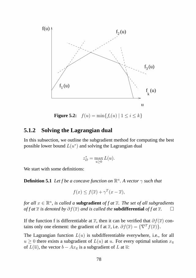
k
f(u)
u
f (u)
f (u)
f (u)
f (u)1
2
3
Figure 5.2: f(u) = min{fi(u) | 1 ≤ i ≤ k}
5.1.2 Solving the Lagrangian dual
In this subsection, we outline the subgradient method for computing the bestpossible lower boundL(u∗) and solving the Lagrangian dual
z∗D = maxu≥0
L(u).
We start with some definitions:
Definition 5.1 Let f be a concave function onRn. A vectorγ such that
f(x) ≤ f(x) + γT (x− x),
for all x ∈ Rn, is called asubgradient of f at x. The set of all subgradientsof f atx is denoted by∂f(x) and is called thesubdifferential of f atx. ¤
If the function f is differentiable atx, then it can be verified that∂f(x) con-tains only one element: the gradient of f atx, i.e. ∂f(x) = {∇T f(x)}.The Lagrangian functionL(u) is subdifferentiable everywhere, i.e., for allu ≥ 0 there exists a subgradient ofL(u) at u. For every optimal solutionxu
of L(u), the vectorb−Axu is a subgradient ofL atu:
78
L(u) = cT xu + uT (b−Axu)
≤ cT xu + uT (b−Axu)
= cT xu + uT (b−Axu) + (b−Axu)T (u− u)
= L(u) + (b−Axu)T (u− u).
Any other subgradient is a convex combination of these subgradients (cf [5]).It is clear thatu∗ is an optimal solution of the Lagrangian dual problem if andonly if 0 ∈ ∂L(u∗).
Remark 5.2 It can be shown that if the Lagrangian problemL(u) can besolved in polynomial time for eachu ≥ 0, then the Lagrangian dual problemcan be solved in polynomial time (see, Schrijver [69], p. 368) ¤
Calculating the exact value may cost too much time, although it might be donein polynomial time. Therefore, one often only approximates the optimal solu-tion of the Lagrangian dual problem. The subgradient method is an algorithmthat is used very often in practice to approximate the value of the Lagrangiandual.
The subgradient optimization algorithm
1. Choose a starting pointu1 ≥ 0 and a sequenceθk; let k = 1.
2. Givenuk, choose a subgradientγk ∈ ∂L(uk). If γk = 0, thenuk isan optimal solution and the algorithm stops. Else defineuk+1 by
uk+1 = ProjU (uk + θkγk).
3. If a stopping criterion is satisfied, then stop. Else setk ← k + 1 andgoto Step 2.
In Step 2, because we want to haveuk+1 ≥ 0, we project the resulting vectoruk+1 onto the set of feasible multipliersU = {u ≥ 0} and obtain
uk+1 = ProjU(uk + θkγk),
79

whereθk is a positive stepsize parameter.
Often a limit on the number of iterations is used as a stopping criterion. Themaximum number of iterations is determined by practical experiments. Theconvergence of the subgradient method depends essentially on the procedureof choosing the step sizesθk. The appropriate choice of the step size is a del-icate problem both in theory and practice. It can be proved that the sequenceof best values generated by the subgradient optimization algorithm
Lk := max {L(ui) : i = 1, ..., k}converges to the maximum value ofL(·), for any stepsize sequenceθk suchthat
limk→∞
θk = 0 and
∞∑
k=0
θk =∞
(see [37]). An example of such a sequence isθk = 1k
. However, this leadsto slow convergence, and other choices for the step sizes, which are moreefficient in practice, often are used. An example is
θk = θ0αk, k = 1,2, ...,
whereα is a scalar satisfying0 < α < 1. A more sophisticated and popularrule is to let
θk =zD −L(uk)
‖γk‖2αk,
whereα satisfies0 < α < 1 andzD is an appropriate estimate of the optimalvaluez∗D.
5.2 Semidefinite Programming
Semidefinite programming (SDP) is an extension of the linear programming(LP). In comparison to standard LP the vectors are replaced by matrix vari-ables and nonnegativity elementwise is replaced by positive semidefiniteness.In addition, LP and SDP are special cases of the conic programming (CP)problem:
80

min < c,x >s.t. Ax = b
x ∈ K,
whereK is a convex cone (K + K ⊆K andαK ⊆K, ∀α ≥ 0), A is a linearoperatorA : Rn → Rm, vectorsc ∈ Rn, b ∈ Rm and<,> is an inner productonRn. LetSn denote the set ofn× n symmetric matrices .
LP is obtained withK = Rn+ (the non-negative orthant) whereas SDP is ob-
tained by lettingK = P (the cone of positive semidefinite matrices). Thecone of positive semidefinite matrices induces a partial order on the setSn,called theLowner partial order
for A,B ∈ Sn A º B if A−B ∈ PThis is the origin of the notationA º 0 for positive semidefinite matrices.
We now discuss in more detail the similarities and differences between LPand SDP.
5.2.1 Geometry
The geometry of polyhedral sets developed for linear programming can beextended to semidefinite programming. This was studied as early as 1948 byBohnenblust [6] and later by Taussky [73] and also Barker and Carlson [2].
Some results similar to LP are: the SDP cone isselfpolar , i.e.
P = P+ := {Y | X • Y ≥ 0, ∀X ∈ P},whereX • Y = Trace XY is the trace inner product. In the spaceRn, bydefinition the trace inner product is the usual inner product, i.e.x • y = xT y.
Also,P ishomogeneous, i.e. for anyX,Y ∈ int(P), there exists an invertiblelinear operatorA that leavesP invariant andA(X) = Y (see [76]).
5.2.2 Duality and Optimality Conditions
Extensions of the optimality conditions and duality theory from linear pro-gramming to semidefinite programming appeared in [4]. However, unlike theLP case, strong duality theorems require a Slater-type constraint qualification.
81

This Slater-type constraint qualification means strict feasibility, i.e., there ex-ists a feasible point in the interior ofP (see Definition 5.2).
Now, consider the typical primal semidefinite program
min C •X(PSDP ) s.t. A(X) = b
X º 0,
whereC ∈ Sn, b ∈ Rm, andA : Sn → Rm, is a linear operator, i.e. thecomponents are defined as
(A(X))i = Ai •X = bi,
for some given symmetric matricesAi.
In order to derive the dual of this program we need the adjoint operator ofA.By definition, it is the operatorAT : Rm → Sn, satisfying
A(X) • y = X •AT (y), ∀X ∈ Sn, ∀y ∈ Rm,
where by definition,A(X) • y =AT (X)y, i.e. in theRm space the trace innerproduct is the usual inner product.
Since,
A(X) • y =m∑
i=1
yi Trace(AiX) = Trace(Xm∑
i=1
yiAi) = X •m∑
i=1
yiAi,
we obtain
AT (y) =m∑
i=1
yiAi.
For constructing the dual we use a Lagrangian approach. The primal equalityconstraints are lifted into the objective by means of a Lagrange multipliery ∈ Rm so that the primal problem readsminXº0 maxy∈Rm C •X + yT (b−A(X)). The dual of the (PSDP) is obtained by interchanging min and max,
minXº0
maxy∈Rm
C •X + yT (b−A(X)) ≥ maxy∈Rm
minXº0
yT b + (C −AT (y)) •X.
82
The construction implies that the right hand side value cannot exceed the valueof the primal problem (see, e.g., Rockafellar [66], Lemma 36.1). For themaximum on the right hand side to be finite, the inner minimization overX º 0 must remain finite for somey ∈ Rm. This requiresC −AT (y) to bepositive semidefinite. We write this condition by introducing a slack matrixZ,
max bT y(DSDP ) s.t. AT y + Z = C
y ∈ Rm, Z º 0.
This is the standard formulation of the dual semidefinite program to (PSDP).
The gap between a dual feasible solution(y,Z) and a primal feasible solutionX is
Trace CX − bT y = Trace(AT y + Z)X −A(X) • y = Trace ZX ≥ 0.
This shows that the duality gap is always nonnegative. The last inequalityfollows from the following well-known lemma:
Lemma 5.1 LetA,B ∈ Sn, A,B º 0. ThenA •B ≥ 0. MoreoverA •B = 0if and only ifAB = 0.
Proof: AB = 0 directly impliesA • B = Trace (AB) = 0. To prove theconverse, consider the transformation ofA,B º 0 to diagonal form
A =n∑
i=1
αiqiqTi , B =
n∑j=1
βjvjvTj ,
whereqi, vj are the orthonormal eigenvectors andαi, βj the correspondingeigenvalues ofA,B. Then withA •B = Trace (AB) we find usingαiβj ≥ 0
A •B =n∑
i,j=1
αiβj(qiqTi vjv
Tj ) =
n∑i,j=1
αiβj(vTj qiq
Ti vj) =
n∑i,j=1
αiβj(qTi vj)
2 ≥ 0
Moreover,A •B = 0 impliesαiβj(qTi vj)
2 = 0 or αiβj(qTi vj) = 0 for all i, j
and then
83
AB =n∑
i,j=1
αiβjqiqTi vjv
Tj =
n∑i,j=1
αiβj(qTi vj)(qiv
Tj ) = 0.
¤
In the following we state that the gap between optimal primal and dual objec-tive value is guaranteed to be zero (i.e. strong duality holds) if at least one of(PSDP) and (DSDP) has a strictly feasible point.
Definition 5.2 A point X is strictly feasible for (PSDP) if it is feasible for(PSDP) and satisfiesX Â 0 (i.e. X is positive definite).A pair (y,Z) is strictly feasible for (DSDP) if it is feasible for (DSDP) andsatisfiesZ Â 0 (i.e. Z is positive definite). ¤
Theorem 5.3 (Strong Duality)Assume that there exists a strictly feasible solution(y, Z) for (DSDP) and let
p∗ = min {C •X | A(X) = b, X º 0} and
d∗ = max {bT y | AT (y) + Z = C, Z º 0}.Thenp∗ = d∗ and ifp∗ is finite it is attained for someX ∈ {X º 0 | A(X) =b}.Proof: See for example [76] or [63]. ¤
The optimality conditions for (PSDP) and (DSDP) are
AT (y) + Z −C = 0 dual feasibilityb−A(X) = 0 primal feasibilityXZ = 0 complementary slacknessX,Z º 0.
X, (y,Z) satisfying these conditions are called a primal-dual optimal pair,Zis the (dual) slack variable. In the case that complementary slackness mayfail, the variables are called a primal-dual feasible pair. Feasible solutionsXandZ satisfying the last equality constraint are calledcomplementary. Thecomplementary slackness constraint can be written in the equivalent formZ •X = 0 (conform Lemma 5.1). The above conditions imply a zero duality gapsince
84

Trace ZX = Trace(C −AT y)X = Trace CX − yT b.
If we perturb the complementary slackness condition,
ZX = µI, µ > 0,
then we get the optimality conditions for a log-barrier problem (see [67]).These are the equations that are used in interior-point methods. However,unlike linear programming there is an interesting subtle complication. Onecannot apply Newton’s method directly, sinceZX is not necessarily symmet-ric (i.e. XZ 6= ZX), and so we end up with an overdetermined system ofequations. There are various ways of modifying this system in order to getgood search directions, see e.g. [53], [74]. Many of these directions work verywell in practice. The algorithms that currently work well are the primal-dualinterior-point algorithms.
5.3 Lagrangian duality for quadratic programs
The material introduced in Sections 5.1 and 5.2 will be used now to applyLagrange duality to quadratic optimization problems. The remaining of thischapter follows closely the paper of Lemarechal and Oustry [48]. In addi-tion at page 93, we have added a comparison of the lower bounds obtainedby linear and complete dualizations with the bounds given by the linear pro-gramming relaxation.
5.3.1 Dualizing a quadratic problem
We start with a well-know lemma, which will be used throughout this chapter:
Lemma 5.2 (Schur’s Lemma)For Q ∈ Sp, P ∈ Sn and ST = (s1, ..., sp) ∈ Rn×p the following two state-ments are equivalent:
i) The matrix
(P ST
S Q
)is positive definite (respectively positive semidefi-
nite).ii) The matricesQ and P − ST Q†S are both positive definite (respectivelypositive semidefinite) andsi ∈ R(Q), for i = 1, ..., p; these last range condi-tions are automatically satisfied whenQ Â 0 (thenR(Q) = Rp).
85

¤
In the above lemma we denoted byQ† the pseudo-inverse of the matrixQ.
Givenm + 1 quadratic functions defined onRn:
qj(x) := xT Qjx + bTj x + cj, j = 0, ...,m, (5.7)
with Qj ∈ Sn, bj ∈ Rn andcj ∈ R, for j = 0, ...,m; we assumec0 = 0. Weconsider the quadratic problem
minx∈Rn
q0(x),
s.t. qj(x) = 0, j = 1, ...,m . (5.8)
Dualizing the costraints (5.8) with Lagrangian multipliersu ∈ Rm yields thefollowing Lagrangian dual function:
L(u) = minx∈Rn
{xT Q(u)x + b(u)T x + c(u)},
whereQ(u) := Q0 +m∑
j=1
ujQj, b(u) := b0 +m∑
j=1
ujbj, c(u) :=m∑
j=1
ujcj = cT u.
The dual problem is to maximizeL. In fact the Lagrangian dual function canbe computed explicitly:
Proposition 5.1 (Lemarechal and Oustry [48])
L(u) =
{c(u)− 1
4b(u)T Q(u)†b(u) if Q(u) º 0 andb(u) ∈ R(Q(u)),
−∞ otherwise.
whereQ† is the pseudo-inverse ofQ andR(Q) is the range (column space)of Q.
Proof: The proof comes directly from the theory regarding the infimum of aquadratic function (see [48]). ¤
86

We want to compute the best lower bound and hence to solve the Lagrangiandualmax
uL(u), which we reformulate as follows (withu ∈ Rm andr ∈ R):
maxu
L(u) = maxu,r
{r | L(u) ≥ r}= max
u,r{r | xT Q(u)x + b(u)T x + c(u) ≥ r, ∀x ∈ Rn}
= maxu,r
{r | (1, xT )
(c(u)− r 1
2b(u)T
12b(u) Q(u)
)(1x
)≥ 0, ∀x ∈ Rn}
= maxu,r
{r |(
c(u)− r 12b(u)T
12b(u) Q(u)
)º 0}.
Therefore the dual problem is equivalent to the following SDP problem withvariablesu ∈ Rm andr ∈ R:
maxu∈Rm,r∈R r
s.t.
(c(u)− r 1
2b(u)T
12b(u) Q(u)
)º 0. (5.9)
Applying duality again to the semidefinite problem (5.9) which is the samewith bidualizing the quadratic problem (5.8). we obtain that the dual of (5.9),i.e., bidual of (5.8) is:
min Q0 •X + bT0 x, X ∈ Sn, x ∈ Rn
(SDP ) s.t. Qj •X + bTj x + cj = 0, j = 1, ...,m(
1 xT
x X
)º 0.
Applying the weak duality theory twice, we see that
val(5.8) ≥ val(5.9) ≤ val(SDP ),
where byval(·) we denote the optimal value of an optimization problem (·).
87
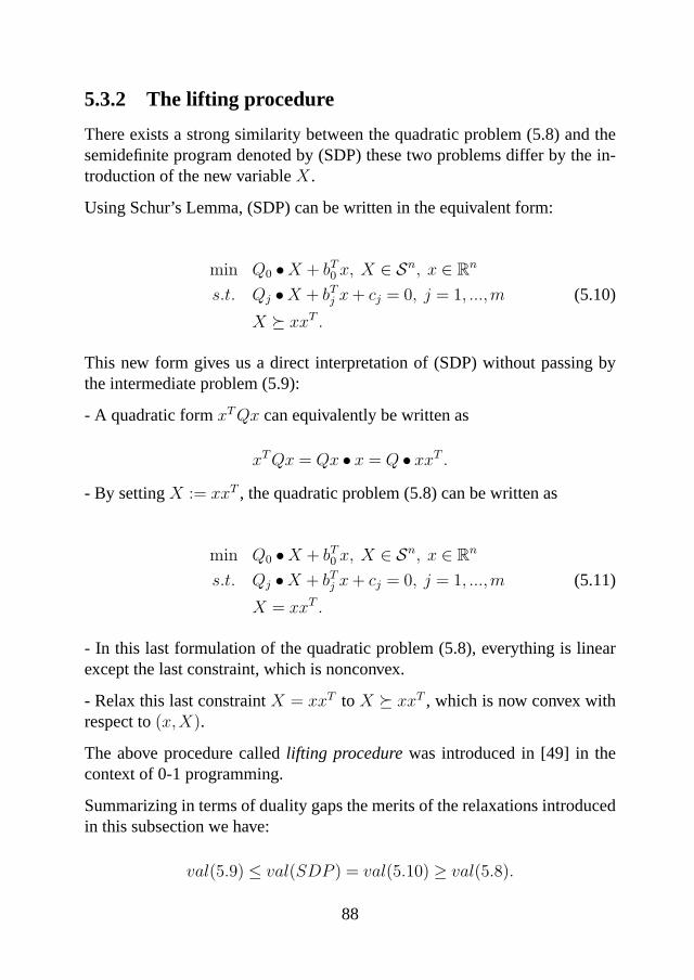
5.3.2 The lifting procedure
There exists a strong similarity between the quadratic problem (5.8) and thesemidefinite program denoted by (SDP) these two problems differ by the in-troduction of the new variableX.
Using Schur’s Lemma, (SDP) can be written in the equivalent form:
min Q0 •X + bT0 x, X ∈ Sn, x ∈ Rn
s.t. Qj •X + bTj x + cj = 0, j = 1, ...,m (5.10)
X º xxT .
This new form gives us a direct interpretation of (SDP) without passing bythe intermediate problem (5.9):
- A quadratic formxT Qx can equivalently be written as
xT Qx = Qx • x = Q • xxT .
- By settingX := xxT , the quadratic problem (5.8) can be written as
min Q0 •X + bT0 x, X ∈ Sn, x ∈ Rn
s.t. Qj •X + bTj x + cj = 0, j = 1, ...,m (5.11)
X = xxT .
- In this last formulation of the quadratic problem (5.8), everything is linearexcept the last constraint, which is nonconvex.
- Relax this last constraintX = xxT to X º xxT , which is now convex withrespect to(x,X).
The above procedure calledlifting procedurewas introduced in [49] in thecontext of 0-1 programming.
Summarizing in terms of duality gaps the merits of the relaxations introducedin this subsection we have:
val(5.9) ≤ val(SDP ) = val(5.10) ≥ val(5.8).
88

The first inequality is weak duality between (5.9) and its dual (SDP). Theequality is Schur’s Lemma. The last inequality holds because the feasibledomain in (5.10) is larger than in (5.8).
It is worth to mentione that the first inequality often holds as an equality (forexample if an appropriate constraint qualification is satisfied).
5.4 Application to 0-1 programming
Consider the following combinatorial optimization problem:
min cT x
s.t. Ax = b (5.12)
x2i − xi = 0, i = 1, ..., n.
In this program the boolean constraintsxi ∈ {0,1}, i = 1, ..., n were mod-elled using the quadratic constraintsx2
i − xi = 0, i = 1, ..., n, and are the onlyquadratic constraints.
Folllowing [48] we present three possible dualizations for the above 0-1 pro-gram and compare the optimal values of the corresponding Lagrangian dualproblems.
5.4.1 Linear dualization
The first possibility is to lift the linear constraints into the objective by meansof a Lagrange multiplieru ∈ Rm. This kind of dualization is called lineardualization. We obtain the following Lagrangian problem:
L1(u) = minx∈{0,1}n
{cT x + uT (Ax− b)}.
This minimization overX = {0,1}n is trivial, the result is a piecewise lineardual function:
L1(u) =n∑
i=1
min {0, (c + AT u)i} − bT u. (5.13)
MaximizingL1 is therefore a nonsmooth optimization problem, which can bedone by a number of methods, see e.g. [37].
89

5.4.2 Complete dualization
Another possible dualization consists in takingX = Rn and in dualizing allthe constraints: the linear as well as the boolean ones. This dualization, whichis called complete dualization, produces another Lagrangian problem, whichnow depends on two dual variables(u, v) ∈ Rm ×Rn:
L2(u, v) = minx∈Rn
{cT x + uT (Ax− b) +n∑
i=1
vi(x2i − xi)}
= minx∈Rn
{(c + AT u− v)T x + xT D(v)x} − bT u.
HereD(v) denotes the diagonal matrix constructed from the vectorv.
Minimizing the above Lagrangian with respect tox (on the wholeRn) can bedone using elementary calculations and we obtain:
L2(u, v) = −bT u +n∑
i=1
Li(u, vi),
where
Li(u, vi) =
−(c + AT u− v)2i
4vi
if vi > 0
0 if vi = 0 and(c + AT u)i = 0−∞ otherwise.
Theorem 5.4 (Lemarechal and Oustry [48])The linear and complete dualizations produce the same duality gap. Moreprecisely:
L1(u) = maxv∈Rn
L2(u, v). (5.14)
¤
Therefore the complete dualization is of moderate interest as compared tolinear dualization: it increases the number of dual variables and produces amore complicated dual function, all this without improving the duality gap.
90
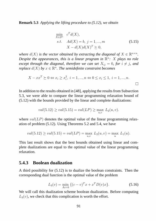
Remark 5.3 Applying the lifting procedure to (5.12), we obtain
minX∈Sn
cT d(X),
s.t. Ad(X) = b, j = 1, ...,m (5.15)
X − d(X)d(X)T º 0,
whered(X) is the vector obtained by extracting the diagonal ofX ∈ Rn×n.Despite the appearances, this is a linear program inRn: X plays no roleexcept through the diagonal, therefore we can setXij = 0, for i 6= j, andreplaced(X) byx ∈ Rn. The semidefinite constraint becomes
X − xxT º 0⇔ xi ≥ x2i , i = 1, ..., n⇔ 0 ≤ xi ≤ 1, i = 1, ..., n.
¤
In addition to the results obtained in [48], applying the results from Subsection5.3, we were able to compare the linear programming relaxation bound of(5.12) with the bounds provided by the linear and complete dualizations:
val(5.12) ≥ val(5.15) = val(LP ) ≥ maxu,v
L2(u, v).
whereval(LP ) denotes the optimal value of the linear programming relax-ation of problem (5.12). Using Theorems 5.2 and 5.4, we have
val(5.12) ≥ val(5.15) = val(LP ) = maxu,v
L2(u, v) = maxu
L1(u).
This last result shows that the best bounds obtained using linear and com-plete dualizations are equal to the optimal value of the linear programmingrelaxation.
5.4.3 Boolean dualization
A third possibility for (5.12) is to dualize the boolean constraints. Then thecorresponding dual function is the optimal value of the problem
L3(v) = minAx=b
{(c− v)T x + xT D(v)x}. (5.16)
We will call this dualization scheme boolean dualization. Before computingL3(v), we check that this complication is worth the effort.
91

Theorem 5.5 (Lemarechal and Oustry [48])There holdsmax
vL3(v) ≥ max
u,vL2(u, v) = max
uL1(u).
Proof: The equality is Theorem 5.3. The inequality is a general result: whenmore constraints are dualized, the duality gap can only increase (see for ex-ample [16]). ¤
We want to computemaxv L3(v). If b /∈R(A) (i.e. Ax = b has no solution inRn) thenval(5.12) = +∞ andmaxv L3(v) = +∞; so there is no duality gap.We therefore assume thatb = Ax for somex ∈ Rn. Assumem′ = rank(A)(i.e. the rank of A), letZ be a matrix withn−m′ columns that form a basisof N (A), whereN (A) denote the null space of A. Thus
Ax = b with x ∈ Rn ⇐⇒ x = x + Zy with y ∈ Rn−m′,
so that (5.12) is equivalent to the following problem iny
min cT Zy + cT x,
s.t. yT ZTi Ziy + (2xT
i − 1)Ziy + x2i − xi = 0, i = 1, ..., n . (5.17)
HereZi ∈ Rn−m′denotes theith row ofZ.
Theorem 5.6 (Lemarechal and Oustry [48])The dual valuemaxv L3(v), associated with (5.12), (5.16), is the value of theSDP problem
max r
s.t.
(c(v)− r 1
2b(v)T
12b(v) Q(v)
)º 0, (5.18)
where
c(v) := xT D(v)x + (c− v)T x,
b(v) := 2D(v)x + c− v,Q(v) := ZD(v)ZT .
¤
92

5.4.4 Inequality constraints
Suppose that the general optimization problem (5.12) contains inequality con-straints; say
min cT x
s.t. Ax ≤ b (5.19)
xi ∈ {0,1} i = 1, ..., n
or even a mixture of equalities and inequalities.
The new formulation of the general optimization problem (5.19) does notaffect the linear dualization. The only change is that the dual problem nowhas positivity constraints and becomesmaxu≥0 L1(u); but the duality gap stillcorresponds to replacing{0,1} by [0,1].
Remark 5.4 Due to the general result: the more constraints are dualized,the weaker the bound becomes, one possibility to obtain a better lower boundthan the bound provided by the linear dualization is to dualize just some of thelinear constraints. One would dualize only the constraints that are difficult todeal with directly. ¤
The complete dualization is also unaffected. Theu-part of the dual variablesis again constrained toRm
+ , and we again obtain a scheme equivalent to lineardualization:
Theorem 5.7 (Lemarechal and Oustry [48])For (5.20), linear and complete dualizations produce the same duality gap.
¤
By contrast, the boolean dualization breaks down: the dual fuction becomes
minAx≤b
{(c− v)T x + xT D(v)x}.
SinceD(v) has no reason to be positive semidefinite, the above problem is adifficult nonconvex problem.
Therefore the boolean dualization can treat only equality constraints; as forthe inequalities, they have to be treated by a linear strategy.
93

5.5 Concluding remarks
We presented three possible dualizations of 0-1 programming problem (con-taining only equality constraints): linear, complete and boolean dualizationsand we compared the bounds obtained using these dualizations with the boundprovided by the linear programming relaxation.
We showed that the bounds obtained by linear and complete dualizations areequal to the optimal value of the linear programming relaxation of the initial0-1 program. In addition the bounds obtained by using boolean dualizationmay be better.
The results obtained for linear and complete dualizations hold also in the casewhen the initial 0-1 program contains inequality constraints, but break downin the case of boolean dualization. Therefore the boolean dualization can treatonly equality constraints; as for the inequalities, they have to be treated by alinear strategy.
94

Chapter 6
Solving the GMST problem withLagrangian Relaxation
As we have seen in the previous chapter, we may obtain better lower boundsthan the bound provided by linear and complete dualizations if we dualizeonly the ”nasty” linear constraints, i.e. the constraints that are difficult to dealwith directly.
In this chapter we present an algorithm to obtain ”good” lower bounds (bet-ter than the bounds provided by the LP relaxation) for the GMST problem.The algorithm is based on a Lagrangian relaxation of a bidirectional multi-commodity flow formulation of the problem. The subgradient optimizationalgorithm is used to obtain lower bounds. Computational results are reportedfor many instances of the problem.
95
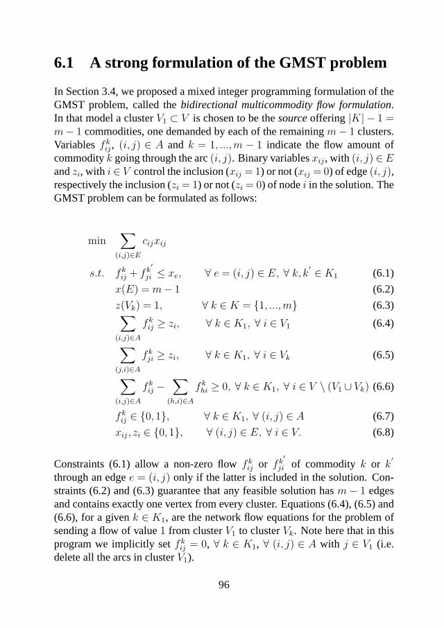
6.1 A strong formulation of the GMST problem
In Section 3.4, we proposed a mixed integer programming formulation of theGMST problem, called thebidirectional multicommodity flow formulation.In that model a clusterV1 ⊂ V is chosen to be thesourceoffering |K| − 1 =m− 1 commodities, one demanded by each of the remainingm− 1 clusters.Variablesfk
ij, (i, j) ∈ A and k = 1, ...,m − 1 indicate the flow amount ofcommodityk going through the arc(i, j). Binary variablesxij, with (i, j) ∈Eandzi, with i ∈ V control the inclusion (xij = 1) or not (xij = 0) of edge(i, j),respectively the inclusion (zi = 1) or not (zi = 0) of nodei in the solution. TheGMST problem can be formulated as follows:
min∑
(i,j)∈E
cijxij
s.t. fkij + fk
′
ji ≤ xe, ∀ e = (i, j) ∈ E, ∀ k, k′ ∈K1 (6.1)
x(E) = m− 1 (6.2)
z(Vk) = 1, ∀ k ∈ K = {1, ...,m} (6.3)∑
(i,j)∈A
fkij ≥ zi, ∀ k ∈ K1, ∀ i ∈ V1 (6.4)
∑
(j,i)∈A
fkji ≥ zi, ∀ k ∈ K1, ∀ i ∈ Vk (6.5)
∑
(i,j)∈A
fkij −
∑
(h,i)∈A
fkhi ≥ 0, ∀ k ∈K1, ∀ i ∈ V \ (V1 ∪ Vk) (6.6)
fkij ∈ {0,1}, ∀ k ∈ K1, ∀ (i, j) ∈ A (6.7)
xij, zi ∈ {0,1}, ∀ (i, j) ∈ E, ∀ i ∈ V. (6.8)
Constraints (6.1) allow a non-zero flowfkij or fk
′ji of commodity k or k
′
through an edgee = (i, j) only if the latter is included in the solution. Con-straints (6.2) and (6.3) guarantee that any feasible solution hasm− 1 edgesand contains exactly one vertex from every cluster. Equations (6.4), (6.5) and(6.6), for a givenk ∈ K1, are the network flow equations for the problem ofsending a flow of value1 from clusterV1 to clusterVk. Note here that in thisprogram we implicitly setfk
ij = 0, ∀ k ∈ K1, ∀ (i, j) ∈ A with j ∈ V1 (i.e.delete all the arcs in clusterV1).
96

6.2 Defining a Lagrangian problem
We relax equations (6.4), (6.5) and (6.6) in a Lagrangian fashion. Lettik (≥ 0,∀ i /∈ V1 ∪ Vk, ∀ k ∈ K1) be the Lagrange multipliers corresponding to (6.6),t(1)ik (≥ 0, ∀ i ∈ V1, ∀ k ∈ K1) be the Lagrange multipliers corresponding
to (6.4) and lett(k)ik (≥ 0, ∀ i ∈ Vk, ∀ k ∈ K1) be the Lagrange multipliers
corresponding to (6.5).
Then the coefficientCkij of fk
ij in the objective function of the Lagrangian dualprogram is given by
Ckij =
−t(1)ik − t
(k)jk if i ∈ V1 andj ∈ Vk
−tik − t(k)jk if i /∈ V1 ∪ Vk andj ∈ Vk
−t(1)ik + tjk if i ∈ V1 andj /∈ V1 ∪ Vk
−tik + tjk if i /∈ V1 ∪ Vk andj /∈ V1 ∪ Vk
0 otherwise,
the coefficient ofzi, pi is given by
pi =
m∑
k=2
t(1)ik if i ∈ V1
m∑
k=2
t(k)ik if i ∈ Vk,
and the Lagrangian dual program is:
min∑
(i,j)∈E
cijxij +∑
(i,j)∈A
∑
k∈K1
Ckijf
kij +
∑i∈V
pizi
s.t. fkij + fk
′
ji ≤ xe, ∀ e = (i, j) ∈ E, ∀ k, k′ ∈K1
x(E) = m− 1
z(Vk) = 1, ∀ k ∈ K = {1, ...,m}fk
ij ∈ {0,1}, ∀ k ∈ K1, ∀ (i, j) ∈ A
xij, zi ∈ {0,1}, ∀ (i, j) ∈ E, ∀ i ∈ V.
From constraint (6.1), it is simple to deduce that the best contribution to thedual objective function is given by:
97
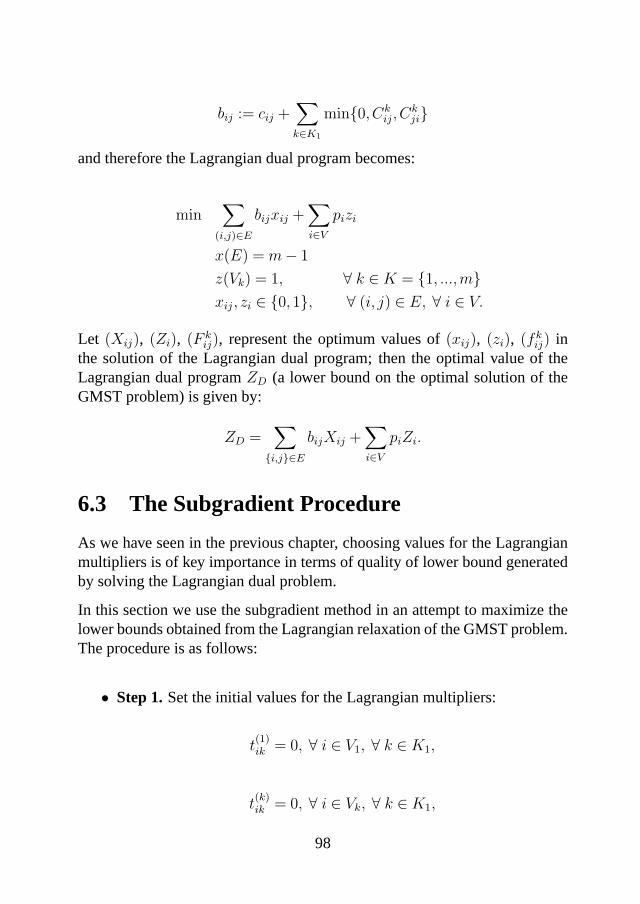
bij := cij +∑
k∈K1
min{0,Ckij,C
kji}
and therefore the Lagrangian dual program becomes:
min∑
(i,j)∈E
bijxij +∑i∈V
pizi
x(E) = m− 1
z(Vk) = 1, ∀ k ∈K = {1, ...,m}xij, zi ∈ {0,1}, ∀ (i, j) ∈ E, ∀ i ∈ V.
Let (Xij), (Zi), (F kij), represent the optimum values of(xij), (zi), (fk
ij) inthe solution of the Lagrangian dual program; then the optimal value of theLagrangian dual programZD (a lower bound on the optimal solution of theGMST problem) is given by:
ZD =∑
{i,j}∈E
bijXij +∑i∈V
piZi.
6.3 The Subgradient Procedure
As we have seen in the previous chapter, choosing values for the Lagrangianmultipliers is of key importance in terms of quality of lower bound generatedby solving the Lagrangian dual problem.
In this section we use the subgradient method in an attempt to maximize thelower bounds obtained from the Lagrangian relaxation of the GMST problem.The procedure is as follows:
• Step 1.Set the initial values for the Lagrangian multipliers:
t(1)ik = 0, ∀ i ∈ V1, ∀ k ∈ K1,
t(k)ik = 0, ∀ i ∈ Vk, ∀ k ∈ K1,
98
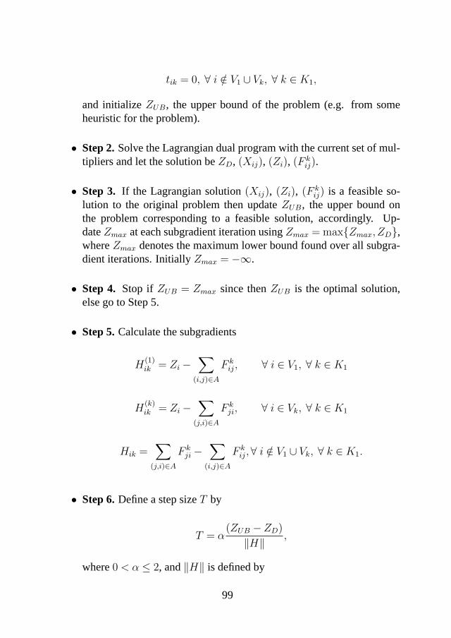
tik = 0, ∀ i /∈ V1 ∪ Vk, ∀ k ∈K1,
and initializeZUB, the upper bound of the problem (e.g. from someheuristic for the problem).
• Step 2.Solve the Lagrangian dual program with the current set of mul-tipliers and let the solution beZD, (Xij), (Zi), (F k
ij).
• Step 3. If the Lagrangian solution(Xij), (Zi), (F kij) is a feasible so-
lution to the original problem then updateZUB, the upper bound onthe problem corresponding to a feasible solution, accordingly. Up-dateZmax at each subgradient iteration usingZmax = max{Zmax,ZD},whereZmax denotes the maximum lower bound found over all subgra-dient iterations. InitiallyZmax = −∞.
• Step 4. Stop if ZUB = Zmax since thenZUB is the optimal solution,else go to Step 5.
• Step 5.Calculate the subgradients
H(1)ik = Zi −
∑
(i,j)∈A
F kij, ∀ i ∈ V1, ∀ k ∈ K1
H(k)ik = Zi −
∑
(j,i)∈A
F kji, ∀ i ∈ Vk, ∀ k ∈ K1
Hik =∑
(j,i)∈A
F kji −
∑
(i,j)∈A
F kij,∀ i /∈ V1 ∪ Vk, ∀ k ∈ K1.
• Step 6.Define a step sizeT by
T = α(ZUB −ZD)
‖H‖ ,
where0 < α ≤ 2, and‖H‖ is defined by
99
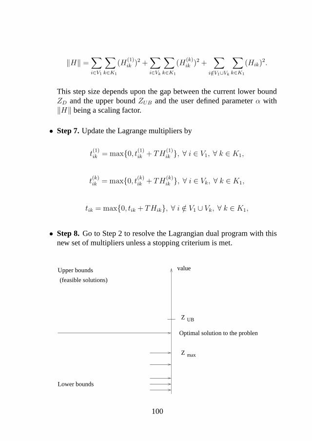
‖H‖ =∑i∈V1
∑
k∈K1
(H(1)ik )2 +
∑i∈Vk
∑
k∈K1
(H(k)ik )2 +
∑
i/∈V1∪Vk
∑
k∈K1
(Hik)2.
This step size depends upon the gap between the current lower boundZD and the upper boundZUB and the user defined parameterα with‖H‖ being a scaling factor.
• Step 7.Update the Lagrange multipliers by
t(1)ik = max{0, t(1)
ik + TH(1)ik }, ∀ i ∈ V1, ∀ k ∈ K1,
t(k)ik = max{0, t(k)
ik + TH(k)ik }, ∀ i ∈ Vk, ∀ k ∈K1,
tik = max{0, tik + THik}, ∀ i /∈ V1 ∪ Vk, ∀ k ∈K1,
• Step 8.Go to Step 2 to resolve the Lagrangian dual program with thisnew set of multipliers unless a stopping criterium is met.
Optimal solution to the problem
value
Z
Upper bounds
(feasible solutions)
Lower bounds
Z max
UB
100

Figure 6.1: Subgradient optimization
Figure 6.1 illustrates the situation during the subgradient iterations. As shownin this figure, we plot the lower bound found at each subgradient iteration onthe value line. The best (maximum) of these lower bounds isZmax.
Initially we setα = 2. If Zmax is not improved (i.e. increased) in the lastNsubgradient iterations with the current value ofα then we halveα. Based onexperimenting (computationally) with different values ofN , it seems to bereasonable to choose the valueN = 30.
In our experiments we setZUB = ZOPT , whereZOPT is the optimal value ofthe GMST problem calculated using the rooting procedure (see Section 3.6).
6.4 Computational Results
We used the same classes of instances as in Subsection 3.6. According to themethod of generating the edge costs, the problems generated are classifiedinto three types:
• structured Euclidean case
• unstructured Euclidean case
• non-Euclidean case.
For the instances in the structured Euclidean casem squares (clusters) are”packed in a square” and in each of thesem clustersnc nodes are selectedrandomly. The costs between nodes are the Euclidean distances between thenodes. So in this model the clusters can be interpreted as physical clusters. Inthe other models such an interpretation is not valid.
For the unstructured Euclidean casen = mnc nodes are generated randomly in[0,100]2 with costs given by the Euclidean distances. But then the clusters arechoosen randomly among these points. Finally in the non-Euclidean modelthe edge costs are randomly generated on[0,100].
Our computational experiments were performed on a HP 9000/735 computerwith a 125 Mhz processor and 144 Mb memory. Our Lagrangian relaxationscheme is written in C and compiled with a HP-UX cc compiler.
101
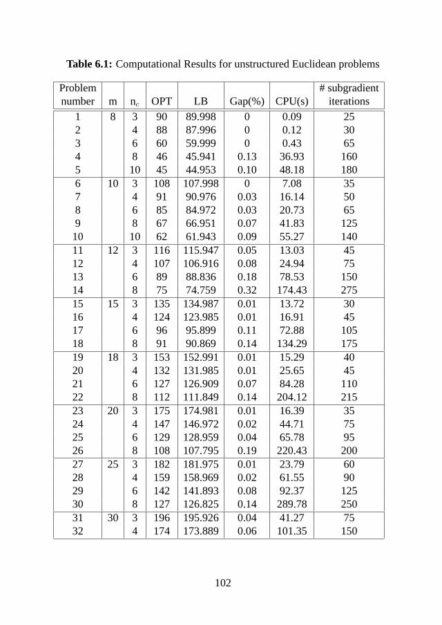
Table 6.1: Computational Results for unstructured Euclidean problems
Problem # subgradientnumber m nc OPT LB Gap(%) CPU(s) iterations
1 8 3 90 89.998 0 0.09 252 4 88 87.996 0 0.12 303 6 60 59.999 0 0.43 654 8 46 45.941 0.13 36.93 1605 10 45 44.953 0.10 48.18 1806 10 3 108 107.998 0 7.08 357 4 91 90.976 0.03 16.14 508 6 85 84.972 0.03 20.73 659 8 67 66.951 0.07 41.83 12510 10 62 61.943 0.09 55.27 14011 12 3 116 115.947 0.05 13.03 4512 4 107 106.916 0.08 24.94 7513 6 89 88.836 0.18 78.53 15014 8 75 74.759 0.32 174.43 27515 15 3 135 134.987 0.01 13.72 3016 4 124 123.985 0.01 16.91 4517 6 96 95.899 0.11 72.88 10518 8 91 90.869 0.14 134.29 17519 18 3 153 152.991 0.01 15.29 4020 4 132 131.985 0.01 25.65 4521 6 127 126.909 0.07 84.28 11022 8 112 111.849 0.14 204.12 21523 20 3 175 174.981 0.01 16.39 3524 4 147 146.972 0.02 44.71 7525 6 129 128.959 0.04 65.78 9526 8 108 107.795 0.19 220.43 20027 25 3 182 181.975 0.01 23.79 6028 4 159 158.969 0.02 61.55 9029 6 142 141.893 0.08 92.37 12530 8 127 126.825 0.14 289.78 25031 30 3 196 195.926 0.04 41.27 7532 4 174 173.889 0.06 101.35 150
102

Table 6.2: Computational Results for structured Euclidean problems
Problem # subgrad.number m nc OPT LB Gap(%) CPU(s) iterations
1 8 3 983 982.998 0 0.08 252 4 966 965.993 0 0.18 303 6 960 959.988 0 0.49 654 8 934 933.953 0.01 36.91 1605 10 922 921.949 0.01 48.72 1806 10 3 1251 1250.998 0 7.23 357 4 1243 1242.980 0 16.59 508 6 1240 1239.975 0 20.93 659 8 1225 1224.956 0 41.98 12510 10 1208 61.943 0 55.31 14011 12 3 1616 1615.951 0 14.63 4512 4 1545 1544.908 0.01 25.76 7513 6 1487 1486.841 0.01 78.96 15014 8 1458 1457.745 0.02 174.81 27515 15 3 1977 1976.985 0 14.79 3016 4 1966 1965.981 0 18.85 4517 6 1946 1945.909 0 75.81 10518 8 1932 1931.899 0.01 138.77 17519 18 3 2384 2383.992 0 17.16 4020 4 2365 2364.985 0 27.70 4521 6 2352 2351.904 0 89.22 11022 8 2338 2337.863 0.01 225.08 21523 20 3 2765 2764.972 0 17.32 3524 4 2741 2740.968 0 46.81 7525 6 2728 2727.956 0 69.77 9526 8 2709 2708.797 0.01 231.48 20027 25 3 3112 3111.967 0 24.72 6028 4 3094 3093.958 0 64.51 9029 6 3075 3074.795 0.01 97.38 12530 8 3058 3057.715 0.01 298.89 25031 30 3 3478 3477.832 0 52.13 7532 4 3452 3451.787 0.01 138.96 150
103
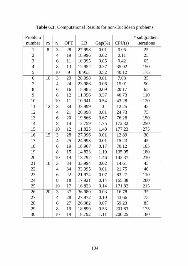
Table 6.3: Computational Results for non-Euclidean problems
Problem # subgradientnumber m nc OPT LB Gap(%) CPU(s) iterations
1 8 3 28 27.998 0.01 0.05 252 4 19 18.996 0.02 0.11 253 6 11 10.995 0.05 0.42 654 8 13 12.952 0.37 35.02 1505 10 9 8.953 0.52 40.12 1756 10 3 29 28.998 0.01 7.03 357 4 24 23.986 0.06 15.01 508 6 16 15.985 0.09 20.17 659 8 12 11.956 0.37 40.73 11010 10 11 10.941 0.54 43.28 12011 12 3 34 33.999 0 12.25 4512 4 21 20.998 0.01 24.73 7513 6 20 19.866 0.67 76.28 15014 8 14 13.759 1.75 172.32 25015 10 12 11.825 1.48 177.23 27516 15 3 28 27.996 0.01 12.89 3017 4 25 24.993 0.01 15.23 4518 6 19 18.967 0.17 70.12 10519 8 15 14.823 1.19 135.95 18020 10 14 13.792 1.46 142.37 21021 18 3 34 33.994 0.02 14.61 4522 4 34 33.995 0.01 21.75 4023 6 22 21.974 0.07 83.27 11024 8 18 17.921 0.14 165.38 20025 10 17 16.823 0.14 171.82 21526 20 3 37 36.989 0.03 16.78 3527 4 28 27.972 0.10 43.66 7528 6 27 26.982 0.07 59.23 8529 8 19 18.899 0.53 201.83 17530 10 19 18.792 1.11 200.25 180
104
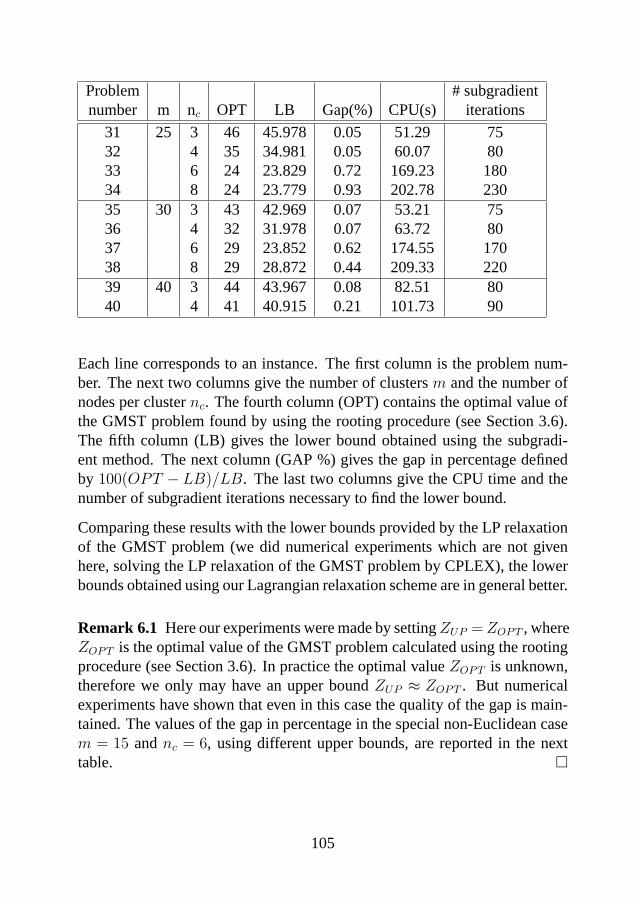
Problem # subgradientnumber m nc OPT LB Gap(%) CPU(s) iterations
31 25 3 46 45.978 0.05 51.29 7532 4 35 34.981 0.05 60.07 8033 6 24 23.829 0.72 169.23 18034 8 24 23.779 0.93 202.78 23035 30 3 43 42.969 0.07 53.21 7536 4 32 31.978 0.07 63.72 8037 6 29 23.852 0.62 174.55 17038 8 29 28.872 0.44 209.33 22039 40 3 44 43.967 0.08 82.51 8040 4 41 40.915 0.21 101.73 90
Each line corresponds to an instance. The first column is the problem num-ber. The next two columns give the number of clustersm and the number ofnodes per clusternc. The fourth column (OPT) contains the optimal value ofthe GMST problem found by using the rooting procedure (see Section 3.6).The fifth column (LB) gives the lower bound obtained using the subgradi-ent method. The next column (GAP %) gives the gap in percentage definedby 100(OPT − LB)/LB. The last two columns give the CPU time and thenumber of subgradient iterations necessary to find the lower bound.
Comparing these results with the lower bounds provided by the LP relaxationof the GMST problem (we did numerical experiments which are not givenhere, solving the LP relaxation of the GMST problem by CPLEX), the lowerbounds obtained using our Lagrangian relaxation scheme are in general better.
Remark 6.1 Here our experiments were made by settingZUP = ZOPT , whereZOPT is the optimal value of the GMST problem calculated using the rootingprocedure (see Section 3.6). In practice the optimal valueZOPT is unknown,therefore we only may have an upper boundZUP ≈ ZOPT . But numericalexperiments have shown that even in this case the quality of the gap is main-tained. The values of the gap in percentage in the special non-Euclidean casem = 15 andnc = 6, using different upper bounds, are reported in the nexttable. ¤
105

m nc OPT UB Gap(%) CPU(s) # subgrad. iterations
15 6 19 - 0.17 70.12 10515 6 - 19.5 0.19 70.33 10515 6 - 20 0.20 70.67 10515 6 - 21 0.23 71.09 105
The first two columns give the number of clustersm and the number of nodesper clusternc. The third column (OPT) contains the optimal value of theGMST problem found by using the rooting procedure (see Section 3.6). Theforth column (UB) gives the upper bound. The next column (GAP %) givesthe gap in percentage defined by100(UB −LB)/LB. The last two columnsgive the CPU time and the number of subgradient iterations.
6.5 Concluding remarks
We presented a Lagrangian relaxation of a bidirectional multicommodity flowformulation of the GMST problem. The subgradient optimization algorithmwas used to obtain lower bounds.
Computational experiments (by settingZUP = ZOPT ) show that using ourLagrangian relaxation scheme are in general better than the lower boundsprovided by the linear programming relaxation of the GMST problem. Thisresult holds even in the case when we may have available an upper boundZUP ≈ ZOPT .
106

Chapter 7
Heuristic Algorithms
The techniques described in this chapter are the ones which are known bythe term heuristics, i.e. techniques which seek near-optimal solutions at areasonable computational cost without being able to guarantee optimality, oreven in many cases to state how close to optimality a particular solution is.
In the first sections we present some basic theory of heuristic algorithms andlocal search. In Section 7.4 we present the Simulated Annealing algorithm.Finally, in the last section we solve the GMST problem with Simulated An-nealing.
107

7.1 Introduction
We have mentioned that many combinatorial optimization problems areNP-hard [21], and the theory ofNP-completeness has reduced hopes thatNP-hardproblems can be solved within polynomially bounded computation times.Nevertheless, sub-optimal solutions are sometimes easy to find. Consequently,there is much interest in approximation and heuristic algorithms that can findnear optimal solutions within reasonable running time.
In mathematical programming, aheuristic methodor heuristic for short is aprocedure that determines good or near-optimal solutions to an optimizationproblem. As opposed to exact methods, heuristics carry no guarantee that anoptimal solution will be found.
Practically, for many realistic optimization problems good solutions can befound efficiently, and heuristics are typically among the best strategies interms of efficiency and solution quality for problems of realistic size and com-plexity. Heuristics can be classified as eitherconstructive(greedy) or aslocalsearchheuristics. The former are typically one-pass algorithms whereas thelatter are strategies ofiterative improvement. We will be concerned exclu-sively with local search heuristics here.
Useful references on heuristic methods can be found in Osman and Laporte[56] and Reeves [64].
7.2 Local and global optima
The following concepts are taken from [57].
Definition 7.1 An instance of an optimization problem is a pair (S, c),whereS is any set, the domain of feasible points;c is the cost function
c : S → R
The problem is to find ans ∈ S for which
c(s) ≤ c(y) for all y ∈ S.
Such a point is calledglobally optimal solution to the given instance or,when no confusion can rise, simply anoptimal solution. ¤
108

Given a feasible points ∈ S in a particular problem, it is useful in manysituations to define a setN(s) of points that are ”close” in some sense to thepoints.
Definition 7.2 Given an optimization problem with instances(S, c), a neigh-bourhood is a mapping
N : S → 2S
defined for each instance. ¤
In many combinatorial problems, there are quite natural choices forN sug-gested by the structure ofS. It is often possible to find a solutions which isbest in the sense that there is nothing better in its neighbourhoodN(S).
Definition 7.3 Given an instance(S, c) of an optimization problem a neigh-bourhoodN , a feasible solutions ∈ S is calledlocally optimal with respectto N if
c(s) ≤ c(g) for all g ∈ N(s).
¤
7.3 Local Search
In the next two sections we present the basic theory of local search and simu-lated annealing. We follow the description of Reeves [64].
Local search (LS) is a term for the extremely simple concept underlying manymodern heuristic techniques, such as Simulated Annealing, Tabu Search andGenetic Algorithms.
Suppose that we have a minimization problem over a set of feasible solutionsS and a cost functionc : S → R. The optimal solution could be obtained bycalculatingc(s) for eachs ∈ S and selecting the minimum. This method isimpracticable when the setS is big which is the case of the most real-lifeproblems. Local search overcomes this difficulty by searching only a smallsubset of the solution space. This is achieved by defining a neighbourhoodstructure on the solution space and searching the neighbourhood of the cur-rent solution for an improvement. If there is no neighbour which results in an
109

improvement to the cost function, the current solution is taken as an approx-imation to the optimum. If an improvement is found, the current solution isreplaced by the improvement and the process is repeated.
Therefore the local search process can be described as follows:
Local search for a problem with solution spaceS, cost functioncand neighbourhood structureN
1. Select a starting solutions0 ∈ S;
2. RepeatSelects such thatc(s) < c(s0) by a suitable method;Replaces0 by s;
Until c(s) > c(s0) for all s ∈ N(s0).
s0 is the approximation of the optimal solution.
A central problem for local search is the occurence oflocal optima, i.e. nodesin the search space where no neighbour strictly improves over the current nodein terms of the cost function, but which are not global optima. Many strate-gies have been proposed that address the problem of how to overcome thelocal optima. In many cases, non-improving local moves are admitted basedon a probabilistic decision or based on the history of the search. To obtainguiding principles for designing effective optimization strategies, a numberof conceptual meta-level strategies have been employed with local search.These strategies are referred to asmetaheuristic, a term introduced by Glover[25].
In contrast to individual heuristic algorithms that are designed to solve a spe-cific problem, metaheuristics are strategic problem solving frameworks thatcan be adapted to solve a wide variety of problems. A metaheuristic frame-work includes a set of problem-solving principles that are sometimes basedon natural or physical processes, and a set of control parameters. Applica-tion of a metaheuristic stategy to a specific problem involves choosing, andsometimes fine-tuning, these parameters.
Metaheuristic methods are not normally expected to outperform specializedheuristics on a problem. Their main purpose is to deal with difficult problems
110

for which no specialized algorithm is known. However, some studies havedemonstrated that certain metaheuristics perform as well or better than specialheuristics for some well-known difficult problems such as traveling salesman,graph partitioning and facility layout problems.
The most important metaheuristics for optimization are given in the follow-ing:
Simulated Annealing, introduced for optimization by Kirkpatricket al. [44]in 1983. The central idea is to accept a candidate move that increases the so-lution quality based on a probabilistic decision. During the time of the search,the probability of acceptance of deteriorating moves is decreased accordingto a givenannealing schedule.
Genetic Algorithmswere invented by Holland and model optimization as anevolutionary process. The strategy is to have a pool of ”chromosomes” anditeratively apply the principles of mutation, mating and selection to attain”survival of the fittest” [39]. Genetic algorithms extend the basic local searchscheme to populations of solutions.
Tabu Searchwas first suggested by Glover [25] and uses information based onthe history of the search [26]. It has been succesfully applied to obtain optimalor sub-optimal solutions for many combinatorial optimization problems suchas scheduling, time-tabling, travelling salesman, etc.. The central idea is theuse of adaptive memory to overcome local optima by driving the search todifferent parts of the search space (diversification) or back to promising parts(intensification).
Artificial Neural Networksmake use of the metaphor of the neuron and areorganized in network structures. The network of nodes is iteratively modi-fied by adjusting the interconnections between neurons according to variousschemes [77].
For particular application problems, the metaheuristics require concrete im-plementation and their success varies for different application domains.
111

7.4 Simulated Annealing
7.4.1 Introduction
The ideas that form the basis of simulated annealing were first published byMetropoliset al. [52] in 1953 as an algorithm to simulate the cooling of ma-terial in a heat bath, a process known as annealing. If solid material is heatedpast its melting point and then cooled back into a solid state, the structuralproperties of the cooled solid depend on the rate of cooling. The annealingprocess can be simulated by regarding the material as a system of particles.Essentially, Metropolis’ algorithm simulates the change in energy of the sys-tem during the cooling process, as it converges to a steady ’frozen’ state.Kirkpatrick et al. [44] and Cerny [9] suggested that this type of simulationcould be used to search the feasible solutions of an optimization problem.Their approach can be regarded as a variant of the local search technique.
In the case of a minimization problem the local search employ a descent strat-egy, in which the search always moves in a direction of improvement. How-ever, such a strategy often results in convergence to a local rather than a globaloptimum.
In order to overcome the local optima, in the simulated annealing heuristicnon-improving local moves are allowed, but their frequency is governed by aprobability function which changes as the algorithm progresses.
The inspiration for this form of control was Metropolis’ work in statisticalthermodynamics. The laws of thermodynamics state that at temperatureT ,the probability of an increase in energy of magnitudeδE is given by
p(δE) = exp(−δE/kT ) (7.1)
wherek is a physical constant known as Boltzmann’s constant.
Metropolis’ simulation generates a perturbation and calculates the resultingenergy change. If energy has decreased the system moves to this new state.If energy has increased, the new state is accepted according to the probabilitygiven in Equation 7.1. The process is repeated for a predetermined number ofiterations at each temperature, after which the temperature is decreased untilthe system freezes into a steady state.
Kirkpatrick et al. [44] and Cerny [9] independently showed that Metropolis’algorithm could be applied to optimization problems by mapping the elements
112

of the physical cooling process onto the elements of a combinatorial optimiza-tion problem as shown in the following table:
Thermodynamic simulation Combinatorial optimizationSystem states Feasible solutions
Energy CostChange of state Change of solution
Temperature Control parameterFrozen state Heuristic solution
Therefore any local search algorithm can be converted into an annealing al-gorithm by sampling the neighbourhoods randomly and allowing the accep-tance of an inferior solution with respect to cost minimization according to theprobability given in Equation 7.1. The level of acceptance then depends onthe magnitude of the increase in the cost function and the current temperature.
7.4.2 The annealing algorithm
As we have seen the main disadvantage of local search is its likelihood offinding a local, rather than global, optimum. By allowing some non-imrovinglocal moves in a controlled manner, simulated annealing overcomes this prob-lem. The annealing algorithm can be stated as follows:
Simulated annealing for a minimization problem with solution spaceS,objective function c and neighbourhood structureN
113

Select a starting solutions0 ∈ S, an initial temperatureT0 > 0 and atemperature reduction functionα;
RepeatRepeat
Randomly selects ∈ N(s0) and computeδ = c(s)− c(s0);If δ < 0thens0 = selse generate randomp uniformly in the range(0,1);if p < exp(−δ/T ) thens0 = s
Until iterationcount = L;SetT = α(T );Until stopping condition is true.
s0 is the approximation of the optimal solution.
HereL represents the number of repetitions at each temperature, i.e. the num-ber of randomly chosen candidate solutions in the neighborhood of the currentsolution that are evaluated.
At each stage,L randomly chosen candidate solutions in the neighborhoodof the current solution are evaluated. If a candidate solution improves onthe current solution, it is accepted. Otherwise, it is accepted with a proba-bility p(T, δ) = exp(−δ/T ), which depends on the control parameterT (thetemperature in the physical equivalent) and the amountδ by which a moveworsens the current solution. This relation ensures that the probability of ac-cepting a move to a very poor solution is very small. At the completitionof each stage, the temperatureT is reduced at cooling rater. Given a rel-atively high temperatureT at the beginning of the process, the probabilityof accepting non-improving moves is fairly high. As the process continues,the temperature decreases and non-improving moves become less likely. Thesearch is continued until there is some evidence to suggest that there is a verylow probability of improving on the best solution found so far. At this stage,the system is said to be frozen.
The algorithm given is very general, and a number of decisions must be madein order to implement it for the solution of a particular problem. These can bedivided into two categories:
114
• generic decisions which are concerned with parameters of the annealingalgorithm itself. These include factors such as the initial temperature,the cooling schedule (governed by the parameterL, i.e. number ofrepetitions and the choice of the temperature reduction functionα) andthe stopping condition.
• problem specific decisions and involves the choice of the space of feasi-ble solutions, the form of the cost function and the neighborhood struc-ture employed.
Simulated annealing has the advantage that it is simple in concept and im-plementation. The procedure improves on descent methods by reducing theprobability of getting stuck at a poor but locally optimal solution. Simulatedannealing has been applied successfully to many hard optimization problems;see e.g., the bibliography by Osman and Laporte [56].
Since Kirkpatrick’s original paper there has been much research into the the-oretical convergence of the annealing algorithm. The theoretical results arebased on the fact that the behavior of the simulated annealing algorithm canbe modelled using Markov chains (see e.g. [5]).
7.5 Solving the GMST problem with SimulatedAnnealing
7.5.1 The local-global formulation of the GMST problem
In order to solve the GMST problem with simulated annealing we use thelocal-global formulation of the problem (see Section 3.5), which arises fromdistinguishing betweenglobal, i.e., inter-cluster connections, andlocal ones.We introduced the variablesyij (i, j ∈ {1, ...,m}) to describe the global con-nections:yij = 1 if clusterVi is connected to clusterVj andyij = 0 otherwiseand we assumed thaty represents a spanning tree. The convex hull of all thesey-vectors is generally known as the spanning tree polytope on the contractedgraph with vertex set{V1, ..., Vm} (which we assume to be complete) and canbe represented by the following constraints:
115

∑
{i,j}yij = m− 1
yij = λkij + λkji, for 1 ≤ k, i, j ≤m andi 6= j∑j
λkij = 1, for 1 ≤ k, i, j ≤m andi 6= k
λkkj = 0, for 1 ≤ k, j ≤m
yij, λkij ≥ 0, for 1 ≤ k, i, j ≤m.
where the variablesλkij were defined in Section 3.5.
We have seen that if the 0-1 vectory describes a spanning tree on the con-tracted graph, the corresponding best (w.r.t. minimization of the cost) ”localsolution” x ∈ {0,1}|E| can be obtained as we have shown in Section 3.5 byusing dynamic programming or by solving the following 0-1 programmingproblem:
min∑
{i,j}∈E
cijxij
s.t. z(Vk) = 1, ∀ k ∈ K = {1, ...,m}x(Vl, Vr) = ylr, ∀ l, r ∈ K = {1, ...,m}, l 6= r
x(i, Vr) ≤ zi, ∀ r ∈ K,∀ i ∈ V \ Vr
xij, zi ∈ {0,1}, ∀ {i, j} ∈ E, ∀ i ∈ V.
In Proposition 3.5 we showed that the polyhedronPlocal(y), i.e. the feasi-ble set of the linear programming relaxation of the previous 0-1 program, isintegral.
Feasible solutions for the GMST problem can be computed by solvingPlocal(y)for certain 0-1 vectory corresponding to spanning trees. (E.g., minimumspanning trees w.r.t. the edge weightsdlr := min{cij | i ∈ Vl, j ∈ Vr}.)
7.5.2 Generic decisions
The generic decisions involve the choice of the following parameters:
• initial value of the control parameter,T0;
116
• final value of the control parameter,Tf (stopping criterion);
• the number of repetitions at each temperature;
• decrement of the control parameter.
In our implementation of the simulated annealing algorithm for the GMSTproblem we chose the following cooling schedule:
1. Initial value of the control parameter, T0.Following Johnsonet al. [41] we determineT0 by calculating the aver-age increase in costδ+, for a number of random transitions, and findT0
from
χ0 = exp(−δ+/T0) (7.2)
Equation 7.2 leads to the following choice forT0:
T0 =δ+
ln(χ−10 )
(7.3)
whereχ0 = 0.8 is a given acceptance rate.
2. Final value of the control parameter.A stop criterion, determining the final value of the control parameter, iseither by fixing the number of valuesTk, for which the algorithm is tobe executed or based on the argument that execution of the algorithmcan be terminated if the improvement in cost, to be expected in the caseof continuing execution of the algorithm is small.
3. Number of repetitions at each temperature.The number of iterations at each temperature which is related to thesize of the neighbourhoods may vary from temperature to temperature.It is important to spend a long time at lower temperatures to ensure thata local optimum has been fully explored. Therefore we increased thevalue ofL arithmetically (by adding a constant factor).
4. Decrement of the control parameter.We used the following decrement rule:
117

α(T ) = rT (7.4)
wherer is a constant smaller than but close to 1, called the cooling rate.We used, as in [41],r = 0.95. This corresponds to a fairly slow cooling.
7.5.3 Problem specific decisions
The space of feasible solutions and the form of the cost function are givenin the definition of the GMST problem. Therefore it remains to present aneighbourhood structure.If the problem consists ofm clusters, by Cayley’s formula [8] we know thatthe total number of global spanning trees (i.e. trees connecting the clusters) isequal tomm−2. All these possibilities of global trees form the solution space.
As we have seen feasible solutions to the GMST problem can be computedby solvingPlocal(y), for any 0-1 vectory corresponding to spanning trees.
In Figure 7.1 we present an initial global solution in the case when the GMSTproblem consists ofm = 8 clusters.
V
8V
V V
V
V V
V1
2 3
4
5
67
Figure 7.1: An initial global solution
A k-neighbourhoodof any given global spanning tree is defined by those treesobtained by removingk links and replacing them by a different set ofk linksin such a way to maintain the feasibility, i.e. a global spanning tree.
118
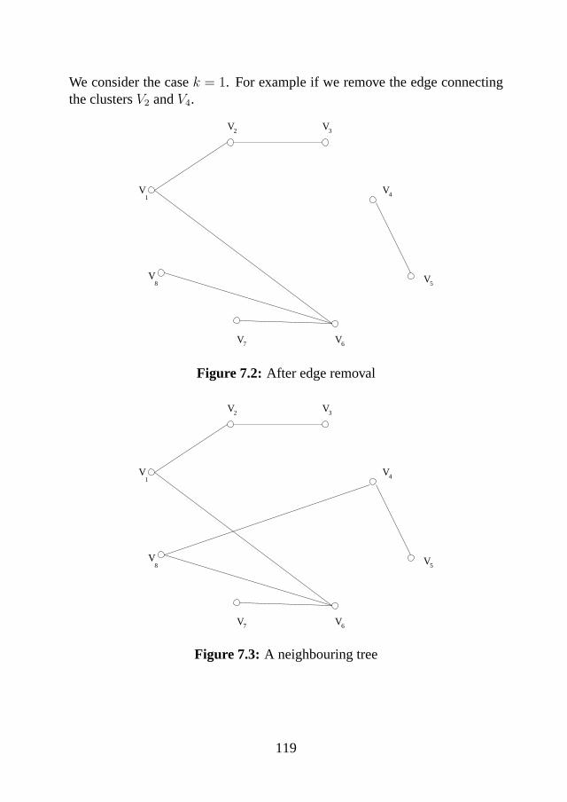
We consider the casek = 1. For example if we remove the edge connectingthe clustersV2 andV4.
V
V8
V V
V
V V
V1
2 3
4
5
67
Figure 7.2: After edge removal
V
8V
V V
V
V V
V1
2 3
4
5
67
Figure 7.3: A neighbouring tree
119

There are several possibilities of reconnecting the two resulting sections toform a valid global tree, for example by connectingV1 with V4 or V2 with V5,etc. All these possibilities of reconnecting give the size of the neighbourhood.
SolvingPlocal(y) with the vectory corresponding to the current neighbouringtree we get a feasible solution for the GMST problem.
Therefore the combination of the definition of feasible solution and neigh-bourhood structure appears to be a good candidate for annealing.
7.5.4 A computational example
Our computational experiment was performed on a HP 9000/735 computerwith a 125 Mhz processor and 144 Mb memory. The Simulated Annealingscheme is written in C and compiled with a HP-UX cc compiler. For solvingthe linear programming problems we used CPLEX.
We consider the GMST problem withm = 10 clusters andn = 3 nodes percluster as an illustration of the simulated annealing method.
We start with the temperatureT0 = 100. The cooling rater = 0.95 will beused to reduce the temperature in each stage, andL = 50 moves evaluatedin each stage. Table 7.1 shows the first twelve iterations of the simulatedannealing procedure.
120
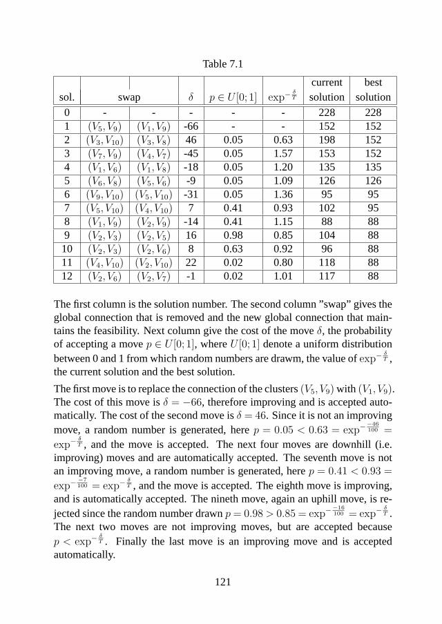
Table 7.1
current bestsol. swap δ p ∈ U [0; 1] exp−
δT solution solution
0 - - - - - 228 2281 (V5, V9) (V1, V9) -66 - - 152 1522 (V3, V10) (V3, V8) 46 0.05 0.63 198 1523 (V7, V9) (V4, V7) -45 0.05 1.57 153 1524 (V1, V6) (V1, V8) -18 0.05 1.20 135 1355 (V6, V8) (V5, V6) -9 0.05 1.09 126 1266 (V9, V10) (V5, V10) -31 0.05 1.36 95 957 (V5, V10) (V4, V10) 7 0.41 0.93 102 958 (V1, V9) (V2, V9) -14 0.41 1.15 88 889 (V2, V3) (V2, V5) 16 0.98 0.85 104 8810 (V2, V3) (V2, V6) 8 0.63 0.92 96 8811 (V4, V10) (V2, V10) 22 0.02 0.80 118 8812 (V2, V6) (V2, V7) -1 0.02 1.01 117 88
The first column is the solution number. The second column ”swap” gives theglobal connection that is removed and the new global connection that main-tains the feasibility. Next column give the cost of the moveδ, the probabilityof accepting a movep ∈ U [0; 1], whereU [0; 1] denote a uniform distributionbetween 0 and 1 from which random numbers are drawm, the value ofexp−
δT ,
the current solution and the best solution.
The first move is to replace the connection of the clusters(V5, V9) with (V1, V9).The cost of this move isδ = −66, therefore improving and is accepted auto-matically. The cost of the second move isδ = 46. Since it is not an improvingmove, a random number is generated, herep = 0.05 < 0.63 = exp−
−46100 =
exp−δT , and the move is accepted. The next four moves are downhill (i.e.
improving) moves and are automatically accepted. The seventh move is notan improving move, a random number is generated, herep = 0.41 < 0.93 =
exp−−7100 = exp−
δT , and the move is accepted. The eighth move is improving,
and is automatically accepted. The nineth move, again an uphill move, is re-jected since the random number drawnp = 0.98 > 0.85 = exp−
−16100 = exp−
δT .
The next two moves are not improving moves, but are accepted becausep < exp−
δT . Finally the last move is an improving move and is accepted
automatically.
121

It is important to observe the large number of non-improving moves that areaccepted in the first stage. In the second stage, the temperature control pa-rameterT is reduced toT = 0.95(100) = 95. This will reduce the probabilityof accepting non-improving moves by five percent. In later stages,T willbecome almost zero and nonimproving moves will be very unlikely to be ac-cepted at all.
It is generally agreed that, relative to special purpose heuristics and othermetaheuristics, simulated annealing requires long runs to reach good solu-tions. Choices of the control parameters and the stopping rule determine thecomputational effort.
122
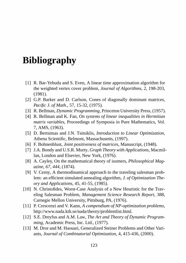
Bibliography
[1] R. Bar-Yehuda and S. Even, A linear time approximation algorithm forthe weighted vertex cover problem,Journal of Algorithms, 2, 198-203,(1981).
[2] G.P. Barker and D. Carlson, Cones of diagonally dominant matrices,Pacific J. of Math., 57, 15-32, (1975).
[3] R. Bellman,Dynamic Programming, Princeton University Press, (1957).[4] R. Bellman and K. Fan,On systems of linear inequalities in Hermitian
matrix variables, Proceedings of Symposia in Pure Mathematics, Vol.7, AMS, (1963).
[5] D. Bertsimas and J.N. Tsitsiklis,Introduction to Linear Optimization,Athena Scientific, Belmont, Massachusetts, (1997).
[6] F. Bohnenblust,Joint positiveness of matrices, Manuscript, (1948).[7] J.A. Bondy and U.S.R. Murty,Graph Theory with Applications, Macmil-
lan, London and Elsevier, New York, (1976).[8] A. Cayley, On the mathematical theory of isomers,Philosophical Mag-
azine, 67, 444, (1874).[9] V. Cerny, A thermodinamical approach to the traveling salesman prob-
lem: an efficient simulated annealing algorithm,J. of Optimization The-ory and Applications, 45, 41-55, (1985).
[10] N. Christofides, Worst-Case Analysis of a New Heuristic for the Trav-eling Salesman Problem,Management Science Research Report, 388,Carnegie Mellon University, Pittsburg, PA, (1976).
[11] P. Crescenzi and V. Kann,A compendium of NP-optimization problems,http://www.nada.kth.se/nada/theory/problemlist.html.
[12] S.E. Dreyfus and A.M. Law,The Art and Theory of Dynamic Program-ming, Academic Press, Inc. Ltd., (1977).
[13] M. Dror and M. Haouari, Generalized Steiner Problems and Other Vari-ants,Journal of Combinatorial Optimization, 4, 415-436, (2000).
123
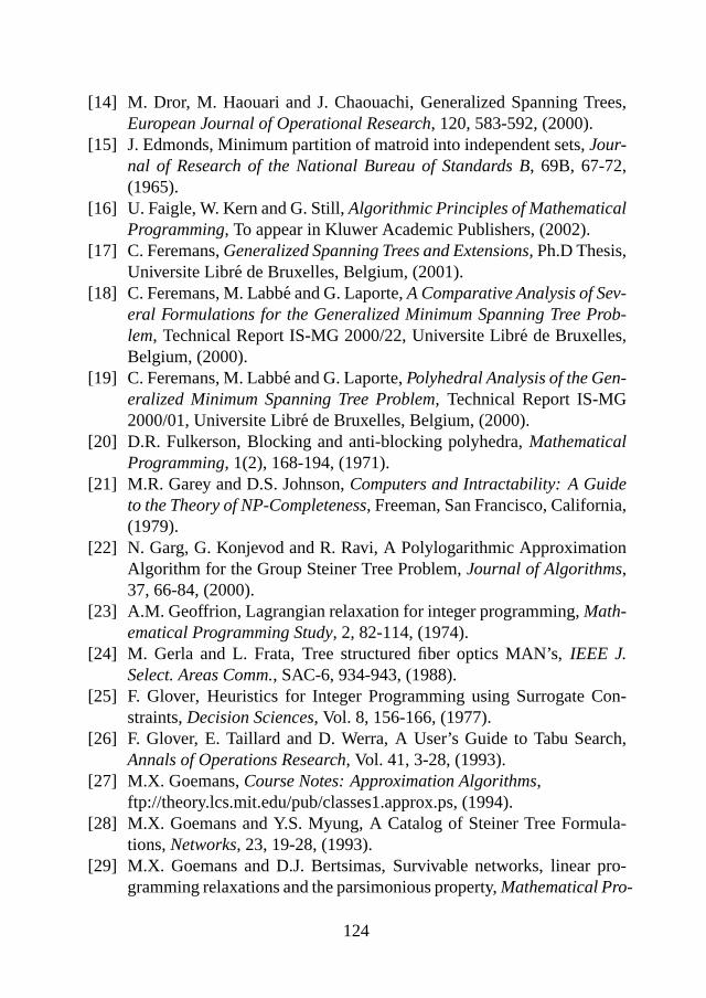
[14] M. Dror, M. Haouari and J. Chaouachi, Generalized Spanning Trees,European Journal of Operational Research, 120, 583-592, (2000).
[15] J. Edmonds, Minimum partition of matroid into independent sets,Jour-nal of Research of the National Bureau of Standards B, 69B, 67-72,(1965).
[16] U. Faigle, W. Kern and G. Still,Algorithmic Principles of MathematicalProgramming, To appear in Kluwer Academic Publishers, (2002).
[17] C. Feremans,Generalized Spanning Trees and Extensions, Ph.D Thesis,Universite Libre de Bruxelles, Belgium, (2001).
[18] C. Feremans, M. Labbe and G. Laporte,A Comparative Analysis of Sev-eral Formulations for the Generalized Minimum Spanning Tree Prob-lem, Technical Report IS-MG 2000/22, Universite Libre de Bruxelles,Belgium, (2000).
[19] C. Feremans, M. Labbe and G. Laporte,Polyhedral Analysis of the Gen-eralized Minimum Spanning Tree Problem, Technical Report IS-MG2000/01, Universite Libre de Bruxelles, Belgium, (2000).
[20] D.R. Fulkerson, Blocking and anti-blocking polyhedra,MathematicalProgramming, 1(2), 168-194, (1971).
[21] M.R. Garey and D.S. Johnson,Computers and Intractability: A Guideto the Theory of NP-Completeness, Freeman, San Francisco, California,(1979).
[22] N. Garg, G. Konjevod and R. Ravi, A Polylogarithmic ApproximationAlgorithm for the Group Steiner Tree Problem,Journal of Algorithms,37, 66-84, (2000).
[23] A.M. Geoffrion, Lagrangian relaxation for integer programming,Math-ematical Programming Study, 2, 82-114, (1974).
[24] M. Gerla and L. Frata, Tree structured fiber optics MAN’s,IEEE J.Select. Areas Comm., SAC-6, 934-943, (1988).
[25] F. Glover, Heuristics for Integer Programming using Surrogate Con-straints,Decision Sciences, Vol. 8, 156-166, (1977).
[26] F. Glover, E. Taillard and D. Werra, A User’s Guide to Tabu Search,Annals of Operations Research, Vol. 41, 3-28, (1993).
[27] M.X. Goemans,Course Notes: Approximation Algorithms,ftp://theory.lcs.mit.edu/pub/classes1.approx.ps, (1994).
[28] M.X. Goemans and Y.S. Myung, A Catalog of Steiner Tree Formula-tions,Networks, 23, 19-28, (1993).
[29] M.X. Goemans and D.J. Bertsimas, Survivable networks, linear pro-gramming relaxations and the parsimonious property,Mathematical Pro-
124

gramming, 60, 145-166, (1993).[30] M. Grotschel,Discrete mathematics in manufacturing, Preprint SC 92-
3, ZIB, (1992).[31] M. Grotschel, L. Lovasz and A. Schrijver,Geometric Algorithms and
Combinatorial Optimization, Springer-Verlag, Berlin, (1988).[32] M. Grotschel, L. Lovasz and A. Schrijver, The ellipsoid method and its
consequences in combinatorial optimization,Combinatorica, 1, 169-197, (1981).
[33] M. Held and R.M. Karp, The traveling salesman problem and minimumspanning trees,Operations Research, 18, 1138-1162, (1970).
[34] M. Held and R.M. Karp, The traveling salesman problem and minimumspanning trees: part II,Mathematical Programming, 1, 6-25, (1971).
[35] C.S. Helvig, G. Robins and A. Zelikovsky, An Improved Approxima-tion Scheme for the Group Steiner Problem,Networks, 37, Issue 1, 8-20,(2001).
[36] A.L. Henry-Labordere, The Record Balancing Problem: A DynamicProgramming Solution of a Generalized Traveling Salesman Problem,RIRO, B-2, 43-49, (1969).
[37] J.B. Hiriart-Urruty and C. Lemarechal,Convex Analysis and Minimiza-tion Algorithms II, Springer-Verlag, Berlin, (1993).
[38] D. Hochbaum, Approximation algorithms for set covering and vertexcover problems,SIAM Journal of Computing, 11, 555-556, (1982).
[39] J.H. Holland,Adaptation in Natural and Artificial Systems, Universityof Michigan Press, Ann Arbor, (1975).
[40] E. Ihler, G. Reich and P. Widmayer, Class Steiner Trees and VLSI-design,Discrete Applied Mathematics, 90, 173-194, (1999).
[41] D. Johnson, C. Aragon, L. McGeoch and C. Schevon, Optimizationby Simulated Annealing: An Experimental Evaluation, Part I, GraphPartitioning,Operations Research, 37, 865-892, (1989).
[42] N. Karmarkar, A new polynomial-time algorithm in linear program-ming,Combinatorica, 4, 373-395, (1979).
[43] L.G. Khachiyan, A polynomial algorithm in linear programming,SovietMathematics Doklady, 191-194, (1979).
[44] S. Kirkpatrick, C.D.. Gelatt and M.D. Vecchi, Optimization by Simu-lated Annealing,Science, Vol. 220, No. 4598, 671-680, (1983).
[45] J.B. Kruskal,On the shortest spanning subtree of a graph and the trav-eling salesman problem, Proceedings of the American MathematicalSociety 7, 48-50, (1956).
125

[46] G. Laporte, H. Mercure and Y. Norbert, Finding the Shortest Hamilto-nian Circuit through n Clusters: a Lagrangian Approach,CongressusNumerantium, 48, 277-290, (1985).
[47] G. Laporte, H. Mercure and Y. Norbert, Generalized Traveling Sales-man Problem through n Sets of Nodes: The asymmetrical Case,Dis-crete Applied Mathematics, 18, 185-197, (1987).
[48] C. Lemarechal and F. Oustry,Semidefinite relaxations and Lagrangianduality with application to combinatorial optimization, Rapport de recher-che, N. 3710, INRIA Rhone-Alpes, France, (1999).
[49] L. Lovasz and A. Schrijver, Cones of matrices and set-functions and 0-1optimization,SIAM J. Optim., 1(2): 166-190, (1991).
[50] L. Lovasz, On some connectivity properties of Eulerian graphs,ActaMathematica Academiae Scientiarum Hungaricae, 28, 129-138, (1976).
[51] T.L. Magnanti and L.A. Wolsey,Optimal Trees, Handbooks in Opera-tions Research & Management Science, M.O. Ball, T.L. Magnanti, C.L.Monma, G.L. Nemhauser (Editors), Elsevier Science, Amsterdam, Vol.7, chap. 9, 503-615, (1995).
[52] N. Metropolis, A. Rosenbluth, M. Rosenbluth, A. Teller and E. Teller,Equations of State Calculations by Fast Computing Machines,Journalof Chemical Physics, Vol. 21, No. 6, 1087-1092, (1953).
[53] R.D.C. Monteiro and S. Zhang, A unified analysis for a class of long-step primal-dual path-following interior-point algorithms for semidefi-nite programming,Math. Programming, 81, 281-299, (1998).
[54] Y.S. Myung, C.H. Lee and D.w. Tcha, On the Generalized MinimumSpanning Tree Problem,Networks, 26, 231-241, (1995).
[55] G.L. Nemhauser and L.A. Wolsey,Integer and Combinatorial Opti-mization, John Wiley & Sons, New York, Reprint of the 1988 original,(1999).
[56] I.H. Osman and G. Laporte, Metaheuristics: A Bibliography,Annals ofOperations Research, 63, 513-623, (1996).
[57] C.H. Papadimitriou and K. Steiglitz,Combinatorial Optimization: Al-gorithms and Complexity, Prentice-Hall, Englewood Cliffs, New Jersey,(1982).
[58] R.C. Prim, Shortest connection networks and some generalizations,BellSystems Technical Journal, 36, 1389-1401, (1957).
[59] J.J. Prisco, Fiber optic regional area networks in New York and Dallas,IEEE J. Select. Areas Comm., SAC-4, 750-757, (1986).
[60] P.C. Pop, U. Faigle, W. Kern and G. Still,Relaxation methods for the
126
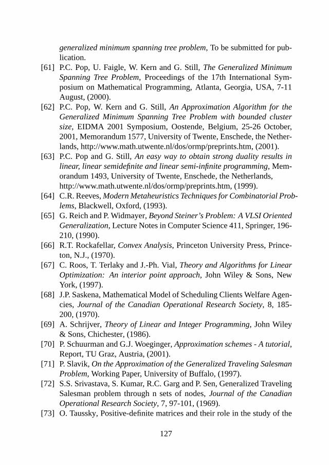
generalized minimum spanning tree problem, To be submitted for pub-lication.
[61] P.C. Pop, U. Faigle, W. Kern and G. Still,The Generalized MinimumSpanning Tree Problem, Proceedings of the 17th International Sym-posium on Mathematical Programming, Atlanta, Georgia, USA, 7-11August, (2000).
[62] P.C. Pop, W. Kern and G. Still,An Approximation Algorithm for theGeneralized Minimum Spanning Tree Problem with bounded clustersize, EIDMA 2001 Symposium, Oostende, Belgium, 25-26 October,2001, Memorandum 1577, University of Twente, Enschede, the Nether-lands, http://www.math.utwente.nl/dos/ormp/preprints.htm, (2001).
[63] P.C. Pop and G. Still,An easy way to obtain strong duality results inlinear, linear semidefinite and linear semi-infinite programming, Mem-orandum 1493, University of Twente, Enschede, the Netherlands,http://www.math.utwente.nl/dos/ormp/preprints.htm, (1999).
[64] C.R. Reeves,Modern Metaheuristics Techniques for Combinatorial Prob-lems, Blackwell, Oxford, (1993).
[65] G. Reich and P. Widmayer,Beyond Steiner’s Problem: A VLSI OrientedGeneralization, Lecture Notes in Computer Science 411, Springer, 196-210, (1990).
[66] R.T. Rockafellar,Convex Analysis, Princeton University Press, Prince-ton, N.J., (1970).
[67] C. Roos, T. Terlaky and J.-Ph. Vial,Theory and Algorithms for LinearOptimization: An interior point approach, John Wiley & Sons, NewYork, (1997).
[68] J.P. Saskena, Mathematical Model of Scheduling Clients Welfare Agen-cies, Journal of the Canadian Operational Research Society, 8, 185-200, (1970).
[69] A. Schrijver,Theory of Linear and Integer Programming, John Wiley& Sons, Chichester, (1986).
[70] P. Schuurman and G.J. Woeginger,Approximation schemes - A tutorial,Report, TU Graz, Austria, (2001).
[71] P. Slavik,On the Approximation of the Generalized Traveling SalesmanProblem, Working Paper, University of Buffalo, (1997).
[72] S.S. Srivastava, S. Kumar, R.C. Garg and P. Sen, Generalized TravelingSalesman problem through n sets of nodes,Journal of the CanadianOperational Research Society, 7, 97-101, (1969).
[73] O. Taussky, Positive-definite matrices and their role in the study of the
127
characteristic roots of general matrices,Advances in Math., 2, 175-186,(1968).
[74] M.J. Todd, A study of search directions in primal-dual interior-pointmethods for semidefinite programming,Optim. Methods Softw., 11&12,1-46, (1999).
[75] V.V. Vazirani,Approximation Algorithms, Springer Verlag, Berlin, (2001).[76] H. Wolkowicz, R. Saigal, and L. Vandenberghe (editors).Handbook on
Semidefinite Programming, Kluwer, (2000).[77] B.J. Wythoff, Backpropagation Neural Networks. A Tutorial,Chemo-
metrics and Intelligent Laboratory Systems, 18, 115-155, (2001).[78] M. Yannakakis, Expressing combinatorial optimization problems by
linear programs,Journal of Computer and System Sciences, 43, 441-466, (1991).
128

Subject Index
Aalgorithm, 3
approximation, 3ellipsoid, 10exact, 3exponential time, 4greedy, 18heuristic, 3non-deterministic, 4polynomial time, 4
algorithm of Kruskal, 19algorithm of Prim, 20annealing
algorithm, 122schedule, 119
arc, 12incoming, 12outcoming, 12
Artificial Neural Networks, 119
Bbidirectional flow formulation, 44bidual, 94binary variable, 2branching model, 40
Ccapacity function, 12cluster
bounded size, 68clusters, 16combination
affine, 8convex, 8
combinatorial optimization, 2complementary slackness, 90complexity theory, 3component, 11
even, 11odd, 11
concave function, 84piecewise linear, 84
conehomogeneous, 87of positive semidefinite matri-
ces, 87selfpolar, 87
conic programming, 87connection
global, 47local, 47
constraintscluster subpacking, 45integrality, 82quadratic, 96
control parameter, 125convex, 8
129
cone, 8cooling
rate, 123schedule, 125
cost functionstrict positive, 68triangle inequality, 68
cut, 12cutset, 11cycle, 11
Ddecision problem, 4decisions
generic, 123problem specific, 123
dimension of a polyhedron, 9directed
generalized cutset formulation,37
multicommodity flow model, 42dual problem, 94duality gap, 81dualization, 96
boolean, 99complete, 97linear, 97
dynamic programming, 7backward, 7forward, 7
Eedge set, 10edges, 10
adjacent, 11EXP, 4
Ffeasible solution set, 2
flow, 12value, 12
forest, 11
GGeneralized
Minimum Spanning Tree Prob-lem, 16
Steiner Tree Problem, 16Traveling Salesman Problem, 18
generalizedcutset formulation, 34multicut formulation, 36spanning tree, 20structure, 16subtour elimination formulation,
33Genetic Algorithms, 119GMST, 20graph, 10
complete, 11connected, 11contracted, 47directed, 12
Group Steiner Tree Problem, 16
Hhyperplane, 9
separating, 9
Iinner product, 87input, 3integer programming problem, 2integrality property, 83interior point methods, 10iterative improvement, 116
Kk-neighbourhood, 127
130

Karmakar’s algorithm, 70
LLowner partial order, 87Lagrangian
dual function, 81dual problem, 81multipliers, 81relaxation, 81
leaf, 11lifting procedure, 95linear programming, 3linearly independent, 8local
optimal, 117search, 116
local solution, 47local-global formulation, 50
Mmatrix
diagonal, 97positive semidefinite, 87pseudo-inverse, 91symmetric, 87
max-flow min-cut theorem, 13maximum flow problem, 12metaheuristic, 118Metropolis’ algorithm, 121minimum spanning tree problem, 4mixed integer programming prob-
lem, 2multigraph, 11
Nneighbor, 11neighbourhood, 117node
cover, 12
isolated, 11parent, 25
node cover problem, 21node set, 10nodes, 10
adjacent, 10NP, 4NP-complete, 5NP-hard, 5
Oobjective function, 2optimal solution, 116
PP, 4parsimonious property, 71partition, 16path, 11performance
average-case, 60experimental, 61guarantee, 62worst-case, 61
polyhedron, 9bounded, 9rational, 9
polynomial reduction, 5polynomially transformable, 5polytope, 9positive semidefinite, 6primal-dual methods, 64principle of optimality, 8
Qquadratic function, 91
Rrange of a matrix, 91
131
rank of a matrix, 9relaxation, 63
Lagrangian, 6linear programming, 6semidefinite programming, 6
root, 25rooting procedure, 52rounding, 63running time, 3
SSchur’s Lemma, 92semidefinite programming, 86separation
algorithm, 9problem, 9
set cover, 25problem, 25
Simulated Annealing, 119single commodity model, 42size, 3Slater-type constraint qualification,
88solution
feasible, 10local, 3optimal, 10sub-optimal, 116
strong duality theorem, 90subdifferential, 84subgradient, 84
optimization algorithm, 85subgraph, 11
induced, 11survivable network design problem,
70
TTabu Search, 119
traceinner product, 87
tree, 11minimum spanning, 18rooted, 25spanning, 12
Uundirected
graph, 20multicommodity flow model, 45
undirected cluster subpacking for-mulation, 46
Vvertex, 9
Wweak duality theorem, 82worst-case ratio, 62
132

Summary
Classical combinatorial optimization problems can often be generalized in anatural way by considering a related problem relative to a given partition ofthe nodes into clusters.
We study various relaxation and heuristic techniques in the special case ofthe so-called Generalized Minimum Spanning Tree (GMST) problem. In theGMST problem given an undirected graph with nodes partitioned into clus-ters and edges defined between nodes belonging to different clusters with anonnegative cost, we search for a minimum cost tree spanning a subset ofnodes which includes exactly one node from each cluster. This problem wasintroduced by Myung, Lee and Tcha [54], they also proved that the problemis NP-hard. The last result is a direct consequence of one of our results inwhich we prove that the GMST problem on trees isNP-hard. We presentalso two cases when the GMST problem is solvable in polynomial time.
We present new integer and mixed integer programming formulations for theGMST problem and we compare them in terms of their linear programmingrelaxations with the formulations already proposed in the literature.
Based on a new formulation of the problem called local-global formulation,we present a new solution procedure. Our procedure called rooting proce-dure is compared with the procedures developed by Myunget al. [54] andby Feremans [17]. For all instances of the problem that we considered, theoptimal solution of the GMST problem has been found. As far as we know,our method is the second method, after Feremans [17], which solves instanceswith more than 120 nodes to optimality, but the computing times spent by thebranch and cut code proposed in [17] are in general larger than the times spentby our rooting procedure code.
We compare the bound provided by the linear programming relaxation of ageneral 0-1 programming problem with the bounds obtained by considering
133

the linear, complete and boolean dualizations suggested in [48]. We applythe theoretical results obtained to the GMST problem. In the Lagrangianrelaxation that we considered, a set of inequalities in the bidirectional mul-ticommodity flow formulation of the problem is dualized and added to theobjective function. We used the subgradient optimization algorithm to obtainlower bounds. Computational results are reported for many instances of theproblem.
We distinguish in Chapter 4 between so-called positive and negative resultsin the area of approximation algorithms. We present an in-approximabilityresult: there is noα-approximation algorithm for the GMST problem unlessP = NP . Our result is a formulation in terms of approximation algorithmsof a result of Myunget al. [54]. However, under special assumptions (seeSection 4.4) we give an approximation algorithm for the GMST problem.
In the last chapter of this thesis we present basic theory of heuristic algorithmsand local search and solve the GMST problem with Simulated Annealing.
134