the generalized likelihood uncertainty estimation · pdf filechapter 4 the generalized...

CHAPTER 4

The Generalized LikelihoodUncertainty Estimationmethodology

Calibration and uncertainty estimation based upon a statistical framework isaimed at finding an optimal set of models, parameters and variables capable ofsimulating a given system.

There are many possible sources of mismatch between observed and simulatedstate variables (see section 3.2). Some of the sources of uncertainty originatefrom physical randomness, and others from uncertain knowledge put into thesystem. The uncertainties originating from physical randomness may be treatedwithin a statistical framework, whereas alternative methods may be needed toaccount for uncertainties originating from the interpretation of incomplete andperhaps ambiguous data sets.

The GLUE methodology (Beven and Binley 1992) rejects the idea of one singleoptimal solution and adopts the concept of equifinality of models, parametersand variables (Beven and Binley 1992; Beven 1993). Equifinality originates fromthe imperfect knowledge of the system under consideration, and many sets ofmodels, parameters and variables may therefore be considered equal or almostequal simulators of the system. Using the GLUE analysis, the prior set of mod-els, parameters and variables is divided into a set of non-acceptable solutions anda set of acceptable solutions. The GLUE methodology deals with the variabledegree of membership of the sets. The degree of membership is determined byassessing the extent to which solutions fit the model, which in turn is determined

53

CHAPTER 4. THE GENERALIZED LIKELIHOOD UNCERTAINTY ESTIMATIONMETHODOLOGY

by subjective likelihood functions. By abandoning the statistical framework wealso abandon the traditional definition of uncertainty and in general will have toaccept that to some extent uncertainty is a matter of subjective and individualinterpretation by the hydrologist. There are strong parallels between uncertaintyin a Fuzzy set ruled system and uncertainty in the GLUE methodology. Fuzzylogic is an alternative or supplement to the classical probabilistic frameworkin situations where very little information is available, and such informationas there is tends to be ambiguous and vague. Considering the sources of mis-match between observed and simulated state variables (see section 3.2), it canbe argued that the mismatch is to a great extent due to vague and ambiguousinterpretations.

The GLUE methodology consists of the 3 steps described below (Fig. 4.1).

Sample parameter set

Groundwater model

System stage

System input

Comparison with observed data

Unconditional stochastic output

Probability density funct

Deteministic model

Stochastic model

GLUE procedure

OK Yes

RejectedL( )=0

Simulation accepted with weight - L()

No

Input Output

f( 1)

1

f( 1)

1

Prior statistics

f( 2)

2

f( N)

N

f( 2)

2

f( M )

M

Probability density functions

fp( 1)

1

fp( 2)

2

M

fp( N)

fp( 1)

1

fp( 2)

2

N

fp( N)

Posterior statistics

(a)

(c)

(d)

(e)

(b)

(f)

Figure 4.1: The GLUE procedure. (a) prior statistics, (b) stochastic modelling, (c)unconditional statistics of system state variables, (d) evaluation procedure(e) posterior parameter likelihood functions and (f) likelihood functions forsystem state variables

Step 1 is to determine the statistics for the models, parameters and variables

54

4.1. LIKELIHOOD MEASURES

that, prior to the investigation, are considered likely to be decisive for the sim-ulation of the system (a). Typically quite wide discrete or continuous uniformdistribution is chosen - reflecting the fact that there is little prior knowledge ofthe uncertainties arising from models, parameters and variables. In principle allavailable knowledge can be put into the prior distributions.

Step 2 is a stochastic simulation (b) based on the models, parameters and vari-ables defined in step 1. The Monte Carlo or Latin Hypercube method (AppendixA) may be used to do a random sample of the parameter sets. Step 2 gives usan unconditional estimate of the statistics of any system state variable (c).

In step 3 an evaluation procedure (d) is carried out for every single simulationperformed in step 2. Simulations and thus parameter sets are rated according tothe degree to which they fit observed data. If the simulated state variables are“close” to the observed values the simulation is accepted as having a given likeli-hood L(θ|ψ), whereas if the considered simulated state variables are unrealisticthe simulation is rejected as having zero likelihood.

In this way a likelihood value is assigned to all accepted parameter sets (zerofor rejected sets and positive for accepted sets). The direct result of this is adiscrete joint likelihood function (DJPDF) for all the models, parameters andvariables involved. The DJPDF can only be illustrated in two, maximum three,dimensions, and likelihood scatter plots are often used to illustrate the estimatedparameters, see e.g. Fig. 5.7. In Fig. 4.1 the models, parameters and variablesθ1, ..., θi, ..., θN are considered independent, the likelihood is projected onto theparameter axis, and discrete density functions (e) are presented, see section 4.3.Discrete likelihood functions for all types of system state variables can likewisebe constructed (f).

4.1 Likelihood measures

Likelihood is a measure of how well a given combination of models, parametersand variables fits, based on the available set of observations. The likelihoodmeasure thus describes the degree to which the various acceptable solutions aremembers of the set, i.e. their degree of membership.

The calculation of the likelihood of a given set of models, parameters and vari-ables is the key feature of the GLUE methodology, and in this respect GLUEdiffers from the classical methods of calibration and uncertainty estimation. Aswill be seen in what follows a wide range of likelihood measures are suggested -all with different qualities. There are no definitive rules for choosing a certainlikelihood measure. Some personal preferences are however mentioned in section4.2.

55


The likelihood measure consists, in this thesis, of three elements: 1) a rejectionlevel that indicates whether the acceptance criteria are fulfilled or not, 2) apoint likelihood measure that sums up the degree of model fit in the individualobservation points and 3) a global likelihood measure that is an aggregation ofall the point likelihood measures.

Often the rejection level is implicitly given in the point likelihood function, andoccasionally the rejection level, the point likelihood measure and the global like-lihood measure are all gathered in one function.

The likelihood functions presented below in Fig. 4.2 are based on a combinationof the likelihood functions derived from the classical statistical framework andfrom GLUE, and the Fuzzy logic literature.

Figure 4.2: a) Gaussian likelihood function , b) model efficiency likeli-hood function, c) inverse error variance likelihood function,d) trapezoidal likelihood function, e) triangular likelihoodfunction and f) uniform likelihood function

4.1.1 Traditional statistical likelihood measures

Gaussian likelihood function

The Gaussian likelihood function, Fig. 4.2a, is often used in a classical statisticalframework. The residuals are assumed to be Gaussian and the likelihood equalsthe probability that the simulated value, ψi(θ), equals the observed value, ψ∗

i :

56


L (θ|ψ∗i ) =

1√2πσψ∗

i

e−(

(ψ∗i−ψi(θ))

2

2σ2ψ∗i

)(4.1)

or for Nobs observations

L (θ|ψ∗) = (2π)Nobs

2 | Cψ∗ |− 12 e(

12 (ψ∗−ψ(θ))TC−1

ψ∗ (ψ∗−ψ(θ))) (4.2)

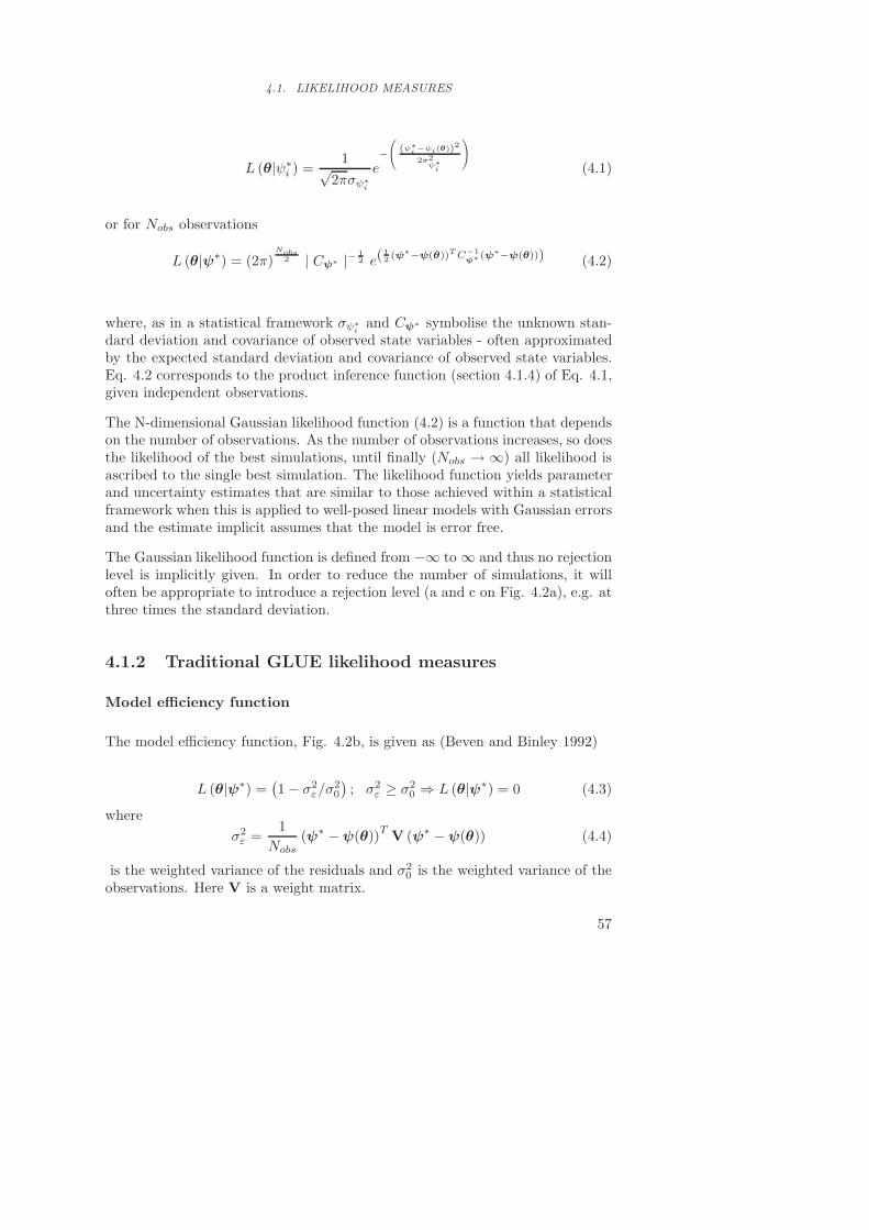
where, as in a statistical framework σψ∗i

and Cψ∗ symbolise the unknown stan-dard deviation and covariance of observed state variables - often approximatedby the expected standard deviation and covariance of observed state variables.Eq. 4.2 corresponds to the product inference function (section 4.1.4) of Eq. 4.1,given independent observations.

The N-dimensional Gaussian likelihood function (4.2) is a function that dependson the number of observations. As the number of observations increases, so doesthe likelihood of the best simulations, until finally (Nobs → ∞) all likelihood isascribed to the single best simulation. The likelihood function yields parameterand uncertainty estimates that are similar to those achieved within a statisticalframework when this is applied to well-posed linear models with Gaussian errorsand the estimate implicit assumes that the model is error free.

The Gaussian likelihood function is defined from −∞ to ∞ and thus no rejectionlevel is implicitly given. In order to reduce the number of simulations, it willoften be appropriate to introduce a rejection level (a and c on Fig. 4.2a), e.g. atthree times the standard deviation.

4.1.2 Traditional GLUE likelihood measures

Model efficiency function

The model efficiency function, Fig. 4.2b, is given as (Beven and Binley 1992)

L (θ|ψ∗) =(1 − σ2

ε/σ20

); σ2

ε ≥ σ20 ⇒ L (θ|ψ∗) = 0 (4.3)

whereσ2ε =

1Nobs

(ψ∗ −ψ(θ))T V (ψ∗ −ψ(θ)) (4.4)

is the weighted variance of the residuals and σ20 is the weighted variance of the

observations. Here V is a weight matrix.

57


The likelihood equals one if all residuals are zero, and zero if the weighted vari-ance of the residuals is larger then the weighted variance of the observations.

Inverse error variance function

Beven and Binley (1992) have suggested a function based on the inverse errorvariance with shaping factor N , Fig. 4.2c:

L (θ|ψ∗) =(σ2ε

)−N(4.5)

This function concentrates the weights of the best simulations as N increases.For N → ∞ all weight will be on the single best simulation and for small valuesof N all simulations will tend to have equal weight.

4.1.3 Fuzzy likelihood measures

A point observation of the ith system state variable, ψ∗i , and a computed value

of the same system state variable, ψi(θ) are considered. In the set of all possiblevalues of ψi, a subset, Ψi, is defined where the transition between membershipand non-membership is gradual. The likelihood - or, in Fuzzy terms, the degreeof membership - is maximum for simulated state variables that belong completelyto Ψi; elsewhere it is between 0 and the maximum value. In Fuzzy logic Ψi iscalled a fuzzy set and the likelihood (degree of membership) is described by thelikelihood function (membership function), �LΨi . The likelihood function can inprinciple be an arbitrary, non-symmetric and biased function. The trapezoidal,triangular and uniform likelihood functions are typical Fuzzy logic membershipfunctions where the likelihood or degree of membership is evaluated throughrelatively simple functions.

First the point likelihood measures are described, and then the point likelihoodmeasures are combined through the so-called inference functions.

Trapezoidal likelihood function

The trapezoidal likelihood function, Fig. 4.2d, is given as

L (θ|ψ∗i ) =

ψi(θ) − a

b− aIa,b(ψi(θ)) + Ib,c(ψi(θ)) +

d− ψi(θ)d− c

Ic,d(ψi(θ)) (4.6)

where58


Ia,b =

{1 if a ≤ ψi(θ) ≤ b

0 otherwise

Ib,c =

{1 if b ≤ ψi(θ) ≤ c

0 otherwise

Ic,d =

{1 if c ≤ ψi(θ) ≤ d

0 otherwise

Triangular likelihood function

The triangular likelihood function, Fig. 4.2e, is given as

L (θ|ψ∗i ) =

ψi(θ) − a

b− aIa,b(ψi(θ)) +

c− ψi(θ)c− b

Ib,c(ψi(θ)) (4.7)

where

Ia,b =

{1 if a ≤ ψi(θ) ≤ b

0 otherwise

Ib,c =

{1 if b ≤ ψi(θ) ≤ c

0 otherwise

Uniform likelihood function

The uniform likelihood function, Fig. 4.2f, is a special case of the trapezoidallikelihood function where a = b and c = d.

L (θ|ψ∗i ) =

{1 if a < ψ∗

i − ψi(θ) < b

0 otherwise(4.8)

4.1.4 Inference functions

The overall combination of the individual point likelihood (degree of member-ship) for the observation points is assembled through the so-called degree offulfilment (DOF) (Dubois and Prade 1980), which, in this context, is the overalllikelihood value for the simulation - a global likelihood measure, L (θ|ψ∗). Aclassification of aggregation operators used in Fuzzy rules systems is given inZimmermann (1991), p. 40-41, and some relevant operators are given below(Dubois and Prade 1980; Zimmermann 1991):

59


Product inference

L (θ|ψ∗) =Nobs∏i=1

L (θ|ψ∗i ) (4.9)

The product inference is very restrictive - if one observation is outside the Fuzzyset, Ψ, (i.e. rejected) the global likelihood will be zero. As Nobs increases, theglobal likelihood response surface becomes steeper and steeper and as Nobs → ∞all except the single best simulation will have negligible likelihood.

Min. inference

L (θ|ψ∗) = mini=1,...,Nobs

L (θ|ψ∗i ) (4.10)

The min. inference is as restrictive as the product inference function but theglobal likelihood response surface is more flat.

Max. inference

L (θ|ψ∗) = maxi=1,...,Nobs

L (θ|ψ∗i ) (4.11)

The max. inference is the least restrictive inference function. The likelihood isevaluated from the observation point with the best agreement. If just one ob-servation is inside the Fuzzy set (i.e. accepted), then the simulation is accepted.

Weighted arithmetic mean inference

L (θ|ψ∗) =1

Nobs

Nobs∑i=1

ωiL (θ|ψ∗i ) (4.12)

where ωi is the weight on the ith observation.

As in the case of max. inference, the inclusion of just one observation within theaccepted set will result in acceptance of the simulation. The response surface forthe arithmetic mean inference is very flat.

60


Geometric mean inference

L (θ|ψ∗) = Nobs

√√√√Nobs∏i=1

L (θ|ψ∗i ) (4.13)

The geometric mean inference is as restrictive as the product and min. inference,but the likelihood response surface is less steep. The function is independent ofthe number of observations.

The way that a likelihood calculation might be performed when different typesof observation data are available is illustrated in example 4.1 below.

Example 4.1 A stationary groundwater model is constructed for a river catch-ment. The model is calibrated to a summer situation. The following observationsare available:

• Head observations in 16 wells. From initial studies the standard error onthe observed heads is estimated to be 1.5 m. Trapezoidal likelihood functionsare applied. Fig. 4.3(a)

• Median value of annual minimum discharge observations at one station in“Large Creek”. The estimation error is assumed to be Gaussian with astandard error of 10 % of measured discharge. The rejection level is threetimes standard error. Fig. 4.3(b)

• A local farmer has stated that “Little Creek dries out every summer”. Wedo not rely totally on this statement and formulate a likelihood functionthat gradually decreases from 0 l/s to 2.0 l/s. Fig. 4.3(c)

• Information from the local waterworks indicates that so far abstraction wellno. 12 has never dried out. Low hydraulic conductivities may result in theclosing of abstraction wells in the numerical model. Seen in the light of theinformation given above, every simulation where the abstraction is closedmust be unrealistic, and consequently the likelihood is set at zero. Fig.4.3(d)

In all, 19 observations are available and they are combined into an global simula-tion likelihood measure by an inference rule, e.g. weighted arithmetic mean, Eq.4.12, or geometric mean inference, Eq. 4.13. Alternatively two or more rulescan be combined, e.g. Eq. 4.14.

L (θ|ψ∗) = ωhead116

∑16i=1 Lh∗

i(hi(θ)) · ωq1Lq∗1 (q1(θ))

·ωq2Lq∗2 (q2(θ)) · ωAbsLAbs∗2 (Abs(θ))(4.14)

61


hi hi +1.5 hi + 4.5 q q + 30%q - 30%hi -1.5hi - 4.5

open closed

1

head [m] "Large Creek"discharge [l/s]

0 0.5 1.0 1.5

"Little Creek"summer discharge[l/s]

Status,Abstraction site #

1

11

(a) (b)

(c) (d)

Figure 4.3: Examples of different likelihood functions

where ωhead, ωq1 , ωq2 and ωAbs are the weight on observed head data, observeddischarge in “Little Creek”, observed discharge in “Large Creek” and waterworksobservation respectively. Lh∗

i(hi(θ)), Lq∗1 (q1(θ)), Lq∗2 (q2(θ)) and LAbs∗2 (Abs2(θ))

are likelihood functions for head data, discharge in “Little Creek”, discharge in“Large Creek” and the abstraction respectively.

4.2 Designing the likelihood measure

The GLUE methodology is aimed at finding possible sets of models, param-eters and variables which produce a model output that is in agreement withobservations. The likelihood measure reflects the degree to which we accept thesimulated output to deviate from observations due to the numerous error sources.

The first step in the construction of the likelihood function is to analyse possiblesources of mismatch between observed and simulated state variables. Section3.2 is a description of the different types of observation data and a descriptionof the different sources of mismatch between observed and simulated values.Section 3.2 may be used as a guideline in estimating the expected standarderrors of observation. In reviewing the possible errors, the hydrologist is forcedto consider what is included in the model and what is not. E.g. if the purposeof the model is to model small-scale point pollution, small-scale heterogeneityis very important and consequently has to be modelled in such a way that theerror contribution from ignored small-scale heterogeneities will be very small.

In the opinion of the author the estimated expected error should be closelyrelated to the likelihood measure. The rejection level may be three times theexpected standard error, reflecting a very low probability of larger errors: see

62

4.3. BAYESIAN UPDATING OF PRIOR PARAMETER DISTRIBUTIONS

Chapters 5 and 6

The second step in the calculation of the likelihood measure is the combinationof the individual point likelihood measures into a global likelihood measure.

The aim of the point likelihood measures is to account for all expected uncer-tainty, and in the author’s opinion therefore the simulation can be accepted onlyif all point observations are accepted - no simulated state variables can be tol-erated outside the rejection level. If this results in an over-restrictive likelihoodmeasure, the point likelihood measures, and thus the expected errors, should bereconsidered, and if there is no objective reason for increasing the amount ofexpected error the model should be reconsidered.

The min. inference, the product inference and the geometric mean inferencefunction fulfil the requirement listed above (all point likelihood measures haveto be positive in order to accept the simulation).

The geometric mean inference function is attractive because the likelihood mea-sure is independent of the number of observations. This means that the uncer-tainty estimate does not improve if the number of observations is doubled. Thisbehaviour contrasts with the classical regression framework, where it is assumedthat the estimation error is reduced as the number of observations increases.Actually, the maximum likelihood estimate for N independent parameters is theproduct inference of the independent maximum likelihood estimate.

The reason why the geometric mean inference function is found attractive lieswithin the error sources. From section 3.2 it can be seen that the main er-ror contributions (scale errors) do not disappear as the number of observationsincreases, and neither should the uncertainty of the model outcome.

Following the GLUE analysis a validation of all observation points should beperformed. From the accepted simulations the probability density functions forthe simulated values in the observations points can be found, and the majority ofthe observations should be within the 95% prediction interval. A poor validationindicates that the likelihood measure is too restrictive and that not all sourcesof uncertainty are accounted for. See sections 5.6.8 and 6.4.

4.3 Bayesian updating of prior parameter distri-butions

Following the GLUE analysis the likelihoods are known in a number of discretepoints in the space of models, parameters and variables. The posterior likelihoodfunctions for the models, parameters and variables involved can be found from

63


Bayes’ theorem

Lp (θ|ψ∗) =L (θ|ψ∗)L (θ)∫L (θ|ψ∗)L (θ) dθ

(4.15)

where Lp (θ|ψ∗) is the posterior likelihood distribution for models, parametersand variables and L (θ)) is the prior likelihood/probability distribution for mod-els, parameters and variables.

Let us for example assume the we have Nacc acceptable parameter sets withlikelihood L (θ1|ψ∗) , ..., L (θi|ψ∗) ..., L

(θNacc|ψ∗

)and from the joint prior like-

lihood /probability distribution we have corresponding prior likelihood at thesame points in parameter space L (θ1) , ..., L (θi) ..., L (θNacc) The posterior like-lihood of the points considered in the space of models, parameters and variablesis

Lp (θi|ψ∗) =L (θi|ψ∗)L (θi)∑Nacci=1 L (θi|ψ∗)L (θi)

(4.16)

It can be shown that in the case of uniform prior distributions the posteriorlikelihood equals the GLUE computed likelihood, Lp (θi|ψ∗) = L (θi|ψ∗).

4.4 An example

In example 3.1, p. 42, it was argued that both head and river inflow observationswere necessary in order to make the calibration of q and T unique. The GLUEmethodology does not set restrictions on the basis of uniqueness - non-uniquenesswill simply result in a larger range of possible parameter values.

The GLUE methodology is applied to example 1.1, p. 42, with the parameterspresented in Fig. 4.4.

A Monte Carlo simulation is performed with 20,000 random realisations of q andT . Each realisation results in an estimate of h2, h3 and Qr. Qr is found as thetotal amount of water infiltrated into the aquifer, Qr = q · 1000m · 1m

We now want to use the “observations” of h∗2, h∗3 and Q∗r in order to calculate

the likelihood of each of the 20,000 simulations. h∗2, h∗3 and Q∗r are found from

Eq. 1.3 with the parameters:

q = 400 mm year−1

T = 5. 10−4 m2 s−1

64

4.4. AN EXAMPLE

1

3

2

Well no.1 Well no. 2 Well no. 3

Aquitard

Aquifer

q

x3 x2 x3

x

0 xr

r

River

Q r

0

x1 = 250 m x2 = 500 m x3 = 750 m xr = 1000 m ψr = 20 mq = U[200,600] (mm year−1) log10 T = U[-3,-4] (log10 (m2 s−1))

Figure 4.4: Groundwater flow problem and parameters. U [·] denotesuniform distribution

and error of -0.1 m, 0.7 m and 7.34 10−7 m3 s−1 are added to h∗2, h∗3 and Q∗r ,

respectively in order to represent observation errors and model errors. Thisyields

h∗2 = 29.4 m

h∗3 = 25.5 m

Q∗r = 1.2710−4 m3 s−1

Prior to the simulation the expected standard error in the observations is esti-mated at 0.3 m on the head observations and 10 % of the observed river inflow.

The trapezoidal point likelihood function is used in the evaluation of h∗2, h∗3 andQ∗r , see Fig. 4.5.

29.4

29.1

29.7

30.0

28.5

L

h2

L

24.9

h325.8

25.2

25.5

26.1

L

Q r 1.27E-5

River inflow [m**3/s]

1.14E-5

8.88E-6

1.40E-5

1.65E-5

Head well no. 3 [m]Head well no. 2 [m]

Figure 4.5: Likelihood functions for h2, h3 and Qr

Three point likelihood values, Lh2,i , Lh3,i , LQr,i , are calculated on the basis ofh2,i, h3,i and Qr,i and the global likelihood for the ith simulation is calculatedusing the geometric mean inference function.

Two scenarios are considered:

65


a) Only head observations are used in the calculation of the global likelihood:

Li (ψ∗2 , ψ

∗3 |qi, Ti) =

√Lh2,iLh3,i (4.17)

In this scenario 1,800 of the 20,000 simulations are accepted.

b) Head and river inflow observations are used in the calculation of the globallikelihood:

Li (ψ∗2 , ψ

∗3 , Q

∗r |qi, Ti) = 3

√Lh2,iLh3,iLQr,i (4.18)

Here 1,400 of the 20,000 simulations are accepted.

In Figure 4.6 the parameter respond surface for scenarios a and b is presented.

0 0.1

0.2

0.3

0.4

0.5

0.6

0.7

0.8

0.9

1

Normalised q

0

0.1

0.2

0.3

0.4

0.5

0.6

0.7

0.8

0.9

1

Norm

alis

ed log10 T

0.1

0.2

0.3

0.4

0.5

0.6

0.7

0.8

0.9

1

0 0.1

0.2

0.3

0.4

0.5

0.6

0.7

0.8

0.9

1

Normalised q

0

0.1

0.2

0.3

0.4

0.5

0.6

0.7

0.8

0.9

1

Norm

alis

ed log10 T

0.1

0.2

0.3

0.4

0.5

0.6

0.7

0.8

0.9

1

Figure 4.6: Likelihood surfaces in normalised parameter space. a) h2 and h3 have been usedin the calculation of likelihood surface. b) h2, h3 and Qr have been used in thecalculation of the likelihood surface. The cross indicates the parameter set usedin the calculation of the “observed” values.

Non-uniqueness is recognised in scenario a where only head data are used in theGLUE analysis. If we look at the response surface/curve at a given value of q itis seen that the band of possible T values is quite narrow, but when we look atthe total variation of T for all values of q the band is much wider.

In scenario b both head and river data are included and the band of possible qvalues is narrower than in case a.

For both scenarios the “true” parameter solution is among the accepted solutions,but not in the region with maximum likelihood. This is due to errors introducedon the observations. If we remove the errors the true parameter solution will fallon the line with maximum likelihood.

66

4.4. AN EXAMPLE

The posterior parameter likelihood distributions are identical to the parameterlikelihood distribution, because the prior likelihood distribution of q and T isuniform.

If we look at the likelihood distribution curves for ψ1 for scenarios a and b wesee that they are very similar, Fig. 4.7

30 31 32 33 34

0.00

0.25

0.50

0.75

1.00

[m]

No

rmalis

ed

likelih

oo

d

Head in well no. 1

Conditioning on head (a)Conditioning on head and river flow (b)

Figure 4.7: Likelihood distribution curves ψ1.

This indicates that the predictive uncertainty of ψ1 is mainly influenced by thehead observations. If the head rejection criteria are tightened (less expected errorin ψ2 and ψ3 or a different likelihood function) then there will be less predictiveuncertainty in ψ1. However, this does not mean that predictive capability isinvariant to Qr in general.

Fig. 4.8 presents the likelihood distribution curves of the average Darcy velocityin the aquifer.

1.0e-007 4.5e-007 8.0e-007 1.2e-006 1.5e-006

0.00

0.25

0.50

0.75

1.00

[m]

No

rmalis

ed

likelih

oo

d

Average Darcy velocity

Conditioning on head (a)Conditioning on head andriver flow (b)

Figure 4.8: Likelihood distribution curves ψ2.

Scenario a results in a significantly larger uncertainty in flow velocities in theaquifer than scenario b.

67


4.5 Generation of random parameter sets

The aim of the GLUE methodology is to find regions in the parameter spaceresulting in acceptable simulations. Random search methods such as the MonteCarlo method and the Latin Hypercube method have been used in the search inmost GLUE applications. These methods are in many ways ineffective becauseregions of interest often only constitute a small fraction (< 1%) of the prior-defined space of models, parameters and variables. The response surface howeveris often very complex, with multiple local maxima, valleys and plateaus in ahigh dimensional parameter space. This makes more intelligent search methodscomplicated and in some cases inefficient.

In the Gjern setup presented in Chapter 6 an attempt was made to reject certainparameter sets prior to the simulation simply by examining the likelihood inthe surrounding region of the parameter set in the parameter space. A similarprocedure was used in the original Beven and Binley (1992) study.

The procedure was 1) to generate a parameter set, 2) to interpolate the likeli-hood value from the surrounding, already simulated, parameter sets, 3) to adda distance-related error to the interpolated value (the closer the point is to thepreviously sampled parameter sets, the more certain is the interpolation and viceversa) and 4) to simulate the parameter set if the likelihood value was above acertain level. To start with almost all parameter sets were simulated because ofthe sparse representation, but once a few millions parameter sets had been sim-ulated, up to 60 % of new parameter sets were rejected in advance. There werehowever no computational benefits from this, due to the costs of interpolatingamong millions of parameters sets in an 11-dimensional space.

4.6 Concluding remarks

This chapter describes the GLUE methodology that has become a central part ofthis ph.d. thesis. The use of likelihood functions to evaluate model fit is the keyfeature of the GLUE methodology. As a supplement to the traditional likelihoodmeasures a number of subjective likelihood measures are introduced and it isthus accepted that the GLUE methodology does not yield uncertainty measurescomparable to those produced within the classical statistical framework, butrather offers a statistical measure relating to the subjective impressions of thehydrologist involved. In section 4.2 a few guidelines regarding the design of thelikelihood measure have been suggested.

In the following two chapters the GLUE methodology is applied to a syntheticgroundwater model and to a region aquifer system.

68

4.6. CONCLUDING REMARKS

The main questions to be answered in these two chapters are:

(i) Is it possible from a computational point of view to conduct a GLUE anal-ysis on a typically stationary groundwater model application?

(ii) Is it possible to use the guidelines presented in section 4.2 to design likeli-hood measures that yield reasonable results?

69

the generalized likelihood uncertainty estimation · pdf filechapter 4 the generalized...

Documents