the generalized coordinate method for ... · web viewthe generalized coordinate method for...
TRANSCRIPT

AN ALTERNATE DAMAGE-POTENTIAL METHOD FOR ENVELOPING NONSTATIONARY RANDOM VIBRATION
By Tom IrvineEmail: [email protected]
August 25, 2011__________________________________________________________________________
The reader should have some previous familiarity with shock and vibration response spectrum functions as a prerequisite. Readers are encouraged to study the references.
-10
-5
0
5
10
-5 0 5 10 15 20 25 30 35 40 45 50 55 60 65 70
TIME (SEC)
AC
CE
L (G
)
FLIGHT ACCELEROMETER DATA - SUBORBITAL LAUNCH VEHICLE
Figure 1. Non-stationary Acceleration Time History, Avionics Bulkhead
The acceleration is driven by liftoff acoustic effects from 0 to 2 seconds. The vehicle speed reaches transonic at about 14 seconds. The maximum dynamic pressure condition occurs shortly thereafter. The motor burnout occurs near 60 seconds. A sinusoidal oscillation occurs from 60 to 63 seconds due to the attitude control thrusters.
1

Acronyms
MEFL Maximum Expected Flight Level
PSD Power Spectral Density
SDOF Single-degree-of-freedom
SRS Shock Response Spectrum
VRS Vibration Response Spectrum
Introduction
Launch vehicle avionics components must be designed and tested to withstand random vibration environments. These environments are often derived from flight accelerometer data of previous vehicles.
Flight accelerometer data is nonstationary. The amplitude envelope varies with time as shown in the Figure 1 example. The typical method for post-processing is to divide the data into short-duration segments. The segments may overlap. This is termed piecewise stationary analysis.
A PSD is then taken for each segment. The maximum envelope is then taken from the individual PSD curves.
The maximum envelope for a completed mission can be used to check the test levels for components which flew on that mission.
In addition, the MEFL for a future mission can be derived from the maximum envelope with the addition of an appropriate statistical margin. The component acceptance and qualification test levels can then be derived from the MEFL.
Previous Work
The authors of Reference 1 expressed concern that the maximax method described above could overestimate peak response and that it did not address potential fatigue failure. They created a method using statistical theory to derive a damaged-based level in response to these concerns.
2

Objective
The goal of this paper is to derive a damage level which envelops the respective responses of an array of SDOF systems in terms of both peak level and fatigue. This must be done for
1. Three damping cases with Q=10, 25 & 502. Two fatigue exponent cases with b=4 & 6.4 3. A total of ninety natural frequencies, from 10 to 2000 Hz in one-twelfth octave
steps
The three damping cases are taken from Reference 1. The fatigue exponents are taken from References 7 and 8.
The total number of permutations is 540, which is rather rigorous.
The alternate damage method in this paper builds upon previous work by addressing an additional concern as follows:
1. Consider an SDOF system with a given natural frequency and damping ratio.2. The SDOF system is subjected to a base input.3. The base input may vary significantly with frequency.4. The response of the SDOF system may include non-resonant stress reversal
cycles.
A key to understand point 4 is that an SDOF system does not respond to a flight data time history in the same manner that it would to white noise. This is shown by example in Figure A-13.
The alternate method will also have a feature justifying peak-clipping in the frequency domain per Reference 2.
A response spectrum model is used as shown in Appendix B.
A hypothetical material endurance limit is not considered.
The software programs for implementing this method are distributed with this paper.
3

Method Steps
Peak Response
The peak response is enveloped as follows.
1. Take the shock response spectrum of the flight data for three Q values and for the ninety frequencies. This is performed using program: qsrs_threeq.cpp.
2. Use a variation of the method in Reference 2 to derive a damage-potential PSD which has a VRS that envelops the SRS curves of the flight data for the three Q cases. The enveloping is performed in terms of the n value which is the maximum expected peak response of an SDOF system to the based input PSD, as derived from the Rayleigh distribution of the peaks. The following equation for the maximum expected peak is taken from Reference 3.
nσ =√2 ln ( fn T ) (1)
where fn is the natural frequency and T is the duration.
This step is performed using program: envelope_srs_psd_threeq_single.cpp.
Note that a longer duration for the damage-potential PSD allows for lower amplitude.
Furthermore this method seeks the minimum PSD for a set duration which will still satisfy the peak envelope requirement. The optimization is done via trial-and-error.
An example of these steps is shown in Appendix A using the flight data in Figure 1.
Fatigue Check
The peak response criterion tends to be more stringent than the fatigue requirement. But fatigue damage should be verified for thoroughness.
The fatigue damage for the damage-potential PSD is performed as follows.
1. Synthesize a time history to satisfy the PSD using the method in Reference 4. This is performed using program: psdgen.cpp.
2. Calculate the time domain response for each of the three Q values and at each of the ninety natural frequencies. This is performed using program: arbit_threeq.cpp.
4

3. Taken the rainflow cycle count for each of the 270 response time histories using the method in References 5 and 6. Note that the amplitude and cycle data does not need to be sorted into bins. This step is performed using program: rainflow_threeq.cpp.
4. Calculate the fatigue damage D for each of 270 rainflow responses for each of the two fatigue exponents as follows:
D =∑i=1
m
A ib ni
(2)
where
Ai is the acceleration amplitude from the rainflow analysis
ni is the corresponding number of cycles
B is the fatigue exponent
This step is performed using program: fatigue_threeq.cpp.
Steps 3 through 4 are then repeated for the flight accelerometer data.
The fatigue damage curves are then compared as shown by example in Appendix A.
Conclusions
The alternate damage-potential enveloping method in this paper is intended to be another tool in the analyst’s toolbox.
Each flight time history is unique. The derivation of PSD envelopes by any method requires critical thinking skills and engineering judgment.
Consider the time history in Figure 1 and the enveloping method in Appendix A.
Other approaches could have been used.
5

The envelope in Appendix A was made for the entire duration shown in Figure 1. But the data could have been divided into three segments as follows.
Duration (sec) Description Envelope Type
0 to 2 Launch SRS
2 to 60 Ascent PSD
60 to 68 Attitude Control System Sine
This option would have allowed for a lower PSD level.
A second option would be to increase the duration of the Damage Potential PSD in Figure A-2 beyond 60 seconds. This would allow for a lower PSD level.
A third option would be to cover the peak response of the entire flight data time history with an SRS specification. Then the Damage Potential PSD would only be required to cover fatigue.
References
1. S. J. DiMaggio, B. H. Sako, and S. Rubin, Analysis of Nonstationary Vibroacoustic Flight Data Using a Damage-Potential Basis, Journal of Spacecraft and Rockets, Vol, 40, No. 5. September-October 2003.
2. T. Irvine, Enveloping Data via the Vibration Response Spectrum, Vibrationdata, 1999.
3. T. Irvine, Equivalent Static Load for Random Vibration, Revision M, Vibrationdata, 2010.
4. T. Irvine, A Method for Power Spectral Density Synthesis, Revision B, Vibrationdata, 2000.
5. T. Irvine, Rainflow Cycle Counting in Fatigue Analysis, Revision A, Vibrationdata, 2010.
6. ASTM E 1049-85 (2005) Rainflow Counting Method, 1987.
7. Dave Steinberg, Vibration Analysis for Electronic Equipment, Second Edition, Wiley-Interscience, New York, 1988.
8. MIL-STD-810, U.S. Department of Defense Test Method Standard for Environmental Engineering Considerations and Laboratory Tests.
6
APPENDIX A
Example
0.1
1
10
100
10 100 1000 2000
Q = 50Q = 25Q = 10
NATURAL FREQUENCY (Hz)
PE
AK
AC
CE
L (G
)
SRS FLIGHT DATA
Figure A-1.
The SRS curves are calculated from the time history in Figure 1 in the main text.
7

0.0001
0.001
0.01
0.1
10 100 1000 2000
FREQUENCY (Hz)
AC
CE
L (G
2 /Hz)
DAMAGE-POTENTIAL POWER SPECTRAL DENSITY OVERALL LEVEL = 3.3 GRMS
Figure A-2.
Freq(Hz)
Accel(G^2/Hz)
10 6.26E-04
175 1.56E-02
581 7.25E-03
2000 2.15E-03
The PSD duration is 60 seconds.
The n VRS of the damage envelope PSD in Figure A-2 is shown in Figures A-3 through A-5 for three Q values along with the flight data SRS curves.
8

0.1
1
10
100
10 100 1000 2000
Damage PotentialFlight Data
NATURAL FREQUENCY (Hz)
PE
AK
AC
CE
L (G
)
RESPONSE SPECTRA Q = 50
Figure A-3.
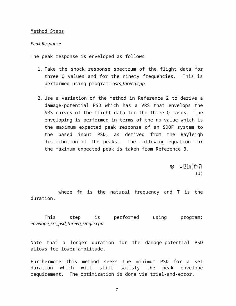
The comparisons in Figures A-3 through A-5 show that the damage potential PSD in Figure A-2 envelops the corresponding SRS curves in Figure A-1 in terms of peak response.
9

0.1
1
10
100
10 100 1000 2000
Damage PotentialFlight Data
NATURAL FREQUENCY (Hz)
PE
AK
AC
CE
L (G
)
RESPONSE SPECTRA Q = 25
Figure A-4.
0.1
1
10
100
10 100 1000 2000
Damage PotentialFlight Data
NATURAL FREQUENCY (Hz)
PE
AK
AC
CE
L (G
)
RESPONSE SPECTRA Q = 10
Figure A-5.
10

-20
-10
0
10
20
0 5 10 15 20 25 30 35 40 45 50 55 60
TIME (SEC)
AC
CE
L (G
)
SYNTHESIZED TIME HISTORY FOR DAMAGE POTENTIAL PSD OVERALL LEVEL = 3.3 GRMS
Figure A-6.
0.0001
0.001
0.01
0.1
10 100 1000 2000
SynthesisDamage Potential
FREQUENCY (Hz)
AC
CE
L (G
2 /Hz)
POWER SPECTRAL DENSITY OVERALL LEVEL = 3.3 GRMS
Figure A-7.
A time history is synthesized for the Damage Potential PSD.
11

1
10
100
1000
10 100 1000 2000
Damage SynthesisFlight Data
NATURAL FREQUENCY (Hz)
PE
AK
AC
CE
L (G
)
SHOCK RESPONSE SPECTRA Q=50
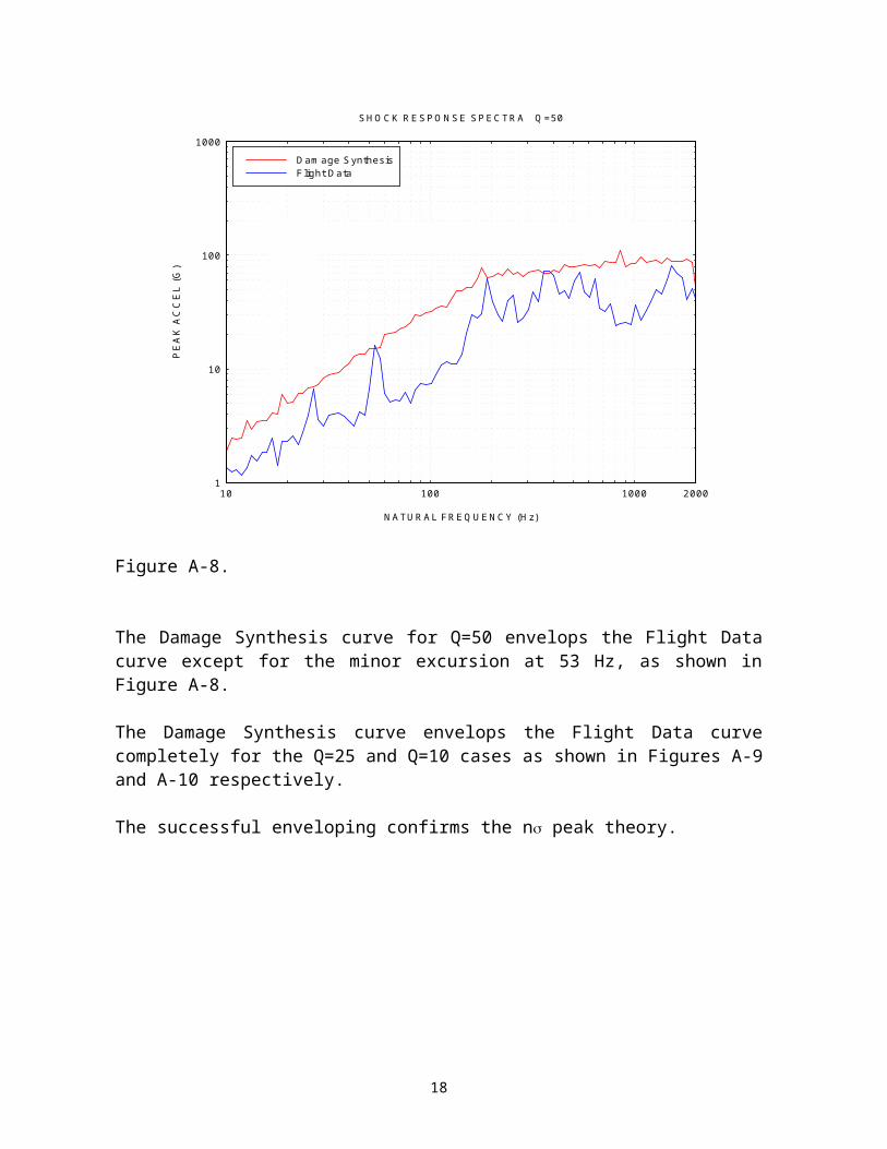
Figure A-8.
The Damage Synthesis curve for Q=50 envelops the Flight Data curve except for the minor excursion at 53 Hz, as shown in Figure A-8.
The Damage Synthesis curve envelops the Flight Data curve completely for the Q=25 and Q=10 cases as shown in Figures A-9 and A-10 respectively.
The successful enveloping confirms the n peak theory.
12

1
10
100
1000
10 100 1000 2000
Damage SynthesisFlight Data
NATURAL FREQUENCY (Hz)
PE
AK
AC
CE
L (G
)
SHOCK RESPONSE SPECTRA Q=25
Figure A-9.
1
10
100
1000
10 100 1000 2000
Damage SynthesisFlight Data
NATURAL FREQUENCY (Hz)
PE
AK
AC
CE
L (G
)
SHOCK RESPONSE SPECTRA Q=10
Figure A-10.
13

-100
-90
-80
-70
-60
-50
-40
-30
-20
-10
0
10
20
30
-5 0 5 10 15 20 25 30 35 40 45 50 55 60 65 70-40
-30
-20
-10
0
10
20
30
40
50
60
70
80
90
Damage Potential Synthesis
Flight Data
AC
CE
L (G
)
AC
CE
L (G
)
SDOF RESPONSE fn = 189 Hz Q=10
Figure A-11.
The respective Flight Data and Damage Potential Responses for a particular SDOF system are shown in Figure A-11.
14
-100
-90
-80
-70
-60
-50
-40
-30
-20
-10
0
10
20
30
-5 0 5 10 15 20 25 30 35 40 45 50 55 60 65 70-40
-30
-20
-10
0
10
20
30
40
50
60
70
80
90
Damage Potential Synthesis
Flight Data
AC
CE
L (G
)
AC
CE
L (G
)
SDOF RESPONSE fn = 280 Hz Q=10
Figure A-12.
The respective Flight Data and Damage Potential Responses for another SDOF system are shown in Figure A-12.
15

0.00001
0.0001
0.001
0.01
0.1
10 100 1000300 2000
FREQUENCY (Hz)
AC
CE
L (G
2 /Hz)
PSD SDOF (fn=280 Hz, Q=10) RESPONSE TO FLIGHT DATAOVERALL LEVEL = 1.1 GRMS
Figure A-13.
The highest spectral peak occurs at 280 Hz which is the resonant response.
But the response energy also occurs at other frequencies such as 190 Hz.
Thus non-resonant responses should be included in fatigue analysis. This can be done via rainflow cycle counting.
16

102
105
108
1011
1014
1017
10 100 1000 2000
Damage SynthesisFlight Data
NATURAL FREQUENCY (Hz)
FATI
GU
E D
AM
AG
E D
FATIGUE DAMAGE Q=50 b=6.4
Figure A-14.
102
105
108
1011
1014
1017
10 100 1000 2000
Damage SynthesisFlight Data
NATURAL FREQUENCY (Hz)
FATI
GU
E D
AM
AG
E D
FATIGUE DAMAGE Q=25 b=6.4
Figure A-15.
17
102
105
108
1011
1014
1017
10 100 1000 2000
Damage SynthesisFlight Data
NATURAL FREQUENCY (Hz)
FATI
GU
E D
AM
AG
E D
FATIGUE DAMAGE Q=10 b=6.4
Figure A-16.
102
104
106
108
1010
1012
10 100 1000 2000
Damage SynthesisFlight Data
NATURAL FREQUENCY (Hz)
FATI
GU
E D
AM
AG
E D
FATIGUE DAMAGE Q=50 b=4
Figure A-17.
18

101
103
105
107
109
1011
10 100 1000 2000
Damage SynthesisFlight Data
NATURAL FREQUENCY (Hz)
FATI
GU
E D
AM
AG
E D
FATIGUE DAMAGE Q=25 b=4
Figure A-18.
101
103
105
107
109
1011
10 100 1000 2000
Damage SynthesisFlight Data
NATURAL FREQUENCY (Hz)
FATI
GU
E D
AM
AG
E D
FATIGUE DAMAGE Q=10 b=4
Figure A-19.
19

The previous figures have shown that the Damage Potential PSD in Figure A-2 envelops the flight accelerometer data in terms of peak response and fatigue damage.
The Flight Data had a minor excursion above the Damage Potential at 53 Hz, as shown in the SRS Q=50 comparison in Figure A-8. But this excursion can probably be ignored given that most avionics circuit board fundamental frequencies are above 200 Hz. Otherwise the Damage Potential PSD could be slightly increased at 53 Hz to render the envelope complete.
As an aside, consider a maximax approach where the flight data is divided into 2.5-second segments. A PSD is calculated for each segment. Then a maximum envelope PSD is taken, as shown in Figure A-20. The frequency resolution is one-twelfth octave.
The Damage Potential PSD is superimposed in Figure A-20 for comparison. The Damage Potential PSD has a higher overall GRMS level, but the Maximax curve has higher G^2/Hz levels at a few frequencies.
The VRS curves for the two PSDs are shown in Figure A-21. The Maximax VRS exceeds the Damage Potential VRS at several natural frequencies. In a roundabout way, this shows that the Maximax curve is unnecessarily conservative, at least at the exceedance frequencies.
Further analysis would be needed to determine whether the Maximax PSD envelops the flight data in terms of fatigue.
20

0.0001
0.001
0.01
0.1
10 100 1000300 2000
Damage Potential 3.3 GRMSMaximax 2.0 GRMS
FREQUENCY (Hz)
AC
CE
L (G
2 /Hz)
PSD COMPARISON
Figure A-20.
0.1
1
10
10 100 1000300 2000
Damage PotentialMaximax
NATURAL FREQUENCY (Hz)
AC
CE
L (G
RM
S)
VRS Q=10 COMPARISON
Figure A-21.
21

APPENDIX B
Shock Response Spectrum Model
The shock response spectrum is a calculated function based on the acceleration time history. It applies an acceleration time history as a base excitation to an array of single-degree-of-freedom (SDOF) systems, as shown in Figure B-1. Note that each system is assumed to have no mass-loading effect on the base input.
Figure B-1. Shock Response Spectrum Model
Y is the common base input for each system. The double-dot denotes acceleration.
Each system is indexed with the letter i.
X i is the absolute peak response
M i is the mass
C i is the damping coefficient
K i is the stiffness.
fni is the natural frequency
The damping of each system is fixed at some Q value. The natural frequency is an independent variable.
The response calculation is performed for a number of independent SDOF systems, each with a unique natural frequency.
22