the gee procedure - sas support · covariance matrix, and the corrw option requests the working...
TRANSCRIPT

SAS/STAT® 14.1 User’s GuideThe GEE Procedure

This document is an individual chapter from SAS/STAT® 14.1 User’s Guide.
The correct bibliographic citation for this manual is as follows: SAS Institute Inc. 2015. SAS/STAT® 14.1 User’s Guide. Cary, NC:SAS Institute Inc.
SAS/STAT® 14.1 User’s Guide
Copyright © 2015, SAS Institute Inc., Cary, NC, USA
All Rights Reserved. Produced in the United States of America.
For a hard-copy book: No part of this publication may be reproduced, stored in a retrieval system, or transmitted, in any form or byany means, electronic, mechanical, photocopying, or otherwise, without the prior written permission of the publisher, SAS InstituteInc.
For a web download or e-book: Your use of this publication shall be governed by the terms established by the vendor at the timeyou acquire this publication.
The scanning, uploading, and distribution of this book via the Internet or any other means without the permission of the publisher isillegal and punishable by law. Please purchase only authorized electronic editions and do not participate in or encourage electronicpiracy of copyrighted materials. Your support of others’ rights is appreciated.
U.S. Government License Rights; Restricted Rights: The Software and its documentation is commercial computer softwaredeveloped at private expense and is provided with RESTRICTED RIGHTS to the United States Government. Use, duplication, ordisclosure of the Software by the United States Government is subject to the license terms of this Agreement pursuant to, asapplicable, FAR 12.212, DFAR 227.7202-1(a), DFAR 227.7202-3(a), and DFAR 227.7202-4, and, to the extent required under U.S.federal law, the minimum restricted rights as set out in FAR 52.227-19 (DEC 2007). If FAR 52.227-19 is applicable, this provisionserves as notice under clause (c) thereof and no other notice is required to be affixed to the Software or documentation. TheGovernment’s rights in Software and documentation shall be only those set forth in this Agreement.
SAS Institute Inc., SAS Campus Drive, Cary, NC 27513-2414
July 2015
SAS® and all other SAS Institute Inc. product or service names are registered trademarks or trademarks of SAS Institute Inc. in theUSA and other countries. ® indicates USA registration.
Other brand and product names are trademarks of their respective companies.

Chapter 43
The GEE Procedure
ContentsOverview: GEE Procedure . . . . . . . . . . . . . . . . . . . . . . . . . . . . . . . . . . . 2929Getting Started . . . . . . . . . . . . . . . . . . . . . . . . . . . . . . . . . . . . . . . . . 2930Syntax: GEE Procedure . . . . . . . . . . . . . . . . . . . . . . . . . . . . . . . . . . . . 2933
PROC GEE Statement . . . . . . . . . . . . . . . . . . . . . . . . . . . . . . . . . . 2934BY Statement . . . . . . . . . . . . . . . . . . . . . . . . . . . . . . . . . . . . . . 2935CLASS Statement . . . . . . . . . . . . . . . . . . . . . . . . . . . . . . . . . . . . 2935ESTIMATE Statement . . . . . . . . . . . . . . . . . . . . . . . . . . . . . . . . . . 2936FREQ Statement . . . . . . . . . . . . . . . . . . . . . . . . . . . . . . . . . . . . . 2937LSMEANS Statement . . . . . . . . . . . . . . . . . . . . . . . . . . . . . . . . . . 2938MISSMODEL Statement . . . . . . . . . . . . . . . . . . . . . . . . . . . . . . . . 2939MODEL Statement . . . . . . . . . . . . . . . . . . . . . . . . . . . . . . . . . . . . 2939OUTPUT Statement . . . . . . . . . . . . . . . . . . . . . . . . . . . . . . . . . . . 2942REPEATED Statement . . . . . . . . . . . . . . . . . . . . . . . . . . . . . . . . . . 2944WEIGHT Statement . . . . . . . . . . . . . . . . . . . . . . . . . . . . . . . . . . . 2948
Details: GEE Procedure . . . . . . . . . . . . . . . . . . . . . . . . . . . . . . . . . . . . 2948Generalized Estimating Equations . . . . . . . . . . . . . . . . . . . . . . . . . . . . 2948Alternating Logistic Regression . . . . . . . . . . . . . . . . . . . . . . . . . . . . . 2951Weighted Generalized Estimating Equations under the MAR Assumption . . . . . . . 2955ODS Table Names . . . . . . . . . . . . . . . . . . . . . . . . . . . . . . . . . . . . 2959ODS Graphics . . . . . . . . . . . . . . . . . . . . . . . . . . . . . . . . . . . . . . 2960
Examples: GEE Procedure . . . . . . . . . . . . . . . . . . . . . . . . . . . . . . . . . . . 2961Example 43.1: Comparison of the Marginal and Random Effect Models for Binary Data 2961Example 43.2: Log-Linear Model for Count Data . . . . . . . . . . . . . . . . . . . . 2964Example 43.3: Weighted GEE for Longitudinal Data That Have Missing Values . . . 2968Example 43.4: GEE for Binary Data with Logit Link Function . . . . . . . . . . . . . 2972Example 43.5: Alternating Logistic Regression for Ordinal Multinomial Data . . . . . 2975Example 43.6: GEE for Nominal Multinomial Data . . . . . . . . . . . . . . . . . . . 2978
References . . . . . . . . . . . . . . . . . . . . . . . . . . . . . . . . . . . . . . . . . . . 2980
Overview: GEE ProcedureThe GEE procedure implements the generalized estimating equations (GEE) approach (Liang and Zeger1986), which extends the generalized linear model to handle longitudinal data (Stokes, Davis, and Koch 2012;

2930 F Chapter 43: The GEE Procedure
Fitzmaurice, Laird, and Ware 2011; Diggle et al. 2002). For longitudinal studies, missing data are common,and they can be caused by dropouts or skipped visits. If missing responses depend on previous responses,the usual GEE approach can lead to biased estimates. So the GEE procedure also implements the weightedGEE method to handle missing responses that are caused by dropouts in longitudinal studies (Robins andRotnitzky 1995; Preisser, Lohman, and Rathouz 2002). The GEE procedure in SAS/STAT 14.1 does notsupport the weighted GEE method for the multinomial distribution for polytomous responses.
The GEE method fits a marginal model to longitudinal data. The regression parameters in the marginal modelare interpreted as population-averaged. For more information about the GEE method, see Fitzmaurice, Laird,and Ware (2011); Hardin and Hilbe (2003); Diggle et al. (2002); Lipsitz et al. (1994).
The GEE procedure compares most closely to the GENMOD procedure in SAS/STAT software. Bothprocedures implement the standard generalized estimating equation approach for longitudinal data; thisapproach is appropriate for complete data or when data are missing completely at random (MCAR). Whenthe data are missing at random (MAR), the weighted GEE method produces valid inference. Molenberghsand Kenward (2007); Fitzmaurice, Laird, and Ware (2011); Mallinckrodt (2013); O’Kelly and Ratitch (2014)describe the weighted GEE method.
The GEE procedure includes alternating logistic regression (ALR) analysis for binary and ordinal multinomialresponses. In ordinary GEEs, the association between pairs of responses are modeled with correlations. TheALR approach provides an alternative by using the log odds ratio to model the association between pairs.For more information about the log odds ratio and the ALR method, see the section “Alternating LogisticRegression” on page 2951. For binary responses the ALR algorithm of Carey, Zeger, and Diggle (1993) isimplemented in both the GEE and GENMOD procedures. The GEE procedure also implements the ALRalgorithm of Heagerty and Zeger (1996), which extends the ALR approach to ordinal multinomial responses.An ordinary GEE with the independent working correlation structure is also available for both nominal andordinal multinomial data.
Getting StartedThis section illustrates some of the basic features of the GEE procedure by analyzing longitudinal data fromStokes, Davis, and Koch (2012).
In this study, researchers followed 25 children at ages 8, 9, 10, and 11 years. The goal of this study is toinvestigate the health effects of air pollution on children. The binary response is the wheezing status of thechildren at four different ages. The explanatory variables are age, city, and passive smoking index (withvalues 0, 1, 2) that represented the degree of smoking in the home. The responses for individual children areassumed to be equally correlated, implying an exchangeable correlation structure.
The following statements create the data set Children:
data Children;input ID City$ @@;do i=1 to 4;
input Age Smoke Symptom @@;output;
end;

Getting Started F 2931
datalines;1 steelcity 8 0 1 9 0 1 10 0 1 11 0 02 steelcity 8 2 1 9 2 1 10 2 1 11 1 03 steelcity 8 2 1 9 2 0 10 1 0 11 0 04 greenhills 8 0 0 9 1 1 10 1 1 11 0 05 steelcity 8 0 0 9 1 0 10 1 0 11 1 06 greenhills 8 0 1 9 0 0 10 0 0 11 0 17 steelcity 8 1 1 9 1 1 10 0 1 11 0 08 greenhills 8 1 0 9 1 0 10 1 0 11 2 09 greenhills 8 2 1 9 2 0 10 1 1 11 1 0
10 steelcity 8 0 0 9 0 0 10 0 0 11 1 011 steelcity 8 1 1 9 0 0 10 0 0 11 0 112 greenhills 8 0 0 9 0 0 10 0 0 11 0 013 steelcity 8 2 1 9 2 1 10 1 0 11 0 114 greenhills 8 0 1 9 0 1 10 0 0 11 0 015 steelcity 8 2 0 9 0 0 10 0 0 11 2 116 greenhills 8 1 0 9 1 0 10 0 0 11 1 017 greenhills 8 0 0 9 0 1 10 0 1 11 1 118 steelcity 8 1 1 9 2 1 10 0 0 11 1 019 steelcity 8 2 1 9 1 0 10 0 1 11 0 020 greenhills 8 0 0 9 0 1 10 0 1 11 0 021 steelcity 8 1 0 9 1 0 10 1 0 11 2 122 greenhills 8 0 1 9 0 1 10 0 0 11 0 023 steelcity 8 1 1 9 1 0 10 0 1 11 0 024 greenhills 8 1 0 9 1 1 10 1 1 11 2 125 greenhills 8 0 1 9 0 0 10 0 0 11 0 0;
The following statements fit the model by the GEE method:
proc gee data=Children descending;class ID City;model Symptom = City Age Smoke / dist=bin link=logit;repeated subject=ID / type=exch covb corrw;
run;
Both the MODEL statement and the REPEATED statement are required.
The DIST=BIN and LINK=LOGIT options in the MODEL statement request a logistic regression with thevariable Symptom as the response and City, Age, and Smoke as explanatory variables.
The REPEATED statement specifies the correlation structure and requests various tables in the output. TheSUBJECT=ID option requests that individual subjects be identified in the input data set by the variable ID,which must be listed in the CLASS statement. Measurements of individual subjects at ages 8, 9, 10, and 11are in the proper order in the data set, so the WITHIN= option is not required. The TYPE=EXCH optionspecifies an exchangeable working correlation structure, the COVB option requests the parameter estimatecovariance matrix, and the CORRW option requests the working correlation matrix.
Figure 43.1 shows the “Model Information” table, which provides information about the specified logisticregression model and the input data set.

2932 F Chapter 43: The GEE Procedure
Figure 43.1 Model Information
The GEE ProcedureThe GEE Procedure
Model Information
Data Set WORK.CHILDREN
Distribution Binomial
Link Function Logit
Dependent Variable Symptom
Figure 43.2 displays general information about the GEE analysis. Each subject has four measurements.
Figure 43.2 GEE Model Information
GEE Model Information
Correlation Structure Exchangeable
Subject Effect ID (25 levels)
Number of Clusters 25
Correlation Matrix Dimension 4
Maximum Cluster Size 4
Minimum Cluster Size 4
Figure 43.3 displays the model-based and empirical covariance matrices of the parameter estimates.
Figure 43.3 Covariance Matrices of Parameter Estimates
Covariance Matrix (Model-Based)
Prm1 Prm2 Prm4 Prm5
Prm1 3.26069 -0.16313 -0.32274 -0.12257
Prm2 -0.16313 0.24015 0.002520 0.03422
Prm4 -0.32274 0.002520 0.03379 0.004471
Prm5 -0.12257 0.03422 0.004471 0.09533
Covariance Matrix (Empirical)
Prm1 Prm2 Prm4 Prm5
Prm1 4.09770 -0.55261 -0.37280 -0.29397
Prm2 -0.55261 0.29538 0.03719 0.09143
Prm4 -0.37280 0.03719 0.03550 0.02064
Prm5 -0.29397 0.09143 0.02064 0.07957
The exchangeable working correlation matrix is displayed in Figure 43.4.
Figure 43.4 Working Correlation Matrix
Working Correlation Matrix
Obs 1 Obs 2 Obs 3 Obs 4
Obs 1 1.0000 0.0883 0.0883 0.0883
Obs 2 0.0883 1.0000 0.0883 0.0883
Obs 3 0.0883 0.0883 1.0000 0.0883
Obs 4 0.0883 0.0883 0.0883 1.0000

Syntax: GEE Procedure F 2933
The parameter estimates table, shown in Figure 43.5, contains parameter estimates, standard errors, confidenceintervals, Z scores, and p-values for the parameter estimates. Empirical standard error estimates are used inthis table. You can create a table that uses model-based standard errors by specifying the MODELSE optionin the REPEATED statement. The results indicate that smoking exposure is significant with a p-value of0.0211, Age is marginally influential with a p-value of 0.0893, and City does not influence wheezing. Theparameter estimate for Age is –0.3201, which indicates that the odds ratio of wheezing for the children at thehigher age group compared to those in the lower age group is e�0:3201 D 0:726.
Figure 43.5 GEE Parameter Estimates Table
Parameter Estimates for Response Model
with Empirical Standard Error Estimates
Parameter EstimateStandard
Error
95%Confidence
Limits Z Pr > |Z|
Intercept 2.2615 2.0243 -1.7060 6.2290 1.12 0.2639
City greenhil 0.0418 0.5435 -1.0234 1.1070 0.08 0.9387
City steelcit 0.0000 0.0000 0.0000 0.0000 . .
Age -0.3201 0.1884 -0.6894 0.0492 -1.70 0.0893
Smoke 0.6506 0.2821 0.0978 1.2035 2.31 0.0211
Goodness-of-fit criteria for the model are displayed in Figure 43.6. For more information about the quasi-likelihood information criterion (QIC), see the section “Quasi-likelihood Information Criterion” on page 2950.
Figure 43.6 Model Fit Criteria
GEE FitCriteria
QIC 137.1373
QICu 136.2173
Syntax: GEE ProcedureThe following statements are available in the GEE procedure. Items within < > are optional.
PROC GEE < options > ;BY variables ;CLASS variable < (options) > . . . < variable < (options) > > < / options > ;ESTIMATE < 'label ' > estimate-specification < / options > ;FREQ | FREQUENCY variable ;LSMEANS < model-effects > < / options > ;MISSMODEL < effects > < / options > ;MODEL response = < effects > < / options > ;OUTPUT < OUT=SAS-data-set > < keyword=name . . . keyword=name > ;REPEATED SUBJECT=subject-effect < / options > ;WEIGHT variable ;

2934 F Chapter 43: The GEE Procedure
The syntax of the GEE procedure compares most closely to that of the GENMOD procedures. The PROCGEE, MODEL, and REPEATED statements are required. All other statements can appear only once. Thefollowing sections describe the PROC GEE statement and then describe the other statements in alphabeticalorder.
PROC GEE StatementPROC GEE < options > ;
The PROC GEE statement invokes the GEE procedure. Table 43.1 summarizes the options available in thePROC GEE statement.
Table 43.1 PROC GEE Statement Options
Option Description
DATA= Specifies the input data setDESCENDING Sorts the response variable in the reverse of the default orderNAMELEN= Specifies the length of effect namesORDER= Specifies the sort order of CLASS variablePLOTS Controls the plots that are produced through ODS Graphics
You can specify the following options.
DATA=SAS-data-setspecifies the SAS data set that contains the data to be analyzed. If you omit the DATA= option, PROCGEE uses the most recently created SAS data set.
DESCENDING
DESCEND
DESCrequests that the levels of the response variable for the binomial model that uses a single-variableresponse syntax be sorted in the reverse of the default order.
NAMELEN=numberspecifies the length to which long effect names are shortened. The default and minimum value is 20.
PLOTS < = plot-request >controls the plots produced through ODS Graphics. For example:
proc gee plots=histogram;model y=x1;
run;
For more information about enabling and disabling ODS Graphics, see the section “Enabling andDisabling ODS Graphics” on page 609 in Chapter 21, “Statistical Graphics Using ODS.”
You can specify the following plot-requests:

BY Statement F 2935
ALLrequests that all default plots be produced.
HISTOGRAMcreates a histogram for the predicted weights from the missingness model.
NONEsuppresses all plots.
BY StatementBY variables ;
You can specify a BY statement with PROC GEE to obtain separate analyses of observations in groups thatare defined by the BY variables. When a BY statement appears, the procedure expects the input data set to besorted in order of the BY variables. If you specify more than one BY statement, only the last one specified isused.
If your input data set is not sorted in ascending order, use one of the following alternatives:
� Sort the data by using the SORT procedure with a similar BY statement.
� Specify the NOTSORTED or DESCENDING option in the BY statement for the GEE procedure. TheNOTSORTED option does not mean that the data are unsorted but rather that the data are arrangedin groups (according to values of the BY variables) and that these groups are not necessarily inalphabetical or increasing numeric order.
� Create an index on the BY variables by using the DATASETS procedure (in Base SAS software).
For more information about BY-group processing, see the discussion in SAS Language Reference: Concepts.For more information about the DATASETS procedure, see the discussion in the Base SAS Procedures Guide.
CLASS StatementCLASS variables < / options > ;
The CLASS statement names the classification variables to be used in the analysis. If the CLASS statementis used, it must appear before the MODEL statement.
Classification variables can be either character or numeric. CLASS levels are determined from the formattedvalues of the variables. Thus, you can use formats to group values into levels. For more information, seethe discussion of the FORMAT procedure in the Base SAS Procedures Guide and the discussions of theFORMAT statement and SAS formats in SAS Formats and Informats: Reference.
You can specify the following options for classification variables:
DESCENDINGDESC
reverses the sort order of the classification variable. If you specify both the DESCENDING andORDER= options, PROC GEE orders the categories according to the ORDER= option and thenreverses that order.

2936 F Chapter 43: The GEE Procedure
ORDER=order-typespecifies the sort order for the categories of categorical variables. This ordering determines whichparameters in the model correspond to each level in the data. When the default ORDER=FORMATTEDis in effect for numeric variables for which you have supplied no explicit format, the levels are orderedby their internal values. Table 43.2 shows how PROC GEE interprets values of the ORDER= option.
Table 43.2 Sort Order for Categorical Variables
order-type Levels Sorted By
DATA Order of appearance in the input data setFORMATTED External formatted value, except for numeric variables that have no
explicit format, which are sorted by their unformatted (internal) valueFREQ Descending frequency count; levels that have the most observations
come first in the orderFREQDATA Order of descending frequency count, and within counts by order of
appearance in the input data set when counts are tiedFREQFORMATTED Order of descending frequency count, and within counts by formatted
value (as above) when counts are tiedFREQINTERNAL Order of descending frequency count, and within counts by unformat-
ted value when counts are tiedINTERNAL Unformatted value
For the FORMATTED and INTERNAL values, the sort order is machine-dependent. If you specifythe ORDER= option in the MODEL statement and the ORDER= option in the CLASS statement, theformer takes precedence.
For more information about sort order, see the chapter on the SORT procedure in the Base SASProcedures Guide and the discussion of BY-group processing in SAS Language Reference: Concepts.
ESTIMATE StatementESTIMATE < 'label ' > estimate-specification < (divisor=n) >
< , . . . < 'label ' > estimate-specification < (divisor=n) > >< / options > ;
The ESTIMATE statement provides a mechanism for obtaining custom hypothesis tests. Estimates areformed as linear estimable functions of the form Lˇ. You can perform hypothesis tests for the estimablefunctions, construct confidence limits, and obtain specific nonlinear transformations.
Table 43.3 summarizes the options available in the ESTIMATE statement.
Table 43.3 ESTIMATE Statement Options
Option Description
Construction and Computation of Estimable FunctionsDIVISOR= Specifies a list of values to divide the coefficients

FREQ Statement F 2937
Table 43.3 continued
Option Description
NOFILL Suppresses the automatic fill-in of coefficients for higher-ordereffects
SINGULAR= Tunes the estimability checking difference
Degrees of Freedom and p-valuesADJUST= Determines the method for multiple comparison adjustment of
estimatesALPHA=˛ Determines the confidence level (1 � ˛)LOWER Performs one-sided, lower-tailed inferenceSTEPDOWN Adjusts multiplicity-corrected p-values further in a step-down
fashionTESTVALUE= Specifies values under the null hypothesis for testsUPPER Performs one-sided, upper-tailed inference
Statistical OutputCL Constructs confidence limitsCORR Displays the correlation matrix of estimatesCOV Displays the covariance matrix of estimatesE Prints the L matrixJOINT Produces a joint F or chi-square test for the estimable functionsPLOTS= Requests ODS statistical graphics if the analysis is sampling-basedSEED= Specifies the seed for computations that depend on random
numbers
Generalized Linear ModelingCATEGORY= Specifies how to construct estimable functions with multinomial
dataEXP Exponentiates and displays estimatesILINK Computes and displays estimates and standard errors on the inverse
linked scale
For details about the syntax of the ESTIMATE statement, see the section “ESTIMATE Statement” onpage 448 in Chapter 19, “Shared Concepts and Topics.”
FREQ StatementFREQ variable ;
FREQUENCY variable ;
The variable in the FREQ statement identifies a variable in the input data set that contains the frequency ofoccurrence of each observation. PROC GEE treats each observation as if it appeared n times, where n is thevalue of the FREQ variable for the observation. If the frequency value is not an integer, it is truncated to an
2938 F Chapter 43: The GEE Procedure
integer. If it is less than 1 or missing, the observation is not used. The frequencies must be the same for allobservations within each subject.
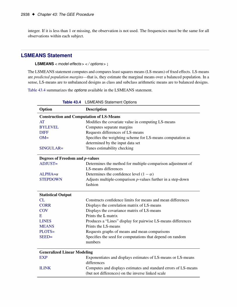
LSMEANS StatementLSMEANS < model-effects > < / options > ;
The LSMEANS statement computes and compares least squares means (LS-means) of fixed effects. LS-meansare predicted population margins—that is, they estimate the marginal means over a balanced population. In asense, LS-means are to unbalanced designs as class and subclass arithmetic means are to balanced designs.
Table 43.4 summarizes the options available in the LSMEANS statement.
Table 43.4 LSMEANS Statement Options
Option Description
Construction and Computation of LS-MeansAT Modifies the covariate value in computing LS-meansBYLEVEL Computes separate marginsDIFF Requests differences of LS-meansOM= Specifies the weighting scheme for LS-means computation as
determined by the input data setSINGULAR= Tunes estimability checking
Degrees of Freedom and p-valuesADJUST= Determines the method for multiple-comparison adjustment of
LS-means differencesALPHA=˛ Determines the confidence level (1 � ˛)STEPDOWN Adjusts multiple-comparison p-values further in a step-down
fashion
Statistical OutputCL Constructs confidence limits for means and mean differencesCORR Displays the correlation matrix of LS-meansCOV Displays the covariance matrix of LS-meansE Prints the L matrixLINES Produces a “Lines” display for pairwise LS-means differencesMEANS Prints the LS-meansPLOTS= Requests graphs of means and mean comparisonsSEED= Specifies the seed for computations that depend on random
numbers
Generalized Linear ModelingEXP Exponentiates and displays estimates of LS-means or LS-means
differencesILINK Computes and displays estimates and standard errors of LS-means
(but not differences) on the inverse linked scale

MISSMODEL Statement F 2939
Table 43.4 continued
Option Description
ODDSRATIO Reports (simple) differences of least squares means in terms ofodds ratios if permitted by the link function
For details about the syntax of the LSMEANS statement, see the section “LSMEANS Statement” on page 464in Chapter 19, “Shared Concepts and Topics.”
MISSMODEL StatementMISSMODEL effects < / options > ;
The MISSMODEL statement requests a weighted GEE analysis. It specifies a logistic regression that isused to estimate the weights under the MAR assumption. If the pattern of missing data is intermittent (notdropout), the GEE procedure terminates and does not perform an analysis.
You can use the same effects or different effects in the MODEL and MISSMODEL statements. Explanatoryvariables can be continuous or classification variables. Classification variables can be character or numeric.Explanatory variables that represent nominal (classification) data must be declared in a CLASS statement.Interactions between variables can also be included as effects. Columns of the design matrix are automaticallygenerated for classification variables and interactions. The syntax for effects is the same as for the GLMprocedure. For more information, see the section “Specification of Effects” on page 3593 in Chapter 46,“The GLM Procedure.”
You can specify the following options after a slash (/).
MAXWEIGHT=numbertruncates the predicted weights from the missingness model if they are larger than number , wherenumber � 1.
TYPE=OBSLEVEL | SUBLEVELspecifies the type of weighted GEE method. You can specify the following values:
OBSLEVEL specifies the observation-level weighted GEE method.
SUBLEVEL specifies the subject-level weighted GEE method.
By default, TYPE=OBSLEVEL.
MODEL StatementMODEL response = < effects > < / options > ;
MODEL events/trials = < effects > < / options > ;
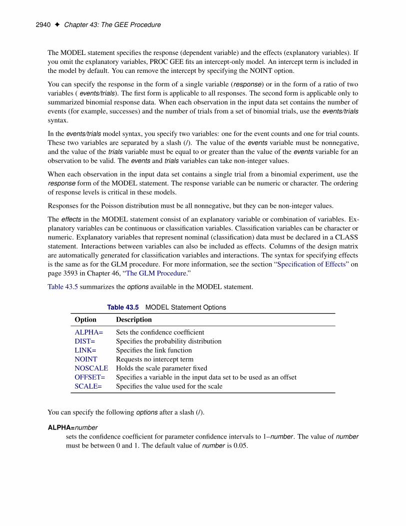
2940 F Chapter 43: The GEE Procedure
The MODEL statement specifies the response (dependent variable) and the effects (explanatory variables). Ifyou omit the explanatory variables, PROC GEE fits an intercept-only model. An intercept term is included inthe model by default. You can remove the intercept by specifying the NOINT option.
You can specify the response in the form of a single variable (response) or in the form of a ratio of twovariables ( events/trials). The first form is applicable to all responses. The second form is applicable only tosummarized binomial response data. When each observation in the input data set contains the number ofevents (for example, successes) and the number of trials from a set of binomial trials, use the events/trialssyntax.
In the events/trials model syntax, you specify two variables: one for the event counts and one for trial counts.These two variables are separated by a slash (/). The value of the events variable must be nonnegative,and the value of the trials variable must be equal to or greater than the value of the events variable for anobservation to be valid. The events and trials variables can take non-integer values.
When each observation in the input data set contains a single trial from a binomial experiment, use theresponse form of the MODEL statement. The response variable can be numeric or character. The orderingof response levels is critical in these models.
Responses for the Poisson distribution must be all nonnegative, but they can be non-integer values.
The effects in the MODEL statement consist of an explanatory variable or combination of variables. Ex-planatory variables can be continuous or classification variables. Classification variables can be character ornumeric. Explanatory variables that represent nominal (classification) data must be declared in a CLASSstatement. Interactions between variables can also be included as effects. Columns of the design matrixare automatically generated for classification variables and interactions. The syntax for specifying effectsis the same as for the GLM procedure. For more information, see the section “Specification of Effects” onpage 3593 in Chapter 46, “The GLM Procedure.”
Table 43.5 summarizes the options available in the MODEL statement.
Table 43.5 MODEL Statement Options
Option Description
ALPHA= Sets the confidence coefficientDIST= Specifies the probability distributionLINK= Specifies the link functionNOINT Requests no intercept termNOSCALE Holds the scale parameter fixedOFFSET= Specifies a variable in the input data set to be used as an offsetSCALE= Specifies the value used for the scale
You can specify the following options after a slash (/).
ALPHA=numbersets the confidence coefficient for parameter confidence intervals to 1–number . The value of numbermust be between 0 and 1. The default value of number is 0.05.

MODEL Statement F 2941
DIST=keyword
D=keyword
ERROR=keyword
ERR=keywordspecifies the built-in probability distribution to use in the model. If you specify the DIST= optionand you omit the LINK= option, a default link function is chosen as displayed in Table 43.6. If youspecify neither the DIST= option nor the LINK= option, then the GEE procedure defaults to the normaldistribution with the identity link function.
Table 43.6 Distributions and Default Link Functions
DIST= Distribution Default Link Function
BINOMIAL | BIN | B Binomial LogitGAMMA | GAM | G Gamma ReciprocalIGAUSSIAN | IG Inverse Gaussian Reciprocal squareMULTINOMIAL | MULT Multinomial Cumulative logitNEGBIN | NB Negative binomial LogNORMAL | NOR | N Normal IdentityPOISSON | POI | P Poisson Log
LINK=keywordspecifies the link function in the model. You can specify the keywords shown in Table 43.7.
Table 43.7 Built-In Link Functions of the GEE Procedure
LinkLINK= Function g.�/ D � D
CLOGLOG | CLL Complementary log-log log.� log.1 � �//CUMCLL | CCLL Cumulative complementary log-log log.� log.1 � �//CUMLOGIT| CLOGIT Cumulative logit log.�=.1 � �//CUMPROBIT | CPROBIT Cumulative probit ˆ�1.�/
GLOGIT Generalized logitIDENTITY | ID Identity �
LOG Log log.�/LOGIT Logit log.�=.1 � �//PROBIT Probit ˆ�1.�/
INVERSE | RECIPROCAL Reciprocal 1=�
POWERMINUS2 Power with exponent –2 1=�2
For the probit and cumulative probit links, ˆ�1.�/ denotes the quantile function of the standard normaldistribution. If you do not specify the LINK= option, then by default the canonical link function is usedif you specify the DIST= option. Otherwise, if you omit the DIST= option, the identity link function isused.

2942 F Chapter 43: The GEE Procedure
The cumulative link functions are appropriate only for the multinomial distribution with ordinalresponses, with cumulative probabilities indicated by � . The GLOGIT link function is appropriateonly for the multinomial distribution with nominal responses.
NOINTrequests that no intercept term be included in the model. An intercept is included unless this option isspecified.
NOSCALEholds the scale parameter fixed. Otherwise, for the normal, inverse Gaussian, and gamma distributions,the scale parameter is estimated by maximum likelihood. If you omit the SCALE= option, the scaleparameter is fixed at the value 1.
OFFSET=variablespecifies a variable in the input data set to be used as an offset variable. This variable cannot be aCLASS variable, the response variable, or any of the explanatory variables.
SCALE=numberSCALE=PEARSON | PPSCALESCALE=DEVIANCE | DDSCALE
specifies the value used for the scale parameter when the NOSCALE option is used. For the binomialand Poisson distributions, which have no free scale parameter, this can be used to specify an overdis-persed model. If the NOSCALE option is not specified, then number is used as an initial estimate ofthe scale parameter.
Specifying SCALE=PEARSON or SCALE=P is the same as specifying the PSCALE option. Thisfixes the scale parameter at the value 1 in the estimation procedure. After the parameter estimatesare determined, the exponential family dispersion parameter is assumed to be given by Pearson’schi-square statistic divided by the degrees of freedom, and all statistics such as standard errors areadjusted appropriately.
Specifying SCALE=DEVIANCE or SCALE=D is the same as specifying the DSCALE option. Thisfixes the scale parameter at a value of 1 in the estimation procedure.
OUTPUT StatementOUTPUT < OUT=SAS-data-set > < keyword=name . . . keyword=name > ;
The OUTPUT statement creates a new SAS data set that contains all the variables in the input data set and,optionally, the estimated linear predictors (XBETA) and their standard error estimates, predicted values ofthe mean, and confidence limits for predicted values.
If you use the multinomial distribution with one of the cumulative link functions for ordinal data, the dataset also contains variables named _ORDER_ and _LEVEL_ that indicate the levels of the ordinal responsevariable and the values of the variable in the input data set corresponding to the sorted levels. These variablesindicate that the predicted value for a given observation is the probability that the response variable is aslarge as the value of the _LEVEL_ variable. Residuals and other diagnostic statistics are not available for themultinomial distribution.

OUTPUT Statement F 2943
The estimated linear predictor, its standard error estimate, and the predicted values and their confidenceintervals are computed for all observations in which the explanatory variables are all nonmissing, even ifthe response is missing. By adding observations with missing response values to the input data set, you cancompute these statistics for new observations or for settings of the explanatory variables not present in thedata without affecting the model fit.
The following list explains specifications in the OUTPUT statement.
OUT=SAS-data-setspecifies the output data set. If you omit the OUT=option, the output data set is created and given adefault name that uses the DATAn convention.
keyword=namespecifies the statistics to be included in the output data set and names the new variables that contain thestatistics. Specify a keyword for each desired statistic (see the following list of keywords), an equalsign, and the name of the new variable or variables to contain the statistic.
Although you can use the OUTPUT statement without any keyword=name specifications, the outputdata set then contains only the original variables and, possibly, the variables Level and Value (if youuse the multinomial model with ordinal data).
The keywords allowed and the statistics they represent are as follows:
LOWER | L represents the lower confidence limit for the predicted value of the mean, or thelower confidence limit for the probability that the response is less than or equalto the value of Level or Value. The confidence coefficient is determined by theALPHA=number option in the MODEL statement as .1 � number/ � 100%. Thedefault confidence coefficient is 95%.
PREDICTED | PRED | PROB | P represents the predicted value of the mean of the response or thepredicted probability that the response variable is less than or equal to the valueof _LEVEL_ if the multinomial model for ordinal data is used (in other words,Pr.Y � _LEVEL_/, where Y is the response variable).
RESCHI represents the Pearson (chi) residual for identifying observations that are poorlyaccounted for by the model. This option is not available for the multinomialdistribution.
RESRAW represents the raw residual for identifying poorly fitted observations. This option isnot available for the multinomial distribution.
STDXBETA represents the standard error estimate of XBETA (see the XBETA keyword).
UPPER | U represents the upper confidence limit for the predicted value of the mean, or theupper confidence limit for the probability that the response is less than or equalto the value of Level or Value. The confidence coefficient is determined by theALPHA=number option in the MODEL statement as .1 � number/ � 100%. Thedefault confidence coefficient is 95%.
XBETA represents the estimate of the linear predictor x0iˇ for observation i, or ˛j Cx0iˇ, where j is the corresponding ordered value of the response variable for themultinomial model with ordinal data. If there is an offset, it is included in x0iˇ.

2944 F Chapter 43: The GEE Procedure
REPEATED StatementREPEATED SUBJECT=subject-effect < / options > ;
The REPEATED statement specifies the correlation structure of the responses for GEE model fitting. Inaddition, the REPEATED statement controls the iterative fitting algorithm and specifies optional output.
Table 43.8 summarizes the options available in the REPEATED statement.
Table 43.8 REPEATED Statement Options
Option Description
ALPHAINIT= Specifies initial values for log odds ratio regression parametersCONVERGE= Specifies the convergence criterion for GEE parameter estimationCORRB Displays the estimated correlation matrixCORRW Displays the estimated working correlation matrixCOVB Displays the estimated covariance matrixECORRB Displays the estimated empirical correlation matrixECOVB Displays the estimated empirical covariance matrixINITIAL= Specifies initial values of the regression parameters estimationINTERCEPT= Specifies an initial value of the interceptLOGOR= Specifies the use of alternating logistic regression and a model for the log
odds ratioMAXITER= Specifies the maximum number of iterationsMCORRB Displays the estimated model-based correlation matrixMCOVB Displays the estimated model-based covariance matrixMODELSE Displays a parameter estimates table with the model-based standard errorsSUBCLUSTER= Specifies a variable that defines subclustersSUBJECT= Identifies a different subject (cluster)TYPE= Specifies the working correlation matrix structureWITHIN= Specifies the order of measurements within subjectsZDATA= Specifies the full z matrixZROW= Specifies the rows of the z matrix
You must specify the SUBJECT= option:
SUBJECT=subject-effectidentifies subjects in the input data set. The subject-effect can be a single variable, an interaction effect,a nested effect, or a combination. Each distinct value (level) of the effect identifies a different subject(cluster). Responses from different subjects are assumed to be statistically independent, and responseswithin subjects are assumed to be correlated. You must specify a subject-effect , and you must listvariables that are used in defining the subject-effect in the CLASS statement.
You can also specify the following options after a slash (/) to control how the model is fit and what output isproduced:

REPEATED Statement F 2945
ALPHAINIT=numbersspecifies initial values for log odds ratio regression parameters if you specify the option LOGOR= fordata that have either binary or ordinal multinomial responses. The default value of numbers is 0.01.
CONVERGE=numberspecifies the convergence criterion for GEE parameter estimation. If the maximum absolute differencebetween regression parameter estimates is less than number on two successive iterations, convergenceis declared. If the absolute value of a regression parameter estimate is greater than 0.08, then theabsolute difference normalized by the regression parameter value is used instead of the absolutedifference. The default value of number is 0.0001.
CORRBdisplays the estimated regression parameter correlation matrix. Both model-based and empiricalcorrelations are displayed.
CORRWdisplays the estimated working correlation matrix. If you specify TYPE=EXCH for the exchangeableworking correlation structure, then the CORRW option is not needed to view the estimated correlation,because a table that contains the single estimated correlation is printed by default.
COVBdisplays the estimated regression parameter covariance matrix. Both model-based and empiricalcovariances are displayed.
ECORRBdisplays the estimated regression parameter empirical correlation matrix.
ECOVBdisplays the estimated regression parameter empirical covariance matrix.
INITIAL=numbersspecifies initial values of the regression parameters estimation, other than the intercept parameter, forGEE estimation. If you do not specify this option, then the estimated regression parameters (assumingindependence for all responses) are used for the initial values.
INTERCEPT=numberspecifies an initial value of the intercept regression parameter in the GEE model.
LOGOR=log-odds-ratio-structure-keywordspecifies the use of the alternating logistic regression (ALR) method and the regression model structurefor the log odds ratio. For data that have either a binary or ordinal multinomial response distribution,the ALR method uses the log odds ratio to model the association of the responses from subjects. Formore information about the ALR method and examples of specifying log odds ratio models, see thesection “Alternating Logistic Regression” on page 2951. You can specify the values that are shown inTable 43.9.

2946 F Chapter 43: The GEE Procedure
Table 43.9 Log Odds Ratio Regression Structures
Keyword Log Odds Ratio Regression Structure
EXCH ExchangeableFULLCLUST Fully parameterized clustersLOGORVAR(variable) Indicator variable for specifying block effectsNESTK k-nestedNEST1 1-nestedZFULL Fully specified z matrix specified in ZDATA= data setZREP Single cluster specification for replicated z matrix specified
in ZDATA= data setZREP(matrix) Single cluster specification for replicated z matrix
For ordinal multinomial data, only the exchangeable regression structure that is specified by LO-GOR=EXCH is supported. You should specify the option LOGOR= or TYPE=, but not both.
MAXITER=number
MAXIT=numberspecifies the maximum number of iterations allowed in the iterative GEE estimation process. Bydefault, MAXITER=50.
MCORRBdisplays the estimated regression parameter model-based correlation matrix.
MCOVBdisplays the estimated regression parameter model-based covariance matrix.
MODELSEdisplays a parameter estimates table that uses model-based standard errors for inference. By default, a“Parameter Estimates” table that is based on empirical standard errors is displayed.
SUBCLUSTER=variable
SUBCLUST=variablespecifies a variable that defines subclusters for the 1-nested or k-nested log odds ratio associationmodeling structures for data that have a binary response distribution. A 1-nested or k-nested modelingstructure is specified in the option LOGOR=, and variable must be listed in the CLASS statement. Fordefinitions of the 1-nested and k-nested modeling structures, see the section “Specifying Log OddsRatio Models” on page 2953.
TYPE=correlation-structure-keyword
CORR=correlation-structure-keywordspecifies the structure of the working correlation matrix that is used to model the correlation of theresponses from subjects for ordinary GEEs. You can specify the values that are shown in Table 43.10(for definitions of the correlation matrix types, see Table 43.11 in the section “Details: GEE Procedure”on page 2948).

REPEATED Statement F 2947
Table 43.10 Correlation Structure Types
Keyword Correlation Structure Type
AR | AR(1) Autoregressive(1)EXCH | CS ExchangeableIND IndependentMDEP(number ) m-dependent, where m = numberUNSTR | UN UnstructuredUSER(matrix) | FIXED(matrix) Fixed, user-specified correlation matrix
For example, the following option specifies a fixed 4 � 4 correlation matrix:
type=user( 1.0 0.9 0.8 0.60.9 1.0 0.9 0.80.8 0.9 1.0 0.90.6 0.8 0.9 1.0 )
By default, TYPE=IND. When you specify the alternating logistic regression method using the optionLOGOR= you should not specify TYPE=.
WITHINSUBJECT=within-subject-effect
WITHIN=within-subject-effectdefines an effect that specifies the order of measurements within subjects. Each distinct level of thewithin-subject-effect defines a different response from the same subject. If the data are in proper orderwithin each subject, you do not need to specify this option.
If some measurements do not appear in the data for some subjects, this option properly orders theexisting measurements and treats the omitted measurements as missing values.
If you do not specify the WITHIN= option for the standard GEE method, missing values are assumedto be the last values and are not used; the remaining observations are then ordered in the sequencein which they are provided in the input data set. If you do not specify the WITHIN= option for theweighted GEE method, the observations are assumed to be ordered in the sequence in which they areprovided in the input data set.
Variables that are used in defining the within-subject-effect must be listed in the CLASS statement.
ZDATA=SAS-data-setspecifies a SAS data set that contains either the full z matrix for log odds ratio association modeling fordata with binary responses or the z matrix for a single complete cluster to be replicated for all clusters.
ZROW=variable-listspecifies the variables in the ZDATA= data set that correspond to rows of the z matrix for log oddsratio association modeling for data with binary responses.

2948 F Chapter 43: The GEE Procedure
WEIGHT StatementWEIGHT variable ;
The WEIGHT statement identifies a variable in the input data set to be used as the exponential familydispersion parameter weight for each observation. The exponential family dispersion parameter is divided bythe WEIGHT variable value for each observation.
The WEIGHT variable value does not have to be an integer; if the value is less than or equal to 0 or if it ismissing, the corresponding observation is not used.
Details: GEE Procedure
Generalized Estimating EquationsThe marginal model is commonly used in analyzing longitudinal data when the population-averaged effect isof interest. To estimate the regression parameters in the marginal model, Liang and Zeger (1986) proposedthe generalized estimating equations method, which is widely used.
Suppose yij ; j D 1; : : : ; ni ; i D 1; : : : ; K, represent the jth response of the ith subject, which has a vectorof covariates xij . There are ni measurements on subject i, and the maximum number of measurements persubject is T.
Suppose the responses of the ith subject be Yi D Œyi1; : : : ; yini�0 with corresponding means �i D
Œ�i1; : : : ; �ini�0. For generalized linear models, the marginal mean �ij of the response yij is related
to a linear predictor through a link function g.�ij / D x0ijˇ, and the variance of yij depends on the meanthrough a variance function v.�ij /.
An estimate of the parameter ˇ in the marginal model can be obtained by solving the generalized estimatingequations,
S.ˇ/ DKXiD1
@�0i@ˇ
V�1i .Yi � �i .ˇ// D 0
where Vi is the working covariance matrix of Yi .
Only the mean and the covariance of Yi are required in the GEE method; a full specification of the jointdistribution of the correlated responses is not needed. This is particularly convenient because the jointdistribution for noncontinuous responses involves high-order associations and is complicated to specify.Moreover, the regression parameter estimates are consistent even when the working covariance is incorrectlyspecified. Because of these properties, the GEE method is popular in situations where the marginal effect isof interest and the responses are not continuous. However, the GEE approach can lead to biased estimateswhen missing responses depend on previous responses. The weighted GEE method, which is described inthe section “Weighted Generalized Estimating Equations under the MAR Assumption” on page 2955, canprovide unbiased estimates.

Generalized Estimating Equations F 2949
Working Correlation Matrix
Suppose Ri .˛/ is an ni � ni “working” correlation matrix that is fully specified by the vector of parameters˛. The covariance matrix of Yi is modeled as
Vi D �A12
i W� 1
2
i R.˛/W� 1
2
i A12
i
where Ai is an ni � ni diagonal matrix whose jth diagonal element is v.�ij / and Wi is an ni � ni diagonalmatrix whose jth diagonal is wij , where wij is a weight variable that is specified in the WEIGHT statement.If there is no WEIGHT statement, wij D 1 for all i and j. If Ri .˛/ is the true correlation matrix of Yi , thenVi is the true covariance matrix of Yi .
In practice, the working correlation matrix is usually unknown and must be estimated. It is estimated in theiterative fitting process by using the current value of the parameter vector ˇ to compute appropriate functionsof the Pearson residual:
eij Dyij � �ijpv.�ij /=wij
If you specify the working correlation matrix as R0 D I, which is the identity matrix, the GEE reduces to theindependence estimating equation.
Table 43.11 shows the working correlation structures that are supported by the GEE procedure and theestimators that are used to estimate the working correlations.
Table 43.11 Working Correlation Structures and Estimators
Working Correlation Structure Estimator
FixedCorr.Yij ; Yik/ D rjkwhere rjk is the jkth element of a constant,user-specified correlation matrix R0
The working correlation is not estimated in this case.
Independent
Corr.Yij ; Yik/ D�1 j D k
0 j ¤ kThe working correlation is not estimated in this case.
m-dependent
Corr.Yij ; Yi;jCt / D
8<:1 t D 0
˛t t D 1; 2; : : : ; m
0 t > m
O t D1
.Kt�p/�
PKiD1
Pj�ni�t
eij ei;jCt
Kt DPKiD1.ni � t /
Exchangeable
Corr.Yij ; Yik/ D�1 j D k
˛ j ¤ kO D
1.N��p/�
PKiD1
Pj<k eij eik
N � D 0:5PKiD1 ni .ni � 1/
Unstructured
Corr.Yij ; Yik/ D�1 j D k
˛jk j ¤ kOjk D
1.K�p/�
PKiD1 eij eik

2950 F Chapter 43: The GEE Procedure
Table 43.11 continuedWorking Correlation Structure Estimator
Autoregressive AR(1)Corr.Yij ; Yi;jCt / D ˛t
for t D 0; 1; 2; : : : ; ni � jO D
1.K1�p/�
PKiD1
Pj�ni�1
eij ei;jC1
K1 DPKiD1.ni � 1/
Dispersion Parameter
The dispersion parameter � is estimated by
O� D1
N � p
KXiD1
niXjD1
e2ij
where N DPKiD1 ni is the total number of measurements and p is the number of regression parameters.
The square root of O� is reported by PROC GEE as the scale parameter in the “Parameter Estimates forResponse Model with Model-Based Standard Error” output table. If a fixed scale parameter is specifiedby using the NOSCALE option in the MODEL statement, then the fixed value is used in estimating themodel-based covariance matrix and standard errors.
Quasi-likelihood Information Criterion
The quasi-likelihood information criterion (QIC) was developed by Pan (2001) as a modification of Akaike’sinformation criterion (AIC) to apply to models fit by the GEE approach.
Define the quasi-likelihood under the independent working correlation assumption, evaluated with theparameter estimates under the working correlation of interest as
Q. O.R/; �/ D
KXiD1
niXjD1
Q. O.R/; �I .Yij ;Xij //
where the quasi-likelihood contribution of the jth observation in the ith cluster is defined in the section“Quasi-likelihood Functions” on page 2951 and O.R/ are the parameter estimates that are obtained by usingthe GEE approach with the working correlation of interest R.
QIC is defined as
QIC.R/ D �2Q. O.R/; �/C 2trace. O�I OVR/
where OVR is the robust covariance estimate and O�I is the inverse of the model-based covariance estimateunder the independent working correlation assumption, evaluated at O.R/, which are the parameter estimatesthat are obtained by using the GEE approach with the working correlation of interest R.
PROC GEE also computes an approximation to QIC.R/, which is defined by Pan (2001) as
QICu.R/ D �2Q. O.R/; �/C 2p
where p is the number of regression parameters.
Pan (2001) notes that QIC is appropriate for selecting regression models and working correlations, whereasQICu is appropriate only for selecting regression models.

Alternating Logistic Regression F 2951
Quasi-likelihood Functions
See McCullagh and Nelder (1989) and Hardin and Hilbe (2003) for discussions of quasi-likelihood functions.The contribution of observation j in cluster i to the quasi-likelihood function that is evaluated at the regressionparameters ˇ is expressed by Q.ˇ; �I .Yij ;Xij // D
Qij
�, where Qij is defined in the following list. These
definitions are used in the computation of the quasi-likelihood information criteria (QIC) for goodness offit of models that are fit by the GEE approach. The wij are prior weights, if any, that are specified in theWEIGHT or FREQ statement. Note that the definition of the quasi-likelihood for the negative binomial differsfrom that given in McCullagh and Nelder (1989). The definition used here allows the negative binomialquasi-likelihood to approach the Poisson as k ! 0.
� Normal:
Qij D �1
2wij .yij � �ij /
2
� Inverse Gaussian:
Qij Dwij .�ij � :5yij /
�2ij
� Gamma:
Qij D �wij
�yij
�ijC log.�ij /
�� Negative binomial:
Qij D wij
�log�
�yij C
1
k
�� log�
�1
k
�C yij log
�k�ij
1C k�ij
�C1
klog
�1
1C k�ij
��� Poisson:
Qij D wij .yij log.�ij / � �ij /
� Binomial:
Qij D wij Œrij log.pij /C .nij � rij / log.1 � pij /�
� Multinomial (s categories):
Qij D wij
sXkD1
yijk log.�ijk/
Alternating Logistic RegressionIf the responses are binary (that is, they take only two values), then there is an alternative method to accountfor the association among the measurements. The alternating logistic regressions (ALR) algorithm of Carey,Zeger, and Diggle (1993) models the association between pairs of responses by using log odds ratios insteadof using correlations, as ordinary GEEs do. The ALR algorithm of Heagerty and Zeger (1996) extends themethod to GEEs that have ordinal multinomial responses (that is, they fall into one of C ordered categories).

2952 F Chapter 43: The GEE Procedure
ALR for Binary Data
For binary data, the correlation between the jth and kth response is, by definition,
Corr.Yij ; Yik/ DPr.Yij D 1; Yik D 1/ � �ij�ikp
�ij .1 � �ij /�ik.1 � �ik/
The joint probability in the numerator satisfies the following bounds, by elementary properties of probability,because �ij D Pr.Yij D 1/:
max.0; �ij C �ik � 1/ � Pr.Yij D 1; Yik D 1/ � min.�ij ; �ik/
Therefore, the correlation is constrained to be within limits that depend in a complicated way on the meansof the data.
The odds ratio, defined as
OR.Yij ; Yik/ DPr.Yij D 1; Yik D 1/Pr.Yij D 0; Yik D 0/Pr.Yij D 1; Yik D 0/Pr.Yij D 0; Yik D 1/
is not constrained by the means and is preferred, in some cases, to correlations for binary data.
The ALR algorithm seeks to model the logarithm of the odds ratio, ijk D log.OR.Yij ; Yik//, as
ijk D z0ijk˛
where ˛ is a q � 1 vector of regression parameters and zijk is a fixed, specified vector of coefficients.
The parameter ijk can take any value in .�1;1/, with ijk D 0 corresponding to no association.
The log odds ratio, when modeled in this way with a regression model, can take different values in subgroupsdefined by zijk . For example, zijk can define subgroups within clusters, or it can define “block effects”between clusters.
You specify a GEE model for binary data that uses log odds ratios by specifying a model for the mean, asin ordinary GEEs, and by specifying a model for the log odds ratios. You can use any of the link functionsappropriate for binary data in the model for the mean, such as logistic, probit, or complementary log-log.
ALR for Ordinal Multinomial Data
For ordinal multinomial data, letOij , i D 1; : : : ; K, j D 1; : : : ; ni , denote the jth measurement on the ith sub-ject. To apply the ALR algorithm, the responsesOij are represented by a vector Yij D
�Yij1; : : : ; YijC�1
�0 ofcumulative indicator variables Yijc D I.Oi;j � c/. You model the cumulative probabilities �ijc D E
�Yijc
�by using a cumulative link function,
g��ijc
�D ˇc C x0ijˇ; for c D 1; : : : ; C � 1
where ˇ1; ˇ2; : : : ; ˇC�1 are increasing intercept terms that depend only on the level c. Let the binaryvector that represents the responses of the ith subject be Yi D
�Yi1; : : : ;Yini
�0 with corresponding means�i D
��i1; : : : ; �ini
�0.The log odds ratio between two indicator variables Yijc1
and Yikc2is modeled as
i.jk/.c1c2/ D log.OR.Yijc1; Yikc2
// D z0i.jk/.c1c2/˛

Alternating Logistic Regression F 2953
for q � 1 regression parameters ˛ and fixed coefficients zi.jk/.c1c2/. As in Carey, Zeger, and Diggle(1993), ˛ then provides a vector of regression parameters in a logistic model for the conditional expectation�i.jk/.c1c2/ D E
�Yijc1jYikc2
�. To estimate ˛, the conditional expectation is considered for all pairs Yijc1
and Yikc2with j < k. Let
�i.jk/ D��i.jk/.11/; �i.jk/.12/; : : : ; �i.jk/.21/; : : : ; �i.jk/.C�1;C�1/
�0�i D
��i.12/; �i.13/; : : : ; �i.23/; : : : ; �i.ni�1ni /
�0Y�i D
h ni � 1‚ …„ ƒYi1 ˝ eC�1; : : : ; Yi1 ˝ eC�1; Yi2 ˝ eC�1; : : : ; Yi2 ˝ eC�1„ ƒ‚ …
ni � 2
; : : : ;
1‚ …„ ƒYini�1 ˝ eC�1
i0where ˝ denotes the Kronecker product and el denotes a vector of dimension l composed of ones. Thedifference Y�i � �i represents the residuals of the model for the conditional expectation.
For both binary and multinomial data, the ALR estimates for ˇ and ˛ are the simultaneous solutions to theestimating equations
S1.ˇ;˛/ DKPiD1
@�i
@ˇ
0V�1i11 .Yi � �i .ˇ// D 0
S2.ˇ;˛/ DKPiD1
@�i
@˛
0V�1i33
�Y�i � �i
�D 0
where Vi11 D cov .Yi / and Vi33 D diag Œ�i .1 � �i /�. The fitting algorithm alternates between a GEEstep to update the model for the mean and a logistic regression step to update the log odds ratio model.Upon convergence, the ALR algorithm provides estimates of the regression parameters for the mean, ˇ; theregression parameters for the log odds ratios, ˛; their standard errors; and their covariances.
Specifying Log Odds Ratio ModelsSpecifying a regression model for the log odds ratio requires you to specify the rows of the matrix z. Forbinary data, there is a row zijk for each cluster i and within-cluster pair .j; k/. For ordinal multinomial data,there is a row zi.jk/.c1c2/ for each cluster i, within-cluster pair .j; k/, and choice of levels .c1; c2/.
For ordinal multinomial data, the GEE procedure supports only the ALR method that uses a fully exchangeableregression structure for the log odds ratio. In a fully exchangeable model, the log odds ratio is constant for allclusters i, within-cluster pair .j; k/, and levels .c1; c2/. You select a fully exchangeable model for the logodds ratio by specifying LOGOR=EXCH.
For binary data, the GEE procedure provides several methods of specifying zijk . You apply these methods byspecifying LOGOR=keyword and associated options in the REPEATED statement. The supported keywordsand the resulting log odds ratio models are described as follows:
EXCH specifies exchangeable log odds ratios. In this model, the log odds ratio is aconstant for all clusters i and pairs .j; k/. The parameter ˛ is the common logodds ratio.
zijk D 1 for all i; j; k
FULLCLUST specifies fully parameterized clusters. Each cluster is parameterized in the sameway, and there is a parameter for each unique pair within clusters. If a complete

2954 F Chapter 43: The GEE Procedure
cluster is of size n, then there are n.n�1/2
parameters in the vector ˛. For example,if a full cluster is of size 4, then there are 4�3
2D 6 parameters, and the z matrix
is of the form
Z D
26666664
1 0 0 0 0 0
0 1 0 0 0 0
0 0 1 0 0 0
0 0 0 1 0 0
0 0 0 0 1 0
0 0 0 0 0 1
37777775The elements of ˛ correspond to log odds ratios for cluster pairs in the followingorder:
Pair Parameter
(1,2) Alpha1(1,3) Alpha2(1,4) Alpha3(2.3) Alpha4(2,4) Alpha5(3,4) Alpha6
LOGORVAR(variable) specifies log odds ratios by cluster. The argument variable is a variable namethat defines the “block effects” between clusters. The log odds ratios are con-stant within clusters, but they take a different value for each different value ofthe variable. For example, if Center is a variable in the input data set thattakes a different value for k treatment centers, then when you specify LO-GOR=LOGORVAR(Center), you get a model that has different log odds ratiosfor each of the k centers, constant within center.
NESTK specifies k-nested log odds ratios. You must also specify the SUB-CLUST=variable option to define subclusters within clusters. Within eachcluster, PROC GEE computes a log odds ratio parameter for pairs that havethe same value of variable for both members of the pair and one log odds ratioparameter for each unique combination of different values of variable.
NEST1 specifies 1-nested log odds ratios. You must also specify the SUB-CLUST=variable option to define subclusters within clusters. There aretwo log odds ratio parameters for this model. Pairs that have the same value ofvariable correspond to one parameter; pairs that have different values of variablecorrespond to the other parameter. For example, if patients are clustered byhospital and subclusters are the wards within those hospitals, then the outcomesof patients within the same ward have one log odds ratio parameter, and theoutcomes of patients from different wards have the other parameter.
ZFULL specifies the full z matrix. You must also specify a SAS data set that containsthe z matrix by using the ZDATA=data-set-name option. Each observationin the data set corresponds to one row of the z matrix. You must specify theZDATA data set as if all clusters are complete—that is, as if all clusters are

Weighted Generalized Estimating Equations under the MAR Assumption F 2955
the same size and there are no missing observations. The ZDATA data sethas KŒnmax .nmax � 1/=2� observations, where K is the number of clusters andnmax is the maximum cluster size. If the members of cluster i are orderedas 1; 2; : : : ; n, then the rows of the z matrix must be specified for pairs in theorder .1; 2/; .1; 3/; : : : ; .1; n/; .2; 3/; : : : ; .2; n/; : : : ; .n � 1; n/. The variablesthat you specify in the REPEATED statement for the SUBJECT effect mustalso be present in the ZDATA= data set to identify clusters. You must specifyvariables in the data set that define the columns of the z matrix by using theZROW=variable-list option. If there are q columns (q variables in variable-list),then there are q log odds ratio parameters. You can optionally specify variablesthat indicate the cluster pairs corresponding to each row of the z matrix by usingthe YPAIR=(variable1, variable2) option. If you specify this option, the data fromthe ZDATA data set are sorted within each cluster by variable1 and variable2.See Example 43.4 for an example of specifying a full z matrix.
ZREP specifies a replicated z matrix. You specify z matrix data exactly as you dofor the ZFULL option case, except that you specify only one complete cluster.The z matrix for the one cluster is replicated for each cluster. The number ofobservations in the ZDATA data set is nmax .nmax�1/
2, where nmax is the size of a
complete cluster (a cluster with no missing observations).
ZREP(matrix) specifies direct input of the replicated z matrix. You specify the z matrix for onecluster by using the syntax LOGOR=ZREP ( .yj yk/ zjk1 zjk2 � � � zjkq; � � � ),where yj and yk are numbers that represent a pair of observations from the ithcluster and the values zjk1; zjk2; : : : ; zjkq make up the corresponding row zijkof the z matrix. The number of specified rows is nmax .nmax�1/
2, where nmax is the
size of a complete cluster (a cluster with no missing observations). For example,
logor = zrep((1 2) 1 0,(1 3) 1 0,(1 4) 1 0,(2 3) 1 1,(2 4) 1 1,(3 4) 1 1)
specifies the 4�32D 6 rows of the z matrix for a cluster of size 4 with q = 2 log
odds ratio parameters. The log odds ratio for the pairs (1 2), (1 3), (1 4) is ˛1, andthe log odds ratio for the pairs (2 3), (2 4), (3 4) is ˛1 C ˛2.
Weighted Generalized Estimating Equations under the MAR AssumptionIn longitudinal studies, response measurements are often missing because of skipped visits or dropouts.Suppose rij is the indicator that the response yij is observed, where rij D 1 if yij is observed and 0 otherwise.Missing data patterns can be classified into two types: dropout and intermittent. A dropout occurs if anindividual skips a particular visit and then never comes back for subsequent visits. That is, if rij D 0, thenrik D 0 for all k > j . Otherwise, the missing data pattern is intermittent. Intermittent patterns can be quitecomplicated; only dropout patterns are considered here.

2956 F Chapter 43: The GEE Procedure
The mechanism for missingness can be described by a statistical model for the probability of observinga missing value, and making the right assumption about the mechanism is crucial to methods that handlemissing data. Missingness mechanisms are classified into three types: missing completely at random(MCAR), missing at random (MAR), and missing not at random (MNAR) (Rubin 1976).
Assumptions about longitudinal data that include missing responses caused by dropouts are classified asfollows:
� The data are said to be MCAR if the probability of a missing response is independent of its past, current,and future responses conditional on the covariates. That is, P.rij D 0jYi ;Xi / D P.rij D 0jXi /.
� The data are said to be MAR if the probability of a missing response is independent of its currentand future responses conditional on the observed past responses and the covariates. That is, P.rij D0jrij�1 D 1;Xi ; Yi / D P.rij D 0jrij�1 D 1;Xi ; yi1; : : : ; yij�1/. MAR is a weaker assumption thanMCAR.
� The data are said to be MNAR if the probability of a missing response depends on the unobservedresponses. MNAR is the most general and the most problematic missing-data scenario.
The GEE procedure implements two different weighted methods (observation-specific and subject-specific)of estimating the regression parameter ˇ when dropouts occur. Both methods provide consistent estimatesif the data are MAR. The weighted GEE methods are not supported for the multinomial distribution forpolytomous responses.
Observation-Specific Weighted GEE Method
Suppose wij is the weight for yij , which is defined as the inverse probability of observing yij . In otherwords, wij D P.rij D 1jXi ; Yi /�1. Suppose Wi is a T � T diagonal matrix whose jth diagonal is rijwij .The responses for the ith subject are Yi D .yi1; yi2; : : : ; yiT /0. Consider the following weighted generalizedestimating equations (Robins and Rotnitzky 1995; Preisser, Lohman, and Rathouz 2002):
Sow.ˇ/ DKXiD1
@�0i@ˇ
V�1i Wi .Yi � �i .ˇ// D 0
Unlike the standard generalized estimating equations, the weighted generalized estimating equations areunbiased when the observations are appropriately weighted and lead to consistent estimates of ˇ.
The weights wij are often unknown in practice and are estimated by a logistic regression model under theMAR assumption. Specifically, suppose that �ij D P.rij D 1jrij�1 D 1;Xi ; Yi / denotes the probability ofobserving the response yij given its observed previous responses.
Under the MAR assumption,
�ij D P.rij D 1jrij�1 D 1;Xi ; Yi / D P.rij D 1jrij�1 D 1;Xi ; Y1; : : : ; Yj�1/
Using the observed data, �ij can be predicted from a logistic regression model,
logitf�ij g D zij˛

Weighted Generalized Estimating Equations under the MAR Assumption F 2957
where the zij are predictors that usually include the covariates xij , the past responses, and the indicators forvisit times. The dropout process implies that the estimated probability of observing yij can be expressed as acumulative product of conditional probabilities:
OP .rij D 1jXi ; Yi / D �i1. O / � �i2. O / � � � � � �ij . O /
With the estimated weights Owij D OP .rij D 1jXi ; Yi /�1, the regression parameter ˇ is estimated by solvingthe equation for Sow.ˇ/.
The regression parameter ˇ can be estimated by solving for Sow.ˇ/ after plugging in the estimated weights.The fitting algorithm is described in the section “Fitting Algorithm for Weighted GEE” on page 2958.
Subject-Specific Weighted GEE Method
Unlike the observation-specific weighted method, which assigns an observation-specific weight to eachobservation, the subject-specific weighted method assigns a single weight to each subject. In other words, allthe observations from a subject receive the same weight. Specifically, the subject-specific weighted methodobtains the regression parameter estimates by solving the equations
Ssw.ˇ/ DKXiD1
D0iV�1i wi .Yi � �i .ˇ// D 0
where the responses for the ith subject are Yi D .yi1; yi2; : : : ; yini/0 and the weight wi for subject i is the
inverse probability of a subject i dropping out at the observed time (Fitzmaurice, Molenberghs, and Lipsitz1995; Preisser, Lohman, and Rathouz 2002). Note that the weight wi is a scalar, in contrast to the weightmatrix Wi that the observation-specific weighted GEE method uses.
The subject-specific weighted estimating equations are also unbiased when the subjects are appropriatelyweighted and lead to consistent estimates of the regression parameters ˇ.
The weight wi is usually unknown in practice and needs to be estimated. Suppose subject i drops out at timemi D
PTjD1 rij C 1. Assume that the first visit yi1 is always observed with ri1 D 1. Thus, the dropout
times mi range from 2 to T+1. Note that a dropout time of T+1 indicates that subject i completes all the Tvisits and dropout does not occur.
The weight wi is defined as follows: if subject i drops out before completing the last visit (that is, mi � T ),then wi D P.rimi
D 0; rimi�1 D 1jXi ; Yi /�1; otherwise, the subject completes all the T visits (that is,
mi D T C 1), and wi D P.riT D 1jXi ; Yi /�1.
Similar to the process for the observation-specific weighted method, the dropout process for the subject-specific weighted method implies that subject-specific weights can be estimated as a cumulative product ofconditional probabilities:
Owi D P.rimiD 0; rimi�1 D 1jXi ; Yi /
�1D Œ�i1. O / � � � � � �imi�1. O / � .1 � �imi
. O //��1; ifmi � T
Owi D P.rimi�1 D 1jXi ; Yi /�1D Œ�i1. O / � �i2. O / � � � � � �imi�1. O /�
�1; ifmi D T C 1
Thus, the subject-specific weights Owi can be obtained after �ij is estimated by fitting a logistic regression tothe data .rij ; zij /.
The regression parameter ˇ from the subject-specific weighted GEE method can be estimated by solving forSsw.ˇ/ after plugging in the estimated weights. The fitting algorithm is described in the section “Fitting

2958 F Chapter 43: The GEE Procedure
Algorithm for Weighted GEE” on page 2958. The subject-specific weighting scheme was originally developedfor computational convenience. Preisser, Lohman, and Rathouz (2002) showed that the observation-levelweighted GEE method produces more efficient estimates than the cluster-level weighted GEE method forincomplete longitudinal binary data.
Fitting Algorithm for Weighted GEE
The following fitting algorithm fits marginal models by using the observation-specific or the subject-specificweighted GEE method when the dropout process is missing at random:
1. Fit a logistic regression to the data .rij ; zij / to obtain an estimate of ˛ and estimate the weights.
2. Compute an initial estimate of ˇ by using an ordinary generalized linear model, assuming independenceof the responses.
3. Compute the working correlation matrix R based on the standardized residuals, the current estimate ofˇ, and the specified structure of R.
4. Compute the estimated covariance matrix:
Vi D �A12
iOR.˛/A
12
i
5. Update O:
OrC1 D
Or C
"KXiD1
@�i
@ˇ
0
V�1i@�i
@ˇ
#�1 "KXiD1
@�i
@ˇ
0
V�1i Wi .Yi � �i /
#where Yi ;�i ;Vi , and Wi are as follows:
� For the observation-specific weighted method, Yi D .yi1; yi2; : : : ; yiT /0; �i and Vi are its
corresponding mean vector and working covariance matrix, respectively; and Wi is a T � Tdiagonal matrix whose jth diagonal is rij Owij .
� For the subject-specific weighted method, Yi D .yi1; yi2; : : : ; yini/0; �i and Vi are its corre-
sponding mean vector and working covariance matrix, respectively; and Wi is a ni � ni diagonalmatrix whose jth diagonal is Owi .
6. Repeat steps 3–5 until convergence.
Note that you can use the WEIGHT statement in the GENMOD procedure to perform a two-stage strategythat is often used in practice to obtain the weighted GEE estimates. You fit a logistic regression to the data.rij ; zij / to obtain the weights as described in the preceding steps. Then you estimate ˇ by specifying theestimated weights in the WEIGHT statement in PROC GENMOD for the GEE analysis. For the subject-specific weighted GEE method, this approach is appropriate for any working correlation structure. However,for the observation-specific weighted method, this approach is appropriate only for the independent workingcorrelation structure.
The two-stage approach results in standard errors that are larger than those that are produced by usingthe MISSMODEL statement in the GEE procedure (because PROC GENMOD treats the weights as fixedand known). Thus, the two-stage approach that uses PROC GENMOD results in conservative inference(Fitzmaurice, Laird, and Ware 2011). The GEE procedure computes the parameter estimate covariances asdescribed in (Fitzmaurice, Laird, and Ware 2011) and Preisser, Lohman, and Rathouz (2002).

ODS Table Names F 2959
Missing Data
Suppose that each subject in a longitudinal study is measured at T times. In other words, for the ith subjectyou measure T responses .yi1; yi2; : : : ; yiT / and T corresponding covariates .xi1; xi2; ; : : : ; xiT /.
By default, the GEE procedure handles missing data in the same manner as the standard GEE method in theGENMOD procedure. The working correlation matrix is estimated from data that contain both intermittentand dropout types of missing values by using the all-available-pairs method, in which all nonmissing pairs ofdata are used in the moment estimators. The resulting covariances and standard errors are valid under themissing completely at random (MCAR) assumption. For more information, see the section “Missing Data”on page 3094 in Chapter 44, “The GENMOD Procedure.”
When you specify the MISSMODEL statement in the GEE procedure to use the weighted GEE method toanalyze the data, the procedure uses observations that have missing values in the response, provided that themissing values for all subjects are caused by dropouts. If the missing values are intermittent for any of thesubjects, then the weighted GEE method does not apply and the procedure terminates.
For the observation-specific weighted GEE method, the covariates for all the observations for a subject mustbe observed, regardless of whether the response is missing. For each subject, the input data set must provideT observations.
For the subject-specific weighted GEE method, the covariates for a subject who drops out at time k mustbe observed for the observations up to and including time k. The input data set must provide at least kobservations for this subject. The covariates must be observed for all observations on a subject who completesthe study, and the input data set must provide T observations for this subject.
For more information about how weighted GEE methods handle missing values, see Fitzmaurice, Laird, andWare (2011) and Preisser, Lohman, and Rathouz (2002).
ODS Table NamesPROC GEE assigns a name to each table that it creates. You can use these names to refer to the table whenyou use the Output Delivery System (ODS) to select tables and create output data sets. Table 43.12 lists thesenames. For more information about ODS, see Chapter 20, “Using the Output Delivery System.”
Table 43.12 ODS Tables Produced BY PROC GEE
ODS Table Name Description Statement Option
ClassLevels Classification variable levels CLASS DefaultCoef Coefficients for LS-means LSMEANS EDiffs Differences of LS-means LSMEANS DIFFEstimates Estimates of contrasts ESTIMATE DefaultGEEEmpPEst Parameter estimates with
empirical standard errorsREPEATED Default
GEEExchCorr Exchangeable workingcorrelation value
REPEATED TYPE=EXCH
GEEFitCriteria QIC fit criteria REPEATED DefaultGEELogORInfor GEE log odds ratio model
informationREPEATED LOGOR=
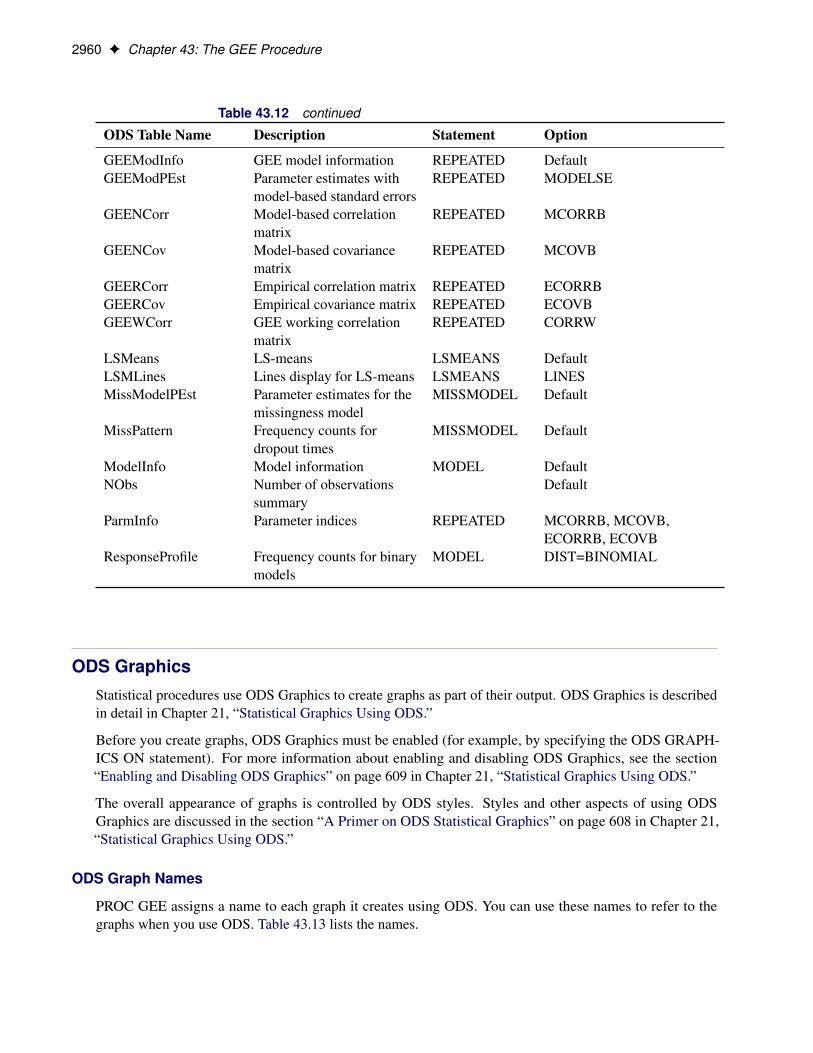
2960 F Chapter 43: The GEE Procedure
Table 43.12 continued
ODS Table Name Description Statement Option
GEEModInfo GEE model information REPEATED DefaultGEEModPEst Parameter estimates with
model-based standard errorsREPEATED MODELSE
GEENCorr Model-based correlationmatrix
REPEATED MCORRB
GEENCov Model-based covariancematrix
REPEATED MCOVB
GEERCorr Empirical correlation matrix REPEATED ECORRBGEERCov Empirical covariance matrix REPEATED ECOVBGEEWCorr GEE working correlation
matrixREPEATED CORRW
LSMeans LS-means LSMEANS DefaultLSMLines Lines display for LS-means LSMEANS LINESMissModelPEst Parameter estimates for the
missingness modelMISSMODEL Default
MissPattern Frequency counts fordropout times
MISSMODEL Default
ModelInfo Model information MODEL DefaultNObs Number of observations
summaryDefault
ParmInfo Parameter indices REPEATED MCORRB, MCOVB,ECORRB, ECOVB
ResponseProfile Frequency counts for binarymodels
MODEL DIST=BINOMIAL
ODS GraphicsStatistical procedures use ODS Graphics to create graphs as part of their output. ODS Graphics is describedin detail in Chapter 21, “Statistical Graphics Using ODS.”
Before you create graphs, ODS Graphics must be enabled (for example, by specifying the ODS GRAPH-ICS ON statement). For more information about enabling and disabling ODS Graphics, see the section“Enabling and Disabling ODS Graphics” on page 609 in Chapter 21, “Statistical Graphics Using ODS.”
The overall appearance of graphs is controlled by ODS styles. Styles and other aspects of using ODSGraphics are discussed in the section “A Primer on ODS Statistical Graphics” on page 608 in Chapter 21,“Statistical Graphics Using ODS.”
ODS Graph Names
PROC GEE assigns a name to each graph it creates using ODS. You can use these names to refer to thegraphs when you use ODS. Table 43.13 lists the names.

Examples: GEE Procedure F 2961
To request these graphs, ODS Graphics must be enabled and you must specify the statement and option thatare indicated in Table 43.13.
Table 43.13 Graphs Produced by PROC GEE
ODS Graph Name Description Statement Option
Histogram Histogram of predicted weightsfrom the missingness model
PROC PLOTS=
Examples: GEE ProcedureThe following examples illustrate some of the capabilities of the GEE procedure. These examples are notintended to represent definitive analyses of the data sets that are presented here.
Example 43.1: Comparison of the Marginal and Random Effect Models forBinary Data
A clinical trial (Stokes, Davis, and Koch 2012) was conducted to compare two treatments for a respiratoryillness. Patients in each of two centers were randomly assigned to two groups: one group received the activetreatment and one group received a placebo.
During treatment, respiratory status was determined for each of four visits and is represented by the variableOutcome (coded here as 0 = poor, 1 = good). The variables Center, Treatment, Sex, and Baseline (baselinerespiratory status) are classification variables that have two levels. The variable Age (age at time of entry intothe study) is a continuous variable.
All 111 patients completed the study. That is, there are no missing data for responses or covariates. Thefollowing statements create the data set Resp:
data Resp;input Center ID Treatment $ Sex $ Age Baseline Visit1-Visit4;datalines;
1 1 P M 46 0 0 0 0 01 2 P M 28 0 0 0 0 01 3 A M 23 1 1 1 1 11 4 P M 44 1 1 1 1 01 5 P F 13 1 1 1 1 11 6 A M 34 0 0 0 0 0
... more lines ...
2 51 A M 43 1 1 1 1 02 52 A F 39 0 1 1 1 12 53 A M 68 0 1 1 1 12 54 A F 63 1 1 1 1 12 55 A M 31 1 1 1 1 1;

2962 F Chapter 43: The GEE Procedure
data Resp;set Resp;Visit=1; Outcome=Visit1; output;Visit=2; Outcome=Visit2; output;Visit=3; Outcome=Visit3; output;Visit=4; Outcome=Visit4; output;
run;
Suppose yij represents the respiratory status of patient i at the jth visit, j D 1; : : : ; 4, and �ij D E.yij /represents the mean of the respiratory status. Logistic regression is commonly used to analyze binary responsedata. You can use the variance function for the binomial distribution, v.�ij / D �ij .1 � �ij /, and the logitlink function, g.�ij / D log.�ij =.1��ij //. The model for the mean is g.�ij / D xij 0ˇ, where ˇ is a vectorof regression parameters to be estimated.
The following SAS statements perform the GEE model fit:
proc gee data=Resp descend;class ID Treatment Center Sex Baseline;model Outcome=Treatment Center Sex Age Baseline /
dist=bin link=logit;repeated subject=ID(Center) / corr=exch corrw;
run;
Both the MODEL statement and the REPEATED statement are required.
In the MODEL statement, you use the DIST=BIN and LINK=LOGIT options to specify a logistic regression,and you specify Outcome as the response variable and Treatment, Center, Sex, Age, and Baseline as theexplanatory variables. The DESCEND option in the PROC GEE statement requests that the probability thatOutcome = 1 be modeled. If the DESCEND option had not been specified, the probability that Outcome = 0would be modeled by default.
You use the REPEATED statement to specify the subject and the correlation structure of the responses. TheSUBJECT=ID(CENTER) option specifies that the observations in any single cluster are uniquely identifiedby Center and ID. An equivalent specification is SUBJECT=ID*CENTER. Because the same ID valuesare used in each center, one of these specifications is needed. If ID values were unique across all centers,SUBJECT=ID could be specified. The option TYPE=EXCH specifies the exchangeable working correlationstructure.
The “Model Information” table displayed in Output 43.1.1 provides information about the specified logisticregression model and the input data set.
Output 43.1.1 Model Information
The GEE ProcedureThe GEE Procedure
Model Information
Data Set WORK.RESP
Distribution Binomial
Link Function Logit
Dependent Variable Outcome

Example 43.1: Comparison of the Marginal and Random Effect Models for Binary Data F 2963
General information about the GEE analysis is displayed in Output 43.1.2, and model fit criteria for themodel are displayed in Output 43.1.3.
Output 43.1.2 Model Fitting Information
GEE Model Information
Correlation Structure Exchangeable
Subject Effect ID(Center) (111 levels)
Number of Clusters 111
Correlation Matrix Dimension 4
Maximum Cluster Size 4
Minimum Cluster Size 4
Output 43.1.3 Model Fitting Information
GEE FitCriteria
QIC 512.5723
QICu 499.4873
The results of GEE model fitting are displayed in Output 43.1.4. If you specify no other options, the standarderrors, confidence intervals, Z scores, and p-values are based on empirical standard error estimates. You canspecify the MODELSE option in the REPEATED statement to create a table that is based on model-basedstandard error estimates.
Output 43.1.4 Results of Model Fitting
Parameter Estimates for Response Model
with Empirical Standard Error Estimates
Parameter EstimateStandard
Error
95%Confidence
Limits Z Pr > |Z|
Intercept 1.6391 0.5247 0.6107 2.6675 3.12 0.0018
Treatment A 1.2654 0.3467 0.5859 1.9448 3.65 0.0003
Treatment P 0.0000 0.0000 0.0000 0.0000 . .
Center 1 -0.6495 0.3532 -1.3418 0.0428 -1.84 0.0660
Center 2 0.0000 0.0000 0.0000 0.0000 . .
Sex F 0.1368 0.4402 -0.7261 0.9996 0.31 0.7560
Sex M 0.0000 0.0000 0.0000 0.0000 . .
Age -0.0188 0.0130 -0.0442 0.0067 -1.45 0.1480
Baseline 0 -1.8457 0.3460 -2.5238 -1.1676 -5.33 <.0001
Baseline 1 0.0000 0.0000 0.0000 0.0000 . .
Treatment and Baseline appear to be strongly influential, and Center might be marginally significant.
For comparison, a generalized linear mixed model is fitted to the data set to obtain subject-specific effects.Specifically, consider the logistic regression model,
logit.E.yij jbi // D xij 0ˇ� C bi
where the random effect bi is normally distributed with zero mean and variance, Var.bi / D �2b .

2964 F Chapter 43: The GEE Procedure
The following statements use the GLIMMIX procedure to fit a generalized linear mixed model:
proc glimmix data=Resp;class ID Treatment Center Sex Baseline;model Outcome (desc)=Treatment Center Sex Age Baseline /
dist=binary solution;random ID(Center);
run;
Output 43.1.5 displays the parameter estimates for the fixed effects in the generalized linear mixed model.
Output 43.1.5 Parameter Estimates
The GLIMMIX ProcedureThe GLIMMIX Procedure
Solutions for Fixed Effects
Effect Treatment Sex Center Baseline EstimateStandard
Error DF t Value Pr > |t|
Intercept 1.7936 0.6292 105 2.85 0.0053
Treatment A 1.4758 0.3898 333 3.79 0.0002
Treatment P 0 . . . .
Center 1 -0.7201 0.4051 105 -1.78 0.0784
Center 2 0 . . . .
Sex F 0.1732 0.5034 333 0.34 0.7310
Sex M 0 . . . .
Age -0.02011 0.01507 333 -1.33 0.1831
Baseline 0 -2.1343 0.3971 333 -5.38 <.0001
Baseline 1 0 . . . .
From Output 43.1.4 and Output 43.1.5, you can see that the parameter estimates from the marginal modeland the mixed-effects model differ. For example, the estimated treatment effects are 1.2654 and 1.4758 fromthe marginal model and the mixed-effects model, respectively.
The interpretation of the model effects in the marginal and random models differs. For example, the estimatedtreatment effect from the marginal model indicates that, on average, the odds of a good response for thepatients is e1:2654 D 3:5 times higher when they receive the active treatment versus the placebo. Theestimated treatment effect from the generalized linear mixed model indicates that an individual patient’s oddsof a good response is e1:4758 D 4:4 times higher when the patient receives the active treatment versus theplacebo.
The choice of the marginal model or a subject-specific model often depends on the goal of your analysis:whether you are interested in population-averaged effects or subject-specific effects. For more information,see Diggle et al. (2002); Fitzmaurice, Laird, and Ware (2011).
Example 43.2: Log-Linear Model for Count DataThe following example demonstrates how you can fit a GEE model to count data. The data are analyzed byDiggle, Liang, and Zeger (1994). The response is the number of epileptic seizures, which was measuredat the end of each of eight two-week treatment periods over sixteen weeks. The first eight weeks were thebaseline period (during which no treatment was given), and the second eight weeks were the treatment period,
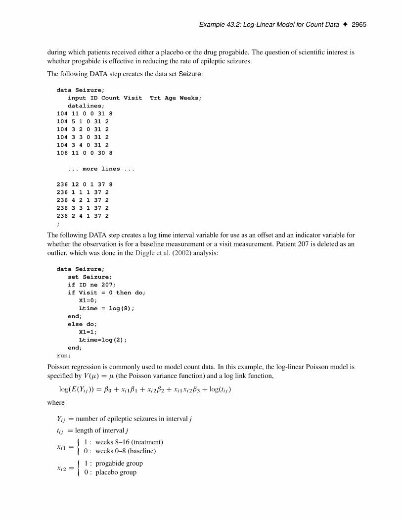
Example 43.2: Log-Linear Model for Count Data F 2965
during which patients received either a placebo or the drug progabide. The question of scientific interest iswhether progabide is effective in reducing the rate of epileptic seizures.
The following DATA step creates the data set Seizure:
data Seizure;input ID Count Visit Trt Age Weeks;datalines;
104 11 0 0 31 8104 5 1 0 31 2104 3 2 0 31 2104 3 3 0 31 2104 3 4 0 31 2106 11 0 0 30 8
... more lines ...
236 12 0 1 37 8236 1 1 1 37 2236 4 2 1 37 2236 3 3 1 37 2236 2 4 1 37 2;
The following DATA step creates a log time interval variable for use as an offset and an indicator variable forwhether the observation is for a baseline measurement or a visit measurement. Patient 207 is deleted as anoutlier, which was done in the Diggle et al. (2002) analysis:
data Seizure;set Seizure;if ID ne 207;if Visit = 0 then do;
X1=0;Ltime = log(8);
end;else do;
X1=1;Ltime=log(2);
end;run;
Poisson regression is commonly used to model count data. In this example, the log-linear Poisson model isspecified by V.�/ D � (the Poisson variance function) and a log link function,
log.E.Yij // D ˇ0 C xi1ˇ1 C xi2ˇ2 C xi1xi2ˇ3 C log.tij /
where
Yij D number of epileptic seizures in interval j
tij D length of interval j
xi1 D
�1 W weeks 8–16 (treatment)0 W weeks 0–8 (baseline)
xi2 D
�1 W progabide group0 W placebo group

2966 F Chapter 43: The GEE Procedure
Because the visits represent repeated measurements, the responses from the same individual are correlatedand inferences need to take this into account. The correlations between the counts are modeled as rij D ˛,i ¤ j (exchangeable correlations).
In this model, the regression parameters are interpreted in terms of the log seizure rate that is displayed inTable 43.14.
Table 43.14 Interpretation of Regression Parameters
Treatment Visit log.E.Yij /=tij /
Placebo Baseline ˇ01–4 ˇ0 C ˇ1
Progabide Baseline ˇ0 C ˇ21–4 ˇ0 C ˇ1 C ˇ2 C ˇ3
The difference between the log seizure rates in the pretreatment (baseline) period and the treatment periods isˇ1 for the placebo group and ˇ1 C ˇ3 for the progabide group. A value of ˇ3 < 0 indicates a reduction inthe seizure rate.
The following statements perform the analysis:
proc gee data = Seizure;class ID Visit;model Count = X1 Trt X1*Trt / dist=poisson link=log offset= Ltime;repeated subject = ID / within = Visit type=unstr covb corrw;
run;
In the MODEL statement, Count is the response variable, and X1, Trt, and the interaction X1*Trt are theexplanatory variables. You request Poisson regression with the DIST=POISSON and the LINK=LOG options.The offset variable is often used in Poisson regression to account for different exposures. In this case, theOFFSET= option specifies Ltime as the offset variable representing different time intervals.
In the REPEATED statement, the SUBJECT= option indicates that the variable ID identifies the observationsfrom a single cluster, and the TYPE=UNSTR option specifies the unstructured working correlation structure.The CORRW option requests that the working correlation matrix be displayed.
The “Model Information” table that is displayed in Output 43.2.1 provides information about the specifiedmodel and the input data set.
Output 43.2.1 Model Information
The GEE ProcedureThe GEE Procedure
Model Information
Data Set WORK.SEIZURE
Distribution Poisson
Link Function Log
Dependent Variable Count
Offset Variable Ltime
Output 43.2.2 displays general information about the GEE model analysis.

Example 43.2: Log-Linear Model for Count Data F 2967
Output 43.2.2 GEE Model Information
GEE Model Information
Correlation Structure Unstructured
Within-Subject Effect Visit (5 levels)
Subject Effect ID (58 levels)
Number of Clusters 58
Correlation Matrix Dimension 5
Maximum Cluster Size 5
Minimum Cluster Size 5
Output 43.2.3 displays the parameter estimate covariance matrices, which are requested by the COVB option.Both model-based and empirical covariances are produced.
Output 43.2.3 Covariance Matrices of Parameter Estimate
Covariance Matrix (Model-Based)
Prm1 Prm2 Prm3 Prm4
Prm1 0.01210 0.004902 -0.01210 -0.004902
Prm2 0.004902 0.006660 -0.004902 -0.006660
Prm3 -0.01210 -0.004902 0.02461 0.01299
Prm4 -0.004902 -0.006660 0.01299 0.01852
Covariance Matrix (Empirical)
Prm1 Prm2 Prm3 Prm4
Prm1 0.02597 -0.003069 -0.02597 0.003069
Prm2 -0.003069 0.008597 0.003069 -0.008597
Prm3 -0.02597 0.003069 0.03841 -0.006196
Prm4 0.003069 -0.008597 -0.006196 0.02237
The exchangeable working correlation matrix is displayed in Output 43.2.4. It shows that there are noticeablecorrelations among the respective visits.
Output 43.2.4 Working Correlation Matrix
Working Correlation Matrix
Obs 1 Obs 2 Obs 3 Obs 4 Obs 5
Obs 1 1.0000 0.7920 0.7190 0.8111 0.6582
Obs 2 0.7920 1.0000 0.4859 0.6552 0.4566
Obs 3 0.7190 0.4859 1.0000 0.6988 0.4171
Obs 4 0.8111 0.6552 0.6988 1.0000 0.6464
Obs 5 0.6582 0.4566 0.4171 0.6464 1.0000
The parameter estimates table, shown in Output 43.2.5, contains parameter estimates, standard errors,confidence intervals, Z scores, and p-values for the parameter estimates. Empirical standard error estimatesare used in this table.
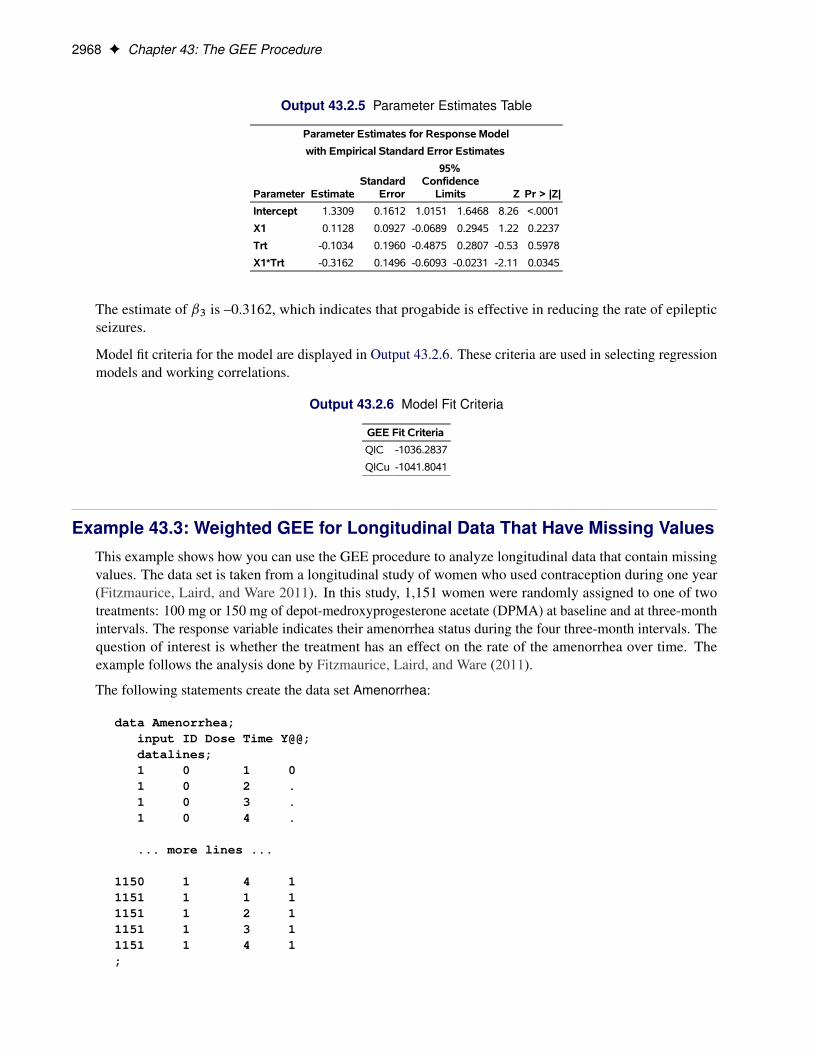
2968 F Chapter 43: The GEE Procedure
Output 43.2.5 Parameter Estimates Table
Parameter Estimates for Response Model
with Empirical Standard Error Estimates
Parameter EstimateStandard
Error
95%Confidence
Limits Z Pr > |Z|
Intercept 1.3309 0.1612 1.0151 1.6468 8.26 <.0001
X1 0.1128 0.0927 -0.0689 0.2945 1.22 0.2237
Trt -0.1034 0.1960 -0.4875 0.2807 -0.53 0.5978
X1*Trt -0.3162 0.1496 -0.6093 -0.0231 -2.11 0.0345
The estimate of ˇ3 is –0.3162, which indicates that progabide is effective in reducing the rate of epilepticseizures.
Model fit criteria for the model are displayed in Output 43.2.6. These criteria are used in selecting regressionmodels and working correlations.
Output 43.2.6 Model Fit Criteria
GEE Fit Criteria
QIC -1036.2837
QICu -1041.8041
Example 43.3: Weighted GEE for Longitudinal Data That Have Missing ValuesThis example shows how you can use the GEE procedure to analyze longitudinal data that contain missingvalues. The data set is taken from a longitudinal study of women who used contraception during one year(Fitzmaurice, Laird, and Ware 2011). In this study, 1,151 women were randomly assigned to one of twotreatments: 100 mg or 150 mg of depot-medroxyprogesterone acetate (DPMA) at baseline and at three-monthintervals. The response variable indicates their amenorrhea status during the four three-month intervals. Thequestion of interest is whether the treatment has an effect on the rate of the amenorrhea over time. Theexample follows the analysis done by Fitzmaurice, Laird, and Ware (2011).
The following statements create the data set Amenorrhea:
data Amenorrhea;input ID Dose Time Y@@;datalines;1 0 1 01 0 2 .1 0 3 .1 0 4 .
... more lines ...
1150 1 4 11151 1 1 11151 1 2 11151 1 3 11151 1 4 1;

Example 43.3: Weighted GEE for Longitudinal Data That Have Missing Values F 2969
The variables in the data are as follows:
� ID: patient’s ID
� Y: indicator of amenorrhea status (1 for amenorrhea; 0 otherwise)
� Time: four consecutive three-month intervals with values 1, 2, 3, and 4
� Dose: 0 for treatment with 100 mg injection; 1 for treatment with 150 mg injection
To prepare for the analysis, two additional variables are created:
� Prevy: the patient’s amenorrhea status in the previous three-month interval. For the baseline visit, thisis set to an arbitrary nonmissing value (0 here). In this release of PROC GEE, this arbitrary valuemust be nonmissing and valid for the response variable—for example, it should be 0 or 1 for a binaryresponse—but it does not otherwise affect the results.
� Ctime: a copy of Time, which you can include in the marginal model as a continuous effect and also inthe missingness model as a classification effect
The following statements add these two variables to the data set:
data Amenorrhea;set Amenorrhea;by ID;Prevy=lag(Y);if first.id then Prevy=0;Time=Time-1;Ctime=Time;
run;
Suppose yij denotes the amenorrhea status of woman i at the jth visit, j D 1; : : : ; 4, and suppose �ij DP.yij D 1/ denotes the average rate of high dosage. To explore whether the treatment has an effect on therate of amenorrhea over time, consider the following marginal model:
logit.�ij / D ˇ0 C ˇ1timeij C ˇ2time2ij C ˇ3dosei C ˇ4dosei � timeC ˇ5dosei � time2
Of the 1,151 women in this study, 576 are from the low-dose group, and 575 are from the high-dose group.For the low-dose group, 62.67% of the women completed the trial; for the high-dose group, 61.39% of thewomen completed this trial. Thus, both groups have substantial dropouts.
To obtain the weights for the weighted GEE analysis, consider the following logistic regression model formissingness:
logitp.rij D 1jrij�1 D 1; dosei ; ctimeij ; yij�1/ D˛0 C ˛1I.ctimeij D 1/C ˛2I.ctimeij D 2/C ˛3dosei C ˛4yij�1 C ˛5dosei � yij�1
The following statements use the observation-specific weighted GEE method and the specified response andmissingness models to analyze the data:

2970 F Chapter 43: The GEE Procedure
ods graphics on;proc gee data=Amenorrhea desc plots=histogram;
class ID Ctime;missmodel Ctime Prevy Dose Dose*Prevy / type=obslevel;model Y = Time Dose Time*Time Dose*Time Dose*Time*Time / dist=bin;repeated subject=ID / within=Ctime corr=cs;
run;
The MODEL statement specifies logistic regression and the model effects. The DESCEND option in thePROC GEE statement models the probability that Y = 1.
The REPEATED statement requests GEE analysis. The SUBJECT=ID option specifies that observationsfrom the same subject are identified by ID. The TYPE=CS option specifies the compound symmetric workingcorrelation structure.
The MISSMODEL statement requests the weighted GEE analysis. It specifies the logistic regression modelfor missingness. Note that no response variable is needed in weighted GEE analysis to specify a missingnessmodel because the response is completely determined by the response variable in the MODEL statement.Without the MISSMODEL statement, PROC GEE would use the standard GEE approach, the same asprovided by PROC GENMOD. The TYPE=OBSLEVEL option requests observation-specific weights.
Output 43.3.1 shows the parameter estimates for the missingness model. The estimate of ˛4 is –0.4514 with ap-value of 0.0053, which suggests that the possibility that a participant will drop out is related to her previousamenorrhea status. This suggests that the assumption of MAR is more appropriate than that of MCAR.
Output 43.3.1 Parameter Estimates for the Missingness Model
Parameter Estimates for Missingness Model
Parameter EstimateStandard
Error
95%Confidence
Limits Z Pr > |Z|
Intercept 2.3967 0.1438 2.1149 2.6785 16.67 <.0001
Ctime 0 0.0000 0.0000 0.0000 0.0000 . .
Ctime 1 -0.7286 0.1439 -1.0106 -0.4466 -5.06 <.0001
Ctime 2 -0.5919 0.1469 -0.8798 -0.3040 -4.03 <.0001
Ctime 3 0.0000 0.0000 0.0000 0.0000 . .
Prevy -0.4514 0.1619 -0.7687 -0.1341 -2.79 0.0053
Dose 0.0680 0.1313 -0.1893 0.3253 0.52 0.6046
Prevy*Dose -0.2381 0.2196 -0.6685 0.1923 -1.08 0.2782
The classification variable Ctime has two levels whose estimates are equal to zero. One is the reference levelCtime = 3. The first level, Ctime = 0, also has an estimate of zero, because the first visit is always observedand the first level is never used in estimating the weights in the missing model.
Output 43.3.2 displays the results of the weighted GEE analysis.

Example 43.3: Weighted GEE for Longitudinal Data That Have Missing Values F 2971
Output 43.3.2 Parameter Estimates for Amenorrhea Data Analysis Using Weighted GEE
The GEE ProcedureThe GEE Procedure
Parameter Estimates for Response Model
with Empirical Standard Error Estimates
Parameter EstimateStandard
Error
95%Confidence
Limits Z Pr > |Z|
Intercept -1.4965 0.1072 -1.7067 -1.2863 -13.95 <.0001
Time 0.5379 0.1334 0.2764 0.7994 4.03 <.0001
Dose 0.1061 0.1491 -0.1861 0.3983 0.71 0.4767
Time*Time -0.0037 0.0405 -0.0831 0.0757 -0.09 0.9275
Dose*Time 0.4092 0.1903 0.0362 0.7823 2.15 0.0315
Dose*Time*Time -0.1264 0.0577 -0.2395 -0.0134 -2.19 0.0284
The estimate of ˇ4 (the parameter estimate for the Dose*Time interaction) is 0.4092, which indicates that thechange of amenorrhea rate over time depends on the dose of DMPA. Specifically, for women in the low-dosegroup, the amenorrhea rates �ij at the four consecutive time intervals are 0.1830, 0.2764, 0.3928, and 0.5210and for women in the high-dose group, the amenorrhea rate are 0.1997, 0.3609, 0.4963, and 0.5701. In otherwords, the amenorrhea rate increases over time for both treatments, and the rates of increase are slightlydifferent.
You can request subject-level weights by specifying the TYPE=SUBLEVEL option. The results (notshown here) from the subject-level weighted method are similar to the results from the observation-levelweighted method. Both of the weighted GEE methods provide unbiased regression parameter estimates if themissingness model is specified correctly. Preisser, Lohman, and Rathouz (2002) note that the observation-level weighted GEE produces more efficient estimates than the cluster-level weighted GEE produces forincomplete longitudinal binary data.
Large weights can have impacts on the parameter estimates. Consequently, it is recommended that you checkthe distribution of the estimated weights. If there are large weights, you might consider trimming themby specifying the MAXWEIGHT= option in the MISSMODEL statement. Output 43.3.3 shows that theestimated weights in this example range between 1 and 2.1, so no trimming is needed.

2972 F Chapter 43: The GEE Procedure
Output 43.3.3 Histogram of Estimated Weights
Example 43.4: GEE for Binary Data with Logit Link FunctionBecause the respiratory data in Example 43.1 are binary, you can use the alternating logistic regression (ALR)method and model associations by using the log odds ratios instead of working correlations. This examplefits a “fully parameterized cluster” model for the log odds ratio. That is, there is a log odds ratio parameterfor each unique pair of responses within clusters, and all clusters are parameterized identically. The followingstatements fit the same regression model for the mean as in Example 43.1 but use a regression model for thelog odds ratios instead of a working correlation. LOGOR=FULLCLUST specifies a fully parameterized logodds ratio model.
proc gee data=Resp descend;class ID Treatment Center Sex Baseline;model Outcome=Treatment Center Sex Age Baseline / dist=bin;repeated subject=ID(Center) / logor=fullclust;
run;
The results of fitting the model are displayed in Output 43.4.1.

Example 43.4: GEE for Binary Data with Logit Link Function F 2973
Output 43.4.1 Results of ALR Model Fitting
The GEE ProcedureThe GEE Procedure
Parameter Estimates for Response Model
with Empirical Standard Error Estimates
Parameter EstimateStandard
Error
95%Confidence
Limits Z Pr > |Z|
Intercept 1.6001 0.5128 0.5950 2.6052 3.12 0.0018
Treatment A 1.2611 0.3406 0.5934 1.9287 3.70 0.0002
Treatment P 0.0000 0.0000 0.0000 0.0000 . .
Center 1 -0.6287 0.3486 -1.3119 0.0545 -1.80 0.0713
Center 2 0.0000 0.0000 0.0000 0.0000 . .
Sex F 0.1024 0.4362 -0.7526 0.9575 0.23 0.8144
Sex M 0.0000 0.0000 0.0000 0.0000 . .
Age -0.0162 0.0125 -0.0407 0.0084 -1.29 0.1977
Baseline 0 -1.8980 0.3404 -2.5652 -1.2308 -5.58 <.0001
Baseline 1 0.0000 0.0000 0.0000 0.0000 . .
Alpha1 1.6109 0.4892 0.6522 2.5696 3.29 0.0010
Alpha2 1.0771 0.4834 0.1297 2.0246 2.23 0.0259
Alpha3 1.5875 0.4735 0.6594 2.5155 3.35 0.0008
Alpha4 2.1224 0.5022 1.1381 3.1068 4.23 <.0001
Alpha5 1.8818 0.4686 0.9634 2.8001 4.02 <.0001
Alpha6 2.1046 0.4949 1.1347 3.0745 4.25 <.0001
The parameters Alpha1 through Alpha6 estimate the log odds ratio for each unique within-cluster pair. Thecorrespondence between the log odds ratio parameters and within-cluster pairs is displayed in Output 43.4.2.
Output 43.4.2 Log Odds Ratio Parameters
Log Odds RatioParameterInformation
Parameter Group
Alpha1 (1, 2)
Alpha2 (1, 3)
Alpha3 (1, 4)
Alpha4 (2, 3)
Alpha5 (2, 4)
Alpha6 (3, 4)
Model goodness-of-fit criteria are shown in Output 43.4.3.
Output 43.4.3 ALR Model Fit Criteria
GEE FitCriteria
QIC 511.8589
QICu 499.6516

2974 F Chapter 43: The GEE Procedure
The QIC for the ALR model shown in Output 43.4.3 is 511.86, whereas the QIC for the unstructured workingcorrelation model shown in Output 43.1.3 is 512.34, indicating that the ALR model has a slightly better fit.
You can fit the same model by fully specifying the z matrix; for the definition of the z matrix, see the section“Specifying Log Odds Ratio Models” on page 2953. The following statements create a data set that containsthe full z matrix:
data zin;keep id center z1-z6 y1 y2;array zin(6) z1-z6;set resp;by center id;if first.id
then do;t = 0;do m = 1 to 4;
do n = m+1 to 4;do j = 1 to 6;
zin(j) = 0;end;y1 = m;y2 = n;t + 1;zin(t) = 1;output;
end;end;
end;run;
proc print data=zin (obs=12);run;
Output 43.4.4 displays the full z matrix for the first two clusters. The z matrix is identical for all clusters inthis example.
Output 43.4.4 Full z Matrix Data Set
Obs z1 z2 z3 z4 z5 z6 Center ID y1 y2
1 1 0 0 0 0 0 1 1 1 2
2 0 1 0 0 0 0 1 1 1 3
3 0 0 1 0 0 0 1 1 1 4
4 0 0 0 1 0 0 1 1 2 3
5 0 0 0 0 1 0 1 1 2 4
6 0 0 0 0 0 1 1 1 3 4
7 1 0 0 0 0 0 1 2 1 2
8 0 1 0 0 0 0 1 2 1 3
9 0 0 1 0 0 0 1 2 1 4
10 0 0 0 1 0 0 1 2 2 3
11 0 0 0 0 1 0 1 2 2 4
12 0 0 0 0 0 1 1 2 3 4

Example 43.5: Alternating Logistic Regression for Ordinal Multinomial Data F 2975
The following statements fit the model for fully parameterized clusters by fully specifying the z matrix. Theresults are identical to those shown previously.
proc gee data=Resp descend;class ID Treatment Center Sex Baseline;model Outcome=Treatment Center Sex Age Baseline / dist=bin;repeated subject=ID(Center) / logor=zfull
zdata=zinzrow =(z1-z6)ypair=(y1 y2);
run;
Example 43.5: Alternating Logistic Regression for Ordinal Multinomial DataThis example illustrates how you use the GEE procedure and alternating logistic regression (ALR) to analyzeordinal multinomial data. A clinical trial was conducted to evaluate the effectiveness of the drug auranofinfor treating arthritis (Lipsitz, Kim, and Zhao 1994). Patients were assigned to one of two groups: one groupwas treated with auranofin, and the other group received a placebo. The treatment that a patient received isrecorded in the variable Treatment (coded here as 1 = auranofin and 0 = placebo).
The response was self-assessment of arthritis recorded at one-, three-, and five-month follow-up visits. Theresponses are recorded in the Rating variable and are coded as 1 = very poor, 2 = poor, 3 = fair, 4 = good, and5 = very good. This coding of Rating is finer than the coding in Lipsitz, Kim, and Zhao (1994), where onlythree levels were used. The visit numbers are recorded in the classification variable Visit, whose value is 1,3, or 5. An initial self-assessment that uses the same coding as Rating is recorded in the variable Baseline.The variable Age records the participants’ ages (in years) at the baseline visit and is treated as a continuousvariable. One participant missed all visits and is not considered. There are an additional 15 missed visits fromeight participants who dropped out, and there are four participants who missed a single visit. A weightedGEE is not used because the GEE procedure in SAS/STAT 14.1 does not support the weighted GEE methodfor the multinomial distribution.
The following DATA step creates the data set Arthritis:
data Arthritis;input ID Rating Sex Age Treatment Baseline Visit;datalines;
1 4 2 54 2 2 11 5 2 54 2 2 31 5 2 54 2 2 52 4 1 41 1 3 12 4 1 41 1 3 32 4 1 41 1 3 5
... more lines ...
301 2 2 64 1 2 5302 2 2 55 1 2 1302 3 2 55 1 2 3302 3 2 55 1 2 5;

2976 F Chapter 43: The GEE Procedure
The following SAS statements use PROC GEE to fit a model that has a fully exchangeable working correlationstructure:
proc gee data=Arthritis;class Sex ID Treatment Baseline Visit;model Rating= Visit Treatment Baseline / dist=multinomial;repeated subject=ID / within=Visit logor=exch;
run;
You specify LOGOR=EXCH in the REPEATED statement to select the ALR method that has a fullyexchangeable model for the log odds ratio. The results of the ALR model fitting are displayed in Output 43.5.1.
Output 43.5.1 Parameter Estimates for Arthritis Data Using ALR
The GEE ProcedureThe GEE Procedure
Parameter Estimates for Response Model
with Empirical Standard Error Estimates
Parameter EstimateStandard
Error
95%Confidence
Limits Z Pr > |Z|
Intercept1 -6.7502 0.4267 -7.5865 -5.9138 -15.82 <.0001
Intercept2 -4.6310 0.3968 -5.4087 -3.8533 -11.67 <.0001
Intercept3 -2.6735 0.3749 -3.4083 -1.9387 -7.13 <.0001
Intercept4 -0.3838 0.3710 -1.1109 0.3433 -1.03 0.3008
Visit 1 0.3740 0.1148 0.1489 0.5991 3.26 0.0011
Visit 3 0.3641 0.1116 0.1455 0.5828 3.26 0.0011
Visit 5 0.0000 0.0000 0.0000 0.0000 . .
Treatment 1 0.5552 0.1673 0.2273 0.8830 3.32 0.0009
Treatment 2 0.0000 0.0000 0.0000 0.0000 . .
Baseline 1 3.9457 0.5352 2.8969 4.9946 7.37 <.0001
Baseline 2 3.3052 0.4268 2.4686 4.1418 7.74 <.0001
Baseline 3 2.7483 0.3790 2.0054 3.4911 7.25 <.0001
Baseline 4 1.4013 0.4132 0.5914 2.2113 3.39 0.0007
Baseline 5 0.0000 0.0000 0.0000 0.0000 . .
Alpha1 1.6447 0.1693 1.3130 1.9764 9.72 <.0001
The parameter Alpha1, which is used to estimate the log odds ratio, is included in Output 43.5.1.
To fit the ALR model, each response is coded as a vector of binary variables and the log odds ratio models theassociation between pairs of responses. For more information about the log odds ratio and the ALR methodfor ordinal multinomial data, see the section “ALR for Ordinal Multinomial Data” on page 2952. The ALRmodel fit criteria are shown in Output 43.5.2.
Output 43.5.2 ALR Model Fit Criteria
GEE Fit Criteria
QIC 2241.9540
QICu 2259.8575

Example 43.5: Alternating Logistic Regression for Ordinal Multinomial Data F 2977
For comparison, the following SAS statements use PROC GEE to fit the same marginal model by using anindependent working correlation structure:
proc gee data=Arthritis;class Sex ID Treatment Baseline Visit;model Rating= Visit Treatment Baseline / dist=multinomial;repeated subject=ID / within=Visit;
run;
When the data have multinomial responses, the independent working correlation structure is the only structuresupported for ordinary GEEs. In Output 43.5.1 and Output 43.5.3, you can see slight differences in theparameter estimates between the model that you fit by using ALR and the model that you fit by using anindependent working correlation structure.
Output 43.5.3 Parameter Estimates for Arthritis Data Using Independent Working Correlation
The GEE ProcedureThe GEE Procedure
Parameter Estimates for Response Model
with Empirical Standard Error Estimates
Parameter EstimateStandard
Error
95%Confidence
Limits Z Pr > |Z|
Intercept1 -6.7528 0.4227 -7.5812 -5.9244 -15.98 <.0001
Intercept2 -4.6719 0.3953 -5.4466 -3.8972 -11.82 <.0001
Intercept3 -2.7138 0.3730 -3.4449 -1.9828 -7.28 <.0001
Intercept4 -0.4129 0.3689 -1.1360 0.3102 -1.12 0.2631
Visit 1 0.3852 0.1160 0.1578 0.6125 3.32 0.0009
Visit 3 0.3725 0.1118 0.1534 0.5916 3.33 0.0009
Visit 5 0.0000 0.0000 0.0000 0.0000 . .
Treatment 1 0.5643 0.1679 0.2352 0.8933 3.36 0.0008
Treatment 2 0.0000 0.0000 0.0000 0.0000 . .
Baseline 1 3.9533 0.5351 2.9046 5.0020 7.39 <.0001
Baseline 2 3.3264 0.4250 2.4934 4.1593 7.83 <.0001
Baseline 3 2.7672 0.3769 2.0285 3.5059 7.34 <.0001
Baseline 4 1.4252 0.4112 0.6192 2.2312 3.47 0.0005
Baseline 5 0.0000 0.0000 0.0000 0.0000 . .
The QIC for the ALR model shown in Output 43.5.2 is 2241.95, whereas the QIC for the independentworking correlation model shown in Output 43.5.4 is 2269.82, indicating a slightly better fit for the ALRmodel.
Output 43.5.4 Model Fit Criteria
GEE Fit Criteria
QIC 2269.8166
QICu 2259.7693

2978 F Chapter 43: The GEE Procedure
Example 43.6: GEE for Nominal Multinomial DataThis example illustrates how you use the GEE procedure to analyze nominal multinomial data. A two-yearstudy was conducted to assess the impact of access to Section 8 housing as a means of providing independenthousing to the severely mentally ill homeless (Hurlbut, Wood, and Hough 1996). In this study, half of the 362clients received Section 8 housing certificates. The assignment of Section 8 housing certificates is recordedin the variable Sec; 0 indicates clients who did not receive a certificate, and 1 indicates clients who receiveda certificate.
Every six months during the study, research staff interviewed all 362 clients, who provided data about theirliving arrangements in the previous 60 days. Clients’ living arrangements were also recorded during abaseline interview. The time of interviews is recorded in the variable Time, whose value is 0, 6, 12, or 24 (forthe number of months since the study began). There were a total of 159 missed interviews. The variableHousing records the living arrangement of a client and is coded as 0 (street living), 1 (community living), or2 (independent living). The following statements create the data set Housing:
data Housing;input ID Housing Time Sec;datalines;
1 1 0 11 2 6 11 2 12 11 2 24 12 1 0 12 2 6 1
... more lines ...
362 1 0 0362 1 6 0362 1 12 0362 1 24 0;
The following SAS statements use PROC GEE to fit a model to nominal multinomial data:
proc gee data=Housing;class ID Housing Time SEC;model Housing=Sec / dist=multinomial link=glogit;repeated subject=ID / within=Time;
run;
An ordinary GEE that has an independent working correlation structure is fit. This model is the onlyoption supported for data that have nominal multinomial responses. In the MODEL statement, you specifyLINK=GLOGIT to indicate that the responses are nominal. In the generalized logit model, you modelbaseline category logits. By default, the GEE procedure chooses the last response category as the baselinecategory. If your nominal response has J categories, then the baseline logit for category j and subject i is
log.�ij =�iJ / D �ij D x0iˇj

Example 43.6: GEE for Nominal Multinomial Data F 2979
and
�ij Dexp.�ij /PJkD1 exp.�ik/
�iJ D 0
The results of fitting the model are displayed in Output 43.6.1.
Output 43.6.1 Results of Model Fitting
The GEE ProcedureThe GEE Procedure
Parameter Estimates for Response Model
with Empirical Standard Error Estimates
Parameter Housing EstimateStandard
Error
95%Confidence
Limits Z Pr > |Z|
Intercept 0 -0.9532 0.1266 -1.2013 -0.7051 -7.53 <.0001
Intercept 1 -0.6562 0.1064 -0.8647 -0.4477 -6.17 <.0001
Sec 0 0 0.9226 0.1850 0.5599 1.2853 4.99 <.0001
Sec 0 1 1.2645 0.1642 0.9426 1.5863 7.70 <.0001
Sec 1 0 0.0000 0.0000 0.0000 0.0000 . .
Sec 1 1 0.0000 0.0000 0.0000 0.0000 . .
The positive estimates for the classification variable Sec = 0 at each response category, Housing = 0 and 1,indicate an increased probability that a client will live independently when given access to Section 8 housing.The model fit criteria are shown in Output 43.6.2
Output 43.6.2 Model Fit Criteria
GEE Fit Criteria
QIC 2675.2174
QICu 2671.4680
For comparison, the following SAS statements treat the responses as ordinal and use PROC GEE to fit amarginal model by using an independent working correlation structure:
proc gee data=Housing;class ID Housing Time SEC;model Housing=Sec / dist=multinomial;repeated subject=ID / within=Time;
run;
The cumulative logit link function is the default option that is used to fit the model. Because the generalizedlogit link function is not specified, the responses are treated as ordinal multinomial data. The results for themodel that is fit by treating the responses as ordinal are displayed in Output 43.6.3.

2980 F Chapter 43: The GEE Procedure
Output 43.6.3 Results of Model Fitting
The GEE ProcedureThe GEE Procedure
Parameter Estimates for Response Model
with Empirical Standard Error Estimates
Parameter EstimateStandard
Error
95%Confidence
Limits Z Pr > |Z|
Intercept1 -1.6917 0.1242 -1.9352 -1.4481 -13.62 <.0001
Intercept2 0.0112 0.0960 -0.1770 0.1994 0.12 0.9072
Sec 0 0.8224 0.1327 0.5624 1.0824 6.20 <.0001
Sec 1 0.0000 0.0000 0.0000 0.0000 . .
Treating the responses as ordinal results in a single parameter estimate that is related to the classificationvariable Sec. The QIC for the model that is fit by treating the responses as nominal (shown in Output 43.6.2) is2675.21, whereas the QIC for the model that is fit by treating the responses as ordinal (shown in Output 43.6.4)is 2710.50, indicating a slightly better fit when the responses are treated as nominal.
Output 43.6.4 Model Fit Criteria
GEE Fit Criteria
QIC 2710.4971
QICu 2707.2983
References
Carey, V., Zeger, S. L., and Diggle, P. J. (1993). “Modelling Multivariate Binary Data with AlternatingLogistic Regressions.” Biometrika 80:517–526.
Diggle, P. J., Heagerty, P., Liang, K.-Y., and Zeger, S. L. (2002). Analysis of Longitudinal Data. 2nd ed. NewYork: Oxford University Press.
Diggle, P. J., Liang, K.-Y., and Zeger, S. L. (1994). Analysis of Longitudinal Data. Oxford: Clarendon Press.
Fitzmaurice, G. M., Laird, N. M., and Ware, J. H. (2011). Applied Longitudinal Analysis. Hoboken, NJ: JohnWiley & Sons.
Fitzmaurice, G. M., Molenberghs, G., and Lipsitz, S. R. (1995). “Regression Models for Longitudinal BinaryResponses with Informative Drop-Outs.” Journal of the Royal Statistical Society, Series B 57:691–704.
Hardin, J. W., and Hilbe, J. M. (2003). Generalized Estimating Equations. Boca Raton, FL: Chapman &Hall/CRC.
Heagerty, P., and Zeger, S. L. (1996). “Marginal Regression Models for Clustered Ordinal Measurements.”Journal of the American Statistical Association 91:1024–1036.
Hurlbut, M. S., Wood, P. A., and Hough, R. L. (1996). “Providing Independent Housing for the HomelessMentally Ill: A Novel Approach to Evaluating Long-Term Longitudinal Housing Patterns.” Journal ofCommunity Psychology 24:291–310.

References F 2981
Liang, K.-Y., and Zeger, S. L. (1986). “Longitudinal Data Analysis Using Generalized Linear Models.”Biometrika 73:13–22.
Lipsitz, S. R., Fitzmaurice, G. M., Orav, E. J., and Laird, N. M. (1994). “Performance of GeneralizedEstimating Equations in Practical Situations.” Biometrics 50:270–278.
Lipsitz, S. R., Kim, K., and Zhao, L. (1994). “Analysis of Repeated Categorical Data Using GeneralizedEstimating Equations.” Statistics in Medicine 13:1149–1163.
Mallinckrodt, C. (2013). Preventing and Treating Missing Data in Longitudinal Clinical Trials: A PracticalGuide. Cambridge: Cambridge University Press.
McCullagh, P., and Nelder, J. A. (1989). Generalized Linear Models. 2nd ed. London: Chapman & Hall.
Molenberghs, G., and Kenward, M. G. (2007). Missing Data in Clinical Studies. New York: John Wiley &Sons.
O’Kelly, M., and Ratitch, B. (2014). Clinical Trials with Missing Data: A Guide for Practitioners. Chichester,UK: John Wiley & Sons.
Pan, W. (2001). “Akaike’s Information Criterion in Generalized Estimating Equations.” Biometrics 57:120–125.
Preisser, J. S., Lohman, K. K., and Rathouz, P. J. (2002). “Performance of Weighted Estimating Equationsfor Longitudinal Binary Data with Drop-Outs Missing at Random.” Statistics in Medicine 21:3035–3054.
Robins, J. M., and Rotnitzky, A. (1995). “Semiparametric Efficiency in Multivariate Regression Models withMissing Data.” Journal of the American Statistical Association 90:122–129.
Rubin, D. B. (1976). “Inference and Missing Data.” Biometrika 63:581–592.
Stokes, M. E., Davis, C. S., and Koch, G. G. (2012). Categorical Data Analysis Using SAS. 3rd ed. Cary,NC: SAS Institute Inc.

Subject Index
confidence intervalsconfidence coefficient, 2940
convergence criterionGEE procedure, 2945
correlated dataGEE procedure, 2948, 2955
dispersion parameter weightsGEE procedure, 2948
events/trials format for responseGEE procedure, 2940
GEE procedureconvergence criterion, 2945correlated data, 2948, 2955dispersion parameter weights, 2948events/trials format for response, 2940GEE, 2944, 2972generalized estimating equations (GEE), 2948initial values, 2945intercept, 2942logistic regression, 2930offset, 2942output ODS Graphics table names, 2960output table names, 2959QIC, 2950quasi-likelihood functions, 2951quasi-likelihood information criterion (QIC),
2950repeated measures, 2948, 2955working correlation matrix, 2945, 2946, 2949
generalized estimating equations (GEE), 2944, 2972GEE procedure, 2948
initial valuesGEE procedure, 2945
interceptGEE procedure, 2942
logistic regressionGEE procedure, 2930
offsetGEE procedure, 2942
options summaryESTIMATE statement, 2936
output ODS Graphics table namesGEE procedure, 2960
output table namesGEE procedure, 2959
probability distribution, built-inGEE procedure, 2941
QICGEE procedure, 2950
quasi-likelihood functionsGEE procedure, 2951
quasi-likelihood information criterion (QIC)GEE procedure, 2950
repeated measuresGEE procedure, 2948, 2955
weighted generalized estimating equations (WGEE),2955
working correlation matrixGEE procedure, 2945, 2946, 2949


Syntax Index
ALPHA= optionGEE procedure, MODEL statement, 2940
ALPHAINIT= optionREPEATED statement (GEE), 2945
BY statementGEE procedure, 2935
CLASS statementGEE procedure, 2935
CONVERGE= optionREPEATED statement, 2945
CORR= optionREPEATED statement , 2946
CORRB optionREPEATED statement, 2945
CORRW optionREPEATED statement, 2945
COVB optionREPEATED statement , 2945
DATA= optionPROC GEE statement, 2934
DESCENDING optionCLASS statement, 2935PROC GEE statement, 2934
DIST= optionMODEL statement, 2941
DSCALEMODEL statement, 2942
ECORRB optionREPEATED statement , 2945
ECOVB optionREPEATED statement , 2945
ERR= optionMODEL statement, 2941
ESTIMATE statementGEE procedure, 2936
FREQ statementGEE procedure, 2937
GEE proceduresyntax, 2933
GEE procedure, BY statement, 2935GEE procedure, CLASS statement, 2935
DESCENDING option, 2935ORDER= option, 2936
GEE procedure, ESTIMATE statement, 2936GEE procedure, FREQ statement, 2937GEE procedure, LSMEANS statement, 2938GEE procedure, MISSMODEL statement, 2939
MAXWEIGHT option, 2939TYPE= option, 2939
GEE procedure, MODEL statement, 2939ALPHA= option, 2940DIST= option, 2941ERR= option, 2941LINK= option, 2941NOINT option, 2942NOSCALE option, 2942OFFSET= option, 2942SCALE= option, 2942
GEE procedure, OUTPUT statement, 2942keyword= option, 2943OUT= option, 2943
GEE procedure, PROC GEE statement, 2934DATA= option, 2934DESCENDING option, 2934NAMELEN= option, 2934PLOTS option, 2934
GEE procedure, REPEATED statement, 2944ALPHAINIT= option, 2945CONVERGE= option, 2945CORR= option, 2946CORRB option, 2945CORRW option, 2945COVB option, 2945ECORRB option, 2945ECOVB option, 2945INITIAL= option, 2945INTERCEPT= option, 2945MAXITER= option, 2946MCORRB option, 2946MCOVB option, 2946MODELSE option, 2946SUBCLUSTER= option, 2946SUBJECT= option, 2944TYPE= option, 2946WITHIN= option, 2947WITHINSUBJECT= option, 2947ZDATA= option, 2947ZROW= option, 2947
GEE procedure, WEIGHT statement, 2948
INITIAL= option

REPEATED statement , 2945INTERCEPT= option
REPEATED statement , 2945
keyword= optionOUTPUT statement (GEE), 2943
LINK= optionMODEL statement, 2941
LSMEANS statementGEE procedure, 2938
MAXITER= optionREPEATED statement , 2946
MAXWEIGHT= optionMISSMODEL statement, 2939
MCORRB optionREPEATED statement , 2946
MCOVB optionREPEATED statement , 2946
MISSMODEL statementGEE procedure, 2939
MODEL statementGEE procedure, 2939
MODELSE optionREPEATED statement , 2946
NAMELEN= optionPROC GEE statement, 2934
NOINT optionMODEL statement, 2942
NOSCALE optionMODEL statement, 2942
OFFSET= optionMODEL statement, 2942
ORDER= optionCLASS statement, 2936
OUT= optionOUTPUT statement (GEE), 2943
OUTPUT statementGEE procedure, 2942
PLOTS optionPROC GEE statement, 2934
PROC GEE statement, see GEE procedurePSCALE
MODEL statement, 2942
REPEATED statementGEE procedure, 2944
SCALE= optionMODEL statement, 2942
SUBCLUSTER= option
REPEATED statement (GEE), 2946SUBJECT= option
REPEATED statement, 2944
TYPE= optionMISSMODEL statement (WGEE), 2939REPEATED statement , 2946
WEIGHT statementGEE procedure, 2948
WITHIN= optionREPEATED statement, 2947
WITHINSUBJECT= optionREPEATED statement, 2947
ZDATA= optionREPEATED statement (GEE), 2947
ZROW= optionREPEATED statement (GEE), 2947