Estimating the Gains from Liberalizing Services Trade:

The Case of Passenger Aviation*

Anca Cristea, University of Oregon

David Hummels, Purdue University & NBER

Brian Roberson, Purdue University

[September 2015, Preliminary and Incomplete]

Abstract:

Over a 22-year period the US signed 108 bilateral “Open Skies Agreements” that significantly

liberalized international trade in passenger aviation services. We study how liberalization, through

changes in route structures and the creation of international code-sharing alliances, affected consumer

welfare. We develop a novel two-stage hub-and-spoke network game in which carriers may form

alliances/code-sharing agreements and then alliances compete by setting capacity and a pricing schedule

on each of their feasible routes prior to the realization of uncertain demand. The model allows for several

empirically relevant features of airline markets: carriers may form strategic alliances; alliance route

structures feature hub-and-spoke network effects; carriers have unused capacity; prices vary across

carriers due to quality; and prices for otherwise identical seats rise as planes near capacity and are sold to

the highest valuation passengers. We further show that even complex network environments can be

described in terms of average pricing functions that provide sufficient statistics for consumer welfare, and

map closely into empirical objects. In this environment deregulation generates multiple gains for

consumers: lowering costs, increasing flight quality, and increasing carrier capacity.

We evaluate the model using difference-in-difference regressions applied to a 16-year panel of

detailed data on route structure, capacity, ticket price, quantity, and quality. Liberalizing countries see

expansions in route offerings and reallocations of carrier capacity, consistent with mechanisms

highlighted in the model. Consumers enjoy lower prices, more direct flights, and large increases in

passenger quantities conditional on prices and direct measures of quality. Consistent with the model,

these effects are not uniform across cities. Quality adjusted prices fall by 8.7 percent on routes that were

the least constrained prior to regulation, and 23 percent on the most constrained routes.

JEL: F13; L43; L93

Keywords: Services; Trade liberalization; Air transport; Open Skies Agreements.

* This paper has benefited from many helpful discussions. We particularly thank Jack Barron, Bruce Blonigen, Tim

Cason, Joe Francois, Giovanni Maggi, Steve Martin, Anson Soderbery, Bob Staiger, and Dan Trefler, and seminar

participants at Dartmouth, ITAM, Monash, Penn, Penn State, Purdue, Toronto, the World Bank, and Yale and at

several conferences including: CEPR GIST, EIIT, ETSG, Midwest International, and the West Coast Trade

Conference. We also thank John Lopresti for excellent research assistance. Any remaining errors are our own.

2

1. Introduction

Services represent a large (20 percent) and growing share of world trade, but the exact

reasons for that growth are not immediately clear. Growth in services trade may simply reflect

the rising share of services in employment and output worldwide, or be due to trade facilitating

improvements in information technology and telecommunications.1

It may also be that a

sustained focus on liberalizing services trade through the WTO General Agreement on Trade in

Services (GATS) and through bilateral agreements have succeeded in eroding regulatory barriers

to entry.2

While the literature features many papers on the effects of merchandise trade liberalization,

careful empirical work on services trade liberalization is scarce.3

The difference in research

emphasis is likely due to the paucity of detailed data on international service transactions and to

the difficulty in characterizing liberalization episodes. Feenstra et al. (2010) note that “value data

for imports and exports of services are too aggregated and their valuation questionable, while

price data are almost non-existent”. Existing regulation of services trade often takes the form of

restrictions on firm entry or complex rules governing the manner in which services are provided

and so it can be challenging to describe precisely what liberalization accomplishes. This stands

in stark contrast to manufacturing trade, where tariffs provide an exact measure of the price

wedges imposed by policy intervention, and liberalization efforts correspond to well-defined

reductions in these wedges.

This paper focuses on an internationally traded service sector, passenger aviation, where data

limitations can be overcome and where it is possible to describe and carefully model the way in

which regulations distort the provision of services. International passenger aviation is an

important service, both in size ($190 billion of trade for the US and EU in 2010) and as an input

into other international activities that require, or may be facilitated by, international movement of

persons, including: FDI, international knowledge flows, exports of complex manufactures, and

flows of other traded services.4

1 See Freund and Weinhold (2002), Ariu and Mion (2011).

2 See Hoekman et al. (2007) for a discussion on the state of services trade negotiations. Francois and Hoekman

(2010) broadly survey the literature on services trade. 3

An exception is Fink et al. (2002) who investigate the impact of telecommunication reforms on output and

productivity in a panel of developing countries. Other papers, such as Arnold et al. (2011), examine services

liberalization episodes but focus on the effects on downstream firms. 4

See Cristea (2011) and Poole (2010) for effects on exports, and Hovhannisyan and Keller (2010) for knowledge

flows.

3

Critically, and unlike many other forms of services trade, the unit of output and its price is

well defined. We draw on two datasets that contain carrier-specific data on the quantity of

passengers and ticket prices for every city pair for international flights originating or terminating

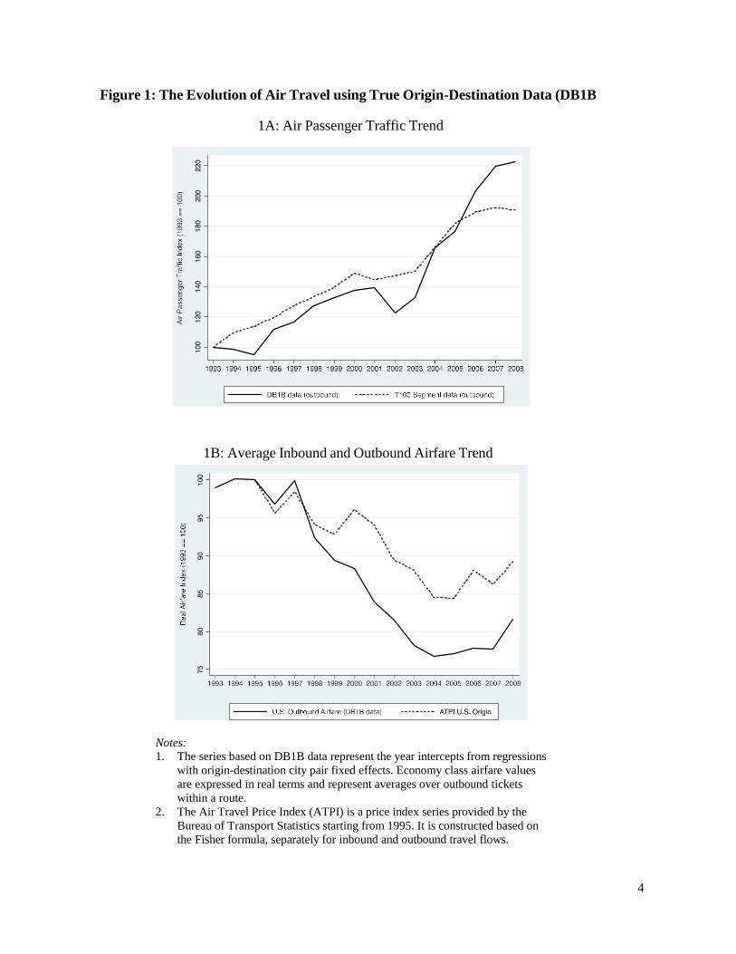
in the US from 1993-2008. Figure 1 displays passenger traffic and ticket prices in our data

between 1993 and 2008. In this period we see a doubling of US international passenger traffic,

and a 20-30 percent decline in ticket prices. What caused these changes?

One possibility is liberalization, which we discuss in greater depth in Section 2. Between

1993 and 2008, the US signed 87 bilateral “Open Skies Agreements” (OSA) that removed

barriers to trade in passenger aviation. While OSA’s altered aviation regulations in multiple

ways, we focus on several aspects that appear particularly relevant. Existing Air Service

Agreements restricted the set of “international gateway” cities into which carriers could fly,

imposed additional constraints on the number and capacity of carriers operating on these routes,

and prevented foreign competition entirely in other cities. OSAs eliminated these restrictions and

allowed for cooperative agreements including codeshares and alliances between domestic and

foreign carriers, setting the stage for potentially profound shifts in competition.

In Section 3 we model these restrictions formally using a two-stage model of international

alliance formation and capacity constrained price competition with random demand shocks. In

the first stage, alliance formation allows carriers to form alliances that decrease costs by forming

enlarged hub-and-spoke networks that pool the alliance member’s individual networks (which

are taken as given). Then, alliances choose how to route traffic through their network, set

capacity, and set prices before realizing the state of demand. We characterize the unique final-

stage local equilibrium in which carriers ration tickets to set marginal revenue equal across

demand states. The pricing function allows ticket prices to rise as carriers near the capacity

constraint of the plane with the last tickets purchased by the highest valuation consumers.

Uncertain demand yields ex-post realizations that match two key properties of this market:

otherwise identical seats sell for different prices on different days, and capacity often goes

unutilized.

We further show that the pricing functions of each carrier can be aggregated into an

analytically tractable average price function for the market. This function describes average

market prices prevailing in each period as a function of cost and demand parameters, the number

of competitors, competitors routing characteristics, and the realization of the demand shock.

4

Figure 1: The Evolution of Air Travel using True Origin-Destination Data (DB1B

1A: Air Passenger Traffic Trend

1B: Average Inbound and Outbound Airfare Trend

Notes: 1. The series based on DB1B data represent the year intercepts from regressions

with origin-destination city pair fixed effects. Economy class airfare values

are expressed in real terms and represent averages over outbound tickets

within a route.

2. The Air Travel Price Index (ATPI) is a price index series provided by the

Bureau of Transport Statistics starting from 1995. It is constructed based on

the Fisher formula, separately for inbound and outbound travel flows.

5

Complex changes in the regulatory environment can be summarized through changes in the

average price function because it is a sufficient statistic for consumer welfare (both ex-ante and

ex-post), and because it provides a tight match to the empirical objects employed in our

estimation.

To capture the key features of the changing regulatory environment, the price-capacity

competition stage is preceded by a stylized international alliance-formation stage. In the Pre-

OSA game, direct international service is only allowed between gateway cities, subject to a

policy-imposed aggregate capacity constraint. Non-gateway “hub” cities can only be reached by

indirect flights that first route through the gateway, and foreign carriers are excluded from these

cities entirely.5

Gateway restrictions impose three costs on consumers flying out of non-gateway

hubs: marginal costs are higher for indirect flights; consumers prefer direct flights and so indirect

routing is equivalent to lowering service quality; and the restriction on foreign entry lowers

competition. Consumers flying out of gateways suffer primarily from aggregate capacity

restrictions that are worsened by forcing all passengers to route through gateways.

The model highlights several changes in market structure that result from liberalization.

One, at non-gateway cities direct international connections are now possible but alliance

formation has two conflicting effects, lowering the level of competition and generating cost-

savings in the form of hub-and-spoke effects arising in each alliance’s pooled network. In

equilibrium, we find that at non-gateway cities the removal of route restrictions effect dominates

the ambiguous alliance effect and directness and quantities increase while average prices fall.

Two, at gateway cities there are no new direct international connections, and we find that in

equilibrium the alliance effect on prices and quantities is ambiguous. However, it is clear that the

relaxation of route restrictions results in a net exit of capacity flying through gateways, as

alliances opt to provide lower cost and higher quality direct service from non-gateway cities

rather than providing indirect service via gateways.

The strength of the channels highlighted in the model and the magnitudes of the associated

gains depend on the underlying parameters of the model. We turn next to empirics, describing

our data in Section 4, and our econometric exercises in Section 5.

5 Cabotage rules, in force before and after OSAs, prevent foreign carriers from offering service between any two

domestic cities. Pre-OSA, this excludes foreign carriers from reaching any non-gateway city. Post-OSA, foreign

carriers can reach any city if they are willing to offer a direct flight, plus any city in the foreign carrier’s alliance

may be reached with an indirect flight.

6

Because OSAs come into force discretely and sequentially, we can test for the effects of

liberalization using difference-in-difference strategies. That is, we measure pre/post agreement

changes in key variables (quantities, prices, capacity, route offerings) for a given country-pair or

city-pair in comparison to pairs that have not yet liberalized. This allows us to control for

changes in technology, input cost shocks, and exogenous changes in aviation demand to see

whether liberalizing countries experience differential growth in variables. We can also look at

the distribution of effects across city-pair markets to see if the core predictions of the model

(different effects for gateway and non-gateway cities) can be found in the data.

We find evidence for significant changes in market structure after liberalization. Five or

more years after the signing of an Open Skies Agreement, outbound air traffic is 17 percent

higher in liberalized markets compared to still-regulated markets. The introduction of new non-

stop routes to the liberalized foreign country explains 38 percent of this increase. Capacity rises

16 percent in liberalized markets relative to still-regulated markets, but the share of pre-OSA

gateways in that capacity falls by 13 percent. All this is consistent with the view that pre-OSA

gateway restrictions significantly reduced the desired route offerings of carriers, and both

constrained and misallocated market capacity.

We turn next to estimation focused on isolating the mechanisms through which passenger

traffic grew and in calculating consumer welfare changes associated with liberalization. Recall

that the model can be described in terms of an average pricing function and equilibrium in a

given period is given by the intersection of that average price curve with the (ex-post) demand

curve. We can then characterize OSA-related changes in the environment into changes in

average prices (moves along the demand curve), and changes in quality (shifts of the demand

curve conditional on average prices). We can also identify and estimate an explicit measure of

quality highlighted by the model, consumer’s valuation of direct routing and changes in direct

routing associated with OSAs.

We begin by estimating a series of partial derivatives, the direct effect of Open Skies

Agreements on model variables. OSAs lead to a 2-4 percent drop in average airfares (controlling

for trip characteristics). Prices are increasing in the number of segments, consistent with the

model, and decreasing in (instrumented) passengers flown, consistent with economies of route

density. The quantity of passengers flown grows 5 percent for pre-OSA gateways, 13 percent for

small cities, and 17.5 percent for large hub cities capable of accepting international traffic.

Consumers have a strong preference for direct flights, as doubling the number of flight segments

7

has an equivalent demand effect of raising prices by 50 percent. Finally, OSAs generate a 4.5

percent reduction in the number of segments a passenger flies, but only on those cities where

new direct connections occur. Passenger growth itself further reduces the number of segments

flown.

To conclude the paper we combine these partial derivatives in a system of equations to get

the total derivative of quantities and (quality-adjusted) prices with respect to OSAs. These show

profound differences across cities depending on how much liberalization relaxed constraints

facing the market. At the low end, liberalization increases quantities in pre-OSA gateways by

11.2 percent and lowers quality-adjusted prices by 8.7 percent. At the high end, liberalization

increases quantities in cities with new direct connections by 30 percent and reduces quality-

adjusted prices by 23 percent. A population-weighted average across city types shows an

aggregate decline in quality-adjusted prices of 14.4 percent.

2. Liberalization in International Air Transport Services and Related Literature.

Historically, a complex web of regulations set on a bilateral basis has restricted the provision

of international air services.6

A standard bilateral aviation agreement specifies a limited set of

gateway points/airports that can be serviced by a restricted number of designated airlines

(typically one or two carriers from each country). It also delineates the traffic rights granted to

operating carriers, the capacity that can be supplied in each origin-destination city pair (with

exact rules for sharing capacity), and the air fares to be charged on each route (with both

countries’ approval required before they can enter into effect). The prices agreed upon in the

agreements frequently correspond to the fixed rates set by IATA during periodic airfare

conferences (Doganis 2006).7

As an example, the US-China Aviation Treaty (1980) restricts market access to two

designated airlines per country, who can operate at most two round-trip flights per week each on

routes connecting four U.S. points (New York, San Francisco, Los Angeles, Honolulu) to two

Chinese cities (Shanghai, Beijing). Tokyo is the only third country location from where service

to either country's designated airports can be operated. Prices charged on all routes must be

6 Efforts to set a multilateral regulatory framework go back to the Chicago Convention of 1944 when the

International Civil Aviation Organization (ICAO) was established under the auspices of the UN. Apart from safety

and technical rules, the Convention failed to reach common grounds. Bilateral agreements became the norm and

passenger aviation remains outside the General Agreement on Trade in Services (GATS). 7

IATA (International Air Transport Association) is the trade association of international airlines and one of its main

tasks has been to fix prices on most international city-pair routes. Because IATA prices have to be agreed upon by

all member airlines, they tend to be high enough to cover the costs of the least efficient carrier (Brueckner 2003).

8

submitted to government authorities two months in advance for double approval. In addition,

both countries can take ‘appropriate’ action to ensure that traffic is ‘reasonably balanced’ and

mutually beneficial to all designated airlines.

In 1980, the United States passed the International Air Transportation Competition Act,

which set the stage for opening international aviation markets. The liberalization efforts debuted

with the renegotiation of many U.S. bilateral aviation agreements during the 1980s − the “open

markets” phase. The main focus of these treaty renewals was to relax market access and capacity

restrictions by extending the number of designated airlines, the pre-defined points of service, and

the flight frequencies. Some agreements also granted a partial relaxation of pricing provisions

and beyond traffic rights (i.e., the right to fly passengers between two pre-approved foreign

points on the way to/from a carrier's home country).

Between 1992 and 2013 the U.S. signed 108 bilateral Open Skies Agreements.8

These

agreements grant unlimited market access to any carrier for service between any two points in

the signatory countries, full flexibility in setting prices, unconstrained capacity choice and flight

frequencies, unlimited access to third country markets, and a commitment to approve inter-

airline commercial agreements (e.g., code-share, strategic alliances). The timing and complete

list of partner countries is reported in the Appendix Table A1. Apart from the completely

liberalized intra-EU aviation market, US efforts to de-regulate international aviation in this

period are atypical. While some air service agreements have been amended to relax regulatory

provisions, overall the global aviation market remains fairly closed to trade.9

We next discuss the relevant theoretical and empirical literatures to which our paper

contributes. Our model is closely related to work on hub-and-spoke networks and to models of

Bertrand-Edgeworth price competition.

In the wake of US domestic airline de-regulation, many authors explored models of hub-and-

spoke networks (e.g. Caves et al. 1984, Bailey et al 1985, Berry 1990, Brueckner and Spiller

1991, Brueckner et al. 1992, and Brueckner 2004). These models usually focus on economies of

route density and/or consumer preferences for direct flights and feature quantity competition

between firms who are free to choose network structure. Some authors, notably Hendricks et al.

(1997, 1999) argue that price-setting competition is a more appropriate environment for the

8 In this period, the US also signed a small number of partial liberalization agreements that served in several cases

as a short transitory stage before signing a full OSA. We address these partial liberalization efforts in our empirical

work. Of the 108 agreements, 87 occur within the time frame covered by our data. 9

Piermartini and Rousova (2008) provide a comprehensive description of 2300 bilateral aviation treaties in force in

2005, concluding that 70 percent of bilateral agreements worldwide are still highly restrictive.

9

airline industry, and focus on the difficulty of sustaining entry by multiple carriers when those

carriers first establish networks and then compete in prices. Models such as Aguirregabiria and

Ho (2010, 2012) feature differentiated products price-competition, which allow multiple firms to

compete in equilibrium because consumers differ in their taste for particular carriers.

Like several of these papers, our model features hub-and-spoke network effects, and allows

for carriers that are differentiated by type (direct, indirect flights) but are otherwise homogeneous

within that type. Unlike the earlier work, we sustain entry of multiple carriers of each type within

a price-setting game by assuming the existence of capacity constraints and uncertain demand.

This has two additional merits. One, the model predicts empirically relevant facts: unused

capacity and price dispersion both across firms and within a firm’s own ticket offerings. Two, we

can aggregate carrier ticket offerings into a tractable average-price function that allows us to

calculate the welfare change after liberalization without estimating consumers’ “brand loyalty”

associated with entering/exiting carriers. This feature is especially important when considering

the large number of routes we analyze, and the prevalence of multi-segment tickets offered by

alliances through a combination of its member carriers.

Our modeling approach to capacity constrained price competition is closely related to

Bertrand-Edgeworth competition (e.g. Kreps and Schienckman 1983, Osborne and Pitchik 1986,

Allen and Helliwig 1986, Deneckere and Kovenock 1996). The Bertrand-Edgeworth model is

typically formulated as a two-stage game in which firms first choose costly capacity, which is

observable, and then firms compete via prices over known demand. Each firm has a constant per

unit cost for production up to their respective capacity constraint, and each firm chooses a single

price. Demand is efficiently rationed.10

This can be thought of as a situation in which the

consumers, each with unit demand for the good and heterogeneous reservation values, form an

ordered queue that is decreasing with respect to the consumers’ reservation values. Consumers

buy from the lowest priced firm up to the point that the lowest price firm exhausts its capacity,

then move on to the second lowest price firm and so on.

Our approach, which builds upon Prescott (1975), Eden (1990), and Dana (1999) is an

incomplete information price-capacity game that features (i) intra-firm price dispersion, (ii)

demand uncertainty, and (iii) random rationing, meaning that the consumer queue is random, not

10 For an exception, see Davidson and Deneckere (1986) who use random rationing.

10

ordered. The first two distinctions, allowing each firm to sell tickets on a given route at multiple

prices and uncertain demand, are clearly critical features of our airline industry application.11

Reynolds and Wilson (2000) and Lepore (2012)12

examine demand uncertainty in the

Bertrand-Edgeworth model,13

but the information structure there differs from our framework.

Uncertain demand is modeled as a three-stage game: capacity choice, realization of the state of

the demand, and then price competition. In our framework, demand is not realized until after the

firms have chosen price-quantity schedules. Combining this information structure with intra-firm

price dispersion and random rationing, we can summarize our game as follows: (i) carriers set

capacity and choose price-quantity schedules that specify the quantity of tickets to be sold at

each price, (ii) heterogeneous consumers form a queue in which the order of reservation values is

random and the length of the queue is random, (iii) consumers buy the lowest effective (quality-

adjusted) price available tickets first, regardless of carriers, (iv) ex-post, carriers may have

unsold tickets and face a capacity cost for holding them.

We also contribute to an empirical literature on airline deregulation. Liberalization of

international aviation markets follows earlier de-regulation of US domestic markets. Studies of

the U.S. domestic airline industry have shown that the inability of airlines to compete in prices

caused them to invest in service enhancements (Borenstein and Rose 1998). Limitations in route

and capacity choices increased operating costs by restraining airlines' ability to optimize their

network structure, size and traffic density (Baltagi et. al 1995).

The liberalization of international passenger aviation services has been the focus of few

recent studies.14

Several studies employ the same datasets that we use, but very different sample

cuts, to investigate the price effects of the inter-airline strategic alliances (e.g. Brueckner and

Whalen 2000, Brueckner 2003, Whalen 2007, Bilotkach 2007). These studies find that airline

11 This is a simplification of the dynamic problem that carriers face in pricing tickets, but as shown by Escobari and

Gan (2007) this simplification appears to fit the airline industry well. For more on the airline’s dynamic pricing

problem, see the surveys in McAfee and te Velde (2006) and Aviv et al. (2012). Recent examples of this dynamic

pricing problem include Wright, et al. (2010), Deneckere and Peck (2012), Gallego and Hu (2014). 12

Issues regarding demand uncertainty and production flexibility also feature prominently in the operations

management literature. See for example Anupindi and Jiang (2008). 13

Hu (2010) and Barla and Constantatos (2005) examine demand uncertainty in the context of hub-and-spoke

network formation followed by quantity-setting competition. However, as in Reynolds and Wilson (2000) and

Lepore (2012), the state of demand is realized prior to the final stage market competition subgame. 14

Apart from passenger aviation, Micco and Serebrisky (2006) focus on air cargo, often carried in the holds of

passenger aircraft. They estimate that OSAs lowered air cargo freight rates in US imports by 9 percent.

11

alliances reduce airfares, which is consistent with our price results as OSAs facilitate the

formation of airline alliances.15

Piermartini and Rousova (2013) use a 2005 cross-section sample of worldwide country-pairs

to estimate the impact of air services liberalization on the bilateral volume of air passenger flows.

They estimate that OSAs increase traffic by 5 percent. Whalen (2007) uses similar data to ours

but a substantially different sample. He finds that OSAs increase airfares and have no effect on

passenger volumes once controlling for market competition and strategic alliances. Winston and

Yan (2013) examine the impact of liberalization on fares and passengers for a subset of heavily

trafficked international aviation routes, employing average fare data reported to IATA from

2005-2009. They employ a difference-in-difference at the country level for short run estimates,

and employ cross-country variation for identification of long run estimates. They find very large

(70 percent) reductions in average fares.

We differ from these earlier studies in three respects. One, we tie our estimates tightly to an

explicit model of the mechanisms through which OSAs liberalize markets. We demonstrate the

importance of these mechanisms in the data, and provide consumer welfare estimates that

decompose the channels of response. Two, by using a comprehensive set of ticket data that

includes connecting flights, we can demonstrate the differential impact of liberalization across

different city types, as suggested by the model. This also allows us to explore a novel mechanism

for liberalization: international connecting flights allow slow-to-sign countries to benefit from

early liberalization of their neighbor’s markets. Three, we have a longer panel which allows us to

employ difference-in-difference estimates to identify within city-pair changes in price, quantity,

and connection effects for a large number of agreements. This prevents heterogeneity across city-

pairs from affecting our results. Related, the long panel allows us to address concerns about the

endogeneity of liberalization. We restrict our samples to include only countries that sign OSAs

so that we identify effects entirely from the timing of when an agreement is signed and not by

comparing signers to non-signers.

3. Model

We study a two-stage model of international alliance formation and oligopoly price-capacity

competition in which consumers have a preference for directness. In the first stage, we consider a

stylistic model of alliance formation that takes each carrier’s domestic hub-and-spoke network as

15 These results differ from ours substantially.

12

given and then carriers from distinct countries may, via bargaining with binding commitments,

join together to form an international alliance that creates a pooled hub-and-spoke network of

international routes for the alliance. In the second stage each alliance observes the profile of first-

stage alliances, and then sets a price-quantity schedule on each of its feasible international routes,

after which uncertain demand is realized and tickets are purchased. We begin by describing the

international hub networks and then examine the first-stage alliance-formation and the final-

stage price-quantity schedule competition.

There is a domestic country 𝐴 and 𝑛! foreign countries labeled 𝐹!, 𝐹!, … , 𝐹! . Country 𝐴 is a

large country with an arbitrary number 𝑛! of carriers. Each foreign country is a small country with a single carrier. Let Ι ≡ {1, … , 𝑛! + 𝑛!} denote the set of carriers, where an arbitrary carrier (domestic or foreign) is denoted by 𝑖. There are two types of cities: (i) gateway cities that may serve as an international hub both pre- and post-OSA and (ii) non-gateway cities that are large

enough that they may serve, post-OSA, as an international hub. Each foreign country has a single city, which is a gateway city, and each foreign carrier has a hub at its gateway city. Country 𝐴 has an arbitrary number 𝑛!" of non-gateway cities, and an arbitrary number 𝑛! of gateway cities. Let 𝒥 ≡ {1, … , 𝑛!" + 𝑛! + 𝑛!} denote the set of cities, where an arbitrary city (gateway or non-gateway) is denoted by 𝑗. Each domestic carrier has hubs at a subset of its country’s cities, and we assume that each domestic carrier has at least one hub at a country 𝐴 gateway city. For each 𝑗 ∈ 𝒥, let 𝛤! denote the set of carriers with a hub at city 𝑗.

In describing feasible origin-destination paths, consider a complete graph with the node set corresponding to 𝒥, the set of all gateway and non-gateway cities. For simplicity, we restrict each origin-destination path to include at most one stop, or equivalently two links. We take the

carriers’ domestic hub-and-spoke networks as given, and model economies of scale/traffic

density arising in hub-and-spoke networks as follows.16

For travel on links connecting hubs with

non-hubs, allocating capacity to the link is costly, and we assume that this takes the form of a

constant per-unit cost of 𝜆! > 0 for an international link between country A and any foreign country (henceforth the international link) and 𝜆! ∈ (0, 𝜆!) for a connecting link within country A or between any of the foreign countries (henceforth the connecting link).

17 To account for

16 For a survey of the related hub location model see Cambell et al. (2002) or Alumur and Kara (2008). Given our

focus on international air travel, we take the carriers’ domestic networks as given and abstract from the hub location

problem that takes into account both domestic and international travel flows. 17

It is straightforward, albeit tedious, to allow for these capacity costs to be route specific and be a function of the

distance traveled on each link.

!

13

economies of scale/traffic density, travel on inter-hub links is discounted by a factor 𝛾 ∈ !!

!!!!! , 1 , which implies that 𝛾 𝜆! + 𝜆! ≥ 𝜆!

and indirect service is always at least as

expensive as direct service. Note that with one-stop origin-destination paths, direct routes may feature either 0 or 1 inter-hub links with per-unit capacity costs of 𝜆! and 𝛾𝜆! respectively. Indirect routes may feature 0, 1, or 2 inter-hub links, and the inter-hub links may either be on the international link or the connecting link. For example, an indirect route with an inter-hub

international link has a per-unit capacity cost of 𝜆! + 𝛾𝜆!, but an indirect route with an inter-hub connecting link has a per-unit capacity cost of 𝛾𝜆! + 𝜆!. Feasible origin-destination paths are constrained in that any border-crossing link in an origin-destination path offered by an alliance

(pre- and post-OSA) must takeoff from and/or land at one of the alliance’s hub cities. Pre-OSA

feasible origin-destination paths are also constrained in that any border-crossing link in an

origin-destination path must connect gateway cities.18

Post-OSA this last constraint is relaxed

and any border-crossing link of an origin-destination path may link any two cities, subject to the

restriction that border-crossing links offered by an alliance must start or end at a hub of an

alliance member.

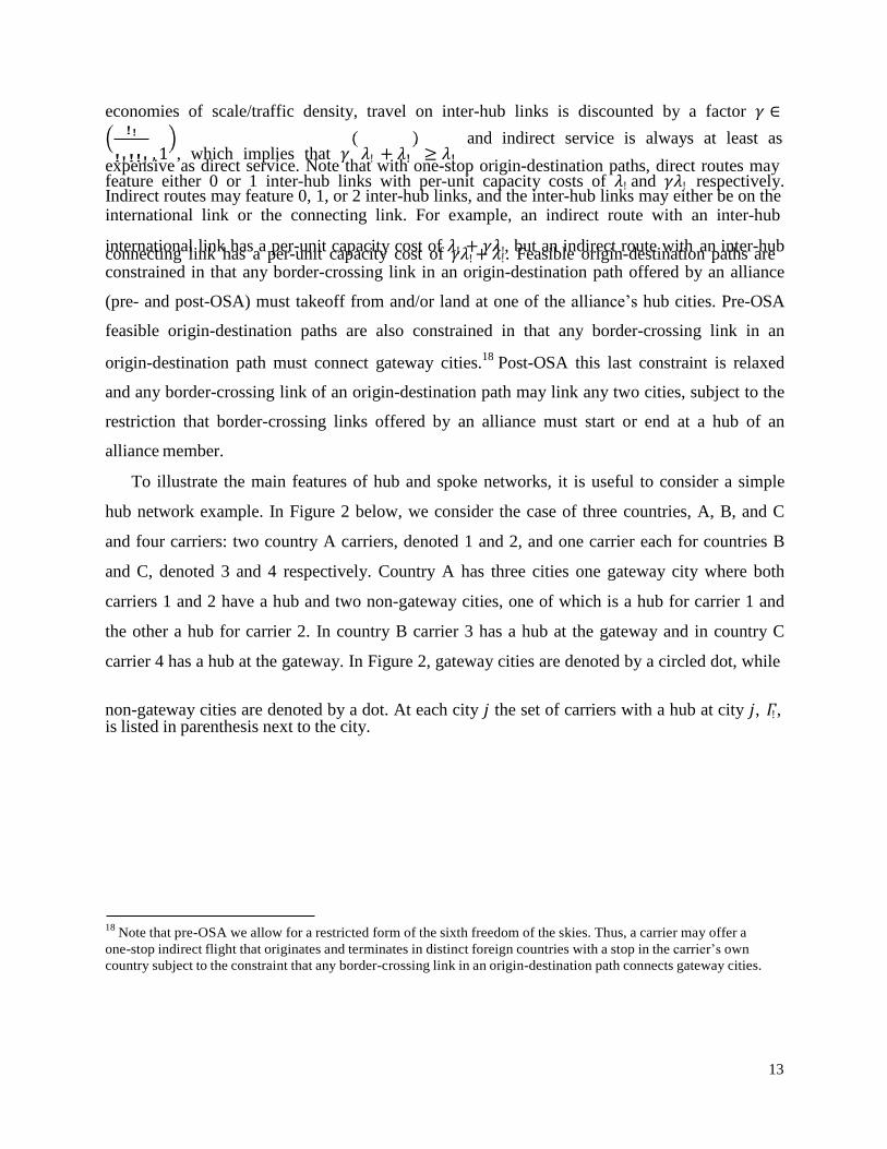
To illustrate the main features of hub and spoke networks, it is useful to consider a simple

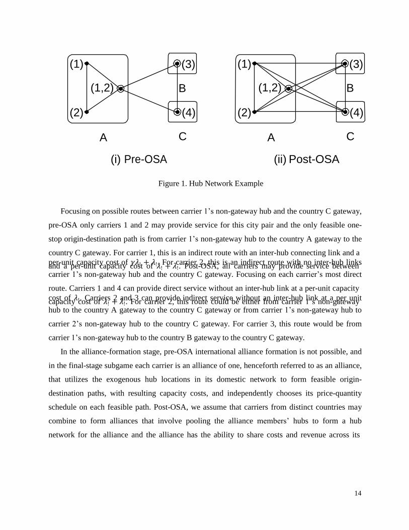
hub network example. In Figure 2 below, we consider the case of three countries, A, B, and C

and four carriers: two country A carriers, denoted 1 and 2, and one carrier each for countries B

and C, denoted 3 and 4 respectively. Country A has three cities one gateway city where both

carriers 1 and 2 have a hub and two non-gateway cities, one of which is a hub for carrier 1 and

the other a hub for carrier 2. In country B carrier 3 has a hub at the gateway and in country C

carrier 4 has a hub at the gateway. In Figure 2, gateway cities are denoted by a circled dot, while

non-gateway cities are denoted by a dot. At each city 𝑗 the set of carriers with a hub at city 𝑗, 𝛤! , is listed in parenthesis next to the city.

18 Note that pre-OSA we allow for a restricted form of the sixth freedom of the skies. Thus, a carrier may offer a

one-stop indirect flight that originates and terminates in distinct foreign countries with a stop in the carrier’s own

country subject to the constraint that any border-crossing link in an origin-destination path connects gateway cities.

14

A C A C

(i) Pre-OSA (ii) Post-OSA

Figure 1. Hub Network Example

Focusing on possible routes between carrier 1’s non-gateway hub and the country C gateway,

pre-OSA only carriers 1 and 2 may provide service for this city pair and the only feasible one-

stop origin-destination path is from carrier 1’s non-gateway hub to the country A gateway to the

country C gateway. For carrier 1, this is an indirect route with an inter-hub connecting link and a

per-unit capacity cost of 𝛾𝜆! + 𝜆!. For carrier 2, this is an indirect route with no inter-hub links and a per-unit capacity cost of 𝜆! + 𝜆!. Post-OSA, all carriers may provide service between carrier 1’s non-gateway hub and the country C gateway. Focusing on each carrier’s most direct

route. Carriers 1 and 4 can provide direct service without an inter-hub link at a per-unit capacity

cost of 𝜆!. Carriers 2 and 3 can provide indirect service without an inter-hub link at a per unit capacity cost of 𝜆! + 𝜆!. For carrier 2, this route could be either from carrier 1’s non-gateway hub to the country A gateway to the country C gateway or from carrier 1’s non-gateway hub to

carrier 2’s non-gateway hub to the country C gateway. For carrier 3, this route would be from

carrier 1’s non-gateway hub to the country B gateway to the country C gateway.

In the alliance-formation stage, pre-OSA international alliance formation is not possible, and

in the final-stage subgame each carrier is an alliance of one, henceforth referred to as an alliance,

that utilizes the exogenous hub locations in its domestic network to form feasible origin-

destination paths, with resulting capacity costs, and independently chooses its price-quantity

schedule on each feasible path. Post-OSA, we assume that carriers from distinct countries may

combine to form alliances that involve pooling the alliance members’ hubs to form a hub

network for the alliance and the alliance has the ability to share costs and revenue across its

(1,2)

(1) (3)

B

(2) (4)

(1) (3)

(1,2) B

(2) (4)

15

members. We examine a stylistic model of alliance formation that takes the payoffs from the

resulting final-stage price-quantity subgame as the primitives. Consider a partition-function game (𝑁, 𝑉) in which the payoff to each alliance (or coalition) depends not only on the identity of its member carriers but the entire partition of carriers into alliances. The set of players 𝑁 is the set of all carriers, Ι. We impose the constraint that alliances must consist of carriers from distinct countries, and let Ω denote the set of feasible partitions. The equilibrium payoffs in the final- stage subgame (for all feasible carrier partitions) generates the partition function, 𝑉(𝑆, 𝜇) which provides the total payoff to alliance 𝑆 given that 𝜇 ∈ 𝛺 is a partition of all carriers into alliances that includes alliance 𝑆 as one of the alliances.

Post-OSA our approach to alliance formation is based on the bargaining with binding

agreements approach to coalition formation in environments with externalities across coalitions

as developed in Bloch (1996), Yi (1996), and Ray and Vohra (1999).19

In particular, we assume

that alliance formation endogenously takes place in a sequential-move bargaining with binding

commitments environment along the lines of Ray and Vohra (1999). An initial proposer starts the game and chooses an alliance 𝑆, of which she is a member, and proposes a feasible division of the worth of alliance 𝑆, contingent upon each of the feasible alliance partitions given that 𝑆 has formed an alliance, among its members. The members of 𝑆 sequentially choose, in an order specified by the choice of 𝑆, to accept or reject the proposal. If all members of 𝑆 accept the proposal, then alliance 𝑆 retires from the game and the process continues for the remaining set of carriers. If a member of 𝑆 rejects the proposal, then the first rejector becomes the proposer. Rejection also imposes a cost in the form of delay, where each carrier has a common discount

factor of 𝛿 ∈ (0,1).

It is useful to examine the cost-saving effects of alliance formation in the context of the

Figure 1 example. Consider again travel between carrier 1’s non-gateway hub and the country C

gateway, and recall that post-OSA there are no route restrictions. If carriers 1 and 4 form an

alliance, then in the {1,4} alliance’s pooled hub network direct service (between carrier 1’s non-

gateway hub and the country C gateway) involves an international inter-hub link and the per-unit

cost of a direct flight is 𝛾𝜆!. Thus, the formation of the {1,4} alliance decreases each carrier’s

costs from 𝜆! to 𝛾𝜆!. The alliance also allows carriers 1 and 4 to coordinate and form a single

price-quantity schedule for the alliance on each feasible route, thereby decreasing the number of

distinct players competing on each route. Note that unlike a standard cooperative game, this

19 For more on this approach to coalition formation, see the recent survey by Ray and Vohra (2014).

16

environment features externalities across coalitions in that the payoff to each alliance depends on

the composition of each of the other alliances and the hub and spoke networks of each of the

other alliances.

In the final stage each alliance observes the profile of first-stage alliances and the resulting

hub networks for each alliance, and then sets a price-quantity schedule on each of its feasible

direct and indirect international routes, after which uncertain demand is realized and tickets are

purchased. In the final-stage price-capacity competition, we ignore directional flow issues,

impose the restriction that prices must be the same in each direction, and focus on the total

quantity of round-trip travel demanded on a given route at a given price. We also restrict our

focus to international flights that originate or terminate in country 𝐴. We now examine the final-stage price-quantity competition that provides the alliances’

payoffs for each possible alliance configuration. The final-stage demand for international air

travel has three critical elements: (i) a preference for directness, (ii) random rationing, and (iii)

demand uncertainty. In what follows we focus on travel for an arbitrary international city pair.

Beginning with the preference for directness, we assume that consumers prefer a direct flight to

an indirect flight as long as 𝛼 ∈ (0,1) times the price of the direct flight 𝑝! is less than or equal to the price of the indirect flight 𝑝!, i.e., 𝛼𝑝! ≤ 𝑝!. If 𝛼𝑝! > 𝑝!, then the indirect flight is preferred. It will be convenient to define the ‘effective’ price of a ticket 𝑝, where for an indirect

ticket with price 𝑝! the effective price is 𝑝 ≡ !

and for a direct ticket with price 𝑝! the effective !

price is 𝑝 ≡ 𝑝!.

Second, we assume random (also known as proportional) rationing. This is consistent with

heterogeneous consumers, each having unit demand and differing reservation prices, randomly

queuing and purchasing the lowest effective price tickets first, subject to availability. In addition

to the random ordering of the heterogeneous consumers in the queue, there is uncertainty

regarding the number of consumers/length of the queue, and this uncertainty is not resolved until

after carriers make their price-capacity choices.

Third, demand uncertainty for travel between an international city pair takes the form 𝑒𝐷(𝑝)

where 𝑒 is the random state of demand that is distributed according to the distribution function

𝐹(𝑒) which is twice continuously differentiable with 𝐹! 𝑒 > 0 and 𝐹!! 𝑒 ≥ 0 for 𝑒 ∈ [0,1] and

!

17

𝐹 0 = 0.20

We assume that there exists a finite price 𝑝 = inf{𝑝|𝐷 𝑝 = 0 }, and that demand is continuously differentiable with 𝐷′ 𝑝 < 0 for all 𝑝 ∈ [0, 𝑝]. We also assume that the revenue function 𝑝𝐷 𝑝 is single peaked and that the peak, denoted 𝑝!"#$ is strictly less than the choke- price 𝑝. This assumption on the revenue function implies that there exists a measurable set of prices over which total revenue is decreasing with respect to price. For the case of constant-

elasticity demand as is used in the empirical specification, the choke-price assumption implies

that CES demand be truncated at the choke price, i.e., 𝐷 𝑝 = max{ 𝐴 𝑝 !! − 𝐴 𝑝 !!, 0}, and the revenue and convexity assumptions require that 𝜖 > 1. Recall that allocating capacity to a route is costly, that this takes the form of a constant per-

unit cost of 𝜆! > 0 for an international link and 𝜆! ∈ (0, 𝜆!) for a connecting link, and that each inter-hub link is discounted by 𝛾. Combining these costs with consumers’ preference for directness, it is clearly suboptimal for an alliance with the ability to offer direct service for a city

pair to offer both direct and indirect service for the same city pair. Such an alliance could

increase its profits by shifting all indirect flights to direct flights which would decrease costs and

increase the prices that consumers are willing to pay. To simplify the exposition, we focus on the

case that for each city pair each alliance provides its service using its lowest cost option, which

under the assumption that 𝛾 𝜆! + 𝜆! ≥ 𝜆! is also its most direct option. A key feature of this environment is that uncertain demand combined with capacity costs

(i.e., allocating capacity to a route is costly regardless of whether or not that capacity is utilized)

implies that equilibrium involves non-degenerate price-quantity schedules (i.e., price dispersion)

in which ticket prices are increasing in quantities sold. To understand why, consider the impact

that demand uncertainty has on the probability of selling a marginal ticket. The minimum price is

set to guarantee that at least one ticket almost surely sells. After this point, the probability of

making a sale decreases as the cumulative market quantity of ticket sales increases. Then,

because alliances require higher marginal revenue to hold inventories of seats that sell with lower

probability (and have the same capacity costs), it follows that each alliance has a strict incentive

to sell tickets at a range of prices rather than at a single price.

For an arbitrary international city pair, let 𝑛!(!) denote the number of alliances that, given the first-stage alliance formation, may feasibly provide direct service with an inter-hub link and let

20 The assumption that 𝐹!! 𝑒 ≥ 0 is not necessary for our results. If instead, 𝐹!! 𝑒 ≤ 0 then because each firm’s

optimization problem may be written as a one-dimensional control problem that is linear with respect to the control, we can appeal to the Extension Principle to solve for the global optimizer (see Krotov 1996 for further details).

18

𝑛!(!) denote the number of alliances offering direct service without an inter-hub link. Similarly, let 𝑛!(!,!) denote the number of alliances offering indirect service that features an inter-hub connecting link but not an inter-hub international link, and let 𝑛!(!,!), 𝑛!(!,!), and 𝑛!(!,!) be similarly defined. It will be convenient to economize on notation and denote the vector

consisting of the numbers of alliances offering direct service of each kind by 𝑛! = 𝑛!(!), 𝑛!(!)

and the vector consisting of the numbers of alliances offering indirect service of each kind by

𝑛! = 𝑛!(!,!), 𝑛!(!,!), 𝑛!(!,!), 𝑛!(!,!) , where it is understood that within a level of directness

alliances may differ with regards to the number and location of inter-hub links.

If, for an arbitrary international city pair, alliance 𝑖 can feasibly provide service, then let 𝑄! 𝑝|𝑛!, 𝑛! denote carrier 𝑖’s cumulative quantity schedule on this route with 𝑛! direct alliances and 𝑛! indirect alliances, and let 𝑞! 𝑝|𝑛!, 𝑛! denote the corresponding density function. In the following discussion, we abstract from the issue of one or more alliances selling

a strictly positive quantity of tickets at a given price, i.e., a mass point in the cumulative quantity

schedule, but address this issue in the Supplemental Appendix where we show that there exists

no equilibrium in which one or more alliances places strictly positive mass on any price. Alliance 𝑖’s total capacity cost on the international route between a domestic city 𝑗 and a foreign gateway is: (i) 𝑄! 𝑝|𝑛!, 𝑛! 𝛾𝜆! if 𝑖 offers direct service with an inter-hub link, (ii)

𝑄! 𝑝|𝑛!, 𝑛! 𝜆! if 𝑖 offers direct service without an inter-hub link, (iii) 𝑄! 𝑝|𝑛!, 𝑛! 𝛾(𝜆! + 𝜆!) if 𝑖 offers indirect service and both links are inter-hub, (iv) 𝑄! 𝑝|𝑛!, 𝑛! (𝛾𝜆! + 𝜆!) if 𝑖 offers indirect service and with an inter-hub connecting link, (v) 𝑄! 𝑝|𝑛!, 𝑛! (𝜆! + 𝛾𝜆!) if 𝑖 offers indirect service and with an inter-hub international link, and (vi) 𝑄! 𝑝|𝑛!, 𝑛! (𝜆! + 𝛾𝜆!) if 𝑖 offers indirect service and without an inter-hub link.

Although not necessary for our results, we will for simplicity assume that up to the capacity constraint, the per-unit cost of utilizing existing capacity is zero, and that 𝛾𝜆! ≥ 𝑝!"#$. It is straightforward to relax the assumption on the per-unit cost of utilizing capacity. However, many of the costs of providing service on a route, such as fuel burn, flight crew, etc., depend primarily

on the capacity choice. For the case of constant elasticity demand with 𝜖 > 1, as is used in the empirical specification, 𝑝!"#$ = 0 and so the assumption that 𝜆𝛾! ≥ 𝑝!"#$ is trivially satisfied. In order to ensure the existence of an equilibrium with strictly positive capacity choices, we

assume that 𝑝 > !!!!!

.

!

19

! !

!

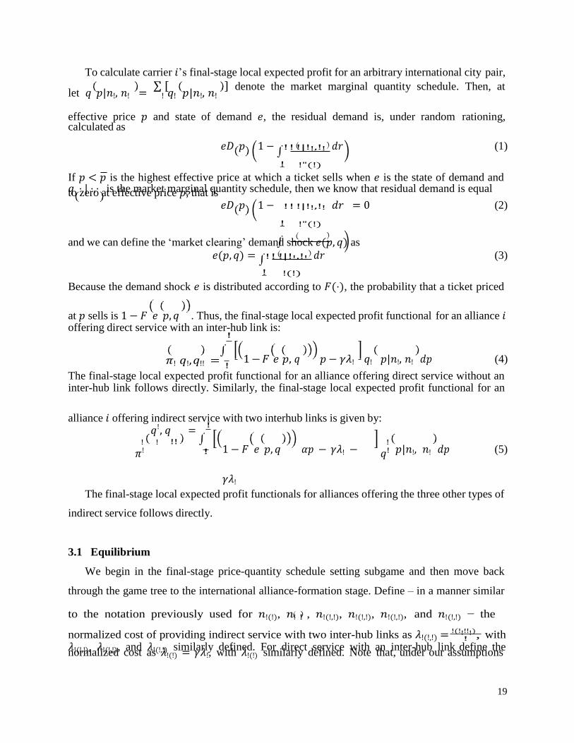
To calculate carrier 𝑖’s final-stage local expected profit for an arbitrary international city pair,

let 𝑞 𝑝|𝑛!, 𝑛! = ! 𝑞! 𝑝|𝑛!, 𝑛! denote the market marginal quantity schedule. Then, at

effective price 𝑝 and state of demand 𝑒, the residual demand is, under random rationing, calculated as

𝑒𝐷 𝑝 1 − ! ! !|!!,!! 𝑑𝑟 (1)

! !"(!)

If 𝑝 < 𝑝 is the highest effective price at which a ticket sells when 𝑒 is the state of demand and 𝑞 ⋅ | ⋅,⋅ is the market marginal quantity schedule, then we know that residual demand is equal to zero at effective price 𝑝, that is

𝑒𝐷 𝑝 1 − ! ! !|!!,!! 𝑑𝑟 = 0 (2)

! !"(!)

and we can define the ‘market clearing’ demand shock 𝑒(𝑝, 𝑞) as

𝑒(𝑝, 𝑞) = ! ! !|!!,!! 𝑑𝑟 (3)

! !(!)

Because the demand shock 𝑒 is distributed according to 𝐹(⋅), the probability that a ticket priced

at 𝑝 sells is 1 − 𝐹 𝑒 𝑝, 𝑞 . Thus, the final-stage local expected profit functional for an alliance 𝑖 offering direct service with an inter-hub link is:

!

𝜋! 𝑞!, 𝑞!! = !

1 − 𝐹 𝑒 𝑝, 𝑞 𝑝 − 𝛾𝜆! 𝑞! 𝑝|𝑛!, 𝑛! 𝑑𝑝 (4)

The final-stage local expected profit functional for an alliance offering direct service without an inter-hub link follows directly. Similarly, the final-stage local expected profit functional for an

alliance 𝑖 offering indirect service with two interhub links is given by:

𝜋!

𝑞!, 𝑞 = !

! 1 − 𝐹 𝑒 𝑝, 𝑞 𝛼𝑝 − 𝛾𝜆! −

𝛾𝜆!

𝑞! 𝑝|𝑛!, 𝑛! 𝑑𝑝 (5)

The final-stage local expected profit functionals for alliances offering the three other types of

indirect service follows directly.

3.1 Equilibrium

We begin in the final-stage price-quantity schedule setting subgame and then move back

through the game tree to the international alliance-formation stage. Define – in a manner similar

to the notation previously used for 𝑛!(!), 𝑛! ! , 𝑛!(!,!), 𝑛!(!,!), 𝑛!(!,!), and 𝑛!(!,!) − the

normalized cost of providing indirect service with two inter-hub links as 𝜆!(!,!) = !(!!!!!), with 𝜆!(!,!), 𝜆!(!,!), and 𝜆!(!,!) similarly defined. For direct service with an inter-hub link define the normalized cost as 𝜆!(!) = 𝛾𝜆!, with 𝜆!(!) similarly defined. Note that, under our assumptions

! !!

20

!

! !

the six normailzed costs are ordered as follows 𝜆!(!) < 𝜆! ! < 𝜆!(!,!) < 𝜆!(!,!) < 𝜆!(!,!) <

𝜆!(!,!). In the statement of Theorem 1, we focus on an arbitrary international city pair and let 𝜆!

denote the normalized cost of the lowest normalized-cost alliance providing service for the city

pair, and let 𝑛! denote the number of alliances offering the lowest normalized-cost service.

Similarly, 𝜆! and 𝑛! denote the normalized cost and number of alliances with the next highest

normalized cost. Starting at the lowest normalized-cost alliance this numbering continues up

until the point that we reach the alliance with the highest normalized cost. For example, if there

exist two alliances offering indirect service with two inter-hub links and two alliances offering

indirect service with no inter-hub links then 𝜆! = 𝜆!(!,!), 𝑛! = 𝑛!(!,!) = 2, 𝜆! = 𝜆!(!,!), and 𝑛! = 𝑛!(!,!) = 2. For any normalized-cost type alliance 𝑗 with 𝑛! > 0, we will refer to type 𝑗 as

being “active” if, in equilibrium, 𝑄! 𝑝|𝑛!, 𝑛! > 0. It will also be convenient to define

𝑦 𝑝 = 1 − 𝐹 𝑒 𝑝, 𝑞 , where 𝑦∗(𝑝|𝑛!, 𝑛!) in Theorem 1 provides the equilibrium probability of making a sale at effective price 𝑝 given the equilibrium total market price-quantity schedule,

𝑞 𝑝|𝑛!, 𝑛! .

3.1.1 Final-Stage Price-Quantity Competition

Theorem 1

21 There exists a unique final-stage local equilibrium that is described as follows.

1) For 𝑛! > 1, let 𝑦∗ 𝑝|𝑛!, 𝑛! be defined over 𝑝 ∈ [𝑝!, 𝑝] as

𝑦∗ 𝑝|𝑛!, 𝑛! = − !!!! ! ! ! !" !

!

!!!!!" !!

!!!! !" ! !!!!

If 𝑛! = 0 or if 𝑦∗ 𝑝|𝑛!, 𝑛! < !! for all 𝑝 ∈ [𝜆!, 𝑝), then the lower bound of the

price support is given by, 𝑝! = 𝑝, where 𝑦∗ 𝑝|𝑛!, 𝑛! = 1. Otherwise,22

for

𝑝 ∈ [𝑝!, 𝑝!), 𝑦∗ 𝑝|𝑛!, 𝑛! is defined as

21 Theorem 1 is stated for the case that 𝐷 𝑝 = 0, if instead the demand function is discontinuous at the choke price

!!

and 𝐷 𝑝 > 0 with D(p)=0 for 𝑝 > 𝑝 then the only change is that an additional term !!

!

!! !

!" ! !!!! is added,

!! !!

!! ! !!!!

because with 𝐷 𝑝 = 0, lim!→! ! !" ! = 0 via L’Hôpital’s rule.

22 That is, n > 0 and there exists a p! > λ! such that 𝑦∗ 𝑝!|𝑛! , 𝑛!

= !!. !! !

21

! ! !!!!(!)

!! ! !

!!! !!

!! ! !

! !!

!

!! 𝑦∗ 𝑝|𝑛!, 𝑛! =

!!

!! ! !!

!" !

! !!! !!

!!! !!!! −

If 𝑛! = 0 or if 𝑦∗ 𝑝|𝑛!, 𝑛! < !! for all 𝑝 ∈ [𝜆!, 𝑝!), then the lower bound of the price support is given by, 𝑝! = 𝑝, where 𝑦∗ 𝑝|𝑛!, 𝑛! = 1. Otherwise,

23this process continues for each 𝑘 = 3, … , 6, where for 𝑝 ∈ [𝑝!, 𝑝!!!),

𝑦∗ 𝑝|𝑛!, 𝑛! is defined as

𝑦∗ 𝑝|𝑛!, 𝑛! =

!!

!!!!

!!!! ! !!!!

!" !

!

!!! !!

!!! !!!! −

and the lower bound of the price support is given by 𝑝! = 𝑝, where

𝑦∗ 𝑝|𝑛!, 𝑛! = 1 if 𝑘 = 6 or if 𝑘 < 6 and 𝑛!!! = 0 or if 𝑘 < 6 and

𝑦∗ 𝑝|𝑛!, 𝑛! <

!!!!

! for all 𝑝 ∈ [𝜆!!!, 𝑝!!!). Otherwise 𝑝! is defined as the

!!!! highest price at which 𝑦∗ 𝑝!|𝑛!, 𝑛! = .

!

2) The case of 𝑛! = 1 is the same as in part 1) except that over 𝑝 ∈ [𝑝!, 𝑝], 𝑦∗ 𝑝|𝑛!, 𝑛! is defined as

𝑦∗ 𝑝|𝑛!, 𝑛! = !!!!(!)

In both cases 1) and 2), for each lowest normalized-cost (i.e., 𝜆!) alliance the equilibrium price-quantity schedule is

𝑞! 𝑝|𝑛!, 𝑛! =

𝑖𝑓 𝑝 ∈ 𝑝!, 𝑝

⋮ −

!!! !!! !!!∗ !

⋮

!!!

𝑛! 𝜆! − 𝜆! 𝑖𝑓 𝑝 ∈ 𝑝! , 𝑝!!!

− 𝑛 𝜆 − 𝜆 𝑖𝑓 𝑝 ∈ [𝑝, 𝑝 )

!!! !!! !!!∗ ! ! ! ! ! !!!

23 That is, n !!! > 0 and there exists a p!

> λ!!! such that 𝑦∗ 𝑝!|𝑛! , 𝑛! = !!!!.

!!

!!! !!!!

!!! !!!!

!!

! ! ! ! !" ! !!! !!!! !"

!

!" !

!!! !

!!! !!!!

!!! !!!!

!!! !!!!

!!!! ! !

! ! !" ! !!! !!!! !"

!

!" !

!!! !

!!! !!!!

! !

!!! !!

!(!)

! !!

! !

!!

!!∗ !

!! !!! !!!∗ !

!!∗ !

!! !!! !!!∗ !

!!∗(!)

!!(!!!(!!!∗(!)))

!

22

!!

!!!!

where, if 𝑛! > 0 and there exists a price 𝑝! ∈ [𝜆!, 𝑝) such that 𝑦∗ 𝑝!|𝑛!, 𝑛! = !!, then 𝑚

denotes the highest “active” normalized-cost type for which 𝑛! > 0 and there exists a price

𝑝!!! such that 𝑦∗ 𝑝!!!|𝑛!, 𝑛! = !! . Otherwise, 𝑝!!! = 𝑝! = 𝑝, and only type 1 alliances

are “active.” For each “active” normalized cost-type 𝑗 = 2, … , 𝑚, the equilibrium price-

quantity schedule is, for 𝑝 ∈ [𝑝, 𝑝!!!]

𝑞! 𝑝|𝑛!, 𝑛! = 𝑞! 𝑝|𝑛!, 𝑛! +

and 𝑞! 𝑝|𝑛!, 𝑛! = 0 for 𝑝 > 𝑝!!!.

𝐷! 𝑝

𝑝𝐹! 𝐹!! 1 − 𝑦∗

𝑝

𝜆! − 𝜆!

The proof that the final-stage local strategy profile specified by Theorem 1 forms an

equilibrium is given in Appendix 1A, and the proof that equilibrium is unique is given in the

Supplemantal Appendix. In solving for the equilibrium price-quantity schedules, note that the

carriers’ best-response functions depend critically on the probability that a ticket with effective

price 𝑝 sells, which is given by 1 − 𝐹 𝑒 𝑝, 𝑞 . This probability depends on the market price-

quantity schedule, 𝑞! 𝑝|𝑛!,!, 𝑛!,! = ! 𝑞!,!(𝑝|𝑛!,!, 𝑛!,!), via the ‘market-clearing’ demand

shock 𝑒 𝑝, 𝑞 . Note also that the lowest normalized-cost flights are offered at all effective prices

𝑝 ∈ [𝑝, 𝑝], while other flights are only offered over, at most, a subset of low effective prices, i.e.,

𝑝 ∈ [𝑝, 𝑝!!!) for “active” normalized-cost type 𝑘.

The 𝑦∗(𝑝|𝑛!, 𝑛!) expression in Theorem 1 provides the probability of making a sale,

1 − 𝐹 𝑒 𝑝, 𝑞 , at effective price 𝑝 given the equilibrium total market price-quantity schedule,

𝑞 𝑝|𝑛!, 𝑛! . Then given the equilibrium probability of making a sale as a function of the price

𝑦∗(𝑝|𝑛!, 𝑛!), the equilibrium price-quantity schedules for each normalized-cost type alliance may be written in terms of 𝑦∗(𝑝|𝑛!, 𝑛!), where 𝑦∗ 𝑝|𝑛!, 𝑛! denotes the equation of motion for

𝑦∗(𝑝|𝑛!, 𝑛!) as the effective price 𝑝 varies over the price support. Because 𝑞 𝑝|𝑛!, 𝑛! is the market marginal quantity schedule, the cumulative market quantity of tickets that are sold at or

!

below an effective price of 𝑝 is given by 𝑄 𝑝|𝑛!, 𝑛! = ! 𝑞(𝑟|𝑛!, 𝑛!)𝑑𝑟.

Thus, the model may be summarized as follows, a demand shock 𝑒 determines the length of the randomly ordered queue of customers with unit demand and heterogeneous reservation

prices, the customers in the queue buy the lowest effectively priced tickets first and then continue

moving up the alliances’ price-quantity schedules until either the demand for or the supply of

23

! !(!,!)

!

tickets is exhausted. If 𝑝 is the highest effective price at which a ticket sells then the total quantity of tickets that are sold in the market is 𝑄 𝑝|𝑛!, 𝑛! . Note that as tickets sell at multiple prices the cumulative market quantity of tickets sold is

determined by the maximum price in the market. However, in matching the theory with the

empirics, it will be convenient to write the market quantity as a function of the average price

instead of the maximum price. Towards that end, let 𝜌(𝑒, 𝑞) denote the maximum price at which a ticket sells – which we henceforth make a slight abuse of terminology and refer to as the ‘market-clearing’ price. This price is a function of both the random length of the queue, (i.e., the

demand shock 𝑒), and the market price-quantity schedule, 𝑞, where 𝜌(𝑒, 𝑞) is implicitly defined by 𝑒 𝜌 𝑒, 𝑞 , 𝑞 = 𝑒. For a given 𝑞 and 𝑒, we have a market clearing price 𝜌(𝑒, 𝑞) which determines the total market quantity of tickets sold 𝑄 𝜌(𝑒, 𝑞) . The market quantity 𝑄 𝜌(𝑒, 𝑞) can then be used to find the average price, which is simply the single price at which the quantity demanded is equal

to the total quantity of tickets sold. That is, 𝑒𝐷 𝑝!"# 𝑄 = 𝑄 𝜌(𝑒, 𝑞) which implies that

𝑝!"#(𝑄) = 𝐷!!

(6)

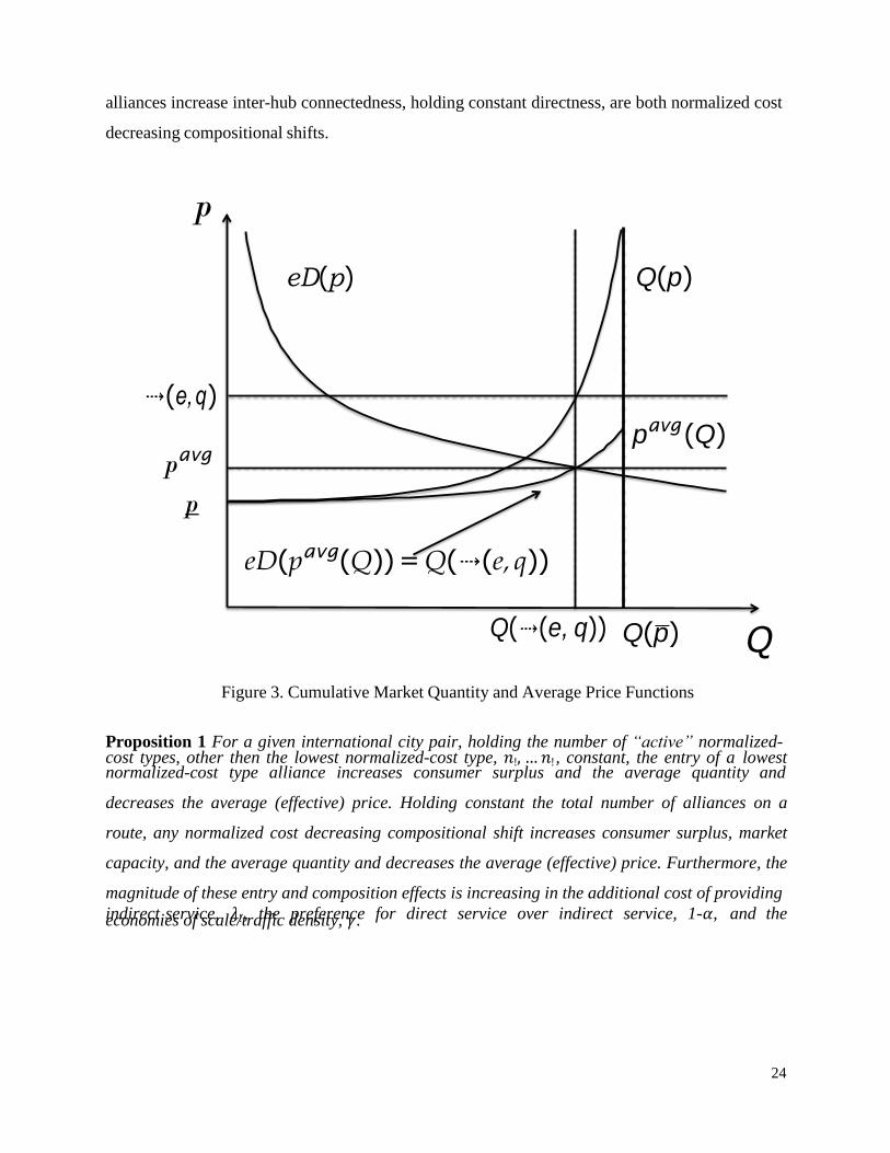
To fix ideas, we graph a particular parameterization24

in Figure 3, which provides the

cumulative market quantity of tickets sold as a function of the maximum price, 𝑄 𝑝 , the average price curve, 𝑝!"# 𝑄 , and the demand curve, 𝑒𝐷 𝑝 , for the state of demand 𝑒. Note that the average price curve, 𝑝!"# 𝑄 , is essentially the market supply curve where the market price is the average price. That is for each demand shock 𝑒, the average price curve identifies that point on the demand curve at which the quantity demanded is equal to the total quantity sold. As

we vary the demand shock, the average price curve traces out those points on the various demand

curves where supply is equal to demand.

We now examine the comparative static results regarding the final-stage local equilibrium

price-quantity schedules, which will feature prominently in the analysis of the first-stage

international alliance formation. Define a normalized cost decreasing compositional shift that

holds constant the total number of alliances on a route as a shift in which for each normalized

cost, one or more alliances move to lower cost types and no alliance moves to a higher cost type.

Note that a shift in which some or all alliances increase directness and shifts in which some or all

24 This parameterization is the special case of CES demand that will be used in the empirical section.

24

alliances increase inter-hub connectedness, holding constant directness, are both normalized cost

decreasing compositional shifts.

p

eD(p) Q(p)

⇢(e, q)

pavg

p

eD(pavg (Q)) = Q(⇢(e, q))

Q(⇢(e, q))

pavg (Q)

Q(p) Q

Figure 3. Cumulative Market Quantity and Average Price Functions

Proposition 1 For a given international city pair, holding the number of “active” normalized- cost types, other then the lowest normalized-cost type, 𝑛!, … 𝑛! , constant, the entry of a lowest normalized-cost type alliance increases consumer surplus and the average quantity and

decreases the average (effective) price. Holding constant the total number of alliances on a

route, any normalized cost decreasing compositional shift increases consumer surplus, market

capacity, and the average quantity and decreases the average (effective) price. Furthermore, the

magnitude of these entry and composition effects is increasing in the additional cost of providing

indirect service, 𝜆! , the preference for direct service over indirect service, 1-𝛼, and the economies of scale/traffic density, 𝛾.

25

The proof of Proposition 1 is contained in Appendix 1B. The key to the proof is that both the

entry and compositional shifts described in Proposition 1 result in an increase in the market price-quantity schedule evaluated at the market clearing price, 𝑄(𝜌(𝑒, 𝑞)), for each demand shock, 𝑒, and, hence, market capacity, 𝑄(𝑝), increases. Recalling the connection between the market price-quantity schedule and the average price curve, 𝑝!"# 𝑄 , it follows that the average quantity rises and the average price falls. As a consequence, consumer surplus rises. Figure 4 illustrates these entry and compositional effects on the average price curve, 𝑝!"# 𝑄 . As can been seen in Figure 4 a rightward shift of the average price curve increases quantities and

decreases prices.

p

Figure 4. Effects of Entry and Compositional Shifts on Average Price Function

From Theorem 1, we know that it may not be profitable for some or all alliances that may

feasibly provide service to be “active” in equilibrium. In that case, an increase in the number of

an “inactive” normalized-cost type has no effect. If, however, it is profitable for more than one

normalized-cost type to offer service, then note that the entry of an alliance that is not of the

lowest normalized-cost type is equivalent to the entry of a lowest normalized-cost type combined

Composi.on "

C " ↵ # #

Entry "

C " ↵ # #

eD(p)

pavg (Q)

Q

26

with a normalized cost increasing compositional shift. As the two components of this sequence

have opposing comparative statics implications, the entry of an alliance that is not of the lowest

normalized-cost type may have an ambigious effect on the equilibrium consumer surplus, market

capacity, average quantity, and average price.

In order to focus on the case that the entry of any alliance, including alliances that are not of

the lowest normalized-cost type, increases consumer surplus, market capacity, and average

quantity, and decreases the average (effective) price, we assume that the difference between the

minimum of the normalized-costs, 𝜆!(!) and the maximum of the normalized-costs 𝜆! !,! is not too large in a sense made formal by the following assumption.

Assumption 1: 𝜆!(!) ≥

!! !,! (!!!!!!!)

!!!!!

The following proposition, the proof of which is contained in Appendix 1B, establishes that

Assumption 1 provides a sufficient condition for the existence of unambigous comparative

statics predictions given the entry of any normalized-cost type alliance.

Proposition 2 Under Assumption 1, for a given international city pair, the entry of any

normalized-cost type alliance increases consumer surplus, market capacity, and the average

quantity and decreases the average (effective) price. Furthermore, the magnitude of this effect is

increasing in the additional cost of providing indirect service, 𝜆! , the preference for direct service over indirect service, 1-𝛼, and the economies of scale/traffic density, 𝛾.

Although we have not explicitly modeled it here, our model can be extended to allow for

exogenous pre-OSA capacity constraints on international travel between gateway cities. In

equilibrium, a binding capacity constraint creates a shadow cost of capacity that implicitly

increases the capacity costs. As the equilibrium average price function is decreasing in these

capacity costs, a binding capacity constraint results in lower quantities and higher average prices.

3.1.2 First-Stage International Alliance Formation

We now move back through the game tree to first-stage international alliance formation. In

the shift from the pre-OSA to post-OSA environment there are two key changes: (i) the

restriction on the set of “international gateway” cities into which carriers may fly is removed and

.

27

(ii) cooperative agreements including codeshares and alliances between domestic and foreign

carriers are allowed.

It is useful to begin by examing the effect of only elminating route restrictions (without

allowing alliances) in our model. Note that in the absence of international alliances, no carrier’s

most direct post-OSA feasible service features an inter-hub connection. For an arbitrary

international city pair that includes a non-gateway city 𝑗, the total number of carriers that may

feasibly provide direct service, post-OSA, for this city pair is equal to the total number of

domestic carriers that have a hub at the non-gateway city, 𝛤! ,25

plus the one foreign carrier with

a hub at the foreign gateway city in the city pair. From Proposition 1, it follows that both the

entrance of the foreign carrier – which was unable to provide indirect service pre-OSA – and the

compositional shift of the domestic carriers with hubs at the non-gateway city from indirect

service to direct service increases consumer surplus, market capacity, and the average quantity

and decreases the average (effective) price.

Post-OSA indirect carriers may or may not be active, but all 𝑛! − 𝛤! domestic carriers without a hub at non-gateway city 𝑗 may continue to provide indirect service via one of their gateway hubs in country 𝐴.

26 In addition, all 𝑛! − 1 foreign carriers without a feasible direct

connection may now enter and provide indirect service via their foreign gateway. Under

Assumption 1, we know from Proposition 2 that the entry of any normalized-cost type alliance

increases consumer surplus, market capacity, and the average quantity and decreases the average

(effective) price. Thus, the removal of route restrictions provides unambiguous gains for

consumers. Note, however, that allowing for alliances introduces two features with confounding

comparative static effects, a decrease in the number of players in the final-stage game and inter-

hub connections that lower costs.

Recall that Pre-OSA alliance formation is not possible and each carrier is an alliance of one,

and that post-OSA alliance formation endogenously takes place in a sequential-move bargaining

with binding commitments environment. It follows from Ray and Vohra (1996) that in the post-

OSA alliance formation game there exists a Markov perfect equilibrium of the first-stage

international alliance-formation game, where the state of the game is given by the set of alliances

that have already formed and retired from the game.

25 Where 𝛤! denotes the cardinality of the set 𝛤! .

26 Recall that each domestic carrier has at least one gateway hub.

28

Proposition 3 [Ray and Vohra 1999, Theorem 2.1] There exists a Markov-perfect equilibrium of

the international alliance-formation game.

Given the existence of a first-stage equilibrium, we now examine the effects of OSA

agreements as we move from the pre-OSA environment to any equilibrium alliance partition in

the post-OSA environment. We begin with the case of an arbitrary international city pair that

includes a non-gateway city 𝑗, then examine the case of a pair of international gateway cities, and conclude with the case that OSAs are introduced in some but not all foreign countries.

For international city pairs involving non-gatway cities, post-OSA it follows from the distinct

country restriction on the set of possible partitions of carriers into alliances that for each

domestic carrier there is at least one post-OSA alliance that may feasibly provide service with a

normalized cost that is at least as low as pre-OSA. In addition, there may be an increase in the

number of alliances that may feasibly provide service for the city pair.27

Proposition 4 In moving from the pre-OSA to post-OSA environment, for any equilibrium of the

alliance formation game it is the case that for city pairs involving non-gateway hubs average

directness and interhub connectedness increase and the equilibrium consumer surplus, market

capacity, and average quantity increase while the average (effective) price decreases.

Given that for any post-OSA equilibrium of the alliance formation game, the pre- to post-

OSA transition is characterized by a normalized cost decreasing compositional shift and/or entry,

Proposition 4 follows from Propositions 1 and 2.

For an arbitrary pair of international gateway cities, note that elminating route restrictions, in

the absence of international alliances, has no effect. As before, in this scenario no carrier’s most

direct post-OSA feasible service features an inter-hub connection. For an arbitrary gateway-

gateway city pair, all domestic carriers with a hub at domestic gateway city 𝑗, 𝛤! , and the one foreign carrier with a hub at the foreign gateway may, both pre- and post-OSA, feasibly provide direct international service for the city pair. Similarly, for indirect service, the remaining

𝑛! + 𝑛! − 𝛤! − 1 domestic and foreign carriers may, both pre- and post-OSA, feasibly provide

27 For example, this would arise if the foreign carrier with the hub at the foreign gateway in the city pair does not

form an alliance with a domestic carrier.

29

international service for the city pair. Thus, the removal of route restrictions has no effect on

consumers.

As noted before, alliance formation leads to a decrease in the number of players in the final-

stage game but, also, creates inter-hub connections that lower costs. In the case of an

international city pair involving a non-gateway city, the removal of route restrictions outweighed

the ambiguous alliance effects and led to consumer gains. But, because the removal of route

restrictions has no effect for a pair of international gateway cities, we are left with only the

ambiguous alliance effect. Thus, we cannot eliminate the theoretical possibility that for a pair of

international gateway cities the introduction of OSAs may potentially lead to a type of Braess’

paradox problem in which total consumer surplus decreases as route restrictions are removed and

alliances are allowed to form.

We conclude the analysis of first-stage international alliance formation by examining the

case that OSAs are introduced in some but not all foreign countries.

Proposition 5 In moving from the pre-OSA to post-OSA environment, for any equilibrium of the

alliance formation game it is the case that at the gateways of foreign countries where OSAs are

not introduced average directness and interhub connectedness increase and the equilibrium

consumer surplus, market capacity, and average quantity increase while the average (effective)

price decreases.

Proposition 5 follows from lines similar to Proposition 4. In particular, despite the fact that

foreign carriers in countries where OSAs are not introduced face the same route restrictions, the

foreign carriers in neighboring countries where OSAs are introduced may now, via their

country’s gateway, offer indirect service between any non-gateway hub in country A and the

non-OSA foreign countries. As was the case with Proposition 4, it follows from the distinct

country restriction on the set of possible partitions of carriers into alliances that for each

domestic carrier there is at least one post-OSA alliance that may feasibly provide service that is

at least as direct and is at least as inter-hub connected. There may also be an increase in the

number of alliances that may feasibly provide service for the city pair. Thus, the result for

service between non-gateway routes and non-OSA foreign gateways follows directly. Note

however, that unlike the case of countries where OSAs are introduced, in non-OSA countries

service on gateway-to-gateway routes experience unambiguous gains. This arises because: (i) the

30

introduction of OSAs in neighboring countries allows for new indirect routes, and (ii) the

inability of the carrier in the non-OSA country to join an alliance means that the number of

alliances that may feasibly provide direct gateway-to-gateway service to the non-OSA country

does not decrease. Thus, OSAs create a positive externality for non-OSA countries.

4. Data Sources and Description

We draw on two rich datasets that cover international travel to and from the United States at

quarterly frequencies over the period 1993-2008. The Databank 1B (DB1B) Origin and

Destination Passenger Survey represents a 10 percent sample of airline tickets drawn from

airport-pair routes with at least one end-point in the U.S. Each airline ticket purchase recorded in

the data contains information on the complete trip itinerary including airports, air carriers

marketing the ticket and operating each flight segment, the total air fare, distance traveled split

by flight segments, ticket class type, as well as other segment level flight characteristics. We

focus on U.S. outbound economy-class tickets, and restrict attention to foreign countries with at

least one city-pair route serviced continuously over the time period.

One limitation of the DB1B data is that the foreign carriers that are not part of immunity

alliances are not required to file ticket sales information to the U.S. Department of

Transportation.28

However, this is less of an issue for U.S. outbound tickets as compared to

inbound ones. Tickets whose first segment originates in the U.S. are more likely to be sold by

U.S. carriers and therefore appear in the data. We employ some additional filters to prepare the

data sample, which are described in the Data Appendix. The resulting sample includes 40,376

origin-destination airport pairs, with an average of 13 observations per pair. The summary

statistics for the variables of interest are provided in the Appendix Table A3.

We augment the empirical analysis with an alternative dataset that offers complete coverage

of all U.S. international passenger traffic. The T100 International Segment database provides

information on capacity and air traffic volumes on all U.S. non-stop international flight segments

(defined at airport-pair level), distinguished by the direction of travel, and operated by both

domestic and foreign carriers. The data is collected at monthly frequencies and reports for each

carrier-route pair the number of departures scheduled and operated, seats supplied, onboard

28 Immunity alliances represent strategic alliances between domestic and foreign airlines with granted antitrust

immunity from the U.S. Department of Transportation. Immunity grants allow carriers to behave as if they were

merged, cooperating in setting prices and capacity on all joint international routes to and from the U.S.

31

passengers, segment distance and airborne time.29

The disadvantage to the T-100 data is two-

fold. They do not include pricing information, and they do not provide details on complete

origin-destination itineraries, but rather report only the flight segments that cross the US border.

Accordingly, the T100 data are best for describing changes in total passengers exiting the

US, the number of distinct exit points out of the US, and the capacity allocated to those exit

points. This makes it ideal for evaluating model mechanisms related to route restrictions and

capacity reallocation. The DB1B data are best suited for describing prices and routing structures,

especially for indirect tickets, for true origin-destination city pairs. This makes it ideally suited

for evaluating changes in consumer welfare.

Table 1 summarizes regional growth in passenger traffic on non-stop segments, and regional

growth in the share of traffic covered by OSAs, during the sample period 1993-2008. Figure 1

shows the annual time series aggregated over regions. By any measure of industry performance −

passenger volumes, number of non-stop international routes or annual departures performed

(unreported) − international air traffic has grown rapidly during this period of deregulation. By

2007, 59 percent of the total U.S. international air passenger traffic passed through a foreign

gateway airport located in an Open Skies country.

5. Econometric Analysis

We examine how international passenger aviation changes in the wake of trade liberalization

efforts, focusing on change along three dimensions. First, we use a difference in difference

methodology to compare growth in passenger traffic pre/post liberalization to growth in the same

period for non-liberalization countries. Second, we decompose aggregate changes into growth in

traffic along “new” and existing routes, and also evaluate reallocations of carrier capacity across

routes. The decompositions provide insight into key model mechanisms and the role of route

restrictions in pre-OSA regulation. Third, we estimate the partial effects of liberalization on the

price, quantity and quality (directness) of passenger aviation, and examine whether these effects

are asymmetric across gateway and non-gateway cities, as predicted by the theory. Finally, we

combine these estimates to calculate the total change in (quality-adjusted) prices after OSAs in

order to assess the consumer welfare gains from air services liberalization.

29 However, the T100 Segment data does not easily match to the true Origin and Destination Passenger data, since

passengers with very different start and end point itineraries get lumped together in a single observation in the T100

Segment dataset if their cross-border flight segment is the same. Unlike goods, which feature a one-to-one relation

between a product and its producer, international air travel often involves the service of more than one airline. This

is why firm- and product-level air travel datasets are imperfectly compatible.

32

d,93

5.1 Growth of Passengers and Routes: T100 Data

We begin by examining traffic growth using the T-100 International segment data. We

observe passenger traffic for every carrier and every city-pair route. Total air passenger traffic

between the United States and destination country d at time t is the sum of traffic across all non-

stop origin-destination routes and carriers offering service. We will also distinguish between

growth along existing routes (i.e., intensive margin) versus newly introduced routes (i.e.,

extensive margin).

We use two ways to decompose the total U.S. outbound traffic to country d, Qdt, into an

intensive and extensive margin. The simplest approach is to count the number of direct

connection city-pair aviation routes offered at a given point in time, Ndt, and then determine the

average passenger volume per route:

𝑄!" = ! 𝑄!"# = 𝑁!" ∗ 𝑄!" (14)

A drawback of this ‘simple count’ approach is that it treats all air services as having equal

value weights in the total consumption of international travel. Alternatively, we can weight the

importance of existing routes using information on (lagged) passengers in a manner similar to the

“new variety” literature following Feenstra (1994). In this second calculation, we define the

intensive margin for destination country d as the volume of air traffic on aviation routes that are

available in both the current and a three-year lag reference period. We also define the extensive

margin as being the passenger-share weighted count of aviation routes that are “new” relative to

the reference period. The details on the construction of the passenger-weighted decomposition is

relegated to the Econometric Methodology Appendix 2A.

We normalize the level of each variable obtained from the decomposition by its value in the

base year to get an expression for the cumulative air traffic growth during our sample:

!" !" !" !" !" !!"

∆𝑄!" = ∆𝐼𝑀!" ∗

∆𝐸𝑀!"

where ∆𝑍!" = !!!""# ! !"!!

(15)

with Z {Q, IM, EM}. We set Z93

to one.

To estimate the impact of liberalization on air passenger transport, we rely on the time series

dimension of the T100 International Segment data. Our identification strategy compares the

change in passenger volumes within a country pair before and after the introduction of the Open

Skies Agreements with the corresponding value calculated for countries that maintain restrictive

33

aviation policies (control group). In using this difference-in-difference estimation method we

consider the following regression model:

34

!" ! !" !"

𝑙𝑛∆𝑍!"# = 𝛽!𝑂𝑆𝐴 + 𝛽!𝑙𝑛∆(!) !"# + 𝛽!𝑙𝑛∆𝐿!"# + 𝑋𝛽 + 𝛼!" + 𝛼! + 휀!"# (16)

where d, q and t index the country, quarter and year respectively, and Z {Qdqt, IMdqt, EMdqt}

takes in turn each variable, expressed as cumulative growth. The variable of interest OSAdqt is an

indicator variable that equals 1 for all the years when an Open Skies Agreement exists between

the U.S. and country d. We also control for per capita income Y/L, and population L of

destination country d. X denotes a vector of additional control variables, including Partial

Liberalization (an indicator for non-OSA countries with more relaxed air transport agreements),

a 9/11 control variable, and its interaction with a Visa Waiver Program (VWP) indicator to

capture any differential response to the tightened security post 9/11 (Neiman and Swagel

2009)30

. We also include selected region and country trend variables, and country-season (e.g.

travel to Mexico is greater in the 4th

quarter than in the 2nd

and both are higher than any quarter

of travel to Ghana) and year fixed effects. Since all our data involve US bilateral flows, the year

effects eliminate any time-varying changes that are common to all routes, including changes in

input prices or technology, or secular change in aviation demand.

Endogeneity of Open Skies Agreements

One complication in policy evaluation comes from the potential endogeneity between the

change in policy and the outcome variable(s) of interest. In our case, a primary concern is that

some omitted variable affects the scale or expected future growth of aviation traffic with country

d and this omitted variable is correlated with the likelihood and/or timing of an Open Skies

Agreement. Countries differ substantially in size and income, the quality of aviation

infrastructure, the dependence on aviation for trade, migration, or tourism, and the strength or

political connections of their domestic airlines. The US may be more likely to sign agreements,

or sign them earlier, when the benefits of signing are greater and the political opposition to

signing is less.

This problem is likely to be most severe in the cross-section, as there are a host of difficult to

control for reasons why Germany and Ghana differ in the structure of their aviation markets and

the returns to agreements. Many studies of services liberalization are limited to cross-section

30 Very few countries change Visa Waiver Program Status during our sample period, so including the VWP variable

independently in the regression has no effect on the estimates.

35

data, but we are able to we exploit our 16 year panel and employ country fixed effects to exploit

only within country time series variation pre/post signing. (In regressions using DB1B data we

employ even more stringent city-pair fixed effects.) Taking a step further, countries that sign

agreements at some point may be fundamentally different than countries that do not sign

agreements at any point. Here, we can exploit our long time series and the fact that 108 countries

have signed OSAs spread over the 1992-2013 period. In most of our regressions we restrict our

samples to only those countries that sign agreements at some point and exploit only differences

in the timing of when agreements are signed. Note that our T100 and DB1b data samples end in

2008, so there are 21 eventual signers of OSAs included in our sample for whom the OSA

“treatment” will be outside the sample.

This leaves the endogeneity of timing itself. As an initial look at this problem, we inspect the

timing of agreements provided in appendix Table A1. What we see is that there is no clear

pattern to the timing of the agreements. After The Netherlands signs the first agreement in 1992,

8 OECD European countries sign in 1995. But the rest of Europe is spread throughout the

sample, with one each in 1996, 1998, 1999, 2001, and then a final group in 2007. Many Latin

American countries sign in 1997, and other signings occur over the next 8 years. Similar partners

are found for East Asia, South Asia, Central Europe, and Africa. Table 1 has the percentage of its

region that signs at each of three points in time, and again there is no clear pattern. By the end of

the period, all of OECD Europe is in, but other regions all have a mix of signers and non-signers.

Appendix Table A2 examines the timing of signing and its correlates, including levels and

growth rates of population, GDP, GDP per capita, exports, distance, and tariffs. None are

statistically significant (though if we enter a “high income” indicator with no other controls it is

marginally significant). We also explored characteristics of air traffic routes prior to signing

agreements including the country’s number of departures worldwide, carrier concentration on

routes, and the restrictiveness of existing agreements, including whether they included

restrictions on routes, carriers, price setting, or capacity restrictions. Of these, only the existence

of capacity restrictions is correlated with early signing, and so we include the degree of partial

liberalization as a control in the regressions.31

31 We have explored similar regressions in which the dependent variable is binary (sign/don’t sign), a source of

variation that is taken out of the regression when we use samples of only signatories. Nevertheless even sign/don’t

sign shows similar lack of correlation, with the exception of a weak positive correlation with per capita income,

driven by OECD Europe. It appears that there is no obvious pattern to which countries sign agreements.

36

A final possibility is that there are changes in growth rates that happen to coincide with

signing OSAs. To rule this out we interact the OSA dummy with a vector of time dummies

corresponding to t-4 through t+5, where t is the date of signing. This enables us to see whether

aviation traffic was already growing prior to the OSA signing or whether changes in growth rates

correspond to the date agreements were signed. We return to this point in the results discussion

below.

Estimation Results

Panel A of Table 2 reports the regression model in equation (16) estimated using the

cumulative growth decomposition in equation (15). In Column 1 we see that countries who

liberalize their international aviation markets experience a 7.1 percent increase in passenger

traffic. The increase in aggregate volumes is explained in part by the net expansion of

international aviation routes. Countries that sign OSAs see 10.5 percent faster growth in the

number of routes, as measured by a simple count (Column 2). When using weighted counts

(Column 4) liberalization increases the extensive margin of passenger growth by 3.9 percent.

The difference in the weighted and un-weighted estimates indicates that new routes, on average,

are opened in smaller cities with fewer passengers.

Liberalization also affects the cumulative passenger growth along routes previously offered,

though the intensive margin effect is imprecisely estimated in both specifications. Given the log-

additive property of the components of the air traffic decomposition, the coefficients on OSA in

the total traffic regression will be equal to the coefficients from the extensive and intensive

margin regressions, respectively. We can then say that the extensive margin accounts for

(3.9/7.1)=55 percent of overall growth in the weighted regression, and (10.5/7.1)=148 percent of

overall growth in the simple count regressions.

The simple OSA indicator specification assumes that there is a one-time level change in

growth rates after signing. But aviation markets may take time to adjust to new policies, as

carriers experiment with new markets and route networks, and consumers learn of new

opportunities. To account for this we interact the OSA indicator with a vector of time dummies

corresponding to t-1 through t+5, where t is the date of signing. This enables us to see whether

increases in traffic growth accumulate over time.

Panel B of Table 2 reports the regression results. Two points emerge from these estimates.

First, for all three dependent variables, the impact of air services liberalization increases

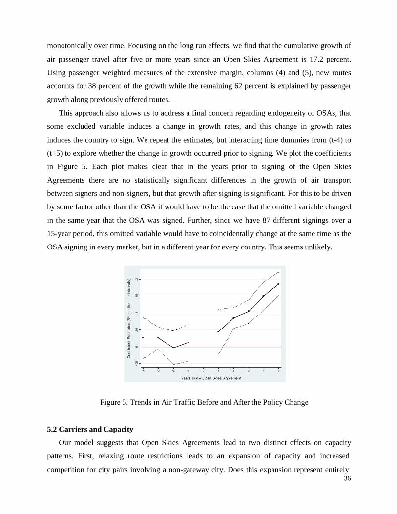
36

monotonically over time. Focusing on the long run effects, we find that the cumulative growth of

air passenger travel after five or more years since an Open Skies Agreement is 17.2 percent.

Using passenger weighted measures of the extensive margin, columns (4) and (5), new routes

accounts for 38 percent of the growth while the remaining 62 percent is explained by passenger

growth along previously offered routes.

This approach also allows us to address a final concern regarding endogeneity of OSAs, that

some excluded variable induces a change in growth rates, and this change in growth rates

induces the country to sign. We repeat the estimates, but interacting time dummies from (t-4) to

(t+5) to explore whether the change in growth occurred prior to signing. We plot the coefficients

in Figure 5. Each plot makes clear that in the years prior to signing of the Open Skies

Agreements there are no statistically significant differences in the growth of air transport

between signers and non-signers, but that growth after signing is significant. For this to be driven

by some factor other than the OSA it would have to be the case that the omitted variable changed

in the same year that the OSA was signed. Further, since we have 87 different signings over a

15-year period, this omitted variable would have to coincidentally change at the same time as the

OSA signing in every market, but in a different year for every country. This seems unlikely.

Figure 5. Trends in Air Traffic Before and After the Policy Change

5.2 Carriers and Capacity

Our model suggests that Open Skies Agreements lead to two distinct effects on capacity

patterns. First, relaxing route restrictions leads to an expansion of capacity and increased

competition for city pairs involving a non-gateway city. Does this expansion represent entirely

37

new activity or is it a reallocation of capacity and competition away from pre-OSA gateways to

the new routes? Because pre-OSA domestic carriers were forced to route their indirect service

from non-gateway hubs through a domestic gateway, post-OSA carriers may, subject to

feasibility, offer direct service on such routes and reduce the capacity allocated to the service of

indirect passengers via gateway city pairs. In addition, the introduction of alliances may decrease

competition on gateway city pairs to the point that, despite the cost savings created by alliances,

the capacity allocated to the service of gateway-to-gateway passengers decreases.

We examine these conjectures in the last two columns of Table 2 and in Figure 6. In Table 2

we measure capacity (total seats offered between the US and country d), and the share of pre-

OSA gateways in total seats. (Multiplying these measures together gives the number of seats

offered on pre-OSA gateways; adding the coefficients gives the change in those seats after

OSAs.) In panel A we see that the average effect is a 5.4 percent rise in total capacity post-OSA

and a 6.4 percent reduction in the share of pre-OSA gateways. This implies that not only did

capacity outside the gateways rise, but also capacity on the gateways fell.

In Panel B we interact the OSA variable with a vector of time dummies to see transition and

long run effects. Five years after signing, post-OSA capacity rises by 16 percent, and the share of

pre-OSA gateways falls by 13 percent. If we compare the share of capacity on the gateways one

year prior to the OSA to five years after, we see a decline on of 19 percent (relative to the

country and time fixed effects). Relaxing restrictions both increases aggregate capacity and shifts

it significantly away from the gateways.

In Figure 6 we examine whether this route reallocation also changed the number of

competitors on different routes. We begin by counting the number of carriers competing on each

origin-destination route at a point in time, and organizing these into 4 equal size bins from fewest

competitors (at left) to most competitors. We then examine the change in the number of carriers

over the subsequent two years. This is represented by the vertical bars in Figure 6, and

distinguish between routes that experience a change in the aviation policy during the two year

span (i.e., a switch in the OSA indicator from 0 to 1), versus routes that do not experience such a

change.

Routes with the fewest carriers see the most entry, and routes with the most carriers see exits.

More importantly for our purposes, these patterns of entry and exit are more accentuated on

routes that experience liberalization of air services. For the routes with the fewest carriers, the

average rate of entry is 22 percent higher for markets going through a liberalization process,

38

while for the routes with the largest number of carriers, the average rate of exit is 25 percent

higher. This is consistent with the view from the model that existing regulations force an

“excess” allocation of capacity to a few gateway cities. These gateways enjoy intense

competition, while remaining routes have few competitors. Post-OSA, not only is there entry on

the off-gateway routes, but the ability to form alliances results in a decrease in competition on

the gateways. The unregulated market results in a different, and less concentrated, distribution

of both capacity and competition.

Notes: The number of carriers per cross-border flight segment is calculated based on simple count using T100 Data. Each origin-destination-time observation is assigned to one of the four an equal-sized bins based on the number of carriers in the market, with bin 1 including the least competitive routes. The vertical bars measure the change in carriers over a 2-year period for a given route, averaged across all routes in the respective bin. Within each bin, we distinguish between routes that went through liberalization.

Figure 6. Air Carrier Entry and Exit Across Routes

5.3 Price, Quantity and Quality Effects of Open Skies Agreements

Our model suggests several ways in which OSAs could affect prices, quantities and qualities.

On non-gateway hubs, the introduction of more direct routes reduces the marginal cost of

providing service and provides quality gains for consumers who value directness, and the

formation of alliances lowers marginal costs by increasing inter-hub connectedness. On

gateways, relaxed capacity constraints could lower average prices though this effect competes

with the reallocation of capacity toward newly unrestricted routes and the ambiguous effects of

alliance formation.

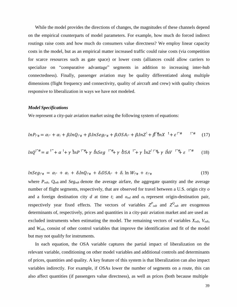
39

!"# ! !"# !"#

!"# !" ! ! !"# ! !"# ! !" ! !"# ! !"# !"#

While the model provides the directions of changes, the magnitudes of these channels depend

on the empirical counterparts of model parameters. For example, how much do forced indirect

routings raise costs and how much do consumers value directness? We employ linear capacity

costs in the model, but as an empirical matter increased traffic could raise costs (via competition

for scarce resources such as gate space) or lower costs (alliances could allow carriers to

specialize on “comparative advantage” segments in addition to increasing inter-hub

connectedness). Finally, passenger aviation may be quality differentiated along multiple

dimensions (flight frequency and connectivity, quality of aircraft and crew) with quality choices

responsive to liberalization in ways we have not modeled.

Model Specifications

We represent a city-pair aviation market using the following system of equations:

𝑙𝑛𝑃!"# = 𝛼!" + 𝛼! + 𝛽!𝑙𝑛𝑄!"# + 𝛽!𝑙𝑛𝑆𝑒𝑔!"# + 𝛽!𝑂𝑆𝐴!" + 𝛽!𝑙𝑛𝑍! + 𝛽 𝑙𝑛𝑋 + 휀 (17)

𝑙𝑛𝑄 = 𝛼 + 𝛼 + 𝛾 𝑙𝑛𝑃 + 𝛾 𝑙𝑛𝑆𝑒𝑔 + 𝛾 𝑂𝑆𝐴 + 𝛾 𝑙𝑛𝑍! + 𝛾 𝑙𝑛𝑉 + 휀 (18)

𝑙𝑛𝑆𝑒𝑔!"# = 𝛼!" + 𝛼! + 𝛿!𝑙𝑛𝑄!"# + 𝛿!𝑂𝑆𝐴!" + 𝛿! ln 𝑊!"# + 휀!"# (19)

where Podt, Qodt and Segodt denote the average airfare, the aggregate quantity and the average

number of flight segments, respectively, that are observed for travel between a U.S. origin city o

and a foreign destination city d at time t; and αod and αt represent origin-destination pair,

respectively year fixed effects. The vectors of variables ZP

odt and ZQ

odt are exogenous

determinants of, respectively, prices and quantities in a city-pair aviation market and are used as

excluded instruments when estimating the model. The remaining vectors of variables Xodt, Vodt,

and Wodt, consist of other control variables that improve the identification and fit of the model

but may not qualify for instruments.

In each equation, the OSA variable captures the partial impact of liberalization on the

relevant variable, conditioning on other model variables and additional controls and determinants

of prices, quantities and quality. A key feature of this system is that liberalization can also impact

variables indirectly. For example, if OSAs lower the number of segments on a route, this can

also affect quantities (if passengers value directness), as well as prices (both because multiple

40

segments directly impact costs, and through a quantity channel if costs are not linear in

quantities). To properly estimate these effects we incorporate a set of additional controls that

include the instruments necessary to trace out exogenous variation in each right hand side

variable. These instruments are discussed in depth below.

We focus initially on mapping these equations into the model. In the pricing equation (17),

the dependence of average prices on the number of segments corresponds to the assumption that,

c.p., indirect routes increase costs. In the model we assume that capacity costs are linear, which

would imply a coefficient of zero on quantities. Here we allow the more general case that

(exogenous) changes in passenger quantities affect prices. Note that there is a critical difference

between exogenous (and predictable) changes in passenger demand and the random demand

shocks described in the model. The latter generate a strong positive correlation between average

prices and quantities ex-post but this effect will be purged from the estimation by instrumenting

for demand.

For simplicity, the model focuses on heterogeneity arising from direct vs. indirect service and

the inter-hub connections generated by alliances. Here we also allow for costs to differ across

routes and time periods. Most of these differences are captured by origin-destination and time

fixed effects. In addition, some inputs vary across time and geography in a way that is useful for

identifying changes in costs. For example, takeoff/landing intensively uses fuel, so fuel

represents a larger percentage of costs on short haul flights. Changes in fuel costs over time will

then represent a larger percentage change for short versus medium length flights. Accordingly,

we use interactions of fuel costs with flight distance (direct distance, its square, and excess

distance traveled) to construct the exogenous vector of instruments ZP

odt. Additional control

variables included in the vector Xodt in equation (19) are: aircraft insurance costs (which changed

markedly in this period) interacted with indicators for main world geographic regions, and per

capita incomes for origin and destination cities to account for differences in consumers’

willingness to pay for flights.

In the demand equation (18), the dependence of quantities on (exogenous) changes in

average prices captures the slope of the demand curve. The effect of (exogenous) changes in the

number of segments represents an outward shift of the demand curve and reflects consumer’s

valuation of more direct flights. These two variables account for the channels explicitly

developed in the model while the OSA variable captures additional changes in quantity

demanded conditional on price and number of segments. As such it captures changes in implicit

41

quality of flights after OSA signing. The vector ZQ

odt controls for demand determinants that

influence the number of passengers traveling in an o-d market. It consists of the city population

and per-capita income at origin and destination.

Finally, the average number of segments, equation (19), depends on (exogenous) changes

in passenger traffic and the OSA variable. Here, the OSA variable captures the relaxation of

gateway restrictions. Apart from these effects, the number of segments is largely a function of

geography (o-d fixed effect), but the cost of employing multiple takeoff/landings varies over

time as a function of fuel prices. Like the average price regression we employ fuel prices

interacted with direct and excess distances traveled on multiple segment routes. The vector Wodt

of control variables for the average number of flight segments (equation 19) accounts for the

purchasing power of consumers at both origin and destination. Conditional on the volume of air

traffic within the city pair market, higher levels of their per-capita income increase the directness

of the air services provided.

Policy Variable

The main variable of interest is OSAdt. In its simplest form, it is defined as a dummy variable

equal to one for all the years since the signing of an Open Skies Agreement by the country to

which destination city d belongs. However, the networked nature of international passenger

aviation means that a passenger in a non-signatory country can still benefit from OSAs signed by

neighboring countries. Similarly, signing an agreement may have a smaller effect on market

outcomes if neighbors have already signed. Ignoring these indirect OSA effects may bias the

estimates by ‘contaminating’ the reference group of fully regulated air travel flows, thus making

it difficult to identify the actual effect of air services liberalization.

To account for this issue, we construct an OSA variable that takes into account the extent to

which passengers route through other OSA hubs in the periods prior to liberalization. We first

calculate the passenger share within an origin-destination market that transit through third

country OSA hubs on the way to their final destination. !!"#$

𝑂𝑆𝐴 𝑃𝑎𝑥 𝐶𝑜𝑛𝑛𝑒𝑐𝑡!"

=

!!"# ∗ 𝐼(𝑂𝑆𝐴!! =

1)

(20)

where i denotes a city hub located in a country different from the final destination country when

travelers connect flights when traveling from origin o to destination d; and I(.) is an indicator

function.

!

42

We define another similar OSA Connect variable that also takes into account the fraction of

the trip distance traveled along flight segments covered by Open Skies Agreements:

𝑂𝑆𝐴 𝐷𝑖𝑠𝑡 𝐶𝑜𝑛𝑛𝑒𝑐𝑡!"

=

!!"#$

! !!"#

∗ !"#$!"#

!"#$!"# ∗ 𝐼(𝑂𝑆𝐴!" =

1)

(21)

The regression variable used in the main estimation exercises combines information about

the OSA signing by the final destination country with the previously defined OSA Connect

variables, as follows:

𝑂𝑆𝐴 𝐶𝑜𝑚𝑏𝑖𝑛𝑒!"

=

1 𝑖𝑓 𝑂𝑆𝐴!" = 1 1 𝑖𝑓 𝑂𝑆𝐴!" = 0 𝑎𝑛𝑑 𝑂𝑆𝐴 𝐶𝑜𝑛𝑛𝑒𝑐𝑡!" > 𝑘

0 𝑜𝑡ℎ𝑒𝑟𝑤𝑖𝑠𝑒

(22)

where k is a threshold value such as the median or the 25th

percentile, and OSA Connect is

measured either as a passenger share, or as a distance share.

Model Identification

The regression equations (17), (18) and (19) represent our main estimation models. Given the

use of time and market-specific fixed effects, the identification of each model relies entirely on

time variation within each origin-destination city pair. The main empirical challenge comes from

the interrelation between the three dependent variables, giving rise to endogeneity concerns. To

address this endogeneity problem, we estimate each of the three equations using the instrumental

variables method and rely on exogenous instruments suggested either by the other regression

equations, or by mechanisms external to the model.

For example, in the model the (ex-post) average price and aggregate quantity are

simultaneously determined as a function of demand shocks. In the pricing equation we

instrument for quantity using population size at origin and destination, and add two external

instruments: the volume of U.S. state level exports to the final destination country, as well as an

indicator for participation in the Visa Waiver Program. These latter excluded variables are also

used to instrument for quantity in the flight segment regression.32

43

In the quantity regression we instrument for both the price level and for the number of

segments. The natural candidates are input costs, particularly distance-related cost variables,

32 We do not include population at origin and destination as instruments for quantity in the flight segment regression

for lack of certainty about their excludability from the regression model. However, adding them to the list of

exogenous instruments does not change the estimation results. Results are available upon request.

44

since they are correlated both with prices but also the route structure through landing/take-off

expenses. Therefore, we propose three exogenous instruments: 1) the non-stop distance between

the origin and destination cities interacted with fuel prices; 2) the excess travel distance

calculated in the base year as the ratio of the average ticket distance (determined by connections)

to the non-stop distance, which again we interact with fuel prices; and 3) the excess distance

squared interacted with fuel prices. One important thing to notice about the proposed instruments

is that they are not based on time varying passenger-weighted average variables, thus removing

any possible source of correlation between the residual demand and the excluded instruments.

Finally, we rely on model structure and assume that the relation between flight segments and

prices is unidirectional. In the model, pricing functions are determined once the route structure

has already been decided, and average (ex-post) prices reflect idiosyncratic realizations of

demand shocks. However, we assume there are no feedback effects from ex-post realizations of

average prices into route structures.

Estimation Results

To address the pricing, quality and directness effects of liberalization, we turn to the airline

ticket database, Databank 1B (DB1B). As described in the data section, the DB1B data includes

detailed information on prices, service characteristics and full itinerary captured at airport detail.

Knowing the complete itinerary of travelers provides several advantages. First, we can account

for the true origin and destination of the traveler, rather than relying only on the cross-border

segment that is captured in the T-100 data. This allows us to properly account for demand

shifters specific to each location. Second, knowing the identity of the transit locations allows us

to factor in third country effects implied by bilateral policy changes. Lastly, by observing the

complete itinerary, we can see whether OSAs lead to changes in flight characteristics such as the

number of connections, which affect consumer valuation.

Table 3 contains the results of the price regressions. In the first column we employ a simple

1,0 dummy variable for the signing of OSAs. This variable shows a small positive effect of

signing OSAs on prices. The challenge is that this variable fails to account for the complex route

structures passengers may employ. In the remaining columns we use the variable OSA connect

which combines the liberalization effect of passengers transiting through liberalized neighbor

countries with the change from own country signing. Here we see prices decline by 2 percent

after signing, and this effect is robust to varying sample cuts such as focusing only on large or

45

small cities, or using only countries with direct routes to the US. When we drop the EU countries

from the sample we find a price decline of 3 percent. We also break US cities into three groups

and interact these with the OSA variable. Small cities (the excluded group) see a price decline of

1.8 percent, large hubs 2.9 percent and pre-OSA gateways 3.9 percent.

There are several additional notable features of these results. First, partially liberating

countries (countries that, within sample, liberalize their markets with agreements that are less

comprehensive than OSAs) experience price declines that are comparable in magnitude to OSAs.

This suggests that the direct (partial) effect of OSAs on prices is not very different from more

modest liberalizations. Second, an increase in the average number of segments on flight raises

prices, consistent with model assumptions. Third, city-pairs that see exogenous changes in

passenger growth (instrumented by population growth and other variables that affect passenger

growth) see prices decline, with an elasticity of -0.1. This is consistent with economies of route

density lowering costs, a finding that is common in the literature.

Finally it should be emphasized that the price effect reported in the table is only a partial

effect conditional on other variables. If OSAs also affect the number of segments and number of

passengers the total effect on prices will include the direct effect (2-4 percent declines) with

additional effects operating through growth in passengers and reduction in the number of

segments.

At the bottom of Table 3, we report the first stage coefficients for the excluded instruments

as well as key instrumental variables statistics reflecting the joint predictive power and the

exogeneity of the proposed instruments. Overall, the instruments perform well in that they have

the expected sign and produce a large F-stat.33

Table 4 reports quantity regressions. As with prices, the 1,0 OSA dummy has a modest effect

on passenger quantities, but the combined OSA variable that incorporates routing through early

liberalizers shows large quantity effects. OSAs increase passenger traffic by around 14 percent in

most specifications. Here, the interaction between OSAs and city types reveals particularly

interesting results. Small cities see gains of 14 percent, large hubs 17.9 percent and pre-OSA

gateways only 5.1 percent.

To understand these results, it is important to recognize the difference between these

regressions and the quantity regressions in Table 2 that employed the T100 sample. First, the

33 However, the test of overidentifying restriction is rejected at standard confidence levels. While from an economic

point of view, our instruments should only affect prices through their impact on air traffic, it is possible that their

time variation correlates in an unexpected way with the price residual.

46

T100 sample excludes information on connecting flights: a passenger who originates in

Indianapolis and connects through New York on the way to London is indistinguishable from a

passenger who originates in New York. The DB1B data allows us to distinguish these passengers

and identify differential growth in traffic across city pairs more cleanly. Here we see that large

non-gateway hubs experience much larger growth than the gateways, as predicted by our model.

Second, unlike Table 2, these regressions condition on flight characteristics including prices

and quality (number of segments). Exogenous increases in prices decrease passenger quantities

with an elasticity of -1.26, while exogenous increases in the number of segments decrease

passenger quantities with an elasticity of -0.65. This means that going from 1 to 2 segments has

the same effect on demand as increasing prices by 52%. Clearly, route restrictions that prevent

direct flights can have profound effects on consumer welfare.

Since the regressions condition on prices and an explicit measure of quality, the additional

shift outward in quantity demanded represents an implicit increase in flight quality. We can

calculate the price equivalent of that implicit quality increase by dividing the coefficient on

OSAs by the price elasticity. For large hubs it is equivalent to a (0.133+0.42)/-1.267 = 13.8

percent decline in quality adjusted prices. For gateways it is only a (0.133-0.82)/-1.267 = 4

percent decline in quality adjust prices.

What are these implicit quality shifts capturing? One possibility is that carriers that were

previously protected by restrictions on entry and capacity respond to increased competition by

improving service offerings (better planes, food, and flight crews). Alternatively, it may be that

an increase in flight frequency and directness may be valuable to consumers.

To illustrate this point, we investigate the impact of air liberalization on the diversity of U.S.

exit points used within an origin-destination city pair. Table 5 reports the results. The estimates

reveal some interesting patterns. First, the average effect reported in column 1 shows that

liberalization increases the number of exit gateways used in reaching a particular destination.

Second, these effects differ by city type. While small origin and non-gateway hub cities diversify

their points of exit in reaching a foreign destination, gateway cities that offered international

service pre-OSA consolidate most of the traffic on a reduced number of exit points.34

34 One possible explanation for the latter outcome is that once passengers from in-land U.S. are not forced any

longer to route through the pre-determined (“pre-OSA”) gateways in reaching their final destination, capacity gets

freed up in flying out of such cities, thus reducing the use of alternative exit points. We see a similar effect in those

large cities that gain international hubs after liberalization.

47

Overall, while it is difficult to pin down the precise sources of these implicit quality changes

with our data, the pattern of effects across cities is instructive. The least constrained cities

experience the smallest implicit quality change while the most constrained cities experience the

greatest implicit quality change.

In Table 6 we report the effect of OSAs on explicit measures of quality: the average number

of segments on an origin-destination route. Column 1, which uses the 1,0 OSA variable shows a

modest decrease in the number of segments, whereas columns that use the OSA connect variable

generally show a small increase in the number of segments. The exception is column 4, which

redefines the “Large Hub” indicator using the T100 data to include only those cities where direct

flights were introduced after signing OSAs. For these cities, the number of segments drops by 3

percent after an OSA.

What’s going on here? The first thing to recognize is that there are 30 cities designated as

large hubs by the FAA and 108 destinations in our data. Relatively few of these hubs will have

sufficient scale to support frequent direct flights to all 108 destinations even after pre-OSA route

restrictions are lifted. For those passengers fortunate enough to live in a non-gateway city with a

hub that is large enough to warrant the introduction of direct flights, flight directness increases

significantly.

For the remaining passengers we actually see a slight increase in number of connections. A

key here is that relaxed routing restrictions may increase the number of segments for price-

conscious consumers. For example, suppose we have 100 pre-OSA passengers flying out of a

small city, all of whom take two flight segments (origin to gateway, gateway to destination) trips.

If 2 of these passengers add a third segment to take advantage of a newly added international hub

with lower fares that would generate the elasticity reported in Table 6. Related, the difference

between columns 1 and 2 is key. Much of the increase in the number of segments comes from

routing traffic through third countries that have already signed an OSA, which is consistent with

the relaxation of route restrictions in the model.

5.4 Consumer Welfare Calculations

To summarize all our empirical findings in one statistic on consumer welfare, we combine

the price, quality and connectivity effects into an overall price equivalent measure of air services

liberalization. Our aim is to quantify the impact of such a policy change in the same way we

evaluate the liberalization of goods by a fall in the price wedge between exporters and importers.

47

The strategy is to start from the set of estimated equations (10), (22) and (23) and perform

comparative statics with respect to a change in the OSA variable in order to derive the total

effect of air services liberalization on the average price, aggregate quantity and average number

of flight segments per origin-destination market. Such a calculation needs to take into account

and aggregate up all the direct and indirect channels (operating through the other endogenous

variables) in which the policy shock affects each endogenous variable. For example, in deriving

the total price effect of a switch in OSA from complete regulation to full liberalization, we need

to include both the direct effect from equation (16) and the indirect effects operating through

liberalization-induced changes in quantity and number of segments.

Once the comparative static calculations are derived, the next step is to convert the quality

effect of OSA into a price equivalent by dividing through the price elasticity of demand. In this

way we can aggregate all the gains from the air services liberalization into a comprehensive tariff

equivalent measure. Appendix 2B describes in details the comparative statics and tariff

equivalent calculations.

Table 7 reports the results. The first row reports the total effect on prices of a change in OSA.

The price effect is calculated based on the average sample regression estimates (column 1), as

well as based on the city-specific regression estimates (columns 2-5). Overall, the price effect

ranges between a 5 percent and 6.9 percent drop in airfares, with the non-gateways large hub

airports witnessing the largest decrease. Liberalization has a direct effect on prices via reductions

in costs and/or price mark-ups (row 2), and it has an indirect effect on prices operating through

changes in the volume of air traffic (row 3) and changes the average number of flight segments

(row 4). The first two effects explain most of the price response to air services liberalization.

The subsequent rows report the effect of a change in OSA on the number of travelers within

an origin destination market. The increase in passenger traffic ranges from 11.2 percent (for pre-

OSA gateways) to 29.9 percent (for non-gateway large hubs). This pattern is consistent with

theoretical predictions.

We further decompose the total demand effect into: a direct effect of OSA on air traffic

operating via changes in service quality (row 6); an indirect effect operating through price

changes (row 7), and an indirect effect operating through changes in the number of flight

segments (row 8). The direct effects account for a large part of the total demand effect, with the

flight connectivity effects making a significant difference only in the case of non-gateway hubs

that benefit from non-stop service after signing OSA. By adding the direct effect and the indirect

48

effect via changes in the number of segments, we can measure the shift in demand generated by

OSA conditional on prices. We interpret this as a quality effect of OSA described by equation

(22), and convert it into a price equivalent by dividing though the price elasticity of demand (row

9).

Finally, combining the total price effect with the price equivalent measure of quality effects,

we obtain the cumulative tariff equivalent of air services liberalization. It ranges between an 8.7

percent and a 23 percent drop in average prices, with the pre-OSA gateways benefiting the least

from liberalization as compared to non-gateway hubs who gain the most. Using the distribution

of the U.S. population across small cities, large hubs and pre-OSA gateway or the distribution of

passengers across these cities we can generate a more representative measure of the average

tariff equivalent of OSAs. These calculations are reported at the bottom of table 9, suggesting a

14.3 percent price drop enjoyed by the average U.S. consumer.

6 Conclusions

Services are large and growing fast, but we know relatively little about the importance of

policy barriers to services trade, or the kinds of effects that are likely to result from liberalization.

Recent US efforts to liberalize passenger aviation via Open Skies Agreements led to sweeping

changes in the regulatory structure facing domestic and foreign carriers. But as we show in the

accompanying model, the net effect of these changes on entry, pricing, and welfare is not

obvious.

We draw on services data at the level of individual transactions (passenger tickets) combined

with differences in the timing of liberalization across partner countries to identify the effect of

Open Skies Agreements. We find that, compared to non-signatory countries, OSA signatories

experienced 18 percent higher growth in traffic five years after signing. More than a third of this

growth is accounted for by growth in new routes. This channel is especially relevant since

existing Air Services Agreements explicitly restricted the number of entry routes, and signatories

see much more rapid growth in new routes than non-signatories.

Removing route restrictions also leads to changes in the equilibrium patterns of entry and

directness. On non-gateway “hub” routes, foreign carriers cannot enter prior to OSAs because

direct flights are prohibited. Because domestic carriers are no longer forced to route indirect

service for non-gateway hubs through gateways, the unregulated market also reallocates capacity

across routes. Similarly, “cabotage,” in which the foreign carriers transit a US gateway and

49

continue onto non-gateway cities, which was prohibited pre-OSA can be overcome by forming

an alliance and code sharing. Relaxing both the route and alliance restrictions leads to a greater

uniformity of competition, increasing competition on non-gateway routes while decreasing

competition on gateway-to-gateway routes.

Exploiting ticket-level data for thousands of true origin-destination aviation markets we find

that Opens Skies Agreements are associated with a decrease in average airfares, and conditional

on prices, an increase in the demand for international air traffic at route level. However, price

effects are not uniform, as gateways routes see more moderate price decreases. The rise in

quantity conditional on prices suggests that OSAs lead to air service quality improvements such

as more frequent departures and greater flexibility in scheduling, or more direct connections, all

of which consumers value highly. Additionally, the estimated price and quality gains associated

with the liberalization are enjoyed not only by consumers traveling to a liberalized market, but

also by transit passengers connecting through gateway airports located in Open Skies Agreement

countries. This suggests an important but unusual policy spillover: Open Skies Agreements are

so powerful they benefit even countries unwilling to sign them.

50

References

Aguirregabiria, V., and C.-Y. Ho, 2010. A dynamic game of airline network competition:

hub-and-spoke networks and entry deterence. International Journal of Industrial Organization

28:377-382.

Aguirregabiria, V., and C.-Y. Ho, 2012. A dynamic oligopoly game of the US airline

industry: estimation and policy experiments. Journal of Econometrics 168:156-173.

Allen, B., and M. Helliwig, 1986. Bertrand-Edgeworth oligopoly in large markets. Review of

Economic Studies 53:175-204.

Alumur, S., and B.Y. Kara, 2008. Network Location Problems: The State of the Art.

European Journal of Operational Research 190:1-21.

Anupindi, R., and L. Jiang, 2008. Capacity investment under postponement strategies, market

competition, and demand uncertainty. Management Science 54:1876-1890.

Ariu, A., and G. Mion, 2011. Trade in Services: IT and Task Content, London Schoool of

Economics, mimeo.

Arnold, J., B. S. Javorcik, and A. Mattoo, 2011. Does Service Liberalization Benefit Manu-

facturing Firms? Evidence from the Czech Republic. Journal of International Economics

85:136-146.

Aviv, Y., G. Vulcano, Ö. Özer, and R. Phillips, 2012. Dynamic list pricing, The Oxford

Handbook of Pricing Management. Oxford University Press, Oxford, 522-584.

Bailey, E., D. Graham, and D. Kaplan, 1985. Deregulating the Airlines. MIT Press,

Cambridge, Massachusetts.

Baltagi, B., J. Griffin, and D. Rich, 1995. Airline Deregulation: The Cost Pieces of the

Puzzle. International Economic Review 36:245-258.

Barla, P., and C. Constantatos, 2005. Stratehic interactions and airline network morphology

under demand uncertainty. European Economic Review 49:703-716.

Berry, S., 1990. Airport Presence as Product Differentiation. The American Economic Review Papers and Proceedings 80:394-399.

Bilotkach, V., 2007. Price Effects of Airline Consolidation: Evidence from a Sample of

Transatlantic Markets. Empirical Economics 33:427-448.

Bloch, F., 1996. Endogenous Structures of Association in Oligopolies. RAND Journal of

Economics 26:537-556.

Borenstein, S., and N. L. Rose, 1998. How Airline Markets Work ... Or Do They? Regulatory

Reform in the Airline Industry. Working paper UC Berkeley.

Brueckner, J. K., 2003. International Airfares in the Age of Alliances: The Effects of

Codesharing and Antitrust Immunity. Review of Economics and Statistics 85:105-118.

Brueckner, J. K., 2004. Network Structure and Airline Scheduling. Journal of Industrial

Economics 52:291-312.

Brueckner, J. K., N. J. Dyer, and P. T. Spiller, 1992. Fare Determination in Airline Hub-and-

Spoke Networks, RAND Journal of Economics 23:309-333.

Brueckner, J. K., and P. T. Spiller, 1991. Competition and Mergers in Airline Networks, International Journal of Industrial Organization 9:323-343.

Brueckner, J., and T. Whalen, 2000. The Price Effects of International Airline Alliances.

Journal of Law and Economics 43:503-545.

Cambell, J. F., A. T. Ernst, and M. Krishnammorthy, 2002. Hub Location Problems. In

Facility Location. Eds. Z. Drezner and H. W. Hamacher. Springer, Berlin, 373-407.

51

Caves, D., L. Christensen, and M. Tretheway, 1984. Economies of Density versus Economies

of Scale: Why Trunk and Local Service Airline Costs Differ. The RAND Journal of Economics,

15:471-489

Cristea, A. D., 2011. Buyer-Seller Relationships in International Trade: Evidence from U.S.

State Exports and Business-Class Travel. Journal of International Economics 84:207-220.

Dana, J. D. Jr., 1999. Equilibrium Price Dispersion Under Demand Uncertainty: the Roles of

Costly Capacity and Market Structure. RAND Journal of Economics 30:632-660.

Davidson, C., and R. Deneckere, 1986. Long-run Competition in Capacity, Short-Run

Competition in Price, and the Cournot Model. RAND Journal of Economics 17:404-415.

Deneckere, R., and D. Kovenock, 1996. Bertrand-Edgeworth Duopoly with Unit Cost

Assymetry. Economic Theory 8:1-25.

Deneckere, R., and J. Peck, 2012. Dynamic Competition with Random Demand and Costless

Search: a Theory of Price Posting. Econometrica 80:1185-1247.

Doganis, R., 2006. The Airline Business. Second Edition. Routledge, New York. Eden, B., 1990. Marginal Cost Pricing When Spot Markets are Complete. Journal of

Political Economy 98:1293-1306.

Escobari, D., and L. Gan 2007. Price Dispersion under Costly Capacity and Demand

Uncertainty. NBER working paper no. 13075.

Feenstra, R., 1994. New Product Varieties and the Measurement of International Prices. The

American Economic Review 84:157-177.

Feenstra, R. C., R. E. Lipsey, L. G. Branstetter, C. F. Foley, J. Harrigan, J. B. Jensen, L.

Kletzer, C. Mann, P.K. Schott, and G. C. Wright, (2010). Report on the State of Available Data

for the Study of International Trade and Foreign Direct Investment. NBER working paper

no. 16254.

Fink, C., A. Mattoo, R. Rathindran, 2003. An Assessment of Telecommunications Reform in

Developing Countries. The World Bank Policy Research Working Paper 2909.

Francois, J., and B. Hoekman, 2010. Service Trade and Policy. Journal of Economic

Literature 48:642-692.

Freund, C., and D. Weinhold, 2002. The Internet and International Trade in Services. American Economic Review Papers and Proceedings 92:236-240

Gallego, G., and M. Hu, 2014. Dynamic Pricing of Perishable Assets under Competition.

Management Science 60:1241-1259.

Hendricks, K., M. Piccione, and G. Tan, 1997. Entry and Exit in Hub-Spoke Networks.

RAND Journal of Economics 28:291-303.

Hendricks, K., M. Piccione, and G. Tan, 1999. Equilibria in Networks. Econometrica

67:1407-1434.

Hoekman, B., A. Mattoo, and A. Sapir, 2007. The Political Economy of Services Trade

Liberalization: a Case for International Regulatory Cooperation. Oxford Review of Economic

Policy 23:367-391.

Hovhannisyan, N., and W. Keller, 2010. International Business Travel: an Engine of

Innovation? CEPR Discussion Paper # 7829.

Hu, Q., 2010. Network Game and Capacity Investment Under Market Uncertainty,

Production and Operations Management 19:98-110.

Hummels, D., and P. Klenow, 2005. The Variety and Quality of a Nation's Exports. The

American Economic Review 95:704-723.

Kreps, D. M., and J. Schienckman, 1983. Quantity Precommitment and Bertrand

Competition yield Cournot Outcomes. Bell Journal of Economics 14:326-337.

52

Krotov, V. F., 1996. Global Methods in Optimal Control Theory. Dekker, New York.

Lepore, J. J., 2012. Cournot Outcomes Under Bertrand-Edgeworth Competition with Demand Uncertainty. Journal of Mathematical Economics 48:177-186.

McAfee, R. P., and V. te Velde, 2006. Dynamic Pricing in the Airline Industry. In

Handbooks in Information Systems vol. 1: Economics and Information Systems, Ed: T. J.

Hendershott, Emerald Group Publishing Limited, Bingley UK, 527-570.

Micco, A., and T. Serebrisky, 2006. Competition Regimes and Air Transport Costs: The

Effects of Open Skies Agreements. Journal of International Economics 70:25-51.

Neiman, B., and P. Swagel, 2009. The Impact of Post-9/11 Visa Policies on Travel to the

United States. Journal of International Economics 78:86-99.

Osborne, M. J., and C. Pitchik, 1986. Price Competition in a Capacity-Constrained Duopoly.

Journal of Economic Theory 38:238-260.

Piermartini, R., and L. Rousova, 2008. Liberalization of Air Transport Services and

Passenger Traffic. WTO Staff Working Paper ERSD-2008-06.

Poole, J., 2014. Business Travel as an Input to International Trade. Mimeo, UCSC.

Prescott, E. C., 1975. Efficiency of the Natural Rate. Journal of Political Economy 83:1229-

1236.

Ray, D. and R. Vohra, 1999. A Theory of Endogenous Coalition Structures. Games and

Economic Behavior 26:286-336. Ray, D. and R. Vohra, 2014. Coalition Formation. In Handbook of Game Theory with

Economic Applications vol. 4. Eds. Peyton Young, Shmuel Zamir. North Holland, Amsterdam,

239-326.

Reynolds, S. S., and B. J. Wilson, 2000. Bertrand-Edgeworth Competition, Demand

Uncertainty, and Asymmetric Outcomes. Journal of Economic Theory 92:122-141.

U.S. Department of Transportation Office of the Secretary, 1999. International Aviation

Developments: Global Deregulation Takes Off. First Report.

U.S. Department of Transportation Office of the Secretary, 2000. International Aviation

Developments: Transatlantic Deregulation the Alliance Network Effect. Second Report.

Whalen, W. T., 2007. A Panel Data Analysis of Code-sharing, Antitrust Immunity, and Open

Skies Treaties in International Aviation Markets. Review of Industrial Organization 30:39-61.

Winston, C., and J. Yan, 2013. Open Skies: Estimating Traveler’s Benefits from Free Trade

in Airline Services. American Economic Journal: Economic Policy 7:370-414.

Wright, C. P., H. Groenevelt, and R. A. Shumsky, 2010. Dynamic Revenue Management in

Airline Alliances. Transportation Science 44:15-37.

Yi, S.-S., 1996. Stable Coalition Structures with Externalities. Games and Economic

Behavior 20:201-237.

53

Table 1: Summary of U.S. International Air Passenger Transport

a In the case of traffic share accounted for by OSA, the values reported in column 3 represent absolute percent differences rather

than cumulative percentage changes.

Notes:

1. Data comes from the T100 Segment sample and includes only US outbound traffic.

2. All the reported values for total passengers, number of departures and non-stop routes are annual. 3. The number of non-stop routes represents a simple count of distinct origin-destination airport pairs within a year. So, if a

route is serviced only in one quarter out of the full year, it counts the same as a route serviced in all four quarters.

Cumulative

Percent Change

1993 2007 1993-2007

Total Passengers (thousands), T100 Data

NAFTA

10189

20553

101.7

Latin America & Caribbean 8824 16661 88.8

OECD Europe 14481 25212 74.1

Europe & Central Asia 271 871 221.5

Southeast Asia & Pacific 8954 13476 50.5

Middle East & North Africa 424 1371 223.2

Sub-Saharan Africa 79 323 308.2

TOTAL 43221 78467 81.5

Non-Stop Routes, T100 Data

NAFTA

265

570

115.1

Latin America & Caribbean 240 415 72.9

OECD Europe 234 235 0.4

Europe & Central Asia 16 18 12.5

Southeast Asia & Pacific 122 138 13.1

Middle East & North Africa 13 22 69.2

Sub-Saharan Africa 6 13 116.7

TOTAL 896 1411 57.5

True Origin-Destination Markets, DB1B Data

NAFTA

5353

7313

36.6

Latin America & Caribbean 4093 7003 71.1

OECD Europe 6653 9495 42.7

Europe & Central Asia 721 2266 214.3

Southeast Asia & Pacific 853 1303 52.8

Middle East & North Africa 4062 6248 53.8

Sub-Saharan Africa 368 902 145.1

TOTAL 22103 34530 56.2

Traffic Share Covered by OSA, T100 Dataa

NAFTA

0.0

53.1

53.1

Latin America & Caribbean 0.0 40.4 40.4

OECD Europe 7.7 100.0 92.3

Europe & Central Asia 0.0 67.5 67.5

Southeast Asia & Pacific 0.0 28.2 28.2

Middle East & North Africa 0.0 43.1 43.1

Sub-Saharan Africa 0.0 73.9 73.9

TOTAL 2.6 61.3 58.7

54

Table 2: Impact of Air Trade Liberalization on Country Level Passenger Transport

Cumulative Margins of Adjustment (log)

*** p<0.01, ** p<0.05, * p<0.1. Robust standard errors in brackets.

Notes: 1. The table reports the estimates from the regression models described by equation (16) in the text using as dependent variables each component from the decomposition in

equation (15). The estimation sample is constructed from the T100 dataset and includes only non-stop flight segments originating in the US (i.e., outbound traffic). 2. Total Air Traffic is the total number of US outbound travelers to a given country in a quarter and year. The Intensive Margin measures air traffic on routes that are operated

in the same quarter of both the reference year (set to 3-year lag) and year t. The Extensive Margin represents the passenger share weighted count of routes that are new in quarter q and year t relative to the same quarter of the reference year (t-3). OSA is a country-year indicator equal to one for all years when a bilateral Open Skies Agreement

is in effect. Year OSA == i is an indicator variable equal to one for the ith

year since the introduction of an OSA.

3. All specifications include year and quarter-country fixed effects, as well as the following control variables: Ln Per Capita GDP (t/93), Ln Population (t/93), Sept 11 effect,

Sept 11*Visa Waiver, Asia Crisis linear trend, Caribbean linear trend, and a partial liberalization dummy.

Total

Simple

Route Count

Common Routes

defined relative to T-3

Total

Share Seats

Air Traffic Extensive Intensive Extensive Intensive Seats Pre-OSA Gateway

Panel A OSA 0.071** 0.105*** -0.034 0.038** 0.034 0.054** -0.064***

[0.030] [0.031] [0.033] [0.015] [0.028] [0.026] [0.020]

Observations 4036 4036 4036 4036 4036 4,034 4,034

R-squared 0.512 0.305 0.234 0.304 0.341 0.370 0.433

Panel B Year Prior OSA 0.030 0.057** -0.027 -0.003 0.033 0.043* 0.059***

[0.022] [0.029] [0.030] [0.013] [0.023] [0.023] [0.013]

Year OSA == 0 0.003 0.087** -0.084** -0.005 0.008 -0.006 0.060***

[0.033] [0.036] [0.035] [0.018] [0.031] [0.035] [0.021]

Year OSA == 1 0.046 0.126*** -0.080** 0.018 0.028 0.054* -0.001

[0.030] [0.031] [0.033] [0.018] [0.029] [0.030] [0.021]

Year OSA == 2 0.074** 0.100** -0.027 0.044** 0.029 0.041 -0.031

[0.035] [0.043] [0.042] [0.020] [0.033] [0.032] [0.021]

Year OSA == 3 0.091** 0.093** -0.002 0.045** 0.046 0.047 -0.045*

[0.041] [0.044] [0.046] [0.021] [0.037] [0.034] [0.024]

Year OSA == 4 0.093* 0.108** -0.015 0.055** 0.039 0.101*** -0.087***

[0.052] [0.044] [0.058] [0.022] [0.051] [0.037] [0.028]

Year OSA == 5+ 0.172*** 0.202*** -0.030 0.065*** 0.107** 0.160*** -0.132***

[0.052] [0.046] [0.052] [0.023] [0.049] [0.046] [0.037]

Observations 4036 4036 4036 4036 4036 4.529 4,034

R-squared 0.518 0.311 0.236 0.308 0.346 [5.627] 0.452

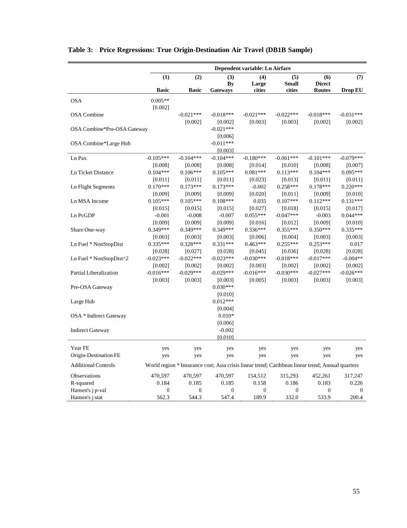
55

Table 3: Price Regressions: True Origin-Destination Air Travel (DB1B Sample)

Dependent variable: Ln Airfare

(1)

Basic

(2)

Basic

(3)

By

Gateways

(4)

Large

cities

(5)

Small

cities

(6)

Direct

Routes

(7)

Drop EU

OSA 0.005**

[0.002] OSA Combine -0.021*** -0.018*** -0.021*** -0.022*** -0.018*** -0.031***

[0.002] [0.002] [0.003] [0.003] [0.002] [0.002]

OSA Combine*Pre-OSA Gateway -0.021*** [0.006]

OSA Combine*Large Hub -0.011*** [0.003]

Ln Pax -0.105*** -0.104*** -0.104*** -0.180*** -0.061*** -0.101*** -0.079***

[0.008] [0.008] [0.008] [0.014] [0.010] [0.008] [0.007]

Ln Ticket Distance 0.104*** 0.106*** 0.105*** 0.081*** 0.113*** 0.104*** 0.095***

[0.011] [0.011] [0.011] [0.023] [0.013] [0.011] [0.011]

Ln Flight Segments 0.170*** 0.173*** 0.173*** -0.002 0.258*** 0.178*** 0.220***

[0.009] [0.009] [0.009] [0.020] [0.011] [0.009] [0.010]

Ln MSA Income 0.105*** 0.105*** 0.108*** 0.035 0.107*** 0.112*** 0.131***

[0.015] [0.015] [0.015] [0.027] [0.018] [0.015] [0.017]

Ln PcGDP -0.001 -0.008 -0.007 0.055*** -0.047*** -0.003 0.044***

[0.009] [0.009] [0.009] [0.016] [0.012] [0.009] [0.010]

Share One-way 0.349*** 0.349*** 0.349*** 0.336*** 0.355*** 0.350*** 0.335***

[0.003] [0.003] [0.003] [0.006] [0.004] [0.003] [0.003]

Ln Fuel * NonStopDist 0.335*** 0.328*** 0.331*** 0.463*** 0.255*** 0.253*** 0.017

[0.028] [0.027] [0.028] [0.045] [0.036] [0.028] [0.028]

Ln Fuel * NonStopDist^2 -0.023*** -0.022*** -0.023*** -0.030*** -0.018*** -0.017*** -0.004**

[0.002] [0.002] [0.002] [0.003] [0.002] [0.002] [0.002]

Partial Liberalization -0.016*** -0.029*** -0.029*** -0.016*** -0.030*** -0.027*** -0.026***

[0.003] [0.003] [0.003] [0.005] [0.003] [0.003] [0.003]

Pre-OSA Gateway 0.030*** [0.010]

Large Hub 0.012*** [0.004]

OSA * Indirect Gateway 0.010* [0.006]

Indirect Gateway -0.002 [0.010]

Year FE yes yes yes yes yes yes yes

Origin-Destination FE yes yes yes yes yes yes yes

Additional Controls World region * Insurance cost; Asia crisis linear trend; Caribbean linear trend; Annual quarters

Observations 470,597 470,597 470,597 154,512 315,293 452,261 317,247

R-squared 0.184 0.185 0.185 0.158 0.186 0.183 0.226

Hansen's j p-val 0 0 0 0 0 0 0

Hansen's j stat 562.3 544.3 547.4 189.9 332.0 533.9 200.4

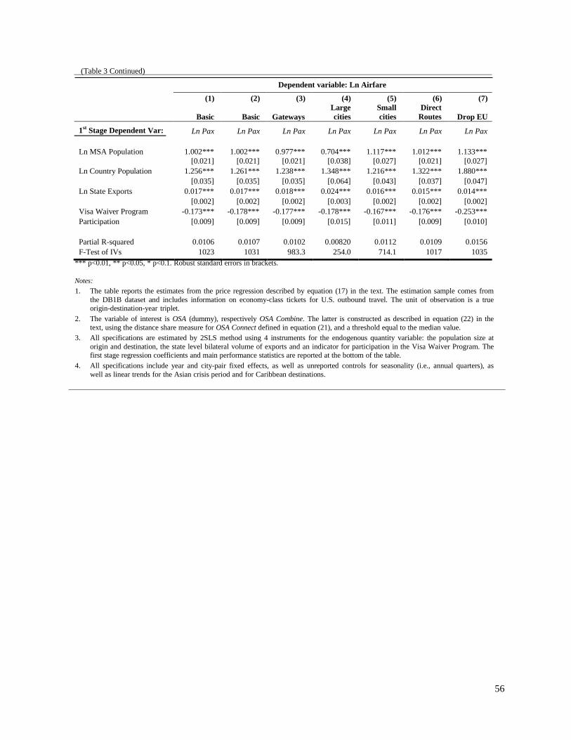
56

(Table 3 Continued)

Dependent variable: Ln Airfare

*** p<0.01, ** p<0.05, * p<0.1. Robust standard errors in brackets.

Notes:

1. The table reports the estimates from the price regression described by equation (17) in the text. The estimation sample comes from

the DB1B dataset and includes information on economy-class tickets for U.S. outbound travel. The unit of observation is a true

origin-destination-year triplet.

2. The variable of interest is OSA (dummy), respectively OSA Combine. The latter is constructed as described in equation (22) in the

text, using the distance share measure for OSA Connect defined in equation (21), and a threshold equal to the median value.

3. All specifications are estimated by 2SLS method using 4 instruments for the endogenous quantity variable: the population size at

origin and destination, the state level bilateral volume of exports and an indicator for participation in the Visa Waiver Program. The

first stage regression coefficients and main performance statistics are reported at the bottom of the table.

4. All specifications include year and city-pair fixed effects, as well as unreported controls for seasonality (i.e., annual quarters), as

well as linear trends for the Asian crisis period and for Caribbean destinations.

(1)

Basic

(2)

Basic

(3)

Gateways

(4)

Large

cities

(5)

Small

cities

(6)

Direct

Routes

(7)

Drop EU

1st

Stage Dependent Var: Ln Pax Ln Pax Ln Pax Ln Pax Ln Pax Ln Pax Ln Pax

Ln MSA Population

1.002***

1.002***

0.977***

0.704***

1.117***

1.012***

1.133***

[0.021] [0.021] [0.021] [0.038] [0.027] [0.021] [0.027]

Ln Country Population 1.256*** 1.261*** 1.238*** 1.348*** 1.216*** 1.322*** 1.880***

[0.035] [0.035] [0.035] [0.064] [0.043] [0.037] [0.047]

Ln State Exports 0.017*** 0.017*** 0.018*** 0.024*** 0.016*** 0.015*** 0.014***

[0.002] [0.002] [0.002] [0.003] [0.002] [0.002] [0.002]

Visa Waiver Program -0.173*** -0.178*** -0.177*** -0.178*** -0.167*** -0.176*** -0.253***

Participation [0.009] [0.009] [0.009] [0.015] [0.011] [0.009] [0.010]

Partial R-squared 0.0106 0.0107 0.0102 0.00820 0.0112 0.0109 0.0156

F-Test of IVs 1023 1031 983.3 254.0 714.1 1017 1035

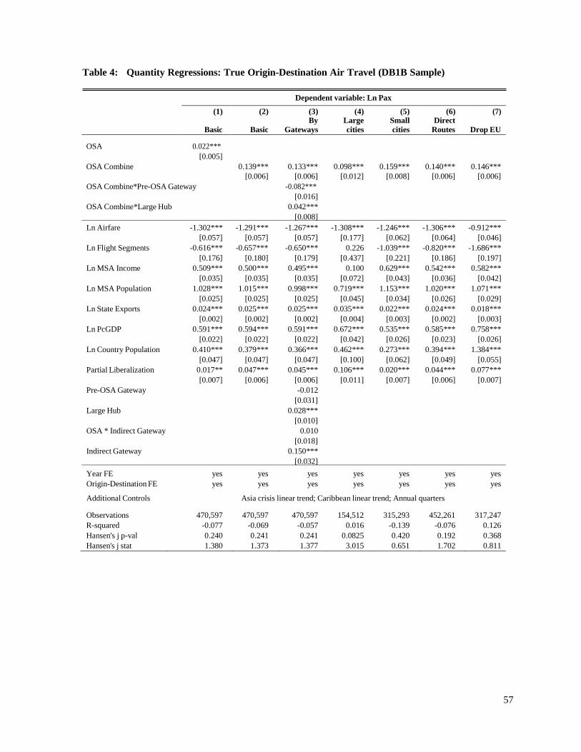
57

Table 4: Quantity Regressions: True Origin-Destination Air Travel (DB1B Sample)

Dependent variable: Ln Pax

(1) (2) (3) (4) (5) (6) (7)

By Large Small Direct Basic Basic Gateways cities cities Routes Drop EU

OSA

OSA Combine

0.022***

[0.005]

0.139***

0.133***

0.098***

0.159***

0.140***

0.146***

[0.006] [0.006] [0.012] [0.008] [0.006] [0.006]

OSA Combine*Pre-OSA Gateway -0.082***

[0.016]

OSA Combine*Large Hub 0.042***

[0.008]

Ln Airfare -1.302*** -1.291*** -1.267*** -1.308*** -1.246*** -1.306*** -0.912***

[0.057] [0.057] [0.057] [0.177] [0.062] [0.064] [0.046]

Ln Flight Segments -0.616*** -0.657*** -0.650*** 0.226 -1.039*** -0.820*** -1.686***

[0.176] [0.180] [0.179] [0.437] [0.221] [0.186] [0.197]

Ln MSA Income 0.509*** 0.500*** 0.495*** 0.100 0.629*** 0.542*** 0.582***

[0.035] [0.035] [0.035] [0.072] [0.043] [0.036] [0.042]

Ln MSA Population 1.028*** 1.015*** 0.998*** 0.719*** 1.153*** 1.020*** 1.071***

[0.025] [0.025] [0.025] [0.045] [0.034] [0.026] [0.029]

Ln State Exports 0.024*** 0.025*** 0.025*** 0.035*** 0.022*** 0.024*** 0.018***

[0.002] [0.002] [0.002] [0.004] [0.003] [0.002] [0.003]

Ln PcGDP 0.591*** 0.594*** 0.591*** 0.672*** 0.535*** 0.585*** 0.758***

[0.022] [0.022] [0.022] [0.042] [0.026] [0.023] [0.026]

Ln Country Population 0.410*** 0.379*** 0.366*** 0.462*** 0.273*** 0.394*** 1.384***

[0.047] [0.047] [0.047] [0.100] [0.062] [0.049] [0.055]

Partial Liberalization 0.017** 0.047*** 0.045*** 0.106*** 0.020*** 0.044*** 0.077***

[0.007] [0.006] [0.006] [0.011] [0.007] [0.006] [0.007]

Pre-OSA Gateway -0.012 [0.031]

Large Hub 0.028***

[0.010]

OSA * Indirect Gateway 0.010

[0.018]

Indirect Gateway 0.150***

[0.032]

Year FE yes yes yes yes yes yes yes

Origin-Destination FE yes yes yes yes yes yes yes

Additional Controls Asia crisis linear trend; Caribbean linear trend; Annual quarters

Observations 470,597 470,597 470,597 154,512 315,293 452,261 317,247

R-squared -0.077 -0.069 -0.057 0.016 -0.139 -0.076 0.126

Hansen's j p-val 0.240 0.241 0.241 0.0825 0.420 0.192 0.368

Hansen's j stat 1.380 1.373 1.377 3.015 0.651 1.702 0.811

58

(Table 4 Continued)

Dependent variable: Ln Pax

*** p<0.01, ** p<0.05, * p<0.1. Robust standard errors in brackets.

Notes:

1. The table reports the estimates from the quantity regression described by equation (18) in the text. The estimation sample comes

from the DB1B dataset and includes information on economy-class tickets for U.S. outbound travel. The unit of observation is a true

origin-destination-year triplet.

2. The variable of interest is OSA (dummy), respectively OSA Combine. The latter is constructed as described in equation (22) in the

text, using the passenger share measure for OSA Connect defined in equation (20), and a threshold value equal to the 25th percentile.

3. All specifications are estimated by 2SLS method. The excluded instruments for the endogenous price and flight segments variables

are: the non-stop distance between the origin and destination cities interacted with fuel prices, the excess travel distance in the base

year calculated relative to the non-stop distance, and its squared value, both interacted with fuel prices. The first stage regression

coefficients and main performance statistics are reported at the bottom of the table.

4. All specifications include year and city-pair fixed effects, as well as unreported controls for seasonality (i.e., annual quarters), as

well as linear trends for the Asian crisis period and for Caribbean destinations.

(1)

Basic

(2)

Basic

(3)

By

Gateways

(4)

Large

cities

(5)

Small

cities

(6)

Direct

Routes

(7)

Drop EU

1st

Stage Dependent Var: Ln Airfare Ln Airfare Ln Airfare Ln Airfare Ln Airfare Ln Airfare Ln Airfare

Ln Fuel * ExcessDistance

-0.032

-0.033

-0.316***

0.000

-0.062**

-0.025

-0.051**

Ln Fuel *

[0.023] [0.023] [0.022] [0.047] [0.026] [0.023] [0.023]

ExcessDistance^2 0.300*** 0.299*** 0.298*** 0.329*** 0.293*** 0.304*** 0.197***

[0.042] [0.042] [0.042] [0.081] [0.051] [0.042] [0.045]

Ln Fuel * NonStopDist -0.071*** -0.071*** -0.071*** -0.041*** -0.082*** -0.066*** -0.085***

[0.002] [0.002] [0.002] [0.003] [0.002] [0.002] [0.002]

Partial R-squared 0.00423 0.00430 0.00428 0.00210 0.00524 0.00382 0.00867

F-Test of IVs 668.7 679.5 676.7 108.1 537.3 577.3 849.2

1st

Stage Dependent Var: Ln Segm Ln Segm Ln Segm Ln Segm Ln Segm Ln Segm Ln Segm

Ln Fuel * ExcessDistance

0.021**

0.020**

-0.241***

0.037

0.013

0.016*

0.006

Ln Fuel *

[0.010] [0.010] [0.009] [0.023] [0.010] [0.010] [0.010]

ExcessDistance^2 0.277*** 0.275*** 0.275*** 0.250*** 0.279*** 0.274*** 0.244***

[0.017] [0.017] [0.017] [0.039] [0.019] [0.017] [0.019]

Ln Fuel * NonStopDist 0.000 -0.001 -0.001 0.003** -0.005*** -0.003*** -0.001

[0.001] [0.001] [0.001] [0.001] [0.001] [0.001] [0.001]

Partial R-squared 0.00354 0.00347 0.00346 0.00209 0.00379 0.00352 0.00345

F-Test of IVs 448.6 438.5 437.4 82.27 322.1 425.3 299.9

59

Table 5: Impact of Air Liberalization on the Number of U.S. Exit Points Used per Origin-

Destination Route (DB1B Sample)

Dependent variable: Ln Number US Exit Points

*** p<0.01, ** p<0.05, * p<0.1. Robust standard errors in brackets.

Notes:

1. The table reports the estimates from a regression specification similar to equation (19) in the text, except that the dependent variable in this

case is the number of distinct U.S. exit points transited by passengers from an origin city o going to the final destination d at time t. The sample and estimation specification descriptions from Tables 3 and 4 apply here as well.

2. The variable of interest is OSA Combine, which is constructed as described in equation (22) in the text, using the distance share measure for

OSA Connect defined in equation (21), and a threshold equal to the median value. All specifications are estimated by 2SLS method. The first stage regression coefficients and main performance statistics are reported at the bottom of the table.

(1) (2) (3)

OSA Combine

OSA Combine*Pre-OSA Gateway

OSA Combine*Large Hub

OSA Combine*Large Hub (T100)

0.027***

[0.002]

0.035***

[0.003]

-0.062***

[0.008]

-0.005

[0.005]

0.034***

[0.002]

-0.062***

[0.008]

-0.104***

[0.010]

Ln Pax

Ln MSA Income

Ln PcGDP

Share One-way

Partial Liberalization

Pre-OSA Gateway

Large Hub

OSA * Indirect Gateway

Indirect Gateway

0.483***

[0.022]

-0.028

[0.018]

-0.087***

[0.019]

-0.055***

[0.002]

-0.032***

[0.003]

0.481***

[0.022]

-0.018

[0.018]

-0.086***

[0.019]

-0.055***

[0.002]

-0.034***

[0.003]

-0.053***

[0.014]

-0.023***

[0.005]

-0.021***

[0.008]

-0.061***

[0.016]

0.484***

[0.022]

-0.021

[0.019]

-0.089***

[0.019]

-0.055***

[0.002]

-0.035***

[0.003]

-0.052***

[0.014]

--

-0.021***

[0.008]

-0.063***

[0.016]

Year FE

Origin-Destination FE

yes

yes

yes

yes

yes

yes

Observations 470,597 470,597 470,597

R-squared 0.275 0.276 0.275

Hansen's j p-val 0.142 0.371 0.427

Hansen's j stat 2.152 0.800 0.632

First Stage Dependent Var: Ln Pax Ln Pax Ln Pax

Ln State Exports

Visa Waiver Program Participation

0.030***

[0.002]

-0.185***

[0.009]

0.031***

[0.002]

-0.186***

[0.009]

0.030***

[0.002]

-0.185***

[0.009]

Partial R-squared 0.00167 0.00172 0.00167

F-Test of IVs 365.5 375.4 365.5

Table 6: Flight Segments Regressions: True Origin-Destination Air Travel (DB1B Sample)

Dependent variable: Ln Flight Segments

(1) (2) (3) (4) (5) (6) (7) (8)

OSA OSA

By

Gateways

By

Gateways

Large

cities

Small

cities

Direct

Routes Drop EU

OSA -0.004***

[0.001]

OSA Combine 0.012*** 0.009*** 0.012*** 0.006*** 0.014*** 0.012*** 0.006***

[0.001] [0.001] [0.001] [0.001] [0.001] [0.001] [0.001]

OSA Combine*Pre-OSA 0.003 -0.004

Gateway [0.003] [0.003]

OSA Combine*Large Hub 0.011***

[0.002]

OSA Combine*Large Hub (T100) -0.045***

[0.003]

Ln Pax -0.060*** -0.065*** -0.065*** -0.065*** -0.051*** -0.069*** -0.080*** -0.078***

[0.007] [0.007] [0.007] [0.007] [0.010] [0.010] [0.008] [0.006]

Ln MSA Income 0.038*** 0.040*** 0.039*** 0.041*** -0.030*** 0.065*** 0.049*** 0.079***

[0.006] [0.006] [0.006] [0.006] [0.011] [0.007] [0.006] [0.007]

Ln PcGDP -0.017*** -0.011* -0.011* -0.011* -0.025*** -0.010 -0.008 -0.008

[0.006] [0.006] [0.006] [0.006] [0.009] [0.008] [0.007] [0.007]

Share One-way 0.022*** 0.022*** 0.022*** 0.022*** 0.028*** 0.019*** 0.022*** 0.014***

[0.001] [0.001] [0.001] [0.001] [0.002] [0.001] [0.001] [0.001]

Partial Liberalization -0.011*** -0.004*** -0.004*** -0.004*** -0.000 -0.005*** -0.004*** -0.001

[0.001] [0.001] [0.001] [0.001] [0.002] [0.001] [0.001] [0.001]

Pre-OSA Gateway -0.088*** -0.085***

[0.005] [0.005]

Large Hub -0.012***

[0.002]

OSA * Indirect Gateway 0.005*

0.010*** [0.003]

[0.003]

Indirect Gateway -0.033*** -0.035***

[0.005] [0.005]

Year FE yes yes yes yes yes yes yes yes

Origin-Destination FE yes yes yes yes yes yes yes yes

Additional Controls Asia crisis linear trend; Caribbean linear trend; Annual quarters

Observations 470,597 470,597 470,597 470,597 154,512 315,293 452,261 317,247

R-squared 0.090 0.082 0.085 0.085 0.107 0.069 0.059 0.077

Hansen's j p-val 0.00235 0.00882 0.0129 0.00527 0.00419 0.375 4.29e-05 0.200

Hansen's j stat 9.252 6.858 6.187 7.784 8.199 0.787 16.74 1.641

1st Stage Dependent Var: Ln Pax Ln Pax Ln Pax Ln Pax Ln Pax Ln Pax Ln Pax Ln Pax

Ln State Exports 0.030*** 0.029*** 0.031*** 0.030*** 0.039*** 0.030*** 0.030*** 0.037***

[0.002] [0.002] [0.002] [0.002] [0.003] [0.002] [0.002] [0.002]

Visa Waiver Program -0.179*** -0.159*** -0.186*** -0.185*** -0.209*** -0.185*** -0.180*** -0.272***

Participation [0.009] [0.011] [0.009] [0.009] [0.015] [0.009] [0.009] [0.010]

Partial R-squared 0.00159 0.00167 0.00172 0.00167 0.00237 0.00138 0.00155 0.00300

F-Test of IVs 348.0 365.5 375.4 365.5 172.8 191.1 331.7 498.1

*** p<0.01, ** p<0.05, * p<0.1. Robust standard errors in brackets.

Notes: The table reports the estimates from regression described by equation (19) in the text, using the number of flight segments per origin-destination market as the dependent variable. The sample and estimation specification descriptions from Tables 3 and 4 apply here as well. The variable of interest is

OSA Combine, which is constructed as described in equation (22) in the text, using the distance share measure for OSA Connect defined in equation (21), and a threshold equal to the median value. All specifications are estimated by 2SLS method. The first stage regression coefficients and main performance

statistics are reported at the bottom of the table. 60

61

Table 7: Consumer Welfare Calculations

Consumer Welfare Effects of OSA

Pooled

Estimates

Pre-OSA

Gateway Large Hub

Large

Hub T100 Small City

Total Price Effects: -0.041 -0.050 -0.053 -0.069 -0.038

Of which: Direct Effect: -0.021 -0.039 -0.029 -0.029 -0.018

Indirect Effect via Quantity: -0.020 -0.012 -0.025 -0.031 -0.019

Indirect Effect via Connectivity: 0.000 0.001 0.001 -0.009 -0.001

Total Quantity (Demand)Effects: 0.192 0.112 0.241 0.299 0.183

Of which:

Direct Effect: 0.139 0.051 0.175 0.175 0.133

Indirect Effect via Prices: 0.053 0.064 0.069 0.089 0.049

Indirect Effect via Connectivity: 0.000 -0.003 -0.003 0.034 0.002

Piece Equivalent Quality Effect: -0.108 -0.037 -0.133 -0.162 -0.105

Total tariff equivalent of OSA:

-0.149

-0.087

-0.187

-0.231

-0.142

Average Price Effect at U.S. Level

City Pop. Shares as Weights -0.144

City Pax Shares as Weights -0.143

Notes: The calculations reported in this table reflect a comparative statics exercise and correspond to the partial and total effects

resulting from the signing of an Open Skies Agreement (i.e., change in OSA from 0 to 1). The Empirical Methodology Appendix

2B provides the analytical details behind the comparative statics calculation. The calculations are done using average sample

estimates (pooled city sample), as well as estimates specific to each type of origin city. Rows 1 and 5 (in italics) report the total

effect of a change in OSA on the average price and aggregate quantity of travel in an origin-destination market. Each of these

total effects can be decomposed into partial effects consisting of a direct effect of a change in OSA, an indirect effect operating

via a change in price or quantity, and an indirect effect operating via a change in directness (i.e., the average number of

segments). These partial effects, which sum up to the total effect, are reported in rows 2-4 for prices, respectively 6-8 for

quantities. The quantity effect net of price changes (i.e., rows 6 and 8) correspond to a broadly defined quality effect. To express

it in price equivalent terms (row 9), the quality effect is divided by the price elasticity of demand. The total tariff equivalent of

OSA corresponds to the aggregate price drop generated by the price and quality effects (row 1 + row 9). The last two rows of the

table represent the weighted average of the tariff equivalents for each city type, where the weights reflect the U.S. population

share or passenger share accounted by those city types.

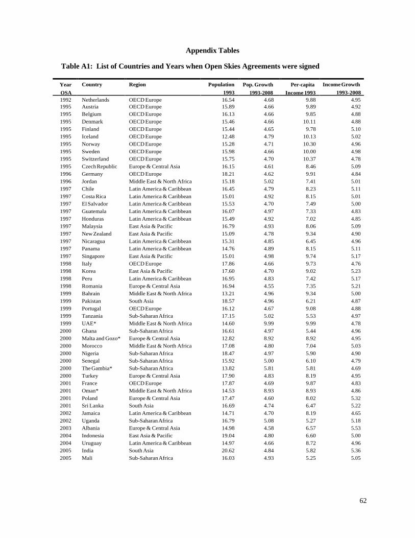
62

Appendix Tables

Table A1: List of Countries and Years when Open Skies Agreements were signed

Year

OSA

Country Region Population

1993

Pop. Growth

1993-2008

Per-capita

Income 1993

Income Growth

1993-2008

1992 Netherlands OECD Europe 16.54 4.68 9.88 4.95

1995 Austria OECD Europe 15.89 4.66 9.89 4.92

1995 Belgium OECD Europe 16.13 4.66 9.85 4.88

1995 Denmark OECD Europe 15.46 4.66 10.11 4.88

1995 Finland OECD Europe 15.44 4.65 9.78 5.10

1995 Iceland OECD Europe 12.48 4.79 10.13 5.02

1995 Norway OECD Europe 15.28 4.71 10.30 4.96

1995 Sweden OECD Europe 15.98 4.66 10.00 4.98

1995 Switzerland OECD Europe 15.75 4.70 10.37 4.78

1995 Czech Republic Europe & Central Asia 16.15 4.61 8.46 5.09

1996 Germany OECD Europe 18.21 4.62 9.91 4.84

1996 Jordan Middle East & North Africa 15.18 5.02 7.41 5.01

1997 Chile Latin America & Caribbean 16.45 4.79 8.23 5.11

1997 Costa Rica Latin America & Caribbean 15.01 4.92 8.15 5.01

1997 El Salvador Latin America & Caribbean 15.53 4.70 7.49 5.00

1997 Guatemala Latin America & Caribbean 16.07 4.97 7.33 4.83

1997 Honduras Latin America & Caribbean 15.49 4.92 7.02 4.85

1997 Malaysia East Asia & Pacific 16.79 4.93 8.06 5.09

1997 New Zealand East Asia & Pacific 15.09 4.78 9.34 4.90

1997 Nicaragua Latin America & Caribbean 15.31 4.85 6.45 4.96

1997 Panama Latin America & Caribbean 14.76 4.89 8.15 5.11

1997 Singapore East Asia & Pacific 15.01 4.98 9.74 5.17

1998 Italy OECD Europe 17.86 4.66 9.73 4.76

1998 Korea East Asia & Pacific 17.60 4.70 9.02 5.23

1998 Peru Latin America & Caribbean 16.95 4.83 7.42 5.17

1998 Romania Europe & Central Asia 16.94 4.55 7.35 5.21

1999 Bahrain Middle East & North Africa 13.21 4.96 9.34 5.00

1999 Pakistan South Asia 18.57 4.96 6.21 4.87

1999 Portugal OECD Europe 16.12 4.67 9.08 4.88

1999 Tanzania Sub-Saharan Africa 17.15 5.02 5.53 4.97

1999 UAE* Middle East & North Africa 14.60 9.99 9.99 4.78

2000 Ghana Sub-Saharan Africa 16.61 4.97 5.44 4.96

2000 Malta and Gozo* Europe & Central Asia 12.82 8.92 8.92 4.95

2000 Morocco Middle East & North Africa 17.08 4.80 7.04 5.03

2000 Nigeria Sub-Saharan Africa 18.47 4.97 5.90 4.90

2000 Senegal Sub-Saharan Africa 15.92 5.00 6.10 4.79

2000 The Gambia* Sub-Saharan Africa 13.82 5.81 5.81 4.69

2000 Turkey Europe & Central Asia 17.90 4.83 8.19 4.95

2001 France OECD Europe 17.87 4.69 9.87 4.83

2001 Oman* Middle East & North Africa 14.53 8.93 8.93 4.86

2001 Poland Europe & Central Asia 17.47 4.60 8.02 5.32

2001 Sri Lanka South Asia 16.69 4.74 6.47 5.22

2002 Jamaica Latin America & Caribbean 14.71 4.70 8.19 4.65

2002 Uganda Sub-Saharan Africa 16.79 5.08 5.27 5.18

2003 Albania Europe & Central Asia 14.98 4.58 6.57 5.53

2004 Indonesia East Asia & Pacific 19.04 4.80 6.60 5.00

2004 Uruguay Latin America & Caribbean 14.97 4.66 8.72 4.96

2005 India South Asia 20.62 4.84 5.82 5.36

2005 Mali Sub-Saharan Africa 16.03 4.93 5.25 5.05

63

* Growth rates are for the period 1993-2007.

Note: The following 16 countries have signed an Open Skies Agreement with the U.S. but there is missing data on either population or

income for the period of interest: Armenia (2008), Aruba (1997), Bosnia-Hercegovina (2007), Croatia (2008), Estonia (2007), Georgia

(2007), Kuwait (2006), Latvia (2006), Lithuania (2007), Luxembourg (1995), Quatar (2001), Slovakia (2000), Slovenia (2007), Tonga

(2003), Uzbekistan (1998), Western Samoa (2002).

2005 Paraguay Latin America & Caribbean 15.34 4.91 7.26 4.67

2005 Thailand East Asia & Pacific 17.89 4.74 7.45 5.04

2006 Cameroon Sub-Saharan Africa 16.41 4.97 6.39 4.77

2007 Bulgaria Europe & Central Asia 15.95 4.50 7.30 5.16

2007 Canada NAFTA 17.18 4.75 9.85 4.94

2007 Cyprus Europe & Central Asia 13.47 4.80 9.18 4.99

2007 Greece OECD Europe 16.16 4.67 9.18 5.05

2007 Hungary Europe & Central Asia 16.15 4.57 8.19 5.15

2007 Ireland OECD Europe 15.09 4.82 9.60 5.34

2007 Liberia Sub-Saharan Africa 14.48 5.27 4.42 5.18

2007 Spain OECD Europe 17.48 4.76 9.35 4.95

2007 United Kingdom OECD Europe 17.87 4.67 9.91 4.97

2008 Australia East Asia & Pacific 16.69 4.80 9.78 4.96

2008 Kenya Sub-Saharan Africa 17.07 5.01 6.02 4.70

2008 Laos East Asia & Pacific 15.33 4.91 5.49 5.27

64

Table A2: Testing for Endogeneity in the Timing of Open Skies Agreements

Dependent Variable: (Year OSA - 1992)

*** p<0.01, ** p<0.05, * p<0.1; Robust standard errors in brackets.

(1) (2) (3) (4) (5) (6)

Log Population 1993

Log Population Growth ‘93-‘08

Log GDP 1993

0.504

[0.307]

3.413

[3.422]

-0.154

0.180

[0.412]

-1.041

[4.363]

0.501

[0.513]

-7.399

[5.509]

Log GDP Growth ‘93-‘08

Log Per-Capita GDP 1993

[0.310]

3.635

[2.506]

-0.501

-0.470

-0.173

Log Per Capita GDP Growth ‘93-‘08

Log Exports 1993

[0.513]

3.292

[2.758]

-0.279

[0.692]

2.452

[3.561]

[1.062]

-2.564

[3.892]

Log Export Growth ‘93-‘08 [0.214]

-0.838

-0.420

-0.175

Log Distance

Log Average Tariffs (year 2001)

[0.688] [0.615]

1.499

[1.697]

[1.062]

0.683

High & Upper Middle Income Dummy

-1.299

-1.868

-1.568

[0.858]

-2.124

Constant

-16.101

-6.729

[1.611]

-3.277

[1.205]

19.862***

[1.661]

-8.113

[1.849]

51.420

[18.107] [17.785] [15.610] [6.570] [34.723] [47.141]

Observations 64 64 64 64 64 41

R-squared 0.039 0.048 0.124 0.105 0.160 0.171

65

Table A3: Summary Statistics

Variable Obs. Mean Std. Dev. Min. Max.

Policy Variables:

OSA 470606 0.386 0.487 0.000 1.000

OSA Combine (Dist) 470606 0.450 0.473 0.000 1.000

OSA Combine (Pax) 470606 0.531 0.499 0.000 1.000

Partial Liberalization 470606 0.215 0.411 0.000 1.000

Pre-OSA Gateway 470606 0.060 0.238 0.000 1.000

Large Hub 470606 0.266 0.442 0.000 1.000

Indirect Gateway 470606 0.054 0.225 0.000 1.000

Route Characteristics: Ln Pax (coach class) 470606 1.797 1.630 0.000 10.373

Ln Airfare 470606 1.623 0.544 -0.895 4.367

Ln Ticket Distance 470606 4820 2743 96 15998

(Pax) Share Direct Flight 470606 0.012 0.096 0.000 1.000

Ln Flight Segments 470606 0.961 0.221 0.000 1.386

(Pax) Share One-way 470606 0.148 0.249 0.000 1.000

Number US Exit Points 470606 2.933 2.650 1.000 36.000

Ln Number US Exit Points 470606 0.780 0.734 0.000 3.584

Ln Excess Distance (base year) 470606 0.120 0.114 -1.190 0.975

Demand and Cost Shifters: Ln MSA Population 470606 13.906 1.239 10.911 16.743

Ln MSA Income 470606 10.318 0.251 9.262 11.112

Ln Country Population 470606 17.126 1.803 10.600 21.001

Ln PcGDP 470606 8.960 1.267 4.817 11.189

Ln State Exports 470606 14.083 2.660 3.084 19.980

Insurance Cost Index 470606 162.544 76.414 79.288 320.907

Fuel Cost Index Visa Waiver Program

Participation

470606

470606

131.897

0.333

67.390

0.471

69.096

0.000

290.210

1.000

EU dummy 470606 0.326 0.469 0.000 1.000

NAFTA dummy 470606 0.215 0.411 0.000 1.000

Carribbean dummy 470606 0.182 0.386 0.000 1.000

Ln Fuel * ExcessDistance 470606 0.575 0.550 -5.554 5.530

Ln Fuel * ExcessDistance^2 470606 0.131 0.282 0.000 6.608

(Pax) Share Quarter 1 470606 0.219 0.267 0.000 1.000

(Pax) Share Quarter 2 470606 0.276 0.282 0.000 1.000

(Pax) Share Quarter 3 470606 0.262 0.281 0.000 1.000

(Pax) Share Quarter 4 470606 0.244 0.274 0.000 1.000

Note: The reported summary statistics correspond to the estimation sample used in generating the price, quantity and

directness effects reported in Tables 3-6.

66

!! !! ! ! !

! !! !! ! ! !

I. Theory Appendix

Appendix 1A:

In this appendix, we show that the final-stage local strategies given in Theorem 1 form a

final-stage local Nash equilibrium. The proof of uniqueness is contained in the Supplemental

Appendix. The following proof of existence focuses on the case that 𝑄! 𝑝 may be written as !

𝑄! 𝑝

=

! 𝑞!(𝑝) where 𝑞!(𝑝) is the non-negative Lebesgue-integrable derivative of 𝑄! 𝑝 . In

the Supplemental Appendix we examine an enlarged strategy space that allows for each 𝑄! 𝑝 to

contain a countable number35

of jump discontinuities (also known as mass points) and show that

there exists no equilibrium in which any player 𝑖’s cumulative price-quantity schedule 𝑄! 𝑝 contains a jump discontinuity.

In our proof that the final-stage local strategies given in Theorem 1 form a Nash equilibrium

in the final stage we focus on the case that there are 𝑚 ≥ 2 “active” normalized-cost types and show that for an alliance 𝑖 of an arbitrary normalized-cost type 𝑧 ≤ 𝑚 the equilibrium marginal price-quantity schedule 𝑞! 𝑝 is a best-response to 𝑞!! 𝑝 . The proof for the case of 𝑚 = 1 follows along similar lines.

The proof that the final-stage local strategies given in Theorem 1 form a Nash equilibrium has three steps. First, we formulate alliance 𝑖’s profit maximization problem as an optimal control problem and provide a necessary and sufficient condition for a global maximizer.

Second, we use Theorem 1 to construct 𝑞!!. Finally, we show that given 𝑞!! and alliance 𝑖’s necessary and sufficient condition for a global maximizer, alliance 𝑖’s unique best-response is the strategy 𝑞! specified by Theorem 1 for a type 𝑧 alliance. If alliance 𝑖 of normalized-cost type 𝑧 may feasibly provide direct service for a city pair, then alliance 𝑖’s final-stage local expected profit functional on that city pair is:

𝜋! 𝑞!, 𝑞∗ = 1 − 𝐹 𝑒 𝑝, 𝑞∗ + 𝑞 𝑝 − 𝜆 𝑞 𝑝 𝑑𝑝

(a1)

Similarly, if alliance 𝑖 is of the lowest normalized-cost type but may only feasibly provide

indirect service, then alliance 𝑖’s final-stage local expected profit functional on that route is:

𝜋! 𝑞!, 𝑞∗

= 𝛼 !

! 1 − 𝐹 𝑒 𝑝, 𝑞∗ + 𝑞 𝑝 − 𝜆 𝑞 𝑝 𝑑𝑝

(a2)

35 Note that as each 𝑄𝑖(𝑝) is a function of bounded variation it has, almost everywhere, a non-negative Lebesgue-

integrable derivative 𝑞𝑖 𝑝 and at most a countable number of jump discontinuities.

!

!

67

𝜂 𝑝

𝐷 𝑝

where the 𝛼 term on the right-hand side of (a2) arsises due to the fact that service is indirect. Because (a1) is equal to (a2) multiplied by a constant, we will, without loss of generality, refer to

(a1) as the profit functional of the lowest normalized-cost type alliance regradless of whether the

alliance offers direct or indirect service. We now formulate alliance 𝑖’s profit maximization problem as an optimal control problem. Let 𝑄!(𝑝) = 𝑞! 𝑝 ≡ 𝑢(𝑝) be the control. There is a monotonicity constraint on the control

variable, 𝑢 𝑝 ≥ 0. Recall that under proportional rationing 𝑒(𝑝, 𝑞) =

! !(!) 𝑑𝑟, let 𝑒 𝑝, 𝑞 ≡

! !(!)

𝑥(𝑝) be a state variable, and note that 𝑥 𝑝 = !!! ! !!(!)

. The boundary condition for the state

!(!)

variable is 𝑥 = 0. Let 𝜂(𝑝) denote the adjoint variable for the state variable. The

Hamiltonian for alliance 𝑖’s problem is

𝐻(𝑢(𝑝), 𝑥(𝑝), 𝜂(𝑝), 𝑝) = [(1 − 𝐹 (𝑥(𝑝)))𝑝 − 𝜆!]𝑢(𝑝) + 𝜂(𝑝)𝑥(𝑝)

Because the Hamiltonian is concave with respect to (𝑢, 𝑥), the (Pontryagin) Maximum

Principle provides the following necessary and sufficient conditions for a global maximizer:

𝜕𝐻

(a3)

= 1 − 𝐹 𝑥 𝑝 𝑝 − 𝜆! + = 0 𝜕𝐻

𝜂 𝑝 = − 𝜕𝑥 𝑝

= 𝐹′(𝑥(𝑝))𝑝𝑢(𝑝)

(a4)

Note that (a3), over the prices at which 𝑢(𝑝) > 0, may be written as

𝜂(𝑝) = −[(1 − 𝐹 (𝑥(𝑝)))𝑝 − 𝜆!]𝐷(𝑝) which implies that

𝜂(𝑝) = −(1 − 𝐹(𝑥(𝑝)))𝐷(𝑝) + 𝐹′(𝑥(𝑝)))𝑝𝑥(𝑝)𝐷(𝑝) − [(1 − 𝐹(𝑥(𝑝)))𝑝 − 𝜆!]𝐷′(𝑝)

which, when combined with (a4), provides the following necessary and sufficient optimality condition:

𝐹! 𝑥 𝑝 𝑝𝑞!! 𝑝 − 1 − 𝐹 𝑥 𝑝 𝐷 𝑝 − 1 − 𝐹 𝑥 𝑝 𝑝 − 𝜆! 𝐷!(𝑝) = 0. (a5)

which may be written as

𝑞!! 𝑝 = !! ! ! !

(a6)

where alliance 𝑖’s choice of price-quantity schedule, 𝑞! 𝑝 ≡ 𝑢(𝑝), enters into the right-hand

side of (a6) via the state variable 𝑥 𝑝 .

𝑝

𝜕𝑢 𝑝

!!! ! ! ! ! ! !!! ! ! !!!! !!(!)

68

!! ! !

! !!

!! ! !

!!! !!

!!∗(!)

!!(!!!(!!!∗(!)))

! ! !!! !![! ! !!"!(!)]

!"(!)( !!! !!!!)

!

Next, recall that Theorem 1 states that an equilibrium is given by

𝑞! 𝑝|𝑛!, 𝑛! = − 𝑛 𝜆 − 𝜆 𝑖𝑓 𝑝 ∈ [𝑝, 𝑝 )

!!! !!! !!!∗ !

⋮ ! ! ! ! !!!

− !!! !!! !!!∗ !

⋮ !!! 𝑛! 𝜆! − 𝜆! 𝑖𝑓 𝑝 ∈ [𝑝! , 𝑝!!!)

!(!)

!! 𝑖𝑓 𝑝 ∈ [𝑝!, 𝑝]

and for each “active” normalized cost-type 𝑗 = 2, … , 𝑚, an equilibrium price-quantity schedule

is, for 𝑝 ∈ [𝑝, 𝑝!!!]

𝑞! 𝑝|𝑛!, 𝑛! = 𝑞! 𝑝|𝑛!, 𝑛! +

and 𝑞! 𝑝|𝑛!, 𝑛! = 0 for 𝑝 > 𝑝!!!.

!! !

!!! !!! !!!∗ ! 𝜆! − 𝜆!

Thus, if all alliances other than 𝑖 are following their Theorem 1 strategy, then over each price

interval [𝑝!, 𝑝!!!) with 𝑘 ≥ 𝑧 it follows that for an alliance 𝑖 of type 𝑧,

𝑞!! 𝑝 = !!! !!!!

(a7)

! ! ( !!! !! !!)

!! !

− !!! !! 𝑛 𝜆 − 𝜆 +

!!! !! !!! !!! !!!∗ ! !!! ! ! !

!! !

!!! !!! !!!∗ ! !!! 𝑛! 𝜆! − 𝜆!

− ! !

!!! !!! !!!∗ ! 𝜆! − 𝜆!

Next, note that for the price interval [𝑝!, 𝑝!!!) !

!!! !!

𝑦∗ 𝑝|𝑛!, 𝑛! =

!!

!!!!

!!!! ! !!!!

!" ! !!! !!!! −

is the unique solution to the differential equation

𝑦 𝑝 + =

with boundary condition 𝑦∗ 𝑝!!!|𝑛!, 𝑛! =

!! .

!!!!

Thus, for all 𝑝 ∈ [𝑝, 𝑝!!!] (a7) may be written as

𝑞!! 𝑝 =

(a8)

!(!)

! !!

!(!)

!!! !!

!!∗(!)

!!(!!!(!!!∗(!)))

!!∗(!)

!!(!!!(!!!∗(!)))

!!∗ !

!! !!! !!!∗ !

!!! !!!!

!!! !!!!

!!!! ! !

! ! !" ! !!! !!!! !"

!

!" !

!!! !

!!! !!!!

!!! !!!! !!(!)

!"(!)( !!! !!!!)

!∗ ! ! ! ! !∗ ! !!!! !!(!)

!! !!! !!!∗ ! !

69

!∗ ! ! ! ! !∗ ! !!!! !!(!)

!! !!! !!!∗ ! !

!!!!

To summarize, (a8) provides the value of 𝑞!! 𝑝 if all alliances other than alliance 𝑖 follow

their Theorem 1 price-quantity schedules, and (a6) provides a necessary and sufficient condition

for a 𝑞!(𝑝) to be a best-response for alliance 𝑖. Setting (a6) equal to (a8), we have for each

𝑝 ∈ [𝑝, 𝑝!!!]

!! ! ! ! =

which holds with equality if and only if 1 − 𝐹 𝑥 𝑝 = 𝑦∗ 𝑝 for each 𝑝 ∈ [𝑝, 𝑝!!!], i.e., ! !!! ! !!!(!)

𝑑𝑟 = 𝐹!! 1 − 𝑦∗ 𝑝 for each 𝑝 ∈ [𝑝, 𝑝 ]. Thus, alliance 𝑖’s unique best-

! !(!) !!!

response is 𝑞! 𝑝|𝑛!, 𝑛! the Theorem 1 price-quantity schedule for a type 𝑧 alliance. To complete the proof, we now show that alliance 𝑖 of type 𝑧 has no incentive do deviate

from the price support of their equilibrium price quantity shcedule, [𝑝, 𝑝!!!]. Note that no alliance has incentive to offer tickets at prices strictly below 𝑝, because, by definition, tickets

priced at 𝑝 sell with probability 𝑦∗ = 1. Similarly, from Theorem 1, we know that tickets

priced at 𝑝!!! sell with probability 𝑦∗ 𝑝!!! = !! . Because 𝑦∗(⋅) is decreasing in price, no

type 𝑧 alliance offers tickets at prices strictly above 𝑝!!!. This completes the proof.

Appendix 1B:

This appendix provides the proofs for Propositions 1 and 2: (1) entry of a lowest normalized-

cost type alliance and any normalized cost decreasing compositional shift increase consumer

surplus, market capacity, and the average quantity and decrease the average (effective) price and (2) under Assumption 1, a similar result holds for the entry of any normalized-cost type alliance.

We focus on the case that the post-compositional shift satisfies 𝑛! < 𝑛 for each “active” normalized cost type alliance 𝑗. The remaining cases follow directly.

Beginning with the average ticket prices, which are calculated as ! 𝐷!! !(!(!,!)) !

! ! 𝐹 𝑒 𝑑𝑒

where 𝜌(𝑒, 𝑞) is the market-clearing price, or the highest price that a ticket is purchased given

the demand shock 𝑒 and the market price-quantity schedule 𝑞, which is given implicitly by 𝑒 𝜌 𝑒, 𝑞 , 𝑞 = 𝑒, and 𝑄 𝜌 𝑒, 𝑞 denotes the total quantity of tickets that are sold as a function of 𝜌 𝑒, 𝑞 and is calculated as

𝑝

!!! ! ! ! ! ! !!! ! ! !!!! !!(!)

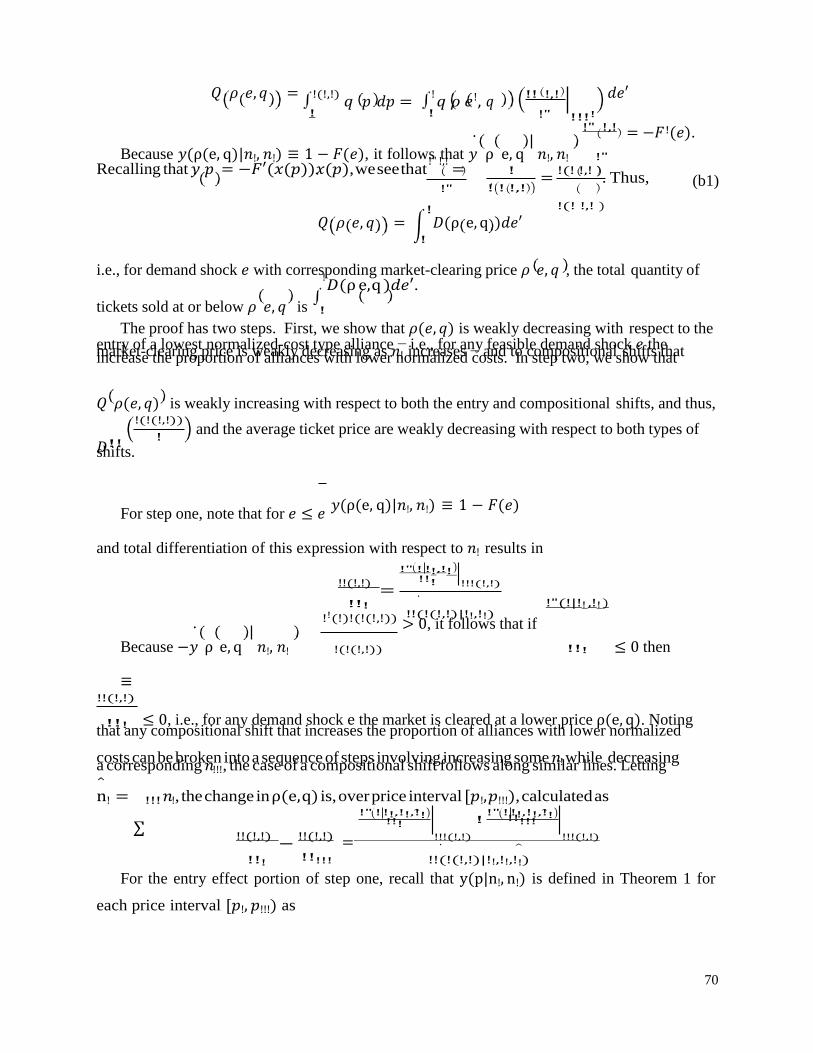
70

!

! ! !,!

!(!(!,!))

!

𝑄 𝜌 𝑒, 𝑞 = !(!,!) 𝑞 𝑝 𝑑𝑝 =

! 𝑞 𝜌 𝑒!, 𝑞

!! !,! 𝑑𝑒′ ! ! !" !!!!

!" !,! !

Because 𝑦(ρ(e, q)|𝑛!, 𝑛!) ≡ 1 − 𝐹(𝑒), it follows that 𝑦 ρ e, q 𝑛!, 𝑛!

= −𝐹 (𝑒).

!"

Recalling that 𝑦 𝑝 = −𝐹′(𝑥(𝑝))𝑥(𝑝), we see that !" !,!

= !"

!

= !(! !,! )

. Thus,

!(! !,! )

(b1)

𝑄 𝜌 𝑒, 𝑞 = 𝐷(ρ e, q )𝑑𝑒′ !

i.e., for demand shock 𝑒 with corresponding market-clearing price 𝜌 𝑒, 𝑞 , the total quantity of

tickets sold at or below 𝜌 𝑒, 𝑞 is

! 𝐷(ρ e, q )𝑑𝑒′.

!

The proof has two steps. First, we show that 𝜌(𝑒, 𝑞) is weakly decreasing with respect to the entry of a lowest normalized-cost type alliance − i.e., for any feasible demand shock 𝑒 the market-clearing price is weakly decreasing as 𝑛! increases − and to compositional shifts that increase the proportion of alliances with lower normalized costs. In step two, we show that

𝑄 𝜌(𝑒, 𝑞) is weakly increasing with respect to both the entry and compositional shifts, and thus,

𝐷!! and the average ticket price are weakly decreasing with respect to both types of

shifts.

For step one, note that for 𝑒 ≤ 𝑒

𝑦(ρ(e, q)|𝑛!, 𝑛!) ≡ 1 − 𝐹(𝑒)

and total differentiation of this expression with respect to 𝑛! results in

!" ! !!,!!

!!(!,!) =

!!!

!!(!)!(!(!,!))

!!! !!!(!,!)

!!(!(!,!)|!!,!!)

!"(!|!! ,!! )

Because −𝑦 ρ e, q 𝑛!, 𝑛!

≡

> 0, it follows that if

!(!(!,!)) !!! ≤ 0 then

!!(!,!)

!!! ≤ 0, i.e., for any demand shock e the market is cleared at a lower price ρ(e, q). Noting that any compositional shift that increases the proportion of alliances with lower normalized

costs can be broken into a sequence of steps involving increasing some 𝑛! while decreasing a corresponding 𝑛!!!, the case of a compositional shift follows along similar lines. Letting

n! = !!! 𝑛! , the change in ρ(e, q) is, over price interval [𝑝!, 𝑝!!!), calculated as !" ! !!,!!,!!

!!! !" ! !!,!!,!!

!!!!!

!!(!,!) −

!!(!,!) = !!!(!,!) !!!(!,!)

!!! !!!!! !!(!(!,!)|!!,!!,!!)

For the entry effect portion of step one, recall that y(p|n!, n!) is defined in Theorem 1 for

each price interval [𝑝!, 𝑝!!!) as

!

71

!!!! !

!

!!! !!!! !

!!!!

!!!! ! ! ! !" ! ! !! ! !"

!!

𝑦∗ 𝑝|𝑛!, 𝑛! =

!!

!!!!

!!!! ! !!!!

!" !

! !!! !!

!!! !!!! −

Then for each 𝑘 ∈ {2, … , 𝑚} , over [𝑝!, 𝑝!!!) !"(!|!! ,!! )

=

!!!

!!

!!!!

!!!! ! !!!!

!" !

!!! !!

!!! !!!! ln !!!! ! !!!!

!" !

!! !

!!! !!!!

!! !!! !! !!! !!! !!!! !!!! ! !! ! !" !

!

!!! !!!!!" !

!!! !!!! !" !

!!! !! +

!!! !!!!

! !!! !!!!

!

!!!!

! !! ! !" !

!

!!! !!!!

(!" !" ! !!"(!"(!)))!"

!!! !! ≤ 0

!!! !!!! !" ! !!! !!!!

A similar calculation shows that !"(!|!!,!!)

≤ 0 for 𝑝 ∈ [𝑝 , 𝑝]. Note that as 𝑝 is defined by

!!! !

!!

𝑦 𝑝 𝑛!, 𝑛! = 1 it follows

that

!!! < 0. Similarly, as 𝑝!!! is defined by 𝑝!!!𝑦 𝑝!!! 𝑛!, 𝑛! =

𝜆! it follows that !!!!! !! < 0. Note also that

!!!(!|!!,!!) !! !! ≤ 0,

!!!(!|!!,!!) ≤ 0, and

!! !" !!!(!|!!,!!)

≤

! ! ! !

0. We now examine the compositional shift portion of step one. Consider a portion of this shift

that involves an increase in 𝑛! with a decrease 𝑛!!!. For 𝑝 ∈ 𝑝!, 𝑝 , it follows from the

arguments above that !"(!|!!,!!,!!)

≤ 0, !"(!|!!,!!,!!)

= 0, and !!! < 0. For 𝑝 ∈ [𝑝, 𝑝 ), recall

!!! !!!!! !!! !!!

that n! = !!! 𝑛! and y(p|n!, n!, n!) is given by

𝑦∗ 𝑝|𝑛!, 𝑛!, n! =

!!

!!!!

!!

!!!! ! !!!! !!!! −

!" !

!" !

!

!!!!

The effect of the compositional shift is calculated as

!"(!|!! ,!! ,!! ) −

!" ! !! ,!! ,!! =

𝜆

− 𝜆 !!!! !

− ! ! ! !" !

! !!!!!"

≤ 0

!!! !!!!! ! !!! !!!! !" !

!!

!!!!

!!! !!!!

!!! !!!!

!!!!

! ! ! ! !" ! !!! !!!! !"

!

!" !

!!! !

!!! !!!!

+

!

72

which as before implies a decrease in the lower bound of the price support 𝑝. To summarize, we have shown that both the entry and compositional shifts result in a decrease in the equilibrium

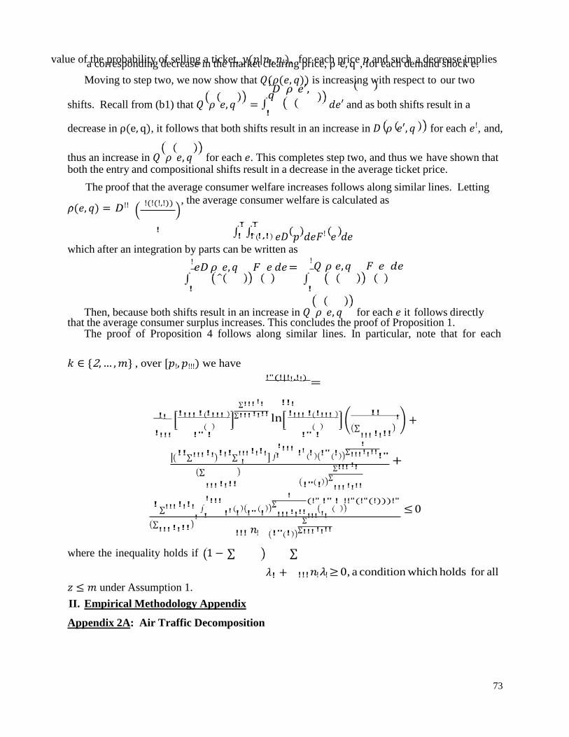
73

value of the probability of selling a ticket, 𝑦(𝑝|𝑛!, 𝑛!), for each price 𝑝 and such a decrease implies a corresponding decrease in the market clearing price, ρ e, q , for each demand shock e.

Moving to step two, we now show that 𝑄(𝜌(𝑒, 𝑞)) is increasing with respect to our two

shifts. Recall from (b1) that 𝑄 𝜌 𝑒, 𝑞 =

! 𝐷 𝜌 𝑒′,

𝑞

! 𝑑𝑒′ and as both shifts result in a

decrease in ρ(e, q), it follows that both shifts result in an increase in 𝐷 𝜌 𝑒′, 𝑞 for each 𝑒!, and,

thus an increase in 𝑄 𝜌 𝑒, 𝑞 for each 𝑒. This completes step two, and thus we have shown that both the entry and compositional shifts result in a decrease in the average ticket price.

The proof that the average consumer welfare increases follows along similar lines. Letting

𝜌(𝑒, 𝑞) = 𝐷!! !(!(!,!))

!

, the average consumer welfare is calculated as

𝑒𝐷 𝑝 𝑑𝑒𝐹! 𝑒 𝑑𝑒 which after an integration by parts can be written as

! 𝑒𝐷 𝜌 𝑒, 𝑞 𝐹 𝑒 𝑑𝑒 =

!

! 𝑄 𝜌 𝑒, 𝑞 𝐹 𝑒 𝑑𝑒

!

Then, because both shifts result in an increase in 𝑄 𝜌 𝑒, 𝑞 for each 𝑒 it follows directly that the average consumer surplus increases. This concludes the proof of Proposition 1.

The proof of Proposition 4 follows along similar lines. In particular, note that for each

𝑘 ∈ {2, … , 𝑚} , over [𝑝!, 𝑝!!!) we have

!!! !!

!"(!|!! ,!! ) =

!!!

!!

!!!!

!!!! ! !!!!

!" !

!!! !!!! ln !!!! ! !!!!

!" !

!! !

!!! !!!!

!! !!! !! !!! !!! !!!! !!!! ! !! ! !" !

!

!!! !!!!!" !

!!! !!!! !" !

!!! !! +

!!! !!!!

! !!! !!!!

!

!!!!

! !! ! !" !

!

!!! !!!!

(!" !" ! !!"(!"(!)))!"

!!! !! ≤ 0

!!! !!!!

where the inequality holds if 1 −

𝑧 ≤ 𝑚 under Assumption 1.

!!! 𝑛! !" !

𝜆! +

!!! !!!!

!!! 𝑛! 𝜆! ≥ 0, a condition which holds for all

II. Empirical Methodology Appendix

Appendix 2A: Air Traffic Decomposition

! !

! ! !,!

+

74

To motivate our analysis, we examine traffic growth patterns using the T-100 International

segment data. Total air passenger traffic between the United States and destination country d at

time t is defined as the sum of traffic across all routes r and carriers c.

𝑄!" = ! 𝑄!∈!"

=

! ! 𝑄!,!∈!"

We are interested in aggregate traffic growth with country d, as well as a decomposition of

that growth into new routes and old routes. For this decomposition, we treat each city-pair route

within country d as a distinct traded ‘variety’, but aggregate over carriers. That is, we count

Chicago-Paris as distinct from Atlanta-Paris, but do not distinguish whether that service was

operated by United Airlines or Air France. 36

One simple decomposition of Qdt is to count the number of routes offered Ndt and the

average passenger volume per route at a given point in time:

𝑄!" = 𝑄!"# = 𝑁!" ∗ 𝑄!"

!

A drawback of this approach is that it treats all air services as having equal value weights in

the total consumption of international travel. Alternatively, we can assess the importance of each

aviation route using its share of passenger shares for country d. Similar to the extensive margin

calculation in Feenstra (1994) and the decomposition method in Hummels and Klenow (2005),

we denote by Idt the set of all routes offered between the US and country d in period t, and by Id

the subset of routes operated between the US and country d in both the reference period t0 and 37

current period t, i.e., 𝐼! ⊆ 𝐼!" ⋂𝐼!"! .

decomposed as follows:

Then the total bilateral volume of air passengers can be

𝑄!" = !∈!! 𝑄!"# 𝜆!"

!! where 𝜆!" =

36 Retaining carrier specific traffic information is difficult as carriers frequently enter/exit particular routes, change

names, merge, and go out of business. In instances where it is possible to track longer time series for multiple

carriers on the same route, we can estimate elasticities of substitution between carriers. We find elasticities of

substitution between carriers on a given route almost an order of magnitude larger than elasticities across routes.

!∈!! !!"#

!∈!!" !!"#

75

37 In the empirical exercises, we will define the common variety set Ij to include those varieties that are have been

available in the current year as well as there years before. This ensures that experimental or temporary aviation

routes are excluded from Ij. We also experiment with a common variety set including routes offered both currently

and in the previous year.

76

d,93

The first term of the decomposition -- the intensive margin -- measures the volume of air

traffic accounted by aviation routes that are available in both the current and reference periods.

The lambda term represents the (passenger-share) weighted count of aviation routes to country d

available in both time periods. Alternatively, the lambda term can be viewed as one minus the

passenger-share weighted count of aviation routes that are “new” relative to the reference

period.38

It is useful to express total air traffic in terms of annual growth rates as follows:

!!" =

!!"!!

!!" !!

!!"!!

In this formulation, the first bracketed term captures the growth in air passenger traffic on

“common” service varieties (routes), while the second bracketed term measures the net change in

route offerings between two consecutive years. A lambda-ratio greater (less) than one implies a

gain (loss) in service varieties. The benefit of expressing the extensive margin as a net measure is

that in this way it accounts not only for new route additions, but also for any disappearing routes

since the reference period. However, if adding or withdrawing city-pair routes are discrete, less

frequent events, then cumulative (rather than annual) growth rates are a better way to decompose

growth. Summing the annual growth rates over time periods until the current year, we get an

expression for the cumulative air traffic growth relative to the first sample year 1993:

!" !" !" !" !" !!"

∆𝑄!" = ∆𝐼𝑀!" ∗

∆𝐸𝑀!"

where ∆𝑍!" = !!!""# ! !"!!

and Z {Q, IM, EM}, with each element defined as in equation (9). We normalize Z93

to

one.

Appendix 2B: Consumer Welfare Calculation

38 If all routes carried the same traffic volume (i.e., they have equal weights), then the lambda term would

!∈!! !!"#

!∈!! !!"#!!

77

correspond to the fraction of routes from the total number currently offered, that were already available in the

reference period. If traffic on new routes is non-negligible, then the inverse of lambda - the extensive margin - is

large, having an important contribution towards the total bilateral air traffic flow.

78

𝜕𝑙𝑛𝑃 𝜕𝑂𝑆𝐴

𝜕𝑙𝑛𝑄 𝜕𝑂𝑆𝐴

𝜕𝑙𝑛𝑆𝑒𝑔

𝜕𝑂𝑆𝐴

𝐽!

𝐽

Estimated regressions:

𝑙𝑛𝑃 = 𝛽!𝑙𝑛𝑄 + 𝛽!𝑙𝑛𝑆𝑒𝑔 +𝛽!𝑂𝑆𝐴 + 𝛽!𝑙𝑛𝑍 𝑙𝑛𝑄 = 𝛾!𝑙𝑛𝑃 + 𝛾!𝑙𝑛𝑆𝑒𝑔 + 𝛾!𝑂𝑆𝐴 + 𝛾!𝑙𝑛𝑍

𝑙𝑛𝑆𝑒𝑔 = 𝛿!𝑙𝑛𝑄 + 𝛿!𝑂𝑆𝐴 + 𝛿!𝑙𝑛𝑍

where Z is a vector of variables that is independent of the OSA aviation policy. The resulting system of simultaneous equation can be written as:

𝐹! 𝑙𝑛𝑃, 𝑙𝑛𝑄, 𝑙𝑛𝑆𝑒𝑔; 𝑂𝑆𝐴 = −𝑙𝑛𝑃 + 𝛽!𝑙𝑛𝑄 + 𝛽!𝑙𝑛𝑆𝑒𝑔 + 𝛽!𝑂𝑆𝐴 + 𝛽!𝑙𝑛𝑍 = 0

𝐹! 𝑙𝑛𝑃, 𝑙𝑛𝑄, 𝑙𝑛𝑆𝑒𝑔; 𝑂𝑆𝐴 = 𝛾!𝑙𝑛𝑃 − 𝑙𝑛𝑄 + 𝛾!𝑙𝑛𝑆𝑒𝑔 + 𝛾!𝑂𝑆𝐴 + 𝛾!𝑙𝑛𝑍 = 0

𝐹! 𝑙𝑛𝑃, 𝑙𝑛𝑄, 𝑙𝑛𝑆𝑒𝑔; 𝑂𝑆𝐴 = 𝛿!𝑙𝑛𝑄 − 𝑙𝑛𝑆𝑒𝑔 + 𝛿!𝑂𝑆𝐴 + 𝛿!𝑙𝑛𝑍 = 0

Taking the partial derivatives with respect to the policy variable OSA leads to the following:

𝜕𝑙𝑛𝑃 𝜕𝑙𝑛𝑄 𝜕𝑙𝑛𝑆𝑒𝑔 −

𝜕𝑂𝑆𝐴 + 𝛽! 𝜕𝑂𝑆𝐴

+ 𝛽! 𝜕𝑂𝑆𝐴

= −𝛽!

𝜕𝑙𝑛𝑃

𝛾! 𝜕𝑂𝑆𝐴

−

𝜕𝑙𝑛𝑄 + 𝛾!

𝜕𝑂𝑆𝐴 𝜕𝑙𝑛𝑄

𝛿! 𝜕𝑂𝑆𝐴 −

𝜕𝑙𝑛𝑆𝑒𝑔 = − 𝛾!

𝜕𝑂𝑆𝐴 𝜕𝑙𝑛𝑆𝑒𝑔

𝜕𝑂𝑆𝐴 = −𝛿!

This can be written in matrix form as:

−1 𝛽! 𝛽!

𝛾! −1 𝛾!

0 𝛿!

−1

−𝛽!

= −𝛾!

−𝛿!

with the relevant Jacobian determinant equal to:

−1 𝛽! 𝛽!

𝐽 =

𝛾! −1 𝛾!

0 𝛿!

−1

= −1 + 𝛽!𝛾!𝛿! + 𝛽!𝛾! + 𝛿!𝛾!

By Cramer’s rule, the solution comparative statics derivatives are given by:

𝜕𝑙𝑛𝑃

𝜕𝑂𝑆𝐴 = =

− 𝛽! 𝛾! + 𝛾!𝛿! − 𝛽! 𝛾!𝛿! + 𝛿! + 𝛽! (−1 + 𝛿!𝛾!)

−1 + 𝛽!𝛾!𝛿! + 𝛽!𝛾! + 𝛿!𝛾!

79

𝜕𝑙𝑛𝑄 −𝛾! − 𝛽!𝛾!𝛿! − 𝛾!𝛽! − 𝛿!𝛾!

𝜕𝑂𝑆𝐴 =

=

−1 + 𝛽 𝛾 𝛿 + 𝛽 𝛾 + 𝛿 𝛾

! ! ! ! ! ! !

𝜕𝑙𝑛𝑆𝑒𝑔 −𝛿! − 𝛾!𝛿!𝛽! + 𝛽!𝛾!𝛿! − 𝛿!𝛾!

𝜕𝑂𝑆𝐴 =

=

−1 + 𝛽 𝛾 𝛿 + 𝛽 𝛾 + 𝛿 𝛾

! ! ! ! ! ! !

𝐽!

𝐽

𝐽!

𝐽

80

Once the total derivatives are calculated, we can use the equations in (2) to decompose the

effect of the policy change on each variable of interest into direct and indirect effects (via the

other endogenous variables), as follows:

𝜕𝑙𝑛𝑃 𝜕𝑙𝑛𝑄 𝜕𝑙𝑛𝑆𝑒𝑔

𝜕𝑂𝑆𝐴 = 𝛽! + 𝛽! 𝜕𝑂𝑆𝐴

+

𝛽!

𝜕𝑂𝑆𝐴

𝜕𝑙𝑛𝑄 𝜕𝑙𝑛𝑃 𝜕𝑙𝑛𝑆𝑒𝑔

𝜕𝑂𝑆𝐴 = 𝛾! + 𝛾! 𝜕𝑂𝑆𝐴

+

𝛾!

𝜕𝑂𝑆𝐴

To calculate the price equivalent of air liberalization, we first convert the indirect effects of

OSA on air traffic (Q) into price equivalents, and then add them to the total price effect:

𝑃𝑟𝑖𝑐𝑒 𝑒𝑞𝑢𝑖𝑣𝑎𝑙𝑒𝑛𝑡 𝑜𝑓 𝑂𝑆𝐴

=

𝛾! + 𝛾!

𝜕𝑙𝑛𝑃

+ 𝜕𝑂𝑆𝐴

III. Data Appendix

T100 International Segment Data

The original data contains international non-stop segment information reported by both U.S. and

foreign air carriers, including the origin and destination airport, transported passengers, available

capacity, departures scheduled and performed, when at least one point of service is in the United States.

The data is reported at monthly frequencies, with origin-destination-carrier observations distinguished by

the direction of air travel.

We perform minor changes to the original dataset to get our estimation sample.

First, we drop entries that correspond to freight or mail air services, and also entries registering

positive transported passengers but zero departures operated. Then we create an indicator for outbound air

travel equal to 1 if the origin of the flight segment is in the U.S. To avoid the double counting for the

(majority) case of round-trip passengers we keep only U.S. outbound observations. Finally, we remove

the monthly frequency of the data by aggregating all the origin-destination-carrier observations within

each quarter. The resulting sample becomes the main estimation sample for T100 Segment data analyses.

1

𝛾!

𝜕𝑙𝑛𝑆𝑒𝑔

𝜕𝑂𝑆𝐴

81

For the calculation of the intensive and extensive margins, we trim the estimation sample further

to ensure there are sufficient ‘common variety’ observations. The reason for doing this is because our

estimation exercises rely on within group time variation, and so not having a common variety offered for

several periods affects the calculation of the intensive and extensive margins and makes our identification

problematic. Therefore, we trim the data as follows:

82

When a traded service is defines as a distinct route within a country-pair, we keep all

quarter-country pairs with at least one segment that is sampled more than 6 times (irrespective of

which air carrier operates on that route), i.e., more than half the number of years in the sample.

The choice of cutoff values is made to ensure sufficiently many observations within a cross-section

group to be able to rely exclusively on time variation for model identification. However, for narrowly

defined cross-sections – e.g., route level – the threshold had to be lowered to maintain sample coverage.

Overall, these data trimmings no not remove more than 4 percent of all passenger flows.

Databank 1B (DB1B) Origin and Destination Passenger Survey

The Databank 1B (DB1B) Origin and Destination Passenger Survey represents a 10 percent

sample of airline tickets drawn from airport-pair routes with at least one end-point in the U.S.

Each airline ticket purchase recorded in the data contains information on the complete trip

itinerary at airport level of detail, the air carriers marketing the ticket and operating each flight

segment, the total air fare, distance traveled split by flight segments, ticket class type, as well as

other segment level flight characteristics. Even though more than one air carrier may operate the

travel itinerary, the responsibility to report the complete flight information to the DOT falls on

the marketing carrier, which is also the one setting the air fare.

We apply several filters to the original DB1B dataset before using it for the empirical

analysis. First, we keep only international airline tickets, dropping all domestic itineraries and all

international trips transiting only the U.S. Second, we remove circuitous itineraries and keep

only tickets that have a single trip break point used in identifying the final destination of the

traveler. Third, to limit heterogeneity and coding errors in ticket prices, we further drop the

following observations: a). business and first class tickets; b). tickets flagged by the Department

of Transportation during data assembly as having unreasonably high fares; c). tickets with fares

below $100 or above $9,999; d). tickets with more than four flight connections per direction of

travel; e). tickets that involve land segments longer than 35 miles (i.e., transfers between two

airports of the same city would not be dropped). Using the resulting sample, we construct a few

additional ticket-level variables such as indicators for one-way trip, for direct service, and for the

U.S. outbound itinerary. For round trip tickets we replace the fare level and ticket distance with half their values, to be directly comparable with one-way tickets. All observations for the same origin-destination pair are collapsed across all quarters within a given year using passenger-share weights to obtain route level annual aggregates. Finally, for reasons dictated by our traffic decomposition methods and described later on, we restrict attention to foreign countries with at least one city-pair route serviced continuously over we remove the very thin and infrequent

aviation routes to be able to exploit in the empirics within city-pair variation.39

The resulting restricted sample is going to be used for the estimation exercises. It includes about 50,000 origin-

destination airport pairs, with an average of 12 observations per pair. The summary statistics for

the variables of interest are provided in the Appendix Table A3.

One limitation of the DB1B data is that foreign carriers that are not part of immunity

alliances are not required to file ticket sales information to the U.S. Department of

39 To do this, we drop the bottom 10% city-pairs in terms of sample frequency across all quarters and years, the

bottom 5% state-country pairs in terms of sample frequency across all quarters and years and with and we also drop

the bottom 10% city-pairs in terms of number of sampled passengers across all time periods. While we end up

dropping 27% of origin-destination-time observations, they represent only 2 percent of the observed international air

passenger flows. Note that eliminating infrequent state-country pairs as opposed to infrequent foreign countries has

the benefit of maintaining international routes between gateway airports, for example New York City to Dakar,

Senegal, while removing barely sampled routes such as Indianapolis to Dakar.

83

Transportation.40

This implies that itineraries along routes with a U.S. gateway airport end-point

(i.e., US gateway-to-foreign gateway and US gateway-to-beyond foreign gateway routes) are

under-represented in the estimation sample. However, information about foreign operated flights

does appear in the DB1B dataset provided at least one segment of the tickets is operated by a US

carrier. In fact, since international air traffic on routes involving non-gateway U.S. airports

always requires a U.S. air carrier to provide service on the domestic spoke, then these sampled

itineraries are representative for the population. Appendix Table A4 summarizes the distribution

of international air traffic by route categories. The most frequently sampled route category is the

U.S. behind-to-gateway routes, which reflects the extensive coverage of the U.S. domestic network. However, when factoring in traffic densities, 70 percent of the observed international

air passenger traffic represents gateway-to-gateway trips.41

In fact, there is significant difference

in average traffic densities across route categories. Therefore, the trade-off between

representativity and relevance of the estimation sample is serious. If we were to consider a

representative sample and only focus on behind-to-gateway and behind-to-beyond routes, we

would essentially omit at least 77 percent of international traffic. So instead of doing that, we

keep all sampled ticket itineraries in the sample and augment the empirical analysis with an

alternative air travel dataset, which is more aggregated but offers complete coverage.

A second dataset we use in this paper is T100 International Segment. This is a firm level

dataset that provides information on capacity and air traffic volumes on all U.S. non-stop

international flight segments (defined at airport-pair level), distinguished by the direction of

travel, and operated by both domestic and foreign carriers. The data is collected at monthly

frequencies and reports for each carrier-route pair the number of departures scheduled and

operated, seats supplied, onboard passengers, segment distance and airborne time. A more

detailed description of the data and sample construction is included in the Data Appendix. One

important advantage of the T100 Segment dataset is that it provides an exhaustive account of all

U.S. cross-border air passenger traffic by operating carrier and airport-pair route.42

Appendix

Table A5 summarizes the aggregate market share of U.S. and foreign air carriers in total international air passenger transport, with the foreign airlines distinguished based on participation in antitrust immunity alliances. Two aspects are worth pointing out. First, the market share of US carriers has constantly dropped in the first half of the sample -- consistent with on-going efforts towards openness in air services trade -- although this downward trend reversed after 2001. Second, the fraction of international traffic operated by non-immunized foreign carriers is on average 36 percent. A fraction of these passenger flows (those having all

flight segments operated by foreign air carriers) are omitted from the DB1B ticket level dataset.43

To complete the data description, Table 1 provides a summary of the evolution of

international traffic on non-stop segments during the sample period 1993-2008. By any measure

of industry performance - passenger volumes, number of non-stop international routes or annual

40 Immunity alliances represent strategic alliances between domestic and foreign airlines with granted antitrust

immunity from the U.S. Department of Transportation. Immunity grants allow carriers to behave as if they were

merged, cooperating in setting prices and capacity on all joint international route to and from the U.S. 41

This is a lower estimate of the true value given the unobserved number of travelers flying on foreign carries. 42

However, the T100 Segment data does not easily match to the true Origin and Destination Passenger data, since

passengers with very different start and end point itineraries get lumped together in a single observation in the T100

Segment dataset if their cross-border flight segment is the same. Unlike goods, which feature a one-to-one relation

between a product and its producer, international air travel often involves the service of more than one airline. This

is why firm- and product-level air travel datasets are imperfectly compatible. 43

Because only U.S. carriers can operate domestic routes, all international passengers that enter (exit) the U.S. on

foreign carriers, yet fly an extra domestic leg to (from) their final (starting) point of their itinerary, have the same

likelihood of being sampled in the DB1B dataset through reports prepared by the domestic carrier.

84

departures performed (unreported) - international air traffic has grown at remarkable rates.44

This

period of expansion in international air travel has overlapped with a time of “global

deregulation” (DOT, 1999). In fact, by 2008, as much as 62 percent of total U.S. international air

passenger traffic passed through a foreign gateway airport located in an Open Skies country.

Table 1 reports for each world geographic region the passenger share accounted for by OSA

countries. Variations in the extent of air services liberalization across the globe reflect not only

differences in countries’ participation in liberalization policies but also differences in the timing

of these decisions.

44 The September 11 terrorist attracts, followed by other disrupting events like the Iraq war and SARS, have

significantly affected the international aviation industry curbing its ascending trend. However these shocks were

temporary, so traffic growth rates picked up again.