the future of bridge foundation designs with artificial
TRANSCRIPT

TRANSPORTATION RESEARCH BOARD
@NASEMTRB#TRBwebinar
The Future of Bridge Foundation Designs with
Artificial IntelligenceJune 22, 2021

The Transportation Research Board
has met the standards and
requirements of the Registered
Continuing Education Providers
Program. Credit earned on completion
of this program will be reported to
RCEP. A certificate of completion will
be issued to participants that have
registered and attended the entire
session. As such, it does not include
content that may be deemed or
construed to be an approval or
endorsement by RCEP.
PDH Certification Information:
•1.5 Professional Development Hour (PDH) – see follow-up email for instructions•You must attend the entire webinar to be eligible to receive PDH credits•Questions? Contact [email protected]
#TRBwebinar

Learning Objectives
#TRBwebinar
1. Explain significance of clean, organized datasets in enabling AI
2. Identify opportunities where design experience can be derived from data using machine learning
3. Describe the benefits of machine learning for bridge foundation design


Agenda● Technology definitions
● The significance of well-structured, high-quality datasets in enabling Artificial Intelligence (AI)
● Opportunities where design experience can be derived from data using advanced analytics
● Looking ahead
2

What is Artificial Intelligence“Artificial intelligence is intelligence demonstrated by machines (or software), in contrast to the natural intelligence (NI) displayed by humans and other animals.”
Wikipedia
“The science and engineering of making intelligent machines”
John McCarthy
“The study and design of intelligent agents, where an intelligent agent is a system that perceives its environment and takes actions that maximize its chances of success.”
Russell and Norvig
3

Artificial Intelligence and Machine Learning
4
AI
Machine Learning
Deep Learning
Rule-based intelligent systems
Self-learning algorithms that learn from data
Multi-layered models that learn representations of data with multiple layers of abstraction
Figure adapted from Sebastian Raschka.

What is Machine LearningBuilding intelligent machines to transform data into knowledge
The Essence of Machine Learning:1. A pattern exists2. We cannot pin it down mathematically3. We have data on it
Yaser Abu-Mostafa, Learning from Data, 2012
5

Not only AI/ML: Advanced Analytics● Artificial Intelligence (AI) & Machine Learning (ML)
● Multivariate statistics
● Automation/optimization through computer programming
● Enhanced business intelligence (BI)
● Data mining
● Simulations
● …
6

Prerequisite: High-quality Data● High-quality, structured data is the new currency and the fuel
that powers Machine Learning
● Example from other industries: The ImageNet Large Scale Visual Recognition Challenge (ILSVRC) was a catalyst to the evolution of Deep Learning
● State of open deep foundation datasets: Little uniformity, highly dissimilar, unstructured, semi-structured or structured with little to no data validation; incompatible with ML requirements
7

Research activity
8

Bridge foundation projects generate lots of data● Geotechnical - site investigation
○ Boring logs
○ Geophysical testing
○ In-situ testing
● Inspection records
● Construction records
● Remote sensing
● 3D Modeling (AR/VR)
9
● Load testing○ Static○ Dynamic
● Installation○ Pile driving behavior○ Pile driving equipment
● Construction records○ Precast specs○ QA/QC○ Performance monitoring
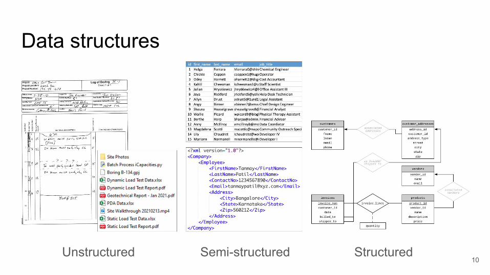
Data structures
Structured10
Semi-structuredUnstructured

DIGGS● Data Interchange for Geotechnical and Geoenvironmental
Specialists
● GML (XML-based) geospatial standard schema for the transfer of geotechnical and geoenvironmental data
● Enter data once, use anywhere DIGGS is supported
● Backed by ASCE, FHWA
11
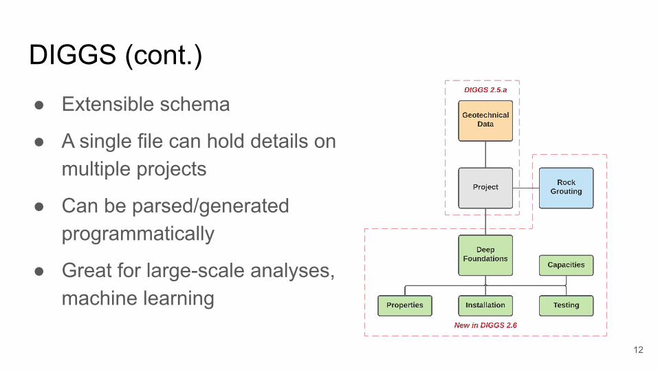
DIGGS (cont.)
● Extensible schema
● A single file can hold details on multiple projects
● Can be parsed/generated programmatically
● Great for large-scale analyses, machine learning
12

Bridge foundation design challenges● Wide scatter in nominal vs interpreted
capacities
● Semi-empirical, empirical design methods, based on the behavior of a few dozen piles
● Experience from past projects is transferred through people, not data, and often lost
● Missing the data structure, tools and methods to analyze at scale
13

Hypothesis
Can advanced analytics workflows lead to:● Accurate interpreted capacity● Reliable calculated capacity● Case-based design
14
RnNominal Capacity
RmInterpreted Capacity
i.e. 4,000 tons 1,000 - 16,000 tons
Rn ≈ Rm
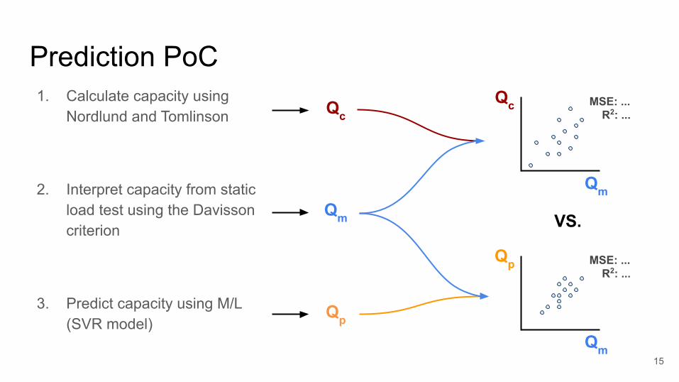
Prediction PoC
15
1. Calculate capacity using Nordlund and Tomlinson
2. Interpret capacity from static load test using the Davisson criterion
3. Predict capacity using M/L (SVR model)
Qc
Qm
Qp
Qc
Qm
Qp
Qm
VS.
MSE: ... R2: ...
MSE: ... R2: ...

Feature Selection
16
SOIL PILE1. Soil type (sand, clay, mixed) -
categorical
2. Average N count - numerical*
* intentional oversimplification; not ideal, but the quality of the available soil data does not justify the additional computational effort of using a layered system
1. Pile material (steel, concrete, composite) - categorical
2. Pile end (open/closed) - categorical
3. Cross sectional area - numerical
4. Circumference - numerical
5. Length - numerical
Three (3) categorical and four (4) numerical features

Results
17
● MSE reduced by a factor of 17 (62,566 kips)
● MPE improved by a factor of 2 (-47.78% to -25.7%)
● Absolute MPE reduced (76.3% to 42.3%)
● Test R2 was 0.6 (or 60%). The model yields errors that are 45% smaller than those of a constant-only model, on average. An improvement on errors by a factor of 9. Results of predicted capacity compared to measured capacity. Absolute MPE with
real-value MPE in parentheses (RHS legend)
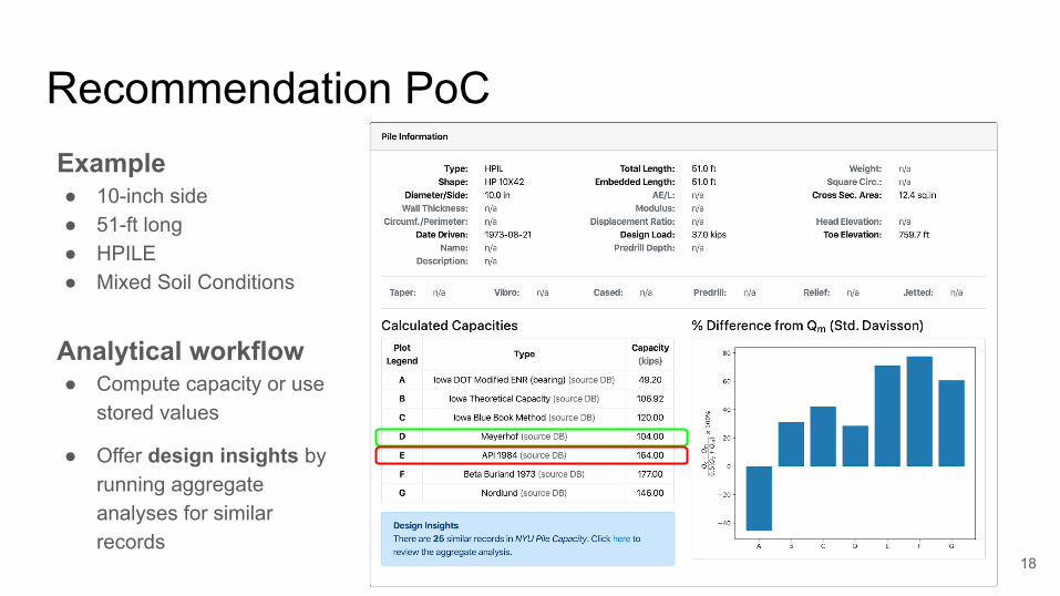
Recommendation PoC
18
Example● 10-inch side● 51-ft long● HPILE ● Mixed Soil Conditions
Analytical workflow● Compute capacity or use
stored values
● Offer design insights by running aggregate analyses for similar records

In conclusion● Reducing the inherent complexity of data management and analysis
enables interactivity and flexibility to investigate new areas
● Hypothesis is confirmed: more/better data and advanced analytics can lead to better bridge foundation designs
● There is no AI without high-quality, well-structured data
● Identify and empower citizen data scientists within your organization
● Get leadership on board and seek the advice of experts
19

Looking ahead● Proof of concept (PoC) studies on AI are excellent, and there is
an increasing number of them
● As AI is adopted and becomes more mature in our field, the focus will be on reliable applications rather than PoC
● Industry leaders will eventually compete on AI, and decision makers at the state/federal level might have to step in to set standards
20

Evaluating the Ultimate Pile Capacity from Cone Penetration Test (CPT) Data using Artificial Neural Network
Murad Abu-Farsakh, Ph.D., P.E., F-ASCEMd. Ariful Mojumder, Former MS Student
Louisiana Transportation Research CenterLouisiana State University
Baton Rouge, Louisiana
Webinar: Artificial Intelligence and Bridge Foundation Design
June 22, 2021

PRESENTATION OUTLINE
2
Introduction Objectives of the study Cone Penetration Test Overview of ANN Evaluation of Ultimate Pile Capacity from CPT Data Pile Load Tests Database Development of Neural Network Model Results of ANN Modeling Sensitivity Analysis of ANN model Inputs Comparison with Traditional Pile-CPT Methods Limitations of Study Conclusions

INTRODUCTION
Over the years, many analytical and empirical pile design methods weredeveloped [e.g., Static analysis methods using total or effective stresses (α, β, γ),Methods based on SPT data, Methods based on CPT] for different soil typesbased on lab or in-situ field test data.
These methods usually relate the pile capacity to different soil properties, whichare evaluated from laboratory and/or in-situ field tests that include soilborings/layering, undrained shear strength, friction angle, soil classification, etc.
Conducting laboratory tests is expensive and time consuming.
3

INTRODUCTION
Many direct pile-CPT methods were developed in the last few decades toestimate the ultimate pile capacity form CPT data (qt,fs), such as: Schmertmann,De Ruiter and Beringen, LCPC (Laboratoire Central des Ponts et Chaussees),probabilistic, UF (University of Florida) and many other CPT methods.
Most of the pile design methods involve several correlation assumptions andjudgments in selecting the proper correlation coefficients, which can influencethe calculation of ultimate pile capacity, that can result in inconsistent accuracyof pile capacity for different soil/pile conditions.
4

INTRODUCTION
To resolve the shortcoming in traditional direct pile-CPT methods, the ANNconcept can be introduced to develop models to estimate the pile capacity fromCPT data, since it does not need any correlation assumptions or judgements.
The ANN method usually learns from previous cases/instances and trains byusing special mathematical algorithms.
The developed ANN models are expected to yield better and consistent accuracyin estimating the ultimate pile capacity from CPT data.
5

OBJECTIVES OF THE STUDY
6
Explore the applicability of ANN in predicting the ultimate axial capacity ofpiles from CPT data.
Evaluate the relative importance of different input parameters, e.g. qt, fs,embedment pile length, L, and pile width, B.
Compare the ANN results with the well-performed direct pile-CPT methods.
Evaluate the ANN models within the context of LRFD reliability analysis todemonstrate their accuracy and bolster their reliability and feasibility.

CONE PENETRATION TEST (CPT)
7Cone Tip Resistance, qc
Slee
ve F
rict
ion,
f s
Penetration Rate: 2 cm/sec
Base area = 10 cm2
Sleeve area = 150 cm2
Cone angle = 60o
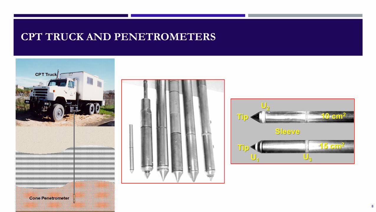
CPT TRUCK AND PENETROMETERS
8
Tip
Tip
Sleeve
U1
U2
U3
10 cm2
15 cm2
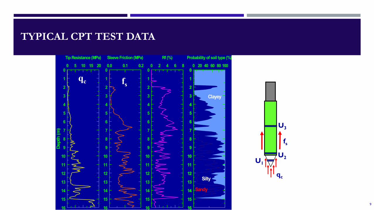
TYPICAL CPT TEST DATA
9
0
1
2
3
4
5
6
7
8
9
10
11
12
13
14
15
16
Dept
h (m
)0 5 10 15 20
Tip Resistance (MPa)
0
1
2
3
4
5
6
7
8
9
10
11
12
13
14
15
16
0.0 0.1 0.2
Sleeve Friction (MPa)
0
1
2
3
4
5
6
7
8
9
10
11
12
13
14
15
16
0 2 4 6 8
Rf (%)
0
1
2
3
4
5
6
7
8
9
10
11
12
13
14
15
16
0
1
2
3
4
5
6
7
8
9
10
11
12
13
14
15
16
0 20 40 60 80 100
Probability of soil type (%)
Sandy
Silty
Clayey
qc fs
qc
fs
U3
U2U1

TYPICAL CPT TEST DATA
10
qc fc
qt = qc + u2 (1 - a)a = An/Ac
qt = corrected cone resistanceqc = measured cone resistancea = effective cone area ratioAn= cross-sectional area of the load cellAc = area projected by the cone
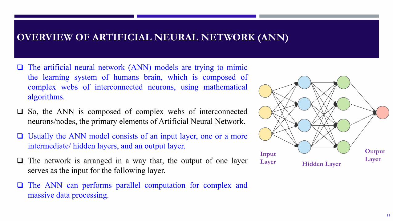
OVERVIEW OF ARTIFICIAL NEURAL NETWORK (ANN)
11
The artificial neural network (ANN) models are trying to mimicthe learning system of humans brain, which is composed ofcomplex webs of interconnected neurons, using mathematicalalgorithms.
So, the ANN is composed of complex webs of interconnectedneurons/nodes, the primary elements of Artificial Neural Network.
Usually the ANN model consists of an input layer, one or a moreintermediate/ hidden layers, and an output layer.
The network is arranged in a way that, the output of one layerserves as the input for the following layer.
The ANN can performs parallel computation for complex andmassive data processing.
Input Layer Hidden Layer
Output Layer
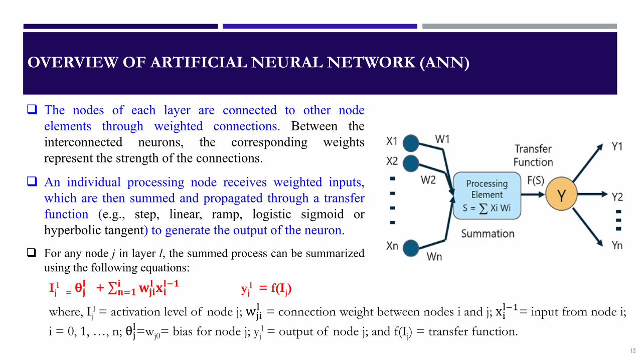
OVERVIEW OF ARTIFICIAL NEURAL NETWORK (ANN)
12
The nodes of each layer are connected to other nodeelements through weighted connections. Between theinterconnected neurons, the corresponding weightsrepresent the strength of the connections.
An individual processing node receives weighted inputs,which are then summed and propagated through a transferfunction (e.g., step, linear, ramp, logistic sigmoid orhyperbolic tangent) to generate the output of the neuron.
For any node j in layer l, the summed process can be summarizedusing the following equations:
Ijl
= 𝛉𝛉𝐣𝐣𝐥𝐥 + ∑𝐧𝐧=𝟏𝟏𝐢𝐢 𝐰𝐰𝐣𝐣𝐢𝐢𝐥𝐥 𝐱𝐱𝐢𝐢𝐥𝐥−𝟏𝟏 yj
l = f(Ij)
where, Ijl = activation level of node j; wji
l = connection weight between nodes i and j; xil−1= input from node i; i = 0, 1, …, n; θjl=wj0= bias for node j; yj
l = output of node j; and f(Ij) = transfer function.

OVERVIEW OF ARTIFICIAL NEURAL NETWORK (ANN)
13
The difference between the obtained output and the target output is the Error, E
E = ½(OutputTarget− Output obatined )2
The Error is then distributed backward through the weights starting from theoutput layer towards the input layer.
The weights, w, are then adjusted with respect to the corresponding error asfollows:
wnew = w - ƞ*𝝏𝝏𝝏𝝏𝝏𝝏𝐰𝐰
, ƞ is the learning rate
The network propagation is repeated with the updated weights until theobtained output is close enough to the target output (within acceptabletolerance).
OVERVIEW OF ARTIFICIAL NEURAL NETWORK (ANN)
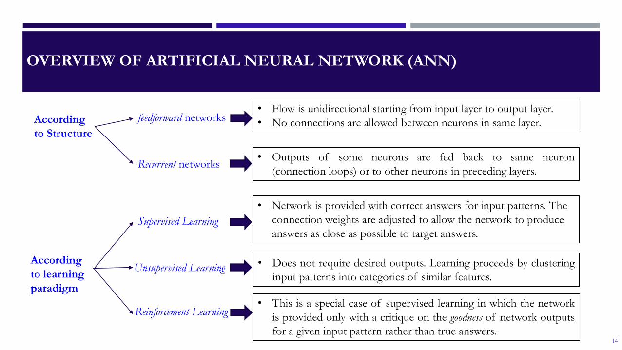
14
According to learning paradigm
According to Structure
feedforward networks
Recurrent networks
• Flow is unidirectional starting from input layer to output layer.• No connections are allowed between neurons in same layer.
• Outputs of some neurons are fed back to same neuron(connection loops) or to other neurons in preceding layers.
Supervised Learning
Unsupervised Learning
• Network is provided with correct answers for input patterns. The connection weights are adjusted to allow the network to produce answers as close as possible to target answers.
• Does not require desired outputs. Learning proceeds by clusteringinput patterns into categories of similar features.
Reinforcement Learning• This is a special case of supervised learning in which the network
is provided only with a critique on the goodness of network outputsfor a given input pattern rather than true answers.
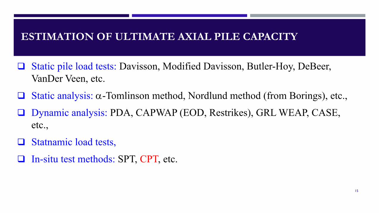
ESTIMATION OF ULTIMATE AXIAL PILE CAPACITY
15
Static pile load tests: Davisson, Modified Davisson, Butler-Hoy, DeBeer, VanDer Veen, etc.
Static analysis: α-Tomlinson method, Nordlund method (from Borings), etc.,
Dynamic analysis: PDA, CAPWAP (EOD, Restrikes), GRL WEAP, CASE, etc.,
Statnamic load tests,
In-situ test methods: SPT, CPT, etc.
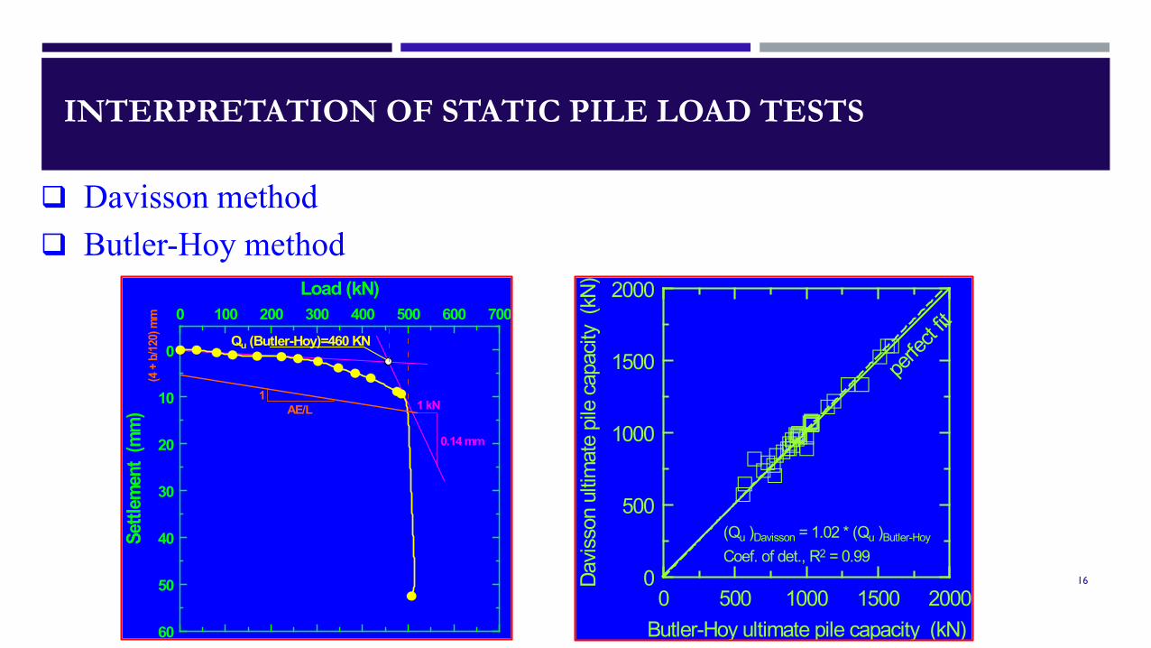
INTERPRETATION OF STATIC PILE LOAD TESTS
16
0
10
20
30
40
50
60
Settl
emen
t (m
m)
0 100 200 300 400 500 600 700Load (kN)
Qu (Butler-Hoy)=460 KN
1 kN
0.14 mm
1AE/L
(4 +
b/12
0) m
m
0 500 1000 1500 2000Butler-Hoy ultimate pile capacity (kN)
0
500
1000
1500
2000
Davis
son
ultim
ate
pile
cap
acity
(kN
)
(Qu )Davisson = 1.02 * (Qu )Butler-Hoy Coef. of det., R2 = 0.99
perfe
ct fit
Davisson method Butler-Hoy method

INTERPRETATION OF STATIC PILE LOAD TESTS
17
0
10
20
30
40
50
60
Settl
emen
t (m
m)
0 100 200 300 400 500 600 700Load (kN)
Qu (Butler-Hoy)=460 KN
1 kN
0.14 mm
1AE/L
(4 +
b/12
0) m
m
0 500 1000 1500 2000Butler-Hoy ultimate pile capacity (kN)
0
500
1000
1500
2000
Davis
son
ultim
ate
pile
cap
acity
(kN
)
(Qu )Davisson = 1.02 * (Qu )Butler-Hoy Coef. of det., R2 = 0.99
perfe
ct fit
Davisson method Butler-Hoy method
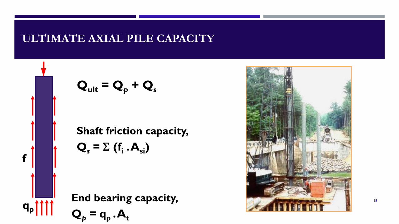
ULTIMATE AXIAL PILE CAPACITY
18End bearing capacity, Qp = qp . At
Shaft friction capacity, Qs = Σ (fi . Asi)
Qult = Qp + Qs
f
qp

CONE PENETRATION VERSUS PILE
19
qc
f s
f
qp
Qult
Due to similarity between cone and pile, the cone can be considered as a simple mini pile.
fs can be correlated to f, qc can be correlated to qp

ESTIMATION OF PILE CAPACITY FROM CPT DATA
20
Indirect Approach– Use the CPT data (qc, fs) to evaluate the soil strength parameters
strength parameters, such as undrained shear strength (Su) for clay and angle of internal friction (φ) for sand, from CPT data → input for Static Analysis Methods.
Direct Approach✓Evaluate pile capacity directly from CPT data (qc, fs)– The pile unit toe resistance (qp) is evaluated from the cone tip resistance (qc)
profile,– The pile unit shaft resistance (f) is evaluated either from the sleeve friction
(fs) or from the cone tip resistance (qc) profiles.

ESTIMATION OF PILE CAPACITY FROM CPT
21
0
5
10
15
20
25
30
35
40
Dept
h (m
)0 5 101520
Tip resistanceqc (MPa)
0 0.1 0.2
Sleeve friction fs (MPa)
0 2 4 6 810
Friction ratioRf (%)
0
5
10
15
20
25
30
35
40
0
5
10
15
20
25
30
35
40
qca2
qca1
qca3
qca5
qca6
qca4
fsa3
fsa4
fsa5
fsa6
fsa1
Fsa2
Pile
fc
qc
100%cf
c
fR .q
=

ESTIMATION OF PILE CAPACITY FROM CPT DATA
22
qca
fsa
qp
f
Cone data
Clay
Silt
Sand
Soil Type
f
qp
fs
qc
Pile Parameters

DIRECT PILE-CPT DESIGN METHODS
23
1- Schmertmann
2- De Ruiter and Beringen
3- LCPC (Bustamante and Gianeselli)
4- Tumay and Fakhroo
5- Aoki and De Alencar
6- Price and Wardle
7- Philipponnat
8- Penpile
9- NGI
10- ICP
11- UWA
12- CPT2000
13- Fugro
14- Purdue
15- Probabilistic
16- UF
17- Togliani
18- Zhou
19- ERTC3
20- German
21- Eurocode
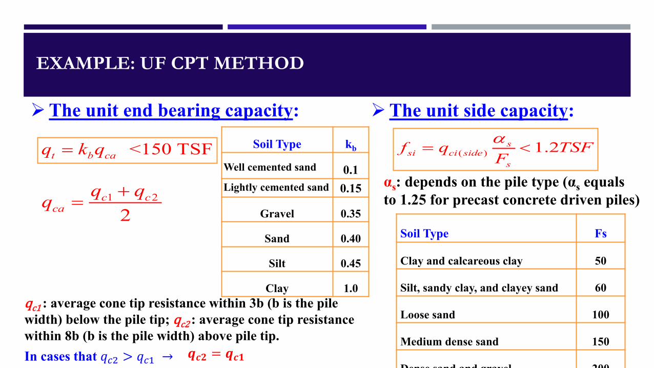
EXAMPLE: UF CPT METHOD
The unit end bearing capacity:
( ) 1.2ssi ci side
s
f q TSFFα
= <
αs: depends on the pile type (αs equals to 1.25 for precast concrete driven piles)
Soil Type Fs
Clay and calcareous clay 50
Silt, sandy clay, and clayey sand 60
Loose sand 100
Medium dense sand 150
Dense sand and gravel 200
The unit side capacity:Soil Type kb
Well cemented sand 0.1Lightly cemented sand 0.15
Gravel 0.35
Sand 0.40
Silt 0.45
Clay 1.0
<150 TSFt b caq k q=
1 2 2
c cca
q qq +=
qc1 : average cone tip resistance within 3b (b is the pile width) below the pile tip; qc2 : average cone tip resistance within 8b (b is the pile width) above pile tip.In cases that 𝑞𝑞𝑐𝑐𝑐 > 𝑞𝑞𝑐𝑐1 → 𝒒𝒒𝒄𝒄𝟐𝟐 = 𝒒𝒒𝒄𝒄𝟏𝟏

PILE LOAD TEST DATABASE
25
The database consists of eighty (80) precast prestressed concrete(PPC) piles of different sizes and lengths were collected from 34different project sites across the state of Louisiana.
All the piles were square piles loaded to failure under static loadtests. The corresponding CPT tests were conducted close to eachtest pile. The pile lengths range from 36 ft. to 200 ft., and the pilewidths range from 14 in. to 36 in.
The pile load tests were performed based on quick load test asdescribed by ASTM D1143 testing procedure. The tests wereperformed 14 days after pile driving , partially accounted for pilesetup.
Davisson interpretation criteria was used to estimate the ultimatepile capacity from the load-settlement curve for each pile load test.

DEVELOPMENT OF NEURAL NETWORK MODEL
Model Input Parameters The proper selection of input variables is very important for developing ANN models,
since it has significant impact on the performance of the ANN models.
Based on prior knowledge from literature, the selected input variables were: pileembedment length, L, pile width, B, corrected cone tip resistance, qt, and cone sleevefriction, fs. The ultimate pile capacity, qt, was the only output.
There are some other factors, such as the pile installation method, pile type, whether thepile tip is open or closed, shape of pile cross-section, etc. These factors were ignored inthis study since all the tested piles were square precast prestressed concrete (PPC) drivenpile with closed tip.

DEVELOPMENT OF NEURAL NETWORK MODEL
27
Model Input Parameters The soil properties along the shaft of the pile varies with depth. To account for this variability, the embedded length of the piles
was divided into five equal segments (layers). For each division,the average qt, avg and fs,avg were determined as follow:
qt, avg = ∑𝒒𝒒𝒕𝒕𝒕𝒕 𝒁𝒁𝒕𝒕∑𝒁𝒁𝒕𝒕
, fs, avg = ∑𝒇𝒇𝐬𝐬𝐢𝐢 𝒁𝒁𝒕𝒕∑𝒁𝒁𝒕𝒕
For calculating the pile end bearing capacity, the averagecorrected tip resistance, qt-tip, was calculated for two cases ofinfluence zone: 4B below to 4B above pile toe, and 4B below to8B above pile toe, in order to find the best results.

DEVELOPMENT OF NEURAL NETWORK MODEL
28
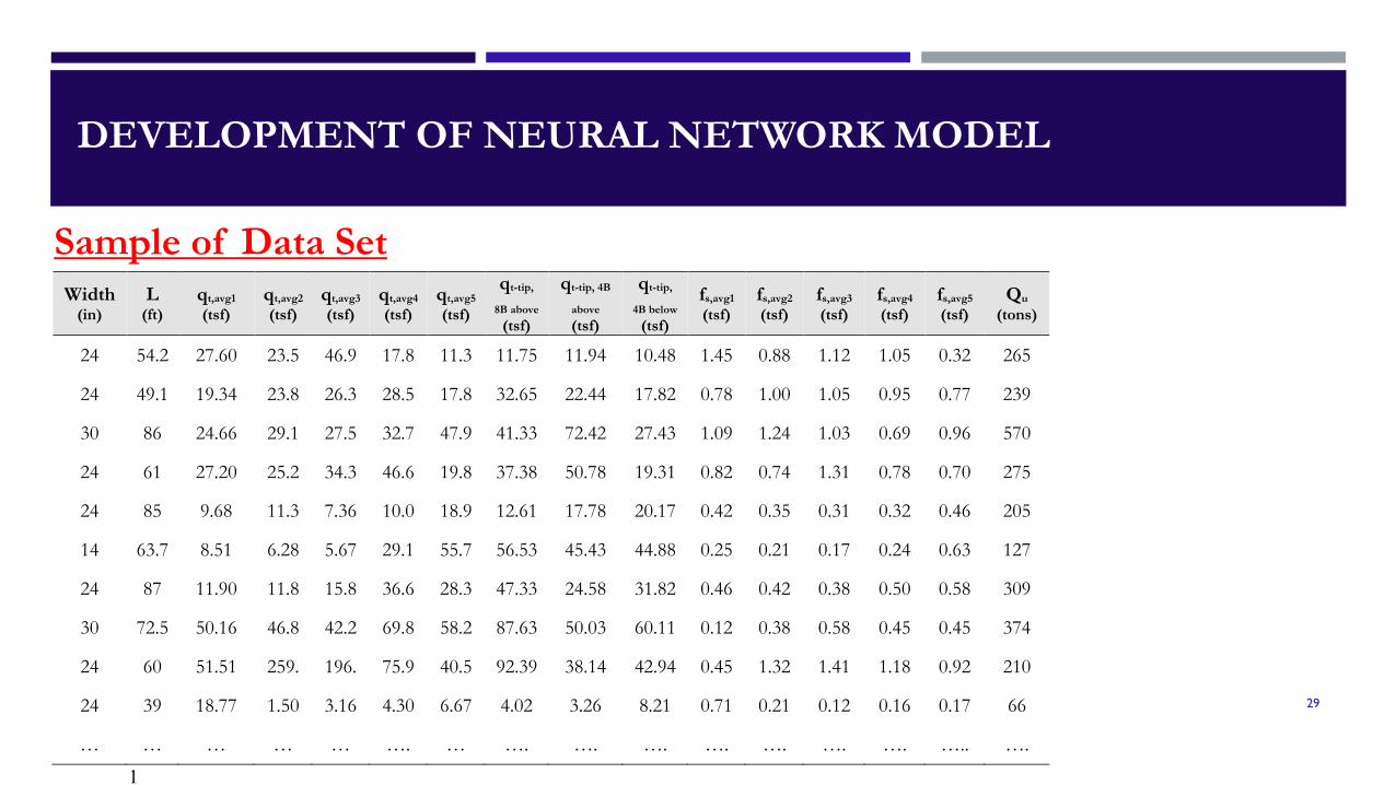
Model Input Parameters The final selection of ANN input parameters were: (1) Pile embedment depth, L, (2) Pile
width, B, (3) qt, avg 1, (4) qt, avg 2, (5) qt, avg 3, (6) qt, avg 4, (7) qt, avg 5, (8) fs, avg 1, (9) fs, avg 2,(10) fs, avg 3, (11) fs, avg 4, (12) fs, avg 5, (13) qt-tip, 4B/8B above, (14) qt-tip, 4B below.
These inputs parameters were arranged in six different combinations (6 ANN ModelTypes) to determine the ANN model(s) that yields the best performance in terms ofestimating the measured ultimate pile capacity of driven PPC piles.
DEVELOPMENT OF NEURAL NETWORK MODEL
29
Sample of Data Set
1
Width (in)
L (ft)
qt,avg1 (tsf)
qt,avg2 (tsf)
qt,avg3 (tsf)
qt,avg4 (tsf)
qt,avg5 (tsf)
qt-tip,
8B above (tsf)
qt-tip, 4B
above (tsf)
qt-tip,
4B below (tsf)
fs,avg1 (tsf)
fs,avg2 (tsf)
fs,avg3 (tsf)
fs,avg4 (tsf)
fs,avg5 (tsf)
Qu (tons)
24 54.2 27.60 23.5 46.9 17.8 11.3 11.75 11.94 10.48 1.45 0.88 1.12 1.05 0.32 265
24 49.1 19.34 23.8 26.3 28.5 17.8 32.65 22.44 17.82 0.78 1.00 1.05 0.95 0.77 239
30 86 24.66 29.1 27.5 32.7 47.9 41.33 72.42 27.43 1.09 1.24 1.03 0.69 0.96 570
24 61 27.20 25.2 34.3 46.6 19.8 37.38 50.78 19.31 0.82 0.74 1.31 0.78 0.70 275
24 85 9.68 11.3 7.36 10.0 18.9 12.61 17.78 20.17 0.42 0.35 0.31 0.32 0.46 205
14 63.7 8.51 6.28 5.67 29.1 55.7 56.53 45.43 44.88 0.25 0.21 0.17 0.24 0.63 127
24 87 11.90 11.8 15.8 36.6 28.3 47.33 24.58 31.82 0.46 0.42 0.38 0.50 0.58 309
30 72.5 50.16 46.8 42.2 69.8 58.2 87.63 50.03 60.11 0.12 0.38 0.58 0.45 0.45 374
24 60 51.51 259. 196. 75.9 40.5 92.39 38.14 42.94 0.45 1.32 1.41 1.18 0.92 210
24 39 18.77 1.50 3.16 4.30 6.67 4.02 3.26 8.21 0.71 0.21 0.12 0.16 0.17 66
… … … … … …. … …. …. …. …. …. …. …. ….. ….

DEVELOPMENT OF NEURAL NETWORK MODEL
30
Types of ANN Models Types of ANN Model Input Parameters
Type 1 (1) Pile embedment depth, L, (2) Pile width, D, (3) qt, avg 1, (4) qt, avg 2, (5) qt, avg 3, (6) qt, avg 4, (7) qt, avg 5, (8) qt-tip, 4B above, (9) qt-tip, 4B below
Type 2 (1) Pile embedment depth, L, (2) Pile width, D, (3) qt, avg 1, (4) qt, avg 2, (5) qt, avg 3, (6) qt, avg 4, (7) qt, avg 5, (8) qt-tip, 8B above, (9) qt-tip, 4B below
Type 3 (1) Pile embedment depth, L, (2) Pile width, D (3) fs, avg 1, (4) fs, avg 2, (5) fs, avg 3, (6) fs, avg 4, (7) fs, avg 5, (8) qt-tip, 4B above, (9) qt-tip, 4B below
Type 4 (1) Pile embedment depth, L, (2) Pile width, D (3) fs, avg 1, (4) fs, avg 2, (5) fs, avg 3, (6) fs, avg 4, (7) fs, avg 5, (8) qt-tip, 8B above, (9) qt-tip, 4B below
Type 5 (1) Pile embedment depth, L, (2) Pile width, D, (3) qt, avg 1, (4) qt, avg 2, (5) qt, avg 3, (6) qt, avg 4, (7) qt, avg 5, (8) fs, avg 1, (9) fs, avg 2, (10) fs, avg 3,
(11) fs, avg 4, (12) fs, avg 5, (13) qt-tip, 4B above, (14) qt-tip, 4B below
Type 6 (1) Pile embedment depth, L, (2) Pile width, D, (3) qt, avg 1, (4) qt, avg 2, (5) qt, avg 3, (6) qt, avg 4, (7) qt, avg 5, (8) fs, avg 1, (9) fs, avg 2, (10) fs, avg 3, (11) fs,
avg 4, (12) fs, avg 5, (13) qt-tip, 8B above, (14) qt-tip, 4B below

DEVELOPMENT OF NEURAL NETWORK MODEL
31
Training of ANN Models Training of ANN model refers to the process of initializing a network through the deployment of initial
values and then optimizing the connection weights in order to obtain global minima instead of a local one.
A widely used method to obtain the optimum weights is the back-propagation algorithm or the gradientdescent method. However, the convergence is sometimes slower and requires lots of iterations. Therefore,a faster Quasi-Newton method was used in this work to optimize weights for the ANN model.
Stopping Criteria of Training Process It is important to determine when to stop the training process. In this study, the cross-validation method
was implemented where data was divided into three sets: 70% training, 12% testing and 18% validation.
The function of training set is to re-adjust the connection weights. The testing set judges the capability ofthe model to be generalized, through evaluating the performance of the model at different stages of thetraining process. When an increase in error is detected, the training process is stopped. The validation setensures the model’s ability to be generalized in a robust way within the limits of training data.
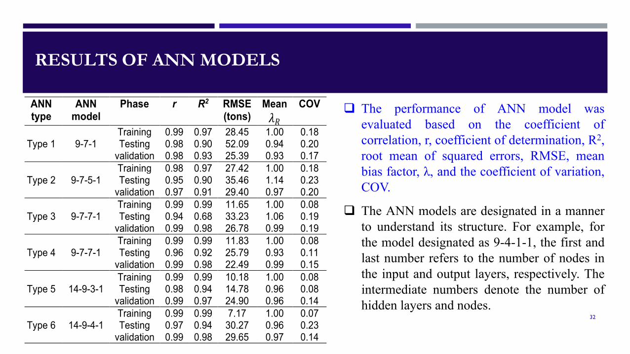
RESULTS OF ANN MODELS
32
ANN type
ANN model
Phase r R2 RMSE (tons)
Mean 𝜆𝜆𝑅𝑅
COV
Type 1 9-7-1 Training 0.99 0.97 28.45 1.00 0.18 Testing 0.98 0.90 52.09 0.94 0.20
validation 0.98 0.93 25.39 0.93 0.17
Type 2 9-7-5-1 Training 0.98 0.97 27.42 1.00 0.18 Testing 0.95 0.90 35.46 1.14 0.23
validation 0.97 0.91 29.40 0.97 0.20
Type 3 9-7-7-1 Training 0.99 0.99 11.65 1.00 0.08 Testing 0.94 0.68 33.23 1.06 0.19
validation 0.99 0.98 26.78 0.99 0.19
Type 4 9-7-7-1 Training 0.99 0.99 11.83 1.00 0.08 Testing 0.96 0.92 25.79 0.93 0.11
validation 0.99 0.98 22.49 0.99 0.15
Type 5 14-9-3-1 Training 0.99 0.99 10.18 1.00 0.08 Testing 0.98 0.94 14.78 0.96 0.08
validation 0.99 0.97 24.90 0.96 0.14
Type 6 14-9-4-1 Training 0.99 0.99 7.17 1.00 0.07 Testing 0.97 0.94 30.27 0.96 0.23
validation 0.99 0.98 29.65 0.97 0.14
The performance of ANN model wasevaluated based on the coefficient ofcorrelation, r, coefficient of determination, R2,root mean of squared errors, RMSE, meanbias factor, λ, and the coefficient of variation,COV.
The ANN models are designated in a mannerto understand its structure. For example, forthe model designated as 9-4-1-1, the first andlast number refers to the number of nodes inthe input and output layers, respectively. Theintermediate numbers denote the number ofhidden layers and nodes.
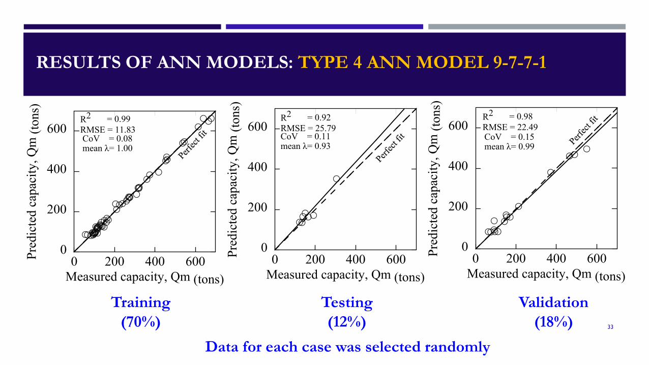
RESULTS OF ANN MODELS: TYPE 4 ANN MODEL 9-7-7-1
33
Training(70%)
Testing(12%)
Validation(18%)
R2 = 0.98RMSE = 22.49CoV = 0.15mean λ= 0.99
0 200 400 600Measured capacity, Qm (tons)
0
200
400
600
Pred
icte
d ca
paci
ty, Q
m (t
ons)
R2 = 0.92RMSE = 25.79CoV = 0.11mean λ= 0.93
0 200 400 600Measured capacity, Qm (tons)
0
200
400
600
Pred
icte
d ca
paci
ty, Q
m (t
ons)
R2 = 0.99RMSE = 11.83CoV = 0.08mean λ= 1.00
0 200 400 600Measured capacity, Qm (tons)
0
200
400
600
Pred
icte
d ca
paci
ty, Q
m (t
ons)
Data for each case was selected randomly

RESULTS OF ANN MODELS: TYPE 5 ANN MODEL 14-9-3-1
34
Training(70%)
Testing(12%)
Validation(18%)
Data for each case was selected randomly
R2 = 0.97RMSE = 24.90CoV = 0.14mean λ= 0.96
0 200 400 600Measured capacity, Qm (tons)
0
200
400
600
Pred
icte
d ca
paci
ty, Q
p (to
ns)
R2 = 0.94RMSE = 14.78CoV = 0.08mean λ= 0.96
0 200 400 600Measured capacity, Qm (tons)
0
200
400
600
Pred
icte
d ca
paci
ty, Q
p (to
ns)
R2 = 0.99RMSE = 10.18CoV = 0.08mean λ= 1.00
0 200 400 600Measured capacity, Qm (tons)
0
200
400
600
Pred
icte
d ca
paci
ty, Q
p (to
ns)

SENSITIVITY ANALYSIS (14-9-3-1)
35
CPT Input Variables The Relative Importance of the
Input Variables (%) Embedment length of pile, L 14.8 Width of pile, B 14.1 qt-tip, 4B above 19.0 qt-tip, 4B below 22.8 qt-avg along the pile shaft 12.9 fs-avg along the pile shaft 16.4

COMPARISON WITH TRADITIONAL PILE-CPT METHODS
36
Amirmojahedi and Abu-Farsakh (2019) evaluated 21 traditional direct pile-CPT methods forestimating the ultimate pile capacity form CPT data (qt,fs) using a database of 80 pile load tests,and ranked LCPC, probabilistic and UF methods as the best three performed pile-CPT methods.
The best-performed ANN models ( 9-7-7-1, 14-9-3-1) developed in this study were comparedwith the aforementioned three pile-CPT methods.
The comparison clearly shows that, the ANN models outperform these three pile-CPT methodsin almost all evaluation criteria. Especially the RMSE value seems to be much higher in theconventional methods.

EVALUATION AND COMPARISON BASED ON LRFD ANALYSIS
37
LRFD analysis help to grasp a better understanding of efficiency of the developed ANN models.
First Order Reliability Method (FORM) was used to calibrate the LRFD resistance factors.
QD/QL equal to 3 (specified by AASHTO LRFD)
A target reliability (βT) of 2.33 was selected
Bias factor, 𝜆𝜆𝑅𝑅 = Q𝑚𝑚Q𝑝𝑝

LIMITATIONS OF STUDY
38
The data set represents clayey soils in Louisiana. Thus, the proposedANN models should perform well for clayey soils in Louisiana, andother locations with similar geological conditions.
The range of qt should be (0-300) tsf, the range of fs should be (0-3.2)tsf and B should be <36 in, and the range of Qt should be (0-678) tons.
Recommended for squared PPC driven piles only.The developed ANN models should be used to predict the data for
unknown sites without further training. If it is trained again on the sametraining data, the prediction capability might not remain the same.
CONCLUSIONS
39
All the developed ANN model types were able to estimate the measured ultimatecapacity of the 80 pile load tests with good to excellent accuracy.
However, Type 4 ANN model 9-7-7-1 (λ = 0.99, RMSE = 22.49, COV = 0.15) and Type5 ANN model 14-9-3-1 (λav = 0.96, RMSEav = 21.53, COVav = 0.12) showed betterperformance.
Using the combination of qt, avg, and fs, avg, to evaluate the pile’s skin friction gives betterANN prediction models.
Sensitivity analysis showed that the qt-tip,4B below, has relatively the highest importanceinput parameter.
fs-avg, has higher importance than qt-avg along the shaft in evaluating pile skin friction.
CONCLUSIONS
40
The comparison with LCPC, probabilistic, and UF methods clearly showed that theANN models outperformed the traditional pile-CPT methods with lower RMSE andlower COV.
The evaluation and comparison based on LRFD reliability analysis demonstrated higherresistant factors and superior efficiencies for the ANN models.
Finally, the ANN models use data and previous experience and training withoutincorporating any assumption or hypothesis. Besides, the ANN models can becontinuously updated with time to achieve more accurate estimation results, whenevernew pile load test data are available.

41
THANK YOU!!

Moderated by: Sharid Amiri, California DOT
Today’s Panelists
#TRBwebinar
Nick Machairas, Haley & Aldrich
Murad Abu-Farsakh,Louisiana State University

TRB’s New Podcast!• Have you heard that we have a new
podcast, TRB’s Transportation Explorers?• Listen on our website or subscribe
wherever you listen to podcasts!
#TRBExplorers

Get Involved with TRB
#TRBwebinarReceive emails about upcoming TRB webinarshttps://bit.ly/TRBemails
Find upcoming conferenceshttp://www.trb.org/Calendar

Get Involved with TRB
Be a Friend of a Committee bit.ly/TRBcommittees– Networking opportunities
– May provide a path to Standing Committee membership
Join a Standing Committee bit.ly/TRBstandingcommittee
Work with CRP https://bit.ly/TRB-crp
Update your information www.mytrb.org
#TRBwebinar
Getting involved is free!