the functional renormalization group method an … · the callan-symanzik regulator: rk(p) = k2...

The Functional Renormalization Group Method –An Introduction

A. Wipf

Theoretisch-Physikalisches Institut, FSU Jena

Saalburg Sommer School – Wolfersdorf

11. September 2015

Andreas Wipf (FSU Jena) The Functional Renormalization Group Method – An Introduction11. September 2015 1 / 60

1 Introduction

2 Scale-dependent Functionals

3 Derivation of Flow Equations

4 Functional Renormalization in QM

5 Scalar Field Theories

6 O(N) Models


9Andreas Wipf (FSU Jena) The Functional Renormalization Group Method – An Introduction11. September 2015 3 / 60

Introduction

implementation of the renormalization group ideafor continuum field theoryfunctional methods + renormalization groupscale-dependent Schwinger functional Wk [j]scale-dependent effective action Γk [ϕ]

conceptionally simple, technically demanding flow equationsscale parameter k = adjustable screw of microscopelarge values of a momentum scale k : high resolutionlowering k : decreasing resolution of the microscope(known) microscopic laws −→ complex macroscopic phenomenanon-perturbative


Wk [j] obeys Polchinski flow equationΓk [ϕ] obeys Wetterich flow equationflow from classical action S[ϕ] to effective action Γ[ϕ]

applied to variety of physical systemsI strong interactionI electroweak phase transitionI asymptotic safety scenarioI condensed matter systen

e.g. Hubbard model, liquid He4, frustrated magnets,superconductivity . . .

I effective models in nuclear physicsI ultra-cold atoms


Γk=Λ = S

Γk=0 = Γ

Theory space


1 K. Aoki, Introduction to the nonperturbative renormalization groupand its recent applications,Int. J. Mod. Phys. B14 (2000) 1249.

2 C. Bagnus and C. Bervillier, Exact renormalization groupequations: An introductionary review,Phys. Rept. 348 (2001) 91.

3 J. Berges, N. Tetradis and C. Wetterich, Nonperturbativerenormalization flow in quantum field theory and statisticalphysics,Phys. Rept. 363 (2002) 223.

4 J. Polonyi, Lectures on the functional renormalization groupmethods,Central Eur. J. Phys. 1 (2003) 1.

5 J. Pawlowski, Aspects of the functional renormalisation group,Annals Phys. 322 (2007) 2831.


1 H. Gies, Introduction to the functional RG and applications togauge theories,Lect. Notes Phys. 162, Springer, Berlin (2012) Renormalizationgroup and effective field theory approaches to many-bodysystems, ed. by A. Schwenk, J. Polonyi.

2 P. Kopietz, L. Bartosch and F. Schütz, Introduction to thefunctional renormalization group,Lect. Notes Phys. 798, Springer, Berlin (2010).

3 A. Wipf, Statistical Approach to Quantum Field TheoryLect. Notes Phys. 864, Springer, Berlin (2013).


Scale-dependent functionals

generating functional of (Euclidean) correlation functions

Z [j] =

∫Dφ e−S[φ]+(j,φ), (j , φ) =

∫ddx j(x)φ(x)

Schwinger functional W [j] = log Z [j]→ connected correlationfunctionseffective action = Legendre transform of W [j]

Γ[ϕ] = (j , ϕ)−W [j] with ϕ(x) = 〈φ(x)〉j =δW [j]δj(x)

→ one-particle irreducible correlation functionssolve for j[ϕ], insert into first equationΓ[ϕ]: encodes properties of QFT in most economic way


add scale-dependent IR-cutoff term ∆Sk to classical action infunctional integral→ scale-dependent generating functional

Zk [j] =

∫Dφ e−S[φ]+(j,φ)−∆Sk [φ] (1)

Scale-dependent Schwinger functional

Wk [j] = log Zk [j] (2)

regulator: quadratic functional with a momentum-dependent mass,

∆Sk [φ] =12

∫ddp

(2π)d φ∗(p)Rk (p)φ(p) ≡ 1

2

∫pφ∗(p)Rk (p)φ(p) ,

→ one-loop structure of flow equation


Conditions on cutoff function Rk(p)

should recover effective action for k → 0:

Rk (p)k→0−→ 0 for fixed p

should recover classical action at UV-scale Λ:

Rkk→Λ−→ ∞

regularization in the IR:

Rk (p) > 0 for p → 0


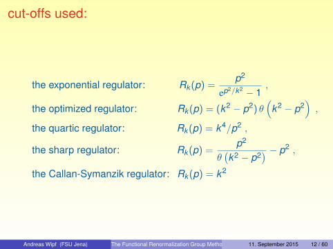
cut-offs used:

the exponential regulator: Rk (p) =p2

ep2/k2 − 1,

the optimized regulator: Rk (p) = (k2 − p2) θ(

k2 − p2),

the quartic regulator: Rk (p) = k4/p2 ,

the sharp regulator: Rk (p) =p2

θ(k2 − p2

) − p2 ,

the Callan-Symanzik regulator: Rk (p) = k2


exponential cutoff function and its derivative

p2

Rk

k∂kRk

k2 2k2

k2

2k2


Polchinski equation

partial derivative of Wk in (2) is given by

∂kWk [j] = −12

∫ddxddy 〈φ(x)∂kRk (x , y)φ(y)〉k

relates to connected two-point function

G(2)k (x , y) ≡ δ2Wk [j]

δj(x)δj(y)= 〈φ(x)φ(y)〉k − ϕ(x)ϕ(y)

Polynomial Polchinski equation

∂kWk = −12

∫ddxddy ∂kRk (x , y)G(2)

k (y , x)− ∂k ∆Sk [ϕ]

= −12

tr(∂kRk W ′′

k)− ∂k ∆Sk

[W ′

k]

(3)


Scale dependent effective action

average field of the cutoff theory with j

ϕ(x) =δWk [j]δj(x)

(4)

fixed source j → average field ϕ depends on cutofffixed average field→ source depends on cutoffmodified Legendre transformation:

Γk [ϕ] = (j , ϕ)−Wk [j]−∆Sk [ϕ] (5)

solve (4) for j = j[ϕ]→ use solution in (5)Γk not Legendre transform of Wk [j] for k > 0!Γk need not to be convex, but Γk→0 is convex


Derivation of Wetterich equation

vary effective average action

δΓk

δϕ(x)=

∫δj(y)

δϕ(x)ϕ(y) + j(x)−

∫δWk [j]δj(y)

δj(y)

δϕ(x)− δ∆Sk [ϕ]

δϕ(x)

terms chancel→ effective equation of motion

δΓk

δϕ(x)= j(x)− δ

δϕ(x)∆Sk [ϕ] = j(x)− (Rkϕ)(x) (6)

flow equation: ϕ fixed, j depends on scale, differentiate Γk

∂k Γk =

∫ddx ∂k j(x)ϕ(x)− ∂kWk [j]−

∫∂Wk [j]∂j(x)

∂k j(x)− ∂k ∆Sk [ϕ]


black terms cancel∂kWk [j]: only scale dependence of the parameters

∂k Γk = −∂kWk [j]− ∂k ∆Sk [ϕ]

= −∂kWk [j]− 12

∫ddxddy ϕ(x)∂kRk (x , y)ϕ(y)

use Polchinski equation→

∂k Γk =12

∫ddxddy ∂kRk (x , y) G(2)

k (y , x) (7)

second derivative of Wk vs. second derivative of Γk :

ϕ(x) =δWk [j]δj(x)

and j(x)(6)=

δΓk

δϕ(x)+

∫ddy Rk (x , y)ϕ(y)


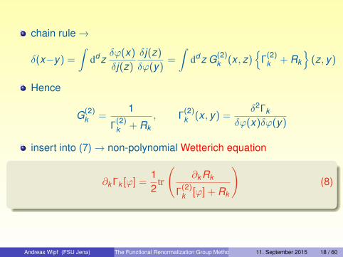
chain rule→

δ(x−y) =

∫ddz

δϕ(x)

δj(z)

δj(z)

δϕ(y)=

∫ddz G(2)

k (x , z){

Γ(2)k + Rk

}(z, y)

Hence

G(2)k =

1

Γ(2)k + Rk

, Γ(2)k (x , y) =

δ2Γk

δϕ(x)δϕ(y)

insert into (7)→ non-polynomial Wetterich equation

∂k Γk [ϕ] =12

tr

(∂kRk

Γ(2)k [ϕ] + Rk

)(8)


(finite) non-linear functional integro-differential equationfirst order in k ⇒ ’initial condition’ ΓΛ determines Γk

full propagator enters flow equationfinite and exact FRG flow equationsPolchinski: simple polynomial structurefavored in structural investigationsWetterich: second derivative in the denominatorstabilizes flow in (numerical) approachmainly used in explicit calculations.in practice: truncation = projection onto finite-dim. spacedifficult: error estimate for truncated flow→ improve truncation, optimize regulator, check stability


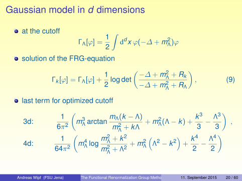
Gaussian model in d dimensions

at the cutoffΓΛ[ϕ] =

12

∫ddx ϕ(−∆+ m2

Λ)ϕ

solution of the FRG-equation

Γk [ϕ] = ΓΛ[ϕ] +12

log det(−∆+ m2

Λ + Rk

−∆+ m2Λ + RΛ

), (9)

last term for optimized cutoff

3d:1

6π2

(m3

Λ arctanmΛ(k − Λ)

m2Λ + kΛ

+ m2Λ(Λ− k) +

k3

3− Λ3

3

),

4d:1

64π2

(m4

Λ logm2

Λ + k2

m2Λ + Λ2

+ m2Λ

(Λ2 − k2

)+

k4

2− Λ4

2

)


Functional renormalization in QM

anharmonic oscillator

S[q] =

∫dτ(

12

q2 + V (q)

),

here LPA (local potential approximation)

Γk [q] =

∫dτ(

12

q2 + uk (q)

)(10)

low-energy approximationleading order in gradient expansionscale-dependent effective potential uk

neglected: higher derivative terms, mixed terms qnqm


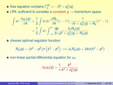
flow equation contains Γ(2)k = −∂2

τ + u′′k (q)

LPA: sufficient to consider a constant q → momentum space∫dτ

∂uk (q)

∂k=

12

∫dτdτ ′

∂Rk

∂k(τ − τ ′) 1

−∂2τ + u′′k (q) + Rk

(τ ′ − τ)

=12

∫dτ∫ ∞−∞

dp2π

∂kRk (p)

p2 + u′′k (q) + Rk (p)

choose optimal regulator function

Rk (p) = (k2 − p2) θ(

k2 − p2)

=⇒ ∂kRk (p) = 2kθ(k2 − p2)

non-linear partial differential equation for uk :

∂kuk (q) =1π

k2

k2 + u′′k (q)


minimum of uk (q) not ground state energydiffers by q-independent contributionfree particle limit fixes subtraction in flow equation

∂kuk (q) =1π

(k2

k2 + u′′k (q)− 1)

= −1π

u′′k (q)

k2 + u′′k (q)(11)

assume uΛ(q) even→ uk (q) evenpolynomial ansatz

uk (q) =∑

n=0,1,2...

1(2n)!

a2n(k) q2n ,


scale-dependent couplings a2n(k)

Insert into (11), compare coefficients of powers of q2

→ infinite set of coupled ode’s

da0

dk= −1

πa2∆0, ∆0 =

1k2 + a2

,

da2

dk= −k2

πa4∆2

0 ,

da4

dk= −

k2∆20

π

(a6 − 6a2

4∆0

),

da6

dk= −

k2∆20

π

(a8 − 30a4a6∆0 + 90a3

4∆20

),

......

initial condition: a2n at cutoff = parameters in classical potentialprojection onto space of polynomials up to given degree n


e.g. crude truncation a6 = a8 = · · · = 0: finite set of ode’suse standard notation

a0 = Ek , a2 = ω2k , a4 = λk and ∆0 =

1k2 + ω2

k,

⇒ truncated system of flow equations

dEk

dk= −

ω2kπ

∆0,dω2

kdk

= −k2λk

π∆2

0,dλk

dk=

6k2λ2k

π∆3

0

solve numerically (eg. with octave)initial conditions EΛ = 0, ωΛ = 1, varying λ at the cutoff scale→ scale-dependent couplings Ek and ω2

k

hardly change for k � ω

variation near typical scale k ≈ ω


k

Ek

.1

.2

.3

.4

.5

1 2 3 4

from above:

λ = 2.0λ = 1.0λ = 0.5λ = 0.0

k

ω2k

1.0

1.1

1.2

1.3

1.4

1 2 3 4

from above:

λ = 0.0λ = 0.5λ = 1.0λ = 2.0

The flow of the couplings Ek and ω2k (EΛ = 0, ω2

Λ = 1).


ω = ωk=0 > 0 ⇒ effective potential minimal at originground state energy: E0 = min(uk=0)

energy of first excited state

E1 = E0 +√

u′′k=0(0) = E0 + ωk=0

already good results with simple truncation


energies for different λdifferent truncations und regulators

units of ~ω

ground state energy energy of first excited statecutoff optimal optimal Callan exact optimal optimal Callan exact

order 4 order12

order 4 result order 4 order12

order 4 result

λ = 0 0.5000 0.5000 0.5000 0.5000 1.5000 1.5000 1.5000 1.5000λ = 1 0.5277 0.5277 0.5276 0.5277 1.6311 1.6315 1.6307 1.6313λ =2 0.5506 0.5507 0.5504 0.5508 1.7324 1.7341 1.7314 1.7335λ = 3 0.5706 0.5708 0.5703 0.5710 1.8177 1.8207 1.8159 1.8197λ = 4 0.5885 0.5889 0.5882 0.5891 1.8923 1.8968 1.8898 1.8955λ = 5 0.6049 0.6054 0.6045 0.6056 1.9593 1.9652 1.9562 1.9637λ = 6 0.6201 0.6207 0.6196 0.6209 2.0205 2.0278 2.0168 2.0260λ = 7 0.6343 0.6350 0.6336 0.6352 2.0771 2.0857 2.0728 2.0836λ = 8 0.6476 0.6484 0.6469 0.6487 2.1299 2.1397 2.1250 2.1374λ = 9 0.6602 0.6611 0.6594 0.6614 2.1794 2.1905 2.1741 2.1879λ = 10 0.6721 0.6732 0.6713 0.6735 2.2263 2.2385 2.2205 2.2357λ = 20 0.7694 0.7714 0.7679 0.7719 2.5994 2.6209 2.5898 2.6166


Recall flow equation in LPA:

∂kuk (q) = −1π

u′′k (q)

k2 + u′′k (q)

negative ω2 in uΛ: local maximum at 0 and two minimadenominator minimal where u′′k minimal (maximum of uk )denominator positive for large scales⇒ denominator remains positive during the flow (stability)flow equation⇒uk (q) increases toward infrared if u′′k (q) is positiveuk (q) decreases toward infrared if u′′k (q) is negative⇒ double-well potential flattens during flow, becomes convexconvexity expected on general grounds


solution of partial differential equation, ω2Λ = −1, λΛ = 1

q

uk

v

.5

V

uk=0


energies of ground state and first excited state:less good, less stablefourth-order polynomials→ inaccurate results for weak couplingsnumerical solution of the flow equation (PDE) does betterdecreasing λ (increasing barrier)→ increasingly difficultto detect splitting induced by instanton effects:must go beyond leading order LPA


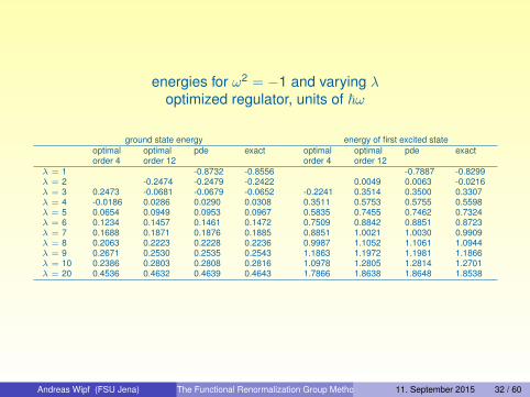
energies for ω2 = −1 and varying λoptimized regulator, units of ~ω

ground state energy energy of first excited stateoptimal optimal pde exact optimal optimal pde exactorder 4 order 12 order 4 order 12

λ = 1 -0.8732 -0.8556 -0.7887 -0.8299λ = 2 -0.2474 -0.2479 -0.2422 0.0049 0.0063 -0.0216λ = 3 0.2473 -0.0681 -0.0679 -0.0652 -0.2241 0.3514 0.3500 0.3307λ = 4 -0.0186 0.0286 0.0290 0.0308 0.3511 0.5753 0.5755 0.5598λ = 5 0.0654 0.0949 0.0953 0.0967 0.5835 0.7455 0.7462 0.7324λ = 6 0.1234 0.1457 0.1461 0.1472 0.7509 0.8842 0.8851 0.8723λ = 7 0.1688 0.1871 0.1876 0.1885 0.8851 1.0021 1.0030 0.9909λ = 8 0.2063 0.2223 0.2228 0.2236 0.9987 1.1052 1.1061 1.0944λ = 9 0.2671 0.2530 0.2535 0.2543 1.1863 1.1972 1.1981 1.1866λ = 10 0.2386 0.2803 0.2808 0.2816 1.0978 1.2805 1.2814 1.2701λ = 20 0.4536 0.4632 0.4639 0.4643 1.7866 1.8638 1.8648 1.8538


Scalar Field TheoryQM = 1-dimensional field theoryNow: Euclidean scalar field theory in d dimensions

L =12

(∂µφ)2 + V (φ)

first: local potential approximation (LPA)

Γk [ϕ] =

∫ddx

(12

(∂µϕ)2 + uk (ϕ)

)second functional derivative: Γ

(2)k = −∆+ u′′k (ϕ)

flow of effective potential: may assume constant average field

∂kuk (q) =12

∫ddp

(2π)d∂kRk (p)

p2 + u′′k (q) + Rk (p)(12)


optimized regulator:⇒ volume of the d-dimensional ball divided by (2π)d ,

µd =1

(4π)d/2Γ(d/2 + 1)

p-integration can be done→ flow equation

∂kuk (ϕ) = µdkd+1

k2 + u′′k (ϕ)(13)

dimensions enters via kd+1 and µd

nonlinear PDEpolynomial ansatz for even potential


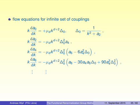
flow equations for infinite set of couplings

kda0

dk= +µdkd+2∆0, ∆0 =

1k2 + a2

,

kda2

dk= −µdkd+2∆2

0a4 ,

kda4

dk= −µdkd+2∆2

0

(a6 − 6a2

4∆0

),

kda6

dk= −µdkd+2∆2

0

(a8 − 30a4a6∆0 + 90a3

4∆20

),

......


Fixed points

K2

K1

line of critical points

T < Tc

T > Tc

(K∗1,K∗

2): fixed point

(K1c,K2c): critical point


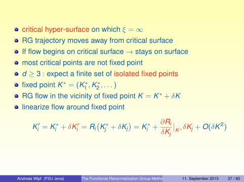
critical hyper-surface on which ξ =∞RG trajectory moves away from critical surfaceIf flow begins on critical surface→ stays on surfacemost critical points are not fixed pointd ≥ 3 : expect a finite set of isolated fixed pointsfixed point K ∗ = (K ∗1 ,K

∗2 , . . . )

RG flow in the vicinity of fixed point K = K ∗ + δKlinearize flow around fixed point

K ′i = K ∗i + δK ′i = Ri(K ∗j + δKj

)= K ∗i +

∂Ri

δKj

∣∣K∗δKj + O(δK 2)


linearized RG transformation,

δK ′i =∑

j

M ji δKj , M j

i =∂Ri

∂Kj

∣∣∣K∗

eigenvalues and left-eigenvectors Φα of matrix M∑j

ΦjαM i

j = λαΦiα = byαΦi

α

every λα defines a critical exponent yαconsider the new variables

gα =∑

i

ΦiαδKi .


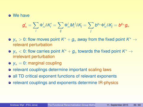
We have

g′α =∑

i

ΦiαδK

′i =

∑ij

ΦiαM j

i δKj =∑

j

byαΦjαδKj = byαgα

yα > 0: flow moves point K ∗ + gα away from the fixed point K ∗ →relevant perturbationyα < 0: flow carries point K ∗ + gα towards the fixed point K ∗ →irrelevant perturbationyα = 0: marginal couplingrelevant couplings determine important scaling lawsall TD critical exponent functions of relevant exponentsrelevant couplings and exponents determine IR-physics


Fixed point analysis for scalar models

introduce the dimensionless field and potential,

ϕ = k (d−2)/2√µd χ and uk (ϕ) = kdµdvk (χ)

flow equation in terms of dimensionless quantities

k∂kvk + dvk −d − 2

2χv ′k =

11 + v ′′k

, v ′k =∂vk

∂χ. . .

at a fixed point: ∂kvk = 0⇒fixed point equation for effective potential

dv∗ −d − 2

2χv ′∗ =

11 + v ′′∗


constant solution dv∗ = 1→ trivial Gaussian fixed pointare there non-Gaussian fixed points?answer depends on the dimension d of spacetimeeven classical potential→ vk even as well:

vk (χ) = wk (%), with % =χ2

2

flow equation for wk (%)

k∂kwk (%) + dwk (%)− (d − 2) %w ′k (%) =1

1 + w ′k (%) + 2%w ′′k (%)

fixed point equation

dw∗(%)− (d − 2) %w ′∗(%) =1

1 + w ′∗(%) + 2%w ′′∗ (%)


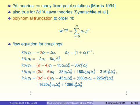
2d theories:∞ many fixed-point solutions [Morris 1994]also true for 2d Yukawa theories [Synatschke et al.]polynomial truncation to order m:

w (m) =m∑

n=0

cn %n

flow equation for couplings

k∂k c0 = −dc0 + ∆0, ∆0 = (1 + c1)−1 ,

k∂k c1 = −2c1 − 6c2∆20 ,

k∂k c2 = (d − 4)c2 − 15c3∆20 + 36c2

2∆30

k∂k c3 = (2d − 6)c3 − 28c4∆20 + 180c2c3∆3

0 − 216c32∆4

0 ,

k∂k c4 = (3d − 8)c4 − 45c5∆20 + (336c2c4 + 225c2

3)∆30

− 1620c22c3∆4

0 + 1296c42∆5

0

......


Scalar fields in three dimensions

expect nontrivial fixed point in d = 3first: polynomial truncation⇒ set ck = 0 for k > minsert into above system of equations with lhs = 0⇒ m algebraic equations for the m + 1 fixed-point couplings

0 = f0(c∗0, c∗1) = f1(c∗1, c

∗2) = · · · = fm−1(c∗1, . . . , c

∗m)

polynomials in c∗0, c∗2, . . . , c

∗m and ∆0 = 1/(1 + c∗1)

prescribe c∗1 (= slope at origin) and thus ∆0

solve the system for c∗0, c∗2, c∗3, . . . , c

∗m in terms of c∗1

algebraic computer program→ solution for m up to 42


explicit expression for the lowest fixed-point couplings

c∗0 =13

11 + c∗1

c∗2 = −c∗1(1 + c∗1)2

3

c∗3 =c∗1(1 + c∗1)3(1 + 13c∗1)

45

c∗4 = −c∗21 (1 + c∗1)4(1 + 7c∗1)

21,

......

c∗m = c∗21 (1 + c∗1)mPm−3(c∗1) ,

Pk polynomial of order k


trivial solution (Gaussian fixed point w ′∗ = 1)

c∗0 =13, 0 = c∗2 = c∗3 = c∗4 = . . .

search for other fixed points:set c∗m = 0→ Pm−3(c∗1) = 0polynomials Pk has many real roots c∗1for each m choose c∗1 such that convergence for large mthe approximating polynomials converge to a power series withmaximal radius of convergenceexample:m = 20⇒ c∗1 = −.186066m = 42⇒ c∗1 = −.186041calculate other c∗k ⇒ fixed point solution


With n! multiplied fixed-point coefficients c∗n

c∗0 c∗1 c∗2 c∗3 c∗4 c∗5 c∗6m = 20 0.409534 -0.186066 0.082178 0.018981 0.005253 0.001104 -0.000255m = 42 0.409533 -0.186064 0.082177 0.018980 0.005252 0.001104 -0.000256

c∗7 c∗8 c∗9 c∗10 c∗11 c∗12 c∗13m = 20 -0.000526 -0.000263 0.000237 0.000632 0.000438 -0.000779 -0.002583m = 42 -0.000526 -0.000263 0.000236 0.000629 0.000431 -0.000799 -0.002643

c∗14 c∗15 c∗16 c∗17 c∗18 c∗19 c∗20m = 20 -0.002029 0.007305 0.028778 0.034696 -0.077525 -0.381385 0.000000m = 42 -0.002216 0.006677 0.026544 0.026320 -0.110498 -0.517445 -0.587152

c∗k stable when one increases polynomial order m (m & 2k )


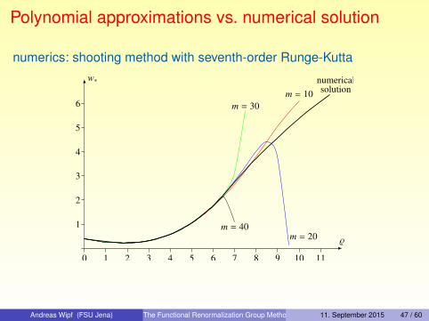
Polynomial approximations vs. numerical solution

numerics: shooting method with seventh-order Runge-Kuttaw∗

0 1 2 3 4 5 6 7 8 9 10 11

1

2

3

4

5

6

m = 10

m = 20

m = 30

m = 40

numerical

solution


fine-tune slope at origin → w ′∗(0) ≈ −0.186064249376Polynomial of degree 42→ w ′∗(0) ≈ −0.186064279993

Critical exponents

flow equation in the vicinity of fixed-point solution w∗set wk = w∗ + δk , linearize the flow in small δk

→ linear differential equation for the small fluctuations

k∂kδk =− dδk + (d − 2) %δ′k

−(dw∗ − (d − 2) %w ′∗

)2 (δ′k + 2%δ′′k

)insert the polynomial approximation for fixed-point solutionpolynomial ansatz for the perturbation→

δk (%) =m−1∑n=0

dn%n % =

χ2

2


linear system for the coefficients dm

k∂k

d0d1...

dm−1

= M (c∗)

d0d1...

dm−1

critical exponents = eigenvalues of m-dimensional matrix M→ up to order m = 46 with algebraic computer program


m ν = −1/ω1 ω2 ω3 ω4 ω5

10 0.648617 0.658053 2.985880 7.502130 17.91349414 0.649655 0.652391 3.232549 5.733445 9.32485818 0.649572 0.656475 3.186784 5.853987 9.14109322 0.649554 0.655804 3.170538 5.977066 8.52281126 0.649564 0.655629 3.182910 5.897290 8.84463230 0.649562 0.655791 3.180847 5.903039 8.90760734 0.649561 0.655749 3.178636 5.922910 8.70258338 0.649562 0.655731 3.180577 5.908885 8.81422542 0.649562 0.655755 3.180216 5.909910 8.84738646 0.649562 0.655746 3.179541 5.915754 8.738608

convergencetwo negative exponents ω0 = −3 and ω1 = −1/νω0 ground state energy, unrelated to critical behaviorω2, ω3, ω4, . . . all positive (irrelevant)LPA-prediction: ν = 0.649562 (high-T expansion: ν = 0.630)


Wave function renormalization

next-to-leading in derivative expansion→wave function renormalization Zk (p, ϕ)

difficult non-linear parabolic partial differential RG-equationsfirst step: neglect field and momentum dependence→

Γk [ϕ] =

∫ddx

(12

Zk (∂µϕ)2 + uk (ϕ)

).

second functional derivative Γ(2)k = −Zk∆+ u′′k (ϕ)

flow equation (simplification for Rk → ZkRk ):∫ddx

(12

(∂kZk ) (∂µϕ)2 + ∂kuk (ϕ)

)=

12

tr(

∂k (ZkRk )

Zk (p2 + Rk ) + u′′k (ϕ)

)


simple: flow of effective potential:

∂kuk =Zk

Zkk2 + u′′k, Zk =

µd

d + 2∂k

(kd+2Zk

).

more difficult: flow of Zk

project flow on operator (∂φ)2

must admit non-homogeneous fields→ [p2,u′′k (ϕ)] 6= 0final answer

k∂kZk = −µd kd+2(

Zka3∆20

)2, ∆0 =

1Zkk2 + a2

see A. Wipf, Lecture Notes in Physics 864

anomalous dimension

η = −k∂k log Zt


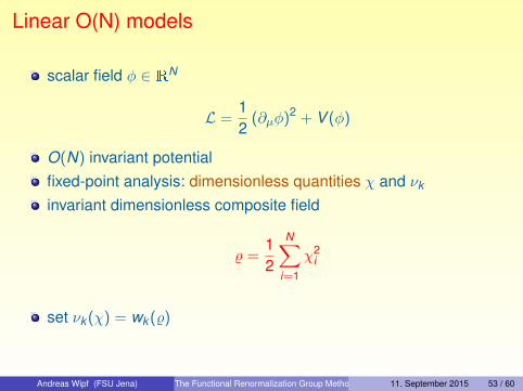
Linear O(N) models

scalar field φ ∈ RN

L =12

(∂µφ)2 + V (φ)

O(N) invariant potentialfixed-point analysis: dimensionless quantities χ and νk

invariant dimensionless composite field

% =12

N∑i=1

χ2i

set νk (χ) = wk (%)


flow equation in LPA (optimized regulator)

k∂kwk + dwk − (d − 2) %w ′k =N − 11 + w ′k

+1

1 + w ′k + 2%w ′′k

contribution of the N − 1 Goldstone modescontribution of massive radial modelarge N: Goldstone modes give dominant contributionlinearize about fixed-point solution: wk = w∗ + δk

fluctuation δk obeys the linear differential equation

k∂kδk = −dδk + (d − 2) %δ′k −(N − 1) δ′k(1 + w ′∗)2 −

δ′k + 2%δ′′k(1 + w ′∗ + 2%w ′′∗ )2


proceed as before: polynomial truncation to high order (40)→ slope at origin of fixed-point solutionfind always Wilson-Fisher fixed pointeigenvalue ω0 = −3 of the scaling operator 1 not listed

N 1 2 3 100 1000−w ′∗(0) 0.186064 0.230186 0.263517 0.384172 0.387935ν = −1/ω1 0.64956 0.70821 0.76113 0.99187 0.99923ω2 0.6556 0.6713 0.6990 0.97218 0.99844ω3 3.1798 3.0710 3.0039 2.98292 2.99554

extract asymptotic formulas

w ′∗(0) ≈ −0.3881 +0.4096

N, ν ≈ 0.9998− 0.9616

N

νexact ≈ 1− 1.081N


Large N Limit

rather simple flow equation (t = log(k/Λ)⇒ ∂t = k∂k , wk ≡ w)

∂tw = (d − 2) %w ′ − dw +N

1 + w ′

⇒ ∂tw ′ = (d − 2) %w ′′ − 2w ′ − N(1 + w ′)2 w ′′

can be solved exactly with methods of characteristicsanalytic relation between fixed point solution and perturbation in

s(t , ρ) ≈ w∗(ρ) + eωtδ(ρ)

result:δ(ρ) = const w ′∗(%)(ω+d)/2 .


if perturbation regular→ all critical exponents

ω ∈ {2n − d |n = 0,1,2, . . . }

one-parameter family of fixed point solutions

/N

w′∗

N = 103

0 1−1

−3π/44−4

−1

1

2


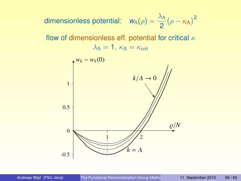
dimensionless potential: wΛ(ρ) =λΛ

2(ρ− κΛ

)2

flow of dimensionless eff. potential for critical κλΛ = 1, κΛ = κcrit

/N

wk − wk(0)

1 2

-0.5

0

0.5

1

k = Λ

k/Λ→ 0


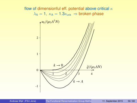
flow of dimensionful eff. potential above critical κλΛ = 1, κΛ = 1.3κcrit ⇒ broken phase

˜/(µ3ΛN)

uk/(µ3Λ3N)

1 2 3 4

-1

0

1

2

k → Λ

k → 0


flow of dimensionful eff. potential below critical κλΛ = 1, κΛ = 0.5κcrit ⇒ symmetric phase

˜/(µ3ΛN)

uk/(µ3Λ3N)

1 1.5 2

0

0.5

1

k → Λ

k → 0


the functional renormalization group method an … · the callan-symanzik regulator: rk(p) = k2...

Documents